EVERSERIES USER’S GUIDE - AASHTOWare Pavement … User Guide_Specific... · Department of...
59
Everseries Users Guide INFORMATION AND CHAPTERS IN SUPPORT OF THE BACKCALCULATION TOOL WERE EXTRACTED FROM: EVERSERIES © USER’S GUIDE Pavement Analysis Computer Software and Case Studies August 2005 Washington State Department of Transportation Environmental and Engineering Programs Materials Laboratory - Pavements Division
-
Upload
nguyenthuy -
Category
Documents
-
view
216 -
download
0
Transcript of EVERSERIES USER’S GUIDE - AASHTOWare Pavement … User Guide_Specific... · Department of...

Everseries Users Guide
INFORMATION AND CHAPTERS IN SUPPORT OF THE BACKCALCULATION TOOL WERE EXTRACTED FROM:
EVERSERIES© USER’S GUIDE Pavement Analysis Computer Software and Case Studies August 2005
Washington State Department of Transportation
Environmental and Engineering Programs Materials Laboratory - Pavements Division

Everseries Users Guide
Forward
This user’s guide includes descriptions of four computer software programs and three case studies, which will highlight hot mix asphalt overlay and design procedures.
The units used in this guide will be US customary. The three WSDOT computer programs – Everstress©, Evercalc©, and Everpave© – are capable of calculating in both US customary and in metric units. The AASHTO computer program AASHTO DARWin®, at the writing of this user’s guide, was only capable of using US customary units.

Everseries Users Guide

Everseries Users Guide
Additional References
Additional references for the Everseries© pavement analysis software programs can be found in the following publications:
1. Bu-Bushait, A., “Development of a Flexible Pavement Fatigue Model for Washington State”, Ph. D. Dissertation, University of Washington, Seattle, Washington, 1985.
2. Newcomb, D. E., “Development and Evaluation of a Regression Method to Interpret Dynamic Pavement Deflections”, Ph. D. Dissertation, University of Washington, Seattle, Washington, 1986.
3. Lee, S. W., “Backcalculation of Pavement Moduli by Use of Pavement Surface Deflections”, Ph. D. Dissertation, University of Washington, Seattle, Washington, 1988.
4. Lee, S. W., Mahoney, J. P., and Jackson, N. C., “A Verification of Backcalculation of Pavement Moduli”, Transportation Research Board No. 1196, Transportation Research Board, Washington DC, 1988.
5. Sivaneswaran, N., Kramer, S. L., and J. P. Mahoney, “Advanced Backcalculation Using a Nonlinear Least Squares Optimization Technique”, Transportation Research Board No. 1293, Transportation Research Board, Washington DC, 1991.
6. Sivaneswaran, N., “Applications of System Identification in Geotechnical Engineering”, Ph. D. Dissertation, University of Washington, Seattle, Washington, 1993.
7. Mahoney, J. P., Winters, B. C., Jackson, N. C., and Pierce, L. M., “Some Observations about Backcalculation and Use of a Stiff Layer Condition”, Transportation Research Board No. 1384, Transportation Research Board, Washington DC, 1993.
8. Pierce, L. M., Jackson, N. C., and Mahoney, J. P., “Development and Implementation of a Mechanistic-Empirical Based Overlay Design Procedure for Flexible Pavements”, Transportation Research Board No. 1388, Transportation Research Board, Washington DC, 1993.
9. Mahoney, J. P. and Pierce, L. M., “An Examination of WSDOT Transfer Functions for Mechanistic-Empirical AC Overlay Design”, Transportation Research Board No. 1539, Transportation Research Board, Washington DC, 1996.
10. Pierce, L. M. and Mahoney, J. P., “Asphalt Concrete Overlay Design Case Studies”, Transportation Research Board No. 1543, Transportation Research Board, Washington DC, 1996.

Everseries Users Guide
Software Disclaimer
The Washington State Department of Transportation does not warrantee anything concerning any of the programs or files, which make up the Everseries© Pavement Analysis Programs. We accept no responsibility for any loss or damage of any kind, which results from the use or purported use of the Everseries© Pavement Analysis Programs, or any files in the package, for any purpose whatsoever.

Everseries Users Guide
Evercalc© — Backcalculation
2.1 FUNDAMENTALS OF BACKCALCULATION
Backcalculation is essentially a mechanistic evaluation, usually an elastic analysis of pavement surface deflection basins generated by various pavement deflection devices. Backcalculation is where measured and calculated surface deflection basins are matched (to within some tolerable error) and the associated layer moduli required to achieve that match are determined. The backcalculation process is usually iterative and normally done with software that can run on microcomputers. General backcalculation guidelines are contained in paragraph 2.5. An illustration of the backcalculation process is shown in Figure 7 and Figure 8.
D 0
D 1 D 2 D 3
P L o a d P l a t e
D e f l e c t i o n B a s i n
A C
B a s e
( S t r e s s Z o n e )
S t i f f ( R i g i d ) L a y e r
Figure 1. Illustration of Backcalculation to Estimate Layer Moduli
2.1.1 Typical Flowchart
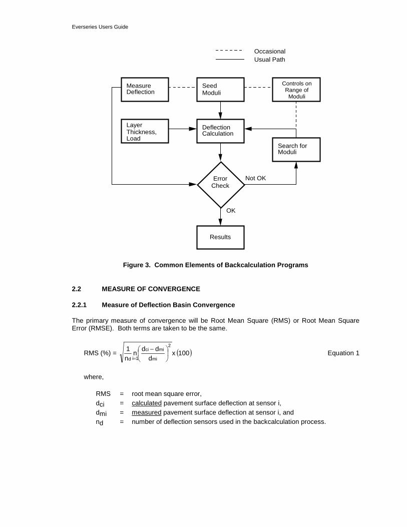
A basic flowchart which represents the fundamental elements in all known backcalculation programs is shown in Figure 9. This flowchart was patterned after one shown by Lytton [2]. Briefly, these elements include:
(a) Measured deflections: Includes the measured pavement surface deflections and associated distances from
the load.
(b) Layer thicknesses and loads: Includes all layer thicknesses and load levels for a specific test location.

Everseries Users Guide
Figure 2. The Backcalculation Process – Matching Measured and Calculated Deflection Basins
(c) Seed moduli: The seed moduli are the initial moduli used in the computer program to calculate
surface deflections. These moduli are usually estimated from user experience or various equations.
(d) Deflection calculation: Layered elastic computer programs such as CHEVRON, BISAR, or ELSYM5 are
generally used to calculate a deflection basin.
(e) Error check: This element simply compares the measured and calculated basins. There are various
error measures, which can be used to make such comparisons.
(f) Search for new moduli: Various methods have been employed within the various backcalculation programs to
converge on a set of layer moduli, which produces an acceptable error between the measured and calculated deflection basins.
(g) Controls on the range of moduli: In some of the backcalculation programs, a range (minimum and maximum) of moduli
are selected or calculated to prevent program convergence to unreasonable moduli levels (could be too high or low).
Everseries Users Guide
Measure Deflection
Layer Thickness, Load
Seed Moduli
Deflection Calculation
Controls on Range of
Moduli
Search for Moduli
Error Check
Results
Not OK
OK
Occasional Usual Path
Figure 3. Common Elements of Backcalculation Programs
2.2 MEASURE OF CONVERGENCE
2.2.1 Measure of Deflection Basin Convergence
The primary measure of convergence will be Root Mean Square (RMS) or Root Mean Square Error (RMSE). Both terms are taken to be the same.
RMS (%) = ( )100x d
ddnn1 2
mi
mici
1id
−
= Equation 1
where,
RMS = root mean square error, dci = calculated pavement surface deflection at sensor i, dmi = measured pavement surface deflection at sensor i, and nd = number of deflection sensors used in the backcalculation process.

Everseries Users Guide
Example RMS calculation
Deflections (mils) Nd Measured Calculated
1 (0") 5.07 4.90 2 (8") 4.32 3.94 3 (12") 3.67 3.50 4 (18") 2.99 3.06 5 (24") 2.40 2.62 6 (36") 1.69 1.86 7 (60") 1.01 0.95
RMS (%) = 22
01.101.195.0...
01.107.590.4
71
−
++
−
= 6.9% (which is very high)
Generally an adequate range of RMS is 1 to 2 percent.
2.3 DEPTH OF STIFF LAYER
Recent literature provides at least two approaches for estimating the depth to stiff layer [3, 4]. The approach used by Rohde and Scullion [3] will be summarized below. There are two reasons for this selection: (1) initial verification of the validity of the approach is documented, and (2) the approach is used in MODULUS 4.0 — a backcalculation program widely used in the U.S.
(a) Basic Assumptions and Description
A fundamental assumption is that the measured pavement surface deflection is a result of deformation of the various materials in the applied stress zone; therefore, the measured surface deflection at any distance from the load plate is the direct result of the deflection below a specific depth in the pavement structure (which is determined by the stress zone). This is to say that only that portion of the pavement structure which is stressed contributes to the measured surface deflections. Further, no surface deflection will occur beyond the offset (measured from the load plate) which corresponds to the intercept of the applied stress zone and the stiff layer (the stiff layer modulus being 100 times larger than the subgrade modulus). Thus, the method for estimating the depth to stiff layer assumes that the depth at which zero deflection occurs (presumably due to a stiff layer) is related to the offset at which a zero surface deflection occurs. This is illustrated in Figure 10 where the surface deflection Dc is zero.

Everseries Users Guide
Figure 4. Illustration of Zero Deflection Due to a Stiff Layer
An estimate of the depth at which zero deflection occurs can be obtained from a plot of
measured surface deflections and the inverse of the corresponding offsets 1
r . This is
illustrated in Figure 11. The middle portion of the plot is linear with either end curved due to nonlinearities associated with the upper layers and the subgrade. The zero surface
deflection is estimated by extending the linear portion of the D vs. 1r plot to a D = 0, the 1r
intercept being designated as r0. Due to various pavement section-specific factors, the depth to stiff layer cannot be directly estimated from r0 — additional factors must be considered. To do this, regression equations were developed based on BISAR computer program generated data for the following factors and associated values:
Load = P = 9000 lbs (40 kN) (only load level considered)
Moduli ratios: SG
1
EE
= 10, 30, 100
SG
2
EE
= 0.3, 1.0, 3.0, 10.0
SG
rigid
EE
= 100

Everseries Users Guide
Figure 5. Plot of Inverse of Deflection Offset vs. Measured Deflection
Thickness levels: T1 = 1, 3, 5, and 10 inches (25, 75, 125, 250 mm) T2 = 6, 10, and 15 inches (150, 250, 375 mm) B = 5, 10, 15, 20, 25, 30, and 50 feet
(1.5, 3.0, 4.5, 6.0, 7.5, 9.0, 15.0 m)
where
Ei = elastic modulus of layer i, Ti = thickness of layer i, B = depth of the rigid (stiff) layer measured from the pavement surface (feet).
The resulting regression equations follow in (b).
(b) Regression Equations
Four separate equations were developed for various HMA layer thicknesses. The
dependent variable is 1B and the independent variables are r0 (and powers of r0) and
various deflection basin shape factors such as SCI, BCI, and BDI (see Appendix A).
(i) HMA less than 2 inches (50 mm) thick: 1B = 0.0362 - 0.3242 (r0) + 10.2717 (r02) - 23.6609 (r03) - 0.0037 (BCI) Equation 2
R2 = 0.98
(ii) HMA 2 to 4 inches (50 to 100 mm) thick:

Everseries Users Guide
1B = 0.0065 + 0.1652 (r0) + 5.4290 (r0
2) - 11.0026 (r03) - 0.0004 (BDI) Equation 3
R2 = 0.98
(iii) HMA 4 to 6 inches (100 to 150 mm) thick: 1B = 0.0413 + 0.9929 (r0) - 0.0012 (SCI) + 0.0063 (BDI) - 0.0778 (BCI) Equation 4
R2 = 0.94
(iv) HMA greater than 6 inches (150 mm) thick: 1B = 0.0409 + 0.5669 (r0) + 3.0137 (r0
2) + 0.0033 (BDI) - 0.0665 log (BCI) Equation 5
R2 = 0.97
where
r0 = r1 intercept (extrapolate steepest section of D vs
r1 plot) in units of
ft1
SCI = D0 - D12" (D0 - D305 mm), Surface Curvature Index BDI = D12" - D24" (D305 - D610 mm), Base Damage Index BCI = D24" - D36" (D610 - D914 mm) Base Curvature Index Di = surface deflections (mils) normalized to a 9,000 lb (40 kN) load at an
offset i in feet
(c) Example
Use some typical deflection data to estimate B (depth to stiff layer). The drillers log suggests a stiff layer might be encountered at a depth of 198 inches (5.0 m) (deflection data originally from SHRP).
(i) First, calculate normalized deflections (9,000 lb (40 kN) basis):
Deflections (mils)
Load Level D0 D8 D12 D18 D24 D36 D60
9,512 lb 5.07 4.32 3.67 2.99 2.40 1.69 1.01
(normalized) 9,000 lb 4.76 4.04 3.44 2.80 2.26 1.59 0.95
6,534 lb 3.28 2.69 2.33 1.88 1.56 1.09 0.68

Everseries Users Guide
(ii) Second, estimate r0. Plot Dr vs. r1 (refer to Figure 12):
Dr (mils)
r (inch) r
1 (ft1 )
4.76 0 — 4.04 8 1.50 3.44 12 1.00 2.80 18 0.67 2.26 24 0.50 1.59 36 0.33 0.95 60 0.20
where all Dr normalized to 9,000 lb (40 kN)
(iii) Third, use regression equation in (b)(iv) (for HMA = 7.65 inches (194 mm)) to calculate B:
1B = 0.0409 + 0.5669 (r0) + 3.0137 (r0
2) + 0.0033 (BDI)
- 0.0665 log (BCI)
where
r0 = r1 intercept (refer to Figure 12)
≅ 0 (used steepest part of deflection basin which is for Sensors at 36 and 60 inches)
BDI = D12" - D24" = 3.44 - 2.26 = 1.18 mils
BCI = D24" - D36" = 2.26 - 1.59 = 0.67 mils
1B = 0.0409 + 0.5669 (0) + 3.0137 (02) + 0.0033 (1.18) - 0.0665 log (0.67)
= 0.0564
1B = 1
0.0564 = 17.7 feet (213 inches or 5.4 m)
This value agrees fairly well with "expected" stiff layer conditions at 16.5 feet (5.0 m) as
indicated by the drillers log even though the r1 value equaled zero.
Everseries Users Guide
0
1
2
3
4
5
0 0.2 (60")
1.0 (12")
1.5 (8")
1/r (Inverse of Deflection Offset)
0.33 (36")
0.5 (24")
0.67 (18")
Measured Deflection D (mils)
r
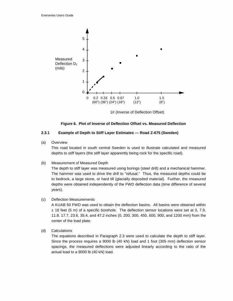
Figure 6. Plot of Inverse of Deflection Offset vs. Measured Deflection
2.3.1 Example of Depth to Stiff Layer Estimates — Road Z-675 (Sweden)
(a) Overview This road located in south central Sweden is used to illustrate calculated and measured depths to stiff layers (the stiff layer apparently being rock for the specific road).
(b) Measurement of Measured Depth The depth to stiff layer was measured using borings (steel drill) and a mechanical hammer. The hammer was used to drive the drill to "refusal." Thus, the measured depths could be to bedrock, a large stone, or hard till (glacially deposited material). Further, the measured depths were obtained independently of the FWD deflection data (time difference of several years).
(c) Deflection Measurements A KUAB 50 FWD was used to obtain the deflection basins. All basins were obtained within ± 16 feet (5 m) of a specific borehole. The deflection sensor locations were set at 0, 7.9, 11.8, 17.7, 23.6, 35.4, and 47.2 inches (0, 200, 300, 450, 600, 900, and 1200 mm) from the center of the load plate.
(d) Calculations The equations described in Paragraph 2.3 were used to calculate the depth to stiff layer. Since the process requires a 9000 lb (40 kN) load and 1 foot (305 mm) deflection sensor spacings, the measured deflections were adjusted linearly according to the ratio of the actual load to a 9000 lb (40 kN) load.
Everseries Users Guide
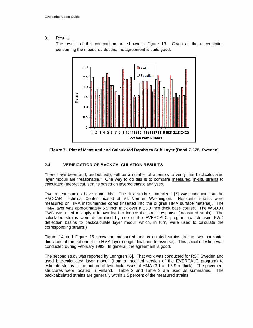
(e) Results The results of this comparison are shown in Figure 13. Given all the uncertainties concerning the measured depths, the agreement is quite good.
Figure 7. Plot of Measured and Calculated Depths to Stiff Layer (Road Z-675, Sweden)
2.4 VERIFICATION OF BACKCALCULATION RESULTS
There have been and, undoubtedly, will be a number of attempts to verify that backcalculated layer moduli are "reasonable." One way to do this is to compare measured, in-situ strains to calculated (theoretical) strains based on layered elastic analyses.
Two recent studies have done this. The first study summarized [5] was conducted at the PACCAR Technical Center located at Mt. Vernon, Washington. Horizontal strains were measured on HMA instrumented cores (inserted into the original HMA surface material). The HMA layer was approximately 5.5 inch thick over a 13.0 inch thick base course. The WSDOT FWD was used to apply a known load to induce the strain response (measured strain). The calculated strains were determined by use of the EVERCALC program (which used FWD deflection basins to backcalculate layer moduli which, in turn, were used to calculate the corresponding strains.)
Figure 14 and Figure 15 show the measured and calculated strains in the two horizontal directions at the bottom of the HMA layer (longitudinal and transverse). This specific testing was conducted during February 1993. In general, the agreement is good.
The second study was reported by Lenngren [6]. That work was conducted for RST Sweden and used backcalculated layer moduli (from a modified version of the EVERCALC program) to estimate strains at the bottom of two thicknesses of HMA (3.1 and 5.9 n. thick). The pavement structures were located in Finland. Table 2 and Table 3 are used as summaries. The backcalculated strains are generally within ± 5 percent of the measured strains.

Everseries Users Guide
Measured Microstrains
Cal
cula
ted
Mic
rost
rain
s
0
50
100
150
200
250
0 50 100 150 200 250
Figure 8. Measured vs. Calculated Strain for Axial Core Bottom Longitudinal Gauges – February 1993 FWD Testing [6]
Measured Microstrains
Cal
cula
ted
Mic
rost
rain
s
0
50
100
150
200
250
300
0 50 100 150 200 250 300
Figure 9. Measured vs. Calculated Strain for Axial Core Bottom Transverse Gauges – February 1993 FWD Testing [6]

Everseries Users Guide
Table 1. Backcalculated and Measured Tensile Strains — 3.1 inch HMA Section [6]
Tensile Strain Bottom of HMA (x 10-6) Time of Day
(a.m. or p.m.) Backcalculated* Measured % Difference
a.m. 119 123 -3 a.m. 119 122 -2 a.m. 74 65 +14 a.m. 60 65 -8 p.m. 284 292 -3 p.m. 284 283 ~0 p.m. 167 159 +5 p.m. 167 158 +6 p.m. 87 85 +2 p.m. 81 84 -4
*Backcalculation process used sensors @ D0, D12, D24, D36, and D48
Table 2. Backcalculated and Measured Tensile Strains — 5.9 inch Section [6]
Tensile Strain Bottom of HMA (x 10-6) Time of Day
(a.m. or p.m.) Backcalculated* Measured % Difference
a.m. 66 70 -6 a.m. 71 69 +3 a.m. 68 69 -1 a.m. 38 35 +9 a.m. 127 130 -2 a.m. 119 130 -8 p.m. 178 185 -4 p.m. 182 183 -1 p.m. 104 96 +8 p.m. 51 48 +6 p.m. 56 49 +14
*Backcalculation process used sensors @ D0, D12, D24, D36, and D48
2.5 BACKCALCULATION GUIDELINES
The general guidelines, which follow, are rather broad in scope and should be considered only “rules-of-thumb” at best. These guidelines were developed from WSDOT experience and the SHRP LTPP Expert Task Group for Deflection Testing and Backcalculation. Undoubtedly, they will change and software such as Evercalc© will continue to be improved.
2.5.1 Number of Layers
Generally, one should use no more than 3 or 4 layers of unknown moduli in the backcalculation process (preferably, no more than 3 layers).
If a three-layer system is being evaluated, and questionable results are being produced (extremely weak base moduli, for example), it is sometimes advantageous to evaluate this pavement structure as a two-layer system. This modification would possibly indicate that the

Everseries Users Guide
base material has been contaminated by the underlying subgrade and is weaker due to the presence of fine material. Alternatively, a stiff layer should be considered if not done so previously.
If a pavement structure consists of a stiffer layer between two weak layers, it may be difficult to obtain realistic backcalculated moduli, such as HMA over a cement treated base.
2.5.1 Thickness of Layers
2.5.1.2 Surfacing
It can be rather difficult to “accurately” backcalculate HMA/BST moduli for bituminous surface layers less than 3 inches (75 mm) thick. Such backcalculation can be attempted for layers less than 3 inches (75 mm), but caution is suggested. In theory, it is possible to backcalculate separate layer moduli for various types of bituminous layers within a flexible pavement. Generally, it is not advisable to do this since one can quickly be attempting to backcalculate too many unknown layer moduli (i.e., greater than 3 or 4). By necessity, one should expect to combine all bituminous layers (seal coats, HMA, etc.) into “one” layer unless there is evidence (or the potential) for distress, such as stripping, in an HMA layer or some other such distress, which is critical to pavement performance.
2.5.1.3 Unstabilized Base/Subbase Course
“Thin” base course beneath “thick” surfacing layers (say HMA or PCC) often result in low base moduli. There are a number of reasons why this can occur. One, a thin base is not a “significant” layer under a very stiff, thick layer. Second, the base modulus may be relatively “low” due to the stress sensitivity of granular materials. The use of a stiff layer generally improves the modulus estimate for base/subbase layers.
2.5.1.4 Subgrade
If unusually high subgrade moduli are calculated, check to see if a stiff layer is present. Stiff layers, if unaccounted for in the backcalculation process, will generally result in unrealistically high subgrade moduli. This is particularly true if a stiff layer is within a depth of about 20 to 30 feet (6 to 9 m) below the pavement surface.
2.5.1.5 Stiff Layer
Often, stiff layers are given “fixed” stiffness ranging from 100,000 to 1,000,000 psi (700 to 7000 MPa) with semi-infinite depth. This, in effect, makes the “subgrade” a layer with a “fixed” depth (instead of the normally assumed infinite depth). Currently, it appears advisable to use backcalculation software, which uses an algorithm such as described and illustrated in Paragraph 2.3, “Depth to Stiff Layer.” What is not so clear is whether one should always fix the depth to stiff layer at say 20, 30, or possibly 50 feet (6, 9, or 15 m) if no stiff layer is otherwise indicated (i.e., use a semi-infinite depth for the subgrade). The depth to stiff layer should be verified whenever possible with other non-destructive testing (NDT) data or borings.
The stiffness (modulus) of the stiff layer apparently can vary. If the stiff layer is due to saturated conditions (e.g. water table) then moduli of about 50,000 psi (345 MPa) appear more appropriate. If rock or stiff glacial tills are the source of the stiff layer then moduli of about 1,000,000 psi (6 900 MPa) appear to be more appropriate.
Everseries Users Guide
2.5.2 Initial Moduli and Moduli Ranges
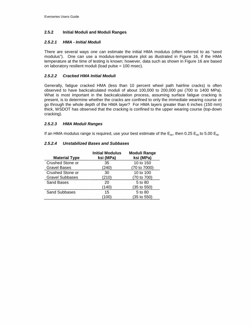
2.5.2.1 HMA - Initial Moduli
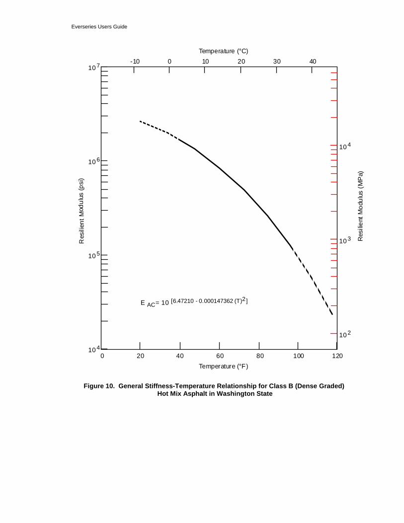
There are several ways one can estimate the initial HMA modulus (often referred to as “seed modulus”). One can use a modulus-temperature plot as illustrated in Figure 16, if the HMA temperature at the time of testing is known; however, data such as shown in Figure 16 are based on laboratory resilient moduli (load pulse = 100 msec).
2.5.2.2 Cracked HMA Initial Moduli
Generally, fatigue cracked HMA (less than 10 percent wheel path hairline cracks) is often observed to have backcalculated moduli of about 100,000 to 200,000 psi (700 to 1400 MPa). What is most important in the backcalculation process, assuming surface fatigue cracking is present, is to determine whether the cracks are confined to only the immediate wearing course or go through the whole depth of the HMA layer? For HMA layers greater than 6 inches (150 mm) thick, WSDOT has observed that the cracking is confined to the upper wearing course (top-down cracking).
2.5.2.3 HMA Moduli Ranges
If an HMA modulus range is required, use your best estimate of the Eac, then 0.25 Eac to 5.00 Eac
2.5.2.4 Unstabilized Bases and Subbases
Initial Modulus Moduli Range Material Type ksi (MPa) ksi (MPa)
Crushed Stone or Gravel Bases
35 (240)
10 to 150 (70 to 7000)
Crushed Stone or Gravel Subbases
30 (210)
10 to 100 (70 to 700)
Sand Bases
20 (140)
5 to 80 (35 to 550)
Sand Subbases
15 (100)
5 to 80 (35 to 550)
Everseries Users Guide
0 20 40 60 80 100 12010 4
10 5
10 6
10 7
Res
ilien
t Mod
ulus
(psi
)
E = 10 [6.47210 - 0.000147362 (T)2]
Temperature (°F)
AC
Res
ilien
t Mod
ulus
(M
Pa)
-10 0 10 20 30 40Temperature (°C)
10 2
10 3
10 4
Figure 10. General Stiffness-Temperature Relationship for Class B (Dense Graded) Hot Mix Asphalt in Washington State

Everseries Users Guide
2.5.2.5 Stabilized Bases and Subbases
If unconfined compressive strength data is available:
Material Type
Unconfined Compressive Strength Initial Modulus Moduli Range
ksi (MPa) ksi (MPa) ksi (MPa) < 250
(< 1.7) 30
(200) 5 to 100
(35 to 690) Lime
Stabilized 250 to 500 (1.7 to 3.4)
50 (340)
15 to 150 (100 to 1000)
> 500 (> 3.4)
70 (480)
20 to 200 (140 to 1400)
< 750 (< 5.2)
400 (2800)
100 to 1500 (700 to 10000)
Cement Stabilized
750 to 1250 (5.2 to 8.6)
1000 (7000)
200 to 3000 (1400 to 20000)
> 1250 (> 8.6)
1500 (10000)
300 to 4000 (2000 to 28000)
If not, assume unconfined compressive strength is 250 to 500 psi (1.7 to 3.4 MPa) for lime stabilized and 750 to 1250 psi (5.2 to 8.6 MPa) for cement stabilized and use corresponding moduli values.
2.5.2.6 Subgrade
The resilient modulus of the subgrade can be determined by
• NDT and backcalculation, • laboratory testing, or • other sources/correlations.
WSDOT will normally use the FWD and appropriate equations to estimate MR. The basic equation for subgrade modulus is [7]:
MR = P (1 - µ2)(p) (r) (dr) (Equation 6)
If µ = 0.5, then the equation reduces to
MR = 0.24 (P)(r) (dr) (Equation 7)
where
MR = elastic modulus of subgrade (psi), P = load (lbs), r = radial distance from the center of the load plate (inch) and dr = pavement deflection at distance r from the applied load (inch).
Refer to Table 4 for suggested typical values or the following discussion and equations to use in estimating Esg (or MR) from the deflection basin.
Everseries Users Guide
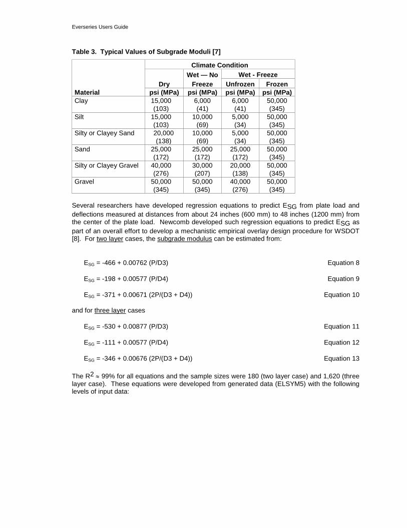
Table 3. Typical Values of Subgrade Moduli [7]
Climate Condition
Dry Wet — No
Freeze Wet - Freeze
Unfrozen Frozen Material psi (MPa) psi (MPa) psi (MPa) psi (MPa) Clay 15,000
(103) 6,000 (41)
6,000 (41)
50,000 (345)
Silt 15,000 (103)
10,000 (69)
5,000 (34)
50,000 (345)
Silty or Clayey Sand 20,000 (138)
10,000 (69)
5,000 (34)
50,000 (345)
Sand 25,000 (172)
25,000 (172)
25,000 (172)
50,000 (345)
Silty or Clayey Gravel 40,000 (276)
30,000 (207)
20,000 (138)
50,000 (345)
Gravel 50,000 (345)
50,000 (345)
40,000 (276)
50,000 (345)
Several researchers have developed regression equations to predict ESG from plate load and deflections measured at distances from about 24 inches (600 mm) to 48 inches (1200 mm) from the center of the plate load. Newcomb developed such regression equations to predict ESG as part of an overall effort to develop a mechanistic empirical overlay design procedure for WSDOT [8]. For two layer cases, the subgrade modulus can be estimated from:
ESG = -466 + 0.00762 (P/D3) Equation 8
ESG = -198 + 0.00577 (P/D4) Equation 9
ESG = -371 + 0.00671 (2P/(D3 + D4)) Equation 10
and for three layer cases
ESG = -530 + 0.00877 (P/D3) Equation 11
ESG = -111 + 0.00577 (P/D4) Equation 12
ESG = -346 + 0.00676 (2P/(D3 + D4)) Equation 13
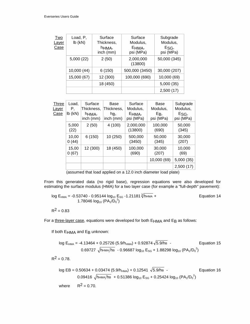
The R2 ≈ 99% for all equations and the sample sizes were 180 (two layer case) and 1,620 (three layer case). These equations were developed from generated data (ELSYM5) with the following levels of input data:
Everseries Users Guide
Two
Layer Case
Load, P, lb (kN)
Surface Thickness,
hHMA, inch (mm)
Surface Modulus, EHMA,
psi (MPa)
Subgrade Modulus,
ESG, psi (MPa)
5,000 (22) 2 (50) 2,000,000 (13800)
50,000 (345)
10,000 (44) 6 (150) 500,000 (3450) 30,000 (207) 15,000 (67) 12 (300) 100,000 (690) 10,000 (69) 18 (450) 5,000 (35) 2,500 (17)
Three Layer Case
Load, P,
lb (kN)
Surface Thickness,
hHMA, inch (mm)
Base Thickness,
hB, inch (mm)
Surface Modulus, EHMA,
psi (MPa)
Base Modulus,
EB, psi (MPa)
Subgrade Modulus,
ESG, psi (MPa)
5,000 (22)
2 (50) 4 (100) 2,000,000 (13800)
100,000 (690)
50,000 (345)
10,000 (44)
6 (150) 10 (250) 500,000 (3450)
50,000 (345)
30,000 (207)
15,000 (67)
12 (300) 18 (450) 100,000 (690)
30,000 (207)
10,000 (69)
10,000 (69) 5,000 (35) 2,500 (17)
(assumed that load applied on a 12.0 inch diameter load plate)
From this generated data (no rigid base), regression equations were also developed for estimating the surface modulus (HMA) for a two layer case (for example a "full-depth" pavement):
log EHMA = -0.53740 - 0.95144 log10 ESG -1.21181 3 HMAh + Equation 14 1.78046 log10 (PA1/D0
2)
R2 = 0.83
For a three-layer case, equations were developed for both EHMA and EB as follows:
If both EHMA and EB unknown:
log EHMA = -4.13464 + 0.25726 (5.9/hHMA) + 0.92874 B5.9/h - Equation 15
0.69727 BHMA hh - 0.96687 log10 ESG + 1.88298 log10 (PA1/D02)
R2 = 0.78.
log EB = 0.50634 + 0.03474 (5.9/hHMA) + 0.12541 B5.9/h - Equation 16
0.09416 BHMA hh + 0.51386 log10 ESG + 0.25424 log10 (PA1/D02)
where R2 = 0.70.

Everseries Users Guide
The following variables were used in the equations shown above:
P = applied load (lbs) on a 11.8 inch plate, hHMA = surface course thickness (inch), hB = base course thickness (inch), EHMA = surface course modulus (psi), EB = base course modulus (psi), ESG = subgrade modulus (psi), D0 = deflection under center of applied load (inch), D0.67 = deflection at 8 inches from center of applied load (inch), D1 = deflection at 1 foot from center of applied load (inch), D2 = deflection at 2 feet from center of applied load (inch), D3 = deflection at 3 feet from center of applied load (inch), D4 = deflection at 4 feet from center of applied load (inch), and A1 = approximate area under deflection basin out to 3 feet = 2 [2 (D0 + D0.67) + (D0.67 + D1) + 3(D1 + D2) + 3(D2 + D3)] = 4D0 + 6D0.67 + 8D1 + 12D2 + 6D3
2.5.2.7 Assumed Poisson’s Ratio
Material Type Poisson’s Ratio Hot mix asphalt 0.35 Portland Cement Concrete 0.15 - 0.20 Base or Subbase Stabilized 0.25 - 0.35 Unstabilized 0.35 Subgrade Soils Cohesive (fine grain) 0.45 Cohesion less (coarse grain) 0.35 - 0.40 Stiff Layer 0.35 or less
2.5.2.8 Convergence Errors
Root Mean Square Error (RMS)
One should attempt to obtain matches between the calculated and measured deflection basins, in terms of RMS, of about 1 to 2 percent. Often, this cannot be achieved and suggests that the basic input data be checked (such as layer thicknesses). The Area value (see Appendix A) might help in this regard.
General
“High” convergence errors suggest that there exists some fundamental problem with a specific backcalculation effort. The problem could be with the deflection data, layer types, and thicknesses, or lack of material homogeneity, which could include cracked and uncracked conditions. “High” convergence errors do not necessarily mean that the backcalculated layer moduli are “no good.”
2.6 EVERCALC©
Evercalc© is a pavement analysis computer program that estimates the “elastic” moduli of pavement layers. Evercalc© estimates the elastic modulus for each pavement layer, determines the coefficients of stress sensitivity for unstabilized materials, stresses and strains at various depths, and optionally normalizes HMA modulus to a standard laboratory condition (temperature).
Everseries Users Guide
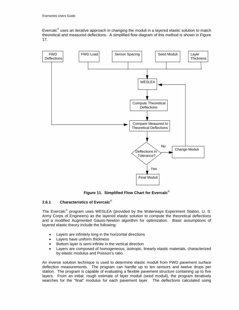
Evercalc© uses an iterative approach in changing the moduli in a layered elastic solution to match theoretical and measured deflections. A simplified flow diagram of this method is shown in Figure 17.
FWD Deflections
FWD Load Sensor Spacing Seed Moduli Layer Thickness
WESLEA
Compute Theoretical Deflections
Compare Measured to Theoretical Deflections
Deflections in Tolerance?
Yes
Final Moduli
No Change Moduli
Figure 11. Simplified Flow Chart for Evercalc©
2.6.1 Characteristics of Evercalc©
The Evercalc© program uses WESLEA (provided by the Waterways Experiment Station, U. S. Army Corps of Engineers) as the layered elastic solution to compute the theoretical deflections and a modified Augmented Gauss-Newton algorithm for optimization. Basic assumptions of layered elastic theory include the following:
• Layers are infinitely long in the horizontal directions • Layers have uniform thickness • Bottom layer is semi infinite in the vertical direction • Layers are composed of homogeneous, isotropic, linearly elastic materials, characterized
by elastic modulus and Poisson’s ratio.
An inverse solution technique is used to determine elastic moduli from FWD pavement surface deflection measurements. The program can handle up to ten sensors and twelve drops per station. The program is capable of evaluating a flexible pavement structure containing up to five layers. From an initial, rough estimate of layer moduli (seed moduli), the program iteratively searches for the “final” modulus for each pavement layer. The deflections calculated using

Everseries Users Guide
WESLEA is compared with the measured ones at each iteration. When the discrepancies in the calculated and measured deflections as characterized by root mean square (RMS) error (Equation 23), or the changes in modulus (Equation 24) falls within the allowable tolerance, or the number of iterations has reached a limit the program terminates. Using the final set of moduli, the stresses and strains at the bottom of the HMA layer, middle of the other layers except the subgrade, and at the top of the subgrade is calculated. When deflection data for more than one load level is available at a given point, coefficients of stress sensitivity for unstabilized materials are also computed. Optionally, HMA layer modulus is normalized to a standard laboratory condition.
2.6.1.1 Seed Moduli
Two options for estimating the seed moduli are available. When a pavement structure containing up to three layers is being analyzed, a set of internal regression equations can be used [8]. These regression equations determine a set of seed moduli from the relationships between the layer modulus, surface deflections, applied load, and layer thickness. Alternatively, the user can provide these values. When more than one deflection data set at a given location is analyzed, the final moduli from the previous deflection data set is used as seed moduli for the next one in order to improve the performance of the program.
2.6.1.2 Termination
The program terminates when one or more of the following conditions are satisfied:
i) Deflection Tolerance:
( )100d
ddn1 (%) RMS
2n
1i mi
mici
d∑
−
==
Equation 17
where, dei and dmi are the measured and calculated deflections at i-th sensor and n- is the number of sensors.
Normally a deflection tolerance of one percent is considered adequate.
ii) Moduli Tolerance:
εm = [E(k+1)i – Eki] x (100) Equation 18 Eki
where, Eki and E(k+1)i are the i-th layer moduli at the k-th and (k+1)-th iteration, respectively, and m- is the number of layers with unknown moduli.
Again, a modulus tolerance of one percent is considered adequate.
iii) Number of iterations has reached the Maximum Number of Iterations. At every iteration a minimum of (m + 1) calls to WESLEA is made, where m- is the number of layers with unknown moduli. Normally, a maximum number of ten iterations is adequate.
2.6.1.3 Coefficients of Stress Sensitivity
The stress sensitivity characteristics of unstabilized material moduli are usually formulated as follows:
Eb = k1θk2 for coarse grained soils Equation 19
Everseries Users Guide
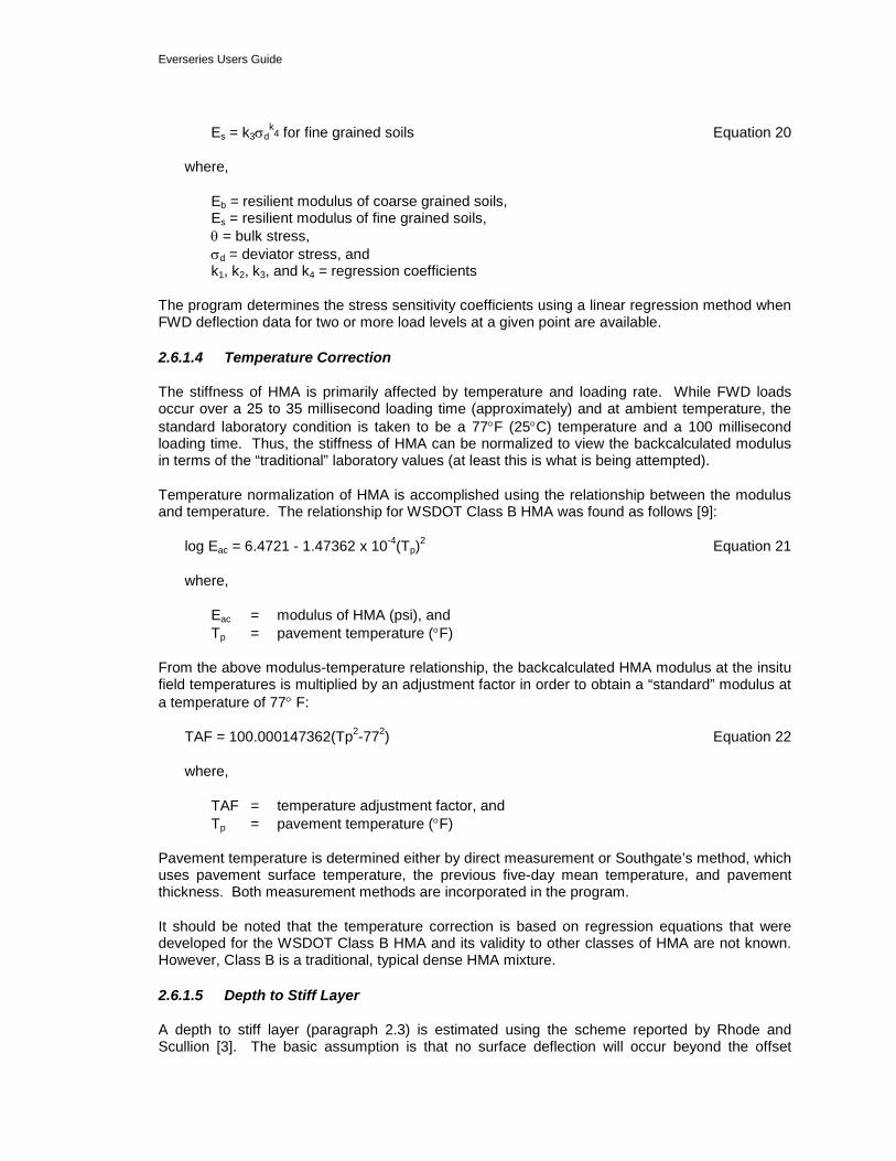
Es = k3σdk4 for fine grained soils Equation 20
where,
Eb = resilient modulus of coarse grained soils, Es = resilient modulus of fine grained soils, θ = bulk stress, σd = deviator stress, and k1, k2, k3, and k4 = regression coefficients
The program determines the stress sensitivity coefficients using a linear regression method when FWD deflection data for two or more load levels at a given point are available.
2.6.1.4 Temperature Correction
The stiffness of HMA is primarily affected by temperature and loading rate. While FWD loads occur over a 25 to 35 millisecond loading time (approximately) and at ambient temperature, the standard laboratory condition is taken to be a 77°F (25°C) temperature and a 100 millisecond loading time. Thus, the stiffness of HMA can be normalized to view the backcalculated modulus in terms of the “traditional” laboratory values (at least this is what is being attempted).
Temperature normalization of HMA is accomplished using the relationship between the modulus and temperature. The relationship for WSDOT Class B HMA was found as follows [9]:
log Eac = 6.4721 - 1.47362 x 10⁻⁴(Tp)2 Equation 21
where,
Eac = modulus of HMA (psi), and Tp = pavement temperature (°F)
From the above modulus-temperature relationship, the backcalculated HMA modulus at the insitu field temperatures is multiplied by an adjustment factor in order to obtain a “standard” modulus at a temperature of 77° F:
TAF = 100.000147362(Tp2-772) Equation 22
where,
TAF = temperature adjustment factor, and Tp = pavement temperature (°F)
Pavement temperature is determined either by direct measurement or Southgate’s method, which uses pavement surface temperature, the previous five-day mean temperature, and pavement thickness. Both measurement methods are incorporated in the program.
It should be noted that the temperature correction is based on regression equations that were developed for the WSDOT Class B HMA and its validity to other classes of HMA are not known. However, Class B is a traditional, typical dense HMA mixture.
2.6.1.5 Depth to Stiff Layer
A depth to stiff layer (paragraph 2.3) is estimated using the scheme reported by Rhode and Scullion [3]. The basic assumption is that no surface deflection will occur beyond the offset
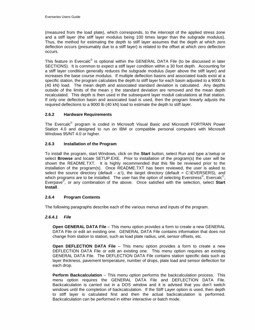
Everseries Users Guide
(measured from the load plate), which corresponds, to the intercept of the applied stress zone and a stiff layer (the stiff layer modulus being 100 times larger than the subgrade modulus). Thus, the method for estimating the depth to stiff layer assumes that the depth at which zero deflection occurs (presumably due to a stiff layer) is related to the offset at which zero deflection occurs.
This feature in Evercalc© is optional within the GENERAL DATA File (to be discussed in later SECTIONS). It is common to expect a stiff layer condition within a 30 foot depth. Accounting for a stiff layer condition generally reduces the subgrade modulus (layer above the stiff layer) and increases the base course modulus. If multiple deflection basins and associated loads exist at a specific station, the program calculates the depth to stiff layer for each basin adjusted to a 9000 lb (40 kN) load. The mean depth and associated standard deviation is calculated. Any depths outside of the limits of the mean + the standard deviation are removed and the mean depth recalculated. This depth is then used in the subsequent layer moduli calculations at that station. If only one deflection basin and associated load is used, then the program linearly adjusts the required deflections to a 9000 lb (40 kN) load to estimate the depth to stiff layer.
2.6.2 Hardware Requirements
The Evercalc© program is coded in Microsoft Visual Basic and Microsoft FORTRAN Power Station 4.0 and designed to run on IBM or compatible personal computers with Microsoft Windows 95/NT 4.0 or higher.
2.6.3 Installation of the Program
To install the program, start Windows, click on the Start button, select Run and type a:\setup or select Browse and locate SETUP.EXE. Prior to installation of the program(s) the user will be shown the README.TXT. It is highly recommended that this file be reviewed prior to the installation of the program(s). Once README.TXT has been reviewed, the user is asked to select the source directory (default - a:\), the target directory (default = C:\EVERSERS), and which programs are to be installed. The user has the option of selecting Everstress©, Evercalc©, Everpave©, or any combination of the above. Once satisfied with the selection, select Start Install.
2.6.4 Program Contents
The following paragraphs describe each of the various menus and inputs of the program.
2.6.4.1 File
Open GENERAL DATA File – This menu option provides a form to create a new GENERAL DATA File or edit an existing one. GENERAL DATA File contains information that does not change from station to station, such as load plate radius, unit, sensor offsets, etc.
Open DEFLECTION DATA File – This menu option provides a form to create a new DEFLECTION DATA File or edit an existing one. This menu option requires an existing GENERAL DATA File. The DEFLECTION DATA File contains station specific data such as layer thickness, pavement temperature, number of drops, plate load and sensor deflection for each drop.
Perform Backcalculation – This menu option performs the backcalculation process. This menu option requires the GENERAL DATA File and DEFLECTION DATA File. Backcalculation is carried out in a DOS window and it is advised that you don’t switch windows until the completion of backcalculation. If the Stiff Layer option is used, then depth to stiff layer is calculated first and then the actual backcalculation is performed. Backcalculation can be performed in either interactive or batch mode.

Everseries Users Guide
Interactive Mode: In interactive mode, the backcalculation is carried out in the foreground and the progress during each iteration and the calculated and measured deflection basins at the end of iteration are displayed on the screen.
Batch Mode: In batch mode, the backcalculation is carried out in the background. The iteration details are saved in a log file having the same name as the DEFLECTION DATA File with the extension .LOG.
If stiff layer option is used the user is presented with a histogram and a table of depth to apparent stiff layer and with the station identifier. The user can choose to accept the calculated depth to stiff layer values or modify it before performing the backcalculation.
Convert FWD DATA File – This menu option converts a raw FWD (Dynatest Model 8000) data file to an Evercalc© DEFLECTION DATA File. This menu option requires an existing GENERAL DATA File. If the deflection data is generated from any other NDT device, other than the Dynatest 8000, this option will not generate the appropriate file format.
Modify Standard Temperature – Since asphalt materials are temperature sensitive and FWD data collection temperature may vary within a specific location and from one location to the next, the establishment of a standard temperature is necessary. WSDOT default standard temperature for the determination of the asphalt moduli to be 77°F (25°C).
Exit – Exit the program and return to the Windows screen.
2.6.4.2 Print
Print/View Output
Displays formatted output data on the screen and provides the option to print on the default printer. The output data contains all calculations for all required iterations and can result in at least 2 pages per station.
Options – standard Windows protocols are used for viewing various pages, zoom, selecting font style for screen view and printing, printing and exiting print screen.
Print/View Summary
Displays formatted summary data on the screen and provides the option to print on the default printer. This data contains the station, layer thickness, moduli for each specified layer, the RMS error.
Options – standard Windows protocols are used for viewing various pages, zoom, selecting font style for screen view and printing, printing and exiting print screen.
Page Setup
Allows the user to modify the page margins. The default settings are shown.

Everseries Users Guide
Select Font
Allows the user to choose any available font for use in displaying and printing the output and summary information. This font is also saved as the default font for future output display.
2.6.4.3 Help
Contents – Contains descriptions of the various program menus and entry requirements for program operation. The help screen is derived from the field descriptions contained in this User’s Guide.
Search for Help on… - Typical Windows format for searching for key program descriptions.
About EVERCALC© - lists program version information, responsible agency and personnel contacts, system memory and resources.
2.6.4.4 Open General File
Title - Any text that describes the GENERAL DATA File
No of Layers - Total number of layers (including the stiff layer, if a stiff layer option is selected). The minimum number of layers is two, and the maximum number of layers is five. Seed moduli will need to be provided if the number of layers is more than three.
No of Sensors - Total number of FWD sensors. Maximum number of sensors is limited to ten.
Units - Units of measurement and output, either Metric or US Customary.
Stiff Layer - Check this option to include a stiff layer. The depth to stiff layer is calculated prior to beginning the backcalculation process. The stiff layer moduli should be provided.
Temp. Correction - Check this option to adjust the moduli of the first layer to the standard temperature.
Temp. Measurement - Required only when temperature correction is required. Select the appropriate temperature measurement option. Choose the Direct Method option if using an HMA mid-depth temperature measurement. Use the Southgate Method option if pavement temperature is to be calculated from surface temperatures and five-day mean air temperatures (requires additional data).
Plate Radius - Radius of the FWD loading plate.
Seed Moduli - Seed moduli are the initial estimates of unknown layer moduli. Choose Internal if you want the program to estimate the seed moduli. The internal option cannot be used when the number of layers is more than three. The user can also specify seed moduli by selecting User Supplied.
Sensor Weigh Factor – This field allows the user to select amongst three options for calculating the error function that drives the backcalculation process. Evercalc© uses uniform as the default method. The three options are described as follows:
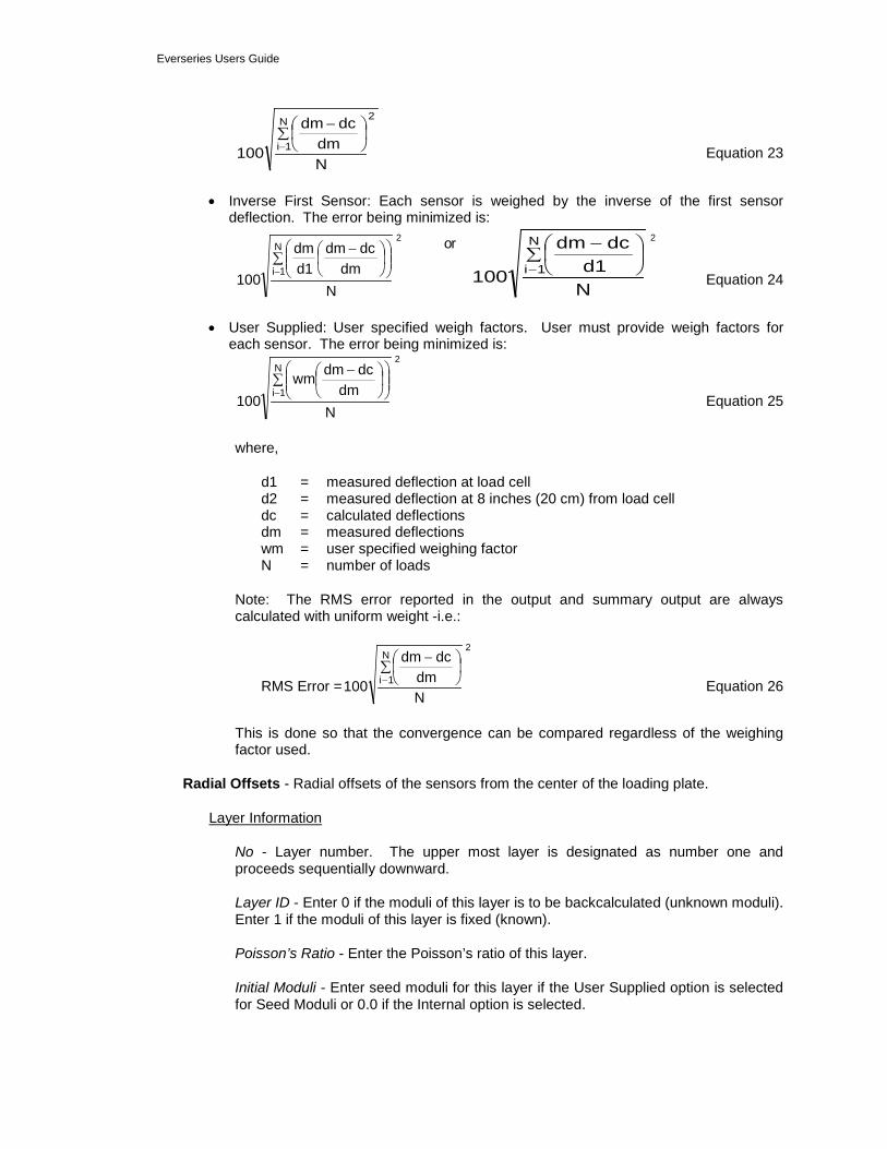
• Uniform: Each sensor deflection is weighed uniformly in constructing the error function. The error being minimized is:
Everseries Users Guide
2N
1i
Ndm
dcdm
100∑
−
− Equation 23
• Inverse First Sensor: Each sensor is weighed by the inverse of the first sensor deflection. The error being minimized is:
Ndm
dcdmd1dm
100
N
1i∑
−
−
2 or
Nd1
dcdm
100
N
1i∑
−
−
2
Equation 24
• User Supplied: User specified weigh factors. User must provide weigh factors for each sensor. The error being minimized is:
Ndm
dcdmwm100
N
1i∑
−
−
2
Equation 25
where,
d1 = measured deflection at load cell d2 = measured deflection at 8 inches (20 cm) from load cell dc = calculated deflections dm = measured deflections wm = user specified weighing factor N = number of loads
Note: The RMS error reported in the output and summary output are always calculated with uniform weight -i.e.:
RMS Error =Ndm
dcdm
100
N
1i∑
−
−
2
Equation 26
This is done so that the convergence can be compared regardless of the weighing factor used.
Radial Offsets - Radial offsets of the sensors from the center of the loading plate.
Layer Information
No - Layer number. The upper most layer is designated as number one and proceeds sequentially downward.
Layer ID - Enter 0 if the moduli of this layer is to be backcalculated (unknown moduli). Enter 1 if the moduli of this layer is fixed (known).
Poisson’s Ratio - Enter the Poisson’s ratio of this layer.
Initial Moduli - Enter seed moduli for this layer if the User Supplied option is selected for Seed Moduli or 0.0 if the Internal option is selected.
Everseries Users Guide
Min. Moduli - Enter the minimum value of the layer moduli for this layer (must be greater than or equal to 0.0). Can be set to 0.0 if no minimum limit is required.
Max. Moduli - Enter the maximum value of the layer moduli for this layer (must be greater than or equal to 0.0). Can be set to 0.0 if no minimum limit is required.
Max. Iteration - Maximum number of iterations allowed during the optimization. A value of ten is typically used.
RMS Tol. (%) - Root mean square error tolerance between the measured and calculated deflections (percentage). A value of 1.0 is typical.
Modulus Tol. (%) - Modulus percentage tolerance in successive iterations. A value of 1.0 is typical.
Stress and Strain Location – allows user to input up to 10 locations for stress and strain computation. The default locations are beneath the center load at the bottom of the asphalt layer, at the middle of the base layer, and at the top of the subgrade.
Save - Saves the current GENERAL DATA File under the same name. The user must save the file after the data is entered. The program will not save automatically or prompt user to save the data file.
Save As - Saves the current GENERAL DATA File under a different name.
Cancel - Discards any changes made without saving and returns the user to the Main Screen.
2.6.4.5 Open DEFLECTION DATA File
Route - Name of the Route or any other descriptive information.
Station Information
Station - Station identification, such as milepost. A maximum character limit of ten.
H(1) to H(4) - Thickness of each pavement layer, up to 5 layers. The last layer thickness is excluded (subgrade or stiff layer are considered to be infinite in depth).
No. of Drops - Total number of drops at this station. A maximum of twelve drops is allowed.
Pavement Temperature - Pavement temperature (if Direct Method) or five-day mean air temperature (if Southgate Method).
Deflection Information
Drop No – The drop number if more than one drop is input. The program allows up to eight drops per station.
Load - Plate load for each drop.
Sensor Deflection - Measured sensor deflection for each drop at each sensor starting from the closest sensor to the farthest sensor.
Everseries Users Guide
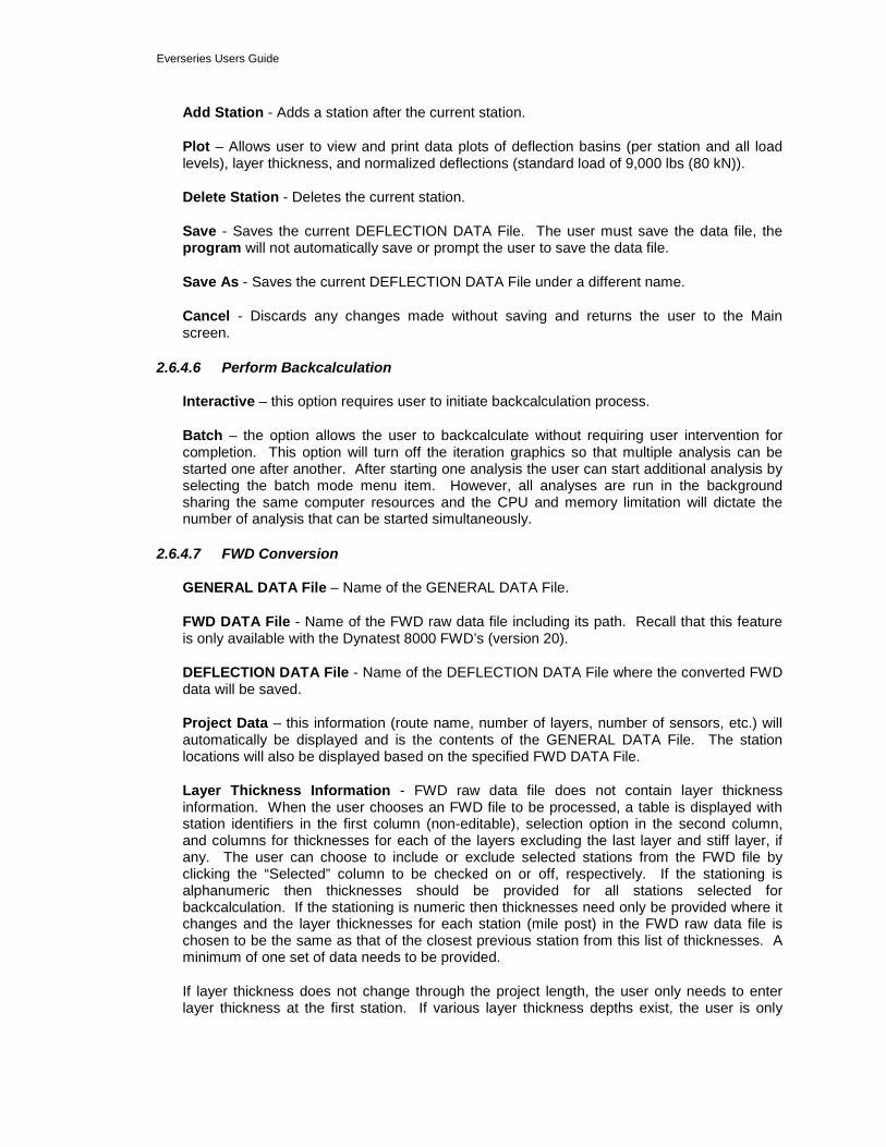
Add Station - Adds a station after the current station.
Plot – Allows user to view and print data plots of deflection basins (per station and all load levels), layer thickness, and normalized deflections (standard load of 9,000 lbs (80 kN)).
Delete Station - Deletes the current station.
Save - Saves the current DEFLECTION DATA File. The user must save the data file, the program will not automatically save or prompt the user to save the data file.
Save As - Saves the current DEFLECTION DATA File under a different name.
Cancel - Discards any changes made without saving and returns the user to the Main screen.
2.6.4.6 Perform Backcalculation
Interactive – this option requires user to initiate backcalculation process.
Batch – the option allows the user to backcalculate without requiring user intervention for completion. This option will turn off the iteration graphics so that multiple analysis can be started one after another. After starting one analysis the user can start additional analysis by selecting the batch mode menu item. However, all analyses are run in the background sharing the same computer resources and the CPU and memory limitation will dictate the number of analysis that can be started simultaneously.
2.6.4.7 FWD Conversion
GENERAL DATA File – Name of the GENERAL DATA File.
FWD DATA File - Name of the FWD raw data file including its path. Recall that this feature is only available with the Dynatest 8000 FWD’s (version 20).
DEFLECTION DATA File - Name of the DEFLECTION DATA File where the converted FWD data will be saved.
Project Data – this information (route name, number of layers, number of sensors, etc.) will automatically be displayed and is the contents of the GENERAL DATA File. The station locations will also be displayed based on the specified FWD DATA File.
Layer Thickness Information - FWD raw data file does not contain layer thickness information. When the user chooses an FWD file to be processed, a table is displayed with station identifiers in the first column (non-editable), selection option in the second column, and columns for thicknesses for each of the layers excluding the last layer and stiff layer, if any. The user can choose to include or exclude selected stations from the FWD file by clicking the “Selected” column to be checked on or off, respectively. If the stationing is alphanumeric then thicknesses should be provided for all stations selected for backcalculation. If the stationing is numeric then thicknesses need only be provided where it changes and the layer thicknesses for each station (mile post) in the FWD raw data file is chosen to be the same as that of the closest previous station from this list of thicknesses. A minimum of one set of data needs to be provided.
If layer thickness does not change through the project length, the user only needs to enter layer thickness at the first station. If various layer thickness depths exist, the user is only

Everseries Users Guide
required to enter thicknesses where changes occur. For example, project limits are from station 0 to station 5, and the following layer thickness exist:
Station
Thickness of Asphalt
H(1)
Thickness of Base
H(2) 0 4.0 inches 6.0 inches
2.5 6.0 inches 8.0 inches
The user would then click on box adjacent to Station 0 and then type in 4.0 for H(1) and 6.0 for H(2). The same process would then be necessary next to station 2.5, click on the box adjacent to Station 2.5 and type in 6.0 for H(1) and 8.0 for H(2). The program will then use 4 inches for the asphalt layer and 6 inches for the base layer from Station 0 to Station 2.5, and 6 inches for the asphalt layer and 8 inches for the base layer from Station 2.5 to Station 5.0.
Select All – Selects all station locations for layer moduli determination.
Deselect All – Deselects all station locations. User selects specific locations for layer moduli determination.
Multiple Drops – Allows user various methods for analyzing data when multiple drops at the same load level are collected.
No – use all the load-deflection data in the backcalculation process. This option is recommended when only one drop per load level has been collected.
Average Normalized – FWD data was collected using multiple drops at each load level. The average load at each load level is determined and then the deflections are averaged and normalized at each load level. For this method the user must enter the number of drops per load. For example, the deflection data is collected using three drops at each load level. This option would then calculate the average load for all three drops (for each load level), then each of the three deflection readings are normalized to the average load and then the normalized deflections are averaged to obtain a single load-deflection data at that load level.
Average – FWD data was collected using multiple drops at each load level. This method averages the load and deflection data. For this method the user must enter the number of drops per load. If the deflection data was collected using multiple drops at each load level, this is the recommended procedure to minimize the random error that is associated with deflection and/or load measurements.
Convert - Converts the FWD raw data file to the necessary format. This process is extremely quick and the user is not prompted that the process is complete.
Exit – Exits the Convert screen and returns to the main screen.
2.6.4.8 Modify Standard Temperature
Allows user to modify the standard temperature for determining the asphalt layer moduli. WSDOT uses 77°F (25°C) as the standard temperature.
2.6.4.9 Exit
Exits the program and returns to Windows.
Everseries Users Guide
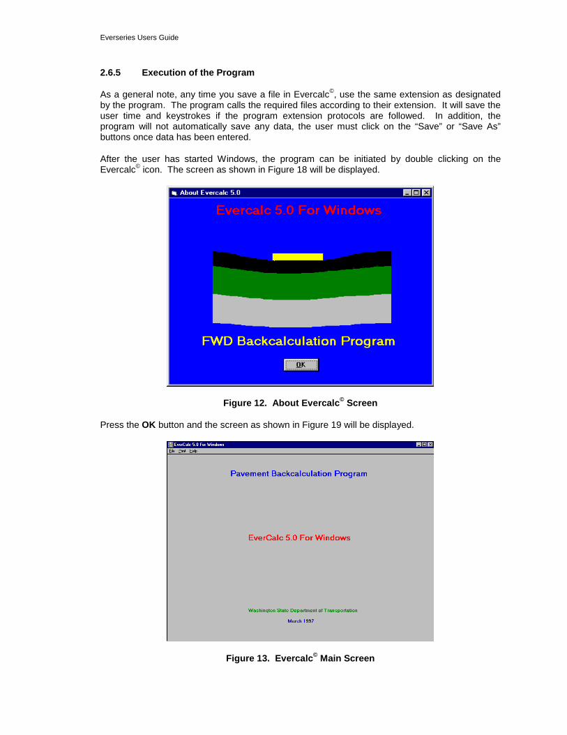
2.6.5 Execution of the Program
As a general note, any time you save a file in Evercalc©, use the same extension as designated by the program. The program calls the required files according to their extension. It will save the user time and keystrokes if the program extension protocols are followed. In addition, the program will not automatically save any data, the user must click on the “Save” or “Save As” buttons once data has been entered.
After the user has started Windows, the program can be initiated by double clicking on the Evercalc© icon. The screen as shown in Figure 18 will be displayed.
Figure 12. About Evercalc© Screen
Press the OK button and the screen as shown in Figure 19 will be displayed.
Figure 13. Evercalc© Main Screen

Everseries Users Guide
The first step for performing the backcalculation process is the development of the GENERAL DATA File. The GENERAL DATA File contains general pavement data and the general specifications of the nondestructive testing device. Select File and then select Open General File to create the GENERAL DATA File. The program will prompt the user for a filename, either select a file that is listed or enter a nonexistent filename to create a new GENERAL DATA File. Once the file has been generated the screen as shown in Figure 20 will be displayed.
Figure 14. General Data Entry Screen
Begin by entering the following data:
* The title of the project * The number of pavement layers. The number of layers is limited to five
layers, including a stiff layer, if used * The number of FWD sensors * The radius of the FWD loading plate * The units of measure * Presence of a stiff layer? * Is temperature correction desired for the HMA layer? Default value for
temperature correction is 77°F (25°C) or can be established by the user by selecting File and Modify Standard Temperature.
* Pavement temperature measured using the Direct or Southgate Method? * Are the seed moduli to be internal or user supplied? If a stiff layer is used, the
user must supply the seed (initial) moduli. * What sensor weigh factor will be used? * The radial offset (inch or cm) of each sensor from the load plate. WSDOT
uses the following sensor spacing: 0, 8 inches (20.3 cm), 12 inches (30.5 cm), 24 inches (61.0 cm), 36 inches (91.5 cm), and 48 inches (122.0 cm). Care must be taken to insure that the most distant sensor from the load is actually measuring a deflection. If this sensor is located too far from the loading plate, the sensor may pick up more “noise” than an actual deflection and may result in higher error than necessary.
* Layer information. Using the scroll bar, input the layer number, layer ID, Poisson’s ratio, initial modulus (ksi or MPa), and if supplied by the user, the minimum and maximum moduli (ksi or MPa) for each of the pavement layers.
* Enter the program termination values: maximum number of iterations, RMS tolerance (in percent) and the modulus tolerance (in percent).
Everseries Users Guide
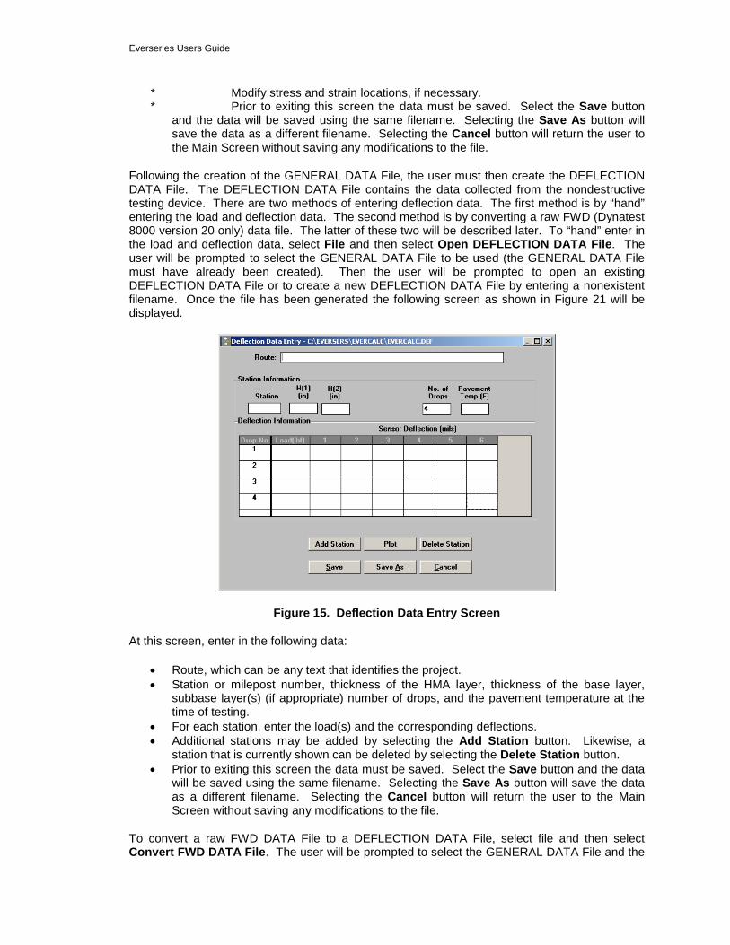
* Modify stress and strain locations, if necessary. * Prior to exiting this screen the data must be saved. Select the Save button
and the data will be saved using the same filename. Selecting the Save As button will save the data as a different filename. Selecting the Cancel button will return the user to the Main Screen without saving any modifications to the file.
Following the creation of the GENERAL DATA File, the user must then create the DEFLECTION DATA File. The DEFLECTION DATA File contains the data collected from the nondestructive testing device. There are two methods of entering deflection data. The first method is by “hand” entering the load and deflection data. The second method is by converting a raw FWD (Dynatest 8000 version 20 only) data file. The latter of these two will be described later. To “hand” enter in the load and deflection data, select File and then select Open DEFLECTION DATA File. The user will be prompted to select the GENERAL DATA File to be used (the GENERAL DATA File must have already been created). Then the user will be prompted to open an existing DEFLECTION DATA File or to create a new DEFLECTION DATA File by entering a nonexistent filename. Once the file has been generated the following screen as shown in Figure 21 will be displayed.
Figure 15. Deflection Data Entry Screen
At this screen, enter in the following data:
• Route, which can be any text that identifies the project. • Station or milepost number, thickness of the HMA layer, thickness of the base layer,
subbase layer(s) (if appropriate) number of drops, and the pavement temperature at the time of testing.
• For each station, enter the load(s) and the corresponding deflections. • Additional stations may be added by selecting the Add Station button. Likewise, a
station that is currently shown can be deleted by selecting the Delete Station button. • Prior to exiting this screen the data must be saved. Select the Save button and the data
will be saved using the same filename. Selecting the Save As button will save the data as a different filename. Selecting the Cancel button will return the user to the Main Screen without saving any modifications to the file.
To convert a raw FWD DATA File to a DEFLECTION DATA File, select file and then select Convert FWD DATA File. The user will be prompted to select the GENERAL DATA File and the

Everseries Users Guide
FWD DATA File to be converted. The screen similar to what is shown in Figure 22 will be displayed.
Figure 16. FWD Data Conversion Screen
The GENERAL DATA File and FWD DATA File that was selected by the user will be shown on the upper portion of this screen. The program will automatically name the DEFLECTION DATA File according to the name used for the FWD DATA File. The program will assign “.DEF” as the DEFLECTION DATA File extension. This screen will convert the raw FWD file into a format to be used in the backcalculation process. In addition, this screen will allow the user to input layer thickness for each of the layers as designated in the GENERAL DATA File. The stations to be included in the deflection data file are selected and the corresponding layer thicknesses are entered as explained earlier. Once all data has been entered, select Convert and the program will execute, and then select Exit to return to the Main screen.
The plot routines that are available in the Deflection Data Entry screen are deflection basin, layer thickness, and normalized deflection. Selecting the Plot button, the following screen will be displayed.
Figure 17. Deflection Data Plot Screen
Each one of these options will be briefly described.

Everseries Users Guide
Deflection Basin – the deflection basin (for all load levels) will be displayed for each individual station location. The buttons across the top of the screen will allow the user various options for presenting the data.
Figure 18. Plot Deflection Basin
Layer Thickness –the various layer thicknesses for the entire deflection data file will be displayed.
Figure 19. Plot Layer Thickness
Normalized Deflection – the normalized (to the standard temperature and 9000 lb (40 kN)) deflection will be displayed according to each sensor for the entire deflection data file.

Everseries Users Guide
Figure 20. Plot Normalized Deflections
After creating the GENERAL DATA File and the DEFLECTION DATA File, the user is now able to begin the backcalculation process. Select File and then select Perform Backcalculation. The user will then have the choice to either run the backcalculation in the interactive or batch mode. If numerous deflection files are to be analyzed and the user does not want to be prompted to complete the analysis (run process over night for example) then the batch mode should be selected. In the interactive mode, the user will be prompted to select the GENERAL DATA File, the DEFLECTION DATA File, and to confirm the Output Filename. If the user selected to not use a stiff layer (GENERAL DATA File), the backcalculation process will begin. If the user selected a stiff layer, then the depth to stiff layer screen will be displayed and the user will be asked to modify the estimated depth to stiff layer or to accept the data as shown (see Figure 27).
Figure 21. Depth to Apparent Stiff Layer Screen

Everseries Users Guide
If the user has actual borings to depth of stiff layer (or saturated layer) they can be entered directly onto this screen. Clicking on the depth to be modified will allow the user to enter the necessary values.
Click on the OK button and the backcalculation process will begin. The program will then display on the screen the measured and calculated deflections in the determination of the layer moduli. The computer will display this screen for each load level at each station. The process is completed when the word “Finished” is displayed in the lower left-hand corner as shown in Figure 28.
Figure 22. Backcalculation Screen
To return back to the main menu, select File and then Exit or close the screen using the X button in the upper right hand corner. The data can then be viewed or printed by selecting Print on the main menu tool bar. To exit the Evercalc© program, select File and then select Exit.
2.6.6 EVERCALC Deflection File Format
2.6.6.1 Sample of Evercalc© Deflection File
SR 14 6TH AVE. TO EVERGREEN BLVD. - Tested on 12/06/95 (description) 18.05 4 4.200 10.320 0.000 0.000 37.000 0.000 (test location 1/description) 17141.0 8.910 8.320 7.760 6.040 4.600 3.460 (load 1/deflection) 12946.0 7.150 6.720 6.220 4.830 3.650 2.720 (load 2/deflection) 9582.0 5.590 5.160 4.800 3.730 2.690 2.110 (load 3/deflection) 6201.0 3.590 3.390 3.100 2.420 1.800 1.290 (load 4/deflection) 16.6 4 5.000 10.560 0.000 0.000 37.000 0.000 (test location 2/description) 16240.0 8.280 7.400 6.970 5.320 3.800 2.690 (load 1/deflection) 12279.0 6.460 5.810 5.440 4.150 2.980 2.080 (load 2/deflection) 9077.0 4.770 4.280 4.020 3.050 2.160 1.520 (load 3/deflection) 5883.0 2.900 2.680 2.480 1.880 1.330 0.830 (load 4/deflection) 16.35 4 4.500 9.000 0.000 0.000 37.000 0.000 (test location 3/description) 15819.0 11.010 10.290 9.870 8.250 6.650 5.280 (load 1/deflection) 12180.0 8.620 8.240 7.690 6.540 5.260 4.120 (load 2/deflection) 9284.0 6.450 6.160 5.710 4.850 3.890 3.030 (load 3/deflection) 6062.0 3.980 3.930 3.690 3.060 2.430 1.940 (load 4/deflection)

Everseries Users Guide
2.6.6.2 File Description
The file is in free format – the values should be separated by a space, comma or hard TAB.
Line 1 – Route information (CHARACTER STRING, max length = 80) Line 2
Item 1 – station (CHARACTER STRING, max length = 10) Item 2 – number of drops at this station (Integer) Item 3 through Item 6 – four layer thickness (single precision). If there are less than four
thickness (i.e. less than five layers), enter 0.0 for the rest. For example, for a three-layer case, enter the 1st and 2nd layer thickness first then enter 0.0 for the next two (inches or cm).
Item 7 through Item 8 – temperature values (single precision). The temperature correction is defined in the GENERAL DATA File. If there is no temperature correction then enter 0.0 for both. If direct method then enter the temperature for Item 7 and enter 0.0 for Item 8. If Southgate method then enter surface temperature for Item 7 and mean temperature for Item 8 (°F or °C).
The following line is repeated for each drop at this station (defined in Line 2, Item 2)
Line 3 Item 1 – Plate load (single precision) (lbf or N) Item 2 – Item x deflections (single precision). Enter as many deflection readings as the
number of sensors defined in the GENERAL DATA File, starting from the sensor closest to the load plate (mils or microns)
The units should be consistent with that defined in the GENERAL DATA File. You can open this file in Evercalc© (Open Deflection Data) and check for its correctness.
2.6.7 Example No. 1 — No Stiff Layer
2.6.7.1 GENERAL DATA File
Number of layers = 3 No stiff layer Temperature measurement = Direct Method Seed Moduli = User Supplied Plate Radius = 5.9 inches Sensor Number 1 2 3 4 5 6 Radial Offset (in) 0 8 12 24 36 48
Layer Information
Initial Minimum Maximum Poisson’s Modulus Modulus Modulus
No Layer ID Ratio (ksi) (ksi) (ksi) 1 0 0.35 400 100 2000 2 0 0.40 25 5 500 3 0 0.45 15 5 500
Maximum Iteration = 10 RMS Tolerance (%) = 1.0 Modulus Tolerance (%) = 1.0

Everseries Users Guide
2.6.7.2 Deflection Data File
Station = 210.00 H(1) = 4 inches H(2) = 16 inches Number of drops = 4 Pavement Temperature = 50°F
Drop Load Number (lb) 1 2 3 4 5 6
1 16717.69 35.98 29.21 25.16 16.77 11.22 7.56 2 12022.78 27.80 22.60 19.29 12.72 8.39 5.71 3 9421.52 22.32 17.99 15.28 9.84 6.38 4.37 4 6170.11 15.16 12.09 10.08 6.30 3.98 2.76
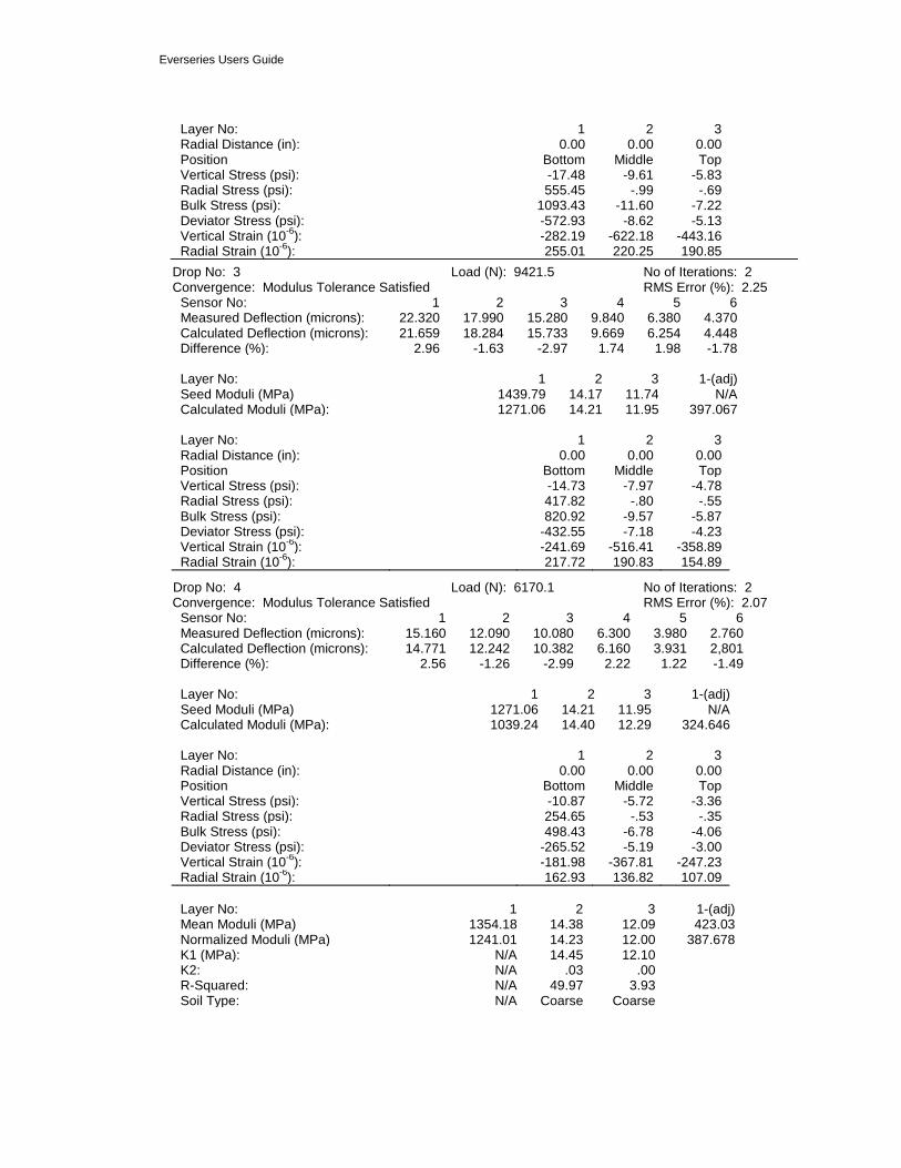
2.6.7.3 Backcalculation Results (No Stiff Layer)
BACKCALCULATION by Evercalc© 5.0 - Detail Output Route: Example No. 1 - No Stiff Layer Plate Radius (in): 5.9 No. of Layers: 3 No of Sensors: 6 Stiff Layer: No Offsets (in) .0.0 8.0 12.0 24.0 36.0 48.0 P-Ratio: .350 .400 .450 Station: 210 No of Drops: 4 Average RMS Error (%): 2.30 Thickness (in): 4.00 16.00 Pavement Temperature (F): 50.0 Drop No: 1 Load (N): 16717.7 No of Iterations: 5 Convergence: Modulus Tolerance Satisfied RMS Error (%): 2.73
Sensor No: 1 2 3 4 5 6 Measured Deflection (microns): 35.980 29.210 25.160 16.770 11.220 7.560 Calculated Deflection (microns): 34.678 29.791 25.998 16.550 10.873 7.731 Difference (%): 3.62 -1.99 -3.33 1.31 3.10 -2.26
Layer No: 1 2 3 1-(adj) Seed Moduli (MPa) 400.00 25.00 15.00 N/A Calculated Moduli (MPa): 1666.63 14.76 12.36 520.638
Layer No: 1 2 3 Radial Distance (in): 0.00 0.00 0.00 Position Bottom Middle Top Vertical Stress (psi): -22.91 -12.80 -7.86 Radial Stress (psi): 796.86 -1.41 -.98 Bulk Stress (psi): 1570.81 -15.62 -9.83 Deviator Stress (psi): -819.77 -11.39 -6.88 Vertical Strain (10-6): -348.43 -790.78 -564.76 Radial Strain (10-6): 315.59 289.57 242.65
Drop No: 2 Load (N): 12022.8 No of Iterations: 2 Convergence: Modulus Tolerance Satisfied RMS Error (%): 2.46
Sensor No: 1 2 3 4 5 6 Measured Deflection (microns): 27.800 22.600 19.290 12.720 8.390 5.710 Calculated Deflection (microns): 26.911 22.960 19.927 12.519 8.182 5.824 Difference (%): 3.20 -1.59 -3.30 1.58 2.47 -1.99
Layer No: 1 2 3 1-(adj) Seed Moduli (MPa) 1666.63 14.76 12.36 N/A Calculated Moduli (MPa): 1439.79 14.17 11.74 449.776
Everseries Users Guide
Layer No: 1 2 3 Radial Distance (in): 0.00 0.00 0.00 Position Bottom Middle Top Vertical Stress (psi): -17.48 -9.61 -5.83 Radial Stress (psi): 555.45 -.99 -.69 Bulk Stress (psi): 1093.43 -11.60 -7.22 Deviator Stress (psi): -572.93 -8.62 -5.13 Vertical Strain (10-6): -282.19 -622.18 -443.16 Radial Strain (10-6): 255.01 220.25 190.85
Drop No: 3 Load (N): 9421.5 No of Iterations: 2 Convergence: Modulus Tolerance Satisfied RMS Error (%): 2.25
Sensor No: 1 2 3 4 5 6 Measured Deflection (microns): 22.320 17.990 15.280 9.840 6.380 4.370 Calculated Deflection (microns): 21.659 18.284 15.733 9.669 6.254 4.448 Difference (%): 2.96 -1.63 -2.97 1.74 1.98 -1.78
Layer No: 1 2 3 1-(adj) Seed Moduli (MPa) 1439.79 14.17 11.74 N/A Calculated Moduli (MPa): 1271.06 14.21 11.95 397.067
Layer No: 1 2 3 Radial Distance (in): 0.00 0.00 0.00 Position Bottom Middle Top Vertical Stress (psi): -14.73 -7.97 -4.78 Radial Stress (psi): 417.82 -.80 -.55 Bulk Stress (psi): 820.92 -9.57 -5.87 Deviator Stress (psi): -432.55 -7.18 -4.23 Vertical Strain (10-6): -241.69 -516.41 -358.89 Radial Strain (10-6): 217.72 190.83 154.89
Drop No: 4 Load (N): 6170.1 No of Iterations: 2 Convergence: Modulus Tolerance Satisfied RMS Error (%): 2.07
Sensor No: 1 2 3 4 5 6 Measured Deflection (microns): 15.160 12.090 10.080 6.300 3.980 2.760 Calculated Deflection (microns): 14.771 12.242 10.382 6.160 3.931 2,801 Difference (%): 2.56 -1.26 -2.99 2.22 1.22 -1.49
Layer No: 1 2 3 1-(adj) Seed Moduli (MPa) 1271.06 14.21 11.95 N/A Calculated Moduli (MPa): 1039.24 14.40 12.29 324.646
Layer No: 1 2 3 Radial Distance (in): 0.00 0.00 0.00 Position Bottom Middle Top Vertical Stress (psi): -10.87 -5.72 -3.36 Radial Stress (psi): 254.65 -.53 -.35 Bulk Stress (psi): 498.43 -6.78 -4.06 Deviator Stress (psi): -265.52 -5.19 -3.00 Vertical Strain (10-6): -181.98 -367.81 -247.23 Radial Strain (10-6): 162.93 136.82 107.09 Layer No: 1 2 3 1-(adj) Mean Moduli (MPa) 1354.18 14.38 12.09 423.03 Normalized Moduli (MPa) 1241.01 14.23 12.00 387.678 K1 (MPa): N/A 14.45 12.10 K2: N/A .03 .00 R-Squared: N/A 49.97 3.93 Soil Type: N/A Coarse Coarse
Everseries Users Guide
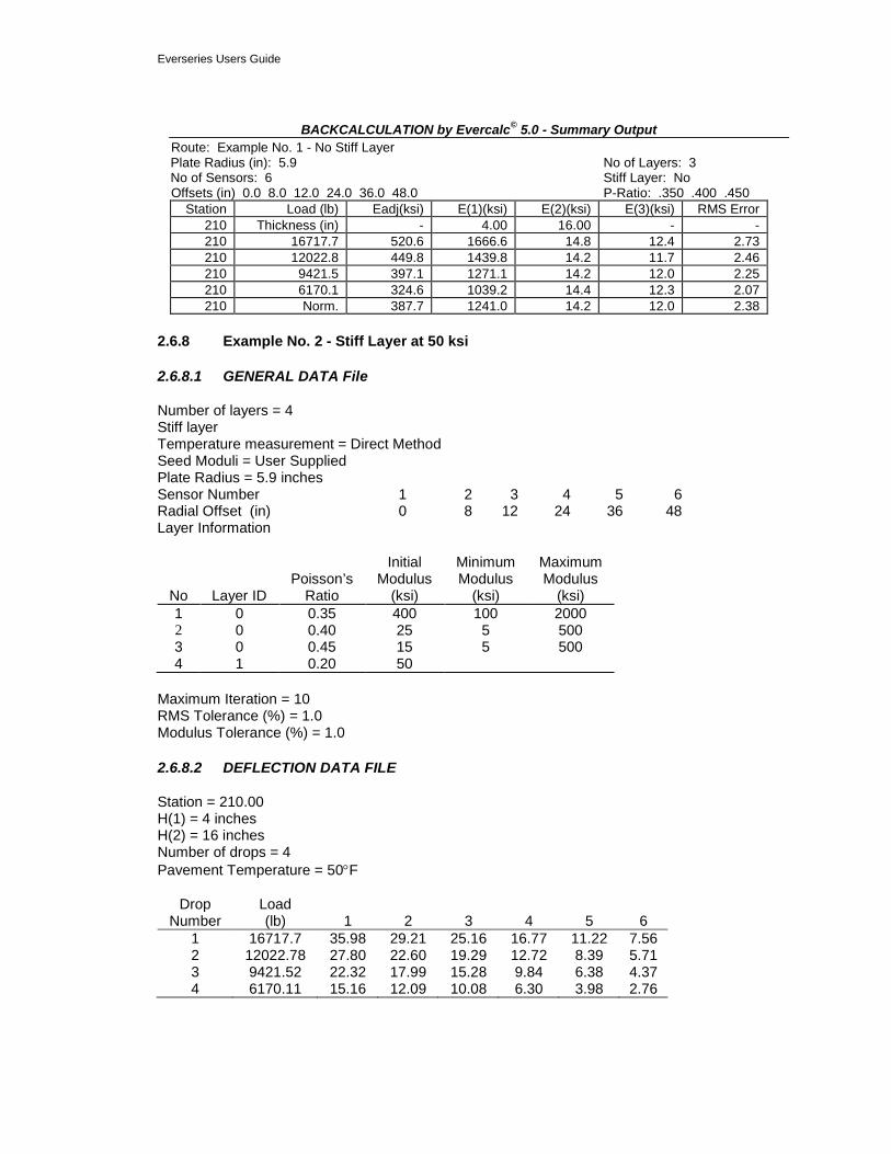
BACKCALCULATION by Evercalc© 5.0 - Summary Output Route: Example No. 1 - No Stiff Layer Plate Radius (in): 5.9 No of Layers: 3 No of Sensors: 6 Stiff Layer: No Offsets (in) 0.0 8.0 12.0 24.0 36.0 48.0 P-Ratio: .350 .400 .450
Station Load (lb) Eadj(ksi) E(1)(ksi) E(2)(ksi) E(3)(ksi) RMS Error 210 Thickness (in) - 4.00 16.00 - - 210 16717.7 520.6 1666.6 14.8 12.4 2.73 210 12022.8 449.8 1439.8 14.2 11.7 2.46 210 9421.5 397.1 1271.1 14.2 12.0 2.25 210 6170.1 324.6 1039.2 14.4 12.3 2.07 210 Norm. 387.7 1241.0 14.2 12.0 2.38
2.6.8 Example No. 2 - Stiff Layer at 50 ksi
2.6.8.1 GENERAL DATA File
Number of layers = 4 Stiff layer Temperature measurement = Direct Method Seed Moduli = User Supplied Plate Radius = 5.9 inches Sensor Number 1 2 3 4 5 6 Radial Offset (in) 0 8 12 24 36 48 Layer Information
Initial Minimum Maximum Poisson’s Modulus Modulus Modulus
No Layer ID Ratio (ksi) (ksi) (ksi) 1 0 0.35 400 100 2000 2 0 0.40 25 5 500 3 0 0.45 15 5 500 4 1 0.20 50
Maximum Iteration = 10 RMS Tolerance (%) = 1.0 Modulus Tolerance (%) = 1.0
2.6.8.2 DEFLECTION DATA FILE
Station = 210.00 H(1) = 4 inches H(2) = 16 inches Number of drops = 4 Pavement Temperature = 50°F
Drop Load Number (lb) 1 2 3 4 5 6
1 16717.7 35.98 29.21 25.16 16.77 11.22 7.56 2 12022.78 27.80 22.60 19.29 12.72 8.39 5.71 3 9421.52 22.32 17.99 15.28 9.84 6.38 4.37 4 6170.11 15.16 12.09 10.08 6.30 3.98 2.76

Everseries Users Guide
2.6.8.3 BACKCALCULATION RESULTS
BACKCALCULATION by Evercalc© 5.0 - Detail Output Route: Example No. 1 - Stiff Layer Plate Radius (in): 6.9 No. of Layers: 4 No of Sensors: 6 Stiff Layer: Yes Offsets (in) .0 8.0 12.0 24.0 36.0 48.0 P-Ratio: .350 .400 .450 .200 Station: 210 No of Drops: 4 Average RMS Error (%): 1.85 Thickness (in): 4.00 16.00 284.83 Pavement Temperature (F): 50.0 Drop No: 1 Load (lbf): 16717.7 No of Iterations: 5 Convergence: Modulus Tolerance Satisfied RMS Error (%): 2.23
Sensor No: 1 2 3 4 5 6 Measured Deflection (microns): 35.980 29.210 25.160 16.770 11.220 7.560 Calculated Deflection (microns): 35.031 29.744 25.806 16.474 10.955 7.719 Difference (%): 2.64 -1.83 -2.57 1.76 2.36 -2.10
Layer No: 1 2 3 4 1-(adj) Seed Moduli (MPa) 400.00 25.00 15.00 50.00 N/A Calculated Moduli (MPa): 1361.51 20.81 10.17 50.00 425.321
Layer No: 1 2 3 Radial Distance (in): 0.00 0.00 0.00 Position Bottom Middle Top Vertical Stress (psi): -30.10 -14.29 -7.42 Radial Stress (psi): 691.08 .31 -.58 Bulk Stress (psi): 1352.06 -13.67 -8.58 Deviator Stress (psi): -721.17 -14.60 -6.83 Vertical Strain (10-6): -377.41 -698.32 -677.40 Radial Strain (10-6): 337.67 283.48 296.51
Drop No: 2 Load (lbf): 12022.8 No of Iterations: 3 Convergence: Modulus Tolerance Satisfied RMS Error (%): 1.93
Sensor No: 1 2 3 4 5 6 Measured Deflection (microns): 27.800 22.600 19.290 12.720 8.390 5.710 Calculated Deflection (microns): 27.188 22.914 19.770 12.470 8.253 5.808 Difference (%): 2.20 -1.39 -2.54 1.97 1.63 -1.72
Layer No: 1 2 3 4 1-(adj) Seed Moduli (MPa) 1361.51 20.81 10.17 50.00 N/A Calculated Moduli (MPa): 1173.31 19.72 9.66 50.00 366.529
Layer No: 1 2 3 Radial Distance (in): 0.00 0.00 0.00 Position Bottom Middle Top Vertical Stress (psi): -22.81 -10.69 -5.48 Radial Stress (psi): 479.81 .25 -.41 Bulk Stress (psi): 936.81 -10.19 -6.31 Deviator Stress (psi): -502.63 -10.94 -5.07 Vertical Strain (10-6): -305.70 -552.22 -529.28 Radial Strain (10-6): 272.62 224.42 232.00
Drop No: 3 Load (lbf): 9421.5 No of Iterations: 2 Convergence: Modulus Tolerance Satisfied RMS Error (%): 1.70
Sensor No: 1 2 3 4 5 6 Measured Deflection (microns): 22.320 17.990 15.280 9.840 6.380 4.370 Calculated Deflection (microns): 21.879 18.240 15.604 9.640 6.315 4.430 Difference (%): 1.97 -1.39 -2.12 2.03 1.02 -1.36

Everseries Users Guide
Layer No: 1 2 3 4 1-(adj) Seed Moduli (MPa) 1173.31 19.72 9.66 50.00 N/A Calculated Moduli (MPa): 1041.23 19.28 9.89 50.00 325.270
Layer No: 1 2 3 Radial Distance (in): 0.00 0.00 0.00 Position Bottom Middle Top Vertical Stress (psi): -18.89 -8.80 -4.51 Radial Stress (psi): 361.37 .13 .33 Bulk Stress (psi): 703.85 -8.54 -5.16 Deviator Stress (psi): -380.27 -8.93 -4.18 Vertical Strain (10-6): -261.09 -462.02 -425.88 Radial Strain (10-6): 231.94 186.73 186.85
Drop No: 4 Load (lbf): 6170.1 No of Iterations: 2 Convergence: Modulus Tolerance Satisfied RMS Error (%): 1.51
Sensor No: 1 2 3 4 5 6 Measured Deflection (microns): 15.160 12.090 10.080 6.300 3.980 2.760 Calculated Deflection (microns): 14.927 12.204 10.287 6.151 3.977 2.783 Difference (%): 1.54 -.94 -2.06 2.36 0.7 -.84
Layer No: 1 2 3 4 1-(adj) Seed Moduli (MPa) 1041.23 19.28 9.89 50.00 N/A Calculated Moduli (MPa): 851.63 18.93 10.25 50.00 266.039
Layer No: 1 2 3 Radial Distance (in): 0.00 0.00 0.00 Position Bottom Middle Top Vertical Stress (psi): -13.68 -6.26 -3.17 Radial Stress (psi): 219.42 .05 -.21 Bulk Stress (psi): 425.15 -6.16 -3.60 Deviator Stress (psi): -233.09 -6.31 -2.96 Vertical Strain (10-6): -196.41 -332.97 -290.69 Radial Strain (10-6): 173.09 133.93 127.77 Layer No: 1 2 3 4 1-(adj) Mean Moduli (MPa) 1106.92 19.68 9.99 50.00 345.79 Normalized Moduli (MPa) 1016.65 19.23 9.93 50.00 317.591 K1 (MPa): N/A 20.36 9.80 N/A K2: N/A .15 -.02 N/A R-Squared: N/A 96.79 21.17 N/A Soil Type: N/A Coarse Fine N/A
BACKCALCULATION by Evercalc© 5.0 - Summary Output Route: Example No. 1 - Stiff Layer Plate Radius (in): 5.9 No of Layers: 4 No of Sensors: 6 Stiff Layer: Yes Offsets (in) 0.0 8.0 12.0 24.0 36.0 48.0 P-Ratio: .350 .400 .450 .200
Station Load (lbf) Eadj(ksi) E(1)(ksi) E(2)(ksi) E(3)(ksi) E(4)(ksi) RMS Error 210 Thickness (in) - 4.00 16.00 284.83 - - 210 16717.7 425.3 1361.5 20.8 10.2 50.0 2.23 210 12022.8 366.5 1173.3 19.7 9.7 50.0 1.93 210 9421.5 325.3 1041.2 19.3 9.9 50.0 1.70 210 6170.1 266.0 851.6 18.9 10.2 50.0 1.51 210 Norm. 317.6 1016.7 19.2 9.9 50.0 1.85

Everseries Users Guide
2.6.9 Example No. 2 - Stiff Layer at 50 ksi
From the summary outputs for the no stiff layer and stiff layer examples, the following normalized (9000 lb.) results show:
Example Eadj E1 E2 E3 RMSE No stiff layer 387.7 1241.0 14.2 12.0 2.38 Stiff layer 317.6 1016.7 19.2 9.9 1.85
From this summary both the no stiff and stiff layer examples provide reasonable results with low RMSE. With the lower base moduli, it appears that the base material may have been compromised (infiltrated with fine material) due to the low stiffness (weak) subgrade (field evaluation could be used to verify this result). Use of either result would be appropriate. However, the results of the stiff layer provide a lower RMSE and more realistic moduli for the base and subgrade moduli.

Everseries Users Guide
References
1 Michelow, J., Analysis of Stress and Displacements in an n-Layered Elastic System under a Load Uniformly Distributed on a Circular Area California Research Corporation, Richmond, California, 1963.
2 Lytton, R.L., "Backcalculation of Pavement Layer Properties," Nondestructive Testing of Pavements and Backcalculation of Moduli, ASTM STP 1026, American Society for Testing and Materials, Philadelphia, 1989, pp. 7-38.
3 Rhode, G. T. And Scullion, T., “MODULUS 4.0: Expansion and Validation of the Modulus Backcalculation System,” Research Report 1123-3, Texas Transportation Institute, Texas A&M University, College Station, Texas, November 1990.
4 Hossain, A.S.M., and Zaniewski, J.P., "Detection and Determination of Depth of Rigid Bottom in Backcalculation of Layer Moduli from Falling Weight Deflectometer Data," Transportation Research Record No. 1293, Transportation Research Board, Washington, D.C., 1991.
5 Winters, B.C., "The PACCAR Pavement Test Section — Instrumentation and Validation," Master's thesis, Department of Civil Engineering, University of Washington, Seattle, Washington, March 1993.
6 Lenngren, C.A., "Relating Bearing Capacity to Pavement Condition," Ph.D. Dissertation, Royal Institute of Technology, Department of Highway Engineering, Stockholm, Sweden, 1990.
7 Darter, M.I., Elliott, R.P., and Hall, K.T., "Revision of AASHTO Pavement Overlay Design Procedure," Project 20-7/39, National Cooperative Highway Research Program, Transportation Research Board, Washington, D.C., September 1991.
8 Newcomb, D. E., “Development and Evaluation of Regression Method to Interpret Dynamic Pavement Deflections,” Ph.D. Dissertation, Department of Civil Engineering, University of Washington, Seattle, Washington, 1986.
9 Bu-Bushait, A. A., “Development of a Flexible Pavement Fatigue Model for Washington State,” Ph.D. Dissertation, Department of Civil Engineering, University of Washington, Seattle, Washington, 1985.
10 The Asphalt Institute, Thickness Design — Asphalt Pavement for Highways and Streets, Manual Series No. 1 (MS-1), College Park, Maryland, September 1981.
11 Shook, J.F., Finn, F.N., Witczak, M.W., and Monismith, C.L., "Thickness Design of Asphalt Pavements — The Asphalt Institute Method," Proceedings, Fifth International Conference on the Structural Design of Asphalt Pavements, The Delft University of Technology, The Netherlands, 1982.
12 Monismith, C.L., and Epps, J.A., "Asphalt Mixture Behavior in Repeated Flexure," Institute of Transportation and Traffic Engineering, University of California, Berkeley, 1969.
13 Finn, F.N., et al., "The Use of Distress Prediction Subsystems for the Design of Pavement Structures," Proceedings, 4th International Conference on the Structural Design of Asphalt Pavements, University of Michigan, Ann Arbor, 1977.
14 Mahoney, J.P., Lee, S.W., Jackson, N.C., and Newcomb, D.E., "Mechanistic Based Overlay Design Procedure or Washington State Flexible Pavements," Research Report

Everseries Users Guide
WA-RD 170.1, Washington State Department of Transportation, Olympia, Washington, 1989.
15 Southgate, H. F., and Deen, R. C., “Temperature Distributions in Asphalt Concrete Pavements”, Highway Research Record No. 549, Highway Research Board, Washington, D.C., 1975, pp. 39-46.
16 Horak, E., "The Use of Surface Deflection Basin Measurements in the Mechanistic Analysis of Flexible Pavements," Proceedings, Vol. 1, Sixth International Conference Structural Design of Asphalt Pavements, University of Michigan, Ann Arbor, Michigan, USA, 1987.
17 The Asphalt Institute, "Asphalt Overlays for Highway and Street Pavement Rehabilitation," Manual Series No. 17, the Asphalt Institute, College Park, Maryland, June 1983.
18 Rutherford, M.S., Mahoney, J.P., Hicks, R.G., and Rwebangira, T., "Guidelines for Spring Highway Use Restrictions," Research Report WA-RD 80.1 (WSDOT) and FHWA-RD-86-501 (FHWA), August 1985.
19 Kono, F., Takahashi, T., Kubo, H. and Hiraoka, H., "Pavement Design in Cold Areas," Proceedings, Symposium on Frost Action on Roads, Norwegian Road Research Laboratory, Oslo, Norway, October 1973.

Everseries Users Guide
Appendix A – Nondestructive Testing Interpretation Techniques
Clearly, there are all kinds of NDT data which can be collected on or about pavements but concentration is placed on measured surface deflections.
DEFLECTION BASIN PARAMETERS
Over the years numerous techniques have been developed to analyze deflection data from various kinds of pavement deflection equipment. A fairly complete summary of deflection basin parameters was provided by Horak at the Sixth International Conference Structural Design of Asphalt Pavement [15] and is shown in Table A-1.
Table A-1. Summary of Deflection Basin Parameters [modified from 15]
Parameter Formula Measuring device
Maximum deflection D0 Benkelman Beam, Lacroux deflectometer, FWD
Radius of curvature )1D/D(D2rR
r00
2
−=
r = 5" Curvaturemeter
Spreadability
++
=+
0
3210
D100]5/)DDDD[(S
D1 … D3 spaced 12" apart
Dynaflect
Area )]D/D()D/D(2)D/D(21[6A 030221 +++=
0, 1, 2, 3 feet FWD
Shape factors F1 = (D0 -D2) / D1 F2 = (D1 -D3) / D2
FWD
Surface curvature index
SCI = D0 - Dr
where r = 12" or r = 20" Benkelman Beam Road Rater FWD
Base curvature index BCI = D24" - D36" Road Rater
Base damage index BDI = D12" - D24" Road Rater
Deflection ratio Qr = Dr/D0
where Dr = D0/2 FWD
Bending index BI = D/a where a = Deflection basin
Benkelman Beam
Slope of deflection SD = tan-1 (D0 - Dr)/r where r = 24 inches
Benkelman Beam
All of these parameters tend to focus on four major areas:
(a) Plate or center load deflection which represents the total defection of the pavement. This was obviously the first deflection parameter which came with the Benkelman Beam. It has been used for many years as the primary input for several overlay design procedures.
Everseries Users Guide
(b) The slope or deflection differences close to the load such as Radius of Curvature (R), Shape Factor (F1), and Surface Curvature Index (SCI). These parameters tend to reflect the relative stiffness of the bound or upper regions of the pavement section.
(c) The slope or deflection differences in the middle of the basin about 11.8 inches to 35.4 inches from the center of the load. These parameters tend to reflect the relative stiffness of the base or lower regions of the pavement section.
(d) The deflections toward the end of the basin. Deflections in this region relate quite well to the stiffness of the subgrade below the pavement surfacing.
The subsequent parameters to be presented were developed to provide a means of obtaining the resilient modulus values of the surfacing layers more easily or quickly than full backcalculation. In general, the success of these regression equations to predict the resilient modulus of the surfacing layers has been limited. There is a clear consensus; however, that the deflections measured beyond the primary effects of the load stress bulb relate quite well to the resilient modulus of the subgrade, (ESG).
AREA PARAMETER
Over the years WSDOT has found that the use of selected indices and algorithms provide a "good picture" of the relative conditions found throughout a project. This picture is very useful in performing backcalculation and may at times be used by themselves on projects with large variations in surfacing layers.
WSDOT is currently using deflections measured at the center of the test load combined with Area values and ESG computed from deflections measured at 24 inches presented in a linear plot to provide a visual picture of the conditions found along the length of any project (as illustrated in Figure A-1).
The Area value represents the normalized area of a slice taken through any deflection basin between the center of the test load and 3 feet. By normalized, it is meant that the area of the slice is divided by the deflection measured at the center of the test load, D0. Thus the Area value is the length of one side of a rectangle where the other side of the rectangle is D0. The actual area of the rectangle is equal to the area of the slice of the deflection basin between 0 and 3 feet.
The original Area equation is:
A = 6(D0 + 2D1 + 2D2 + D3)/D0
where D0 = surface deflection at center of test load, D1 = surface deflection at 1 foot, D2 = surface deflection at 2 feet, and D3 = surface deflection at 3 feet.
The approximate metric equivalent of this equation is:
A = 150(D0 + 2D300 + 2D600 + D900)/D0
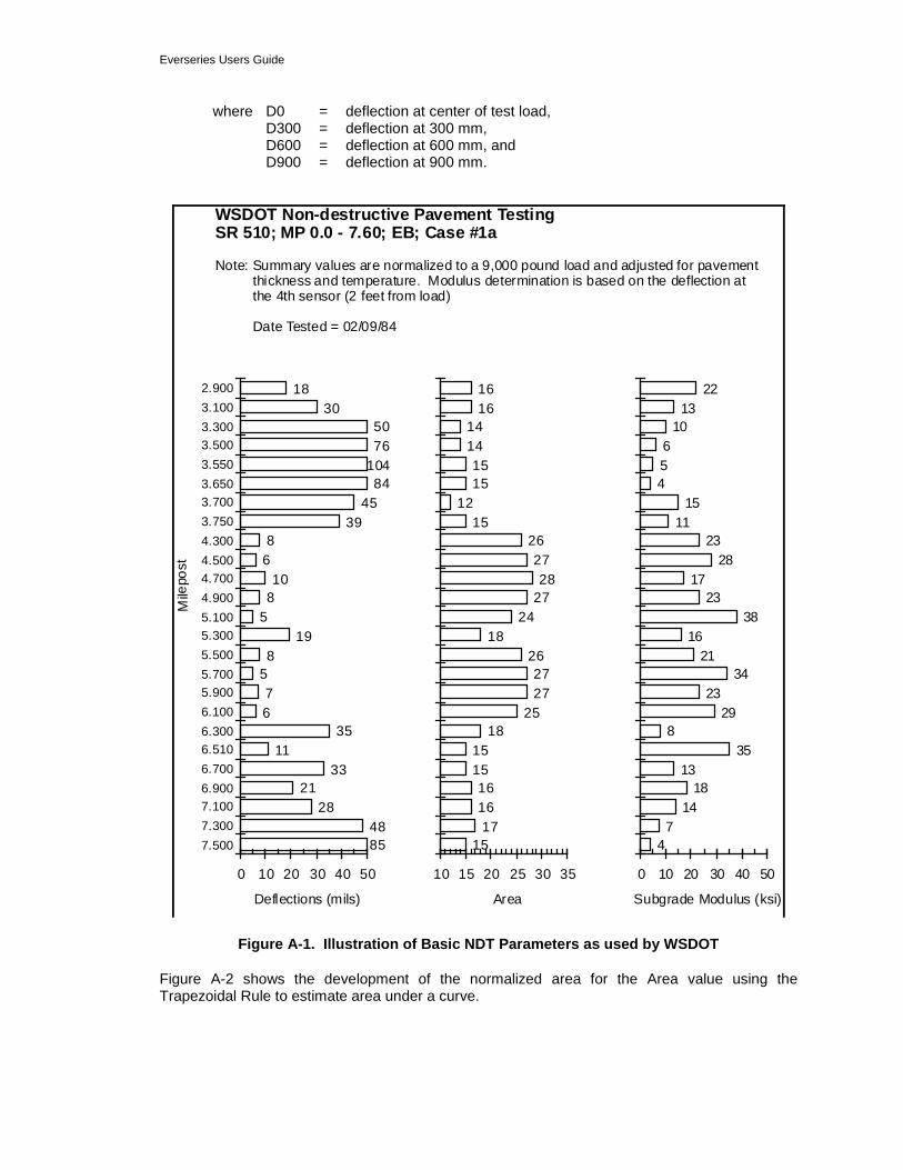
Everseries Users Guide
where D0 = deflection at center of test load, D300 = deflection at 300 mm, D600 = deflection at 600 mm, and D900 = deflection at 900 mm.
0 10 20 30 40 50
7.5007.3007.1006.9006.7006.5106.3006.1005.9005.7005.5005.3005.1004.9004.7004.5004.3003.7503.7003.6503.5503.5003.3003.1002.900
8548
2821
3311
3567
58
195810
68
3945
841047650
3018
10 15 20 25 30 35
1517
1616
1515
1825
2727
2618
242728
2726
1512
1515
1414
1616
0 10 20 30 40 50
47
1418
1335
829
2334
2116
3823
1728
2311
15456
1013
22
Mile
post
Deflections (mils) Area Subgrade Modulus (ksi)
WSDOT Non-destructive Pavement Testing SR 510; MP 0.0 - 7.60; EB; Case #1a Note: Summary values are normalized to a 9,000 pound load and adjusted for pavement
thickness and temperature. Modulus determination is based on the deflection at the 4th sensor (2 feet from load)
Date Tested = 02/09/84
Figure A-1. Illustration of Basic NDT Parameters as used by WSDOT
Figure A-2 shows the development of the normalized area for the Area value using the Trapezoidal Rule to estimate area under a curve.

Everseries Users Guide
0" 12" 24" 36"
D
= 0
.027
"0
D
= 0
.020
"1 D
= 0
.014
"2 D
= 0
.010
"3
D
= 0
.027
"0 D
=
0.0
20"
1
D
= 0
.014
"2
D
= 0
.010
"3
12"
12"6"
6"
D
= 0
.027
"0
A = 23.3
Typical Deflection Basin (Section B "Standard Pavement")
Estimated Area Using Trapezoidal Rule
Equal Area Bounded by D and Area Parameter
0
Figure A-2. Computing an Area Parameter
The basic Trapezoidal Rule is:
K = h
1
2y0 + y1 + y2 + 12y3
where K = any planar area, y0 = initial chord, y1, y2 = immediate chords, y3 = last chord, and h = common distance between chords.
Thus, to estimate the area of a deflected basin using D0, D1, D2, and D3, and h = 6 inches, then:
K = 6 (D0 + 2D1 + 2D2 + D3)
Everseries Users Guide
Further, normalize by dividing by D0:
Area = 6D0 (D0 + 2D1 + 2D2 + D3) or Area = 6 D0 + D3
D0
1 +2D1
D0 + 2D2
Thus, since we normalized by D0, the Area Parameter's unit of measure is inches (or mm) not in2 or mm2 as one might expect.
The maximum value for Area is 36.0 inches and occurs when all four deflection measurements are equal (not likely to actually occur) as follows:
If, D0 = D1 = D2 = D3
Then, Area = 6(1 + 2 + 2 + 1) = 36.0 inches
For all four deflection measurements to be equal (or nearly equal) would indicate an extremely stiff pavement system (like portland cement concrete slabs or thick, full-depth HMA.)
The minimum Area value should be no less than 11.1 inches.
This value can be calculated for a one-layer system which is analogous to testing (or deflecting) the top of the subgrade (i.e., no pavement structure). Using appropriate equations, the ratios of
D1D0
, D2D0
, D3D0
always result in 0.26, 0.125, and 0.083, respectively. Putting these ratios in the Area equation results in
Area = 6(1+ 2(0.26) + 2(0.125) + 0.083) = 11.1 inches
Further, this value of Area suggests that the elastic moduli of any pavement system would all be equal (e.g., E1 = E2 = E3 = …). This is highly unlikely for actual, in-service pavement structures. Low area values suggest that the pavement structure is not much different from the underlying subgrade material (this is not always a bad thing if the subgrade is extremely stiff — which doesn't occur very often).
Typical Area values were computed for pavement Sections A, B, and C (refer to Figure A-3) and are shown in Table A-2 (along with the calculated surface deflections (D0, D1, D2, D3)). The following provides a general guide in the use of Area values obtained from FWD pavement surface deflections.
Area Pavement (inch) (mm)
PCCP "Sound" PCC*
24-33 29-32
610-840 740-810
Thick HMA (≥ 0.35 feet) 21-30 530-760 Thin HMA (< 0.35 feet) 16-21 410-530 BST flexible pavement (relatively thin structure) 15-17 380-430 Weak BST 12-15 300-380

Everseries Users Guide
Section A (Thin Thickness Section)
2" (50 mm) ACP
6" (150 mm) Base
Fine-grained subgrade
5" (125 mm) ACP
8" (200 mm) Base
Fine-grained subgrade
9" (230 mm) ACP
6" (150 mm) Base
Fine-grained subgrade
Section B (Medium Thickness Section)
Section C (Thick Section)
Figure A-3. “Typical” Pavement Sections

Everseries Users Guide
Table A-2. Estimates of Area from Pavement Sections — Cases A, B, and C
Pavement Surface Deflections, inches
Pavement Cases D0 D1 D2 D3 Area
(inch) (mm) Standard Pavement Section A (thin) 0.048 0.026 0.014 0.009 17.1 (434) Section B (med) 0.027 0.020 0.014 0.010 23.3 (592) Section C (thick) 0.018 0.015 0.012 0.009 27.0 (686) Stabilize Subgrade Section A (thin) 0.036 0.020 0.013 0.009 18.5 (470) Section B (med) 0.023 0.017 0.012 0.009 23.5 (597) Section C (thick) 0.016 0.013 0.011 0.009 27.4 (696) Asphalt Treated Base Section A (thin) 0.021 0.018 0.013 0.010 26.6 (676) Section B (med) 0.014 0.012 0.010 0.009 28.7 (729) Section C (thick) 0.012 0.011 0.009 0.008 30.0 (762) Moisture Sensitivity Section A (thin) 0.053 0.026 0.014 0.009 16.1 (409) Section B (med) 0.033 0.022 0.014 0.009 20.7 (526) Section C (thick) 0.024 0.018 0.013 0.010 24.0 (610)
Table A-3. Trends of D0 and Area Values
FWD Based Parameter Area Maximum Surface
Deflection (D0) Generalized Conclusions*
Low Low Weak structure, strong subgrade
Low High Weak structure, weak subgrade
High Low Strong structure, strong subgrade
High High Strong structure, weak subgrade
*Naturally, exceptions can occur

Everseries Users Guide
Appendix B – Moduli Seasonal Variation
UNSTABILIZED MODULI
Based on FWD deflections obtained over a three-year period (1985 to 1987), the ratio of the moduli for the different seasons was estimated. These initial estimates are shown in Table C-1.
The data in Table C-1 suggest a greater variation in the base course (seasonally) than the subgrade. Clearly, this phenomenon can be quite site-specific. As such, the ratios are only, at best, "rules of thumb."
For dense graded base materials, numerous sources have suggested that moisture levels exceeding 85 percent of saturation can result in significant moduli reductions.
SEASONAL TEMPERATURES
Seasonal air temperatures are required inputs. These temperatures are used to adjust the AC moduli seasonally. These mean monthly air temperatures (MMAT) are converted to mean monthly pavement temperatures (MMPT) by use of the following equation:
MMPT = MMAT
1 +
1
z + 4 -
34
z + 4 + 6
where MMPT = mean monthly pavement temperature (°F), MMAT = mean monthly air temperature (°F), and z = depth below pavement surface (inch).
For example, if the MMAT = 65 °F and z = 3 inch, then
= (65)
1 +
1
3 + 4 -
34
3 + 4 + 6
= 75.4 °F

Everseries Users Guide
Table C-1. Design Moduli Ratios for Western and Eastern Washington Base Course and Subgrade Materials
1
Seasonal Period
Region Spring Summer Fall Winter Climate: Cool/Wet Warm/Dry Cool/Damp Cool/Wet Months: March June October December April July November January May August February
Western September Washington
Base 0.85 1.00 0.90 0.75 Subgrade 0.85 1.00 0.90 0.85 Climate: Thaw Hot/Dry Cool/Dry Freeze Months: February June October January March July November
Eastern April August December Washington May September
Base 0.65 1.00 0.90 1.10 Subgrade 0.90 1.00 0.90 1.10
1Design moduli ratios are appropriate for use if stress sensitive moduli relationships are not used. If stress sensitive moduli relationships are used (e.g., E = k1 θk2), then use of these ratios may overestimate seasonal effects.


![Everseries User Guide - References and Appendices · Everseries Users Guide References ... Manual Series No. 17, the Asphalt Institute, College Park, ... (D D D D ) / 5]100 S D1 …](https://static.fdocuments.us/doc/165x107/5c4287de93f3c338d2580f10/everseries-user-guide-references-and-everseries-users-guide-references-.jpg)