NATIONALCOOPERATIVE HIGHWAYRESEARCH PROGRAMNCHRP

REPORT 615

Evaluation of the Use and Effectiveness of

Wildlife Crossings

TRANSPORTATION RESEARCH BOARD 2008 EXECUTIVE COMMITTEE*

OFFICERS

CHAIR: Debra L. Miller, Secretary, Kansas DOT, Topeka VICE CHAIR: Adib K. Kanafani, Cahill Professor of Civil Engineering, University of California, Berkeley EXECUTIVE DIRECTOR: Robert E. Skinner, Jr., Transportation Research Board

MEMBERS

J. Barry Barker, Executive Director, Transit Authority of River City, Louisville, KYAllen D. Biehler, Secretary, Pennsylvania DOT, HarrisburgJohn D. Bowe, President, Americas Region, APL Limited, Oakland, CALarry L. Brown, Sr., Executive Director, Mississippi DOT, JacksonDeborah H. Butler, Executive Vice President, Planning, and CIO, Norfolk Southern Corporation, Norfolk, VAWilliam A.V. Clark, Professor, Department of Geography, University of California, Los AngelesDavid S. Ekern, Commissioner, Virginia DOT, RichmondNicholas J. Garber, Henry L. Kinnier Professor, Department of Civil Engineering, University of Virginia, CharlottesvilleJeffrey W. Hamiel, Executive Director, Metropolitan Airports Commission, Minneapolis, MNEdward A. (Ned) Helme, President, Center for Clean Air Policy, Washington, DCWill Kempton, Director, California DOT, SacramentoSusan Martinovich, Director, Nevada DOT, Carson CityMichael D. Meyer, Professor, School of Civil and Environmental Engineering, Georgia Institute of Technology, AtlantaMichael R. Morris, Director of Transportation, North Central Texas Council of Governments, ArlingtonNeil J. Pedersen, Administrator, Maryland State Highway Administration, BaltimorePete K. Rahn, Director, Missouri DOT, Jefferson CitySandra Rosenbloom, Professor of Planning, University of Arizona, TucsonTracy L. Rosser, Vice President, Corporate Traffic, Wal-Mart Stores, Inc., Bentonville, ARRosa Clausell Rountree, Executive Director, Georgia State Road and Tollway Authority, AtlantaHenry G. (Gerry) Schwartz, Jr., Chairman (retired), Jacobs/Sverdrup Civil, Inc., St. Louis, MOC. Michael Walton, Ernest H. Cockrell Centennial Chair in Engineering, University of Texas, AustinLinda S. Watson, CEO, LYNX–Central Florida Regional Transportation Authority, OrlandoSteve Williams, Chairman and CEO, Maverick Transportation, Inc., Little Rock, AR

EX OFFICIO MEMBERS

Thad Allen (Adm., U.S. Coast Guard), Commandant, U.S. Coast Guard, Washington, DCJoseph H. Boardman, Federal Railroad Administrator, U.S.DOTRebecca M. Brewster, President and COO, American Transportation Research Institute, Smyrna, GAPaul R. Brubaker, Research and Innovative Technology Administrator, U.S.DOTGeorge Bugliarello, Chancellor, Polytechnic University of New York, Brooklyn, and Foreign Secretary, National Academy of Engineering,

Washington, DCSean T. Connaughton, Maritime Administrator, U.S.DOTLeRoy Gishi, Chief, Division of Transportation, Bureau of Indian Affairs, U.S. Department of the Interior, Washington, DCEdward R. Hamberger, President and CEO, Association of American Railroads, Washington, DCJohn H. Hill, Federal Motor Carrier Safety Administrator, U.S.DOTJohn C. Horsley, Executive Director, American Association of State Highway and Transportation Officials, Washington, DCCarl T. Johnson, Pipeline and Hazardous Materials Safety Administrator, U.S.DOTJ. Edward Johnson, Director, Applied Science Directorate, National Aeronautics and Space Administration, John C. Stennis Space Center, MSWilliam W. Millar, President, American Public Transportation Association, Washington, DCNicole R. Nason, National Highway Traffic Safety Administrator, U.S.DOTJames Ray, Acting Administrator, Federal Highway Administration, U.S.DOT James S. Simpson, Federal Transit Administrator, U.S.DOTRobert A. Sturgell, Acting Administrator, Federal Aviation Administration, U.S.DOTRobert L. Van Antwerp (Lt. Gen., U.S. Army), Chief of Engineers and Commanding General, U.S. Army Corps of Engineers, Washington, DC

*Membership as of May 2008.

TRANSPORTAT ION RESEARCH BOARDWASHINGTON, D.C.

2008www.TRB.org

N A T I O N A L C O O P E R A T I V E H I G H W A Y R E S E A R C H P R O G R A M

NCHRP REPORT 615

Subject Areas

Planning and Administration • Energy and Environment • Highway and Facility Design • Maintenance

Evaluation of the Use and Effectiveness of

Wildlife Crossings

John A. BissonettePatricia C. Cramer

U.S. GEOLOGICAL SURVEY—UTAH COOPERATIVE FISH AND WILDLIFE RESEARCH UNIT

UTAH STATE UNIVERSITY

Logan, UT

Research sponsored by the American Association of State Highway and Transportation Officials in cooperation with the Federal Highway Administration

NATIONAL COOPERATIVE HIGHWAYRESEARCH PROGRAM

Systematic, well-designed research provides the most effective

approach to the solution of many problems facing highway

administrators and engineers. Often, highway problems are of local

interest and can best be studied by highway departments individually

or in cooperation with their state universities and others. However, the

accelerating growth of highway transportation develops increasingly

complex problems of wide interest to highway authorities. These

problems are best studied through a coordinated program of

cooperative research.

In recognition of these needs, the highway administrators of the

American Association of State Highway and Transportation Officials

initiated in 1962 an objective national highway research program

employing modern scientific techniques. This program is supported on

a continuing basis by funds from participating member states of the

Association and it receives the full cooperation and support of the

Federal Highway Administration, United States Department of

Transportation.

The Transportation Research Board of the National Academies was

requested by the Association to administer the research program

because of the Board’s recognized objectivity and understanding of

modern research practices. The Board is uniquely suited for this

purpose as it maintains an extensive committee structure from which

authorities on any highway transportation subject may be drawn; it

possesses avenues of communications and cooperation with federal,

state and local governmental agencies, universities, and industry; its

relationship to the National Research Council is an insurance of

objectivity; it maintains a full-time research correlation staff of

specialists in highway transportation matters to bring the findings of

research directly to those who are in a position to use them.

The program is developed on the basis of research needs identified

by chief administrators of the highway and transportation departments

and by committees of AASHTO. Each year, specific areas of research

needs to be included in the program are proposed to the National

Research Council and the Board by the American Association of State

Highway and Transportation Officials. Research projects to fulfill these

needs are defined by the Board, and qualified research agencies are

selected from those that have submitted proposals. Administration and

surveillance of research contracts are the responsibilities of the National

Research Council and the Transportation Research Board.

The needs for highway research are many, and the National

Cooperative Highway Research Program can make significant

contributions to the solution of highway transportation problems of

mutual concern to many responsible groups. The program, however, is

intended to complement rather than to substitute for or duplicate other

highway research programs.

Published reports of the

NATIONAL COOPERATIVE HIGHWAY RESEARCH PROGRAM

are available from:

Transportation Research BoardBusiness Office500 Fifth Street, NWWashington, DC 20001

and can be ordered through the Internet at:

http://www.national-academies.org/trb/bookstore

Printed in the United States of America

NCHRP REPORT 615

Project 25-27ISSN 0077-5614ISBN 978-0-309-11740-1Library of Congress Control Number 2008905372

© 2008 Transportation Research Board

COPYRIGHT PERMISSION

Authors herein are responsible for the authenticity of their materials and for obtainingwritten permissions from publishers or persons who own the copyright to any previouslypublished or copyrighted material used herein.

Cooperative Research Programs (CRP) grants permission to reproduce material in thispublication for classroom and not-for-profit purposes. Permission is given with theunderstanding that none of the material will be used to imply TRB, AASHTO, FAA, FHWA,FMCSA, FTA, or Transit Development Corporation endorsement of a particular product,method, or practice. It is expected that those reproducing the material in this document foreducational and not-for-profit uses will give appropriate acknowledgment of the source ofany reprinted or reproduced material. For other uses of the material, request permissionfrom CRP.

NOTICE

The project that is the subject of this report was a part of the National Cooperative HighwayResearch Program conducted by the Transportation Research Board with the approval ofthe Governing Board of the National Research Council. Such approval reflects theGoverning Board’s judgment that the program concerned is of national importance andappropriate with respect to both the purposes and resources of the National ResearchCouncil.

The members of the technical committee selected to monitor this project and to review thisreport were chosen for recognized scholarly competence and with due consideration for thebalance of disciplines appropriate to the project. The opinions and conclusions expressedor implied are those of the research agency that performed the research, and, while they havebeen accepted as appropriate by the technical committee, they are not necessarily those ofthe Transportation Research Board, the National Research Council, the AmericanAssociation of State Highway and Transportation Officials, or the Federal HighwayAdministration, U.S. Department of Transportation.

Each report is reviewed and accepted for publication by the technical committee accordingto procedures established and monitored by the Transportation Research Board ExecutiveCommittee and the Governing Board of the National Research Council.

The Transportation Research Board of the National Academies, the National ResearchCouncil, the Federal Highway Administration, the American Association of State Highwayand Transportation Officials, and the individual states participating in the NationalCooperative Highway Research Program do not endorse products or manufacturers. Tradeor manufacturers’ names appear herein solely because they are considered essential to theobject of this report.

CRP STAFF FOR NCHRP REPORT 615

Christopher W. Jenks, Director, Cooperative Research ProgramsCrawford F. Jencks, Deputy Director, Cooperative Research ProgramsChristopher J. Hedges, Senior Program OfficerEileen P. Delaney, Director of PublicationsNatalie Barnes, Editor

NCHRP PROJECT 25-27 PANELField of Transportation Planning—Area of Impact Analysis

J. M. Yowell, Versailles, KY (Chair)Kyle Williams, New York State DOT, Albany, NY Jason E. Alcott, Minnesota DOT, St. Paul, MN Brendan K. Chan, Ottawa, ON Kelly O. Cohen, California DOT, Sacramento, CA Michael W. Hubbard, Missouri Department of Conservation, Jefferson City, MO Jerald M. Powell, Lyons, CO Jodi R. Sivak, Gloucester, MA Mary E. Gray, FHWA Liaison Christine Gerencher, TRB Liaison

C O O P E R A T I V E R E S E A R C H P R O G R A M S

Cover photograph: Wolverine Overpass in Banff National Park, Alberta, Canada (© K. Gunson, used with permission).

AUTHOR ACKNOWLEDGMENTS

The research reported herein was conducted under NCHRP Project 25-27 by the U.S. Geological Sur-vey (USGS) Utah Cooperative Fish and Wildlife Research Unit, Department of Wildland Resources, Col-lege of Natural Resources at Utah State University (USU); Department of Civil Engineering, Ryerson Uni-versity; Engineering Professional Development Department, University of Wisconsin; Texas A&MUniversity; Sylvan Consulting Ltd., Invermere British Columbia, and Western Transportation Institute atMontana State University.

Utah State University was awarded the prime contract for this study. The work undertaken at the Uni-versity of Wisconsin, Texas A&M University, Ryerson University, Sylvan Consulting Ltd., and MontanaState University was performed under separate subcontracts with Utah State University. Principal inves-tigator for the effort is John A. Bissonette, Leader of the USGS Utah Cooperative Fish and WildlifeResearch Unit at Utah State University and Professor in the Department of Wildland Resources.

The work was done under the general supervision of Professor Bissonette with his Research AssociateDr. Patricia Cramer and his students Silvia Rosa and Carrie O’Brien at USU. Paul Jones, Jamey Anderson,Brian Jennings, Karen Wolfe, and Bill Adair at USU provided important technical help. The work at Ryer-son University was done under the supervision of Dr. Bhagwant Persaud with the assistance of Craig Lyon,Research Associate. The work at the University of Wisconsin and later at Texas A&M University was doneunder the supervision of Dr. Keith Knapp with the assistance of Ethan Shaw Schowalter-Hay. The workdone by Sylvan Consulting, Ltd. was accomplished by Nancy Newhouse and Trevor Kinley. Work per-formed at the Western Transportation Institute at Montana State University was done by Dr. AnthonyClevenger with the assistance of Amanda Hardy and Kari Gunson. Sandra Jacobson, Wildlife Biologist,U.S. Department of Agriculture Forest Service, Redwood Sciences Lab, Pacific Southwest Research Sta-tion, and Ingrid Brakop, Coordinator (former), Material Damage Loss Prevention, Insurance Corpora-tion of British Columbia, provided significant input to the evaluation of Task 3, and Ms. Jacobson pro-vided critical help with the Interactive Decision Guide.

Lead authors for report sections are as follows:

• Sections 2.2 and 2.3: Patricia C. Cramer and John A. Bissonette• Section 3.1: Keith Knapp, Bhagwant Persaud, Craig Lyon,

and Ethan Shaw Schowalter-Hay• Sections 3.2 and 3.3,

and Appendix E: Anthony P. Clevenger, Amanda Hardy, and Kari Gunson• Section 3.4: John A. Bissonette, Silvia Rosa, and Carrie O’Brien (Utah); Nancy Newhouse

and Trevor Kinley (British Columbia)• Sections 3.5 and 3.6: John A. Bissonette

We appreciate the access to the Kootenay River Ranch property provided by D. Hillary and T. Ennis ofthe Nature Conservancy of Canada. Research for the British Columbia segment of the study on the influ-ence of roads on small mammals (Section 3.4) was conducted under permit CB05-9954 issued by the BritishColumbia Ministry of Water, Land and Air Protection. Dr. H. Schwantje of the British Columbia Ministryof Water, Land and Air Protection was helpful in obtaining a provincial research permit. We thank C. Kassar,D. Ferreria, R. Klafki, T. McAllister, and H. Page for help with field work and species identification.

Many thanks to Bill Adair for his help with the hierarchical monothetic agglomerative clustering analy-sis discussed in Section 3.5.

The following list provides the affiliations of all authors who contributed to this report:

Utah State University, U.S. Geological Survey—Utah Cooperative Fish and Wildlife Research Unit

John A. BissonettePatricia C. CramerSilvia Rosa Carrie O’Brien Paul Jones Jamey Anderson Brian JenningsKaren G. Wolfe

Montana State UniversityAnthony P. ClevengerAmanda Hardy Kari Gunson

University of Wisconsin–MadisonKeith K. Knapp Ethan Shaw Schowalter-Hay

Ryerson UniversityBhagwant Persaud Craig Lyon

Sylvan Consulting, Ltd.Nancy Newhouse Trevor Kinley

U.S. Forest ServiceSandra Jacobson

Insurance Corporation of British ColumbiaIngrid Brakop

This report documents the development of an interactive, web-based decision guide pro-tocol for the selection, configuration, and location of wildlife crossings. For the first time,transportation planners and designers and wildlife ecologists have access to clearly written,structured guidelines to help reduce loss of property and life due to wildlife–vehicle colli-sions, while protecting wildlife and their habitat. The guidelines were based on goals andneeds identified and prioritized by transportation professionals from across North America,and developed using the results of five parallel scientific studies.

Every year, the costs of personal injuries and property damage resulting from wildlife–vehicle collisions are considerable and increasing. Various means have been employed tomitigate these collisions, with varying degrees of success. In recent years, highway agencieshave also placed a growing emphasis on protecting the environment. While many smallerspecies of animals do not pose a threat to vehicles through collisions, they experience sig-nificant habitat loss and fragmentation as a result of roadway alignments. Transportationcorridors limit the natural movement of wildlife, affecting individual species and eco-systems. There has been considerable research on the provision of wildlife crossings, butthere is a lack of data on their effectiveness and on the methods most effective for reducingwildlife–vehicle collisions and increasing landscape permeability for species in specific land-scapes. It also appears that crossings may work well for one species but not for others. Aninternational scan on wildlife habitat connectivity documented various strategies anddesigns used in Europe to improve the connectivity of wildlife habitats. Developing success-ful designs, methods, and strategies to make roadways more permeable to wildlife is but oneaspect of managing highways to avoid or minimize affects to the natural environment andmaintaining safety for motorists. This study was undertaken to provide state DOTs withguidance on the use and effectiveness of wildlife crossings to mitigate habitat fragmentationand reduce the number of animal–vehicle collisions on our roadways.

Under NCHRP Project 25-27, a research team led by John Bissonette and Patricia Cramerof Utah State University developed guidelines for the selection, configuration, location,monitoring, evaluation, and maintenance of wildlife crossings. The research was split intotwo phases. In the first phase, the team reviewed research and current practices, and con-ducted a survey of more than 400 respondents on existing wildlife crossings across theUnited States and Canada. In the second phase, a number of research studies were con-ducted: an analysis of wildlife–vehicle collision data, a study on the accuracy of spatialmodeling tools used to predict the influence of roadway geometry on wildlife–vehicle col-lisions, modeling of collision hotspots, a study on the influence of roads on small mammals,and an analysis of the spacing of crossings needed to restore fragmented habitat and migra-

F O R E W O R D

By Christopher J. HedgesStaff OfficerTransportation Research Board

tion patterns. Based on the results, the research team developed an interactive web-baseddecision guide protocol offering guidance on the selection, configuration, and location ofcrossing types, along with suggestions for their monitoring, evaluation, and maintenance.The decision tool is outlined in the report and can be found on the web at www.wildlifeandroads.org and on the AASHTO website (environment.transportation.org/environmental_issues/wildlife_roads/decision_guide/manual).

C O N T E N T S

1 Summary

10 Chapter 1 Introduction and Research Approach10 Introduction12 Research Approach13 Structure of the Report

15 Chapter 2 Phase 1 Summary15 2.1 Literature Search and Database15 2.2 The State of the Practice and Science of Wildlife Crossings

in North America15 Introduction16 Research Approach: Methods and Data16 Findings and Results16 Interpretation, Appraisal, and Applications20 Conclusions and Suggested Research21 2.3 Priorities in Research and Practice21 Introduction21 Research Approach: Methods and Data23 Findings and Results27 Interpretation, Appraisal, and Applications28 Conclusions and Suggested Research

30 Chapter 3 Phase 2 Segments30 3.1 Safety Data Analysis Aspects30 Introduction31 Research Approach: Methods and Data35 Findings and Results44 Interpretation, Appraisal, and Applications50 Conclusions and Suggested Research53 3.2 Limiting Effects of Roadkill Reporting Data Due to Spatial Inaccuracy53 Introduction53 Research Approach: Methods and Data57 Findings and Results59 Interpretation, Appraisal, and Applications62 Conclusions and Suggested Research62 3.3 Hotspots Modeling62 Introduction63 Research Approach: Methods and Data64 Findings and Results74 Interpretation, Appraisal, and Applications75 Conclusions

76 3.4 Influence of Roads on Small Mammals76 Introduction77 Research Approach: Methods and Data80 Findings and Results85 Interpretation, Appraisal, and Applications86 Conclusions86 3.5 Restoring Habitat Networks with Allometrically Scaled Wildlife Crossings86 Introduction87 Research Approach: Methods and Data90 Findings and Results93 Interpretation, Appraisal, and Applications94 Conclusions96 3.6 Interpretation of Research Results

98 Chapter 4 Decision Guide

110 References

118 Appendix A Priority Tables and Plan of Action

132 Appendix B Application of Safety Performance Functions in Other States or Time Periods

135 Appendix C Theoretical Background of Network Screeningfor Proportion Method

137 Appendix D Illustrating Regression to the Mean

139 Appendix E A Literature Review of Field Studies and Spatial Analyses for Hotspot Identificationof Wildlife–Vehicle Collisions

157 Appendix F Distance Sampling

159 Appendix G Allometric Scaling

S U M M A R Y

Introduction

Efforts at concerted and purposeful activity towards linking transportation services andecological services into a context-sensitive planning, construction, and monitoring processhave increased dramatically during the past few years. As a result, once piecemeal and hap-hazard mitigation approaches have been replaced with much more integrated efforts thathave provided useful data to highway planners and engineers. The research team for this proj-ect, NCHRP 25-27, “Evaluation of the Use and Effectiveness of Wildlife Crossings,” wascharged to provide guidance in the form of clearly written guidelines for the selection,configuration, and location of crossing types, as well as suggestions for the monitoring andevaluation of crossing effectiveness, and the maintenance of crossings. Providing guidanceon the use and effectiveness of wildlife crossings to mitigate habitat fragmentation and reducethe number of wildlife–vehicle collisions involves thinking in a large-scale, context-sensitiveframework that is based on sound ecological principles. Landscape permeability (i.e., the abil-ity for species to move freely across the landscape) is the guiding principle for this work, andthe foundation for effective mitigation. The goal for this research project was to developsound guidelines based on the premise that understanding and establishing landscape per-meability leads to effective landscape connectivity and the restoration of ecosystem integrity.At the same time, the guidelines should allow for efficient and effective transportation infra-structure mitigation in a cost-effective, economic manner. The guidelines were developed inthe form of a final report and a web-based interactive decision guide.

As a convention, the term “wildlife–vehicle collision” (WVC) is used rather than “animal–vehicle collision” (AVC), because this report is specifically dealing with only wildlife speciesand not domestic animals or livestock that may be hit by vehicles on the road. All other per-mutations, including for example, “wildlife crashes,” “WVC carcass collection,” and “wildlifecollisions,” are used rather than the more generic word “animal.” In Section 3.2, the term“ungulate–vehicle collision” is used because the data involved only hooved wildlife.

The research to accomplish the charge was carried out in two phases. In Phase 1, tworesearch efforts were completed. The first involved a North American telephone survey onthe state of the practice and research of wildlife crossings. The research team was able to doc-ument virtually all of the wildlife and aquatic crossings in the United States and Canada andto assemble information on them. The research team also reviewed studies that assess theefficacy of crossings and in doing so, learned what was working well. The second study ofPhase 1 was aimed at creating a continent-wide list of priority actions needed for practiceand research. The final list of top-ranked priorities was the result of the participation ofapproximately 444 professionals from across North America. In Phase 2, the research teamconducted five research efforts: (1) a safety research analysis of WVCs that included the

Evaluation of the Use and Effectivenessof Wildlife Crossings

1

2

development of Safety Performance Functions and an analysis of differences obtained whenusing WVC data versus deer carcass data, (2) an accuracy modeling effort that involved therelative importance of spatially accurate data, (3) an analysis that investigated the usefulnessof different kinds of clustering techniques to detect hotspots of wildlife killed on roads, (4) afield study of small mammals conducted in Utah and British Columbia that investigated theputative habitat degradation effects of roads, and (5) an investigation into allometric meth-ods to effectively place wildlife crossings to increase habitat permeability. Both Phase 1 and2 efforts provide linked and important data that were used to develop the web-based inter-active guidelines to inform decisions concerning wildlife crossings.

Clearly, transportation departments need reliable methods to identify WVC locations and toidentify potential mitigation measures, their placement, and their efficacy. The research devel-oped in this NCHRP project addressed all of these. There are serious methodological problemsassociated with current WVC research, so creating solutions requires the use of state-of-the-artmethods, such as predictive negative binomial models and empirical Bayes procedures. Thesestatistical methods can help to produce a widely accepted and usable guide that can be readilyapplied by Departments of Transportation. However, the choice of which database to use (e.g.,WVCs or carcass collection of wildlife road kills) to evaluate the WVC problem almost alwaysleads to the identification of different “hotspot” locations and ultimately different counter-measure improvements because (1) reported WVC data may represent only a small portion ofthe larger number of WVCs that occur 61,201 and (2) the spatial location accuracy of the datasetscan influence the validity of WVC models. The identification of collision-prone locations frommodel results is one step in the location of appropriate wildlife crossings.

To better identify potential mitigation measures for wildlife along transportation corridors,it is necessary to identify not only collision-prone zones, but also areas where landscapepermeability can be addressed for suites of species. Although crossings may be constructedbased in part on the WVC models and provide some measure of connectivity, landscape per-meability as experienced by the animal may not be achieved because of differences in move-ment ability among species. The allometric relationship between dispersal distances andhome range size of mammalian species can assist in deciding on the placement of wildlifecrossings that will help restore landscape permeability across fragmented habitat networks.The placement of wildlife crossings—in accordance with the movement needs of suites ofspecies, when used with additional information regarding hotspots of animal–vehicle colli-sions as well as dead animal counts on roads, along with appropriate auxiliary mitigation suchas exclusion fences and right-of-way escape structures—should significantly improve roadsafety as well as provide for easier movement of wildlife across the roaded landscape.

Even when wildlife crossings are appropriately placed, it is possible that road effects mayinclude habitat loss or degradation at some distance from the road, even though the roadedlandscape is permeable. It is necessary that mitigation efforts be evaluated for not only theirefficacy in reducing WVCs but also their ability in allowing multiple species to move acrossthe roaded landscape, thus promoting permeability.

The seven research efforts conducted in Phases 1 and 2 as part of NCHRP 25-27 addressedthese issues and provided usable data that helped in the development of the decision guide.The following sections provide the essential findings from each of the research efforts.

Phase 1 Results

Literature Review

The research team searched the literature pertaining to wildlife and roads and wildlife–vehicle collisions. The references were entered into the online database of literature for thisproject. The majority of references are annotated with key words and a description of the

research methods and results. There are more than 370 references in the database. URL ad-dresses for papers and reports that are posted on the internet are provided with the citationsin order to provide users maximum access to the literature. These references are accessiblefrom the search engine page of the Wildlife and Roads website (www.wildlifeandroads.org).

Wildlife Crossings Telephone Survey

The wildlife crossings research reported here is a summation of the North American tele-phone survey conducted to document as many known wildlife passages as possible in the UnitedStates and Canada. The telephone survey included participants employed by state/provincialand federal agencies, private organizations and companies, and academic institutions. Morethan 410 respondents answered questions concerning wildlife crossings, planning for wildlifeand ecosystems; WVC information; and past, current, and future research activities related toroads and wildlife.

The survey revealed 684 (663 U.S., 121 Canada) terrestrial and more than 10,692 (692+U.S., 10,000+ Canada) aquatic crossings in North America. These passages are found in 43of the United States and in 10 Canadian provinces and two territories. Trends found in thepractice of wildlife crossings included an increase in the number of target species in mitiga-tion projects, increasing numbers of endangered species as target species for mitigation,increasing involvement of municipal and state agencies, increasing placement of accompa-nying structures such as fencing and escape jump-out ramps, and a continent-wide neglectin maintenance of these structures. The trends in the science related to wildlife passagesincluded a greater tendency to monitor new passages for efficacy, a broadening of the num-ber of species studied, an increase in the length of monitoring time, increases in the numberof scientific partners conducting wildlife passage research, and increasingly sophisticatedresearch technology. The research team documented several projects in North America wherea series of crossings have been, or will be, installed to accommodate a suite of species and theirmovement needs, thus promoting permeability. A list of recommendations is presented toassist in the research, design, placement, monitoring, and maintenance of crossings. As anextension of the evaluation of the state of the science of wildlife crossings, the research teamreviewed studies that evaluated the use of wildlife passages. Approximately 25 scientific stud-ies assessed the efficacy of 70 terrestrial wildlife passages across North America and found thatall crossings passed wildlife; 68 passed the target wildlife species.

Gaps and Priorities

The research team developed a list of priorities related to wildlife and roadways andranked them based on the results of a web-based survey of U.S. and Canadian professionalsinvolved in transportation ecology. Initially, the research team developed a list of prioritiesbased on its knowledge of current research and practices in road safety and ecology. The pri-orities were developed and ranked to help direct research, policy, and management actionsacross North America that addressed the issue of reducing the impacts of the roaded land-scape on wildlife and ecosystem processes. The research team asked ecologists, engineers,and road-related professionals across North America to rank these priorities. The objectivewas to determine where additional research, field evaluations, and policy actions wereneeded to help maintain or restore landscape connectivity and permeability for wildlifeacross transportation corridors, while also minimizing wildlife–vehicle collisions. The list ofpriorities was initially reviewed and annotated by dozens of practitioners and researchers inNorth America and then ranked and annotated in surveys by persons attending two work-shops. The survey was refined and posted on the internet in April 2006, and potential

3

4

participants were invited to complete the survey by rating priorities. They were also askedto notify other qualified transportation and ecology professionals and invite them to takethe survey. The final list of ranked priorities was the result of the participation of 444professionals from across North America. The top five priorities were:

1. Incorporate wildlife mitigation needs early in the Department of Transportation(DOT)/Ministry of Transportation (MoT) programming, planning, and design process;

2. Better understand the dynamics of animal use of mitigation structures (e.g., what worksand what does not) and disseminate this information;

3. Combine several integrated animal-friendly mitigation methods such as wildlife cross-ings, fences, and escape ramps rather than relying on just one method;

4. Use conservation plans and connectivity analyses to inform the transportation pro-gramming/planning/design process on where mitigation is needed and how it may becarried out; and

5. Develop alternative cost-effective wildlife crossing designs and the principles upon whichthey are based.

Phase 2 Research Studies

Safety

The safety research involved analyses of WVC and road environment data from state DOTsources. Data were analyzed in two parts. In the first part, safety performance functions (SPFs)were calibrated for data on AVCs and road and traffic variables from four states; SPFs arepredictive models for WVCs that relate police-reported WVCs to traffic volume and road en-vironment data (geometrics) usually available in DOT databases. For each state, three levels ofSPFs were developed with varying data requirements. The first level required only the lengthand annual average daily traffic volume (AADT) of a road segment (a section of road, gener-ally between significant intersections and having essentially common geometric characteris-tics). The second level required road segments to be classified as flat, rolling, or mountainousterrain. The third level SPFs included additional roadway variables such as average lane width.SPF functions relate police-reported AVCs to traffic volume and road environment datausually available in DOT databases. (Police-reported AVCs include domestic animals as wellas wildlife, hence the use of the term “AVC” to characterize these reports. Only WVCs wereused in the analyses.)

Three SPF applications most relevant to the development of the desired guidelines for thisproject are included in this report: (1) network screening to identify roadway segments thatmay be good candidates for WVC countermeasures, (2) the evaluation of the effectivenessof implemented countermeasures, and (3) methodology for estimating the effectiveness ofpotential countermeasures. In general, the calibrated SPFs make good intuitive sense in thatthe sign, and to some extent the magnitude, of the estimated coefficients and exponents arein accord with expectations.

Surprisingly, the exponent of the AADT term, although reasonably consistent for thethree levels of models in a state, varied considerably across states and across facility types,reflecting differences in traffic operating conditions. The most significant variable found wasAADT. For application in another state, or even for application in the same four states fordifferent years to those in the calibration data, model recalibration is necessary to reflect dif-ferences across time and space for factors such as collision reporting practices, weather,driver demographics, and wildlife movements. In essence, a multiplier is estimated to reflectthese differences by first using the models to predict the number of collisions for a sample

5

of sites for the new state or time period. The sum of the collisions for those sites is dividedby the sum of the model predictions to derive the multiplier.

In deciding which of the four models is best to adopt for another state, it is necessary toconduct goodness-of-fit tests. Choosing the most appropriate model is especially importantbecause the exponents for AADT, by far the most dominant variable, differ so much betweenstates. A discussion of these tests is provided in a recent FHWA report.61 Additional sup-porting information is presented in the appendices.

The second part of the research effort involved an evaluation of the hypothesis that themagnitude and patterns of reported WVC data differed from the magnitude and patterns ofdeer carcass removal data as they typically exist at a DOT. These two types of data have beenused in the past, but their differences could lead to varying and possibly ineffective/ineffi-cient WVC-related policy and countermeasure decision making. Reported AVCs (whichtypically are provided by state highway safety enforcement agencies in crash reports) anddeer carcass removal locations (which are provided by highway maintenance crews in theirdaily activity reports) were acquired from Iowa and plotted within a geographic informa-tion system (GIS) platform. The spatial patterns of the two types of data were clearly differ-ent, and their calculated safety measures (e.g., average frequencies) varied. The use of theGIS plots, safety measures, or predictive models developed as part of this project could,therefore, lead to different WVC-related policies and countermeasure implementation andevaluation decisions. The choice of the database used to define and evaluate the WVC prob-lem and its potential countermeasures should be considered carefully. Recommendationsare provided regarding how the databases might be used appropriately and how the datawould be most profitably collected.

Accuracy Modeling

The accuracy modeling involved an investigation into the relative importance of factorsassociated with wildlife killed on the road. Two different datasets were used: one based onhigh-resolution, spatially accurate location data for carcasses along the roadside (<3 m error)representing an ideal situation and a second dataset created from the first that was charac-terized by lower resolution (high spatial error: ≤ 0.5 mi or 800 m, i.e., mile-marker data) andis likely typical of most transportation agency data. The goal of this research was to sum-marize how well these models identify landscape- and road-geometrics–based causes ofWVCs.

In this research, ungulate carcass datasets were used; the primary results of the analyses wereungulate–vehicle collision (UVC) models. The high-resolution, spatially accurate model hadhigher predictive power in identifying factors that contributed to collisions than the lower res-olution model based on mile-marker locations. Perhaps more noteworthy from this exercisewas the vast difference in predictive ability between the models developed with spatially accu-rate data versus the less accurate data obtained from referencing UVCs to a mile-markersystem. Besides learning about the parameters that contribute to UVCs in the study area, theresearch team discovered that spatially accurate data do make a difference in the ability ofmodels to provide not just statistically significant results, but more importantly, biologicallymeaningful results for transportation and resource managers responsible for reducing UVCsand improving motorist safety. The results have important implications for transportationagencies that may be analyzing data that have been referenced to a mile-marker system orunknowingly analyzing data that are spatially inaccurate. These findings lend support to thedevelopment of a national standard for the recording of WVCs and carcass locations, as wellas further research into new technologies that will enable transportation agencies to collectdata that are more accurate. Use of personal data assistants (PDAs) in combination with a

6

global positioning system (GPS) for routine highway maintenance activities126 can help agen-cies collect more spatially accurate and standardized data that will eventually lead to more in-formed analyses for transportation decision making.

This project also investigated the types of variables that explain WVCs, in particularwhether they are associated with landscape and habitat characteristics or physical featuresof the road itself. In two different types of analyses, the research team identified that vari-ables related to landscape and habitat were more significant than variables related to roadcharacteristics. Through this project, the research team demonstrated how WVC data canbe used to aid transportation management decision making and mitigation planning forwildlife.

Hotspot Modeling

The hotspot analysis used carcass data from wildlife killed on roads to investigate severalhotspot identification clustering techniques within a GIS framework that can be used in avariety of landscapes. These techniques take into account different scales of application andtransportation management concerns such as motorist safety and endangered species man-agement. Wildlife carcass datasets were obtained from two locations in North America withdifferent wildlife communities, landscapes, and transport planning issues. The research teamdemonstrated how this information can be used to identify WVC hotspots at different scalesof application, from project-level to state-level analysis. Some clustering techniques thatwere tested included Ripley’s K-statistic of roadkills, nearest neighbor measurements, anddensity measures. An overview of software applications that facilitate these types of analy-ses is provided.

In summary, data on hotspots of WVCs can aid transportation managers to increasemotorist safety or habitat connectivity for wildlife by providing safe passage across busyroadways. Knowledge of the geographic location and severity of WVCs is a prerequisitefor devising mitigation schemes that can be incorporated into future infrastructure proj-ects (bridge reconstruction, highway expansion). Hotspots in proximity to existing below-grade wildlife passages can help inform construction of structural retrofits that can helpkeep wildlife off roadways and increase habitat connectivity.

Influence of Roads on Small Mammals

The small-mammal research in this study involved an assessment of the potential of roadsto affect the abundance and distribution of small mammals by possible habitat degradation.The research team investigated what influence, if any, highways had on the relative abun-dance of small mammals and how far any observed effect might extend into adjacent habitat.Field studies along highways in both Utah and British Columbia were conducted.

In Utah, the research team captured 484 individuals of 13 species. The results showed dif-ferent trends of species diversity at different distances from the road from one year to the next.During 2004, the diversity of species was highest further from the road in direct contrast to2005, when diversity was highest closest to the road. Density and abundance data also differedbetween years and species. When the research team compared density in three distinct areas,sites with higher habitat quality (i.e., with greater forb and grass presence) had significantlyhigher small-mammal densities. Overall, it appeared that roads per se had little effect onsmall-mammal density. Rather, microhabitat conditions that were most favorable for eachindividual species appeared to be most responsible for density responses.

The results were similar for British Columbia, where the research team captured 401 indi-viduals of 11 species. Our results indicated that highway and transmission-line rights-of-way

(ROWs) appeared to be negative influences on abundance for most species and potentiallyneutral to positive for others. There were no consistent patterns in species abundance as thedistance in a forest increased from the road right-of-way. There was however, a consistentpattern of lower total species diversity in the road rights-of-way. Microhabitats and local con-ditions that varied among sites and transects and that remain independent of road or ROWappeared to be stronger than, or at least mask, any effects related to the road or ROW. For themost common and most habitat-generalist species, the deer mouse (Peromyscus maniculatus),there were no strong indications of an effect of distance from the highway or transmission line.Additionally, there was no evidence of any effect attributable to the highway that was notevident at the transmission-line sites. Impacts due to the highway itself may exist forsome species, but large samples and highly consistent habitat conditions would be required todetect them.

Restoring Habitat Networks with Allometrically Scaled Wildlife Crossings

In the research of allometric placement of crossings, the research team investigatedwhether differences in vagility (i.e., the natural ability of mammal species to move across thelandscape) could be used in deciding on the spacing of wildlife crossings that will help re-store landscape permeability across fragmented habitat networks. Until now, the placementof crossings has not been grounded in theory but has relied on empirical data to underpincrossing placement decisions, in part because the idea of landscape permeability has notbeen traditionally viewed from an animal perspective. When landscape permeability isviewed from an animal perspective, inherent species-specific movement capabilities providethe basis for developing scaling relationships (i.e., allometry) to inform the placement ofcrossings. In other words, the animals “tell” us where to place the crossings. There have beenuseful developments in allometric scaling laws that have led to important and statisticallysound relationships between home range size and dispersal distance for species. The recentlydescribed implications of the relationship of median dispersal distance (MedDD) to homerange area and the development of a single metric, termed the “linear home range distance”(LHRD), to represent home range size provide scaling laws that can be related to the con-cepts of ecological neighborhoods and domains of scale to consider how the movement ofspecies with similar movement capabilities can be enhanced by effective placement of cross-ings in roaded landscapes. In turn, this effective placement should reduce barrier effects andimprove permeability across habitat networks. It is possible to use MedDD as the upperbound and a LHRD as the lower bound to develop alternative domains of scale for groupsof animals to guide the placement of wildlife crossings.

The correct spacing of crossings is perhaps most urgent for large terrestrial mammals that,when involved in WVCs, tend to cause greater vehicle damage and have greater potential tocause human injury and death than smaller bodied animals. Large-bodied animals pose agreater safety risk. It appears that, to achieve the kind of landscape permeability that will helpensure the health of large-mammal populations (i.e., deer, moose, elk, and bear) and to min-imize WVCs, placement of wildlife crossings in areas where populations of these animals existwill entail at least a multistep decision process. The first step involves deciding which allomet-ric scaling domain is appropriate and feasible. Highest permeability will be obtained whencrossings of appropriate type and design are placed using the LHRD domains. If crossings wereplaced according to the MedDD, they would be too far apart to create high permeability of thelandscape. For example, using LHRD domains, wildlife crossings for white-tailed deer andmule deer would be placed at about 1 mi (1.6 km) apart in areas where these animals cross theroad frequently and are often hit by vehicles, which would certainly improve highway safety

7

8

and help ensure ease of movement, thus improving landscape permeability for these animals.Using the MedDD values of 6.1 to 7.4 mi to space the crossings is clearly inappropriate andwill do little to facilitate movement, especially if exclusion fencing is part of the mitigation.Similar arguments are appropriate for all species in general.

The use of allometric scaling domains represents only the first step to inform the place-ment and spacing of wildlife crossings. Additional local information including (1) locationof migration pathways, (2) knowledge of areas of local animal movement across roads, and(3) hotspots of WVC locations as well as dead animal count locations are needed. Whenthese data are used in an integrated and context-sensitive mitigation, these measures shouldhelp ensure landscape permeability, providing for easier movement across the roaded land-scape, and significantly improve highway safety.

Interpretation of Phase 2 Research Results

The sections on safety data analysis (3.1), accuracy modeling (3.2), and hotspot model-ing (3.3) address different ways to achieve similar purposes and therefore may be confusingfor the reader. The following paragraphs should help guide the reader in understanding thedistinctions.

The safety research (Section 3.1) is most effectively used when the purpose is to assess ifa specific mitigation has been successful in reducing WVCs to improve public safety. Thesafety approach has several applications and can be used to:

• Identify collision-prone locations for existing or proposed roads for all collision types com-bined or for specific target collision types

• Aid in the evaluation, selection, and prioritization of potential mitigation measures; and• Evaluate the effectiveness of mitigation measures already implemented.

An important caveat is that the safety approach does not address any aspect of wildlifepopulation response. As the models stand, their primary application is for the safety man-agement of existing roads as opposed to design or planning applications for new or newlybuilt roads. Significantly, the before-after analysis may be judged as successful from a roadsafety perspective, while at the same time the wildlife population concerned may be signifi-cantly reduced.

A second aspect of the safety effort clearly showed that the choice of the database used todefine and evaluate the WVC problem impacts whether a particular roadway segment mightbe identified for closer consideration and therefore the choice should be made carefully.Recommendations are provided in this report about how the databases might be usedappropriately and how the data can be most profitably collected.

In the accuracy modeling (Section 3.2), non-road-related variables (i.e., ecological fieldvariables, distance-to-landscape-feature variables, and GIS-generated buffer variables) wereassessed to determine their relative importance in explaining where ungulates were killed onthe road. Also, spatially accurate data were discovered to make a difference in the ability ofmodels to provide not just statistically significant results but more importantly, biologicallymeaningful results for transportation and resource managers responsible for reducingWVCs and improving motorist safety. Hence, these models are especially applicable whenit is important to locate hotspot areas of WVCs and hence wildlife crossings during thedesign and planning of new roads.

The hotspot analysis (Section 3.3) investigated WVC hotspot identification techniques,taking into account different scales of application and transportation management con-cerns. Simple plotting most often results in collision points being tightly packed together, in

some cases directly overlapping with neighboring WVC carcass locations, thus making itdifficult to identify distinct clusters, i.e., where the real high-risk collision areas occurred.Modeling or analytical techniques permit a more detailed assessment of where WVCs occur,their intensity, and the means to begin prioritizing highway segments for potential mitiga-tion applications.

The Ripley’s K analysis clearly shows the spatial distribution of WVCs and the importanceof broad-scale landscape variables (such as elevation and valley bottoms in a mountain en-vironment). Further, the locations of high-intensity roadkill clustering within each area canhelp to focus or prioritize the placement of mitigation activities, such as wildlife crossingsor other countermeasures, on each highway segment. The research team found that thenearest neighbor (CrimeStat®) approach was useful for identifying key hotspot areas onhighways with many roadkills because it, in essence, filters through the roadkill data to ex-tract where the most problematic areas lay. The density analysis approach identified morehotspot clusters on longer sections of highway. Although the density analysis approachappears to be less useful to management, it may be a preferred option where managers areinterested in taking a broader, more comprehensive view of wildlife–vehicle conflicts withina given area. Such a broader view may be necessary not only to prioritize areas of conflictsbut also to plan a suite of mitigation measures. The location of the larger clusters producedby the density analysis could be tracked each year to determine how stable they are orwhether there is a notable amount of shifting between years or over longer time periods. Thistype of information will be of value to managers in addressing the type of mitigation andintended duration (e.g., short-term vs. long-term applications).

The WVC data that transportation departments currently possess are suitable for meet-ing the primary objective of identifying hotspot locations at a range of geographic scales,from project-level (< 50 km of highway) to larger district-level or state-wide assessments onlarger highway network systems. The spatial accuracy of WVCs is not of critical importancefor the relatively coarse-scale analysis of where hotspots are located. Any of the analyticalclustering techniques can be used when more detailed information is needed.

9

10

Introduction

“For a generation, North Americans have been in simul-taneous pursuit of twin goals that are inherently in conflict.On the one hand, they seek to harvest the manifold benefitsof an expanding road system, including a strong economy,more jobs, and better access to schools, friends, family,recreation, and cheaper land on which to build ever largerhomes. On the other, they have growing concerns aboutthreats to the natural environment, including air and waterquality, wildlife habitat, loss of species, and expandingurban encroachment on rural landscapes. . . . Not surpris-ingly, these conflicting demands clash wherever transporta-tion decisions are made, whether at the federal, state, orlocal levels. . . . ad hoc environmental analysis has left manygaps in our understanding of effective mitigation forindividual road projects and is unlikely to ever lead to ef-fective mitigation of the macro effects of a growing systemof roads.”

Thomas B. Deen, Executive Director (retired)Transportation Research Board, National

Academy of SciencesMember, National Academy of Engineering

Foreword to Road Ecology: Science and Solutions98

“In the past century, dramatic changes have been made inthe U.S. road system to accommodate an evolving set ofneeds, including personal travel, economic development,and military transport. As the struggle to accommodatelarger volumes of traffic continues, the road system is in-creasing in width and, at a slower pace, overall length. As theroad system changes, so does the relationship between roadsand the environment. With the increase in roads, moreresources are going toward road construction and manage-ment. More is also understood about the impact of roads onthe environment. To address these matters, a better under-standing of road ecology and better methods of integrating

that understanding into all aspects of road development areneeded.”

Dr. Lance Gunderson (chair)Committee on Ecological Impacts of Road

Density, National Research CouncilPreface to Assessing and Managing the Ecological

Impacts of Paved Roads181

“My visions for the future are as follows. Road design infuture will commence with selection of routes with least eco-logical impacts. Wildlife bridges and tunnels will be locatedand built to minimum standards. There will be ecologicalrestoration of roadside verges.

“For every square metre of road there will be at least theequivalent of land set aside for nature. Roads will becomelinear nature reserves with hedgerows of native species and awide swathe on either side as a nature reserve. These linearnature reserves will be habitats for rare and endangeredspecies. Roadside verges will be enjoyed by all and traffic willslow to allow travelers to enjoy roadside nature.”

Dr. Ian F. Spellerberg, Professor of Nature ConservationLincoln University, Aotearoa, New Zealand

Chapter 8 of Ecological Effects of Roads217

These remarks suggest that transportation services andenvironmental concerns need to be effectively linked in alandscape context-sensitive planning, construction, andmonitoring process. They also provide an optimistic visionof the future, given the concerted efforts and purposeful ac-tivity towards linking transportation services and ecologicalservices that have increased dramatically during the past fewyears. For decades, environmental mitigation was not con-sidered an integral part of road construction and piecemealand haphazard mitigation approaches did not provide high-way planners and engineers with useful data that could begeneralized to different situations. However, following thecompletion of the interstate highway system, a new post-

C H A P T E R 1

Introduction and Research Approach

11

interstate era began with the passage of the Intermodal Sur-face Transportation Efficiency Act of 1991 (ISTEA), whicheffectively shifted responsibilities and funding from nationalpriorities to local needs and greater state and local govern-ment authority, while at the same time placing greater em-phasis on environmental mitigation and enhancement.98 In1998, the Transportation Equity Act for the 21st Century(TEA-21) retained this basic emphasis. The 2005 Safe, Ac-countable, Flexible, Efficient Transportation Equity Act: aLegacy for Users (SAFETEA-LU) continued this move to-ward environmental mitigation and gave even greater im-portance to facilitating both terrestrial and aquatic passageof wildlife, while also instructing that when metropolitanplans and statewide plans for transportation are developed,they must include “a discussion of potential environmentalmitigation activities and potential areas to carry out theseactivities” (SAFETEA-LU, Public Law 109-59, Title VI,Sec.6001 Transportation Planning Transportation Bill [Con-servation provisions of interest in SAFETEA-LU found at Defenders of Wildlife site: www.defenders.org/habitat/highways/safetea/; to read the text of the bill, see frwebgate.access.gpo.gov/cgi-bin/getdoc.cgi?dbname=109_cong_public_laws&docid=f:publ059.109]).

In Canada, Transport Canada published Road SafetyVision 2010, which calls for decreases of 30% in the num-ber of motorists killed or seriously injured. Over the lastdecade, legislation and policy including the National ParksAct and the Parks Canada Policy document have placed thehighest priority on the protection of ecological integrity,and include mitigation for wildlife on upgrades to high-ways within National Parks. Additionally, the recentSpecies at Risk Act in Canada has made planning and mit-igation for WVCs even more critical a concern for highwayplanners and engineers. Given the mandate of these majorlegislative acts, highway planners and engineers across theUnited States and Canada have begun to integrate mitiga-tion as part of their mandate. For example, British Colum-bia has developed a 10-year strategic plan to reduce wildlifecollisions by 50%. However, even with forward-looking ac-tions and excellent reports such as Assessing and Managingthe Ecological Impacts of Paved Roads181 and a large litera-ture on ecological “road effects,” there remains an obviouslack of synthesis documents to inform and help guide high-way planners and engineers with environmental mitigationand enhancement. Linking transportation and ecologicalservices effectively requires an integrated understanding ofthe science so that mitigation practices may be based ondata.

Historically, linking transportation and ecological servicesmay have seemed inherently in conflict but they need not beso. One can envision roads as having a physical and a virtualfootprint. The physical footprint is easy to see and includes

the actual dimensions of the road (length and width) as wellas the dimensions of associated structures, e.g., the right-of-way. The virtual footprint is much larger and includes thearea where the indirect effects of roads are manifested. Theroaded landscape has both direct and indirect effects onwildlife species, community biodiversity, and ecosystemhealth and integrity. The most prevalent direct effect is road-kill. Indirect effects include habitat loss, reduced habitat qual-ity, fragmentation, barrier effects, and loss of connectivityresulting in restricted or changed animal movement patterns.The virtual footprint, therefore, can be understood only whenput into a landscape context-sensitive perspective. Here theCinderella Principle needs to be applied, i.e., establishing mit-igation that effectively “shrinks” the virtual footprint to moreclosely resemble the physical footprint.26 For surface trans-portation, applying the Cinderella Principle means that high-way planners and engineers need to continue to incorporatemitigation measures that restore ecological integrity andlandscape connectivity, while at the same time ensuring safestate-of-the-art transportation services in a cost-effectivemanner. This job is not inherently difficult, but it does re-quire purposeful activity guided by informed, syntheticanalyses that reflect true benefits and costs. The research teamdefined transportation services to mean, among other things,safe, efficient, reliable roads; inexpensive transportation;properly constructed intersections: safe and quiet road sur-faces; good visibility; safe bridges; and good signage. Byecosystem services, the research team means clean water,clean air, uncontaminated soil, natural intact landscapeprocesses, recreational opportunities, abundant wildlife, nor-mal noise levels, and a connected landscape that leads torestoration and maintenance of life-sustaining ecologicalprocesses.

Currently across North America, a mismatch exists. Ecosys-tem services have been compromised by road construction.The virtual road footprint is too large. The research teamsuggests that the overarching principle that needs to guide fu-ture road construction, renovation, and maintenance alsoneeds to link both transportation and ecological services. Thatis partly accomplished by reestablishing multiple connectionsacross the landscape. The mechanism by which connectivity isestablished involves moving from roaded landscapes that arenearly impermeable to landscapes that are semi-permeableand finally, to landscapes that are fully permeable; whenaccomplished, the landscape is connected, and ecological ser-vices are restored. Nearly normal hydrologic flow, facilitatedanimal movement, reconnection of isolated populations, andgene flow are made possible. In other words, the CinderellaPrinciple of shrinking the virtual footprint has been appliedeffectively, restoring landscape permeability. Ecologicalobjectives have been met coincident with a continually effec-tive roadway network.

12

The concept and practical application of permeability mightbest be understood by an example. Imagine a couple who livein a small town or suburb. They work close to their home andshop in the neighborhood. They have walking access to a gro-cery store, a church, a pharmacy, a movie theater, a medicalclinic—in short, all of the amenities they need for a happy andcomfortable life. Then suppose that a major road that runsthrough the suburb is enhanced and made into a four-lane di-vided interstate highway, with its accompanying fences andbarriers, to accommodate the increased traffic and to providethe requisite and expected transportation services. Because ofthe location of the road, it now separates the imaginary couplefrom their work and the amenities that they depended on andcould access easily before. The couple, who always walked toaccess these amenities and resources, is now blocked by thehighway. The highway does, however, provide connectivity inthe form of crosswalks spaced approximately six to eight blocksapart. The couple has a choice. They can either use their car andbear with the heavy traffic, or walk many more blocks to accessthe crosswalks that would allow them to cross the road. It isunsafe for them to cross the highway in any place other thanthe crosswalks provided. Their cohesive neighborhood is stillconnected, but much less permeable. This is the critical differencebetween connectivity and permeability. Regardless of thechoice they make, the couple now find accessing the resourcesthey need for everyday life to be much more difficult and toentail much longer distances and a greater time commitment.Although fanciful, this everyday urban situation is analogous towhat happens to ecosystem resources for wildlife when high-ways are built across natural landscapes.

Connectivity can be maintained by crossings, but theplacement, type, and configuration of the crossing willdetermine whether permeability is impacted. Think of cross-ings as a funnel that guides animals under or over roads. Thenimagine a context-sensitive road design that incorporates dif-ferent types and designs of crossings in appropriate locations.The result can be thought of as a “sieve” that facilitates ani-mal movement, rather than a “funnel.” Connectivity evolvesto permeability. Restoring connectivity is a land-based con-cept and easy to understand. However, as can be seen by theexample given previously, it is not necessarily equivalent withthe idea of landscape permeability, which is an animal-centered concept.

The difference between the two concepts involves the idea ofscale-sensitive (allometric), animal-based movement. Perme-ability implies the ability of the animal to move across its homerange or territory (its ecological neighborhood) in a relativelyunhindered manner, i.e., movement ease can be indexed by es-sentially a straight-line distance to resources. In scientific terms,the fractal measure of the pathway is non-tortuous and is of lowdimension. Anything that hinders movement or increases dis-tance moves the landscape in the direction of impermeability.

Scale-sensitivity considerations enter the picture because dif-ferent animals have different movement capabilities and re-spond to the same landscape in very different ways. A mousedoes not use or move across its home range in the same way amoose does. Hence, an assessment of the local animal commu-nity that exists in the landscape that the road crosses is essentialand will suggest different crossing types, configurations, andlocations in order to achieve permeability in roaded land-scapes. Understanding animal behavior is critical in achievingpermeability.

Providing guidance on the use and effectiveness of wildlifecrossings to mitigate habitat fragmentation and reduce thenumber of WVCs involves thinking in a large-scale, context-sensitive framework that is based on sound ecological princi-ples. Connectivity is intimately linked to permeability.Permeability is the goal of smart roads and intelligent mitiga-tion. The goal for this research project is based on this prem-ise: understanding and establishing landscape permeabilityguidelines that lead to effective landscape connectivity and therestoration of ecosystem integrity—while continuing toprovide efficient and effective transportation infrastructure ina cost-effective economic manner. Research conducted forthis project was undertaken with the goal to evaluate how theselection, configuration, and location of crossing facilities canhelp restore landscape permeability as well as provide forimproved motorist safety.

According to Evink,79 motorist safety and the problems re-sulting from vehicular collisions with wildlife are importantconcerns. Wildlife–vehicle collision studies are used as ananalytical guide to identify overall trends and problem areasbecause collisions with larger animals can result in substan-tial damage and personal injury. However, available datasetsoften do not include collisions with elk, moose, or caribouand seldom address collisions caused by “swerve to miss”responses by the driver, phenomena that will certainly in-crease the valuation of damage caused by WVCs. There areserious methodological problems associated with currentWVC research. The research of relevance to safety concernsaddressed in this document use relevant data and models toidentify collision-prone locations and to evaluate the safetyeffectiveness of wildlife crossing measures.

Research Approach

The objectives of this project are to provide clearly writtenguidelines for:

• The selection of crossing types,• Their configuration,• Their appropriate location,• Monitoring and evaluation of crossing effectiveness, and• Maintenance.

13

Figure 1. Vision for NCHRP Project 25-27.

The guidelines take the form of this final report and a web-based interactive decision guide (www.wildlifeandroads.org).

The project vision was to integrate safety and ecological approaches to the problem of WVCs and the loss of ecologicalpermeability along roads. Identification of the gaps and pri-orities for both research and practice were used to develop astate-of-the-art analysis that influenced the approach to theresearch conducted for this project. Integration of two verydifferent research efforts, safety and ecological, required a clearfocus and overt action to accomplish. Here is why: The safetyanalyses and the ecological analyses use essentially the samebasic data (i.e., carcass and animal collision data); however,different auxiliary data are needed depending on the focus ofthe modeling and analyses, either safety or ecological. For ex-ample, for the safety modeling and analyses, right-of-waydata, commonly referred to as “geometrics,” are coupled withAVC data to provide the bases for the rigorous empiricalBayesian approach. The primary objective for this modelingand analyses was safety. For the environmental modeling,mapping, and analyses, off-road variables, coupled with eithercarcass or WVC data, provided the basis for the rigorous ap-proaches used, although some ROW variables were included.The primary objective for this modeling and analyses wasaimed at landscape permeability and healthy animal popula-tions. In other words, the fundamental dataset (carcass data oranimal collision data) was used with different variables for

very different purposes. Both safety and ecological approachesare necessary to effectively select the type, number, and loca-tion of crossing facilities. When integrated, issues of bothsafety and landscape permeability are satisfied (Figure 1).The goal of this project was to develop and integrate these twofundamentally different research approaches and incorporatethem effectively into the final interactive decision guide.

Structure of the Report

The project was divided into two phases. Phase 1 entailedan investigation of current relevant research and practicesconcerning wildlife crossings (Tasks 1 and 2) and an identifi-cation of significant gaps and priorities in both research andpractice (Task 3). Phase 2 entailed five distinct research effortsto help bridge the knowledge gaps in research (Task 7) and de-velopment of a web-based decision guide (Task 8). This reportdocuments the research team’s activities for the project.

Chapter 2 includes results for Tasks 2 and 3 from Phase 1. Chapter 3 covers the research conducted in Phase 2 in five sec-

tions. Section 3.1 discusses the application of reported WVCdata typically available in state DOT databases and investigateshow the application of two databases, reported WVCs andcarcass removals, can lead to different roadway improvementdecisions. Section 3.2 includes analyses of WVC data andexplores the limiting effects of roadkill reporting data due to

14

spatial inaccuracy. Section 3.3 investigates various WVChotspot identification (clustering) techniques that can be usedin a variety of landscapes, taking into account different scalesof application, from project-level to state-level analysis, andtransportation management concerns (e.g., motorist safety,endangered species management). Section 3.4 investigates theinfluence highways may have on the relative abundance of smallmammals and how far any observed effect might extend intoadjacent habitats. Section 3.5 explores whether the relationshipbetween dispersal distances and home range size of mammalianspecies can be used to develop scaling relationships to decideon the placement of wildlife crossings that will help restorelandscape permeability across fragmented habitat networks.

Each of these sections is organized into five subsections: (1) Introduction; (2) Research Approach: Methods and Data;(3) Findings and Results; (4) Interpretation, Appraisal, andApplications; and (5) Conclusions and Suggested Research.Section 3.6 explains the distinctions among three of these re-search methods: safety data analysis, accuracy modeling, andhotspot modeling.

Chapter 4 provides a brief description of the web-basedinteractive decision guide (www.wildlifeandroads.org) andinstructions on how to use the guide.

The References and appendices, which provide materialthat supports the information in the chapters, are given at theend of the document.

15

2.1 Literature Search and Database

The research team searched the literature and spoke withknowledgeable professionals in an effort to gather into a data-base all publications related to the ecological effects of roads,wildlife mitigation measures, and AVCs in North America thatwere published after 1999. Select older as well as internationalpapers were included in the database. All papers were linkedwith key words. The majority of entries have been read by teammembers; most have annotated descriptions of the research.These entries have been linked to the search engine of the com-panion website, www.wildlifeandroads.org. The more than 370entries are accessible through keyword searches and if the fullpaper is available on another website, a hyperlink will connectthe user to that paper.

2.2 The State of the Practice and Science of Wildlife Crossings in North America

Introduction

How well are the effects of roads being mitigated forwildlife? Improvements in the science and practice of trans-portation (road) ecology have increased dramatically over thepast decade, yet overall only a small amount is known of whathas been accomplished or how these efforts are helping tomake the roaded landscape more permeable for wildlife. Inthis chapter, the concept of permeability, the overall effortsand trends in North America to mitigate roads for wildlifewith wildlife passages, and trends and future needs in the prac-tice and science of mitigating roads for wildlife are explained.

Wildlife need to move to meet their basic requirements, andthere is an imperative to evaluate current mitigation effortsalong transportation corridors to facilitate species in meetingthese needs. Whether looking at phenomena such as long-distance caribou migrations, butterfly movements, fish re-turning to inland waters to spawn, or frogs trying to reach the

nearest pond to lay eggs, there is a continuous theme of dailyand seasonal movement throughout the entire life cycle of allfaunal species. With the increased placement of road throughthe natural landscape, obstacles are created to both short- andlong-distance movements in both aquatic and terrestrialspecies. To better accommodate species’ needs to move freely,mitigation measures need to be brought into transportationprograms and project plans at the inception of long-rangeplans, and considered in the daily maintenance of roads andrailways. In North America, mitigation measures have beeninstalled for wildlife along roads since approximately 1970. Inthe interim, crossings have been designed, built, monitored,and studied. While much has been learned, there is a need tocollect, organize, and better communicate current knowledgein order to learn from failures and build on successes.

One major theme in effective mitigation measures and incurrent scientific thinking of transportation corridors andwildlife is the need for restoring permeability. As more islearned about movement needs of different species in differ-ent ecosystems, it is becoming evident that efforts that helpone or two focal species move under and over roads may notadequately compensate for the lack of permeability that roadsand railways cause for the larger suite of species in an ecosys-tem. Permeability is a guiding principle to consider in effortsto accommodate wildlife in transportation corridors. Achiev-ing permeability begins when several different types of miti-gation measures, e.g., different types and sizes of crossings,are placed throughout the course of the transportation corri-dor so that most species and many individuals of nearbypopulations are able to use these crossings. These crossingswould be placed in sufficient quantity so that most species, inboth day-to-day and specific seasonal movements, would beable to find and use crossings within a single home range. Theintent of this research is to document North American effortsto mitigate the roaded landscape for wildlife movement; thisreport highlight projects where multiple passages appearsuccessful in achieving permeability for wildlife.

C H A P T E R 2

Phase 1 Summary

16

Research Approach: Methods and Data

The Telephone Survey

The research team administered a telephone survey to pro-fessionals in transportation and ecology in all 50 United Statesand all Canadian provinces and territories. The survey consistedof 25 questions centered on three areas of interest: wildlife–roadmitigation measures, WVC data, and transportation planning.Candidates for interviews were selected from contact informa-tion on individual state project entries on the U.S. Federal High-way Administration (FHWA) “Keeping It Simple” website,through consultation with FHWA representatives, from lists ofattendees of the Transportation Association of Canada (TAC)meetings, and from personal contacts of team members. Theseindividuals were given approximately five opportunities to re-spond to requests for interviews through emails and phone callsbefore a new contact was pursued. Once the contact person wasintroduced to the survey, she or he was given the opportunityto refer the survey or specific questions to someone moreknowledgeable. A goal was to interview a minimum of two in-dividuals within every state and province in an effort to best rep-resent state Departments of Transportation (DOTs), provincialMinistries of Transportation (MoTs), and the state or federalwildlife agency. Interviewees were encouraged to provideanswers to the survey questions, but many also provided re-ports, articles, and photos of mitigation measures and DOT-sponsored research projects that focused on how wildlife movewith respect to roads. The survey was conducted from July 2004through March 2006.

Crossing Structure Definition

An important component of this research was in defining acrossing structure. For this survey, a crossing structure was de-fined as a new or retrofit passage over or below a roadway orrailroad that was designed specifically or in part, to assist inwildlife movement. Culverts and bridges already in place whenfencing was installed to lead animals to these pre-existing struc-tures were not considered crossings. These structures were onlydefined as crossings if they were altered by adding weirs for fishpassage, adding shelves for terrestrial wildlife, removing riprapto allow wildlife movement, or other such actions.

Findings and Results

Survey Participants

Four hundred and ten individuals participated in thissurvey. The number of participants per state/province variedfrom 1 to 44 (Figure 2). States or provinces with small repre-sentation (less than five interviewees) were usually able to pro-vide data from central resource personnel, while in states

where several individuals were interviewed, often informationwas not available within central headquarters of the stateDOT; hence biologists-planners within each district or regionwere contacted for their knowledge of crossings. The profes-sional titles of respondents included engineers, planners,biologists/ecologists, geographic information systems (GIS)analysts, and research personnel. Respondents included rep-resentatives from every state DOT, most Canadian MoTs,most state wildlife agencies, the FHWA, the U.S. Fish andWildlife Service, the U.S. Forest Service, the National Park Ser-vice, Parks Canada, Native American tribes, several non-profitnatural resource organizations, and consulting companies andresearch personnel from universities.

Total Crossings

The total number of wildlife crossings in North America isdifficult to assess accurately. The number depends on who isasked, when the question is asked, how crossings are defined,and whether both aquatic and terrestrial crossings are consid-ered. There are a minimum of 559 terrestrial underpasses andfour overpasses in the United States. In Canada there are aminimum of 118 terrestrial underpasses and three overpasses.Aquatic passages are less likely to be recorded than terrestrialpassages and hence are more difficult to record accurately.There are a minimum of 692 aquatic passages (installed solelyor in part for aquatic fauna) in the United States and roughly10,000 aquatic passages placed throughout Canada. Whencombined, there are a minimum of 684 terrestrial passagesand 10,692 aquatic passages in North America (Figure 3).

Interpretation, Appraisal, and Applications

Trends in Practice

A number of trends in the development and practice ofwildlife passages over the past 4 decades became apparent inthe analyses of the data: Over time, the trends in the practicehave been:

• An increased number of target species considered inmitigation projects,

• Increasing numbers of endangered species as target speciesfor mitigation,

• A continued increase of involvement of many agencies andorganizations in the planning and placement of crossings,

• An increase in the placement of multiple structures, and• A continent-wide neglect of maintenance of these

structures.

The earliest wildlife crossings, which were installed in the1970s, were for white-tailed deer (Odocoileus virginianus) and

17

Figure 2. Number of survey participants per state, province, and territory.

mule deer (Odocoileus hemionus). These installations includethe first documented underpass/culvert crossings in Coloradofor mule deer (1970)195 and New York (1970) for white-taileddeer. The first overpass in North America was created for muledeer and elk (Cervus elaphus) in Utah in 1975. During the1980s, Florida became the continental leader in the numberand variety of types of wildlife passages, and began the trendof multiple species crossings with the installation of 24 under-passes and 12 culverts for wildlife during the expansion ofInterstate 75 from Naples to Fort Lauderdale.99,100

Florida also began the trend in creating passages forendangered species of wildlife with its focus on passing wide-ranging federally listed carnivores, such as the Florida pan-ther (Puma concolor coryii)150 and Florida black bear (Ursusamericanus floridus),202 under roads that carry an increasingnumber of motorists. Carnivores are not the only type ofendangered species that are targets for wildlife crossings.Endangered ungulates such as the Key deer (Odocoileus vir-ginianus clavium) in Florida, endangered small mammalssuch as Preble’s meadow jumping mouse (Zapus hudsoniuspreblei) in Colorado, endangered amphibians such as the

arroyo toad (Bufo californicus) in California, reptiles such asthe desert tortoise (Gopherus agassizii)31 in California andArizona, birds such as the pygmy owl (Glaucidium brasil-ianum cactorum) in Arizona, and invertebrates such as theKarner Blue butterfly (Lycaeides melissa samuelis) in NewYork have all been targets of mitigation measures across andunder roads. Future crossings will continue to be influencedby the presence or potential presence of species in some sta-tus of protection, from kit fox (Vulpes macrotis mutica) inCalifornia; lynx (Lynx canadensis) in Colorado, Oregon,Montana, Minnesota, and Idaho; ocelot (Felis pardalis) inTexas; grizzly bear (Ursus arctos) in Montana and Alberta;Blanding’s turtle (Emydoidea blandingii) in Minnesota, thediamondback terrapin (Malaclemys terrapin) in Delawareand Georgia, Salt Creek tiger beetles (Cicindela nevadica lin-colniana) in Nebraska; and the Grizzled Skipper butterfly(Pyrgus malvae) in Ohio to the salmonid species of fish inWashington, Oregon, and California. These and otherspecies’ needs to move throughout roaded landscapes, thelaws that protect them, and the oversight and involvement intransportation projects by the U.S. Fish and Wildlife Service

18

Figure 3. Number of terrestrial and aquatic wildlife crossings in North America.

contribute greatly to increase the number of crossings exist-ing and planned for North America.

There is also an increase in the number of agencies involvedin the planning and placement of wildlife crossings. The moretraditional model was for a state or provincial DOT/MoT towork with the state/provincial wildlife agency in determiningthe species present and the necessary mitigation measures. In-creasingly, the U.S. Fish and Wildlife Service in the UnitedStates is involved in planning and placing wildlife crossings asthe awareness of the needs of federally listed endangered andsensitive species of wildlife and plants grows. The FHWA hasalso become more involved in the creation of mitigation meas-ures and urges their design early in the planning process.As roads were widened and otherwise upgraded in rural land-scapes, federal natural resource agencies, e.g., the U.S. ForestService, became involved in determining the need for andplacement of wildlife crossings. This increased federal involve-ment has happened in Canada as well, with Parks Canadalargely responsible for the installation of 24 wildlife crossingsunder and over the Trans-Canada Highway. As cities grow intoareas that were until recently largely rural and wild, the plan-ning and placement of wildlife passage begins to be done inconcert with city and county entities. The Pima County(Arizona) experience with wildlife crossings is an example ofhow a county entity has helped in researching, designing, andplacing wildlife crossings for suites of species near SaguaroNational Park; they have also placed what may be the first birdcrossing in North America for the pygmy owl.

Members of First Nations and Native American tribesacross the continent are involved in mitigating roads forwildlife. Examples of how Native peoples have insisted onprotecting and helping wildlife pass under and over roads in-clude the grassroots efforts of the Tohono O’Odham tribe inArizona to bring the community together to install fencing tohelp desert tortoises pass through existing culverts. The Salish-Kootenai tribe has worked with the U.S. government andMontana DOT to help design more than 50 passages on U.S.Highway 93 that passes through the Flathead Reservation inMontana. If this trend continues, an increase will occur ingrassroots efforts to tackle the problems of roads and wildlife.

The research team also found a trend of increasing effortsto include multiple associated structures along with under-passes to help guide wildlife. Fences still are used to encour-age wildlife to use structures. Innovative measures today alsoinclude placing large boulders near the approach to passagesto help guide larger wildlife to the crossing. The problem ofanimals entering the roadway at the end of the fence, or find-ing or creating holes in the fence to enter the roadway quicklybecame apparent and created a need for mitigation thatallowed wildlife to escape the road right-of-way (ROW). Inthe 1970s, escape gates were designed, probably originating inColorado,194 where deer or elk could escape the fenced road-way by pushing their weight against tines in a specific gap inthe fence. In the 1980s and 1990s, escape, or jump-out, rampsbegan being built in several western states to help deer and elkescape the road.28 These ramps are continually being refined

19

and tested across western North America and are used bydeer, elk, and bighorn sheep (Ovis canadensis). Efforts are alsounderway to “coax” animals to passages; for example, waterguzzlers, which collect water in dry climates, have been usedto encourage wildlife to passages in California and Arizona.74

Passages are also baited during the first post-constructionyears. Wildlife shelves are placed in existing culverts and pas-sages to encourage small and medium animal use when thepassages are wet.93,94 Shrubs, logs, woody debris, and tubeshave been placed for small animal passage. Shrubs and treeshave been planted to lead black bears to the entrances of pas-sages in Florida.202 Wildlife walls less than 2 m high have beenplaced to funnel smaller species such as reptiles and amphib-ians to crossings, e.g., at Paynes Prairie in Florida.71 Turtle,tortoise, and amphibian fences have been designed to directthese smaller species to crossings.31,131 The future of wildlifecrossings will no doubt include continued innovative meth-ods, such as vegetation and median berms to direct airflow upover the road and traffic, helping insects and birds fly over theroadway dangers.

Although there are many positive examples of mitigationefforts, there are also efforts that have not proven successful.The two most often cited reasons for passage failures areincorrect location and lack of maintenance for passages andaccompanying fences. The latter reason is preventable as asimple planning and staffing effort. Wildlife crossings areplaced in dynamic landscapes; rivers and ephemeral watersources bring debris into structures, snow pulls down fences,and wildlife and human activity create holes in fences or de-grade crossings. Additionally, human activities make passageby wildlife difficult or impossible because of vehicle use andparking in passages, camping in passages, domestic dog usageand marking of passages, or shelter for homeless people.Although passages require maintenance, a common themeacross the continent is that passages, fences, and accompany-ing structures are inadequately maintained.

Examples of Multiple Crossings that Promote Permeability

The overall trend of increasing numbers of target speciesfor wildlife crossings is illustrated by several projects that con-tain or will contain series of crossings for suites of species.These projects include the Trans-Canada Highway in BanffNational Park, Alberta, which has 24 crossings in place and8 more planned over 45 kilometers. These crossings includeoverpasses, underpasses, and culverts for species rangingfrom small mammals to grizzly bear and elk.52,57 In Montana,U.S. Highway 93 has 20 current crossings of various sizesouth of Missoula, and over 60 more crossings planned fromSula north to Polson. These crossings are intended for suitesof species and several have already been studied to find that

they are working for the intended species.93,94 In Arizona, thesame U.S. Highway 93 has dozens of crossings for speciesranging from desert tortoise to bighorn sheep, with dozensmore planned. In Florida, the first series of crossings werebuilt in 1982 along Florida’s Alligator Alley for the Floridapanther and the accompanying suite of wildlife from theecosystem such as Florida black bear, bobcat (Lynx rufus),deer, alligators (Alligator mississippiensis), wading birds, fox(Vulpes vulpes, Urocyon cinereoargenteus), raccoon (Procyonlotor), opossum (Didelphis virginiana), fish, and other species.Thirty-eight crossings, from large underpasses to culverts,were established over 64 kilometers,100 allowing for a greaterdegree of permeability than most established crossings.Vermont is an example of how several simultaneous projectshave helped to create a permeable landscape in several dif-ferent regions. Road projects currently underway includeRoute 78 along the viaduct over Missisquoi National WildlifeRefuge, and the Bennington Bypass on US Highway 7 andState Route 9.

Trends in Science

The research team assessed the state of the science ofwildlife passages from reports submitted by telephone surveyparticipants and a concurrent review of the literature, whichamassed over 370 reports and papers. Trends in the science ofroads and wildlife indicate:

• A tendency for a greater percentage of new passages to bemonitored for efficacy,

• A broadening of the number of species monitored for useof passages,

• Increases in the length of time for monitoring,• Increased numbers of participants in research projects, and• Increasingly sophisticated research technology.

Monitoring of wildlife passages began in 1970 with one ofthe first underpasses for wildlife in North America. This un-derpass was placed near Vail Pass along Interstate 70 inColorado and was monitored for mule deer use.195 This levelof monitoring was rare for passages placed during the fol-lowing 2 decades. Since 2000, there has been an increase inthe pre-construction monitoring of new passages. During thepast 15 years, an increasing number of studies have consid-ered multiple species near roads, thus broadening the knowl-edge base and mitigation efforts. Research projects today tendto monitor species use of passages for greater lengths of timethan in 1980s and 1990s studies, with monitoring efforts ex-tending to several years post-construction. Finally, the studyof wildlife crossings has included more scientific partnersthan in past decades, including state wildlife agencies, federalnatural resource agencies such as the U.S. Forest Service, the

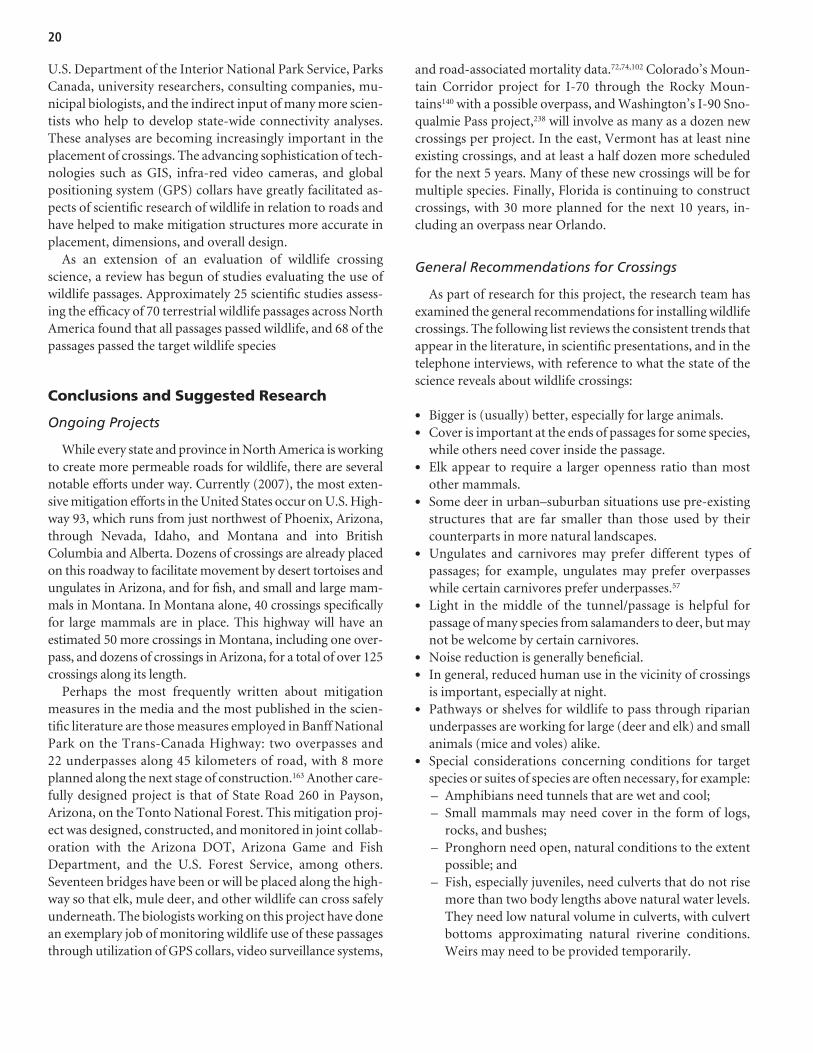
20

U.S. Department of the Interior National Park Service, ParksCanada, university researchers, consulting companies, mu-nicipal biologists, and the indirect input of many more scien-tists who help to develop state-wide connectivity analyses.These analyses are becoming increasingly important in theplacement of crossings. The advancing sophistication of tech-nologies such as GIS, infra-red video cameras, and globalpositioning system (GPS) collars have greatly facilitated as-pects of scientific research of wildlife in relation to roads andhave helped to make mitigation structures more accurate inplacement, dimensions, and overall design.

As an extension of an evaluation of wildlife crossingscience, a review has begun of studies evaluating the use ofwildlife passages. Approximately 25 scientific studies assess-ing the efficacy of 70 terrestrial wildlife passages across NorthAmerica found that all passages passed wildlife, and 68 of thepassages passed the target wildlife species

Conclusions and Suggested Research

Ongoing Projects

While every state and province in North America is workingto create more permeable roads for wildlife, there are severalnotable efforts under way. Currently (2007), the most exten-sive mitigation efforts in the United States occur on U.S. High-way 93, which runs from just northwest of Phoenix, Arizona,through Nevada, Idaho, and Montana and into BritishColumbia and Alberta. Dozens of crossings are already placedon this roadway to facilitate movement by desert tortoises andungulates in Arizona, and for fish, and small and large mam-mals in Montana. In Montana alone, 40 crossings specificallyfor large mammals are in place. This highway will have anestimated 50 more crossings in Montana, including one over-pass, and dozens of crossings in Arizona, for a total of over 125crossings along its length.

Perhaps the most frequently written about mitigationmeasures in the media and the most published in the scien-tific literature are those measures employed in Banff NationalPark on the Trans-Canada Highway: two overpasses and 22 underpasses along 45 kilometers of road, with 8 moreplanned along the next stage of construction.163 Another care-fully designed project is that of State Road 260 in Payson,Arizona, on the Tonto National Forest. This mitigation proj-ect was designed, constructed, and monitored in joint collab-oration with the Arizona DOT, Arizona Game and FishDepartment, and the U.S. Forest Service, among others.Seventeen bridges have been or will be placed along the high-way so that elk, mule deer, and other wildlife can cross safelyunderneath. The biologists working on this project have donean exemplary job of monitoring wildlife use of these passagesthrough utilization of GPS collars, video surveillance systems,

and road-associated mortality data.72,74,102 Colorado’s Moun-tain Corridor project for I-70 through the Rocky Moun-tains140 with a possible overpass, and Washington’s I-90 Sno-qualmie Pass project,238 will involve as many as a dozen newcrossings per project. In the east, Vermont has at least nineexisting crossings, and at least a half dozen more scheduledfor the next 5 years. Many of these new crossings will be formultiple species. Finally, Florida is continuing to constructcrossings, with 30 more planned for the next 10 years, in-cluding an overpass near Orlando.

General Recommendations for Crossings

As part of research for this project, the research team hasexamined the general recommendations for installing wildlifecrossings. The following list reviews the consistent trends thatappear in the literature, in scientific presentations, and in thetelephone interviews, with reference to what the state of thescience reveals about wildlife crossings:

• Bigger is (usually) better, especially for large animals.• Cover is important at the ends of passages for some species,

while others need cover inside the passage.• Elk appear to require a larger openness ratio than most

other mammals.• Some deer in urban–suburban situations use pre-existing

structures that are far smaller than those used by theircounterparts in more natural landscapes.

• Ungulates and carnivores may prefer different types ofpassages; for example, ungulates may prefer overpasseswhile certain carnivores prefer underpasses.57

• Light in the middle of the tunnel/passage is helpful forpassage of many species from salamanders to deer, but maynot be welcome by certain carnivores.

• Noise reduction is generally beneficial.• In general, reduced human use in the vicinity of crossings

is important, especially at night.• Pathways or shelves for wildlife to pass through riparian

underpasses are working for large (deer and elk) and smallanimals (mice and voles) alike.

• Special considerations concerning conditions for targetspecies or suites of species are often necessary, for example:– Amphibians need tunnels that are wet and cool;– Small mammals may need cover in the form of logs,

rocks, and bushes;– Pronghorn need open, natural conditions to the extent

possible; and– Fish, especially juveniles, need culverts that do not rise

more than two body lengths above natural water levels.They need low natural volume in culverts, with culvertbottoms approximating natural riverine conditions.Weirs may need to be provided temporarily.

21

• Accompanying mitigation such as fencing and escaperamps are needed if exclusion fences are installed.

• Protecting both sides of the passages for long-term conser-vation is cost effective.

• Passages need to be seen by wildlife as they approach.Passage placement in a straight line of sight works betterthan those placements below or above the approach levels.

• Local biologists need to be involved in all phases of theproject.

• Adaptive management works: monitor and improve futuredesigns based on monitoring results.

• Providing several different types of crossings or adaptingcrossing for suites of species by providing cover, shelves,small tubes, or a culvert within a culvert improves perme-ability.

• Maintenance of passages and accompanying mitigation,especially the bottom of passages in riparian areas andholes in fencing, improve effectiveness of crossings.

• Monitoring of passage use for at least 3 years after con-struction will be beneficial because wildlife often take atleast 2 years to adapt, especially if they use the area only forseasonal migration.

Wildlife crossings and road ecology have evolved dramati-cally in the 37 years since the first crossings were installed inColorado and New York. Consideration of wildlife and roadswill continue to require the attention of road engineers, trans-portation planners, and the public. In fact, a recent survey ofover 1,000 registered voters in the United States found that89% of those surveyed felt that roads and highways were athreat to wildlife.242 It is in the resource’s and the public’s bestinterest that road ecologists and engineers work to maintainhigh professional standards that promote functioning andeffective wildlife passages across North America. This workincludes developing the knowledge necessary for installingmitigation measures that create a more permeable landscapewhere many different species of a range of mobility and sizescan cross over and beneath transportation corridors in theirdaily and seasonal movements. The goal of greater permeabil-ity will take dedicated work on the part of engineers andecologists to include consideration of wildlife passages in theearliest of stages of long-range transportation programs. Con-sideration at the project level, and post-project for passagemaintenance during routine maintenance operations will con-tinue to be important, as will sound ecological research todocument if passages meet stated goals and objectives. Com-munication among those interested in passages, as well as thosenot typically involved in ecosystem concerns, such as planners,engineers, and administrators, will be effective if it is proactiveand collaborative. It takes the efforts of a community to openlines of communication. Citizens can be proud of the approx-imately 677 terrestrial and more than 10,000 aquatic passages

that have been placed in North America. As engineers and ecol-ogists plan for the future, they can learn from both thesuccesses and failures and can build on the current level ofawareness among the professions and the public to create acontinent-wide system of passages. It is a vision that will taketime and requires the collective efforts of all stakeholders.

2.3 Priorities in Research and Practice

Introduction

The field of transportation (road) ecology is developingswiftly and is practiced throughout North America and inter-nationally without a parent organization or society to helpguide research and practice. As a result, attempts to mitigatetransportation effects on wildlife can appear to be scattered andduplicative. National and continental efforts are under way todocument existing knowledge, accomplishments, and futureactions, and in particular how to mitigate the negative effectsof transportation corridors for wildlife.80,210,62,181 To determinefuture activities, a North American consensus regarding toppriorities for research and practice would prove most helpful.The research reported in this section is an effort to create a pri-oritized list of actions in safety and ecological research andpractices to help mitigate the negative impact of roads onwildlife in the United States and Canada. The objective was todetermine where additional research, field evaluations, andpolicy actions were needed in order to help maintain and re-store landscape connectivity and permeability for wildlifeacross transportation corridors, while also minimizing WVCs.

Research Approach: Methods and Data

Setting Priorities

The creation of the list of gaps and priorities in trans-portation research and practice with respect to wildlife beganwith a review of the pertinent literature. Approximately 120priorities were generated by the research team and then ini-tially ranked and combined to create 25 priorities. The initialpriorities were sent to 31 professionals in federal and stateagencies and academic institutions across North America forreview and editing. Thirteen reviews of the document werereceived and information and edits from these reviews wereincorporated into the priorities, along with comments fromthe NCHRP Project 25-27 panel.

Creating the Survey Instrument

During the development of an effective questionnaire, thepriorities were ranked and annotated by 27 attendees of the

22

Wildlife Crossings Workshop in Payson, Arizona, that wassponsored by the Southern Rockies Ecosystem Project, theArizona DOT, and the Arizona Game and Fish Department.These suggestions were incorporated into the survey instru-ment, and the survey was re-organized into a more conciseand easily understood document. For a second iteration, theupdated survey was presented to the attendees of the Deer-Vehicle Crash Workshop in Madison, Wisconsin. Eighteenparticipants submitted surveys with further suggestions forpriorities and improving the survey instrument. Their com-ments were incorporated into a final version that was pre-sented as an Internet survey. The survey instrument wasbased on Dillman’s70 methods for email surveys, and advicefrom R. Krannick (personal communication, Sociology De-partment, Utah State University, 2005). Participants wereasked to rank the priorities (with an option for “Not EnoughInformation”) on a scale of 0 (no priority) to 10 (top prior-ity) based on three criteria:

• Cost-effectiveness: Are the returns on the investment ofmoney for research and development worth the cost?

• Urgency: Does this priority need the most immediate ac-tion based on development pressures, safety issues, species’survival, transportation projects, and political climate?

• Overall effects: If this priority were accomplished, would ithave far-reaching results across geographic, political, dis-ciplinary, and ecological boundaries?

Although priorities were presented in two categories—practice (11 priorities listed) and science (14 priorities listed),participants were instructed to consider all priorities togetherwhen ranking. The priorities were placed into two categoriesto help direct management actions separately from researchactions. Each priority was ranked from 0 to 10, allowing formultiple identical values among a participant’s priorities.Five optional questions at the end of the survey pertained tothe participant’s job title, area of expertise related to trans-portation ecology, the state or province of employment, typeof employer, and email address. Participants submitted thesurvey by clicking on a “Submit Survey” button at the bottomof the page. They were given the option to print the surveyand to send it to others by e-mail.

Selection of Participants

The participants for the survey were selected using a non-random decision rule intended to select people with knowl-edge about transportation and wildlife issues in NorthAmerica. The largest set of potential survey respondentswas taken from the pool of participants in the telephonesurvey (Section 2.2) conducted as part of this NCHRPresearch project. Participants were targeted for their

knowledge of mitigation measures for wildlife and fish pop-ulations near roads, WVC data management and research,natural resource agency coordination, and transportationecology planning. Participants were research scientists, en-gineers, environmental and transportation planners, natu-ral resource managers, data managers, and administratorsworking for DOTs and MoTs, the FHWA, state wildlifeagencies, the U.S. Fish and Wildlife Service, the U.S. De-partment of the Interior Bureau of Land Management andNational Park Service, U.S. Forest Service, Parks Canada,and consulting companies. The pool also included aca-demic and federal research personnel involved in road ecol-ogy and road safety analyses. The pool of telephone surveyparticipants came from an original list of names taken fromprojects listed on the FHWA’s website “Keeping It Sim-ple,”85 the list of participants in the proceedings of the In-ternational Conference on Ecology and Transportation in 2001 and 2003,127,128 and recommendations from keyFHWA personnel involved in wildlife mitigation across thecountry. Canadian contacts were compiled by researchteam members and from lists of attendees of the TAC meet-ings. The goal of drawing from those resources was to makecontact with practitioners and researchers involved in roadecology as well as individuals from state DOTs and provin-cial MoTs who work with transportation and wildlife proj-ects. Those initial contacts led to many other contactsacross North America who potentially could contribute tothe telephone survey on wildlife and roads.66 The membersand friends of the Transportation Research Board’s TaskForce on Ecology and Transportation were also invited toparticipate in the survey. The initial 497 invited participantswere encouraged to pass the survey on to peers in theiragencies and professions who had knowledge that would as-sist them in ranking these priorities. This encouragementled to a snowball sample of a much larger population of un-known size.

Delivering the Survey

The potential survey participants were notified of the forth-coming survey during the last 3 days in March 2006. A secondemail was sent a week later with a request to take the surveyonline or to print the survey and send a hard copy to the re-search team. Potential participants were given 17 days to takethe survey before it was closed. Four days prior to the closingof the survey, all participants who had not taken the survey, orwho had taken the survey but did not give their email ad-dresses, were sent a final reminder. During the last 2 days ofthe survey, an additional 17 potential Canadian participantswere included in the survey mailings, and survey availabilitywas extended for 1 week. The survey was officially closed 28 days after it was opened.

23

Statistical Analysis

Survey results were analyzed using the SPSS software pro-gram.221 Analyses of variance (ANOVA) were conducted forcomparing mean values of each priority as rated by differentclasses of survey participants. The Levine statistic was first runto test for homogeneity of variance. When variances amongthe different mean values of a priority among the differentparticipants were not equal (as shown by a significant Levinestatistic), ANOVA was not used, and the Welch test, whichaccounts for unequal variances, was used to test for signifi-cant differences in priority means. F-tests were used in caseswhere means met the equal variances assumption of ANOVA.The Games–Howell post hoc test was used to determine thelocational significant differences between means as shown bythe ANOVAs and Welch tests. This particular post hoc test isdesigned to account for both unequal variances as well as un-equal sample sizes.

Findings and Results

Survey Participants

The original pool of 497 individuals was initially invited viaemail to participate in the survey. A total of 444 individualsparticipated. Of those 444, 388 participants (87.3%) chose toidentify themselves by submitting their email address. Ofthose 388 email addresses, 254 (65.5%) were identified asmembers of the original pool of invitees. Response rate of theoriginal invitees who gave their email addresses was 51.5%.The actual response rate is unknown because 56 participantsdid not submit their email addresses. One hundred andthirty-four (30.2%) of the email addresses given did notmatch the original pool of invited participants’ email ad-dresses. These participants were invited by others to take thesurvey and thus their participation created what is known asa snowball sample.

Participants represented all of the United States with theexception of Oklahoma, and the Canadian provinces and ter-ritories with the exceptions of New Brunswick, NorthwestTerritories, and Prince Edward Island. Of the 444 par-ticipants, 403 (90.8%) were from the United States and 36 (8.1%) were from Canada (Table 1). Five participants didnot indicate their state/province of employment. Participantswere asked to generalize the type of employer they workedfor. Table 2 lists the number of survey participants employedby each type of employer. The majority of respondents (n =183, 41.2%) were employed by a state/provincial transporta-tion agency. The second largest group of respondents werethose that worked for a federal natural resource agency (n =70, 15.8%). The remaining respondents worked forstate/provincial natural resource agencies (n = 55, 12.4%),universities (n = 45, 10.1%), consulting firms (n = 37, 8.3%),

federal transportation agencies (n = 25, 5.6%), non-profitgroups (n = 23, 5.8%), or other/unknown (n = 6, 1.3%). Eachperson was asked to list his/her job title and area of specialtyrelated to roads and wildlife. From these data, each partici-pant was classified into one of seven different profession types(Table 3): engineers/analysts/GIS specialists (n = 61, 13.7%),planners (n = 13, 2.9%), natural resources-manager (n = 38,8.6%), natural resources-non-profit (n = 23, 5.2%), naturalresources-planner (n = 187, 42.1%), natural resources-researcher (n = 109, 24.6%), unknown (n = 11, 2.5%) orother (n = 2, 0.5%). Natural resource professionals repre-sented 80.4% (357) of participants.

Ranking of Priorities

Priorities were ranked for overall value, and then withinthe practice or research categories by classification (nation oforigin, profession, and employer) of the participants. Therank of a priority was determined by adding all the scoressubmitted for that priority and calculating the mean value.For example, the top priority to incorporate wildlife mitiga-tion needs early in the planning processes received a total of441 rankings, ranging from 1 to 10. Those 441 values weresummed, and then the mean was calculated as 8.96, makingit the highest ranked priority. Tables 4 and 5 summarize theresults. The top five priorities are:

1. Incorporate wildlife mitigation needs early in theDOT/MoT programming, planning, and design process;

2. Better understand the dynamics of animal use of mitiga-tion structures (such as what works and what does not)and disseminate this information;

3. Combine several animal-friendly mitigation methodssuch as wildlife crossings, fences, escape ramps, and gates,rather than relying on just one method;

4. Use conservation plans and connectivity analyses to in-form the transportation programming/planning/designprocess on where mitigation is needed and how it may becarried out; and

5. Develop alternative cost-effective wildlife crossing designsand the principles upon which they are based.

Priorities by Nation

Practice priorities. The United States and Canadian partic-ipants ranked the first three priorities for practice identically:

1) Incorporate wildlife mitigation needs early in theDOT/MoT programming, planning, and design process;

2) Combine animal-friendly mitigation methods such aswildlife crossings, fences, escape ramps, and gates, ratherthan relying on using a single method; and

24

Employer Number of Participants Consulting 37 Federal Natural Resources 70 Federal Transportation 25 Non-profit 23 State/Provincial Natural Resources 55 State/Provincial Transportation 183 University 45 Unknown 5 Other 1 Total 444

Table 2. Number of survey participants employedby each type of employer.

State # Participants State # Participants United States

Alabama 3 Montana 24 Alaska 7 Nebraska 1 Arizona 33 Nevada 2 Arkansas 2 New Hampshire 5 California 73 New Jersey 2 Colorado 22 New Mexico 6 Connecticut 4 New York 9 Delaware 1 North Carolina 10 District of Columbia 8 North Dakota 2 Florida 7 Ohio 4 Georgia 10 Oklahoma 0 Hawaii 2 Oregon 15 Idaho 4 Pennsylvania 6 Illinois 2 Rhode Island 1 Indiana 1 South Carolina 8 Iowa 6 South Dakota 7 Kansas 5 Tennessee 3 Kentucky 4 Texas 14 Louisiana 2 Utah 16 Maine 3 Vermont 2 Maryland 3 Virginia 13 Massachusetts 4 Washington 3 Michigan 3 West Virginia 1 Minnesota 10 Wisconsin 2 Mississippi 1 Wyoming 22 Missouri 5 Unknown 5

Total # U.S. Participants = 408

Province # Participants Province # Participants Canada

Alberta 7 Ontario 7 British Columbia 10 Quebec 3 Manitoba 3 Saskatchewan 1

Yukon 3 Newfoundland and Labrador 1

Nova Scotia 1 Total # Canadian Participants = 36

Table 1. Number of survey respondents within each U.S. state and Canadian province.

Effective communication and collaboration among stake-holders was ranked fourth in the United States and fifth inCanada. The use of standard protocols for roadkill andanimal–vehicle collision data was ranked fourth in Canada.The incorporation of plans and schedules that can be accom-plished by maintenance crews was ranked fifth in the UnitedStates (See Appendix A, Table 37).

Research priorities. In ranking the research priorities,the two nations diverged to a greater degree than on rankingpractice priorities. Participants from both countries rankedthe need to better understand animal use of mitigation struc-tures as the top research priority. The development of cost-effective crossing designs was ranked second in the UnitedStates and third in Canada. Canadians ranked the need forstandardized data collection of roadkill carcasses and WVCsas their second research priority. In the United States, the third

3) Use conservation plans and connectivity analyses to in-form the transportation programming/planning/designprocess on where mitigation is needed and how it is to becarried out.

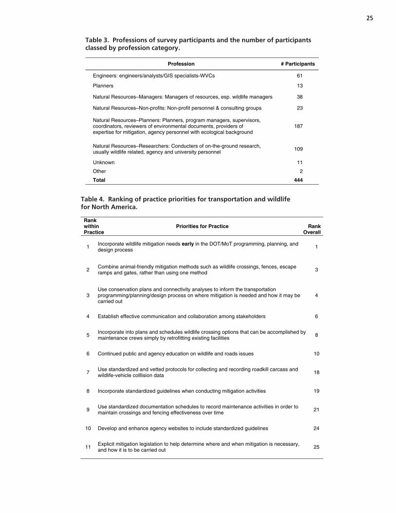
25

Profession # Participants

Engineers: engineers/analysts/GIS specialists-WVCs 61

Planners 13

Natural Resources–Managers: Managers of resources, esp. wildlife managers 38

Natural Resources–Non-profits: Non-profit personnel & consulting groups 23

Natural Resources–Planners: Planners, program managers, supervisors, coordinators, reviewers of environmental documents, providers of expertise for mitigation, agency personnel with ecological background

187

Natural Resources–Researchers: Conducters of on-the-ground research, usually wildlife related, agency and university personnel

109

Unknown 11

Other 2

Total 444

Table 3. Professions of survey participants and the number of participantsclassed by profession category.

Rankwithin Practice

Priorities for Practice Rank Overall

1 Incorporate wildlife mitigation needs early in the DOT/MoT programming, planning, and design process

1

2 Combine animal-friendly mitigation methods such as wildlife crossings, fences, escape ramps and gates, rather than using one method 3

3Use conservation plans and connectivity analyses to inform the transportation programming/planning/design process on where mitigation is needed and how it may be carried out

4

4 Establish effective communication and collaboration among stakeholders 6

5 Incorporate into plans and schedules wildlife crossing options that can be accomplished by maintenance crews simply by retrofitting existing facilities 8

6 Continued public and agency education on wildlife and roads issues 10

7 Use standardized and vetted protocols for collecting and recording roadkill carcass and wildlife-vehicle colllision data 18

8 Incorporate standardized guidelines when conducting mitigation activities 19

9 Use standardized documentation schedules to record maintenance activities in order to maintain crossings and fencing effectiveness over time 21

10 Develop and enhance agency websites to include standardized guidelines 24

11 Explicit mitigation legislation to help determine where and when mitigation is necessary, and how it is to be carried out 25

Table 4. Ranking of practice priorities for transportation and wildlife for North America.

26

Rankwithin Research

Priorities for Research Rank Overall

1 Understand better the dynamics of animal use of mitigation structures (such as what works and what does not) and disseminate this information

2

2 Develop and summarize alternative, cost-effective wildlife crossings designs and the principles they are based on 5

3 Develop wildlife crossing structure designs and guidelines for the full suite of animals in an area to help facilitate permeability for many species 7

4 Develop state-based habitat connectivity analyses for every state 9

5 Develop a standardized monitoring protocol to assess crossing effectiveness 11

6 Develop guidelines to decide when wildlife mitigation is necessary (both mandated and voluntary) 12

7 Develop standardized inventories of wildlife crossings by state for better management and maintenance of these crossings, and to better assess the need for future crossing 13

8 Increase our understanding of the effects of road density on wildlife populations 14

9 Develop prototype animal/vehicle collision safety models to predict where wildlife-vehicle colllision “hotspot” areas are and may be on future roads 15

10Improve ecosystem valuation for use in mitigation measures, to help establish mitigation cost-effectiveness (such as monetary value of the reduction of wildlife–vehicle collisions, or increased landscape permeability)

16

11 Standardize spatially accurate roadkill carcass and wildlife-vehicle colllision data collection 17

12Create a comprehensive synthesis document that establishes the indirect effects of roads and road density on ecosystems, and how these cumulative effects may in turn influence landscape permeability for wildlife

20

13 Develop reliable methods to estimate how often wildlife are in or near the road to help assess their potential in becoming involved in wildlife–vehicle collisions 22

14 Understand better the genetic consequences of the roaded landscape on animal populations 23

Table 5. Ranking of research priorities for transportation and wildlife in North America.

ranked research priority was the need to develop structure de-signs and guidelines to provide landscape permeability for thefull suite of animals in an area, and the fourth ranked prioritywas the need to develop state-based connectivity analyses. InCanada, the fourth ranked priority was the need to developguidelines for when wildlife mitigation was necessary. For thefifth research priority, U.S. citizens ranked the need to developprotocols for judging the effectiveness of wildlife crossing,while Canadians ranked the need for the development of pro-totype WVC models to predict priority hotspots (See Appen-dix A, Table 38).

Priorities by Profession

Practice priorities. Priorities were ranked among the threemajor classes of participants: engineers/analysts/GIS Specialists,natural resource professionals (all types combined), and plan-ners. Engineers, planners, and natural resource professionals allhad the same top five practice priorities, but ranked differentlyby profession. Different median values among the professionsare noted, with engineers generally rating each of the top fivepriorities a lower median value, and planners rating all five toppriorities relatively high median values. Incorporating wildlife

27

mitigation needs early in planning was ranked as the top prior-ity by all professions except by planners. The median rankedvalue for this priority among planners was 9.0, similar to the 9.1value for natural resource professionals. However, plannersrated the need to combine animal-friendly mitigation methodspriority as number one (9.2 median value), and early planningas their second highest priority. Engineers ranked the need foreffective communication second, while natural resourceprofessionals ranked the need to combine animal-friendly mit-igation methods second. Using conservation plans and connec-tivity analyses ranked alternatively third and fourth among allthree professions. Further ranking of the top five practice pri-orities for the three professions can be seen in Appendix A:Tables 39, 40, and 41.

Research priorities. All professions ranked the followingtop two priorities identically: to better understand the dy-namics of animal use of mitigation structures, and to developalternative, cost-effective crossing designs. Planners and nat-ural resource professionals ranked the need to developwildlife crossing structure designs and guidelines for the fullsuite of animals in an area third, while engineers/analystsranked it fifth, and the need to develop guidelines to decidewhen wildlife mitigation is necessary as third. The fourth andfifth ranked research priorities among the different profes-sions were not as closely ranked as the top five practice prior-ities (Appendix A: Tables 39, 40, and 41), and select prioritieswere ranked significantly different.

Priorities by Employer

Practice priorities. The top five practice priorities for allemployer classes were identical but ordered differently. Thetop priority of the survey, early planning for wildlife, was ratednumber one by all except federal transportation professionals(ranked third) and consulting company personnel (rankedsecond). The second ranked practice priority, to combineanimal-friendly mitigation methods, was ranked differentlyamong the different types of employees. The third practice pri-ority, to use conservation plans and connectivity analyses, wasrated as the top priority by federal transportation agency em-ployees, second by federal and state natural resource agencypersonnel, and those working for non-profit groups, and thirdor fourth for the remaining types of employees. The fourthpractice priority, to establish effective communication, wasranked as the second highest priority by those working for fed-eral and state transportation agencies, and fourth or fifth for allother types of employees. The fifth overall practice priority, toincorporate wildlife crossing options that can be accomplishedby maintenance crews through retrofits, was ranked eitherfourth or fifth among all types of employees. Further detail isprovided in Appendix A (Tables 39, 40, and 41).

Research priorities. The top five research priorities werenot as tightly ranked as the practice priorities among em-ployer classes. The top four research priorities were eachwithin the top six rankings of every employee class; however,each class ranked them differently. For example, the overallnumber one priority to better understand the dynamics ofanimal use of mitigation structures was ranked by every classof employee as number one, except for consulting companypersonnel who ranked this priority second and the need forcost-effective crossing designs as their number one priority.Several priorities were ranked within the top five of specificemployee groups but did not make the top five overallresearch priorities. University professionals (typically re-searchers) ranked fourth the need to develop guidelines todecide when wildlife mitigation is necessary, as did those em-ployed by state/provincial transportation agencies and thoseworking for consulting companies. This priority was ratedsixth for research in the overall survey. University profes-sionals and natural resource agency professionals rated theneed to increase our understanding of the effects of road den-sity on wildlife populations fifth and fourth, respectively,while it rated eighth overall.

The priority to improve ecosystem valuation for use inmitigation measures and to help establish cost-effectivenesswas rated overall as the tenth research priority, but was highlyrated by two types of employees, those working for non-profitorganizations (rated second), and federal transportationagency professionals (rated fifth).

Interpretation, Appraisal, and Applications

There was a consistent trend in the results for participants,regardless of geography, profession, or employer type, to rankthe same five practice priorities in their top five. The oneexception was the fourth rank that 36 Canadians gave to theneed for the use of standardized and vetted protocols for col-lecting and recording roadkill carcass and WVC data. OtherCanadian differences may be in part because the majority ofCanada still has its full suite of large animals. With such adiversity of wildlife, the risks to drivers from collisions withboth ungulates and predators are much greater than typicalanimal collisions in the United States. However, because of thelow number of Canadian participants, the research team can-not extrapolate the importance of this priority to Canada, butit represents a trend worth mentioning.

These results provide clear guidance to help governments,agencies, organizations, universities, companies, and indi-viduals focus their efforts in developing the future state ofpractice. Fundamental parameters will include early incor-poration of wildlife needs into the planning processes, a com-bination of animal-friendly mitigation methods rather thanjust fences, conservation plans and connectivity analyses to

28

inform transportation planning and design processes, effec-tive communication among stakeholders, and incorporationof plans and schedules for wildlife crossing options that canbe accomplished by maintenance crews by simple retrofit ofexisting facilities.

In ranking the research priorities, the different classes ofparticipants exhibited more widely varied values than in theirranking of practice priorities. The top ranked research prior-ity, to better understand the dynamics of animal use of mitiga-tion structures, was the top research priority for all categoriesof nation of origin, profession, and employers except forthose working for consulting firms who ranked it second. Thesecond overall research priority, to develop cost effectivewildlife crossing designs, ranked first among those working forconsulting companies, and third among Canadians, state andfederal natural resource agency personnel, and universitypersonnel. Those working for non-profit organizations gaveit a lower value of sixth. The third research priority, to developwildlife crossing structure designs and guidelines for the full suiteof animals, received a variety of rankings from the differentcategories of participants, but was consistently in the top fivepriorities for all categories of participants. The fourth overallresearch priority, to develop state-based habitat connectivityanalyses, was ranked within the top six priorities by all classi-fications of participants, except by those from Canada(eleventh), engineers (tenth), and planners (eighth). The fifthresearch priority, to develop a standardized monitoring proto-col to assess crossing effectiveness, was ranked within the top sixpriorities by residents of both the United States and Canada,all professions, and all employees of state and federal agen-cies. Every one of the top five research priorities was a top-fiveresearch priority for all the professions with the exception ofthe need to develop state-based habitat connectivity analyses,which planners and engineers did not value as highly as nat-ural resource professionals.

The results of the ranking of research priorities show theoverall high support for the top three: to better understandthe dynamics of animal use of mitigation structures, to de-velop cost-effective wildlife crossings designs, and to developwildlife crossing structure designs and guidelines for the fullsuite of animals. These and other research priorities can helpform a clearer picture of the areas in need of highest researchattention. They also demonstrate a need to better communi-cate the results of these research efforts.

Statistical differences among professions’ median rankingof priorities were significant for select priorities, but may bedue in part to the tendency of engineers to systematically uselower values for overall ranking while other professionssystematically use higher numbers to rank priorities.

Priority rankings were also heavily influenced by the dis-crepancy in number of participants from certain classes.Although efforts were made to include as many engineers

and Canadians as possible, their numbers remained lowerthan natural resource professionals and Americans, respec-tively. The rankings were also influenced heavily by the highnumbers of transportation professionals working for stateDOTs and provincial MoTs. This is in direct accordancewith the job responsibilities of this class, and they are themost appropriate employees for this continental survey.This class had the most representation in the survey (n =181), and as such, this employee class was the most influen-tial in ranking priorities. For example in the research prior-ities, the need for alternative cost-effective designs wasranked as first or second by only three employee classes,yet it was rated overall as the second research priority, inpart because of the large number of participants in thestate/provincial and federal employee categories who over-all rated it as the second highest research priority. The dif-ferences among different classes of respondents were in partaccounted for when priority rankings were separated by na-tion, profession, and employer, so readers could view thepriorities from these different perspectives.

Conclusions and Suggested Research

The research team identified the top 25 priorities forresearch and practice in the field of transportation and wildlifefor North America. The results show a clear consensus amongall participants on the top five practice priorities:

1. Incorporate wildlife mitigation needs early in the DOT/MoT programming, planning, and design process;

2. Combine several animal-friendly mitigation methodssuch as wildlife crossings, fences, escape ramps, and gates,rather than relying on just one method;

3. Use conservation plans and connectivity analyses toinform the transportation programming/planning/designprocess on where mitigation is needed and how it may becarried out;

4. Establish effective communication and collaborationamong stakeholders; and

5. Incorporate wildlife crossing options into plans andschedules that can be accomplished by maintenance crewsby simple retrofit of existing facilities.

These statements call for a plan of action. In Appendix A, thebackground and the next steps for these and all priorities aredescribed.

Priorities for research presented a greater challenge for con-sensus of opinion and were not as consistently rated by surveyparticipants. In general, the top three research priorities wereamong the top five research priorities by all categories of par-ticipants. The top three most consistently highly rated researchpriorities for North America are:

29

1. To better understand the dynamics of animal use of miti-gation structures (such as what works and what does not)and disseminate this information;

2. To develop and summarize cost-effective wildlife crossingdesigns and the principles they are based on; and

3. To develop wildlife crossing structure designs and guide-lines for the full suite of animals in an area to help facilitatepermeability for many species.

These priority statements lead to the next step, which is todescribe what is known, and how that knowledge can be builtupon. The intent of this research is to help inform mitigative ac-tions across North America that create a roaded landscape thatis more permeable for wildlife and safer for motorists. For

example, the top five priorities can lead agency personnel indirecting early planning for wildlife in transportation planning,help encourage the installation of suites of mitigation measuresfor wildlife, promote the use of connectivity analyses in trans-portation planning, and the development and use of alternativecost-effective crossing designs. Researchers can see the need todesign studies that address our need to better understand the dy-namics of animal use of mitigation structures, and disseminatethis information. Additional priorities can help raise awarenessfor the need for better communication among agency person-nel and the public, and help states to initiate standardized guide-lines and methodologies involved in wildlife crossings andWVCs. Organizations working at the national level may usethese guidelines to help direct policy initiatives as well.

30

3.1 Safety Data Analysis Aspects

Introduction

This research segment covers the work done for the safetydata analysis aspects of the project. Throughout this reportthe words “collision” and “crash” are used interchangeably.

The broad objectives of this project required an analysis ofWVCs and road environment data from state DOT sources.Specifically, the planned purpose of the safety analysis was toproduce results that would assist with the development ofguidelines on:

• Methods for identifying WVC problem locations,• The evaluation of the safety effectiveness of crossing miti-

gation measures,• The establishment of a monitoring program to facilitate the

identification of collision-prone locations and the evaluationof crossing mitigation measures, and

• Cost-benefit and cost-effectiveness considerations.

The following sections document efforts towards developingthese guidelines. The two aspects to the safety research,although linked, are summarized separately:

• Aspect 1: The application of reported WVC data typicallyavailable in state DOT databases and

• Aspect 2: An investigation of how the application of twodatabases, reported WVCs and carcass removals, can leadto different roadway improvement decisions

Aspect 1: Application of Reported Wildlife–VehicleCollision Data

The general objectives of the research undertaken for thisaspect are consistent with those of SafetyAnalyst (www.safetyanalyst.org), a safety management guide being devel-oped by the FHWA for use by DOTs. SafetyAnalyst is

envisioned as a set of software guides used by state and localhighway agencies for safety management and to improvetheir programming of site-specific safety improvements.SafetyAnalyst incorporates state-of-the-art safety manage-ment approaches into computer-based analytical guides to aidthe decision-making process to identify safety improvementneeds and develop a systemwide program of site-specificimprovement projects. The general objectives of this researchaddress three general aims:

1. Identify collision-prone locations for existing or proposedroads for all collision types combined or for specific targetcollision types;

2. Aid in the evaluation, selection, and prioritization ofpotential mitigation measures; and

3. Evaluate the effectiveness of mitigation measures alreadyimplemented.

Meeting these objectives requires the use of state-of-the-artstatistical methods (e.g., predictive negative binomial modelsand empirical Bayes procedures) to produce a widely acceptedand usable guide that can be readily applied by DOTs in theircompletion of items 1 and 2 for animal–vehicle collisions andto provide initial insights as part of a framework for futureresearch to make additional progress on item 3 with respect towildlife crossings. It is expected that results of this researchproject, specifically the predictive models developed, can beapplied within SafetyAnalyst in undertaking tasks 1, 2, and 3above with respect to wildlife–vehicle collisions.

Aspect 2: Comparison of Wildlife–Vehicle Collisionand Carcass Removal Data

Reported WVC data may represent only a small portion ofthe large number of WVCs that occur61,201. A second type ofdata, obtained from records of carcass removals, has also beenused to describe the WVC problem and determine the need

C H A P T E R 3

Phase 2 Segments

31

for and impacts of WVC countermeasures. This aspect ofNCHRP 25-27 was conducted to investigate the hypothesisthat roadside carcass removal data not only indicate a differentmagnitude for the WVC problem, but may also show differ-ent spatial patterns than reported WVC data. The choice ofthe database (collisions or carcasses) used to evaluate theWVC problem, therefore, may lead to the identification ofdifferent hotspot locations and ultimately different counter-measure improvements. Patterns were examined visually byGIS plots, and by the development of comparable negativebinomial WVC and deer carcass removal models. WVC anddeer carcass removal data were obtained from the IowaDepartment of Transportation (IaDOT).

The creation and analysis of GIS-based data that include theattributes and location of roadway segment cross sections,reported WVCs, and deer carcass removals can be used to an-swer a number of questions:

• Is the number of reported deer carcass removals differentthan the reported number of WVCs statewide and alongindividual roadway segments?

• Are different “high collision” segments identified whenreported WVCs and deer carcass removal data are used forthe safety analysis of individual roadway segments? Inother words, do they have different occurrence patterns?

• Are there any apparent relationships between traffic flow,roadway cross section characteristics, and reported WVCs?Are these relationships, if they exist, similar for deer carcassremoval data?

The activities completed as part of this aspect of NCHRP 25-27 (e.g., plots, summary measures, and models) were used toinvestigate and compare the patterns of two databases (i.e.,reported WVCs and deer carcass removals) that have beenused to define and mitigate the WVC problem.

Research Approach: Methods and Data

The research approach emerged from a review of the exist-ing literature, specifically from a consideration of the gaps inexisting knowledge.

Methods

Aspect 1: Application of reported wildlife–vehicle colli-sion data. Predictive models for wildlife–vehicle collisions(commonly called “safety performance functions” [SPFs])are crucial to state-of-the-art methods for filling safety analy-sis gaps and developing the requisite guidelines for mitigat-ing these collisions. These models are derived from historicaldata and relate collision frequency to physical roadway androadside characteristics and to measures of exposure. They

were developed for, and apply to, reported large-animalWVCs (as distinguished from data reported only as carcassremoval) and, with a view to the application of the models,for use only with those variables for which data are readilyavailable within the typical DOT safety databases. Becauseanimal exposure data (a measure of the numbers of animalsinvolved in WVC that are near the road, and the amount oftime they spend near the road over the course of a specificmeasured time unit) are not among these readily availablevariables, this approach will result in some unexplainedvariation in the dependent variable. The safety model inputsare limited to roadway (between shoulder edges) variablesbecause few DOT databases include roadside information(e.g., guardrail, roadside sight distance) or adjacent landscape(off right-of-way) characteristics. Even so, it is still necessaryto estimate models for lower levels of data availability thatmay exist in some jurisdictions. The result is three funda-mental levels of SPFs:

• Level 1: These SPFs include only the length and annualaverage daily traffic volume (AADT) of a segment.

• Level 2: These SPFs require that segments be classified asflat, rolling, or mountainous terrain and also use the lengthand AADT of a segment.

• Level 3: These SPFs include additional roadway variablessuch as average lane width in addition to the Level 2 variables.

The SPFs can be used in a number of applications:

• Application A: SPFs can be used with caution to identifyroadway factors associated with a high propensity forwildlife–vehicle collisions. These cautions pertain to possiblycounterintuitive inferences that may result from omitted, in-correctly specified, or correlated factors. This application canbe useful in roadway design and planning decisions that haveimplications for wildlife–vehicle collisions.

• Application B: SPFs can be used in the identification ofroadway segments that may be good candidates for wildlife–vehicle collision countermeasures.

• Application C: SPFs can be used in estimating the effec-tiveness of potential countermeasures that are consideredfor candidate segments.

• Application D: SPFs can be used in evaluating the effective-ness of implemented countermeasures using state-of-the-artmethods for observational before-after studies.114

For the last three applications, which are key elements inthis project, collision history often is used as a predictor.However, it is now well recognized as a poor predictor be-cause collision history tends to be short term (<3 years) ratherthan long term (≥3 years) and therefore subject to randomfluctuation and associated vagaries of regression to the mean.

32

The result is that for Application A, resources are oftenwasted on safer sites that are wrongly identified and goodcandidates may be ignored. As a result, the countermeasureeffectiveness estimates for Applications C and D can be exag-gerated. The regression to the mean problem cannot beoveremphasized and so is illustrated in Appendix D.

While the SPF can provide less biased predictions than thecollision count for Applications B, C, and D, estimates ob-tained from these models can have a high variance because ofthe inability to include potentially important explanatoryvariables in them. In recognition of this difficulty and theproblems with estimates from collision counts, an empiricalBayes (EB) procedure has been used.177 This procedure inessence takes a weighted average of the two estimates, recog-nizing that both provide important clues as to a location’ssafety. In effect, by using the collision counts to refine the SPFprediction, the EB procedure accounts for factors, such as offright-of-way characteristics and animal exposure, that affectwildlife–vehicle collision frequency but are not in the model.For example, a location that has more animal movementsthan the “average” location, but that is similar in the charac-teristics of the prediction model, will tend to have more col-lisions than the “average” location. With EB refinementcomes higher collision prediction accuracy. The EB proce-dure is illustrated by way of example applications, in the “In-terpretation, Appraisals, and Applications” section.

The development of the SPFs involved determination ofwhich explanatory variables should be used, if and how vari-ables should be grouped, and how variables should enter intothe model (i.e., the best model form). Consistent with the com-mon research practice in developing these models, generalizedlinear modeling was used to estimate model coefficients,assuming a negative binomial error distribution. In specifyinga negative binomial error structure, the dispersion parameterk, which relates the mean and variance of the regression esti-mate, is estimated from the model and the data. The value ofk is such that, the smaller its value, the better a model is for theset of data (See Appendix B). Conveniently, the dispersionparameter estimated in the SPF calibration is used to derivethe weights for the two sets of information used in the EBprocedure.

Aspect 2: Comparison of wildlife–vehicle collision andcarcass removal data. The tasks completed for this researchwere done to evaluate the value of collecting and plottingWVC and deer carcass removal data by location, and to testthe straw hypothesis that these two datasets may also identifydifferent roadway locations for potential WVC countermea-sures. The magnitude and patterns of location-based WVCreports and deer carcass removal datasets in Iowa were com-pared qualitatively through visual GIS plots and quantita-tively (e.g., WVC frequency per mile). The GIS plots and

summary tables from these comparison activities are sum-marized in the “Findings and Results” section. Similar to As-pect 1, negative binomial prediction models were also used.WVC and deer carcass removal prediction models (or SPFs)that considered traffic flow and roadway cross section ele-ments as potential input variables were created and com-pared. The results of these activities are also described in the“Findings and Results” section.

Several types of computer software were used to overlay,present, and summarize the WVC and deer carcass removaldata within the GIS platform. Microsoft® Excel™ and True-Basic™ were used to manage the deer carcass removal data.The ArcGIS 9.1™ platform was used to present and analyzethe collision and carcass datasets spatially. ArcCatalog™ wasused as a file management program and applied specificallyfor organizing spatial data. Most of the mapping activitiestook place in ArcMap™. ArcGuidebox™ was used for someof the more complicated spatial analysis, and the large size ofthe roadway inventory database files required the use ofFileMaker™. The modeling of the WVC and deer carcassremoval information was completed with SAS™ statisticalsoftware.

Data

Aspect 1: Application of reported wildlife–vehicle collisiondata. The models for predicting the frequency of reportedwildlife–vehicle collisions were developed for rural two-laneand rural multilane roadways using Highway Safety Informa-tion System (HSIS) data from California, North Carolina,Utah, and Washington and for rural freeway roadways withdata from California, Utah, and Washington. These are thetypical classifications used by DOTs in other aspects of safetymanagement. Tables 6 through 9 summarize the data used.

Aspect 2: Comparison of wildlife–vehicle collision andcarcass removal data. Three different databases were usedto compare the magnitude and patterns of WVCs and deercarcass removals in Iowa. First, 10 years of police-reportedWVC information in a GIS-acceptable format were acquiredfrom the IaDOT. The data included the location of the WVCsand information provided on the police reports (e.g., sever-ity, surface conditions, time of day, and age of driver). A largemajority of the reported WVCs involved white-tailed deer(Odocoileus virginianus). The reported WVCs in 2001, 2002,and 2003 were used in this analysis. The individual WVClocations were provided by the IaDOT and plotted by latitudeand longitude coordinates. For example, the 2002 WVClocations plotted on a roadway map of Iowa within a GISplatform are shown in Figure 4.

The two other datasets that were used included informa-tion about deer carcass removals and roadway cross sections.

33

Length (mi.) AADT Crashes/mile-year State Dataperiod Total mean min max mean min max

TotalCrashes mean min max

CA 1991-2002 8,349 0.644 0.001 26.137 4893 63 37041 5,378 0.068 0.000 16.670

NC 1990-2001 25,165 1.322 0.010 18.980 2466 2 80428 59,280 0.140 0.000 8.330

UT 1985-2000 9,260 2.503 0.010 40.380 1541 1 17424 15,334 0.186 0.000 6.250

WA 1993-1996 5,362 0.601 0.010 28.660 4334 87 23917 1,746 0.078 0.000 12.500

Table 6. Data summary for rural two-lane roadways.

Length (mi.) AADT Crashes/mile-year State DataPeriod Total Mean min max mean min max

TotalCrashes mean min max

CA 1991-2002 994 0.359 0.003 7.689 14312 304 78300 1,205 0.116 0.000 4.900

NC 1990-2001 1,185 0.803 0.010 9.440 11134 100 63332 5,406 0.347 0.000 8.330

UT 1985-2000 291 0.599 0.010 4.840 6162 186 61393 4,021 0.654 0.000 6.430

WA 1993-1996 322 0.423 0.010 63.440 12588 172 54274 251 0.218 0.000 12.500

Table 7. Data summary for rural multilane roadways.

Length (mi.) AADT Crashes/mile-year State Years of Data Total Mean min max Mean Min max

TotalCrashes mean min max

CA 1991-2002 1,659 0.536 0.001 14.917 22520 3275 86700 1,326 0.089 0.000 9.260

UT 1985-2000 700 1.928 0.010 13.730 10579 2776 64402 5,145 0.608 0.000 7.290

WA 1993-1996 400 0.685 0.010 8.320 18179 4124 49952 257 0.194 0.000 25.000

Table 8. Data summary for rural freeways.

State Roadway Variables State Roadway Variables

CA

AADTDesign speed in mph Divided/undividedLane width in feet Shoulder width in feet Median barrier type Median width in feet Number of lanes Surface type Surface width in feet Terrain (level, rolling, mountainous)

UT

AADTAverage degree of curvature Design speed in mph Lane width in feet Median type Median width in feet Number of lanes Paved roadway width in feet Percentage truck traffic Shoulder type Speed limit in mph Terrain (level, rolling, mountainous)

NC

AADTShoulder type Shoulder width in feet Median type Median width in feet Number of lanes Speed limit in mph Surface width in feet Terrain (level, rolling, mountainous)

WA

AADTAverage degree of curvature Shoulder width in feet Shoulder type Median barrier type Median width in feet Median type Number of lanes Speed limit in mph Surface width in feet Terrain (level, rolling, mountainous)

Table 9. Variables available for modeling.

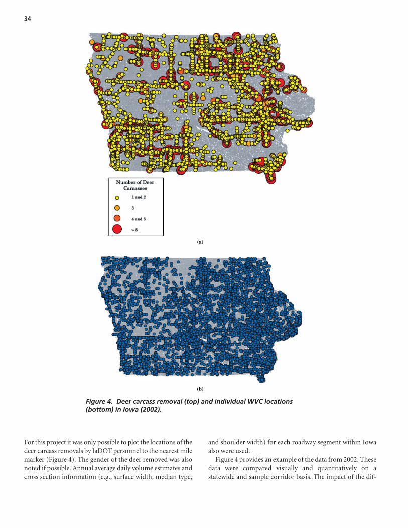
34

(a)

(b)

Figure 4. Deer carcass removal (top) and individual WVC locations (bottom) in Iowa (2002).

For this project it was only possible to plot the locations of thedeer carcass removals by IaDOT personnel to the nearest milemarker (Figure 4). The gender of the deer removed was alsonoted if possible. Annual average daily volume estimates andcross section information (e.g., surface width, median type,

and shoulder width) for each roadway segment within Iowaalso were used.

Figure 4 provides an example of the data from 2002. Thesedata were compared visually and quantitatively on astatewide and sample corridor basis. The impact of the dif-

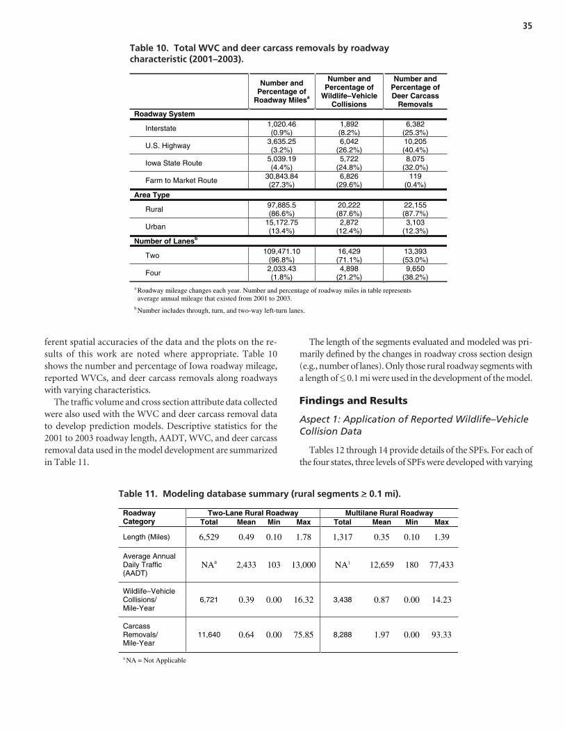
35

Number and Percentage of

Roadway Milesa

Number and Percentage of

Wildlife–VehicleCollisions

Number and Percentage of Deer Carcass

Removals Roadway System

Interstate 1,020.46(0.9%)

1,892(8.2%)

6,382(25.3%)

U.S. Highway 3,635.25(3.2%)

6,042(26.2%)

10,205(40.4%)

Iowa State Route 5,039.19(4.4%)

5,722(24.8%)

8,075(32.0%)

Farm to Market Route 30,843.84(27.3%)

6,826(29.6%)

119(0.4%)

Area Type

Rural 97,885.5(86.6%)

20,222(87.6%)

22,155(87.7%)

Urban 15,172.75(13.4%)

2,872(12.4%)

3,103(12.3%)

Number of Lanesb

Two 109,471.10(96.8%)

16,429(71.1%)

13,393(53.0%)

Four 2,033.43(1.8%)

4,898(21.2%)

9,650(38.2%)

a Roadway mileage changes each year. Number and percentage of roadway miles in table represents average annual mileage that existed from 2001 to 2003.

b Number includes through, turn, and two-way left-turn lanes.

Table 10. Total WVC and deer carcass removals by roadway characteristic (2001–2003).

ferent spatial accuracies of the data and the plots on the re-sults of this work are noted where appropriate. Table 10shows the number and percentage of Iowa roadway mileage,reported WVCs, and deer carcass removals along roadwayswith varying characteristics.

The traffic volume and cross section attribute data collectedwere also used with the WVC and deer carcass removal datato develop prediction models. Descriptive statistics for the2001 to 2003 roadway length, AADT, WVC, and deer carcassremoval data used in the model development are summarizedin Table 11.

The length of the segments evaluated and modeled was pri-marily defined by the changes in roadway cross section design(e.g., number of lanes). Only those rural roadway segments witha length of <_ 0.1 mi were used in the development of the model.

Findings and Results

Aspect 1: Application of Reported Wildlife–VehicleCollision Data

Tables 12 through 14 provide details of the SPFs. For each ofthe four states, three levels of SPFs were developed with varying

Two-Lane Rural Roadway Multilane Rural Roadway Roadway Category Total Mean Min Max Total Mean Min Max

Length (Miles) 6,529 0.49 0.10 1.78 1,317 0.35 0.10 1.39

Average Annual Daily Traffic (AADT)

NAa 2,433 103 13,000 NA1 12,659 180 77,433

Wildlife–VehicleCollisions/Mile-Year

6,721 0.39 0.00 16.32 3,438 0.87 0.00 14.23

CarcassRemovals/ Mile-Year

11,640 0.64 0.00 75.85 8,288 1.97 0.00 93.33

a NA = Not Applicable

Table 11. Modeling database summary (rural segments > 0.1 mi).

36

Model Form: Total wildlife–vehicle collisions/mile-year

= LANEWIDSPEEDHISURFWIDAADT 5432exp1

State/Model Terrain

ln(s.e.)

1

(s.e.)2

(s.e.)3

(s.e.)4

(s.e.)5

(s.e.)Dispersionparameter

CA 1 All -7.8290(0.1868)

0.6123(0.225) 1.6098

Flat -8.7034(0.2005)

Rolling -8.1810(0.1930)

CA 2

Mountainous -8.0343(0.1989)

0.6636(0.0228) 1.4831

Flat -8.5357(0.2046)

Rolling -7.9275(0.1968)

CA 3

Mountainous -7.7157(0.2029)

0.6518(0.0230)

Design55

-0.3310(0.0449) Else = 0

1.4493

NC 1 All -4.5625(0.0576)

0.3743(0.0078)

0.9222

FlatRolling

-4.3984(0.0745)

NC 2 Mountainous -5.5363

(0.0653)

0.3637(0.0077)

0.8142

FlatRolling

-4.3805(0.0773)

NC 3 Mountainous -5.7195

(0.0685)

0.4447(0.0087)

-0.0122(0.0022)

Posted< 55

-0.7165(0.0248) Else = 0

0.7353

UT 1 All -9.1135(0.1423)

1.0237(0.0205) 1.7610

Flat -9.3123(0.3385)

Rolling -9.0528(0.3393)

UT 2

Mountainous -8.7728(0.3006)

1.0092(0.0410) 1.6123

Flat -12.987(0.9608)

Rolling -12.803(0.9613)

UT 3

Mountainous -12.408(0.9485)

0.8073(0.0455)

Posted 55

-0.6646(0.1344) Else = 0

0.4751(0.0838)

1.3985

WA 1 All -8.6850(0.3020)

0.7802(0.0367)

1.3825

WA 2 All -8.5319(0.3552)

0.8034(0.0426)

-0.0584(0.0117) 1.0237

WA 3 All -8.5161(0.3493)

0.7622(0.0426)

-0.0696(0.0124)

Posted55

0.4358(0.0964) Else = 0

0.9528

Table 12. SPFs for rural two-lane roadways.

data requirements. The first level required only the length andAADT of a segment. The second level included the requirementthat segments be classified as flat, rolling, or mountainous ter-rain. The third level of SPFs added additional roadway variablessuch as average lane width. All variables were from state HSISdata. Segments were defined as sections of roads, generally be-tween significant intersections and having essentially commongeometric characteristics. Illustration of the application of theSPFs developed is a key component of this aspect of the safety

research. These applications are illustrated in the “Interpreta-tion, Appraisals, and Applications” section.

In general, the calibrated SPFs make good intuitive sense inthat the sign, and to some extent the magnitude, of the esti-mated coefficients and exponents accord with expectations.Surprisingly, the exponent of the AADT term, although rea-sonably consistent for the three levels of models in a state, variedconsiderably across states. This exponent varied significantlyacross facility types, reflecting differences in traffic operating

37

Model Form: Total wildlife–vehicle collisions/mile-year

= SPEEDHIMEDWIDAADT 432exp1

State/Model Terrain ln(s.e.)

1

(s.e.)2

(s.e.)3

(s.e.)

CA 1 All -5.2576(0.4397)

0.3290(0.0470)

Flat-6.4592(0.4523)

Rolling-5.7615(0.4398)

CA 2

Mountainous -5.5220(0.4498)

0.3926(0.0464)

Flat-6.4885(0.4485)

Rolling-5.8372(0.4360)

CA 3

Mountainous -5.6577(0.4462)

0.4145(0.0464)

-0.0057(0.0015)

NC 1 All -3.3660(0.6314)

0.2501(0.0684)

FlatRolling

-2.5310(0.6063)

NC 2 Mountainous

-4.1844(0.5934)

0.1736(0.0641)

FlatRolling

-2.4303(0.5871)

NC 3 Mountainous

-4.0785(0.5741)

0.1858(0.0621)

UT 1 All -4.1217(0.6231)

0.4414(0.0742)

Flat-4.4878(1.5295)

RollingUT 2

Mountainous -3.4508(1.5013)

0.3900(0.1754)

WA 1 All -12.7417(1.9219)

1.2066(0.2028)

Flat-12.9945(1.9091)

RollingWA 2

Mountainous -11.8326(1.8894)

1.1398(0.1987)

Flat-14.1608(2.1029)

RollingWA 3

Mountainous -13.2591(2.0800)

1.2721(0.2153)

0.1244(0.0775)

Table 13. SPFs for rural multilane roadways.

conditions. The variables found to be significant at the 10%level varied by state were:

AADT: Annual average daily trafficSURFWID: Total surface width (feet)LANEWID: Average lane width (feet)HI: Average degree of curvatureSPEED: Posted speed in North Carolina &

design speed in California (mph)MEDWID: Median width (feet)MEDTYPE: Positive barrier or unprotected

For application in another state, or even for applicationin the same four states for different years from those in thecalibration data, the models should be recalibrated to re-flect differences across time and space in factors such ascollision reporting practices, weather, driver demograph-ics, and wildlife movements. In essence, recalibrationinvolves using a multiplier, which is estimated to reflectthese differences by first using the models to predict thenumber of collisions for a sample of sites for the new stateor time period. The sum of the collisions for those sites isdivided by the sum of the model predictions to derive the

38

Model Form: Total wildlife–vehicle collisions/mile-year

= MEDTYPESURFWIDHIMEDWIDAADT 5432exp1

State/Model Terrain ln(s.e.)

1

(s.e.)2

(s.e.)3

(s.e.)4

(s.e.)5

(s.e.)Dispersionparameter

Flat -6.2814(0.7166)

RollingCA 1

Mountainous -4.7526(0.7098)

0.2810(0.0726)

1.5885

Flat -5.6746(0.6925)

RollingCA 2

Mountainous -4.3198(0.6857)

0.3050(0.0700)

-0.0126(0.0014) 1.3543

UT 1 All -4.3930(1.4121)

0.4356(0.1550)

1.9966

Flat -7.8707(1.4831)

Rolling -6.9760(1.4811)

UT 2

Mountainous -6.0374(1.4516)

0.7272(0.1632)

1.5641

Flat 8.0592(1.4808)

Rolling -7.1234(1.4773)

UT 3

Mountainous -6.0651(1.4465)

0.7472(0.1630)

MedianType

Positive barrier-1.0633(0.4623)

Unprotected 0.0000

1.5277

WA 1 All -15.5153(1.7866)

1.3969(0.1809) 0.8816

Flat -16.8612(1.7977)

Rolling -15.8572(1.7634)

WA 2

Mountainous -15.4443(1.7846)

1.4355(0.1784) 0.7807

Flat -9.9014(3.9034)

Rolling -8.8909(3.8877)

WA 3

Mountainous -8.4610(3.8975)

1.4507(0.1793)

-0.1483(0.0765) 0.7867

Table 14. SPFs for rural freeways.

multiplier. Further details of this procedure are provided inAppendix B.

In deciding which among available competing models isbest to adopt for another state for which a similar model maynot be available, goodness-of-fit tests must be conducted.Choosing the most appropriate model is especially importantbecause the exponents for AADT, by far the most dominantvariable, differ so much between states. A discussion of thesetests is provided in a recent FHWA report.241 A summary ispresented as part of Appendix B.

Aspect 2: Comparison of Wildlife–Vehicle Collisionand Carcass Removal Data

The findings from this aspect of the safety analysis focusedon the challenges related to combining WVC and deer carcass

removal data on a roadway network within a GIS platform.This information is useful because it helps define where theWVC and deer carcass removal data were reported orcollected, and whether the occurrence of either is actually over-or under-represented along roadways with particular charac-teristics. In addition, the results of visual and quantitativeWVCs, and deer carcass removal comparisons (statewide,example corridor, and model content) are described.

In general, the amount of two-lane roadway mileage usedin the modeling was almost 5 times greater than the multilaneroadway mileage (See Table 11). Two-lane roadways withmedians were not included. The multilane database includedall State Routes, U.S. Highways, or Interstate highways withmore than two through lanes. Overall, despite the propor-tions of roadway mileage in the database, approximately twoWVCs were reported along the two-lane roadways for every

39

WVC reported along the multilane roadways. Similarly, thenumber of deer carcasses removed from two-lane roadwayswas about 1.4 times that removed from the multilane road-ways. The mean number of WVCs and carcass removals permile-year, however, along the multilane roadways in thedatabase are much greater than those along the two-laneroadways. Additionally, the AADT along the multilane ruralroadways was also greater than the two-lane roadways.

WVC and deer carcass removal GIS activities. There area number of advantages when information is incorporatedinto a GIS platform, including an increased ability to organ-ize and integrate spatial data, the relatively easy presentationof the data, and the capability to quickly analyze and/or com-pare one or more datasets. Visual patterns are also easier todiscern, and data can be assembled from multiple sources andformats to produce broader and more rigorous evaluation ac-tivities. The GIS process in a safety data project is typicallycomposed of three steps: (1) data acquisition and importa-tion, (2) data management, and (3) spatial analysis. The firststeps are often the most difficult.

The general objective of the GIS activities in this aspect of thesafety data analysis was to combine and document spatial rep-resentations of the WVC and deer carcass removal locations.Deer carcass removal data and locations are not normally avail-able in any consistent manner across jurisdictions. In this study,the carcass reports included route and milepost to referencelocations of deer carcasses to the road network. To geo-codethese records, the research team obtained the location of themileposts from the Iowa State University Center for Trans-portation and Education (CTRE). This information was devel-oped from different DOT data sources and combined with aGIS data set. The WVC data were relatively easy to incorporateinto the GIS platform because latitude and longitude coordinatepositions for each incident were available. The spatial accuracyof the carcass removal locations was different; they were esti-mated to the nearest 0.1 milepost. In addition, the individualwhole milepost locations (e.g., 1.0, 2.0, etc.) on the Iowa road-way GIS map were the only spatial data connection that wouldallow the plotting of the deer carcass removal locations. Forschedule and budget reasons, therefore, the estimated locationsof the deer carcass removals were rounded to the nearestmilepost, summed, and plotted.

The total number of deer carcass removals in 2002 is plot-ted in Figure 4 at each milepost (with scaled and shadedcircles to represent the different number at each location).This spatial modification was considered appropriate giventhe accuracy of the datasets provided, the objective of thiswork (i.e., a comparison of data as they might be availableto a decision maker), and the WVC and carcass removal datalikely to be available within other states. The impact ofthis spatial alteration on the results of the comparisons and

modeling activities in this research are noted below. Thestatistics in Table 10 might also be used for gross compari-son purposes to roadway segments of interest with similarcharacteristics. A review of the percentages by roadway sys-tem reveals that the deer carcass removal data are primarilyfrom the interstates, U.S. Highways, and State Routes. Thistrend is not surprising because the data provided was fromthe IaDOT. About 80% of the WVC reported, on the otherhand, occurred on U.S. Highways, State Routes, and farm tomarket roadways. The percentage of WVCs and carcassesremoved along interstates, U.S. Highways, and State Routesare much greater than their statewide roadway mileagewould suggest. For every reported WVC along the interstate,there were more than three carcasses collected. Table 10shows that the percentage of urban and rural roadwaymileage is essentially the same as the percentage of WVCsand deer carcass removals in these areas. From a roadwaymileage point of view, the number of WVCs and deer carcassremovals also appears to be over-represented along four-lane roadways. More than 90% of the WVCs and deer carcassremovals from 2001 to 2003 occurred along two- and four-lane roadways.

Statewide and sample corridor comparisons. The avail-ability of WVC and deer carcass removal data in Iowa within aGIS platform that contains information about the Iowa roadwaynetwork allowed a relatively easy comparison and calculation ofvarious safety measures related to each dataset. Statewide WVCand deer carcass removal frequencies and rates are shown inTable 15 for the 3-year analysis time period as are the combinednumber of deer carcasses removed by the IaDOT and those sal-vaged through the Iowa Department of National Resources(IaDNR). About 34% of roadside deer carcasses are salvagedunder permit from the state. Sixty-six percent of the roadsidedeer carcasses are removed by IaDOT and their location noted(these are the removals plotted in Figures 4 and 5). According tothe IaDNR, the roadway locations for the deer carcasses itpermits for salvage are not consistently collected and shouldtherefore not be used for analysis.

The numbers in Table 15 are general statewide measuresand when recalculated for individual roadway segments areoften different (Table 16). The data in Table 15 illustrate threestatewide databases that provide different values for the WVCdata in Iowa. The number of deer carcasses removed byIaDOT, for example, is approximately 1.09 times greater thanthe number of WVCs reported to the police. The number ofsalvaged and unsalvaged deer carcasses, on the other hand, isapproximately 1.66 times greater. The other safety measuresshow a similar trend. However, only the WVCs and deer car-cass removals in Table 15 are related to roadway location inIowa, and typically the location of the latter is not known. Theplots in Figures 4 and 5 show that the spatial patterns of the

40

Metricsa WVC CarcassRemovalsb

Salvaged and Unsalvaged Deer

Carcassesc

Total 23,094 25,258 38,283 Rate per Year 7,698 8,419 12,761 Rate per Roadway Mile 0.20 0.22 0.34 Rate per Hundred Million Vehicle-Miles-of-Travel 25.3 27.6 41.9

a Statewide roadway mileage and vehicle-miles-of-travel used in all calculations. b Deer carcass removals are those recorded and summarized by the Iowa DOT by location. c Salvaged and unsalvaged deer carcasses are summarized by the Iowa Department of National Resources. The Department of Transportation deer carcass removals are a portion of this total, but they are the only removals for which roadway location is known.

Table 15. Statewide wildlife–vehicle collision and deer carcass removalmetrics (2001 to 2003).

Figure 5. Deer carcass removal and WVC locations along segments of Interstate 80 and U.S. Highway 18 (2002).

WVC and deer carcass removal data are also different. It isnot likely that this conclusion will change if the data wereplotted differently. The use of different databases could leadto different statewide policy and corridor-level decisionsrelated to WVCs. In addition, the choice of the database usedcould lead to different conclusions.

Figure 5 shows the reported WVCs and deer carcassremovals for sample roadway segments along Interstate 80and U.S. Highway 18 in Iowa. Note that no WVCs werereported along this segment of U.S. Highway 18 in 2002.A more detailed summary of the WVCs and deer carcassremovals along these two segments is shown in Table 16.These measures could be compared to the statewide results inTable 15 and/or those calculated for roadways with similarcharacteristics (See Table 10).

The results of this type of general comparison can be usedas a filter to determine whether a particular roadway segmentneeds more detailed consideration. Figures 4 and 5 generally

show that reported WVCs and deer carcass removal data (asavailable) likely have different spatial patterns. This lack ofsimilarity could lead to the implementation of countermea-sures along different roadway segments. Table 16 summarizesthe WVC and deer carcass removal data from 2001 to 2003for the roadway segments shown in Figure 5. The differencesin the magnitude of the WVCs and deer carcass removals thatoccur along these roadway segments are clear. Overall, thenumber of carcasses removed along the Interstate 80 segmentwas 8.6 times greater than the number of WVCs reported.The number of carcasses collected along U.S. Highway 18, onthe other hand, was 3.8 times greater than the number of re-ported WVCs.

More than 90% of the Interstate 80 segment length sum-marized in Table 14 (and shown in Figure 5) was classified as afour-lane rural freeway. The frequencies and rates in Table 16are all generally greater than the statewide measures for aroadway with these characteristics. Only the use of a WVC rate

41

Variable Rates

I-80Wildlife–Vehicle

Collisions(8.4 Mi)

I-80Deer

CarcassRemovals

(8.4 Mi)

U.S. Hwy 18 Wildlife–Vehicle

Collisions(9.9 Mi)

U.S. Hwy 18 Deer Carcass

Removals (9.9 Mi)

Total Number 19.0 163.0 5.0 19.0 Rate / Year 6.3 54.3 1.7 6.3 Rate / Roadway Mile 2.3 19.3 0.51 1.9 Rate / Hundred Million Vehicle-Miles-of-Travel 10.4 89.6 17.2 65.4

Note: See Figure 5 for plots of 2002 wildlife–vehicle collisions and deer carcass removals along these segments in Iowa.

Table 16. Comparison of roadway segment WVC and deer carcass removalmeasures (2001 to 2003).

might lead to the conclusion that this segment has a typicalWVC data level. The U.S. Highway 18 segment in Figure 5 isprimarily a two-lane rural roadway. Mixed conclusions resultwhen the WVC and deer carcass removal measures for thisroadway (See Table 16) are compared to relevant statewidemeasures. The WVCs and deer carcasses removals per milealong the segment are larger than the statewide measures, butthe rates (based on volume) are both smaller than those cal-culated for the entire state. Clearly, the choice of the data(WVCs or deer carcass removals) and the measures (e.g., permile or rate) that are used impacts whether a particular road-way segment might be identified for closer consideration. Thecomparisons described above consider average values, butmore critical WVC frequency or rate data could be used as aninitial step to identify hotspot roadway segments.

WVC and deer carcass removal model development andcomparison. Prediction models using WVC, deer carcass re-moval, and roadway cross section data from Iowa weredeveloped to assist in the identification of potential hotspotroadway segments and are described next. They can be appliedin a manner similar to those described previously in this report.This section of the safety analysis report focuses on the differ-ences between the models developed with the WVC and deercarcass removal data and the potential impact of those differ-ences. A site visit to each potential “high” collision or carcasssegment is necessary for confirmation purposes and the iden-tification of specific countermeasure installation locations.

The combination of WVC, deer carcass removal, and road-way location data in a GIS platform allowed the production ofprediction models to describe the relationships between the oc-currence of a WVC or carcass removal and several roadwaycross section characteristics typically available through DOTdatabases. These analyses applied to rural paved two-lane andmultilane roadways in Iowa with a State Route, U.S. Highway,or Interstate designation. They can be applied within anempirical Bayesian approach. The negative binomial models orSPFs were created from 2001, 2002, and 2003 data to predict

WVCs or deer carcass removals per mile-year. Details of therural two-lane and multilane models are shown in Tables 17and 18. Prediction (not causal) models with only AADT areprovided later in this section. Volume-only models weredeveloped for comparison and application purposes. The vari-ables considered for use in each of the models were selectedfrom the Iowa roadway cross section database (which includedmore than 90 factors). The following variables, which camefrom the IaDOT database, were considered:

AADT: Annual average daily traffic on roadway(vehicles per day in both directions)

AVGSHLD: Average of left- and right-shoulder widths on two-lane roadways

CRASHES: Number of police-reported animal-vehicle collisions (used in one model for deer carcass removal prediction)

LANES: Total number of through lanes presentLSHDWID: Width of the left side or inside shoulder

(nearest foot)MEDTYPE: Classified as zero (0) if unprotected or 1 if a

positive barrierMEDWID: Width of the median between the edges of

traffic lanes (nearest foot)RSHDWID: Width of the right side or outside shoulder

(nearest foot)SPEED: Posted speed in miles per hourSURFWID: Surface width of roadway measured from

edge of pavement to edge of pavement (feet)

The form and content of the WVC and deer carcass re-moval prediction models developed for rural two-lane road-ways in Iowa are shown in Table 17. Two models were devel-oped for both WVCs and deer carcass removals with differentsets of independent variables. Both models are provided be-cause they produce similar results, but have different inputvariables, which may make them useful to different practi-tioners. The variables in the models include AADT, SPEED,and AVGSHLD; for one deer carcass removal model, the num-

42

Model Form: Total WVCs or deer carcass removals per mile-year =

CRASHESSPEEDAVGSHLDAADT 432exp1ModelDependentVariable ln( )a

(s.e.)1

(s.e.)2

(s.e.)3

(s.e.)4

(s.e.)DispersionParameter

WVCs/Mile-Year

-5.9203(0.2088)

0.6164(0.0283)

0.0193(0.0067)

1.0179

WVCs/Mile-Year

-6.4968(0.3807)

0.6429(0.0268)

0.0095(0.0059)

1.0196

DeerCarcassRemovals/ Mile-Year

-5.4332(0.2957)

0.5784(0.0403)

0.0677(0.0096)

5.2702

DeerCarcassRemovals/ Mile-Year

-4.9635(0.2954)

0.4890(0.0405)

0.0701(0.0096)

0.2714(0.0225)

5.0062

a These symbols represent the parameters estimated in the modeling process and that measure the impact of each

independent variable on the expected crash frequency.

Table 17. Models for rural two-lane roadways (segments > 0.1 mi) in Iowa.

Model Form: Total WVCs or deer carcass removals per mile-year =

CRASHESMEDTYPEMEDWIDAVGSHLDAADT 5432exp1Model Dependent Variable

ln( )(s.e.)

1(s.e.)

2(s.e.)

3(s.e.)

4(s.e.)

5(s.e.)

DispersionParameter

WVCs/Mile-Year

-0.9021(0.3905)

0.0527(0.0391)

0.0390(0.0205)

With Median Barrier:-0.2471(0.0851)

Unprotected: 0.0000

0.6360

DeerCarcassRemovals/Mile-Year

-4.6677(0.5972)

0.5616(0.0660)

0.0017(0.0011) 7.8601

DeerCarcassRemovals/Mile-Year

-4.3118(0.5851)

0.4871(0.0637)

0.3314

(0.0385)7.2680

Table 18. Models for rural multilane roadways (segments >_ 0.1 mi) in Iowa.

ber of reported WVCs was included. The model coefficients forall models are shown in Table 17 along with their standarderror and the model dispersion parameter. The impact of thevariables in each model is somewhat different, and the ex-planatory value of the WVC model appears to be greater thanthe deer carcass removal model. The large dispersion parame-ter of the deer carcass removal model is high, which should beconsidered if it is applied. Given that most jurisdictions do nothave deer carcass removal data by location, it is encouragingthat the CRASHES data may be used as a predictor of carcasses.Thus, if carcass data could be collected even for a subset of theroadways in a jurisdiction, a model that included reported col-lisions to predict carcasses could be recalibrated and applied.The differences in these models further support the conclusionthat the use of WVC or deer carcass removal data can result inthe identification of different roadway segments for potential

countermeasure implementation. Of course, some of the dif-ferences shown in Table 17 are due to the differences in the spa-tial accuracy of the information provided for the two databasesand ultimately plotted in the GIS platform. These accuracies,however, are typical.

Similar WVC and deer carcass removal prediction modelswere also developed for rural multilane roadways in Iowa. Themodel coefficients for these models are shown in Table 18 asare their standard errors and the model dispersion parame-ters. There are more differences in these models than thoseproduced for the two-lane rural roadways. The models inTable 18 contain different variables. The models includeone or more of the AADT, AVGSHLD, MEDTYPE, andMEDWID predictor variables. As with the two-lane models,the number of WVCs could also prove to be a useful predic-tor of deer carcass removal frequency. The results of this

43

Model Form: Total wildlife–vehicle collisions or deer carcass removals

per mile-year = 1AADTModelDependentVariable ln( )

(s.e.)1

(s.e.)DispersionParameter

Rural Two-Lane Roadway WVCs/Mile-Year

-5.9894(0.2077)

0.6439(0.0268)

1.0204

Deer Carcass Removals/ Mile-Year

-5.5973(0.2952)

0.6662(0.0384)

5.3432

Rural Multilane Roadways WVCs/Mile-Year

-1.2494(0.2985)

0.1199(0.0321)

0.6381

Deer Carcass Removals/ Mile-Year

-4.8520(0.5923)

0.5919(0.0640)

7.8791

Table 19. Volume-only models (segments > 0.1 mi) in Iowa.

0.00

0.50

1.00

1.50

2.00

2.50

0 2000 4000 6000 8000 10000 12000 14000

Average Annual Daily Traffic

WV

Cs

or

Dee

r C

arca

ssR

emo

vals

Per

Mile

-Yea

r

WVCs

Deer CarcassRemovals

Figure 6. Two-lane rural roadway volume-only model results.

model development activity further support the importanceof choosing the appropriate database to evaluate collisionproblem locations. The dispersion parameter of the deer car-cass removal model is high, which should be considered in theapplication of this model.

Finally, WVC and deer carcass removal models, withAADT as the only input variable, were also developed. Thesemodels are shown in Table 19. They were created for applica-tion if the data for the roadway cross section variables in theprevious models were not available. In addition, the volume-only models were compared to the other models to investi-gate the additional explanatory value offered by the additionof more road cross section variables. A comparison of the dis-persion parameters with those in Tables 17 and 18 reveals thatthe inclusion of other roadway cross section variables in themodels adds little to the predictive strength of the WVC anddeer carcass removal models. In other words, the AADTmeasure contains most of the explanatory value of thesemodels. Overall, the explanatory value of the WVC modelswith only AADT is still better than those developed with deercarcass removal data. Some of this difference, as previouslystated, is due to the inconsistency in the location accuracy of

the two datasets. The high dispersion parameters of the deercarcass removal models in Table 19 should be noted.

Figures 6 and 7 plot the AADT (volume-only) deer car-cass removal and WVC models in Table 19 for two-laneand multilane rural roadways, respectively. Because AADTis the only independent variable, a simple comparisonshows that the models diverge as AADT increases, dramat-ically so for multilane roadways. These plots illustrate thatthe deer carcass removal and WVC frequencies predictedare different and not strictly linearly correlated. The avail-ability of WVC data throughout the United States led theresearch team to ask whether the volume-only WVC mod-els might be recalibrated to predict deer carcass removals.To do so, the volume-only WVC models were applied tothe deer carcass removal database. The sum of the observeddeer carcass removals was then divided by the sum of thepredictions from the WVC model. This factor was appliedas a multiplier to the WVC volume-only model and thedeer carcass removal predictions were recalculated andcompared (See Figure 6 and Figure 7). This comparisonwas completed separately for the two-lane and multilanerural roadway data.

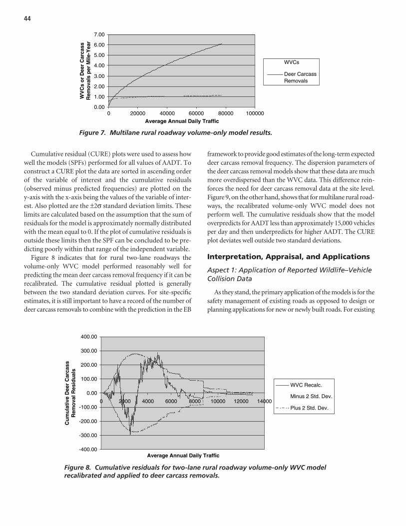
44

WVCs

Deer CarcassRemovals

0.00

1.00

2.00

3.00

4.00

5.00

6.00

7.00

0 20000 40000 60000 80000 100000

Average Annual Daily Traffic

WV

Cs

or

Dee

r C

arca

ssR

emo

vals

per

Mile

-Yea

r

Figure 7. Multilane rural roadway volume-only model results.

-400.00

-300.00

-200.00

-100.00

0.00

100.00

200.00

300.00

400.00

0 40002000 6000 8000 12000 1400010000

Average Annual Daily Traffic

Cu

mu

lati

ve D

eer

Car

cass

Rem

ova

l Res

idu

als

WVC Recalc.

Minus 2 Std. Dev.

Plus 2 Std. Dev.

Figure 8. Cumulative residuals for two-lane rural roadway volume-only WVC modelrecalibrated and applied to deer carcass removals.

Cumulative residual (CURE) plots were used to assess howwell the models (SPFs) performed for all values of AADT. Toconstruct a CURE plot the data are sorted in ascending orderof the variable of interest and the cumulative residuals(observed minus predicted frequencies) are plotted on they-axis with the x-axis being the values of the variable of inter-est. Also plotted are the ±2σ standard deviation limits. Theselimits are calculated based on the assumption that the sum ofresiduals for the model is approximately normally distributedwith the mean equal to 0. If the plot of cumulative residuals isoutside these limits then the SPF can be concluded to be pre-dicting poorly within that range of the independent variable.

Figure 8 indicates that for rural two-lane roadways thevolume-only WVC model performed reasonably well forpredicting the mean deer carcass removal frequency if it can berecalibrated. The cumulative residual plotted is generallybetween the two standard deviation curves. For site-specificestimates, it is still important to have a record of the number ofdeer carcass removals to combine with the prediction in the EB

framework to provide good estimates of the long-term expecteddeer carcass removal frequency. The dispersion parameters ofthe deer carcass removal models show that these data are muchmore overdispersed than the WVC data. This difference rein-forces the need for deer carcass removal data at the site level.Figure 9, on the other hand, shows that for multilane rural road-ways, the recalibrated volume-only WVC model does notperform well. The cumulative residuals show that the modeloverpredicts for AADT less than approximately 15,000 vehiclesper day and then underpredicts for higher AADT. The CUREplot deviates well outside two standard deviations.

Interpretation, Appraisal, and Applications

Aspect 1: Application of Reported Wildlife–VehicleCollision Data

As they stand, the primary application of the models is for thesafety management of existing roads as opposed to design orplanning applications for new or newly built roads. For existing

45

Annual Average Daily Traffic

Cu

mu

lati

ve D

eer

Car

cass

Rem

ova

l Res

idu

als

-1600.00

-1400.00

-1200.00

-1000.00

-800.00

-600.00

-400.00

-200.00

0.00

200.00

400.00

0 10000 20000 30000 40000 50000 60000 70000 80000 90000

WVC Recalc.

Minus 2 Std. Dev.

Plus 2 Std. Dev.

Figure 9. Cumulative residuals for multilane rural roadway volume-only WVC modelrecalibrated and applied to deer carcass removals.

roads, WVC data are available and used, along with the modelpredictions in an empirical Bayes procedure to estimate the ex-pected long-term mean collision frequency of a specific roadwaysegment. The following three types of model applications, whichwould be most relevant to the development of the desired guide-lines, are summarized and illustrated in the sections to follow:

• Network screening to identify roadway segments that maybe good candidates for WVC countermeasures,

• Evaluation of the effectiveness of implemented counter-measures, and

• Estimation of the cost effectiveness of potential counter-measures.

Network screening to identify roadway segments thatmay be good candidates for wildlife–vehicle collision coun-termeasures. Two fundamental methodologies are pre-sented and illustrated for this application:

• Identifying and ranking sites based on a high expectedfrequency of WVCs, and

• Identifying and ranking sites based on a high proportion ofWVCs

SPFs are used in the first application. The second applies forsituations where an SPF may not be available or applicable.

Identifying and ranking sites based on a high long-term fre-quency of wildlife–vehicle collisions. As noted earlier, the short-term collision count at a location is not a good estimate of itssafety. Thus, identifying and ranking collision-prone locationsbased on short-term counts will be inaccurate. Longer termcollision frequency data are now recognized as the best basis foridentifying and ranking these locations.

The long-term frequency of WVC data at a site is obtainedby using the EB methodology that combines the site’s WVC

frequency with the frequency expected by applying the SPFsdescribed earlier. In this approach, overlapping segments ofequal length should be considered in what is often termed a“sliding window” approach. A brief overview of the methodis provided with an example calculation. When the SafetyAn-alyst (www.safetyanalyst.org) software becomes available,there will be a facility to consider segments of different lengthusing a sophisticated “peak searching” algorithm.

In the EB procedure, the SPF is used to first estimate thenumber of collisions that would be expected at locations withtraffic volumes and other characteristics similar to the onesbeing analyzed. The estimate (P) is then combined with thecount of collisions (x) observed to obtain an estimate of theexpected number of collisions (m). This estimate of m is:

m = w1(x) = w2(P),

where the weights (w1 and w2) are estimated from the meanand variance of the SPF estimate as:

w1 = P/(P + 1/k)

w2 = 1/k/(P + 1/k),

and where k is the dispersion parameter for a given model andis estimated from the SPF calibration process with the use ofa maximum likelihood procedure. In this process, a negativebinomial distributed error structure is assumed with k beingthe dispersion parameter of the distribution. For networkscreening purposes, each segment is then ranked in descend-ing order by the expected number of collisions (m).

As an illustration, suppose that the two-lane rural roads inUtah are divided into 1-mi WVC segments that may or maynot overlap. Consider one such segment for which the fol-lowing information applies:

• Length = 1 mi (1.6 km)• Years of data = 16

46

Site Rank by EB Method

Rank by Proportions Method

11430 1 9 10194 2 6

9463 3 3 10336 4 48 11546 5 11

9947 6 4 9154 7 2

10177 8 5 6749 9 1 6716 10 35

11545 11 19 11554 12 12 10195 13 7 10197 14 8 11432 15 47

6697 16 28 9477 17 920

10673 18 18 6752 19 80 6694 20 86

Table 20. Comparison of alternative ranking methods.

• WVCs observed = 40• Average AADT = 2,066

First, the UT 1 model from Table 12 is used for this exampleto calculate the regression estimate (P).

Next, the weights (w1 and w2) are calculated.

w1 = 4.36/(4.36 + 1/1.7610) = 0.88

w2 = 1/1.7610/(4.36 + 1/1.7610) = 0.12

Last, the regression estimate (P) and the observed collisioncount (x) are combined.

m = 0.88(40) + 0.12(4.36) = 35.72

The EB estimate of the expected number of collisions dur-ing the 16-year period is 35.72, lower than the observed countof 40. This EB estimate is used in ranking this location rela-tive to the other 1-mi segments.

Identifying and ranking sites based on a high proportionof wildlife–vehicle collisions. Where traffic volume andother characteristics necessary to estimate the expected colli-sion frequency at a site are unavailable, identifying sites witha high proportion of WVCs might be appropriate. Thismethod uses the observed counts for WVCs and all collisionsat a site but adjusts for the “noise” in each of these counts. Forexample, one is more certain that the proportion is high fora site with 20 WVCs out of 30 collisions than for a site with2 WVCs out of 3 collisions. The theory behind this method isdescribed in Appendix C. Of particular note is that themethod only requires the counts of WVCs and all collisionsat sites to be screened (i.e., SPFs are not required). Thismethod is also being implemented in SafetyAnalyst.

By way of illustration, the Utah two-lane rural roadwaydataset is used. The data were manipulated into 1-mi longsegments, although any desired length could be considered.All sites were ranked by the two methods. The top 20 sitesranked using the EB estimate of mean WVC frequency out-lined earlier are presented in Table 20.

The same segments were also screened based on the prob-ability that their proportion of WVCs is greater than 20.7%,the mean proportion for all segments. The rankings fromthis “proportions” method are shown in the last column ofTable 20. As seen, seven of the top ten segments identifiedby the EB method were also in the top ten ranked bythe proportions method. Thirteen of the top twenty seg-ments identified by the EB method were also in the toptwenty ranked by the proportions method. It appears thatranking by a high proportion of WVCs may be a reasonable

P = − =( )( )exp( . )( , ) ..16 1 9 1135 2 066 4 361 0237

P = ( )( ) ( )years length AADTα β1

alternative to ranking by the EB estimate of WVCs if therequired data or resources are not available for developingor applying SPFs.

Evaluation of the safety effectiveness of implementedcountermeasures, specifically the installation of animalcrossings. The methodology for the conduct of a properobservational before-after study is well documented in alandmark book by Hauer.114 The statistically defendable before-after analysis methodology proposed overcomes thedifficulties associated with simple before-after comparisonsof collision counts. The proposed methodology:

• Properly accounts for regression-to-the-mean,• Overcomes the difficulties of using collision rates in nor-

malizing for traffic volume differences between the beforeand after periods,

• Reduces the level of uncertainty in the estimates of safetyeffects,

• Provides a foundation for developing guidelines for esti-mating the likely safety consequences of installing a cross-ing and fencing, and

• Properly accounts for differences in collision experienceand reporting practice in amalgamating data and resultsfrom diverse jurisdictions.

The task is to estimate what was the effect on safety ofinstalling wildlife crossing measures. In this, “safety” is theexpected number of WVCs per unit of time for a road seg-ment of interest. This estimate requires three steps:

47

1. Predict what safety would have been during the “after” pe-riod, had the status quo been maintained,

2. Estimate what safety was during the after period withcrossing measures in place, and

3. Compare the two.

The following approach to Step 1 (predicting what safetywould have been during the after period had the status quobeen maintained) is suggested:

• Account explicitly for the effect of changes in traffic flowby using an SPF;

• Account for the effect of weather, demography, and othervariables by using a comparison group to recalibrate theSPFs to be used; and

• Account for possible selection bias (regression-to-the-meaneffects) and improve estimation accuracy by the EB methodusing the best available methodology.114

In the EB approach, the change in safety for a given colli-sion type is given by:

λ−π

where λ is the expected number of collisions that would haveoccurred during the after period without the crossing measuresand π is the number of reported collisions during the afterperiod. In estimating λ, the effects of regression to the meanand changes in traffic volume are explicitly accounted for byusing SPFs relating collisions of different types and severities totraffic flow and other relevant factors for each jurisdictionbased on locations without crossing measures. The exposure ofanimals to the roadway is not accounted for.

In the EB procedure, the SPF is used to first estimate thenumber of collisions that would be expected during thebefore period at locations with traffic volumes and othercharacteristics similar to the one being analyzed. The esti-mate (P) is then combined with the count of collisions (x)during the before period at a treatment site to obtain an es-timate of the expected number of collisions (m) before thecrossing measures were installed. This process is identical tothat presented earlier, but is repeated here for completeness.This estimate of m is:

m = w1(x) + w2(P)

where the weights (w1 and w2) are estimated from the meanand variance of the SPF estimate as:

w1 = P/(P + 1/k)

w2 = 1/k/(P + 1/k)

and where k is the dispersion parameter for a given model andis estimated from the SPF calibration process with the use of amaximum likelihood procedure. In that process, a negative bi-

nomial distributed error structure is assumed with k being thedispersion parameter of this distribution.

The variance of the estimate (m) is:

Var(m) = ((x + 1/k)P2)/(1/k + P)2

A factor f is then applied to m to account for the length of theafter period and differences in traffic volumes between thebefore and after periods. This factor is the value of the SPFprediction for the after period divided by P:

f = sum of SPF predictions post treatment/P

The result, after applying this factor, is an estimate of λ. Theprocedure also produces an estimate of the variance of λ.

Var(λ) = (f/P)2Var(m)

The estimate of λ is then summed over all locations in a treat-ment group of interest (to obtain λsum) and compared withthe count of collisions during the after period in that group(πsum). The variance of λ is also summed over all sections inthe treatment group.

The Index of Effectiveness (θ) is estimated as:

θ = (πsum/λsum) / {1 +[Var(λsum)/(λsum2]}

The standard deviation of θ is given by:

Stddev(θ) = [θ2{[Var(πsum)/πsum2] +

[Var(λsum)/(λsum2]}/[1 + Var(λsum)/λsum

2]2]0.5

The percent change in collisions is in fact 100(1 − θ); thus, avalue of θ = 0.7 with a standard deviation of 0.12 indicates a30% reduction in collisions with a standard deviation of 12%.

As an illustration of the method, Table 21 presents the re-sults of an analysis for two sites located in Utah (U.S. Hwy 40between mileposts 4.0 and 8.0, and Utah Route 248 betweenmileposts 3.3 and 13.5). Each site involved the constructionof one or more at-grade wildlife crossings and continuousexclusion fencing that extended beyond the limits of thecrossings themselves. Note that the roadway inventory datahas divided these sections of the road into multiple subseg-ments due to differences in number of lanes, AADT, andother variables.

The results for the demonstrative case indicate a WVCreduction of:

(1 − 0.702) * 100 = 29.8% with a standard error of 9.1%

Note that this result is based on only two sites in one state andthus should not be used as conclusive evidence of the safetybenefits of installing wildlife crossings and fencing.

Estimation of the cost effectiveness of a potential coun-termeasure, such as a crossing. The objective is to pro-vide designers and planners with a guide to estimate thechange in WVC frequency expected with the installation of

48

SiteNo. of Lanes Length Years

BeforeYearsAfter

AADT Before

AADT After

Crashes Before (x)

Crashes After ( )

Sum of SPF Predictions

After k w1 w2 m Var (m) Var ( )

1 4 2.04 9 6 7654 13227 39 18 18.85 1.53 0.97 0.03 38.52 32.69 37.42 26.96 1 4 1.96 9 6 7450 13227 45 47 18.11 1.53 0.97 0.03 44.28 38.04 42.96 31.69 2 2 0.05 4 6 2630 7493 1 1 0.36 1.76 0.13 0.87 0.20 0.87 0.03 0.48 2 2 0.19 4 6 2630 7493 0 0 1.37 1.76 0.36 0.64 0.20 0.88 0.07 1.38 2 2 0.58 4 6 2630 7493 2 5 4.19 1.76 0.63 0.37 1.61 7.06 1.01 19.39 2 3 0.18 4 6 2630 7493 0 2 1.30 1.76 0.34 0.66 0.19 0.85 0.07 1.28 2 4 0.21 4 6 2630 7493 3 2 1.24 1.53 0.44 0.56 1.62 3.86 0.72 4.07 2 4 0.12 4 6 2553 7493 3 2 0.71 1.53 0.31 0.69 1.13 2.73 0.35 2.04 2 4 1.40 4 6 1707 3375 3 6 5.80 1.53 0.81 0.19 2.97 6.03 2.42 9.95 2 4 0.07 4 6 1707 3375 0 0 0.29 1.53 0.18 0.82 0.12 0.24 0.02 0.09 2 4 0.42 4 6 1707 3375 4 2 1.74 1.53 0.57 0.43 2.64 5.36 1.50 6.17 2 3 2.70 4 6 1707 3375 16 17 8.62 1.76 0.83 0.17 13.82 41.66 11.53 104.77 2 4 0.34 4 6 1707 3375 8 2 1.41 1.53 0.52 0.48 4.47 9.05 2.30 9.46 2 4 0.08 4 6 1707 3375 0 1 0.33 1.53 0.20 0.80 0.13 0.26 0.03 0.11 2 3 3.09 4 6 1707 3375 10 21 9.86 1.76 0.85 0.15 9.00 27.14 7.67 69.71 2 2 0.77 4 6 1707 3375 0 0 2.46 1.76 0.59 0.41 0.33 1.01 0.20 1.79 SUM 126 121.26 177.74 289.36 0.702 VAR( ) 0.008 S.E.( ) 0.091

Table 21. Illustration of EB before-after study for U.S. Highway 40 and Utah Route 248 in Utah.

49

wildlife crossings and fencing at a segment of roadwayunder consideration.

For the approach, an SPF representative of the existingroad segment is required. Therefore, an SPF must alreadyexist for the jurisdiction or data must be available to enable arecalibration of a model calibrated for another jurisdiction.The SPF would be used, along with the segment’s collisionhistory, in the EB procedure to estimate the expected collisionfrequency with the status quo in place; that estimate of colli-sion frequency would then be compared to the expectedfrequency if a crossing and fencing were constructed in orderto estimate their benefits.

This model application requires four steps:

1. Assemble data and collision prediction models for roadsegments:a. Obtain the count of WVCs;b. For each year, obtain or estimate the average AADT;

andc. Estimate the AADT that would prevail for the period

immediately after construction.2. Use the EB procedure documented earlier, with the data

from Step 1, and the road segment model to estimate the ex-pected annual number of WVCs that would occur withoutconstruction of the crossing and fencing.

3. Apply a Collision Modification Factor (CMF) to the ex-pected collision frequency with the status quo in place toget the expected benefit in terms of the number of annualWVC expected to be reduced. A CMF is an adjustment tothe estimate based on the expected reduction in WVCs.Until a reliable CMF can be determined from properlyconducted before-after studies, an interim CMF could bedeveloped through an expert panel as has been done forother roadway safety countermeasures. 113

4. Compare against the cost, considering other impacts ifdesired, and using conventional economic analysis guides.The results of the analysis above may indicate that crossingsare justified based on a consideration of safety benefits. Thisjustification should not be taken to mean that crossingsshould be constructed, because:a. Other measures may have higher priority in terms of

cost effectiveness,b. The safety benefits may need to be assessed in the light

of other impacts, andc. Other locations may be more deserving of a crossing. In

other words, the results of the above analysis should befed into the safety resource allocation process.

As an illustration, suppose a 2-mi long section of road,with data from 1998 to 2002, is being considered for the con-struction of a wildlife crossing and fencing along the entiresection. This section experienced 18 WVCs during this time

period. The average AADT was observed to be 5,000 and isassumed to increase by 5% following the proposed construc-tion, although this anticipated increase in traffic is not relatedto the contemplated construction. The SPF to be used is:

Use the EB procedure to estimate the expected annual num-ber of WVCs that would occur without construction of thecrossing and fencing.

w1 = 6.74/(6.74 + 1/1.6098) = 0.92

w2 = 1/1.6098/(6.74 + 1/1.6098) = 0.08

Last, the regression estimate (P) and the observed collisioncount (x) are combined.

m = 0.92(18) + 0.08(6.74) = 17.1, or 3.4/year

The combination of a high dispersion parameter (k) and rel-atively long length of the segment leads to a relatively highweight being given to the SPF estimate (P).

Because traffic is expected to increase 5% in the periodafter the contemplated construction the estimate (m) isadjusted by the ratio of the AADT term in the model:

m* = 3.4*(5000 * 1.05)1.0237/(5000)1.0237 = 3.57/year

An appropriate CMF is applied to the estimate (m* ) to esti-mate the expected benefit in terms of the number of annualWVCs expected to be reduced. For this illustration assumethat the expected reduction is 20% (i.e., that the CMF is(100-20)/100 = 0.8).

Annual Benefit = 0.20(3.57) = 0.71 wildlife–vehicle collisions

Apply the estimated cost per collision to the previously esti-mated annual WVC benefit to estimate the dollar value benefitper year. Compare this benefit against the annualized cost ofconstruction, maintenance, and other relevant considerations.

Aspect 2: Comparison of Wildlife–Vehicle Collisionand Carcass Removal Data

The primary objective of this aspect of the safety data analy-sis was to investigate the hypothesis that the choice and appli-cation of reported WVC and carcass removal data (as theymight exist and could be plotted at a DOT) could result invarying policies or WVC countermeasure-related roadway de-velopment decisions. One or both of these two databases havebeen used in the past to describe the magnitude of the WVCproblem and to propose and evaluate the effectiveness ofWVC countermeasures. Overall, the visual and quantitativefindings of the reported WVC and deer carcass removal com-parison activities revealed that both their magnitudes and

P = − =( )( )exp( . )( , ) ..5 2 9 1135 5 000 6 741 0237

P k= −( )( )exp( . )( ) ;.years length AADT9 1135 1 0237 == 1 6098.

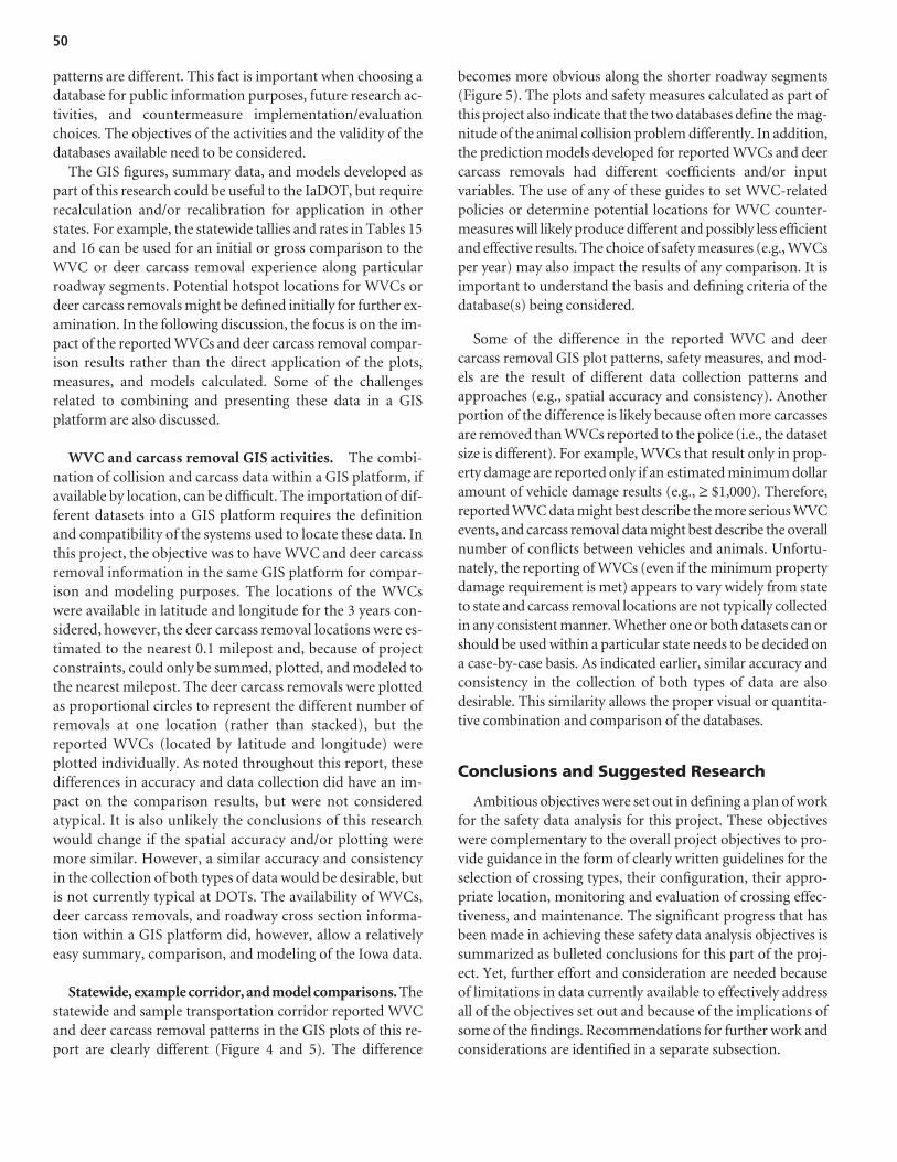
50

patterns are different. This fact is important when choosing adatabase for public information purposes, future research ac-tivities, and countermeasure implementation/evaluationchoices. The objectives of the activities and the validity of thedatabases available need to be considered.

The GIS figures, summary data, and models developed aspart of this research could be useful to the IaDOT, but requirerecalculation and/or recalibration for application in otherstates. For example, the statewide tallies and rates in Tables 15and 16 can be used for an initial or gross comparison to theWVC or deer carcass removal experience along particularroadway segments. Potential hotspot locations for WVCs ordeer carcass removals might be defined initially for further ex-amination. In the following discussion, the focus is on the im-pact of the reported WVCs and deer carcass removal compar-ison results rather than the direct application of the plots,measures, and models calculated. Some of the challengesrelated to combining and presenting these data in a GISplatform are also discussed.

WVC and carcass removal GIS activities. The combi-nation of collision and carcass data within a GIS platform, ifavailable by location, can be difficult. The importation of dif-ferent datasets into a GIS platform requires the definitionand compatibility of the systems used to locate these data. Inthis project, the objective was to have WVC and deer carcassremoval information in the same GIS platform for compar-ison and modeling purposes. The locations of the WVCswere available in latitude and longitude for the 3 years con-sidered, however, the deer carcass removal locations were es-timated to the nearest 0.1 milepost and, because of projectconstraints, could only be summed, plotted, and modeled tothe nearest milepost. The deer carcass removals were plottedas proportional circles to represent the different number ofremovals at one location (rather than stacked), but thereported WVCs (located by latitude and longitude) wereplotted individually. As noted throughout this report, thesedifferences in accuracy and data collection did have an im-pact on the comparison results, but were not consideredatypical. It is also unlikely the conclusions of this researchwould change if the spatial accuracy and/or plotting weremore similar. However, a similar accuracy and consistencyin the collection of both types of data would be desirable, butis not currently typical at DOTs. The availability of WVCs,deer carcass removals, and roadway cross section informa-tion within a GIS platform did, however, allow a relativelyeasy summary, comparison, and modeling of the Iowa data.

Statewide, example corridor, and model comparisons. Thestatewide and sample transportation corridor reported WVCand deer carcass removal patterns in the GIS plots of this re-port are clearly different (Figure 4 and 5). The difference

becomes more obvious along the shorter roadway segments(Figure 5). The plots and safety measures calculated as part ofthis project also indicate that the two databases define the mag-nitude of the animal collision problem differently. In addition,the prediction models developed for reported WVCs and deercarcass removals had different coefficients and/or inputvariables. The use of any of these guides to set WVC-relatedpolicies or determine potential locations for WVC counter-measures will likely produce different and possibly less efficientand effective results. The choice of safety measures (e.g., WVCsper year) may also impact the results of any comparison. It isimportant to understand the basis and defining criteria of thedatabase(s) being considered.

Some of the difference in the reported WVC and deercarcass removal GIS plot patterns, safety measures, and mod-els are the result of different data collection patterns andapproaches (e.g., spatial accuracy and consistency). Anotherportion of the difference is likely because often more carcassesare removed than WVCs reported to the police (i.e., the datasetsize is different). For example, WVCs that result only in prop-erty damage are reported only if an estimated minimum dollaramount of vehicle damage results (e.g., ≥ $1,000). Therefore,reported WVC data might best describe the more serious WVCevents, and carcass removal data might best describe the overallnumber of conflicts between vehicles and animals. Unfortu-nately, the reporting of WVCs (even if the minimum propertydamage requirement is met) appears to vary widely from stateto state and carcass removal locations are not typically collectedin any consistent manner. Whether one or both datasets can orshould be used within a particular state needs to be decided ona case-by-case basis. As indicated earlier, similar accuracy andconsistency in the collection of both types of data are alsodesirable. This similarity allows the proper visual or quantita-tive combination and comparison of the databases.

Conclusions and Suggested Research

Ambitious objectives were set out in defining a plan of workfor the safety data analysis for this project. These objectiveswere complementary to the overall project objectives to pro-vide guidance in the form of clearly written guidelines for theselection of crossing types, their configuration, their appro-priate location, monitoring and evaluation of crossing effec-tiveness, and maintenance. The significant progress that hasbeen made in achieving these safety data analysis objectives issummarized as bulleted conclusions for this part of the proj-ect. Yet, further effort and consideration are needed becauseof limitations in data currently available to effectively addressall of the objectives set out and because of the implications ofsome of the findings. Recommendations for further work andconsiderations are identified in a separate subsection.

51

Conclusions

Aspect 1: Application of reported wildlife–vehicle colli-sion data. This aspect of the work involved the develop-ment of safety performance functions and illustrated theirpotential applications related to the objectives of the project,rather than investigative research. Nevertheless, a few con-clusions may be drawn:

• Safety performance functions were successfully calibratedfor four states (in addition to that calibrated for Aspect 2) torelate police-reported wildlife–vehicle collisions to variablesnormally available in state DOT databases. For these func-tions, AADT was the dominant variable, with additional sig-nificant variables, such as speed, lane and shoulder width,and median type, making relatively small contributions tothe explanatory power of the SPFs.

• The SPFs varied considerably across states in terms of theeffect of the key AADT variable.

• The empirical Bayes procedure can be used to combineSPF predictions with WVC history to better estimate a lo-cation’s safety in accounting for key factors such as animalmovements not in the SPFs.

• The empirical Bayes estimate can be used for screening theroad network to identify candidate locations for WVCcountermeasures. However, for situations where SPFs, orthe resources required to calibrate them, are not available,a method that ranks locations according to their propor-tion of WVCs can produce reasonable results.

An illustration was presented of the application of SPFsin an empirical Bayes before-after study of safety effective-ness of a wildlife crossing installation. Sufficient installationdata were not available to enable the formal study that wasenvisaged.

Aspect 2: Comparison of wildlife–vehicle collision andcarcass removal data. The following conclusions are basedon the data combination, comparison, and analysis activitiespreviously described. The general objective of these activitieswas to visually and quantitatively determine whether the useof WVC and deer carcass removal data might lead to theidentification of different roadway segments for potentialcountermeasure implementation.

• Police-reported WVC and/or deer–vehicle collision(DVC) data by roadway location are available throughoutthe United States, but animal or deer carcass removal databy location are rarely collected and/or summarized.Carcass removal data may sometimes be available forshort periods of time and/or for specific roadway seg-ments, but is not typically collected consistently through-out a state for many years. Both of these databases can be

used to define the WVC problem, but the results will oftendiffer.

• The WVC and deer carcass removal data used in thisresearch was obtained from the IaDOT. These two datasetswere collected with different methods and at different lev-els of accuracy. This situation is not surprising, but it didlead to some challenges related to their combination andcomparison in a GIS platform. The WVC data from 2001to 2003 was available by latitude and longitude, but thedeer carcass removal locations were adjusted to the closestmilepost and summed. The impacts of modifying the deercarcass removal locations on the results of this research arenoted where appropriate.

• A quantitative summary of the 2001 to 2003 WVC and deercarcass removal data used in this research confirmed thatthere is a difference in their magnitude. There are more deercarcasses removed than WVCs reported. In addition, andnot surprisingly, the WVC and deer carcass removal data arecollected from different types of roadways. IaDOT primarilyremoves deer carcasses from interstates and U.S. Highways.A greater percentage of the police-reported WVCs occur onfarm to market routes and local roadways.

• A visual comparison of statewide and regional WVC anddeer carcass removal plots support the hypothesis that thedata from these two databases may result in the identifica-tion of different roadway segments as potential locations ofconcern. A similar comparison along example segments ofInterstate 80 and U.S. Highway 18 resulted in the sameconclusion. A quantitative comparison of the WVC anddeer carcass removal safety measures along these segmentsto relevant statewide calculations also supported the con-clusion that the choice of dataset (e.g., WVC or deercarcass removal) does matter. In addition, and notsurprisingly, the choice of the safety measure used in thecomparison also has an impact. The data used, type ofsafety measure calculated, and the analysis approachapplied all impact how “high” collision locations are iden-tified. Some of the differences observed in the data and themodels developed are caused by the dissimilarity in the ac-curacy and plotting approach of the WVC and deer carcassremoval data used.

• WVC and deer carcass removal regression models werecreated for rural two-lane and multilane roadways. Therural two-lane and multilane roadway WVC and deercarcass removal models have different coefficientsand/or variables. The results of these WVC and deer car-cass removal prediction models would be different forthe same roadway segment. This difference could impactdecisions related to countermeasure implementation.Overall, the WVC models generally had better explana-tory value than the deer carcass removal models, and thedeer carcass removal models should be used with caution

52

due to their high overdispersion parameters. The WVC anddeer carcass removal models that included only AADT didnot appear to be dramatically different in their predictivecapability than the models that included additional crosssection variables. The proper use and calibration of thesemodels is explained in other sections of this report.

• There is some potential to the use of WVC predictionmodels for the estimation of deer carcass removals alonga roadway segment, but a suitable database of deer carcassremovals needs to be available for recalibrating the WVCmodel. More research is needed on the value of this typeof application.

Recommendations

Aspect 1: Application of reported wildlife–vehicle colli-sion data.

• Empirical Bayes procedures, using the safety performancefunctions presented and police-reported WVCs (whereaccurate carcass removal data are unavailable), can be usedfor several tasks related to the project objectives:– Network screening to identify candidate roadway

segments for WVC countermeasures;– Evaluation of the safety effectiveness of wildlife crossing

installation and other WVC countermeasures; and– Estimation of the cost effectiveness, specifically the

safety benefits, of a contemplated wildlife crossing orother WVC countermeasure.

• Sufficient data should be collected to enable a full study ofthe safety effectiveness of crossings installed, using themethodology illustrated in previous sections. A minimumof 20 installations should provide useful results.

• An expert panel, similar to panels conducted recently fortraffic engineering countermeasures under NCHRP 17-25,should be convened to develop collision modification fac-tors for WVC countermeasures. These factors are used toestimate the safety benefits of a contemplated wildlifecrossing or other WVC countermeasure.

• For application in states other than those for which SPFsare presented, it is most desirable to develop SPFs for thatstate’s data. Where such development is not possible, anSPF from one of the four states for which SPFs arepresented can be applied, but it should be recalibrated toreflect differences across time and space in factors such ascollision reporting practices, weather, driver demograph-ics, and off-roadway variables such as wildlife movements.A procedure for doing this recalibration is presented inAppendix A. To determine which of the four models isbest to adopt for another state, some goodness-of-fit testswill need to be conducted. A summary of these tests ispresented as part of Appendix B.

Aspect 2: Comparison of wildlife–vehicle collision andcarcass removal data.

• The use of police-reported WVCs to identify potentialcountermeasure locations may only define a portion of astatewide or corridor-specific wildlife collision problem.The locations identified as “high” reported WVC locationsmay not be the same as those identified as “high” wildlifeor deer carcass removal locations.

• Currently, some type of police-reported animal–vehicle/deer–vehicle collision (AVC/DVC) data is typically avail-able at every state transportation agency. The total numberand location of deer carcass removals, on the other hand,are rarely collected consistently statewide. For this type ofsituation, the research team recommends that reportedAVC/DVC data should be used if safety improvements arethe primary objective, and deer or animal carcass removaldata (if not available by roadway location) should be usedfor public education and to describe the magnitude of theanimal collision problem from an ecological point of view.However, when the following recommendation is accom-plished, a more well-defined application of both databaseswould be desirable.

• The collection of statewide or corridor-specific WVCs orDVCs and large-animal carcass removal locations is rec-ommended to define the magnitude and patterns of thesafety concerns related to this issue. The consistent collec-tion and plotting of both types of data with the same spa-tial accuracy is desirable.

• When feasible and available, both WVCs or DVCs andlarge-animal carcass removal locations are recommendedfor use in combination to help define the magnitude andpatterns of this safety concern both statewide and alongspecific corridors. However, the double counting of animal–vehicle collisions should be avoided; e.g., deer car-cass removals should be ignored that occur at the sametime and location as a reported WVC or DVC. In this case,the attributes collected with the animal or deer removal(e.g., gender, estimated age, and species) might be trans-ferred, if possible, to the reported WVC database.

• The models developed in this research are recommended foruse only after they are appropriately calibrated and the usersunderstand the limitations of the models. The results ofthese models should be appropriately applied within an em-pirical Bayesian approach. The empirical Bayesian approachand model calibration of these types of models are explainedwithin several sections and appendices of this report. Thedevelopment of AVC/DVC models with more reported andcarcass removal data is also recommended. Models that ad-just for the severity (e.g., property-damage-only, injury, andfatality) of the large-animal– or deer–vehicle collisions mayalso be useful (if there is enough variability in this collisioncharacteristic). In general, it might be assumed that deer or

53

animal carcass removals that were not the result of a re-ported WVC or DVC were likely the outcome of a property-damage-only collision whose value did not require it to bereported.

3.2 Limiting Effects of Roadkill Reporting Data Due to Spatial Inaccuracy

Introduction

Wildlife–vehicle collisions do not occur randomly alongroads but are spatially clustered190,124,51,134 because wildlifemovements tend to be associated with specific habitats, terrain,and adjacent land-use types. Thus, landscape spatial patternswould be expected to play an important role in determininglocations where the probability of being involved in awildlife–vehicle collision is higher compared to other loca-tions.95 Explanatory factors of wildlife roadkill locations andrates vary widely among species and taxa. To properly mitigateroad impacts for wildlife and increase motorist safety,transportation departments need to be able to identify whereparticular individuals, species, taxa, and vertebrate com-munities are susceptible to high roadkill rates along roads.Quality field data documenting locations and frequencies ofwildlife–vehicle collisions can offer empirical insights to helpaddress this challenging safety and ecological issue.

As part of maintaining state and provincial highway sys-tems, transportation departments often collect informationon the location of wildlife–vehicle collisions. Typically,maintenance personnel do not conduct routine surveys ofanimal roadkilled carcasses, but instead collect this infor-mation opportunistically while carrying out their dailywork. Occasionally the information may be referenced towildlife species and specific geographical landmarks such as1.0-mile-markers or 0.1-mile-markers; however, oppor-tunistically collected roadkill data are usually not spatiallyaccurate. One study has shown that errors in roadkillreporting may be 500 m or greater.53 The inherent spatialerror in most agency datasets limits the types of applicationsfor which the data are useful in transportation planning andmitigation efforts.

This report demonstrates how wildlife–vehicle collisioncarcass data can be analyzed to guide transportation manage-ment decision making and mitigation planning for wildlifecrossings. The research team investigated the relative impor-tance of factors associated with wildlife roadkills using two dif-ferent datasets: one with highly accurate (high-resolution)GPS location data (<_ 10 m error) representing an ideal situa-tion and another lower resolution dataset with high spatialerror (<_ 0.5 mi or 800 m = low resolution), which is referredto as “mile-marker” data and is more characteristic of the

datasets available from most transportation agencies. Thisreport illustrates how spatial accuracy of the data affects theprocess of identifying variables that contribute to wildlife–vehicle collisions. Based on these outcomes, the research teammakes recommendations for collecting roadkill data moresystematically and accurately, emphasizing the value of spatialaccuracy in identifying and prioritizing problematic areas forhighway mitigation projects. The intent of this effort is toprovide an overview of considerations regarding the qualityand application of wildlife–vehicle collision carcass data to aidin assessing and mitigating wildlife–vehicle collisions.

This study was conducted in the Central Canadian RockyMountains approximately 150 km west of Calgary, straddlingthe Continental Divide in southwestern Alberta and south-eastern British Columbia (Figure 10). The study area encom-passes 11,400 km2 of mountain landscapes in Banff, Kootenay,and Yoho national parks, and adjacent Alberta provinciallands. This region has a continental climate characterized bylong winters and short summers.121 Vegetation consists of openforests dominated by lodgepole pine (Pinus contorta), Douglasfir (Pseudotsuga menziesii), white spruce (Picea glauca), Engle-mann spruce (Picea englemannii), quaking aspen (Populustremuloides), and natural grasslands.

Geology influences the geographic orientation of the majordrainages in the region, characterized by valleys runningnorth to south and delineated by steep shale mountains. Ona regional scale, east-west movements of animals across andbetween these valleys are considered vital for long-term sus-tainability of healthy wildlife populations in the region. Thetransportation corridors associated with the major water-sheds influence the distribution and movement of wildlife inthe region. As the most prominent drainage, the Bow Valleyaccommodates the Trans-Canada Highway (TCH), one ofthe most important and, therefore, heavily traveled trans-portation corridors in the region.

Highways in the study area traverse montane andsubalpine ecoregions through four major watersheds in theregion (Figure 10). Table 22 describes the location and gen-eral characteristics of the five segments of highways that wereincluded in this study.

Research Approach: Methods and Data

Data Collection

Spatially accurate dataset. In August 1997, efforts wereinitiated to maximize data collection from carcasses resultingfrom WVCs and to improve the spatial accuracy (resolution)of reported locations of WVCs occurring on the highways inthe study area. The research team worked with the agenciesand highway maintenance contractors that were responsiblefor collecting and reporting wildlife carcasses, primarily elk.

54

Banff National Park

KootenayNational Park Kananaskis

Valley

Yoho National Park

Province

Figure 10. Location of Canadian study area.

a 2005 annual average daily traffic volume. Data from Parks Canada; Banff National Park; and Alberta Transportation, Edmonton, Alberta. b 1999 summer average daily traffic volume. Data from Alberta Transportation, Edmonton, Alberta.

Highway Watershed Province Road

Length(km)

TrafficVolume(ADT)

PostedVehicleSpeed(km/h)

Trans-CanadaHighway Bow River Alberta, East of Banff

National Park 37 16,960a 110

Trans-CanadaHighway Bow River Banff National Park,

Alberta 33 8,000a 90

Trans-CanadaHighway Kicking Horse River Yoho National Park,

British Columbia 44 4,600a 90

Highway 93 South Kootenay River Kootenay National

Park, British Columbia 101 2,000a 90

Highway 40 Kananaskis River Alberta 50 3,075b 90

Table 22. Characteristics of the major highways in the Canadian study area.

The agencies consisted of Parks Canada (Banff, Kootenay,and Yoho National Parks), Alberta Sustainable Resource De-velopment (Bow Valley Wildland Park, and KananaskisCountry) and Volker-Stevin, maintenance contractor for theTrans-Canada Highway east of Banff National Park in the

province of Alberta. This collaborative effort included na-tional park wardens, provincial park rangers, and mainte-nance crews of Volker-Stevin.

The research team provided colored pin-flags to markthe sites in the right-of-way where roadkilled wildlife were

55

observed and collected. After placing a pin-flag, collaboratorswere asked to report to the research team via telephone, fax,or email. Most wildlife carcasses were pin-flagged and re-ported within 48 hours.

The collaborators recorded the location of wildlife car-casses by describing the location with reference to a nearbylandmark (e.g., 0.3 km west of Banff National Park east en-trance gate). Each reported WVC carcass site was re-locatedand confirmed by measuring the odometer distance from thereported landmark to the pin-flagged site. Once the locationwas confirmed, researchers recorded the actual location inUniversal Transverse Mercator (UTM) grid coordinatesusing a differentially correctable GPS unit (Trimble Naviga-tion Ltd., Sunnyvale, California, USA) with high spatial ac-curacy (<_ 10 m). The UTM coordinates were recorded in adatabase along with the original date of each reported road-kill and information regarding the species, sex, age, and num-ber of individuals involved.

For this study, the research team used only ungulate car-cass data (UVC), because ungulate species composed 76% ofthe total wildlife mortalities. In addition, these species areoften the greatest safety concern to transportation agenciesgiven their size and relatively common occurrence in ruraland mountain landscapes. Ungulate species included white-tailed and mule deer (Odocoileus virginianus and Odocoileushemionus, respectively), unidentified deer (Odocoileus sp.),elk (Cervus elaphus), moose (Alces alces), and bighorn sheep(Ovis canadensis). The UVC data obtained from the methodsdescribed in the previous paragraphs are hereafter referred toas the “spatially accurate,” “high-resolution,” or “GPS”dataset and serve as a benchmark for the analysis.

Mile-marker dataset. To investigate the influence thatspatial accuracy and scale may have on the results and inter-pretation of the data, the research team created a mile-markerdataset using the spatially accurate dataset, but shifting eachUVC location to the nearest hypothetical mile-marker. To dothis, each of the five highways in the study area was divided into1.0-mile-marker segments using ArcView 3.3.77 All spatially ac-curate UVC data were plotted onto the road network and thenmoved to the nearest mile-marker reference point. Each ob-served data point was moved an average distance of 400.2 m ±218.8 m (min. 7.3, max. 793.9) to its nearest mile-marker. Theresearch team recorded the UTM coordinates of each mile-marker location and summed the number of UVCs in thatmile-marker segment, defined as 800 m (0.5 mi) up and downthe road of the given mile-marker. The UVC data adjusted tothe closest mile-marker are hereafter referred to as the “spa-tially inaccurate,” “low-resolution,” or “mile-marker” data.

High- and low-kill locations. The mean number of road-kills per mile were calculated for each highway and rounded

to the nearest whole number. Buffers of 800 m (0.5 mi) radiuswere generated around each mile-marker sampling site andeach highway segment within the buffer was categorized as ahigh-kill or low-kill zone. This categorization was determinedby comparing the total number of UVCs associated with asegment to the mean number of UVCs per mile for the samestretch of road for each of the five highways in the study area.If the summed number of UVCs associated with a single mile-marker segment was higher than the average calculated permile for the same highway, that mile-marker segment wasconsidered a high-kill zone. Similarly, if the summed numberof UVCs within a mile-marker segment was lower than the av-erage for that highway, the mile-marker segment was definedas a low-kill zone. Each spatially accurate UVC location wasclassified as a high-kill or low-kill zone according to whichmile-marker segment it fell within. For example, a mile-marker segment with greater than or equal to 2 roadkills onHighway 40 in Kananaskis was a high-kill zone, while asegment with less than 2 roadkills was a low-kill zone.

Variables and Models

Site-specific variables. The research team measured site-specific variables at 499 sites from the GPS data and 120 sitesfrom the mile-marker dataset between April 2003 and July2005. Only 499 UVC locations were used; 47 UVC reportsfrom Kootenay Highway 93 South were excluded becausethey occurred prior to the clearing of roadside vegetationalong a 24 km stretch of the Kootenay Highway 93 South.Using a differentially correctable GPS unit to locate each sam-pling site, the research team measured 14 variables to be usedas possible factors explaining UVC occurrence (Table 23). Arange finder (Yardage Pro® 1000, Bushnell® Denver, CO)measured distance to nearest vegetative cover, and the inlineand angular visibility measurements. Vegetative cover, habi-tat, topography, and slope were all estimated visually. Fieldvisibility variables estimated the extent to which a motoristcould see ungulates on the highway right-of-way, or con-versely, how far away an oncoming vehicle could be seenfrom the side of the highway. Field visibility was measured viaa rangefinder as the distance that an observer, standing at oneof three positions (edge of the pavement, 5 m from pavementedge, or 10 m from pavement edge), lost sight of a passingvehicle. This measurement represents the distance that an ap-proaching driver might be able to see an animal from theroad. Because in most cases it could not be determined fromwhat side a vehicle struck an animal, or in which direction thevehicle was traveling, four visibility measurements were takenat each position (two facing each direction of traffic on bothsides of the highway). These four measurements were aver-aged to provide mean values estimating visibility at the edgeof the road, 5 m away from the edge of the road, and 10 m

56

Variable Name Definition

Field variables

Habitat class* Dominant habitat within a 100 m radius on both sides of the highway measured as open (O): meadows, barren ground; water (W): wetland, lake, stream; rock (R); deciduous forest (DF); coniferous forest (CF); open forest mix (OFM)

Topography* Landscape scale terrain measured as flat (1), raised (2), buried-raised (3), buried (4), partially buried (5), partially raised (6)

Forest cover Mean percentage (%) of continuous forest cover (trees > 1 m height) in a 100 m transect line perpendicular to the highway, taken from both sides of the road

Shrub cover Mean percentage (%) of shrub cover (trees and shrubs < 1 m high) in a 100 m transect line perpendicular to the highway, taken from both sides of the road

Barren ground Mean percentage (%) of area devoid of vegetation (rock, gravel, water, pavement, etc.) in a 100 m transect line perpendicular to the highway, taken from both sides of the road

Vegetative cover Mean distance (m) to vegetative cover (trees and shrubs > 1 m high) taken from both sides of the road

Roadside slope Mean slope ( ) of the land 0–5 m perpendicular to the pavement edge taken from both sides of the road

Verge slope Mean slope ( ) of the land 5–10 m perpendicular to the pavement edge taken from both sides of the road

Adjacent land slope Mean slope ( ) of the land 10–30 m perpendicular to the pavement edge taken from both sides of the road

Elevation GPS height (m) Road width Distance (m) from one side of the highway pavement to the other In-line visibility field* Mean distance at which an observer standing at the pavement edge could no longer

see passing vehicles; taken from each direction on both sides of the highway Angular visibility 1 Mean distance at which an observer standing 5 m from the pavement edge could no

longer see passing vehicles; taken from each direction on both sides of the highway Angular visibility 2 Mean distance at which an observer standing 10 m from the pavement edge could

no longer see passing vehicles; taken from each direction on both sides of the highway

Distance-to-landscape features

Drainage Distance (m) to the nearest waterway (river, stream, or creek) that crossed the road Human use Distance (m) to the nearest human use feature along the highway Barrier-guardrail Distance (m) to the nearest Jersey barrier or guardrail

GIS-generated buffer variables

Road curvature Length (m) of each highway segment within each bufferOpen water Area (km2) of open water within each buffer Human use Area (m2) of human use features within each bufferRiver length The length (m) of all rivers within each buffer Barrier length The length (m) of all Jersey barriers and guardrails in each buffer

* Variable measure obtained from field measurement (1) flat (2) raised (3) buried-raised

(4) buried (5) partially buried (6) partially raised

Table 23. Definition and description of variables used.

from the edge of the road. These positions are defined as “in-line visibility,” “angular visibility 1,” and “angular visibility2,” respectively, as referred to in Table 23.

Spatial and elevation data were collected along each high-way approximately every 25 m, by driving at 50 km/h andrecording a GPS location every second. Elevation was ob-tained on site from a GPS unit for the spatially accurate datalocations, whereas elevation for the mile-marker points wasextracted from the GPS-created highway layer.

GIS-generated variables. Measurements for most vari-ables were obtained in the field; some were obtained using Ar-cView 3.3 GIS.77 Distance from each sampling site to landscape

features (Table 23) was calculated using GIS. The researchteam generated 800 m (0.5 mi) radius buffers around each spa-tially accurate and mile-marker sampling site and calculatedthe area or length of each landscape feature within each buffer.The road network was used to calculate the length of each high-way segment within each buffer to measure curvature of thehighway (Table 23).

Data Analysis

The research team tested whether the spatially accurateUVCs were distributed randomly by comparing the spatialpattern of collisions with that expected by chance, in which

57

case the likelihood of collisions for each road section wouldshow a Poisson distribution.32 For each of the four water-sheds, the research team classed the highways into segments100 m long and recorded presence (1) or absence (0) of theobserved UVC points in each segment. A Kolmogorov-Smirnov one-sample test was used to determine whether theempirical distribution differed from a Poisson distribution.Also a χ2 test based on overall highway length was used todetermine if an obvious UVC aggregation was significantalong the cleared section or low valley bottom of KootenayHighway 93 South. Finally, the research team determined theaggregation of UVCs along each highway (i.e., whether killswere evenly spread or clumped) by determining the percent-age of mile-markers associated with a UVC location.

Univariate analyses were used to identify which of thecontinuous variables (unpaired t-tests) and categorical vari-ables (χ2 contingency tests) differed significantly (P < 0.05)between high- and low-kill sites within the spatially accurateand mile-marker datasets. The significance of each differen-tiated class within the categorical variables was evaluatedusing Bailey’s confidence intervals.48

Logistic regression analyses were used to identify which ofthe significant parameters best predicted the likelihood of UVCoccurrence within the spatially accurate and mile-markerdatasets.123 Stepwise (backward) regression procedures wereused to remove variables from the equation until each result-ing model was not significantly more informative than theprevious one. The log-likelihood ratio test123 was used to de-termine the ability of each model to discriminate betweenhigh- and low-kill zones based on location attributes. Signifi-cance of explanatory variable coefficients was based on the χ2

of the Wald statistic.123 Standardized estimate coefficients werecalculated by multiplying logistic regression coefficients (B) bythe standard deviation of the respective variables. With this, theresearch team assessed the relative importance of the explana-tory variables within the model. Odds ratios were examined toassess the contribution that a unit increase in the predictorvariable made to the probability of a UVC occurring.229

Hosmer-Lemeshow goodness-of-fit test statistics were in-cluded to see how well the model predicted the dependent vari-able. To validate the high-resolution and mile-marker models,the research team generated cross-validation classification ac-curacies for each model. Both the high- and low-resolutionmodels were validated with a random subset of 20% of the datanot included in their development.

Prior to performing the regression analysis, the researchteam tested potential explanatory variables for multicollinear-ity.167 Where variables correlated (r > 0.7), the research teamremoved one of the two variables from the analysis. Finalmodels and variable coefficients with a P-value less than orequal to 0.1 were considered significant. The research teamused the SPSS statistical package version 11.0 for all statistical

analyses220, and Microsoft Excel and ArcView GIS 3.377 for allother analyses.

Findings and Results

Summary of Ungulate–Vehicle Collision Data

A total of 546 UVC observations were recorded betweenAugust 1997 and November 2003 on all highways in the studyarea. Deer (mule deer, white-tailed deer, and unidentifieddeer) were most frequently involved in collisions and com-posed 58% of the kills, followed by elk (27%), moose (7%)bighorn sheep (3%) and other ungulates, including moun-tain goats and unidentified species (5%).

The majority of UVCs occurred on the TCH east of BanffNational Park in the province of Alberta (46%), followed byHighway 93 South in Kootenay National Park (22%), High-way 40 in Kananaskis Country (12%), the TCH in Yoho Na-tional Park (10%), and the TCH in Banff National Park(10%). Calculating the average number of kills per mile foreach highway in the study area showed that the majority ofUVCs occurred on the TCH in the province of Alberta (13.6kills/mi), followed by the TCH in Banff National Park (2.6kills/mi), the TCH in Yoho National Park (2.1 kills/mi),Highway 40 in Kananaskis (2.1 kills/mi), and Highway 93South in Kootenay National Park (1.8 kills/mi). These UVCrates followed traffic volume trends, which were highest onthe TCH east of Banff National Park in the province of Al-berta, followed by the TCH in Banff National Park, TCH inYoho National Park, Highway 40 in Kananaskis Country, andHighway 93 South in Kootenay National Park.

Spatial Distribution of Roadkills

The accuracy of the location where site-related variables weremeasured for the spatially accurate locations was approximatelyless than or equal to 10 m. The UVC distributions from the spa-tially accurate dataset differed significantly from random distri-butions along all five highways in the study area (Kolmogorov-Smirnov one-sample test: TCH–Bow River Valley, d = 0.715;Highway 93 South in Kootenay, d = 0.940; TCH–Yoho, d =0.892; Highway 40 in Kananaskis, d = 0.874; all P < 0.01). Thedistribution of UVCs on Highway 93 South in Kootenayshowed a significant aggregated distribution where the highwaytraversed the low valley bottom with 60% of the kills occurringalong a 24 km (23%) stretch of road (χ2 = 63.9, P < 0.0001). TheTCH in Alberta had the majority of mile markers associatedwith a roadkill (89%), followed by the TCH in Banff NationalPark (86%), followed by Highway 40 (84%), followed by High-way 93 South in Kootenay National Park (61%), and the TCHin Yoho National Park (57%). Because of the non-random pat-tern and aggregation of UVCs, the research team explored

58

Spatially Accurate Mile-Marker VariableHigh Low P-value High Low P-value

Field variables

HabitatRockConiferous forest Open forest mix

2144112

11177

54

<0.0001

TopographyFlatBuried-raised

24132

17271

<0.000124 12

0.0035

Forest cover 46.7 53.3 0.0256 Openness 47.3 41.6 0.0496 Adjacent land slope 11.4 15.9 0.0059 Road width 34.1 24.8 0.0001 19.51 15.2 0.0300

Distance-to-landscape features

Drainages 2389.9 3068.9 0.0003 Barrier-guardrail 627.0 1052.2 0.0003

GIS-generated buffer variables

Barrier length 272.7 353.2 0.0182 336.51 548.4 0.0036 Open water 49.2 109.8 0.0001

This table shows a comparison using a spatially accurate dataset (n = 499; 391 high- and 108 low-density points) and mile-marker dataset (n = 120; 63 high- and 57 low-density points). Mean values are shown for quantitative variables, and frequencies for each differentiated type are shown for categorical variables, along with their associated P-values. Only those values that were significant at P < 0.05 are displayed.

Table 24. Univariate comparison of factors contributing to UVCs.

which landscape and road-related factors may be contributingto the distribution of collisions in the study area.

Models

Univariate tests. Table 24 shows the results of the uni-variate tests comparing high- and low-kill locations for eachenvironmental variable contributing to the probability ofUVCs in each dataset. Each dataset had variables in eachgroup that were significant in detecting differences betweenUVC high- and low-kill zones, however only three of ten vari-ables were significant in the mile-marker dataset.

Within the spatially accurate dataset, Table 24 shows thatsix of the field-based variables were significant: habitat class,topography, forest cover, openness, adjacent land slope, androad width. Only two of the field variables (road width andtopography) were significant from the mile-marker dataset.In both datasets, more UVCs occurred when the topographywas flat and the roads were wide. In the spatially accuratedataset, more UVCs occurred than expected in open foresthabitat and fewer UVCs occurred than expected in conifer-ous forest and rocky areas.

Within the landscape feature variables, distance to drainageand barrier-guardrail were significant (negatively correlated)in the spatially accurate dataset. More UVCs occurred than ex-pected closer to drainages perpendicular to the roadway andcloser to barriers-guardrails (including Jersey barriers). Nodistance-to-landscape features were significantly correlated tothe high- and low-kill zones in the mile-marker dataset.

Within the GIS-derived variables, areas of open watershowed a significant negative correlation to the dependentvariable in the spatially accurate dataset, while only the meas-ure of barrier length gave a significant negative correlation inboth datasets. Less open water and shorter lengths of barrierswere associated with high-kill zones.

To reduce intercorrelation between the variables,252 the re-search team omitted the percentage of forest cover from fur-ther analyses because it was highly correlated (r > 0.70) withpercentage of cleared ground.

Logistic regression analysis. Both models ranked differ-ently in their ability to predict the observed likelihood forUVCs (Table 25). The variables used in each model could col-lectively be used to predict where a UVC would occur for thespatially accurate model (P < 0.0001) but not for the mile-marker model (P = 0.584) as determined from the log likeli-hood ratio test. For the spatially accurate model, the Hosmer-Lemeshow statistic was higher than the mile-marker model.The predictive capabilities of the GPS model correctly classi-fied 81.8%, while the mile-marker model correctly classifiedonly 64.4% of the selected UVC data. Model validation accu-racies were 76.9% for the GPS model and 63.3% for the mile-marker model. Type of habitat was the most important vari-able in explaining UVCs in the GPS dataset. Ungulate–vehiclecollisions were less likely to occur near open water, deciduousforest, closed coniferous forest, and open forest mix relative toopen habitat. Kills were 2.7 times less likely to occur in water-dominated habitats (lakes, wetlands) relative to open habitat

59

Variable Spatially Accurate Mile-Marker Habitat Water 1– Coniferous forest 4– Deciduous forest 5– Open forest mix 2– Distance to drainage 3– Barrier-guardrail N/A+ Road width N/A+ Barrier length N/A– 1– Open water N/A– Hosmer–Lemeshow test 0.764 0.512 Model development & validation accuracies (%) 81.8 76.9 64.4 63.3

N/A = standard deviation in the logistic regression output was equal to 0

Table 25. Logistic regression analyses for modeling factors contributing to UVCs.

areas (dry meadows, clearings). Further, distance to drainagehad a significant negative correlation with the occurrence ofUVCs in the GPS model. The distance to barrier-guardrail andthe length of the barriers within the buffer both showed anegative correlation with UVCs. In the mile-marker model,barrier length showed a significant negative correlation withUVCs.

In Table 25, results are presented from the logistic regressionanalyses for modeling the factors contributing to UVCs usingtwo datasets. They include a spatially accurate dataset (n = 499locations; 391 high- and 108 low-density points) and a mile-marker dataset (n = 120; 63 high- and 57 low-density points).Also shown are their associated ranking of significant (P <0.10) standardized estimate coefficients and their sign. Num-bers indicate the rank of importance of the variable. The signindicates the influence the variable or variable level has on theprobability of a roadkill occurring [(–) negative correlation or(+) positive correlation]. Hosmer-Lemeshow goodness-of-fittest and overall cross-validation accuracies are included; theterm N/A means that the standard deviation in the logisticregression output was equal to 0.

Interpretation, Appraisal, and Applications

Summary of UVC Data

For this analysis, the research team used the largest data-base of its kind with spatially accurate information on theoccurrence and specific carcass location of WVCs. The traf-fic mortality database is also unique in that it spans arelatively short time period (1999–2005), whereas otherdatabases, regardless of their spatial accuracy, often containroadkill information from a decade or more. The short timespan used in this analysis is important because over longtime periods, environmental variables may change (e.g.,roadside vegetation and motorist visibility, habitat quality),as can road-related variables (e.g., guardrail and Jersey

barrier installation, road widening and improvements,lighting), thus confounding analysis and resulting in possi-ble spurious results.

Previous explanations for the clustering of WVCs includedparameters such as animal distribution, abundance, and dis-persal and road-related factors including local topography,vegetation, vehicle speed, and fence location or type.190,4,47

Few studies have demonstrated that WVCs were correlatedwith traffic volume.160,4,47,124 The majority of WVCs in theanalysis took place in the provincial section of the TCHfollowed by Highway 93 South in Kootenay National Park.However, when the roadkill frequencies were standardized byhighway length in the study area, the rate of roadkill wasfound to correlate positively with traffic volume.

Factors in addition to traffic volume may influence colli-sion rates, but may be masked if a more detailed and rigor-ous analysis is not conducted. Previous research in the sameCanadian study area found that elk–vehicle collision rateswere significantly different between road types and declinedover time on the TCH in Banff and Yoho National Parks,and Highway 93 South.53 In this analysis, when the effects oftraffic volume and elk abundance on elk–vehicle collisionrates were isolated, the latter was particularly important.53

Significant interactions indicated that road type influencedthese effects and greater elk abundance led to increasedelk–vehicle collisions. For this analysis, the research teamdid not include elk abundance as an independent variablebecause the elk abundance data available for analysis wasnot at the same spatial resolution as the site-specific loca-tions in the accurate UVC model. Of the five highways in-cluded in this study, the relative abundance of ungulates ishighest in the provincial section of the TCH and KootenayRiver Valley along Highway 93 South. The other highways(TCH-Banff, TCH-Yoho, and Highway 40) are situated athigher elevations and have lower ungulate densities. Fewstudies investigating factors influencing WVCs haveincluded data on animal abundance.20,190,53

60

Models of Ungulate–Vehicle Collisions

Spatial distribution and aggregation. The spatial distribu-tion of UVCs on all five highways in the study area was notrandom. The most notable aggregation was along the 24 kmstretch of highway on 93 South. This segment of highway bi-sects key ungulate ranges in the valley bottoms of the mon-tane region, with elevation less than 1240 m.188

Several environmental and road-related variables had highexplanatory power in describing UVCs on all highways, andthese variables were dependent on the spatial accuracy of thedataset. Results of the univariate analysis demonstrated thatthe GPS dataset had substantially more significant variables(n = 10 variables) explaining the factors associated with UVCsthan the mile-marker dataset (n = 3 variables).

Predictive ability of datasets. Univariate tests and logis-tic regression analysis were used to determine the predictiveability of the two datasets.

Univariate tests. Among the field-based variables, onlytwo were identified in the mile-marker dataset as being sig-nificant in detecting differences between high- and low-killUVC zones. The same variables were also identified amongthe six significant variables in the GPS dataset. Two of thevariables from the distance-to-landscape features and GIS-generated buffer variables were significant from the spatiallyaccurate dataset, whereas the mile-marker dataset had none.

Univariate tests are often used as a preliminary step toidentify one or more variables that are most likely good pre-dictors of responses to include in an a priori logistic regres-sion analysis.123 The results of the univariate tests of signifi-cance provide an interesting comparison of how well eachdataset is able to describe the relationship between predictorvariables and the location of UVCs. Of the 22 variables usedin the initial univariate test to identify variables that differedsignificantly between high- and low-kill UVC zones, 10(roughly half) of the spatially accurate variables compared toonly 3 (< 10%) of the mile-marker variables were statisticallysignificant (see Table 24).

Logistic regression analysis. Results of the logistic re-gression analysis to predict the likelihood of UVCs for the twodatasets analyzed in this study showed the GPS model wasstatistically significant, however, the mile-marker model wasnot. Further, both of the models differed considerably in howwell they predicted the likelihood of UVCs. Strong support ofthe predictive ability of the GPS model compared to the mile-marker model was found with the higher cross-validationscores. These results provide strong evidence that the GPS-collected data is more likely to be informative in explainingWVCs than the mile-marker data.

Factors that explain collisions. The spatially accuratemodel indicated that adjacent habitat type was the most im-portant variable in explaining UVCs. The proximity to openhabitat increased the likelihood of UVCs as opposed to habi-tats characterized by open water, deciduous forest, closedconiferous forest, and open forest mix. Gunther et al.109 re-ported that elk were involved in collisions significantly moreoften than expected in non-forested cover types. Manydeer–vehicle collisions in Pennsylvania were concentratedaround woodland-field interfaces in predominantly openhabitat.15 On the other hand, some studies have not foundthis association between habitat type and UVCs.4,25 Wildlifetends to be associated with specific habitats that provideresources and environmental conditions that promote occu-pancy and survival.176 Thus, the spatial distribution of habi-tat types adjacent to or bisected by a highway transportationcorridor would likely influence the extent, severity, and loca-tions of vehicle collisions with wildlife.

Landscape variables other than habitat and topography mayalso be important attributes determining UVCs. For example,distance to nearest drainage was significantly and negativelycorrelated with the occurrence of UVCs in the spatially accu-rate model. Ungulates had a greater tendency to be involved intraffic collisions close to drainage systems. Drainage systemsare known travel routes for wildlife, particularly in narrowglacial valleys such as Banff’s Bow Valley.51 Furthermore,research has shown that topography, particularly road align-ment with major drainages, strongly influences the movementof ungulates toward roadways and across them.20,45,159,86

The proximity to potential barriers such as Jersey barriersand guardrails was an important predictor of UVCs in thestudy area. The same result was found when measuring thelength of Jersey barrier or guardrail within the 800 m buffer inhigh- and low-kill UVC zones. UVCs were found to occurnearer to Jersey barriers and guardrails, which may be becauseanimals are funneled to the ends of the barriers and cross thehighway at this point. Furthermore, fewer animals were killedwhen the length of barriers within the 800 m buffer decreased.These results suggest that the barrier is obstructing animalmovement and funneling animals to barrier ends, or particu-lar features in the landscape associated with barriers such aslakes and steep topography are deterring animals from ap-proaching the highway at these locations. Barnum 14 foundthat animals crossed more frequently at culverts, bridges, andat-grade crossings with no guardrail or median barrier. Theonly study modeling AVCs that included guardrails in theanalysis also found that animals tended to avoid highwaysections with these potential barriers; i.e., collisions were lesslikely to occur where barriers were present.158

The results have important ecological implications becausethey suggest that median barriers and guardrails may obstructanimal movement across highways. Further, the results have

61

important management implications because state trans-portation agencies are constructing highway median barrierswith virtually no information on how they affect wildlifemovement and mortality. Despite these potential impacts,the 2003 AASHTO Roadside Design Guide does not addressthe impact of median barrier installation. Resource managersand transportation biologists have identified this lack as asevere shortcoming that needs immediate attention. A recentTransportation Research Board report highlighted the urgentneed to better understand how wildlife respond to and arepotentially impacted by highway barriers.233

Spatial accuracy and interpretation of results. In themile-marker dataset, few landscape variables were significant.For example, level or gentle topography due to flat terrain isbisected by the TCH in the province of Alberta. Further, roadwidth was a significant explanatory variable due to the widthand number of lanes of traffic on the TCH in the province ofAlberta. Both of these variables are not as dependent on spatialaccuracy, because they were broad-scale measurements withlow variability occurring on large sections of the highway.

None of the distance-to-feature variables showed signifi-cance in the mile-marker dataset. These types of variables arestrongly dependent on spatial accuracy of reporting UVCs.For example, if a UVC location has an error up to 800 m, itwill be evident in the measurement of these variables.

The GIS-generated buffer variables could be used to meas-ure factors associated with UVCs in a mile-marker dataset.158

The buffer encompasses the entire area in which the UVCswould have occurred, thus the factors associated with thatroadkill are incorporated into the measurement of thevariables. Barrier length was a significant explanatory variablein both datasets and area of open water was marginally signif-icant in the mile-marker dataset. These variables would haveto be a broad-scale landscape feature such as the area of afeature within the entire buffer.

Dataset comparison. The primary result of the analyseswas that the GPS UVC model identified more factors that maycontribute to UVCs than the mile-marker model. This resultlends strong support to a categorical distinction between high-kill versus low-kill UVC zones (or where they are less likely tooccur) when modeling is performed with high-resolutionspatially accurate UVC data.

Animal–vehicle collisions have been modeled at a range ofspatial scales, from local to state and nationwide analy-ses.124,183,158,206,192 Previous studies have used readily availabledata (carcass or collision statistics) to identify variables that in-fluence the risk of animal–vehicle collisions and haverecommended measures to reduce the number of fatalities.These studies have largely relied on referencing collision dataseveral ways: (1) accepting and using location data (point data)

or highway segments with animal–vehicle collisions (hotspots)without knowledge of the inherent spatial error,20,15,89,25,208

(2) referencing to a highway mile-marker system,124 (3) refer-encing to a 0.1-mile-marker (or 0.1-km) system,190,158,206,125 or(4) using spatially accurate UTM locations (<_ 10 m error) ob-tained by a GPS unit at the collision location.53,192,193

The previous review of published studies illustrates thatmany studies that modeled animal–vehicle collisions typicallyhave used data with a significant amount of spatial error, in-troduced by relying on a mile-marker system or an equallyflawed approach of not being able to verify the degree of spa-tial error associated with the collision data. One study thatrigorously measured the reporting error in the CanadianRocky Mountain parks using GPS locations found the errorwas on average 516 ± 808 m, and ranged from 332 ± 446 m to618 ± 993m.53

Plotting animal–vehicle collisions on maps using grid co-ordinates may not improve spatial accuracy in reporting. Inthe previously mentioned study, the average distance report-ing error associated with roadkill records (based on occur-rence reports and mortality cards from the mountainnational parks) was 969 ± 1,322 m.53 The work presented inthis report is the first to the research team’s knowledge to testthe value of low-resolution spatial data by comparing modelperformance results with a high-resolution spatially accuratedataset. Besides learning about the parameters that con-tribute to UVCs in the study area, the research team discov-ered that spatially accurate data does make a difference in theability of models to provide not just statistically significant re-sults, but more important, biologically meaningful results fortransportation and resource managers responsible for reduc-ing UVCs and improving motorist safety.

These results have important implications for transporta-tion agencies that may be analyzing data that is referenced toa mile-marker system and is spatially inaccurate. These impli-cations are equally important for statewide analyses or evensmaller districts. Spatially inaccurate data would be suitablefor coarse-scale analysis to identify UVC hotspots, but forfine-scale needs (project or district level), greater accuracy indata will be essential for a rigorous analysis and developmentof sound mitigation recommendations.

A joint U.S.–Canada-wide standard for the recording ofanimal–vehicle collisions would not only stimulate transporta-tion departments and other organizations to collect more spa-tially accurate roadkill data, but it would also allow for better in-tegration and analyses of the data. Some transportation agenciesare also beginning to use personal data assistants (PDAs) incombination with a GPS for routine highway maintenance ac-tivities (e.g., Washington State).126 These two initiatives can helpagencies collect more spatially accurate and standardized datathat will eventually lead to more informed analyses for trans-portation decision making.

62

Landscape vs. road-related variables. Wildlife tends tobe associated with specific habitats, terrain, and adjacent landuse types. Thus, landscape spatial patterns would be expectedto play an important role in determining roadkill locationsand rates.95 Explanatory factors of wildlife roadkills varywidely between species, often explained by habitat prefer-ences and species abundance patterns.52,192 Increasingly, stud-ies are beginning to look at the types of variables that explainwildlife–vehicle collisions, whether they are associated withlandscape and habitat characteristics, or physical parametersrelated to the road environment.208,206 In this study, 22 vari-ables were evaluated, 11 associated with landscape or habitatattributes and 9 associated with the road environment. In theunivariate analysis, 10 variables were significant in explainingUVCs; 8 were related to landscape, while only 2 were associ-ated with the road environment. In the logistic regressionanalysis, three explanatory variables were significant; twowere landscape based and one was from the road environ-ment. These results demonstrate the importance of ecologi-cal attributes in the analysis and suggest that analyses that failto adequately consider ecological variables in UVC analysesalong with road-related variables may be appropriate forsafety considerations but are likely to provide unreliable re-sults when wildlife population viability is a concern.

Summary. This study is the first of which the researchteam is aware that tested the value of low-resolution spatialdata accurate to the mile-marker with a high-resolution GPSdataset accurate to within a few meters. High-resolution datawere found to make a significant difference in the ability ofmodels to provide biologically meaningful predictions of thevariables responsible for UVCs. The analyses used the largestdatabase of its kind with spatially accurate information on theoccurrence and specific carcass location of UVCs. The data-base covered the period from August 1997 to November2003. Most noteworthy was the significant difference in pre-dictive ability between the models. The high-resolution UVCmodel had higher predictive power in identifying factors thatcontributed to collisions when compared to a lower resolu-tion dataset based on mile-marker references. Additionally,the high-resolution models were more robust than modelsfrom the low-resolution mile-marker dataset.

UVCs were clustered on all highways in the study area. Thehigh-resolution model had substantially more significantvariables explaining the factors associated with UVCs thanthe mile-marker model. Adjacent habitat type was the mostimportant variable in explaining UVCs in the high-resolutionmodel. Distance to nearest drainage also was significant andnegatively correlated with the occurrence of UVCs. There wasa greater tendency for traffic collisions close to drainages sys-tems and close to barriers such as Jersey barriers andguardrails. These findings lend support for the development

of a U.S.–Canadian standard for recording WVCs andsuggest that further research into new technologies that willenable transportation agencies to collect WVC data ofappropriate spatial resolution is needed.

Conclusions and Suggested Research

The primary result of this analysis was that a UVC modeldeveloped with high-resolution location data had highpredictive power in identifying factors that contribute tocollisions. The location of where high-kill versus low-killUVC zones are likely to occur is highly dependent on theresolution of the models used.

Plotting animal-vehicle collisions on maps using grid coor-dinates may not improve spatial accuracy. In this study, theaverage distance reporting error associated with roadkillrecords using UTM grid coordinate references on occurrencereports and mortality cards from the mountain national parkswas 969 m ± 1322 m.53 The research team found that model-ing collision-related parameters with low-resolution locationdata did not produce models with high predictability. As aconsequence, the models could not be expected to produceproperly directed or applied mitigation of WVCs.

These results have important implications for transporta-tion agencies that may be analyzing data that has been refer-enced to a mile-marker system or that is, unknown to them,spatially inaccurate. These implications are equally importantfor state-wide analyses or even the smaller districts. Low-resolution data or data that is spatially accurate to the mile-marker may be used for coarse-scale analysis to identify UVChotspots. However, for finer scale needs (project or districtlevel), higher resolution spatial data appear essential for a rig-orous analysis and development of sound mitigation recom-mendations. A U.S.–Canadian standard for recording WVCsnot only would stimulate transportation departments andother organizations to collect more spatially accurate roadkilldata, but also would allow for a better integration and analysesof the data. These two initiatives, spatially accurate (higher res-olution) data and standardized data collection, can help agen-cies to collect data that will eventually lead to more informedanalyses for transportation decision making.

3.3 Hotspots Modeling

Introduction

Wildlife–vehicle collisions are a significant problem inNorth America, particularly in rural or suburban areas wherepeople rank them as a major safety concern. A recent surveyof motorists in Montana, Idaho, and Wyoming ranked ani-mals on the roadway as one of the top three safety issues.82

A survey of northern California and rural Oregon stakehold-ers reported similar concerns. In much of the western United

63

States, road networks are extensive and motor vehicle use hassharply increased as wild lands are progressively developedand suburbanized.21,110 Human population growth and its as-sociated infrastructure expansion, as well as increasingwildlife populations in some areas, have led to greater safetyconcerns and the need to develop effective countermeasuresto mitigate WVCs. In 2002, an estimated 1.5 million WVCsresulted in 150 fatalities and $1.1 billion in vehicle damage inthe United States.116

Studies have demonstrated that WVCs are not randomoccurrences but are spatially clustered.190,124,51,134 However,few studies specifically probe the nature of WVC hotspots ortheir use and application in transportation planning148,136

and few have been spatially explicit. Most have utilized onlyone method of determining hotspot locations. Many of thestudies characterizing WVCs have appeared in scientific andmanagement-focused journals, and often include differentconclusions or recommendations for managers to consider indesigning wildlife-friendly highways.190,124,183,158 However, lack-ing are best management practices for identifying WVChotspots based on current knowledge and technology to helpguide planning and decision making.

Because WVCs represent a distribution of points, clusteringtechniques can be used to identify hotspots. Simple plotting ofWVC location points can be done in a variety of GIS formats,for example, ArcView® or ArcGIS®77,78 currently being used bymany transportation agencies. Simple plotting does notrequire statistical algorithms or metrics but is based on visualgroupings of roadkill clusters and decision-based rules ofdefining hotspots. Clustering of WVCs has been correlated toanimal distributions, abundances, and dispersal habits androad-related factors including local topography, vegetation,vehicle volume and speed, and fence location or type.190,4,47,51

In this report, the research team investigates various WVChotspot identification clustering techniques that can be usedin a variety of landscapes, taking into account different scalesof application and transportation management concerns(e.g., motorist safety, endangered species management).Using WVC carcass datasets from two locations in NorthAmerica with varying wildlife communities, landscapes, andtransportation planning issues, the research team demon-strates how this information can be used to identify WVChotspots at different scales of application (from project levelto state level analysis). The model-based clustering tech-niques that are demonstrated include a linear nearest neigh-bor analysis used initially to measure if the WVC locationswere random and then Ripley’s K statistic, nearest-neighbormeasurements, and density measures to identify hotspots. Anoverview of software applications that facilitate these types ofanalyses is provided. The information presented in this reportis intended to advance understanding of the considerationsthat should be taken into account when analyzing WVC

datasets of varying qualities and scales. Results from this ef-fort are intended to help agencies assess the efficacy of theircurrent WVC data collection and analytical techniques. Thework complements the growing body of research on mitigat-ing road impacts for wildlife and improving highway safety.Finally, it provides practitioners and managers with methodsthat can be quickly applied to available information andultimately streamline the delivery of transportation projectsin areas where WVCs are a major concern to agencies andstakeholders.

Research Approach: Methods and Data

Mapping Techniques

The objective of this research was to investigate differentmapping techniques that can be used to identify WVChotspots. The techniques can be categorized as (1) simplegraphic, visual mapping exercises and (2) modeling of analyt-ical techniques used to identify non-random clusters oraggregations of WVCs. The simple plotting of WVCs can bedone in a variety of GIS formats, for example ArcView® orArcGIS®, which currently are being used by many transporta-tion agencies. Simple plotting does not require statisticalalgorithms or metrics but is based on visual groupings of road-kill clusters and decision-based rules of defining hotspots.Modeling WVCs using clustering mapping techniques is morecomplicated. The research team evaluated the mappingtechniques in the context of different scales of application(project-level to state-level analysis) and transportation man-agement concerns (e.g., motorist safety, endangered speciesmanagement). Different mapping techniques are describedusing one dataset, WVCs in the Canadian Rocky Mountains,to demonstrate how this readily available information can beused by transportation agencies to identify collision hotspotsat different scales of application. Then one clustering tech-nique (CrimeStat®) was selected and hotspot analyses runusing two different datasets: UVC carcass data from theCanadian Rocky Mountains and California Department ofTransportation (Caltrans) deer carcass data (DVC) fromNorthern California. The following sections describe thehotspot patterns/configurations and examine how they maydiffer by species and the two landscape types.

Study Area

Canadian Rocky Mountains. This study took place inthe central Canadian Rocky Mountains in western Albertaapproximately 100 km west of Calgary (see Figure 10 inSection 3.2). The area encompasses the Bow River watershedand includes mountain landscapes in Banff National Parkand adjacent Alberta Provincial lands in Kananaskis Country.

64

Highway Watershed Province Road

Length(km)

TrafficVolume(ADT)

PostedVehicleSpeed(km/h)

Trans-CanadaHighway Bow River Alberta, East of Banff

National Park 37 16,960a 110

Trans-CanadaHighway Bow River Banff National Park,

Alberta 33 8,000a 90

Trans-CanadaHighway Kicking Horse River Yoho National Park,

British Columbia 44 4,600a 90

Highway 93 South Kootenay River Kootenay National

Park, British Columbia 101 2,000a 90

Highway 40 Kananaskis River Alberta 50 3,075b 90 a 2005 annual average daily traffic volume. Data from Parks Canada; Banff National Park; and Alberta Transportation, Edmonton, Alberta. b 1999 summer average daily traffic volume. Data from Alberta Transportation, Edmonton, Alberta.

Table 26. Characteristics of the major highways in the study area.

Topography is mountainous; elevations range from 1,300 mto over 3,400 m; and valley floor width varies from 2 to 5 km.Highways in the study area traverse montane and subalpineecoregions through four major watersheds in the region.Table 26 describes the location and general characteristics ofthe five segments of highways that were included in thisstudy. Vegetation consisted of open forests dominated byDouglas fir (Pseudotsuga menziesii), white spruce (Piceaglauca), lodgepole pine (Pinus contorta), Englemann spruce(P. englemannii), aspen (Populus tremuloides) and naturalgrasslands. The research team obtained the UTM coordinatesusing a GPS unit for over 500 spatially accurate carcass loca-tions (< 3 m error) of WVCs between 1997 and 2004 in theCanadian Rocky Mountains. The research team used theUTM Nad 83 location to plot all of the WVC data withinArcGIS 9.0 on the highway network. The hillshade rasterdataset was derived from the digital elevation model (DEM:Parks Canada, GIS data management) and used as a backdroplayer for visual interpretation.

Northern California. This study took place in SierraCounty, California, in the Sierra Nevada Mountains (Figure11). California State Route (SR) 89 runs along the east side ofthe Sierra Nevada Mountains from the towns of Truckee toSierraville. The highway is a two-lane undivided highway withan AADT of 2,250, peaking at 3,300 in the summer months.Elevation ranged from 6,150 ft (∼ 1,875 m) surrounding thesouthern most section of the highway (mile-marker 11.0) to5,081 ft (∼ 1,549 m) in the northern section. The dominantvegetation was ponderosa pine (Pinus ponderosa), bitterbrush(Purshia tridentata), and sagebrush (Artemisia tridentata). Thearea is located in a rainshadow and receives relatively lessprecipitation than more westerly locations. Snowfall canaccumulate 2 to 3 ft (∼ 0.6 to 0.9 m) during winter (SandyJacobson, personal communication). SR 89 bisects an impor-tant migration route for the Loyalton-Truckee mule deer

(Odocoileus hemionus) herd, which travels across the highwayduring seasonal migrations. The highway also bisects thehome ranges of numerous resident deer and is used by forestcarnivores and amphibians. Caltrans has consistently col-lected deer carcass data on this highway from June 1979 toOctober 2005. The research team used 849 deer carcass loca-tions collected along 33 mi of SR 89. The data were collected bymaintenance supervisors and vary in spatial accuracy (1.0-mi,0.1-mi, and 0.001-mi).

Findings and Results

Hotspot Identification and Patterns for One Species and Landscape

Simple graphic techniques, one dataset. A total of 546WVC observations were recorded between August 1997 andNovember 2003 on all five highways in the study area. Deercomposed 58% of the kills, followed by elk (27%), moose(7%), Rocky Mountain bighorn sheep (3%), and other un-gulate species (5%). The majority of WVCs occurred on theTCH east of Banff National Park in the province of Alberta(46%), followed by Highway 93 South in Kootenay NationalPark (22%), Highway 40 in Kananaskis Country (12%), theTCH in Yoho National Park (10%), and the TCH in BanffNational Park (10%).

A simple visual analysis of the WVC locations is shown inFigure 12. A simple plotting of all WVC locations along high-ways does not clearly identify key areas where WVCsoccurred or areas where higher than average densities ofcollisions occurred—at least in this type of mountainouslandscape that characterized the study area. Simple plottingresulted in carcass locations being tightly packed together, insome cases directly overlapping with neighboring carcasslocations, thus making it difficult to identify distinct clusters,i.e., where the real high-risk collision areas occurred. The use

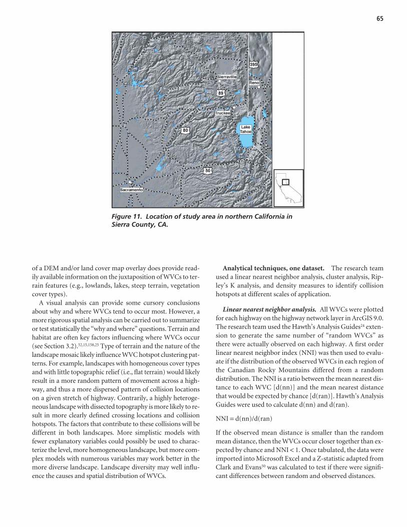
65

Figure 11. Location of study area in northern California inSierra County, CA.

of a DEM and/or land cover map overlay does provide read-ily available information on the juxtaposition of WVCs to ter-rain features (e.g., lowlands, lakes, steep terrain, vegetationcover types).

A visual analysis can provide some cursory conclusionsabout why and where WVCs tend to occur most. However, amore rigorous spatial analysis can be carried out to summarizeor test statistically the “why and where” questions. Terrain andhabitat are often key factors influencing where WVCs occur(see Section 3.2).52,15,158,25 Type of terrain and the nature of thelandscape mosaic likely influence WVC hotspot clustering pat-terns. For example, landscapes with homogeneous cover typesand with little topographic relief (i.e., flat terrain) would likelyresult in a more random pattern of movement across a high-way, and thus a more dispersed pattern of collision locationson a given stretch of highway. Contrarily, a highly heteroge-neous landscape with dissected topography is more likely to re-sult in more clearly defined crossing locations and collisionhotspots. The factors that contribute to these collisions will bedifferent in both landscapes. More simplistic models withfewer explanatory variables could possibly be used to charac-terize the level, more homogeneous landscape, but more com-plex models with numerous variables may work better in themore diverse landscape. Landscape diversity may well influ-ence the causes and spatial distribution of WVCs.

Analytical techniques, one dataset. The research teamused a linear nearest neighbor analysis, cluster analysis, Rip-ley’s K analysis, and density measures to identify collisionhotspots at different scales of application.

Linear nearest neighbor analysis. All WVCs were plottedfor each highway on the highway network layer in ArcGIS 9.0.The research team used the Hawth’s Analysis Guides24 exten-sion to generate the same number of “random WVCs” asthere were actually observed on each highway. A first orderlinear nearest neighbor index (NNI) was then used to evalu-ate if the distribution of the observed WVCs in each region ofthe Canadian Rocky Mountains differed from a randomdistribution. The NNI is a ratio between the mean nearest dis-tance to each WVC [d(nn)] and the mean nearest distancethat would be expected by chance [d(ran)]. Hawth’s AnalysisGuides were used to calculate d(nn) and d(ran).

NNI = d(nn)/d(ran)

If the observed mean distance is smaller than the randommean distance, then the WVCs occur closer together than ex-pected by chance and NNI < 1. Once tabulated, the data wereimported into Microsoft Excel and a Z-statistic adapted fromClark and Evans50 was calculated to test if there were signifi-cant differences between random and observed distances.

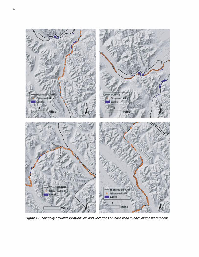
66

Figure 12. Spatially accurate locations of WVC locations on each road in each of the watersheds.

67

Region No.clusters

Mean cluster length

± SD (km)

No.high-killzones

Mean high-kill zone aggregation length

± SD (km)

Clusteroverlap indexa

TCH-Yoho (YNP) 6 1.00 ± 0.32 7 2.80 ± 1.33 1.00 TCH-Banff (BNP) 6 0.92 ± 0.38 11 4.40 ± 3.98 0.64 TCH-Alberta (AB) 7 1.32 ± 0.14 12 3.84 ± 1.63 0.90 Hwy 40-Kananaskis 6 0.96 ± 0.42 13 4.16 ± 3.29 0.85 Hwy 93-Kootenay (KNP) 17 0.86 ± 0.39 19 3.49 ± 2.34 0.56 a (cluster lengthhigh kill zone /cluster length)

Table 27. Descriptive statistics of the nearest neighbor clusters and high-kill zone aggregations.

The nearest neighbor index showed clustering (NNI < 1)for all highway regions except for the TCH in Yoho, whichshowed evidence of dispersion (Table 27). The Z-statistic wassignificant (P < 0.05) for the TCH in Alberta and marginallysignificant (P = 0.066) for Highway 93 South. The NNI usedin this analysis is only an indicator of first order spatial ran-domness; a K-order nearest neighbor distance (e.g., second orthird order) would likely better describe the overall spatialdistribution of WVCs.145 Sample sizes were small on the TCHin Yoho and Banff, and on Highway 40 in Alberta (n < 100),making overall spatial distributions of WVCs in these regionsdifficult to describe.

The linear NNI is a quick and easy statistical test of spatialdistribution of WVCs to initially determine whether colli-sions are distributed randomly across a stretch of highway orlarger highway network (e.g., a DOT district or region). If thetest indicates WVC clustering (NNI < 1.0), then the subse-quent step would be to identify where the clusters occur usinga GIS-based spatial analysis. Some spatial analysis techniquesinclude cluster analyses using a GIS-based NNI,25 mappingroadkill densities using a “moving window” analysis,213 or aroad segment approach to mapping roadkill densities.89,136

One approach that has great promise and is user-friendly isthe CrimeStat program developed by Levine.146

Cluster analysis: nearest neighbor hierarchical technique.The research team used CrimeStat version III146 to determinethe location of high-kill zones or WVC hotspots within eachof the five highways of the Canadian Rocky Mountains studyarea. CrimeStat is a nearest neighbor hierarchical technique,which identified a series of points that are spatially close basedon a predefined set of criteria.146 The clustering is repeateduntil either all points (WVCs) are grouped into a single clus-ter or else the clustering criterion fails. A fixed threshold dis-tance (800 m) was used for the search radius to determine theinclusion of a WVC in a cluster. This threshold distance(800 m) is the same radius used in the mile-marker densityanalysis (see “Density measures: WVCs per mile segment”below). The criterion for the minimum number of pointsrequired to define a cluster was the mean number of WVCsper mile for each highway region, the same criterion used to

determine whether a 1-mi buffer was a high- or low-kill zone(see “Density measures: WVCs per mile segment” below). Aconvex hull was used as the cluster output; it draws a polygonaround the WVCs in the cluster. Because roadkills occur in aone dimensional plane, a line was drawn from the two outer-most points along the road within the convex hull for visualdisplay and to calculate the length of each WVC cluster.

The nearest neighbor CrimeStat analysis produced a totalof 42 WVC clusters along 41 km of highway in the study area(Figure 13). Compared to the simple visual analysis ofWVCs, the CrimeStat modeling technique effectivelyreduced the blurring of WVC hotspots on long stretches ofhighway. As mentioned earlier, simple plotting of WVC lo-cations tends to result in tight groupings of collision pointsthat often overlap with other WVC locations, making it achallenge to identify where the really high-risk collision areasactually occur. The location and number of WVC hotspotsgenerated by the CrimeStat technique are clearly defined andcan be identified with associated landscape or road-relatedfeatures in each highway area.

Ripley’s K analysis. Ripley’s K statistic describes the dis-persion of data over a range of spatial scales.200,67 Ripley’s Kstatistic was calculated for all WVC mortalities in eachregion. The research team used the K statistic as defined byLevine,145 but modified it for points distributed in onedimension (e.g., along a line or road network). The result-ing algorithm was coded in Avenue™ and run in ArcViewGIS.77 The algorithm counted the number of neighboringWVCs within a specified scale distance (t) of each WVC,and these counts were summed over all WVCs. The researchteam standardized the WVC totals by sample size (N) andhighway length (RL) to allow for comparison between eachhighway region. The process was repeated for incrementallylarger scale distances up to RL for all five highways. The Kstatistic (adapted from Levine and O’Driscoll)77,185 wasdefined as:

KRL

NI

2( ) ( )distance dobs ij

j

N

ii j

N

===

≠

∑∑11

68

Figure 13. Clusters or hotspots derived from CrimeStat III software on each road in eachof the watersheds in Alberta, Canada.

69

A) TCH in Yoho NP

-8

-6

-4

-2

0

2

4

6

0 10 20 30 40 50

B) TCH in Banff NP

-3

-2

-1

0

1

2

3

4

5

6

0 10 20 30 40

C) TCH in Alberta

-3

-2

-1

0

1

2

3

4

5

0 10 20 30

D) Highway 40 Alberta

-4-3-2-101234567

0 10 20 30 40 50

E) Highway 93 South Kootenay NP

-5

0

5

10

15

20

25

30

0 20 40 60 80 100 120

Scale Distance t (km)

Figure 14. Plotted values of L statistic for the Ripley’s K statistic ofWVCs from five highways in Canadian Rocky Mountain study area.Ordinate axis is L(distance) for all 5 graphs.

where dij is the distance from WVC i to WVC j and I(dij) is anindicator function that returns 1 if dij <_ distance and returns 0if otherwise.185 A distance increment of 280 m was used for allfive highway regions to allow for a minimum of 100 ds bins onthe shortest section of highway (i.e., the TCH in Alberta).

To assess the significance of K-values, the research team ran50 simulations of the above equation based on random distri-butions of points for each of the five categories. Figure 14displays the results as plots of L versus distance, where L is thedifference between the observed K-value and the mean of theK-values for the 50 simulations.185 Positive values of L indicatecrowding and negative values indicate dispersion. Figure 14also presents the 95% confidence limits, calculated as theupper or lower 95th percentile of the random simulationsminus the mean of the random simulations.185 The researchteam defined significant crowding as any value of L above theupper confidence limit and significant dispersion as any valueof L below the lower confidence limit.

The distribution of WVCs was heterogeneous and signif-icantly more clustered or dispersed than would be expectedby chance over a wide range of scales (P < 0.05, Figure 14).In all highway regions there was significant clustering ofWVCs and some significant dispersion. The TCH in Yohohad a small degree of clustering from 1 to 2 km at an inten-sity of 0.3 km, and significant dispersion at spatial scalesfrom 3 to 12 km and 18 to 45 km. This dispersion peakedat an intensity of 7 km. Neighbor K statistics are well suitedfor the description of one-dimensional spatial distribu-tions.200,104,192 The range of scales over which clusteringappears significant is dependent on the intensity of the dis-tribution of roadkills.52,192 Peaks in L(t) (i.e., the intensity ofclustering) occurred between km 4 and 5 for the TCH inAlberta and the TCH in Banff, which means there was anaverage of 4 to 5 extra neighbors within the scale distance of0 to 10 km on the TCH in Banff and 0 to 12 km on the TCHin Alberta. Both these aggregations can be seen in Figure 14.

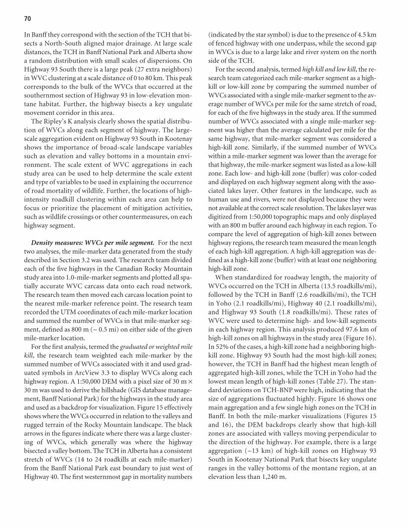
70

In Banff they correspond with the section of the TCH that bi-sects a North-South aligned major drainage. At large scaledistances, the TCH in Banff National Park and Alberta showa random distribution with small scales of dispersions. OnHighway 93 South there is a large peak (27 extra neighbors)in WVC clustering at a scale distance of 0 to 80 km. This peakcorresponds to the bulk of the WVCs that occurred at thesouthernmost section of Highway 93 in low-elevation mon-tane habitat. Further, the highway bisects a key ungulatemovement corridor in this area.

The Ripley’s K analysis clearly shows the spatial distribu-tion of WVCs along each segment of highway. The large-scale aggregation evident on Highway 93 South in Kootenayshows the importance of broad-scale landscape variablessuch as elevation and valley bottoms in a mountain envi-ronment. The scale extent of WVC aggregations in eachstudy area can be used to help determine the scale extentand type of variables to be used in explaining the occurrenceof road mortality of wildlife. Further, the locations of high-intensity roadkill clustering within each area can help tofocus or prioritize the placement of mitigation activities,such as wildlife crossings or other countermeasures, on eachhighway segment.

Density measures: WVCs per mile segment. For the nexttwo analyses, the mile-marker data generated from the studydescribed in Section 3.2 was used. The research team dividedeach of the five highways in the Canadian Rocky Mountainstudy area into 1.0-mile-marker segments and plotted all spa-tially accurate WVC carcass data onto each road network.The research team then moved each carcass location point tothe nearest mile-marker reference point. The research teamrecorded the UTM coordinates of each mile-marker locationand summed the number of WVCs in that mile-marker seg-ment, defined as 800 m (~ 0.5 mi) on either side of the givenmile-marker location.

For the first analysis, termed the graduated or weighted milekill, the research team weighted each mile-marker by thesummed number of WVCs associated with it and used grad-uated symbols in ArcView 3.3 to display WVCs along eachhighway region. A 1:50,000 DEM with a pixel size of 30 m ×30 m was used to derive the hillshade (GIS database manage-ment, Banff National Park) for the highways in the study areaand used as a backdrop for visualization. Figure 15 effectivelyshows where the WVCs occurred in relation to the valleys andrugged terrain of the Rocky Mountain landscape. The blackarrows in the figures indicate where there was a large cluster-ing of WVCs, which generally was where the highwaybisected a valley bottom. The TCH in Alberta has a consistentstretch of WVCs (14 to 24 roadkills at each mile-marker)from the Banff National Park east boundary to just west ofHighway 40. The first westernmost gap in mortality numbers

(indicated by the star symbol) is due to the presence of 4.5 kmof fenced highway with one underpass, while the second gapin WVCs is due to a large lake and river system on the northside of the TCH.

For the second analysis, termed high kill and low kill, the re-search team categorized each mile-marker segment as a high-kill or low-kill zone by comparing the summed number ofWVCs associated with a single mile-marker segment to the av-erage number of WVCs per mile for the same stretch of road,for each of the five highways in the study area. If the summednumber of WVCs associated with a single mile-marker seg-ment was higher than the average calculated per mile for thesame highway, that mile-marker segment was considered ahigh-kill zone. Similarly, if the summed number of WVCswithin a mile-marker segment was lower than the average forthat highway, the mile-marker segment was listed as a low-killzone. Each low- and high-kill zone (buffer) was color-codedand displayed on each highway segment along with the asso-ciated lakes layer. Other features in the landscape, such ashuman use and rivers, were not displayed because they werenot available at the correct scale resolution. The lakes layer wasdigitized from 1:50,000 topographic maps and only displayedwith an 800 m buffer around each highway in each region. Tocompare the level of aggregation of high-kill zones betweenhighway regions, the research team measured the mean lengthof each high-kill aggregation. A high-kill aggregation was de-fined as a high-kill zone (buffer) with at least one neighboringhigh-kill zone.

When standardized for roadway length, the majority ofWVCs occurred on the TCH in Alberta (13.5 roadkills/mi),followed by the TCH in Banff (2.6 roadkills/mi), the TCHin Yoho (2.1 roadkills/mi), Highway 40 (2.1 roadkills/mi),and Highway 93 South (1.8 roadkills/mi). These rates ofWVC were used to determine high- and low-kill segmentsin each highway region. This analysis produced 97.6 km ofhigh-kill zones on all highways in the study area (Figure 16).In 52% of the cases, a high-kill zone had a neighboring high-kill zone. Highway 93 South had the most high-kill zones;however, the TCH in Banff had the highest mean length ofaggregated high-kill zones, while the TCH in Yoho had thelowest mean length of high-kill zones (Table 27). The stan-dard deviations on TCH-BNP were high, indicating that thesize of aggregations fluctuated highly. Figure 16 shows onemain aggregation and a few single high zones on the TCH inBanff. In both the mile-marker visualizations (Figures 15and 16), the DEM backdrops clearly show that high-killzones are associated with valleys moving perpendicular tothe direction of the highway. For example, there is a largeaggregation (~13 km) of high-kill zones on Highway 93South in Kootenay National Park that bisects key ungulateranges in the valley bottoms of the montane region, at anelevation less than 1,240 m.

71

Figure 15. Weighted mile-markers derived from summed collisions by mile-marker on eachroad in each of the watersheds.

Comparison of Hotspot Identification Techniques

Visual analysis and observation versus analyticaltechniques. The pros and cons of the simple visual analysisof WVC versus more complex or analytical methods werediscussed earlier (“Simple graphic techniques, one dataset”).Essentially, with simple plotting of WVCs there is a tendency

for roadkill points to overlap and visually mask the impor-tance of segments of highway that have a high density ofWVCs. Modeling or analytical techniques permit a more de-tailed assessment of where WVCs occur, their intensity, andthe means to begin prioritizing highway segments for poten-tial mitigation applications. Last, the identification and de-lineation of WVC clusters, which often vary widely in length

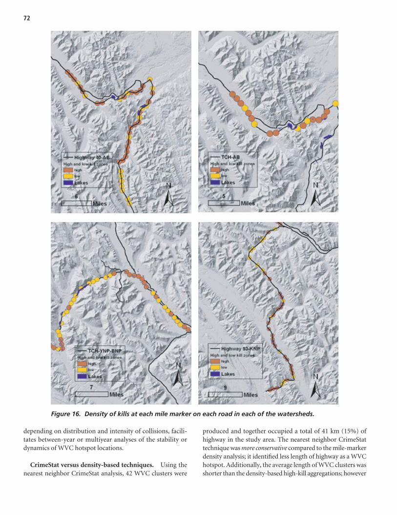
72

Figure 16. Density of kills at each mile marker on each road in each of the watersheds.

depending on distribution and intensity of collisions, facili-tates between-year or multiyear analyses of the stability ordynamics of WVC hotspot locations.

CrimeStat versus density-based techniques. Using thenearest neighbor CrimeStat analysis, 42 WVC clusters were

produced and together occupied a total of 41 km (15%) ofhighway in the study area. The nearest neighbor CrimeStattechnique was more conservative compared to the mile-markerdensity analysis; it identified less length of highway as a WVChotspot. Additionally, the average length of WVC clusters wasshorter than the density-based high-kill aggregations; however

73

Figure 17. Spatially accurate locations ofcarcasses from deer–vehicle collisions onState Route 89 in Sierra County, California.

the CrimeStat analysis produced clusters that were not con-tinuous (Table 27). If the research team had selected a largersearch radius for inclusion of roadkill points, fewer clusterswould have been identified. CrimeStat also consistently pro-duced fewer clusters of WVCs than the mile-marker densityanalysis.

Use of either technique for identifying WVC or roadkillhotspots may depend on the management objective. TheCrimeStat approach is useful for identifying key hotspot areason highways with many roadkills because it filters the road-kill data to extract where the most problematic areas lay. Themile-marker density analysis results in identifying morehotspot clusters on longer sections of highway. Although thisapproach appears to be less useful to management, it may bea preferred option where managers are interested in taking abroader, more comprehensive view of wildlife–vehicle con-flicts within a given area. This broader view may be necessarynot only to prioritize areas of conflicts but also to plan a suiteof mitigation measures. The location of the larger clustersproduced by the density analysis could be tracked each yearto determine how stable they are or whether there is a notableamount of shifting between years or over longer time periods.This type of information will be of value to managers in ad-dressing the type of mitigation and intended duration (e.g.,short-term vs. long-term applications).

The nearest neighbor CrimeStat clusters followed a spatialdistribution similar to the mile-marker high-kill zones (Fig-ure 13). The degree of overlap between the two techniqueswas high for three of the five highways. For example all theclusters on the TCH in Yoho fell within high-kill zone aggre-gations (Table 27). Similar patterns of overlap were found forthe TCH in Alberta and Highway 40 in Kananaskis Country.Less overlap of clusters defined by the two techniques wasfound for Highway 93 South and the TCH in Banff. Theseresults pose the questions: What mechanisms influence thespatial patterns of clusters derived by both techniques? Whyis cluster overlap high in some areas, but low in others? Bothtechniques coincided perfectly on the TCH in Yoho (100%overlap), whereas they were most divergent on Highway 93South in Kootenay National Park (roughly 50% overlap). Theoverlap of clusters on the other three highways was alignedwith either one of the two endpoints above. From inspectionof the WVC data on all five highways, the research teamsuggests that the amount of WVC cluster overlap from thetwo techniques is likely influenced by the density and distri-bution pattern of WVCs. High overlap was found on theTCH inYoho, where steep terrain dictates more or less whereanimals can cross the highway. There are few suitable loca-tions where wildlife can cross the TCH; thus, roadkills occurin clearly defined sections. Clusters will naturally overlap orbe in proximity because collisions rarely occur outside the keyhighway crossing areas. On highways that have less topo-graphic constraints and more dispersed wildlife habitat,

WVCs will tend to be greater in number and more uniformlydistributed than on the Yoho highway. Cluster definition willtend to diverge, and clusters from the two approaches will be-come spatially isolated. The reason is that the density-basedmethod has a tendency to accommodate outlying or marginalWVCs that normally would not cluster using CrimeStat.

Hotspot Identification and Patterns for Different Species and Landscapes

For this analysis, the research team selected one clusteringtechnique (CrimeStat) and conducted a hotspot analysis fortwo different datasets: WVC carcass data from CanadianRocky Mountains and Caltrans DVC carcass data for North-ern California. The data for Northern California wasdescribed previously in the “Study Area” section and shownin Figure 17. CrimeStat version III 146 was used to determinethe location of DVC carcass hotspots along SR 89 in SierraCounty, California, and the five highways in the CanadianRocky Mountains. For visual comparisons, the research teamplotted all DVC data along SR 89 in Sierra County, Califor-nia. The following paragraphs describe the hotspot patternsand configurations, and examine how they may differ byspecies and the two landscape types.

The mean number of DVCs along California SR 89 was25.7 kills/mi for the 26-year period and equates to roughly 1kill recorded per mile per year. The simple plotting of carcass

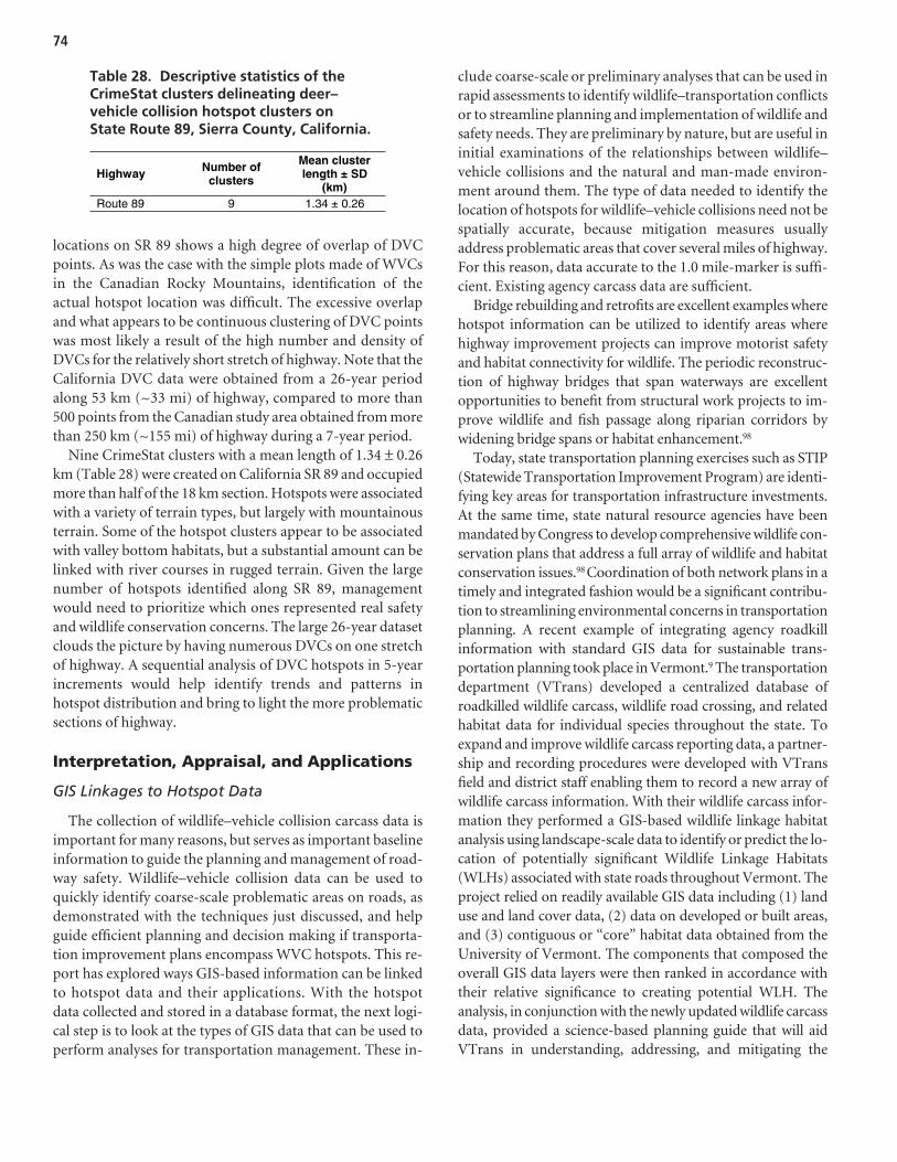
74

Highway Number of clusters

Mean cluster length ± SD

(km) Route 89 9 1.34 ± 0.26

Table 28. Descriptive statistics of theCrimeStat clusters delineating deer–vehicle collision hotspot clusters on State Route 89, Sierra County, California.

locations on SR 89 shows a high degree of overlap of DVCpoints. As was the case with the simple plots made of WVCsin the Canadian Rocky Mountains, identification of theactual hotspot location was difficult. The excessive overlapand what appears to be continuous clustering of DVC pointswas most likely a result of the high number and density ofDVCs for the relatively short stretch of highway. Note that theCalifornia DVC data were obtained from a 26-year periodalong 53 km (~33 mi) of highway, compared to more than500 points from the Canadian study area obtained from morethan 250 km (~155 mi) of highway during a 7-year period.

Nine CrimeStat clusters with a mean length of 1.34 ± 0.26km (Table 28) were created on California SR 89 and occupiedmore than half of the 18 km section. Hotspots were associatedwith a variety of terrain types, but largely with mountainousterrain. Some of the hotspot clusters appear to be associatedwith valley bottom habitats, but a substantial amount can belinked with river courses in rugged terrain. Given the largenumber of hotspots identified along SR 89, managementwould need to prioritize which ones represented real safetyand wildlife conservation concerns. The large 26-year datasetclouds the picture by having numerous DVCs on one stretchof highway. A sequential analysis of DVC hotspots in 5-yearincrements would help identify trends and patterns inhotspot distribution and bring to light the more problematicsections of highway.

Interpretation, Appraisal, and Applications

GIS Linkages to Hotspot Data

The collection of wildlife–vehicle collision carcass data isimportant for many reasons, but serves as important baselineinformation to guide the planning and management of road-way safety. Wildlife–vehicle collision data can be used toquickly identify coarse-scale problematic areas on roads, asdemonstrated with the techniques just discussed, and helpguide efficient planning and decision making if transporta-tion improvement plans encompass WVC hotspots. This re-port has explored ways GIS-based information can be linkedto hotspot data and their applications. With the hotspotdata collected and stored in a database format, the next logi-cal step is to look at the types of GIS data that can be used toperform analyses for transportation management. These in-

clude coarse-scale or preliminary analyses that can be used inrapid assessments to identify wildlife–transportation conflictsor to streamline planning and implementation of wildlife andsafety needs. They are preliminary by nature, but are useful ininitial examinations of the relationships between wildlife–vehicle collisions and the natural and man-made environ-ment around them. The type of data needed to identify thelocation of hotspots for wildlife–vehicle collisions need not bespatially accurate, because mitigation measures usuallyaddress problematic areas that cover several miles of highway.For this reason, data accurate to the 1.0 mile-marker is suffi-cient. Existing agency carcass data are sufficient.

Bridge rebuilding and retrofits are excellent examples wherehotspot information can be utilized to identify areas wherehighway improvement projects can improve motorist safetyand habitat connectivity for wildlife. The periodic reconstruc-tion of highway bridges that span waterways are excellentopportunities to benefit from structural work projects to im-prove wildlife and fish passage along riparian corridors bywidening bridge spans or habitat enhancement.98

Today, state transportation planning exercises such as STIP(Statewide Transportation Improvement Program) are identi-fying key areas for transportation infrastructure investments.At the same time, state natural resource agencies have beenmandated by Congress to develop comprehensive wildlife con-servation plans that address a full array of wildlife and habitatconservation issues.98 Coordination of both network plans in atimely and integrated fashion would be a significant contribu-tion to streamlining environmental concerns in transportationplanning. A recent example of integrating agency roadkillinformation with standard GIS data for sustainable trans-portation planning took place in Vermont.9 The transportationdepartment (VTrans) developed a centralized database ofroadkilled wildlife carcass, wildlife road crossing, and relatedhabitat data for individual species throughout the state. Toexpand and improve wildlife carcass reporting data, a partner-ship and recording procedures were developed with VTransfield and district staff enabling them to record a new array ofwildlife carcass information. With their wildlife carcass infor-mation they performed a GIS-based wildlife linkage habitatanalysis using landscape-scale data to identify or predict the lo-cation of potentially significant Wildlife Linkage Habitats(WLHs) associated with state roads throughout Vermont. Theproject relied on readily available GIS data including (1) landuse and land cover data, (2) data on developed or built areas,and (3) contiguous or “core” habitat data obtained from theUniversity of Vermont. The components that composed theoverall GIS data layers were then ranked in accordance withtheir relative significance to creating potential WLH. Theanalysis, in conjunction with the newly updated wildlife carcassdata, provided a science-based planning guide that will aidVTrans in understanding, addressing, and mitigating the

75

effects of roads on wildlife movement, mortality, and habitatand public safety early in the design process for transportationprojects.

There are a variety of GIS modeling approaches today, fromsimple to more complex models requiring high-resolutionand spatially explicit data. Most GIS modeling used for trans-portation planning purposes tends to be coarse scale and doesnot require specially developed GIS data layers.13,65,212 LikeGIS-based data on animal movements, hotspot informationcan be used to identify problematic areas and thus integratemitigation where highway improvement capital will beinvested. Hotspot areas that are associated with existingbelow-grade crossings (e.g., drainage culverts and bridges) canbe identified by linking GIS data, allowing structural and landplanning recommendations to be made to improve perme-ability at unsuitable passages.

In another example, WVC carcass data were used alongInterstate 90 in Washington to evaluate the relationship be-tween hotspot clusters and important landscape characteris-tics.214 Carcass density was mapped using the approachdescribed earlier, classifying segments as high, moderate, or lowungulate-kill density. A classification tree analysis (using S-Plus2000) was used to determine the importance of 10 landscape-scale variables (GIS layers comprising road and landscape fea-tures) in the study area. Classification tree analysis is well suitedfor analysis of GIS spatial data. Being a non-parametric tech-nique, it involves no assumptions of normal distribution, workswell with categorical data, and is robust to the relatively subjec-tively determined sample sizes inherent with GIS raster data.Further, linking these coarse-scale hotspots with environmen-tal data (e.g., terrain, habitat suitability, zones of animal move-ment) can provide a relatively quick and reliable project-levelor district-level assessment of how to prioritize mitigationactivities directed at wildlife–vehicle collisions.

Conclusions

In this section the research team suggests guidelines forhotspot application. Data on hotspots of WVCs can helptransportation managers increase motorist safety and habitatconnectivity for wildlife by providing safe passage for wildlifeacross busy roadways. Knowledge of the geographic locationand severity of WVCs is a prerequisite for devising mitigationschemes that can be incorporated into future infrastructureprojects such as bridge reconstruction and highway expan-sion. Hotspots in proximity to existing below-grade wildlifepassages can help inform construction of structural retrofitsthat can help keep wildlife off roadways and increase habitatconnectivity.

The WVC data that transportation departments currentlypossess are suitable for meeting the primary objective ofidentifying hotspot locations at a range of geographic scales,

from project-level (< 50 km of highway) to larger district-level or state-wide assessments on larger highway networksystems. The spatial accuracy of WVCs is not of criticalimportance for the relatively coarse-scale analysis of wherehotspots are located. To determine site-specific factors thatcontribute to WVCs, more spatially accurate data arerequired. Thus, WVCs referenced to a mile-marker systemwill be sufficient for transportation agencies to identify thelocation of problematic areas for motorists and wildlife.WVC data with greater spatial accuracy are equally useful indetermining the location of hotspots; however, they are notessential to begin examining highway–wildlife conflict areas.

The research team has outlined and described various tech-niques available that can help delineate WVC hotspots. Sim-ple plotting of collision points is a relatively straightforwardmeans of identifying problematic areas; however, as samplesizes increase, the tendency for roadkilled carcasses to overlap(hide other points) increases. The length of highway exam-ined, the number of animals killed, and time period of datacollection all influence the density of collision points. Otherfactors such as terrain, wildlife abundance, and wildlife habitatquality adjacent to the highway will further affect the spatialdistribution (random/continuous or non-random/clustered)of WVCs on a given highway. Modeling or analytical tech-niques permit a more rigorous assessment of where WVCs arelikely to occur, their intensity, and the means to begin priori-tizing highway sections for mitigative actions. The nearestneighbor CrimeStat method essentially pinpoints the locationof WVC hotspots, whereby the segmental analyses of WVCdensities provide a more comprehensive evaluation of mitiga-tion options and prioritization of mitigation schemes basedon cost-benefit, scheduling of transportation projects, orseverity of motorist safety concerns.

Collection of WVC data (both reported vehicle collisionand carcass collection data) by transportation departmentswill be increasingly beneficial, especially if the collectionprocedures are more systematic. Currently, in many stateagencies, WVC data collection is not consistent and variesfrom district to district. The research team is not aware ofmany state transportation departments that have consis-tently used WVC hotspot data for decision making intransportation projects or strategic planning with futureinfrastructure plans such as STIP in mind. Systematic datacollection and protocols will allow for cost-effective use ofthe data and greater management benefits by providingimportant baseline information for planning environmen-tal mitigation in projects. Further, properly collectedpre-mitigation data provide a critical reference point forultimately assessing the performance of mitigation meas-ures that are adopted.

See Appendix E for a literature review of papers that haveaddressed hotspot identification.

76

3.4 Influence of Roads on Small Mammals

Introduction

Highways have the potential to affect the abundance anddistribution of small mammals. Differences in the density ofmany small mammals have been reported when road vergeshave been compared to the habitats beyond them.2,1,19 Thisdensity difference may be due to structural or vegetative dif-ferences in habitat, water runoff, or the additional impact ofnoise, vibration, deposition of road salt or other chemicals, ordifferential rates of predation between the verge and adjacentland. Highways may also act as barriers or partial barriers tomovement.186,143,153,103,49,107,170,36 Such barriers may indirectlylead to population impacts due to the reduced probability ofgenetic flow and demographic “rescue” (inflow of animals tocounter local extirpations caused by random events) for smallpopulations. Direct mortality of small mammals on the high-way surface186 appears to have variable effects on populationdensity2 as well as demographic changes such as the dispro-portionate loss of sex or age classes that tend to disperse.While highways have been well established as contributing tosuch impacts,186,143,153,103,49,107,170,36 to what extent is not entirelyclear. Questions remain as to what impact highways, includ-ing traffic volume, have on the diversity and density of speciesfound in the dry forested ecosystems typical of much of themountainous region of western North America, to what ex-tent the effects extend beyond the highway, and if the impactsare due to the highway specifically or to the presence of a dis-turbed ROW generally.

Both direct effects (animal mortality) and indirect effectsinfluence animal response to the roaded landscape. Direct ef-fects such as actual road kills, impact all species, but collisionswith larger wildlife species (deer, elk, moose, caribou, andlarge carnivores) pose the most risk to driver safety and resultin higher automobile damage and human injury. Knapp(www.deercrash.com/states/data.htm) showed that for thefive-state Upper Midwest (Illinois, Iowa, Michigan, Wisconsin,and Minnesota), 121,584 deer-vehicle collisions caused over$206.6 million in vehicle damages, but more important, re-sulted in 35 human deaths and 4,666 injuries from 2003 to2004. Direct effects are on the rise, and so are the costs to cit-izens. Indirect effects of roads on wildlife putatively are as im-portant to ecological communities as are direct effects such asmortality. The most commonly reported indirect effects in-clude (1) loss of habitat, (2) reduction of habitat quality, (3)fragmentation of once “more continuous” habitat with asso-ciated increases in edge density and edge buffer effects, (4)habitat disconnectedness, and (5) barrier effects. One com-plication is that the landscape consequences from indirecteffects are interrelated suggesting that parsing out the contri-bution of each effect will take a long-term experimental

approach. Such an approach is not possible or feasible in thetime available for this project. However, permeability can beassessed and species responses to roaded landscapes can bemeasured. The null hypothesis that the research team testedis that indirect effects, taken as a whole, have little significanteffect on animal population response. Significant was definedas greater than 10% deviation, after background variation hasbeen taken into account. The first level predicted responseswere an expected species’ presence or absence, composition,and relative abundance to change at increasing distancesfrom the road if habitat quality was reduced, if habitat frag-mentation was increased, if there were edge buffer effects, ifthere was habitat disconnectedness, and if there were barriereffects.

Assessment of causality to a specific indirect effect was notpossible or practical within the time schedule and fundingavailable. The summation of the effects, however, was simpleto document. Animal response near roads could be comparedwith a control response to a non-roaded area. The term “re-sponse” means the difference in the number of small mam-mal species diversity and their relative abundance. Jaeger et al.133 explained that roads and traffic can affect the persis-tence of animal populations in four distinct ways: (1) a de-crease in habitat amount and quality, (2) increased mortal-ity, (3) barrier effects that prevent animals from accessingresources across the road, resulting in (4) fragmented andsubdivided populations.

The small-mammal research in Utah and British Colum-bia allowed the impact of roads on habitat quality for smallmammals to be assessed at varying distances from the road.If habitat quality declined due to road traffic, the researchteam expected a decline in the numbers and relative abun-dance of small-mammal species nearer to roads. To investi-gate this question, the research team compared the relativeabundance of small mammals at varying distances from amajor interstate highway in Utah and a two-lane highway andhigh-voltage transmission-line ROW in British Columbia.These locations allowed the research team to compare the ef-fects of two very different types of roads while simultaneouslyaddressing the effect of distance from the ROWs.

For this field effort, the research team selected sites in west-ern British Columbia and in the Intermountain Region ofUtah to determine if any general response of small, terrestrialvertebrates exists for arid and mesic sites. There is tremen-dous variation across the North American continent in termsof vegetation cover, topography, levels of urban develop-ment, land use practices, road density, and traffic volume, aswell as differences in the typical species diversity, richness,and abundance in local areas. Yet, it was impossible to cap-ture that entire variation in one study. Nevertheless, this isthe case with most ecological studies, and there is an impera-tive to capture the basic ecological responses and apply those

77

fundamental principles to mitigation and management. Theapproach for this study was to develop ecological principlesthat have conceptual generality and that can be appliedbroadly. The caveat of course is the necessity for gatheringlocal, empirical data that will inform the programming, plan-ning, design, and construction phases of building, upgrading,and maintaining roads.

For this effort, sites characterized by natural vegetationlocated next to roads were selected and compared to sitesdistant from the road. Indirect effects have been suggested tooperate within 100 m of a road; however, as a precaution, wedesigned our sampling protocol to detect changes that mayoccur up to 600 m or more from the road. Small mammalshave relatively small home ranges and limited mobility, andthe research team expected that results should be evidentwithin 600 m from the road. The research team measuredsmall-mammal species’ presence or absence, composition,and relative abundance through trapping periods in the sum-mer months of 2004 and 2005.

In both Utah and British Columbia, the research teamsampled at increasing distances from the road to addressthese putative effects:

• If habitat quality is reduced near the roadway, the presenceor absence, composition, and relative abundance of speciesis expected to change at increasing distances from the road.

• If there are edge buffer effects along the road, there is ex-pected to be a zone close to the road where the presence,abundance, and composition of species will be dramati-cally influenced.

Research Approach: Methods and Data

The work for this segment was conducted in Utah andBritish Columbia in two very different habitats. Utah is lo-cated in the Intermountain West of the United States. Thestudy site was composed mainly of sagebrush (Artemisia spp.)habitat, and the road verge (ROW) is largely non-vegetated.Conversely, the British Columbia site in Canada is heavilyforested with a densely vegetated road verge. The researchteam adapted its sampling scheme to maximize capture ofsmall mammals for these very different sites. The followingparagraphs describe how the field work was conducted ineach site. The research team began work in Utah in 2004 aspart of an ongoing study and continued in 2005. In BritishColumbia, the research team conducted the field work dur-ing summer 2005.

Utah

Permeability and small-mammal trapping. This studywas conducted in the high-elevation desert region of the

Great Basin of western Utah near Beaver, Utah (latitude38°16′ N and longitude 112°37′ W), adjacent to Interstate 15(I-15), a four-lane divided highway with an average of 16,015vehicles/day. Elevation ranged from 1,700 to 1,900 m (5,500to 6,300 ft). Vegetation cover was dominated by big sage-brush (Artemisia tridentata) with an occasional inclusionof pinyon pine (Pinus edulis) and juniper (Juniperusosteosperma) trees. The road verge included sagebrush andgrassy vegetation or was completely non-vegetated. Theweather was characterized by below-freezing temperaturesand snow cover during the winter and high temperaturesduring the summer. Maximum temperatures occasionallyexceeded 38°C (100°F) and minimum temperatures wereusually above –23°C (–10°F), with annual mean temperatureof 8.6°C (47.4°F). Annual precipitation (in the form of rainand snow) was less than 305 mm (12 in.), and came prima-rily during winter, early spring, and late summer. Relativehumidity was very low and evaporation potential was high.Prolonged periods of drought are frequent in the region. Thesoil on the trapping sites was composed mainly of fine sanddeposits with occasional volcanic rocky areas. Study siteswere established in sagebrush-steppe vegetation along 20 mi(~32.2 km) of Interstate 15, centered on UTM (NAD27) X =354471 Y = 4248267. Small-mammal sampling was con-ducted exclusively in sagebrush habitat on both sides of theroad (Figure 18). Because changes in sagebrush habitat weredetected along the road, the research team designated the dif-fering habitats A, B, and C.

Small mammals were live and lethal trapped from 30 Mayto 14 August in 2004 and from 17 June to 18 August in 2005.The trapping design was altered between the 2004 and 2005field seasons to maximize the useful information gleaned. In2004, trapping webs were used to assess road influence onsmall-mammal communities. In 2005, the research team usedtrapping lines to compare the Utah results with the British Co-lumbia trapping scheme. During summer 2004, 12 transectswere completed with 2 trapping webs per transect, for a totalof 24 webs. The first trapping web was placed at 50 m (close)and the second at 400 m (distant) from the road (Figure 19).Each web was composed of eight segments extending 50 moutwards from a central point. Each segment had six trappingstations of two traps each, located 5, 10, 20, 30, 40, and 50 mfrom center, with one trapping station located at the center ofthe web for a total of 98 traps [half lethal (snap) and half live(non-lethal)] per web and a total of 2,352 traps for the 24webs. During summer 2005, 3 trapping lines were placed par-allel to the road along each of 5 transects (Figure 19) for a totalof 15 trapping lines. Lines were placed at increasing distancesfrom the exclusion fence: at 0 m (close), 200 m (mid), and600 m (distant). Each line was 150 m in length and contained30 traps total, for a total of 450 traps for the 15 trapping lines.The research team completed a total of 8,406 trap-nights. For

78

Figure 18. Sagebrush habitat in southwestern Utah where small-mammal trapping was conducted.

Close

Close Mid

Distant

Distant

2004

2005

Figure 19. Schematic representation of sampling schemes in 2004 and 2005.

safety reasons, the ROW verge between the road edge and the2.4 m deer exclusion fence was not sampled because of veryhigh traffic volume.

All traps in both sampling schemes were baited with a mix-ture of horse grain and peanut butter, and checked on threeconsecutive mornings and afternoons (lethal traps only).Upon capture, all animals were identified, sex determined,measured, marked, and released. Dead animals were removedfrom the study site.

Data analyses. Web-based data analysis for 2004 em-ployed a distance method described by Anderson et al.5 thatutilizes first capture locations for each individual and distanceto the center of the web plot. The software program Distance4.140,41 was used to calculate densities and variance estimates.

For analysis, capture data was pooled in “close webs” and “dis-tant webs” because of the low number of animals sampled ineach web. Estimation was only possible for the most abundantspecies (i.e., > 30 captured individuals per pooled database) orfor all small mammals combined. Density estimations in Dis-tance were obtained by every possible combination of models(uniform, half-normal, hazard, and negative exponential) andadjustment terms (cosine, simple polynomial, and Hermitepolynomial). See Appendix F. Final model selection was basedon Akaike’s Information Criterion (AIC) value and on modelperformance. Each dataset was used in its entirety withouttruncation. Intervals used in Distance (0.0, 7.5, 15, 25, 35, and45 m) were the midpoints between trap-stations. Resultingdensities in close and distant webs were tested for significantdifferences using Wald test.

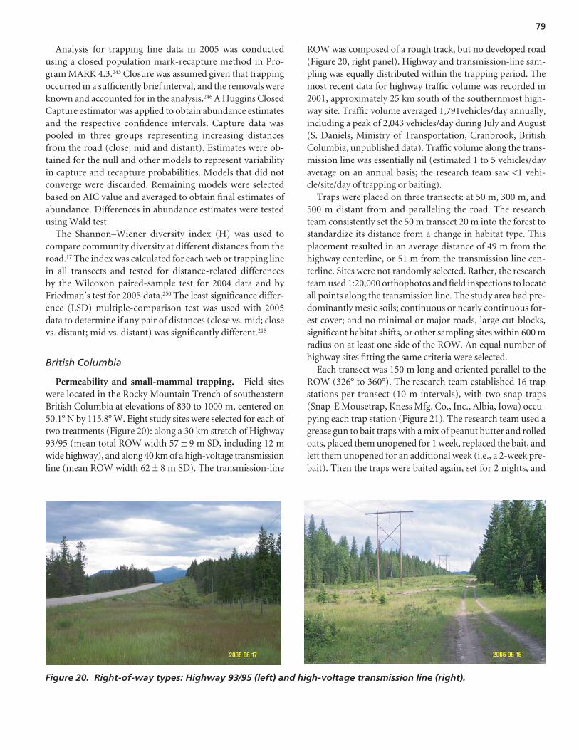
79

Analysis for trapping line data in 2005 was conductedusing a closed population mark-recapture method in Pro-gram MARK 4.3.243 Closure was assumed given that trappingoccurred in a sufficiently brief interval, and the removals wereknown and accounted for in the analysis.246 A Huggins ClosedCapture estimator was applied to obtain abundance estimatesand the respective confidence intervals. Capture data waspooled in three groups representing increasing distancesfrom the road (close, mid and distant). Estimates were ob-tained for the null and other models to represent variabilityin capture and recapture probabilities. Models that did notconverge were discarded. Remaining models were selectedbased on AIC value and averaged to obtain final estimates ofabundance. Differences in abundance estimates were testedusing Wald test.

The Shannon–Wiener diversity index (H) was used tocompare community diversity at different distances from theroad.17 The index was calculated for each web or trapping linein all transects and tested for distance-related differencesby the Wilcoxon paired-sample test for 2004 data and byFriedman’s test for 2005 data.250 The least significance differ-ence (LSD) multiple-comparison test was used with 2005data to determine if any pair of distances (close vs. mid; closevs. distant; mid vs. distant) was significantly different.218

British Columbia

Permeability and small-mammal trapping. Field siteswere located in the Rocky Mountain Trench of southeasternBritish Columbia at elevations of 830 to 1000 m, centered on50.1° N by 115.8° W. Eight study sites were selected for each oftwo treatments (Figure 20): along a 30 km stretch of Highway93/95 (mean total ROW width 57 ± 9 m SD, including 12 mwide highway), and along 40 km of a high-voltage transmissionline (mean ROW width 62 ± 8 m SD). The transmission-line

ROW was composed of a rough track, but no developed road(Figure 20, right panel). Highway and transmission-line sam-pling was equally distributed within the trapping period. Themost recent data for highway traffic volume was recorded in2001, approximately 25 km south of the southernmost high-way site. Traffic volume averaged 1,791vehicles/day annually,including a peak of 2,043 vehicles/day during July and August(S. Daniels, Ministry of Transportation, Cranbrook, BritishColumbia, unpublished data). Traffic volume along the trans-mission line was essentially nil (estimated 1 to 5 vehicles/dayaverage on an annual basis; the research team saw <1 vehi-cle/site/day of trapping or baiting).

Traps were placed on three transects: at 50 m, 300 m, and500 m distant from and paralleling the road. The researchteam consistently set the 50 m transect 20 m into the forest tostandardize its distance from a change in habitat type. Thisplacement resulted in an average distance of 49 m from thehighway centerline, or 51 m from the transmission line cen-terline. Sites were not randomly selected. Rather, the researchteam used 1:20,000 orthophotos and field inspections to locateall points along the transmission line. The study area had pre-dominantly mesic soils; continuous or nearly continuous for-est cover; and no minimal or major roads, large cut-blocks,significant habitat shifts, or other sampling sites within 600 mradius on at least one side of the ROW. An equal number ofhighway sites fitting the same criteria were selected.

Each transect was 150 m long and oriented parallel to theROW (326° to 360°). The research team established 16 trapstations per transect (10 m intervals), with two snap traps(Snap-E Mousetrap, Kness Mfg. Co., Inc., Albia, Iowa) occu-pying each trap station (Figure 21). The research team used agrease gun to bait traps with a mix of peanut butter and rolledoats, placed them unopened for 1 week, replaced the bait, andleft them unopened for an additional week (i.e., a 2-week pre-bait). Then the traps were baited again, set for 2 nights, and

Figure 20. Right-of-way types: Highway 93/95 (left) and high-voltage transmission line (right).

80

Figure 21. Schematic of site layout for a highway site.

checked each morning. Animals trapped were removed,tentatively identified to species and bagged, then positivelyidentified, sexed, weighed, and measured later on the day ofcapture. The research team completed all capture work from14 through 18 June and 4 through 8 July 2005.

The study site was within the Interior Douglas-Fir biogeo-climatic zone (IDF) in the province’s dry climatic region.35

Within the IDF, six “site series” (descriptors of potential cli-max vegetation and soil moisture) have been described. Theresearch team judged the forested portion of all sites to becomposed historically of the same predominant site series:Douglas-fir (Pseudotsuga menziesii), lodgepole pine, (Pinuscontorta), pinegrass (Calamogrostis rubescens), and twinflower(Linnaea borealis). However, because of topographic variabil-ity, past wildfires, and partial-cut logging, study sites weremid-seral mixes of Douglas-fir, lodgepole pine, western larch(Larix occidentalis), and ponderosa pine (P. ponderosa), witha minor component of trembling aspen (Populus tremuloides)and paper birch (Betula papyrifera). The research team did notmeasure habitat variables, but did record general habitat con-ditions subjectively. Crown closure was typically 40% to 60%,with portions of some sites ranging from about 10% to 80%.At all sites, the dominant understory plant was pinegrass withroughly 5% to 20% cover, but up to approximately 50% coverin some small openings of past disturbance. Other commonunderstory species in all sites included soopolallie (Shepherdiacanadensis), birch-leaved spirea (Spiraea betulifolia), commonsnowberry (Symphoricarpos albus), saskatoon (Amelanchieralnifolia), Douglas-fir saplings, and heart-leaved arnica (Ar-nica cordifolia). Tall Oregon grape (Mahonia aquifolium),showy aster (Aster conspicuus), twinflower, wild strawberry(Fragaria virginiana), and a variety of mosses contributed to

the greater ground cover in moister microhabitats or coolaspects. Bluebunch wheatgrass (Agropyron spicatum), june-grass (Koeleria macrantha), arrow-leaved balsamroot (Bal-samorhiza sagittata), and kinnikinnick (Arctostaphylos uva-ursi) were more commonly present in drier locations with asparse understory and less pinegrass. Small patches underdense Douglas-fir cover had essentially no understory. Whiledowned woody debris was sporadically present, there was typ-ically little of this because of the relatively young forest age andits history of past disturbance. All ROWs were predominantlyvegetated by wild and/or agronomic grasses and wild straw-berry, with variable cover of other forbs, no trees or downedwoody debris, and minimal shrub cover.

Data analyses. The research team compared the numberof species trapped (and abundance of each) among transectsand among treatments. Where sample sizes permitted, the re-search team also compared weights of adult males, weights ofadult females, sex ratios and juvenile:adult ratios among tran-sects and treatments using t-tests and χ2 tests as appropriateusing the program JMP IN (SAS Institute, Inc., Cary, NorthCarolina).

Findings and Results

Utah

In 2004, a total of 11 species were captured; two specieswere captured exclusively in areas close to the road (rocksquirrel [Spermophilus variegates] and sagebrush vole [Lem-miscus curtatus]), and two species were captured exclusivelydistant from the road (piñon mouse [Peromyscus truei] and

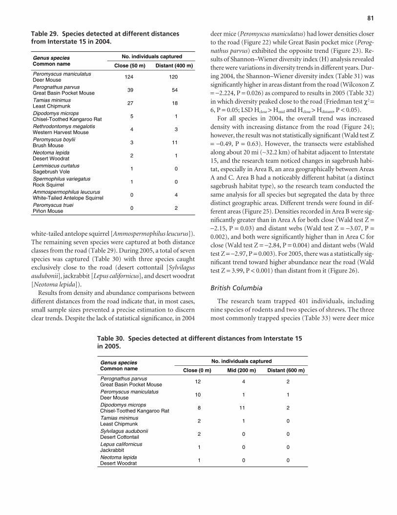
81

No. individuals captured Genus speciesCommon name Close (50 m) Distant (400 m)

Peromyscus maniculatusDeer Mouse 124 120

Perognathus parvus Great Basin Pocket Mouse 39 54

Tamias minimusLeast Chipmunk 27 18

Dipodomys micropsChisel-Toothed Kangaroo Rat 5 1

Rethrodontomys megalotis Western Harvest Mouse 4 3

Peromyscus boyliiBrush Mouse 3 11

Neotoma lepidaDesert Woodrat 2 1

Lemmiscus curtatusSagebrush Vole 1 0

Spermophilus variegatus Rock Squirrel 1 0

Ammospermophilus leucurusWhite-Tailed Antelope Squirrel 0 4

Peromyscus truei Piñon Mouse 0 2

Table 29. Species detected at different distancesfrom Interstate 15 in 2004.

No. individuals captured Genus speciesCommon name Close (0 m) Mid (200 m) Distant (600 m)

Perognathus parvus Great Basin Pocket Mouse 12 4 2

Peromyscus maniculatusDeer Mouse 10 1 1

Dipodomys micropsChisel-Toothed Kangaroo Rat 8 11 2

Tamias minimusLeast Chipmunk 2 1 0

Sylvilagus auduboniiDesert Cottontail 2 0 0

Lepus californicus Jackrabbit 1 0 0

0 Neotoma lepidaDesert Woodrat 1 0

Table 30. Species detected at different distances from Interstate 15in 2005.

white-tailed antelope squirrel [Ammospermophilus leucurus]).The remaining seven species were captured at both distanceclasses from the road (Table 29). During 2005, a total of sevenspecies was captured (Table 30) with three species caughtexclusively close to the road (desert cottontail [Sylvilagusaudubonii], jackrabbit [Lepus californicus], and desert woodrat[Neotoma lepida]).

Results from density and abundance comparisons betweendifferent distances from the road indicate that, in most cases,small sample sizes prevented a precise estimation to discernclear trends. Despite the lack of statistical significance, in 2004

deer mice (Peromyscus maniculatus) had lower densities closerto the road (Figure 22) while Great Basin pocket mice (Perog-nathus parvus) exhibited the opposite trend (Figure 23). Re-sults of Shannon–Wiener diversity index (H) analysis revealedthere were variations in diversity trends in different years. Dur-ing 2004, the Shannon–Wiener diversity index (Table 31) wassignificantly higher in areas distant from the road (Wilcoxon Z= −2.224, P = 0.026) as compared to results in 2005 (Table 32)in which diversity peaked close to the road (Friedman test χ2 =6, P = 0.05; LSD Hclose > Hmid and Hclose > Hdistant, P < 0.05).

For all species in 2004, the overall trend was increaseddensity with increasing distance from the road (Figure 24);however, the result was not statistically significant (Wald test Z= −0.49, P = 0.63). However, the transects were establishedalong about 20 mi (∼32.2 km) of habitat adjacent to Interstate15, and the research team noticed changes in sagebrush habi-tat, especially in Area B, an area geographically between AreasA and C. Area B had a noticeably different habitat (a distinctsagebrush habitat type), so the research team conducted thesame analysis for all species but segregated the data by threedistinct geographic areas. Different trends were found in dif-ferent areas (Figure 25). Densities recorded in Area B were sig-nificantly greater than in Area A for both close (Wald test Z =−2.15, P = 0.03) and distant webs (Wald test Z = −3.07, P =0.002), and both were significantly higher than in Area C forclose (Wald test Z = −2.84, P = 0.004) and distant webs (Waldtest Z = −2.97, P = 0.003). For 2005, there was a statistically sig-nificant trend toward higher abundance near the road (Waldtest Z = 3.99, P < 0.001) than distant from it (Figure 26).

British Columbia

The research team trapped 401 individuals, includingnine species of rodents and two species of shrews. The threemost commonly trapped species (Table 33) were deer mice

82

Diversity Index Transect

Hclose Hdistant

1 0 0 2 0.8 1.27 3 0.8 1.01 4 0 0.3 5 0.35 0.56 6 0.35 1.04 7 1.17 1.3 8 0.43 0.6 9 0.6 0.67 10 0 0.5 11 0.14 0 12 0.99 0.81

Table 31. Values of Shannon–Wiener diversityindex (H) estimated for 2004 by transect in closeand distant webs in Utah.

Diversity Index Transect

Hclose Hmid Hdistant

1 0.67 0.69 0

2 0.64 0 0

3 1.31 0 0.64

4 1.35 1 0

5 1.04 0.45 0

Table 32. Values of Shannon–Wiener diversity index (H) estimated for 2005 by transect in close, mid, and distant trapping lines in Utah.

Den

sity

Est

imat

es (

P. p

arvu

s)

close distant

Distance from Road

29.6

20.2

0

10

20

30

40

50

60

70

Figure 23. Density estimates of Perognathus parvusin 2004 at different distances from the road.

(Peromyscus maniculatus), southern red-backed voles(Clethrionomys gapperi), and yellow-pine chipmunks(Tamias amoenus). True trapping effort was slightly unevenamong treatments, sites, and transects because of varioustrapping impediments that are inherent to field work inwhich environmental variables are not always controllable

(Table 33). Trapping problems included several brief butheavy rains that snapped traps, larger animals stepping ontraps or otherwise snapping them, non-functional traps,usually due to soil thrown up by the impact of raindrops,and a few captures of songbirds which prevented the captureof small mammals. As a result, realized trapping effort was78% of attempted trapping effort. Capture rates, adjustedfor realized trapping effort (Table 33), were low and un-evenly distributed spatially for most species. Total capturerates were 9.8 and 12.6 captures per 100 trap-nights, in re-lation to attempted and realized trapping effort respectively.Six species were more abundant at highway sites, while fivewere more abundant at transmission-line sites. Five specieswere present at more highway than transmission-line sitesand four were present at more transmission-line than high-way sites. The low sample sizes and clumpy, among-site dis-tribution of captures prevented within-species comparisonsof spatial distribution in relation to transect, with the ex-ception of deer mice (Figure 27). For this species, there wasno difference in capture rate among transects for highwaysites (χ2 P = 0.93) but a difference was realized for trans-mission-line sites (P = 0.04). Comparing highway to trans-mission-line sites for each transect, a marginally significant

83.9

168.3

0

50

100

150

200

250

300

350

400

450

close distant

Distance from Road

Den

sity

Est

imat

es (

P. m

anic

ula

tus)

Figure 22. Density estimates of Peromyscus manicu-latus in 2004 at different distances from the road.

83

difference was evident for deer mice between treatmentsonly for the 600 m transect (ROW P = 0.32, 50m P = 0.47,300m P = 0.83, 600m P = 0.05).

For both male and female deer mice, animal weights didnot differ among transects for highway or transmission-linesites (ANOVA P > 0.44 for all comparisons; Figure 28). Com-paring highway to transmission-line sites for each sex andtransect, no differences in weight were evident (t-test P > 0.24for all comparisons) with the possible exception of males onthe 600 m transect (P = 0.06).

There was no difference in sex ratio among transects forhighway sites (χ2 P = 0.88), but there was some evidence of adifference among transects for transmission-line sites (P =0.07; Figure 29). Comparing highway to transmission-linesites for each transect, there was weak evidence of a differencebetween treatments only for the 600 m transect (ROW P =0.92, 50 m P = 0.79, 300 m P = 0.32, 600 m P = 0.09).

Juvenile:adult ratios did not vary significantly among tran-sects for either treatment, or among transect for any treatment

(χ2 P > 0.17 for all comparisons except highway vs. transmis-sion line for ROW transect, for which P = 0.08; Figure 30).Sample sizes were relatively low, likely due to a combinationof a low realized trapping effort, some periods of inclementweather that may have limited animal activity and survivor-ship, and the timing of sampling effort. The field season oc-curred in early June and July when recovery from the annualwinter population decline would have been incomplete forsome species.225 Combining all transects per site, similar pat-terns of diversity and abundance were evident between trans-mission-line and highway sites, although distribution wasclumpy for most species. With the exception of deer mice andyellow-pine chipmunks, each species occurred at fewer thanhalf of the sites, despite being common at some of those sites.For any given transect distance, only deer mice were trappedat more than half of the sites. This clumping suggests thatwithin the forest, microhabitat or some other localized effectwas stronger than any influence of distance to the highway.

Species diversity was lowest in ROW transects than anyother transect. However, there is no strong evidence to suggestthat this observation was related to anything beyond a shiftfrom native forest at 50, 300, and 600 m transects, to the lesscomplex structure and vegetation of the disturbed habitat inthe ROW. For example, optimal habitat for yellow-pine chip-munks appears to be open forest with abundant woody debris;southern red-backed voles are most common in matureforests with abundant shrub and ground cover; heather volesare associated with a dense shrub layer and abundant woodydebris; and in the dry interior of British Columbia where thisstudy area was located, long-tailed voles are associated withshrub thickets.178 Thus, ROWs with no forest or downedwoody debris and few shrubs would be expected to have fewerof these species, independent of the presence of a highwaynearby. The only species trapped more often on ROW tran-sects was the western jumping mouse, consistent with its

0

50

100

150

200

250

300

350

close distant

Distance from Road

Den

sity

Est

imat

es (

Sm

all M

amm

als)

115.4

148.8

Figure 24. Density estimates of small mammals in2004 at different distances from the road.

81.336.2

272.5

593.6

31.7 53.50

200

400

600

800

1000

1200

close distantclose close distantdistant

Area A Area B Area C

Distance from Road (per geographic areas)

Den

sity

Est

imat

es

Figure 25. Density estimates of small mammals in 2004 at different distances from the road in three distinct geographic areas.

84

preferred habitats, which are more typically associated withROWs than forest (i.e., rich meadows with abundant forbs).178

Had there been a strong effect of highway proximity, differ-ences between the highway and transmission-line sites shouldhave been found for the ROW transects. In fact, no species

were more common in the transmission-line ROW than in thehighway ROW with the exception of the aforementionedwestern jumping mice, which were found at only two sites sep-arated by 1.5 km. Interestingly, no presence was detected at asite between the two, which appeared to be largely identical

57.35 59.05

7.270

20

40

60

80

100

120

140

160

180

close mid distant

Distance from Road

Est

imat

ed A

bu

nd

ance

(N

)

Figure 26. Density estimates of small mammals in 2005 atdifferent distances from the road.

Note: Blanks indicate no captures for that species.

Highw ay (no. animals/no. sites)

Transmission Line (no. animals/no. sites ) Species

In ROW

50 m Out

300 m Out

600 m Out

Hwy Total

In RO W

50 m Out

300 m Out

600 m Out

Tr Ln Total

Gran d Total

Sorex cinereus Common Shrew

1/ 1 1/ 1 1/1 1/1 2/2 3/ 3

Sorex monticolus Dusky Shrew

0/ 0 2/2 2/2 2/ 2

Glaucomys sabrinus Northern Flying Squirrel

1/ 1 1/ 1 0/0 1/ 1

Tamias amoenus Yellow-pine Chipmunk

1/ 1 9/ 4 3/ 3 4/ 2 17/ 6 3/3 3/1 3/2 9/4 26/10

Clethrionomys gapperi

Southern Red- Backed Vole

16/ 2 8/ 2 9/ 3 33/ 3 1/1 10/2 11/3 44/ 6

Microtus longicaudus Long-Tailed Vole

1/ 1 1/ 1 3/2 1/1 2/2 6/3 7/ 4

Microtus pennsylvanicus

Meadow Vole 1/ 1 1/ 1 3/ 2 5/ 3 1/1 1/1 2/1 7/ 4

Phenacomys intermedius

Heather Vole 1/ 1 2/ 2 6/ 5 9/ 5 2/2 1/1 3/2 12/ 7

Mus musculus House Mouse

1/ 1 1/ 1 0/0 1/ 1

Peromyscus maniculatus

Deer Mouse 28/ 8 29/ 6 34/ 8 35/ 8 126/ 8 41/8 29/8 34/7 57/8 161/ 8 287/16

Zapus princeps Western Jumping Mouse

0/ 0 7/2 2/1 2/1 11/2 11/ 2

Table 33. Small-mammal species trapped in British Columbia on transects within high-way and transmission-line rights-of-way (ROWs) or at varying distances from the ROWcenterlines.

85

0

10

20

30

40

ROW 50 600300

Transect

Per

cen

t o

f C

aptu

res highway n=126 powerline n=161

Note: Data adjusted for realized trap effort and non-availability oftraps due to the capture of other species.

Figure 27. Distribution of deer mouse capturesamong transects for each treatment.

habitat. This observation suggests a strongly uneven distribu-tion, and the likelihood that the greater abundance at thetransmission-line sites was a chance effect.

Deer mice provide a better opportunity to compare trans-mission-line ROW to highway ROW transects, given thisspecies employs very broad habitat-use patterns and distribu-tion.178 It was also typically abundant in the samples for thisstudy. There were no observed differences between transmis-sion-line and highway ROW samples for deer mouse abun-dance, sex ratio, and male weight or female weight. There was,however, a weak suggestion of a greater proportion of juvenilesin the sample on the highway site. The latter observation couldbe taken to be indicative of a highway effect, with juvenilesperhaps being displaced to lower quality habitat or alterna-tively having higher survivorship. Still, there was evidence ofdifferences among treatments at the 600 m transect for deermouse abundance, as well as male weight and sex ratio. It wouldbe extremely unlikely that a highway effect would be evidentat the 600 m transect without being obvious at the 300 m, 50 m, and ROW transects. This observation suggests a highlikelihood of any differences between treatments in deer mousevariables being related at least as much to chance, microhabi-tat, or other localized effects as to the presence of the highway.

Adams and Geis2 conducted similar research in the south-eastern, midwestern, and northwestern United States. Their

results also suggest that the effect of road proximity differs byspecies. When the percentage composition they report fordeer mice is converted to absolute numbers, abundance wasconsistently higher near interstate than county highways.Whether this phenomenon was related to the larger area ofgrassy habitat along interstate highways is not clear, but itdoes suggest that large highway size and volume did not havean overwhelmingly negative effect on deer mice. In keepingwith that observation, the research team found no consistentregional patterns of deer mouse abundance in relation to dis-tance from highway. The only other species reported byAdams and Geis2 that had more than one capture in theBritish Columbia study area was the meadow vole, for whichthere was a general tendency to be more common closer toroads, but no consistent pattern with respect to highway size.Geographically closer to the British Columbia study area wasthe field site of Mills and Conrey170 in northwestern Montana.In forested habitat adjacent to the ROW of two 2-lane high-ways, southern red-backed vole abundance was greater on atrapping grid close to the highway at one site but greater on agrid distant from the highway at the other site. Deer mice andchipmunks (combining yellow-pine chipmunks and red-tailed chipmunks [Tamias ruficaudis]) appeared to be mar-ginally more abundant on the grids nearest to the highways.At a site along a four-lane highway, rodent abundance on atrapping grid straddling the ROW-forest boundary was com-pared to a second grid farther from the highway and entirelyin the forest. In that case, deer mice were more abundant nearthe highway, whereas red-backed voles and chipmunks weremost abundant farther from the highway. Those results areconsistent with a simple preference for open habitats by deermice and for forest by red-backed voles and chipmunks,which is consistent with the results of this study.

Interpretation, Appraisal, and Applications

In Utah, the research team recorded higher abundance anddensity further from the road in 2004, and higher diversity and

0

5

10

15

20

25

ROW 50 600300

Females

Transect Transect

Ad

ult

Mea

n W

eig

ht

(g)

highway n=46 powerline n=53

0

5

10

15

20

25

ROW 50 600300

Males

Ad

ult

Mea

n W

eig

ht

(g)

highway n=36 powerline n=57

Figure 28. Weights of adult deer mice, compared among transects for each treatment.

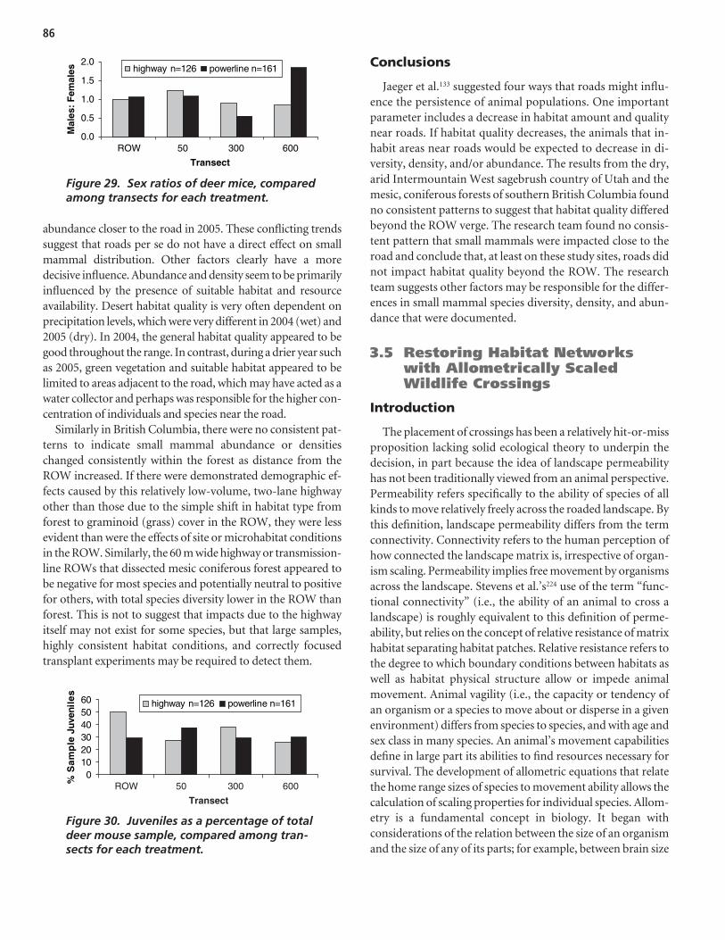
86

abundance closer to the road in 2005. These conflicting trendssuggest that roads per se do not have a direct effect on smallmammal distribution. Other factors clearly have a moredecisive influence. Abundance and density seem to be primarilyinfluenced by the presence of suitable habitat and resourceavailability. Desert habitat quality is very often dependent onprecipitation levels, which were very different in 2004 (wet) and2005 (dry). In 2004, the general habitat quality appeared to begood throughout the range. In contrast, during a drier year suchas 2005, green vegetation and suitable habitat appeared to belimited to areas adjacent to the road, which may have acted as awater collector and perhaps was responsible for the higher con-centration of individuals and species near the road.

Similarly in British Columbia, there were no consistent pat-terns to indicate small mammal abundance or densitieschanged consistently within the forest as distance from theROW increased. If there were demonstrated demographic ef-fects caused by this relatively low-volume, two-lane highwayother than those due to the simple shift in habitat type fromforest to graminoid (grass) cover in the ROW, they were lessevident than were the effects of site or microhabitat conditionsin the ROW. Similarly, the 60 m wide highway or transmission-line ROWs that dissected mesic coniferous forest appeared tobe negative for most species and potentially neutral to positivefor others, with total species diversity lower in the ROW thanforest. This is not to suggest that impacts due to the highwayitself may not exist for some species, but that large samples,highly consistent habitat conditions, and correctly focusedtransplant experiments may be required to detect them.

Conclusions

Jaeger et al.133 suggested four ways that roads might influ-ence the persistence of animal populations. One importantparameter includes a decrease in habitat amount and qualitynear roads. If habitat quality decreases, the animals that in-habit areas near roads would be expected to decrease in di-versity, density, and/or abundance. The results from the dry,arid Intermountain West sagebrush country of Utah and themesic, coniferous forests of southern British Columbia foundno consistent patterns to suggest that habitat quality differedbeyond the ROW verge. The research team found no consis-tent pattern that small mammals were impacted close to theroad and conclude that, at least on these study sites, roads didnot impact habitat quality beyond the ROW. The researchteam suggests other factors may be responsible for the differ-ences in small mammal species diversity, density, and abun-dance that were documented.

3.5 Restoring Habitat Networkswith Allometrically ScaledWildlife Crossings

Introduction

The placement of crossings has been a relatively hit-or-missproposition lacking solid ecological theory to underpin thedecision, in part because the idea of landscape permeabilityhas not been traditionally viewed from an animal perspective.Permeability refers specifically to the ability of species of allkinds to move relatively freely across the roaded landscape. Bythis definition, landscape permeability differs from the termconnectivity. Connectivity refers to the human perception ofhow connected the landscape matrix is, irrespective of organ-ism scaling. Permeability implies free movement by organismsacross the landscape. Stevens et al.’s224 use of the term “func-tional connectivity” (i.e., the ability of an animal to cross alandscape) is roughly equivalent to this definition of perme-ability, but relies on the concept of relative resistance of matrixhabitat separating habitat patches. Relative resistance refers tothe degree to which boundary conditions between habitats aswell as habitat physical structure allow or impede animalmovement. Animal vagility (i.e., the capacity or tendency ofan organism or a species to move about or disperse in a givenenvironment) differs from species to species, and with age andsex class in many species. An animal’s movement capabilitiesdefine in large part its abilities to find resources necessary forsurvival. The development of allometric equations that relatethe home range sizes of species to movement ability allows thecalculation of scaling properties for individual species. Allom-etry is a fundamental concept in biology. It began withconsiderations of the relation between the size of an organismand the size of any of its parts; for example, between brain size

highway n=126 powerline n=161

0.0

0.5

1.0

1.5

2.0

ROW 50 600300

Transect

Mal

es:

Fem

ales

Figure 29. Sex ratios of deer mice, comparedamong transects for each treatment.

0102030405060

% S

amp

le J

uve

nile

s

highway n=126 powerline n=161

ROW 50 600300

Transect

Figure 30. Juveniles as a percentage of totaldeer mouse sample, compared among tran-sects for each treatment.

87

and body size, where animals with bigger bodies have biggerbrains.

Here the relationships between home range size and dif-ferent measures of movement ability (namely, MedianDispersal Distance [MedDD] and linear home range distance[LHRD]) are referred to as allometric because movementability changes in proportion to home range size, which is re-lated to the size of organisms; i.e., there are consistent scalingproperties that can be expressed by equations. Scaling prop-erties can be translated into movement distances characteris-tic of a species. Movements of animals over time can bereferred to as their ecological neighborhood, i.e., a region de-fined by an animal’s movement pattern. Ecological neigh-borhoods for any individual species vary depending uponwhich process is involved. For example, while foraging move-ment distances typically are relatively short, migratory move-ments involve larger ecological neighborhoods. Animals ofsimilar size tend to have similarly sized home ranges and eco-logical neighborhoods. When this is so, it is possible to estab-lish scaling domains that include a few to many species. Forthe purposes of this report, a scale domain refers to a range ofspecies movement distances that are similar, so that severalspecies can be considered to belong to that particular domain.Domains range from small to large, typically with moresedentary animals belonging to a domain characterized byshort movement distances and highly vagile animals belongto a domain characterized by longer movement distances. Tothe extent that species belonging to a specific domain movesimilarly, the placement of wildlife crossings of appropriatetype and configuration at appropriate (allometric) distanceswill promote landscape permeability. Less vagile animalsneed crossings placed closer together, while for more vagileanimals wildlife crossings can be spaced further apart. Theadvantage of domains is that often, a single crossing can beused by many different types of species. There are obvious ad-vantages for both population viability and driver safety whenspecies use crossings and stay off the road surface. Mitigationto decrease the effects of the roaded landscape includes,among other things, the construction of crossings of twogeneral types; those that promote wildlife crossing over theroad, and those that provide passage underneath. The num-ber, type, configuration, and placement of crossings willdetermine whether permeability is restored to the roadedlandscape. The relevant hypothesis is that landscape perme-ability can be improved by the placement of crossings allo-metrically scaled to organism movement characteristics.

Research Approach: Methods and Data

The roaded landscape has both direct (e.g., roadkill) and in-direct (e.g., habitat loss, reduced habitat quality, fragmenta-tion, loss of connectivity and reduced permeability, and barrier

effects) effects on wildlife populations and on ecologicalpatterns and processes.26,30 In particular, animal movement ishindered as road density and traffic volume increase. Spatiallinkage, accomplished by animal movement, is critical becausethe arrays of resources that are essential to population viabilityare usually distributed heterogeneously across the habitat net-work.168 Animal movement can be seasonal migrations120 thattend to be cyclic, dispersal events227 that are usually unidirec-tional,180 or ranging behavior144,228,216 characterized by shorterexploratory movement within a home range or territory. Re-gardless, the ability of animals to move has profound impactson ecological phenomena and processes, including individualfitness, population structure, life history strategies, foraging dy-namics, and species diversity.3,33 Generically, dispersal has beendefined as the movement of organisms, their propagules, ortheir genes away from the source.223,234,59,179,38 Although thisstudy explores the patterns of dispersal distances to understandthe placement of wildlife crossings, clearly the processesinvolved in dispersal underpin our ecological understanding.The phenomena of immigration and emigration, collectivelytermed dispersal, are two of four (births and deaths being theother two) processes that are the least understood in the fieldsof population ecology and life history evolution,75 and repre-sent one of the most significant gaps in how ecologists under-stand animal ecology.22 Wiens246 has argued that dispersal is acomplex process that involves more than just patterns of whereanimals settle. According to Doerr and Doerr75 a more com-prehensive view of dispersal is emerging. Clobert et al.59 haveargued recently that at least three components are involved indispersal: (1) a decision to leave the natal area, (2) a middlephase where new areas are searched and evaluated, and (3) afinal phase that involves choosing a place to settle. This viewsuggests that dispersal distances result from this integrated se-ries of decisions and processes and are influenced by environ-mental and physiological factors, as well as stochastic events.75

Perhaps most critical to our understanding is a dearth of dataregarding these processes. For this report, dispersal is consid-ered to be at the level of individuals and populations. Althoughbarrier effects are not similar across roads, the effects of roadgeometrics (e.g., road type, width, presence of fences) presentsignificant problems to animals, resulting in fragmentedhabitats, disconnected networks, non-permeable or semi-permeable landscapes26 and often isolated populations.43,240,137

A Brief History of Allometric Scaling in Ecology

Allometric scaling in ecology has had a long history. The fol-lowing summary is intended not to cover the historyexhaustively, but only to indicate the line of logic that led tothese analyses. As early as 1909, Seaton209 recognized that animalsize corresponded roughly with home range size. Mohr174 dis-cussed the same relationship specifically for mammalian species.

88

Kleiber141 looked at the scaling relationships between basalmetabolic rate (BMR) and body mass and found that BMR =aM0.75, where M is body mass, a is the allometric coefficient (y intercept), and 0.75 is the allometric scaling exponent. Thegeneral form of the allometric (power law) scaling equation is:

Y = aXb

where Y is the response variable, X is the explanatory variable,a is a scaling constant or coefficient (y intercept), and b is thescaling exponent equal to the regression slope.141,147 McNab165

showed that among mammals, an almost identical power law(scaling exponent) existed between home range size and bodyweight, although Harestad and Bunnell112 found scaling expo-nent values near 1.0 or greater when they looked at differenttrophic levels. They concluded that differences in weight aloneaccounted for a large proportion of the differences betweenmale and female or subadult and adult home range sizes. Theysuggested that inter-trophic (namely, herbivores vs. carnivoresvs. omnivores) scaling functions differed significantly fromeach other. Damuth68 and Brown37 have suggested that the dif-ference between the scaling exponents of 0.75 for energy re-quirements and approximately 1.0 for home range size may beexplained by per capita resource requirements and greater over-lap in home ranges for larger mammals. However, more recentwork by Kelt and Van Vuren,139 working from a large data baseof over 700 publications, found that the scaling relations ofinter-trophic home ranges did not differ and scaled with a slopeof 1.13, greater than either the results of McNab165 or Harestadand Bunnell112. Kelt and Van Vuren139 (p. 637) admit howeverthat the relationship between home range size and body mass“has been perhaps the most difficult to understand.” Recently,Wolff248 and Sutherland et al.227 demonstrated that body size ofmammals is linearly related to dispersal distance when bothvariables were expressed on a log10 scale. However, as Bowmanet al.33 point out, both of these relationships are limited because:(1) some species disperse much further than expected frombody size, and (2) some mammals have larger or smaller homeranges than predicted for a given body size. Given these results,one expects that home range size and dispersal distance shouldco-vary across mammalian species and this is the argument thatBowman et al.33 expand upon. They argue that the residual vari-ance in the body size versus home range, and the body size ver-sus dispersal distance relationships represent real differences invagility independent of body size and therefore the relationshipbetween dispersal distance and home range size should co-varyacross mammal species after the effects of body size are removed.

The Dispersal Distance Connection

Dispersal is a fundamental element of demography,7 col-onization,117 and gene flow182 but dispersal movements are

perhaps the least well understood of ecological phenom-ena.227 Bowman et al.33 showed that dispersal distance is ac-tually more closely related to home range size (R2 = 0.74)than to body size (R2 = 0.60), where R2 is the proportion ofthe variance explained by home range size and body size, re-spectively. This discovery is significant because dispersal dis-tances, as well as ranging and migratory behavior, representanimal movement across the landscape. Bowman et al.33

found that when body size effects were removed, the slope ofthe relationship of the residuals of dispersal distance re-gressed against the residuals of home range size was not sig-nificantly different from 0.50 (F = 31.6, df = 1, 32, P = 3.2 x10−6, S.E.E. = 0.54), a result with very important ramifica-tions. The significance is this: Dispersal distance is a linearmeasure, while home range area is a squared linear measure.Because X0.05 is equal to the square root of X, and because Xin the scaling equation is equal to home range area, takingthe square root of the home range area yields a linear di-mension of home range, allowing dispersal distance to be re-lated to home range size by a single constant value.

Bowman et al.33 found that maximum dispersal distance(MaxDD) was related to home range size (HR) by the equation:

MaxDD = 40 (linear dimension of HR)

and median dispersal distance (MedDD) was related to homerange size by the equation:

MedDD = 7 (linear dimension of HR)

Because home range size is easy to measure and is readilyavailable in published literature, appropriate scaling functionsfor deciding the general ecological neighborhood of specieswould appear to be easy to obtain. If so, they provide the nextstep to inform the placement of wildlife crossings.

What is an Ecological Neighborhood?

The concept of ecological neighborhoods is defined bythree properties: (1) an ecological process (e.g., inter-patchmovement), (2) a time scale relevant to the process, and (3)an organism’s activity during that time period.3 Additionally,no single temporal or spatial scale is appropriate to representthe mix of processes that influence individual and species re-sponses through time and space; hence, several ecologicalneighborhoods exist, depending upon what process isinvolved (e.g., foraging, territory defense, migration). Char-acteristically, for mobile organisms, the ecological neighbor-hood for a given process is the region within which thatorganism is active, definable by its movement patterns. In-deed, Addicott et al.3 (p. 343) suggest that “for neighbor-hoods. . . . the most appropriate indicator of activity may bea measure of net movement of individuals . . . . One [such in-dicator] is the direct measurement of dispersal distances.”

89

Source: Redrawn from Addicott et al.3

0

B

A

50

95

0

50

95

N1 N2

Na Nb

inter-patchmovement

spatial unit (distance)

foraging

% c

um

ula

tive

dis

trib

uti

on

of

mo

vem

ent

Figure 31. Theoretical relation-ship between the cumulativedistribution of organism move-ment and spatial scale, i.e., eco-logical neighborhood.

Figure 31 shows the theoretical relationship betweenmovement and two ecological neighborhoods where N1 andN2 represent two different spatial units related to two distinctanimal activities. The horizontal and vertical dashed lines in-dicate different “neighborhood sizes” for the two different ac-tivities (dotted lines, Figure 31A). In general, thinking aboutlandscape permeability involves larger spatial units. In thisexample, foraging involves a smaller ecological neighborhood(N1), but inter-patch movements, which might include find-ing mates or additional resources, typically involves largerspatial areas (N2), i.e., larger ecological neighborhoods, andmay be equated with some measure of dispersal.

When roads cross the landscape, the larger ecologicalneighborhoods that animals use (e.g., related to inter-patchmovement) may be intersected. When such intersection oc-curs, barrier effects become apparent. In Figure 31, both inter-patch interactions involving movement over large distancesand the movements related to the shorter foraging activitiesare defined by a cumulative distribution of distances moved.Each line in Figure 31B represents a cumulative distributionof movements with an associated neighborhood size (N1, N2)for foraging and inter-patch movements. The decision crite-rion is 95% of all movements related to either process,3 but isarbitrary; it could easily be different. Given the results fromBowman et al.,33 the problem of deciding an appropriate spac-ing for wildlife crossings is now somewhat easier because plan-ners can relate ecological neighborhoods of activity requiredby animals to survive to a distance measure. Usually, ecologi-cal neighborhoods are defined for each individual species.However, it is unreasonable from a management perspective

to attempt to place crossings allometrically for each individ-ual species. Some grouping of species is desirable, especially iftheir home range sizes are similar in size and have small amongversus between group differences.

Domains of Scale

To the extent that (1) similarities in home range sizes existfor groups or guilds of species and (2) there are recognizabledifferences between groups, it should be possible to deter-mine a few effective scale domains that characterize themovements of each group. Theoretically, boundaries of scaledomains should be recognized where the differences (e.g., indispersal distances) increase as transitions between domainsare approached. If possible, then the recognition of a fewgroups or guilds composed of similarly sized species withsimilar home range domains is an important first step indetermining the spatial location for effective crossings formost species. The assumption is that similarly sized animalswill use similar types and similarly spaced crossings.However, there may be inter-trophic differences (i.e., carni-vores, herbivores, and omnivores may scale differently). If so,consideration should be given when deciding on the type andplacement of wildlife crossing. The calculation of guild-specific movement domains is an important step in allomet-rically placing wildlife crossings. To the extent that thesearguments hold, the placement of appropriate types of cross-ings can be accomplished in a scale-informed and sensitivemanner, resulting in a more permeable roaded landscape thateffectively restores the broader habitat network.

Wildlife Crossings and Inter-Patch Movements

The intent, of course, of establishing allometrically scaledwildlife road crossings is to enhance inter-patch movements.Most if not all organisms live in discontinuous habitat patchesof suitable habitat within a matrix of less suitable habitat thatis embedded in larger, naturally heterogeneous landscapes,34

and the presence of roads generally increases patch isolation.Ecologically, animal vagility and movement ability determineif populations are isolated in a naturally heterogeneous land-scape.3,34 Although important, inter-patch movement has notbeen extensively studied and few empirical estimates of move-ment rates or effects on populations have been derived.34 It isunclear what amount of inter-patch movement is needed toinfluence the dynamics of populations divided by roads.While real problems exist in gathering inter-patch movementdata,34 Bowne and Bowers34 conducted a database search todetermine the extent that documented rates were available.

From a review of 415 published articles, they found that for89 species-system combinations, roughly 15% of all individ-uals in a population moved between habitat patches each

90

generation. More importantly, population rates (i.e., birthrates, death rates, recruitment, survival) were either positive(n = 28) or neutral (n = 14) over 95% of the time, but nega-tive in only two instances (<5%). This finding underscoresthe necessity of restoring functional connectivity to theroaded landscape. Inter-patch movements may involverelative short distances or long-distance dispersal. Shortermovements are more frequent, while longer dispersaldistances are typically rare.232

Description of Methods

Bowman et al.33 developed their home range dispersal re-lationships for mammals from data given in Harestad andBunnel.112 For this study, the Harestad and Bunnell112 datawas augmented with the species home range list given inHolling122 Appendix 7 to amass a total of 103 mammalianspecies from around the world (Appendix G). Other sourcesof home range information are available, but the Harestadand Bunnell112 data are well known, are accepted by ecolo-gists, and have been used to advance the allometric scaling ofmammals.139 The Holling122 paper increased the number ofspecies for which reliable home range data are available. Onlydata for species with at least five replicates were used in theHolling paper. Some species do not occur in North America,but were included because (1) their home range area infor-mation was reliable and (2) they provided a reasonablesample size from which to develop reliable dispersal distancedomains. Elimination of duplicate entries left 103 species.A caveat is necessary here. Home range size varies over timefor individuals and for populations. The values used in thisstudy are the best representative values available for thespecies. Individual home ranges will no doubt vary aroundthese mean values.

The Bowman et al.33 equations were then used to calculateMedDD (i.e., 7* √HR) and LHRD (i.e., √HR) from these homerange data and from data in 10 papers that listed daily move-ment distances (DMD) to explore if a consistent relationshipexisted between DMD and the MedDD. If a consistent rela-tionship exists, then three different scaling domains could bedeveloped to inform the placement of crossings. All threetransformations (MedDD, LHRD, and DMD) representdifferent ecological neighborhoods for individual species.

After the distance conversions were calculated, the researchteam applied a hierarchical monothetic agglomerative cluster-ing technique using Ward’s linkage method with a Euclideandistance measure as the sorting strategy162 to detect naturalbreaks in the data. Monothetic refers to the clustering of onevariable (i.e., the measure of home range); agglomerative refersto the procedure of clustering groups of species and meanssuch that each group starts as a single species and is clustered(agglomerated) by some linkage method. Euclidean distance

was used because it is one of the simplest measures and isroughly equivalent to the linear distance between any twomeasures. The shorter the distance, the more similar the meas-ures and the more likely the species involved will be includedin a group. Ward’s method is based on minimizing the sum ofthe squares of distances from each individual species to thecentroid of its group.161 The method produces a clusteringmatrix and a dendrogram of the species groups. The researchteam chose to represent the data to the sixth cluster (i.e., to the0.16-mi level).

After the natural breaks were detected, frequency distribu-tions for the species home range areas that had been convertedto the median dispersal distances and to the linear home rangedistances were calculated. The frequency distributions areequivalent to scale domains that represent similar scaling bygroups of species. The research team also compared trophiclevel (i.e., carnivore, herbivore, and omnivore) median disper-sal distances to determine if differences existed. The researchteam looked at a sample of 10 papers that provided daily move-ment data and examined if a consistent relationship existedbetween daily movement distances and median dispersal dis-tance. Because median dispersal distance and linear homerange distances are derived from home range area, if there wasa relationship, it should apply to any of these measures.

Finally, the research team compared the options for spac-ing wildlife crossings and presented the most feasible scalingdomains for large mammals that are most likely to be in-volved in serious animal–vehicle collisions.

Findings and Results

Mammalian Species Scaling: Median Dispersal Distance

When the median dispersal distance equation (7 * √ HomeRange) was used, mammalian species dispersal distancesranged from 0.06 mi for the northern pocket gopher (Tho-momys talpoides) to 168.46 mi for the wolverine (Gulo gulo).Of 103 species, 50% scaled to less than 4 mi (Figure 32, Table34). More than 70% of species had median dispersal distancesof 8 mi or less. When median dispersal distances weregrouped by a hierarchical polythetic agglomerative clusteringtechnique,162 55.4% scaled longer than 3.05 mi (Figure 33).

Not all trophic levels (i.e., carnivores, herbivores, and om-nivores) scale similarly. One expects that carnivores, whoseprey is the herbivore component of the community, wouldtravel greater distances and have larger home ranges. Simi-larly, herbivores, whose primary food resource includesplants, would be expected to scale differently and indeed thatis the case. Indeed, MedDD for omnivores ranged from 0.39to 50.05 mi, herbivores ranged from 0.06 to 16.47 mi, andcarnivores from 0.14 to 168.46 mi (Figures 34 and 35). It is

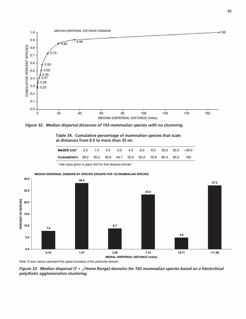
91

MedDD (mi)* 0.5 1.0 2.0 3.0 4.0 6.0 8.0 20.0 35.0 >35.0

Cumulative% 28.2 35.0 40.8 44.7 50.5 63.2 70.9 85.4 90.3 100

*mile value given is upper limit for that distance domain

Table 34. Cumulative percentage of mammalian species that scale at distances from 0.5 to more than 35 mi.

00.0

0.1

0.2

0.3

0.4

0.5

0.6

0.7

0.8

0.9

1.0

20 40 60 80

MEDIAN DISPERSAL DISTANCE (miles)

CU

MU

LAT

IVE

PE

RC

EN

T S

PE

CIE

S

100

1.00

0.900.85

0.45

0.35

0.23

0.41

0.73

0.53

0.50

120 140 160

MEDIAN DISPERSAL DISTANCE DOMAINS

Figure 32. Median dispersal distances of 103 mammalian species with no clustering.

MEDIAN DISPERSAL DOMAINS BY SPECIES GROUPS FOR 103 MAMMALIAN SPECIES

7.8

28.2

8.7

23.3

4.9

27.2

0.0

5.0

10.0

15.0

20.0

25.0

30.0

0.16 1.07 3.05 7.15 10.71 >11.00

MEDIAL DISPERSAL DISTANCE (miles)

PE

RC

EN

T O

F S

PE

CIE

S

Note: X-axis values represent the upper boundary of the particular domain.

Figure 33. Median dispersal (7 * Home Range) domains for 103 mammalian species based on a hierarchicalpolythetic agglomerative clustering.

92

COMPARISON OF TROPHIC MEDIAN DISPERSAL DISTANCES

4.97.3

12.2

24.4

7.3

43.9

14.6

53.7

4.9

12.2

2.4

12.2

0.0

19.0

9.5

42.9

4.8

23.8

7.8

28.2

8.7

23.3

4.9

27.2

CARNIVORES HERBIVORES OMNIVORES TOTAL SPECIES

0.00

10.00

20.00

30.00

40.00

50.00

60.00

0.16 1.07 3.05 7.15 10.71 >11

DISTANCE (miles)

PE

RC

EN

T O

F S

PE

CIE

S

Figure 35. Comparison of the median dispersal distance domains of carnivores, herbivores, and omnivores.

Figure 34. Carnivores, herbivores, and omnivores show different mediandispersal distances.

clear that wildlife crossings placed 6 mi or more apart will notprovide either permeability or adequate crossing opportuni-ties for approximately 63% of the mammalian species likelyto be found on the landscape. Clearly median dispersaldistances provide only the extreme limit and by themselvescannot fully inform the placement of wildlife crossings.

Mammalian Species Scaling: Linear Dimension Distance

At the other end of the spectrum, the linear dimension ofthe home range (√HR) provides a scaling that more closely ap-proximates the majority of movements made by mammalianspecies, which typically move within their home range formost of the year. During spring and fall of course, juvenile an-imalsusually make longer migratory movements.227 When lin-ear movement domains were used to place multiple wildlife

crossings according to a mile-marker spacing, approximately12% of species would be likely to cross at a distance of 7 mi,approximately 30% at 3.0 mi, and approximately 64% atcrossing distances of 1 mi. All species would likely cross at aspacing distance of 0.16 mi (Figure 36). Consequently, maxi-mum landscape permeability is more likely when placingwildlife crossings based on the linear scale domains.

Mammalian Species Scaling: Daily Movement Distance

It is possible that daily dispersal distances may provide analternative scenario for placing wildlife crossings; however,daily movement distances are difficult to collect and often notuniformly collected. For example, Krausman et al. (unpub-lished data) collected movement data on 46 mule deer(Odocoileus hemionus) whose movements were followed

93

HIERARCHICAL MONOTHETIC AGGLOMERATIVE CLUSTERING

35.9233.98

17.48

6.80

3.881.94

0

5

10

15

20

25

30

35

40

0.16 1.07 3.05 7.15 10.71 >11LINEAR DISTANCE DOMAINS (mi)

PE

RC

EN

T S

PE

CIE

S

Figure 36. Linear ( Home Range) dispersal domains for 103 mammalian species using hierarchicalmonothetic agglomerative clustering.

using radio telemetry from 1999 to 2003 (Figure 37). Record-ing of the relocations occurred at about 24-hour intervals.The data indicate that the majority of individual daily move-ments were short with 85.1% being 1,000 meters or less.

Certainly deer moved greater distances; however, recordingonly two locations, one at the beginning of the period and oneat the end, essentially straightens what is a much more tortu-ous movement pathway. This movement oversimplification isthe major problem of using daily movement data. The mostaccurate method for assessing daily movement distanceswould measure the trajectory of the animal’s pathway at shortintervals for several 24-hour periods using GPS collars set torecord locations frequently, and then take a mean value. Sea-sonality affects daily movement patterns, so an adequate sam-ple is needed. Typical methods for collecting daily movementdistance data include following the trajectory for a few hoursand then extrapolating daily movement distance, or takingonly a few (often as few as two) telemetry relocations over a24-hour period and then measuring the straight-line distancebetween relocations. This method seriously underestimatesdaily movement distances.

However, if there is a consistent relationship between dailymovement distances and median dispersal distance, with prop-erly collected data (e.g., by using continuously monitoring GPSradio transmitting collars), a conversion factor can be developedfor daily movement distance domains that might help informwildlife crossing distance. The research team initially found 10species for which daily movement data were available (Table 35).Each individual movement represents the straight-line distancebetween two relocations taken approximately 24 hours apart.

The relationship between median dispersal distance and dailymovement distance for all 10 species is quite loose, with a meanof 61.95, S.D. = 83.62, P = 0.05. Mean values for carnivoresalone = 42.66, S.D. = 84.45, P = 0.05, and for herbivores, mean =96.4, S.D. = 93.27, P = 0.05. The variation of the ratios betweenthe median dispersal and daily movement distances is too largeto give a realistic and reasonable conversion factor. With a largersample, the results might be different. Alternatively, when accu-rate multiple daily movement distance estimates become avail-able for those large species that account for the greatest safety riskwhen WVCs occur, then a proper daily movement distance scal-ing can be developed for individual species. Additional work willbe necessary to see if those data exist.

Interpretation, Appraisal, and Applications

There are at least three potential options in spacing wildlifecrossings using allometric distance domains. All involve scalingto home range area and are (1) the median dispersal distance

, (2) a linear dimension of home range ( HR), and(3) a scaling measure related to daily dispersal distance. Usingthe linear dimension of the species home range to develop scaledomains is most conservative and places crossings closesttogether. The implication is that crossings are no further apartthan the linear dimension of the largest home range in the scaledomain.

Using the square root of the home range to establish scal-ing domains to inform the placement of wildlife crossings ismost reasonable because shorter dispersal distances by juve-niles are more frequent.227 Additionally, animal fidelity to

7 * HR( )

94

Species TLa MedDDb (m) DMDc (m) Ratio Swift fox (Vulpes velox)d C 19,712 18,500 1.07 European marten (Martes martes)e C 8,573 5,100 1.68 Eurasian lynx (Lynx lynx)f C 30,128 3,800 7.93 Polecat (Mustela putorius)g C 9,899 1,097 9.02 Wolverine (Gulo gulo)h C 271,109 1,400 193.60 Lemming (Dicrostonyx groenlandicus)i H 213 15 14.08 Mule deer (Odocoileus hemionus)j H 11,823 311 38.02 Moose (Alces alces)k H 24,400 220 111.90 Cotton rat (Sigmodon hispidus)l H 4,670 21 221.60 Wild boar (Sus scrofa)m O 274,485 13,280 20.67 atrophic level: C = carnivore, H = herbivore, O = omnivore; bmedian dispersal distance; cdaily movement distance; dCovell et al.64; eZalewski et al.250; fMoa et al.173; gBrzezinski et al.39; hRenzhu et al.198;iSchmidt et al.207; jKrausman, unpublished data; kCourtois et al.63; lSulok et al.226; mSpitz and Janeau218.

Table 35. Daily movement distances for 10 mammalian species.

Figure 37. Distribution of daily movement distances of 46 telemetered mule deer from 1999 to 2003.

home range areas suggests that shorter individual movementdistances predominate among all sexes and ages. Thus, thelinear scale approach would appear to promote greatestpermeability (Figure 38, Table 36). A less conservativeapproach uses the median dispersal distance,33 i.e., seventimes the linear dimension of home range, as the criteria fordeveloping the scale domains. Longer distance dispersal doesoccur less frequently but is important for recolonizing areasas well as gene flow.227 An intermediate approach might usedaily movement distances to develop distance domains. Typ-ically, one might expect that mammals would travel signifi-cantly longer distances in their search for resources. To theextent that daily movement data are available for species, al-

lometric domains can be developed to inform the placementof wildlife crossings. The sample given in Table 35, however,suggests that a large sample will be needed to extract the rela-tionship, if it exists.

Conclusions

Placing Crossings for Large Mammals

The involvement of large terrestrial mammals inwildlife–vehicle collisions tends to result in greater vehicledamage and greater potential for human injury and deaththan the involvement of smaller body-sized animals. Large-

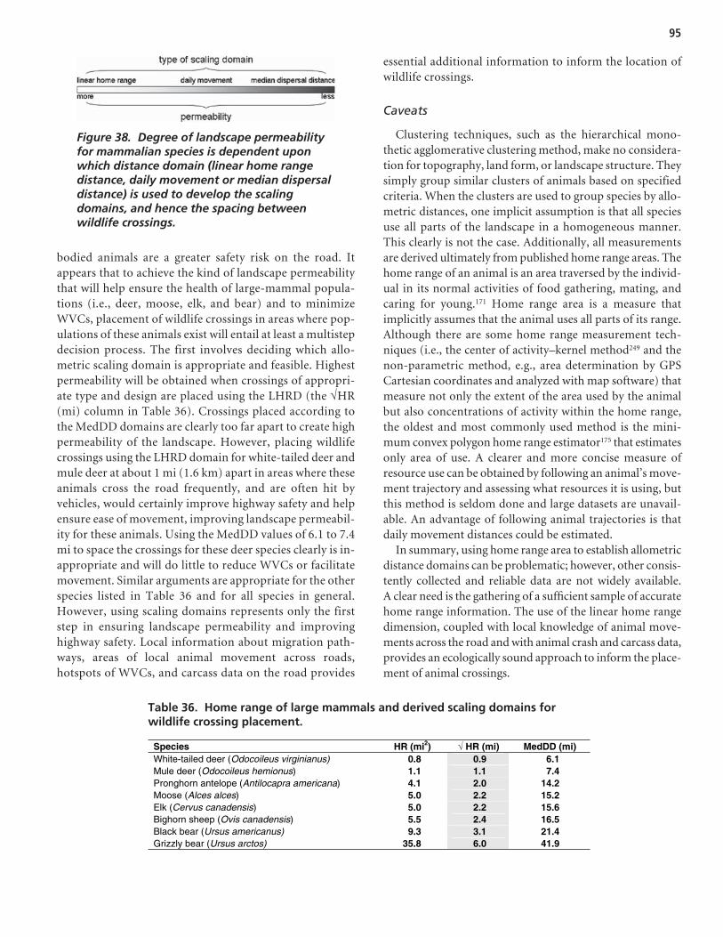
95

Figure 38. Degree of landscape permeabilityfor mammalian species is dependent uponwhich distance domain (linear home rangedistance, daily movement or median dispersaldistance) is used to develop the scaling domains, and hence the spacing betweenwildlife crossings.

Species HR (mi2) HR (mi) MedDD (mi) White-tailed deer (Odocoileus virginianus) 0.8 0.9 6.1Mule deer (Odocoileus hemionus) 1.1 1.1 7.4Pronghorn antelope (Antilocapra americana) 4.1 2.0 14.2Moose (Alces alces) 5.0 2.2 15.2Elk (Cervus canadensis) 5.0 2.2 15.6Bighorn sheep (Ovis canadensis) 5.5 2.4 16.5Black bear (Ursus americanus) 9.3 3.1 21.4Grizzly bear (Ursus arctos) 35.8 6.0 41.9

Table 36. Home range of large mammals and derived scaling domains forwildlife crossing placement.

bodied animals are a greater safety risk on the road. Itappears that to achieve the kind of landscape permeabilitythat will help ensure the health of large-mammal popula-tions (i.e., deer, moose, elk, and bear) and to minimizeWVCs, placement of wildlife crossings in areas where pop-ulations of these animals exist will entail at least a multistepdecision process. The first involves deciding which allo-metric scaling domain is appropriate and feasible. Highestpermeability will be obtained when crossings of appropri-ate type and design are placed using the LHRD (the √HR(mi) column in Table 36). Crossings placed according tothe MedDD domains are clearly too far apart to create highpermeability of the landscape. However, placing wildlifecrossings using the LHRD domain for white-tailed deer andmule deer at about 1 mi (1.6 km) apart in areas where theseanimals cross the road frequently, and are often hit byvehicles, would certainly improve highway safety and helpensure ease of movement, improving landscape permeabil-ity for these animals. Using the MedDD values of 6.1 to 7.4mi to space the crossings for these deer species clearly is in-appropriate and will do little to reduce WVCs or facilitatemovement. Similar arguments are appropriate for the otherspecies listed in Table 36 and for all species in general.However, using scaling domains represents only the firststep in ensuring landscape permeability and improvinghighway safety. Local information about migration path-ways, areas of local animal movement across roads,hotspots of WVCs, and carcass data on the road provides

essential additional information to inform the location ofwildlife crossings.

Caveats

Clustering techniques, such as the hierarchical mono-thetic agglomerative clustering method, make no considera-tion for topography, land form, or landscape structure. Theysimply group similar clusters of animals based on specifiedcriteria. When the clusters are used to group species by allo-metric distances, one implicit assumption is that all speciesuse all parts of the landscape in a homogeneous manner.This clearly is not the case. Additionally, all measurementsare derived ultimately from published home range areas. Thehome range of an animal is an area traversed by the individ-ual in its normal activities of food gathering, mating, andcaring for young.171 Home range area is a measure thatimplicitly assumes that the animal uses all parts of its range.Although there are some home range measurement tech-niques (i.e., the center of activity–kernel method249 and thenon-parametric method, e.g., area determination by GPSCartesian coordinates and analyzed with map software) thatmeasure not only the extent of the area used by the animalbut also concentrations of activity within the home range,the oldest and most commonly used method is the mini-mum convex polygon home range estimator175 that estimatesonly area of use. A clearer and more concise measure ofresource use can be obtained by following an animal’s move-ment trajectory and assessing what resources it is using, butthis method is seldom done and large datasets are unavail-able. An advantage of following animal trajectories is thatdaily movement distances could be estimated.

In summary, using home range area to establish allometricdistance domains can be problematic; however, other consis-tently collected and reliable data are not widely available.A clear need is the gathering of a sufficient sample of accuratehome range information. The use of the linear home rangedimension, coupled with local knowledge of animal move-ments across the road and with animal crash and carcass data,provides an ecologically sound approach to inform the place-ment of animal crossings.

96

3.6 Interpretation of Research Results

The sections on the Phase 2 research studies (safety [3.1], ac-curacy modeling [3.2], hotspot analysis [3.3], small mammalsand putative habitat degradation effects [3.4], allometric plac-ing of wildlife crossings [3.5]) contain important informationand suggestions for implementation. In particular, Sections 3.1,3.2, and 3.3 address different ways to achieve similar purposesand therefore potentially may be confusing for the reader. Forexample, Section 3.1 involves analyses of WVCs and road envi-ronment data from state DOT sources. Section 3.2 involves aninvestigation into the relative importance of factors associatedwith wildlife killed on the road using two different datasets: onebased on high-resolution, spatially accurate location data (<3 merror) representing an ideal situation and a second datasetcreated from the first that was characterized by lower resolutiondata (<_ 0.5 mi or 800 m, i.e., mile-marker data) and likely typi-cal of most transportation agency data. Section 3.3 investigatesseveral wildlife kill hotspot identification clustering techniqueswithin a GIS framework that can be used in a variety of land-scapes. This section on the interpretation of the research resultswill guide the reader in understanding these sections.

The safety research (Section 3.1) is most effectively usedwhen the purpose is to assess if a specific mitigation has beensuccessful in reducing WVCs to improve public safety. Itemploys the use of SPFs, predictive models for AVCs. SPFstypically relate the response variables (AVC data and/orroadside carcass collection data) to the explanatory variables(physical roadway and roadside characteristics; oftenreferred to as road geometrics). Other explanatory variablesthat animals respond to (e.g., topography, vegetative cover,and other off-road variables) are not among these variablesthat are readily available within the typical DOT safety data-bases. Hence, this approach will result in some unexplainedvariation, because the safety approach limits the explanatoryvariables to road geometrics. Regardless, this approach isvaluable because only these lower levels of data availabilitymay exist in some jurisdictions.

The SPF approach is statistically correct and accounts for“regression to the mean” problems. It makes use of three dif-ferent levels of road data commonly available. The first level re-quires data on (1) road length and (2) ADDT. The second leveladds the requirement that road segments be classified as flat,rolling, or mountainous terrain. The third level incorporatesthe data used in levels 1 and 2, but includes additional roadwayvariables such as average lane width. The safety approach hasseveral applications and can be used to:

• Identify collision-prone locations for existing or proposedroads for all collision types combined or for specific targetcollision types

• Aid in the evaluation, selection, and prioritization of po-tential mitigation measures; and

• Evaluate the effectiveness of mitigation measures alreadyimplemented.

An important caveat is that the safety approach does notaddress any aspect of wildlife population response. As themodels stand, their primary application is for the safety man-agement of existing roads as opposed to design or planningapplications for new or newly built roads. Significantly, thebefore-after analysis may be judged as successful from a roadsafety perspective, while at the same time the wildlife popu-lation concerned may be significantly reduced.

A second aspect of the safety effort was to investigate thehypothesis that roadside carcass removal data not only indi-cate a different magnitude for the WVC problem, but mayalso show different spatial patterns than reported WVC data,and lead to the identification of different roadway locationsfor potential WVC countermeasures. The magnitude andpatterns of location-based WVC reports and deer carcass re-moval datasets from Iowa were compared qualitativelythrough visual GIS plots and quantitatively (e.g., frequencyper mile). Police-reported WVC information, deer carcassremovals, and deer salvage data were evaluated. Resultsshowed that the number of deer carcasses removed from theroad was approximately 1.09 times greater than the numberof WVCs reported to the police. The number of salvaged andunsalvaged deer carcasses, on the other hand, was approxi-mately 1.66 times greater. Clearly, the choice of the databaseimpacts whether a particular roadway segment might beidentified for closer consideration. The message here is thatthe choice of the database used to define and evaluate theWVC problem and its potential countermeasures requirescareful consideration. Recommendations are provided in thisreport about how the databases might be used appropriatelyand how the data can be most profitably collected.

To understand the important variables that account forWVCs, then environmental variables must be considered thatare not normally included in datasets available from DOTs.The safety research recognized that variables other than road-related variables might be important. In the accuracy model-ing (Section 3.2), the research team used 14 ecological fieldvariables, 3 distance-to-landscape-feature variables, and 5 GIS-generated buffer variables as explanatory variables to assesstheir relative importance in explaining where ungulates werekilled on the road. Further, the research team assessed whetherthe spatial accuracy of these datasets was important in identi-fying the significant explanatory variables. Spatially accuratedata were discovered to make a difference in the ability ofmodels to provide not just statistically significant results butmore importantly, biologically meaningful results for trans-portation and resource managers responsible for reducing

97

WVCs and improving motorist safety. Hence, these modelsare especially applicable when it is important to locate hotspotareas of WVCs and hence wildlife crossings during the designand planning of new roads.

The hotspot analysis (Section 3.3) investigated WVChotspot identification techniques, taking into account differ-ent scales of application and transportation managementconcerns. Studies of WVCs have demonstrated that they arenot random occurrences but are spatially clustered. Data onhotspots of WVCs can aid transportation managers in in-creasing motorist safety and habitat connectivity for wildlife.Knowledge of the geographic location and severity of WVCsis a prerequisite for devising mitigation schemes that can beincorporated into future infrastructure projects (e.g., bridgereconstruction, highway expansion). Many of the studiescharacterizing WVCs have appeared in scientific andmanagement-focused journals and often include differentconclusions or recommendations for managers to consider indesigning wildlife-friendly highways. However, lacking arebest management practices for identifying WVC hotspotsbased on current knowledge and technology to help guideplanning and decision making. Few studies specificallyaddress the nature of WVC hotspots or their use and appli-cation in transportation planning. Because WVCs representa distribution of points, recently developed and refined clus-tering techniques can be used to identify hotspots.

As an initial step, the researchers used the linear nearestneighbor index (a simple plotting technique) to assesswhether the location of dead ungulates found on roads as aresult of WVCs was random. The results, however, are onlyan indicator of first order spatial randomness, i.e., an indi-cator to what extent the animal kill locations may beclumped. Simple plotting most often results in collisionpoints being tightly packed together, in some cases directlyoverlapping with neighboring WVC carcass locations, thusmaking it difficult to identify distinct clusters, i.e., where thereal high-risk collision areas occurred. Modeling or analyt-ical techniques permit a more detailed assessment of whereWVCs occur, their intensity, and the means to beginprioritizing highway segments for potential mitigationapplications. Hence, more definitive analytical clusteringtechniques are needed.

The research team used Ripley’s K statistic of roadkills, near-est neighbor measurements (using CrimeStat software), anddensity measures to more formally identify WVC hotspotlocations, once roadkill locations were found to be unevenlydispersed. The Ripley’s K analysis clearly shows the spatialdistribution of WVCs and the importance of broad-scalelandscape variables (such as elevation and valley bottomsin a mountain environment). Further, the locations of high-intensity roadkill clustering within each area can help to focusor prioritize the placement of mitigation activities, such aswildlife crossings or other countermeasures, on each highwaysegment. The research team found that the nearest neighbor(CrimeStat) approach was useful for identifying key hotspotareas on highways with many roadkills because it, in essence,filters through the roadkill data to extract where the most prob-lematic areas lay. The density analysis approach identifiedmore hotspot clusters on longer sections of highway. Althoughthe density analysis approach appears to be less useful to man-agement, it may be a preferred option where managers areinterested in taking a broader, more comprehensive view ofwildlife–vehicle conflicts within a given area. Such a broaderview may be necessary not only to prioritize areas of conflictsbut also to plan a suite of mitigation measures. The location ofthe larger clusters produced by the density analysis could betracked each year to determine how stable they are or whetherthere is a notable amount of shifting between years or overlonger time periods. This type of information will be of valueto managers in addressing the type of mitigation and intendedduration (e.g., short-term vs. long-term applications).

The identification and delineation of WVC clusters, whichoften vary widely in length depending on distribution andintensity of collisions, facilitates between-year or multiyearanalyses of the stability or dynamics of WVC hotspot loca-tions. The WVC data that transportation departmentscurrently possess are suitable for meeting the primary objec-tive of identifying hotspot locations at a range of geographicscales, from project-level (<50 km of highway) to largerdistrict-level or state-wide assessments on larger highwaynetwork systems. The spatial accuracy of WVCs is not of crit-ical importance for the relatively coarse-scale analysis of wherehotspots are located. Any of the analytical clustering tech-niques can be used when more detailed information is needed.

98

The final product of this research is an interactive decisionguide that provides clearly written guidelines for the selec-tion, configuration, and location of crossing types, as well assuggestions for the monitoring and evaluation of crossing ef-fectiveness, and their maintenance. The interactive decisionguide can be found at the URL http://wildlifeandroads.org.The basic outline of the interactive decision guide is hierar-chical. The user can use the Navigation Box to enter the siteat any step. The hyperlink for each step is located within thebox of each step. The outline of the Guide is shown in Fig-ure 39. Clicking on “What should I know?” under Site Naviga-tion takes users to a page where they can learn about the wildlifeissues they need to consider in a road project (Figure 40).

If the user is familiar with these issues, the logical startingplace is the Decision Guide. When “The Decision Guide” linkis clicked under Site Navigation, the Decision GuideOverview (Figure 39) appears. When the Step 1 “ResourceEvaluation” box is clicked, Figure 41 appears.

When the cursor passes over each of the boxes or triangles(1.1, 1.2, and 1.3), the user will see a description of Step 1 withits three substeps: 1.1 Identify Scope of TransportationPlan/Project, 1.2 Identify Wildlife and Fisheries Issues, and 1.3If a Mitigation Need: Identify Goals and Objectives. Also in-cluded on the page are links to other helpful websites. Similarly,Figure 42 appears when the box for step 1.1 is clicked.

The user can scroll down though the step to view the restof the information. The other steps are accessed in a similarway. For example, when the box for step 1.2 is clicked, theuser will see the page as shown in Figure 43.

Again, the user can scroll down to see the rest of theinformation.

Step 2, Identify Solutions, is the centerpiece of the inter-active decision guide. Step 2 is where detailed guidance isprovided to users for the selection, configuration, and loca-tion of wildlife crossings and their monitoring for effective-ness and maintenance. Six second-level steps are providedwhere users can learn about the types of mitigation for pass-

ing wildlife safely over, under, and across transportationcorridors (Step 2.1); how to place that mitigation (Step 2.2);how to determine configuration (Step 2.3); how to deter-mine maintenance needs (Step 2.4); how to begin a cost-effectiveness analysis (Step 2.5); and how to determinemonitoring and the evaluation plan (Step 2.6). Each of thesix second-level steps can be clicked for third-level informa-tion germane to that step. Step 2 is accessible by clicking theStep 2 “Identify Solutions” box and the page shown inFigure 44 appears.

Any of the steps can be accessed for additional informa-tion. For example, if Step 2.1 is clicked, these third order stepsappear, each with accessible additional information:

2.1.1 Identify Species to Benefit from Potential Mitigation2.1.2 Identify Ecological Processes (Water Flow, Animal

Movement, Other)2.1.3 Identify Landscape and Topographic Features that

May Affect Movement and Migration 2.1.4 Identify Engineering and Maintenance Concerns2.1.5 Weigh Cost Concerns with Potential Benefits2.1.6 Identify Appropriate General Wildlife Crossing

Type2.1.7 Other Mitigation Options2.1.8 References

Step 3, Select and Create a Plan, is a decision node where allthe information from previous steps are integrated into thelarger planning and decision-making process. If the planninglevel is controlled by the National Environmental Policy Act(NEPA) process, then Step 3 corresponds to the Record ofDecision or Decision Notice. Each agency will have its ownprocedure. The major product of Step 3 is a decision on the mit-igation appropriate for the project. When the user clicks theStep 3 diamond (a decision node), Figure 45 appears.

Each substep of Step 3 is linked and provides detailed in-formation on documenting decisions in the Implementation

C H A P T E R 4

Decision Guide

99

Figure 39. Interactive Decision Guide Overview.

Plan, developing maintenance agreements, and identifying animplementation liaison.

When the user clicks on the Step 4 “Construction” box,Figure 46 appears. Construction is the beginning of the im-plementation phase of the project and after the crossing hasbeen built, a monitoring and evaluation phase, often neglectedwhen road projects are built, begins. Only through monitor-ing and evaluating performance against a priori expectationsof performance, e.g., successful passage of the intendedspecies, can biologists and engineers understand what cross-ings work and what need modifications.

When the user clicks on the Step 5 “Monitor & Evaluate”box, Figure 47 appears. The user can scroll down to read therest of the information contained on the page and can clickon the icons for Steps 5.1, 5.2, and 5.3 for pertinent informa-tion on Adaptive Management.

The following classes of data are linked to the query func-tions (Figure 48). For example, all the pictures on the websitehave linked key words so that a query asking about specificspecies, places, or crossing types will return pictures thatmatch the query. Hence, a picture of a wildlife crossing for un-gulates, which is along a stream and currently under con-struction in Montana, is linked with the query functions byany of the following key words: ungulate, deer, elk, moose,Montana, construction, riparian.

A dynamic part of this website is the ability to search data-bases for pertinent information. The search engine is accessi-ble from the Site Navigation sidebar by clicking on “SearchEngine” (Figure 49).

Two query fields (state/prov, keyword) allow users to findmultiple links of related articles, pictures, databases, and web-sites by place or keyword. For example, if the user searches for

100

Figure 40. What should I know?

101

Figure 41. Step 1, resource evaluation, of the Decision Guide.

“Utah” and “deer,” the results shown in Figure 50 (first pageshown only) are returned.

A unique property of this site is the “My Saved Files” feature.This feature allows the user to transfer website addresses into afinal folder of products that can be downloaded. Users can givean article or webpage a cursory glance and then save it in theirfinal list of products to view and download later once they havefinished with the website. Instructions for using the “My SavedFiles” feature can be accessed by clicking on the “What shouldI know?” link in the Site Navigation sidebar. See Figure 40.

Another benefit of the website is the ability of users to sub-mit case histories and data. This information will be reviewed

by the supervisor of the website and possibly a committee ofprofessionals who can verify the accuracy of the new material.This ability leads to a dynamic website that is continuallybeing updated in an ever changing world.

For a better comprehension of the interactive decisionguide, and the site overall, the research team recommends thereader visit the website: www.wildlifeandroads.org. As an ex-ercise in using the interactive decision guide, the researchteam has suggested a series of steps on the site a first time usermay want to follow in order to get an understanding of howthis process will proceed. The “What Should I Know?” link isthe recommended initial step.

102

Figure 42. Step 1.1.1 of the Decision Guide.

103

Figure 43. Step 1.2 of the Decision Guide and associated hierarchy.

104

Figure 44. Step 2, identify solutions, of the Decision Guide.

105

Figure 45. Step 3, select and create plan, of the Decision Guide.

106

Figure 46. Step 4, construction, of the Decision Guide.

107

Figure 47. Step 5, monitor and evaluate, of the Decision Guide.

Figure 48. Classes of databases in the DecisionGuide Query Function that are linked.

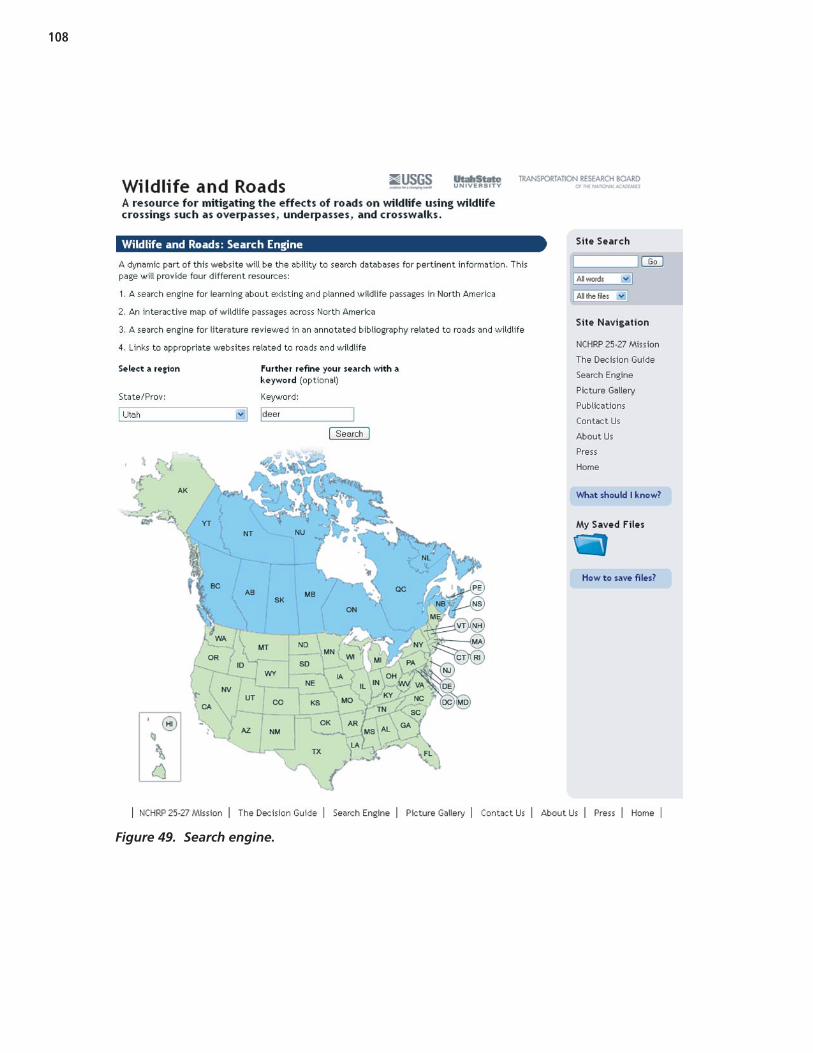
108

Figure 49. Search engine.

109

Figure 50. Example of the Decision Guide search engine results for Utah.

110

1. Adams, L.W., “Small Mammal Use of an Interstate Highway Me-dian Strip.” Journal of Applied Ecology, Vol. 21 (1984) pp. 175–178.

2. Adams, L.W. and Geis, A.D., “Effects of Roads on Small Mam-mals.” Journal of Applied Ecology, Vol. 20 (1983) pp. 403–415.

3. Addicott, J.F., Aho, J.M., Antolin, M.F., Padilla, D.K., Richardson,J.S. and Soluk, D.A., “Ecological Neighborhoods: Scaling Environ-mental Patterns.” Oikos, Vol. 49 (1987) pp. 340–346.

4. Allen, R.E. and McCullough, D.R., “Deer-Car Accidents in South-ern Michigan.” Journal of Wildlife Management, Vol. 40 (1976) pp.317–325.

5. Anderson, D.R., Burnaham, K.P., White, G.C. and Otis, D.L.,“Density Estimation of Small-Mammal Population Using a Trap-ping Web and Distance Sampling Methods.” Ecology, Vol. 64(1983) pp. 674–680.

6. Anonymous, “Comprehensive Wildlife Conservation Strategies.”State Progress Report #2, International Association of Fish andWildlife Agencies, Washington, DC (2004). URL: www.teamingwithwildlife.org/

7. Arcese, P., “Intrasexual Competition, Mating System, and NatalDispersal in Song Sparrows.” Animal Behaviour, Vol. 38 (1989)pp. 958–979.

8. Ashley, M. and Wills, C., “Analysis of Mitochondrial DNA Poly-morphisms Among Channel Island Deer Mice.” Evolution, Vol.41(1987) pp. 854–863.

9. Austin, J., Viani, K. and Hammond, F., “Vermont Wildlife Habi-tat Linkage Analysis.” Report to Vermont Agency of Transportation,VTrans Research Advisory Council No. RSCH008–967 (2006).

10. Baker, R.H., “Are Man-Made Barriers Influencing MammalianSpeciations?” Journal of Mammalogy, Vol. 79 (1998) pp. 370–371.

11. Bank, F., Irwin, L., Evink, G., Gray, M., Hagood, S., Kinar, J., Levey,A., Paulson, D., Ruediger, B., Sauvajot R., Scott, D., and White, P.,“Wildlife Habitat Connectivity Across European Highways.”FHWA Report PL-02-011, U.S. Department of Transportation,Federal Highway Administration, International TechnologyExchange Program (2002).

12. Barnett, J.L., How, R.A. and Humphreys, W.F., “The Use of Habi-tat Components by Small Mammals in Eastern Australia.” Aus-tralian Journal of Ecology, Vol. 3 (1978) pp. 277–85.

13. Barnum, S., “Preliminary Analysis of Locations Where WildlifeCrosses Highways in the Southern Rocky Mountains.” Interna-tional Conference on Ecology and Transportation, Keystone, CO,Proceedings (2001) pp. 565–573.

14. Barnum, S., “Identifying the Best Locations Along Highways toProvide Safe Crossing Opportunities for Wildlife.” CDOT Report

CDOT-DTD-UCD-2003-9, Colorado Department of Transporta-tion, Research Branch, Denver, CO (2003).

15. Bashore, T.L., Tzilkowski, W.M. and Bellis, E.D., “Analysis ofDeer-Vehicle Collision Sites in Pennsylvania.” Journal of WildlifeManagement, Vol. 49 (1985) pp. 769–774.

16. Bates, K., “Design of Road Culverts for Fish Passage.” WashingtonDepartment of Fish and Wildlife Report, Olympia, WA (2003).

17. Begon, M., Towsend, C.R. and Harper, J.L., Ecology – From Indiv-iduals to Ecosystems. Blackwell Publishing, Malden, MA (2006).738 pp.

18. Beier, P. and Barrett, R.H., “The Cougar in the Santa Ana Moun-tain Range, California.” Orange County Cooperative Final Report(1993).

19. Bellamy, P.E., Shore, R.F., Ardeshir, D., Treweek, J.R. and Sparks,T.H., “Road Verges as Habitat for Small Mammals in Britain.”Mammal Review, Vol. 30 (2000) pp. 131–139.

20. Bellis, E.D. and Graves, H.B., “Deer Mortality on a PennsylvaniaInterstate Highway.” Journal of Wildlife Management, Vol. 35(1971) pp. 232–237.

21. Benfield, F.K., Raimi, M. and Chen, D.D.T., Once There WereGreenfields. Natural Resources Defense Council, New York, NY(1999).

22. Bennetts, R.E., Nichols, J.D., Lebreton, J.D., Pradel, R., Hines, J.E.and Kitchens, W.M., “Methods for Estimating Dispersal Probabil-ities and Related Parameters Using Marked Animals.” Dispersal,Oxford University Press, NY (2001) pp. 3–17.

23. Beringer, J.J., Seibert, S.G. and Pelton, M.R., “Incidence of RoadCrossing by Black Bears on Pisgah National Forest, NorthCarolina.” International Conference on Bear Research and Manage-ment, Proceedings Vol. 8 (1990) pp. 85–92.

24. Beyer, H.L., Hawth’s Analysis Guides for ArcGIS. (2004) www.spatialecology.com/hguides.

25. Biggs, J., Sherwood, S., Michalak, S., Hansen, L. and Bare, C.,“Animal-Related Vehicle Accidents at the Los Alamos NationalLaboratory, New Mexico.” The Southwestern Naturalist, Vol. 49(2004) pp. 384–394.

26. Bissonette, J.A., “Scaling Roads and Wildlife: The CinderellaPrinciple.” Zeitschrift für Jagdwissenschaft (supplement), Vol. 48(2002) pp. 208–214.

27. Bissonette, J.A., “Linking Landscape Patterns to Biological Real-ity.” Landscape Theory and Resource Management: Linking Theoryto Practice, Island Press, Washington, D. C. (2003) pp. 15–34.

28. Bissonette, J.A. and Hammer, M., “Effectiveness of Earthen Re-turn Ramps in Reducing Big Game Highway Mortality in Utah.”

References

Report UT-01.09, Utah Department of Transportation, Salt LakeCity, UT (2000).

29. Bissonette, J.A. and Storch, I., “Fragmentation: Is the MessageClear?” Conservation Ecology, Vol. 6 (2002) p.14. [online]www.consecol.org/vol6/iss2/art14

30. Bissonette, J.A. and Storch, I., Landscape Theory and ResourceManagement: Linking Theory to Management. Island Press, Wash-ington, DC (2003).

31. Boarman, W.I., Sazaki, M. and Jennings, W.B., “The Effect ofRoads, Barrier Fences, and Culverts on Desert Tortoise Popula-tions in California, USA.” Conservation, Restoration, and Man-agement of Tortoises and Turtles—An International Conference,The New York Turtle and Tortoise Society, Proceedings (1997)pp. 54–58.

32. Boots, B.N. and Getis, A., Point Pattern Analysis. Sage Publica-tions, Beverly Hills, CA (1988).

33. Bowman, J., Jaeger, J.A.G. and Fahrig, L., “Dispersal Distance ofMammals is Proportional to Home Range Size.” Ecology, Vol. 83(2002) pp. 2049–2055.

34. Bowne, D. R. and Bowers, M. A., “Interpatch Movements in Spa-tially Structured Populations: A literature review.” Landscape Ecol-ogy, Vol. 19 (2004) pp. 1–20.

35. Braumandl, T.F., Curran, M.P., Davis, G.D., Quesnel, H.J.,Woods, G.P., DeLong, D.L. and Ketcheson, M.V., “BiogeoclimaticSubzones and Variants of the Nelson Forest Region.” A FieldGuide for Site Identification and Interpretation for the Nelson ForestRegion, Land Management Handbook 20, Ministry of Forests,Victoria, BC Canada (1992) pp. 44–199.

36. Brock, R.E. and Kelt, D.A., “Influence of Roads on the EndangeredStephens’ Kangaroo Rat (Dipodomys stephensi): Are Dirt andGravel Roads Different?” Biological Conservation, Vol. 118 (2004)pp. 633–640.

37. Brown, J.H., Macroecology. University of Chicago Press, Chicago,IL (1995).

38. Bullock, J.M., Kenward, R.E. and Hails, R., Dispersal Ecology.Blackwell Science, Oxford, England (2002).

39. Brzezinski, M., Jedrzejewski, W. and Jedrzejewska, B., “WinterHome Ranges and Movement of Polecats Mustela putorius inBialowieza Primeval Forest, Poland.” Acta Theriologica, Vol. 37(1992) pp. 181–191.

40. Buckland, S.T., Anderson, D.R., Burnham, K.P. and Laake, J.L.,Distance Sampling: Estimating Abundance of Biological Populations.Chapman and Hall, London, England (1993).

41. Buckland, S.T., Anderson, D.R., Burnham, K.P., Laake, J.L.,Borchers, D.L. and Thomas, L., Introduction to Distance Sampling.Oxford University Press, London, England (2001).

42. Buckland, S.T., Anderson, D.R., Burnham, K.P., Laake, J.L.,Borchers, D.L. and Thomas, L., Advanced Distance Sampling. Ox-ford University Press, New York, N.Y., USA (2004).

43. Burnett, S.E., “Effects of a Rainforest Road on Movements ofSmall Mammals: Mechanisms and Implications.” Wildlife Re-search, Vol.19 (1992) pp. 5–104.

44. Burt, W.H., “Territoriality and Home Range Concepts as Appliedto Mammals.” Journal of Mammalogy, Vol. 24 (1943) pp. 346–352.

45. Carbaugh, B., Vaughan, J.P., Bellis, E.D. and Graves, H.B.,“Distribution and Activity of White-Tailed Deer Along an Inter-state Highway.” Journal of Wildlife Management, Vol. 39 (1975)pp. 570–581.

46. Carr, M., Hoctor, T., Goodison, C., Zwick, P., Green, J., Hernan-dez, P., McCain, C., Teisinger, J., Whitney, K., “Southeastern Eco-logical Framework.” Final Report, Geoplan Center, Departmentsof Landscape Architecture, Urban and Regional Planning, and

Wildlife Ecology and Conservation, University of Florida,Gainesville, FL (2002).

47. Case, R.M., “Interstate Highway Road-killed Animals: A DataSource for Biologists.” Wildlife Society Bulletin, Vol. 6 (1978)pp. 8–13.

48. Cherry, S., “A Comparison of Confidence Interval Methods forHabitat Use-Availability Studies.” Journal of Wildlife Management,Vol. 60 (1996) pp. 653–658.

49. Clark, B.K., Clark, B.S., Johnson, L.A. and Hayne, M.T., “Influenceof Roads on Movements of Small Mammals.” Southwestern Natu-ralist, Vol. 46 (2001) pp. 338–344.

50. Clark, P.J. and Evans, F.C., “Distance to Nearest Neighbor as aMeasure of Spatial Relationships in Populations.” Ecology, Vol. 35(1954) pp. 445–453.

51. Clevenger, A.P., Chruszcz, B., and Gunson, K.E., “Highway Miti-gation Fencing Reduces Wildlife-Vehicle Collisions.” WildlifeSociety Bulletin, Vol. 29 (2001) pp. 646–653.

52. Clevenger, A.P., Chruszcz, B., and Gunson, K.E., “Spatial Patternsand Factors Influencing Small Vertebrate Fauna Road-Kill Aggrega-tions.” Biological Conservation, Vol. 109 (2003) pp. 15–26.

53. Clevenger, A.P., Chruszcz, B., Gunson, K. and Wierzchowski, J.,“Roads and Wildlife in the Canadian Rocky Mountain Parks—Movements, Mortality and Mitigation.” Final Report, ParksCanada, Banff, Alta, Canada (2002).

54. Clevenger, A.P., Purroy, F.J. and Campos, M.A., “Habitat Assess-ment of a Relict Brown Bear Ursus arctos Population in NorthernSpain.” Biological Conservation, Vol. 80 (1997) pp. 17–22.

55. Clevenger, A.P. and Waltho, N., “Dry Drainage Culvert Use andDesign Considerations for Small- and Medium-sized MammalMovement across a Major Transportation Corridor.” Interna-tional Conference on Wildlife Ecology and Transportation,Missoula, MT Proceedings (1999) pp. 263–277.

56. Clevenger, A.P. and Waltho, N., “Factors Influencing the Effec-tiveness of Wildlife Underpasses in Banff National Park, Alberta,Canada.” Conservation Biology, Vol. 14 (2000) pp. 47–56.

57. Clevenger, A.P. and Waltho, N., “Long-Term Year-Round Moni-toring of Wildlife Crossing Structures and the Importance ofTemporal and Spatial Variability in Performance Studies.” Interna-tional Conference on Ecology and Transportation, Lake Placid, NYProceedings (2003) pp. 293–302.

58. Clevenger, A.P. and Waltho, N., “Performance Indices to IdentifyAttributes of Highway Crossing Structures Facilitating Move-ments of Large Mammals.” Biological Conservation, Vol. 121(2005) pp. 453–464.

59. Clobert, J., Wolff, J.O., Nichols, J.D., Danchin, E. and Dhondt,A.A., “Introduction.” Dispersal, Oxford University Press, NY(2001) pp xvii-xxi.

60. Connelly, J.W., Knick, S.T., Schroeder, M.A. and Stiver, S.J., “Conser-vation Assessment of Greater Sage-Grouse and Sagebrush Habitats.”Unpublished report, Western Association of Fish and Wildlife Agen-cies, Cheyenne, WY (2004).

61. Conover, M.R., Pitt, W.C., Kessler, K.K., DuBow, T.J. and Sanborn,W.A., “Review of Human Injuries, Illnesses, and Economic LossesCaused by Wildlife in the United States.” Wildlife Society Bulletin,Vol. 23 (1995) pp. 407–414.

62. COST 341. 2006. URL: cordis.europa.eu/cost-transport/src/cost-341.htm.

63. Courtois, R., Labonte, J. and Ouelle, J.P., “Déplacements et Superfi-cie du Domaine Vital de l’Orignal, Alces alces, dans l’Est du Quebec.”Canadian-Field Naturalist, Vol. 112 (1998) pp. 602–610.

64. Covell, D.F., Miller, D.S. and Darasov, W.H., “Cost of Locomo-tion and Daily Energy Expenditure by Free-Living Swift Foxes

111

(Vulpes velox): A Seasonal Comparison.” Canadian Journal of Zo-ology, Vol. 74 (1996) pp. 283–290.

65. Craighead, A.C., Craighead, F.L. and Roberts, E.A., “BozemanPass Wildlife Linkage and Highway Safety Guide.” InternationalConference on Ecology and Transportation, Keystone, CO, Pro-ceedings (2001) pp 405–412.

66. Cramer, P.C. and Bissonette, J.A., “Wildlife Crossings in NorthAmerica: The State of the Science and Practice.” InternationalConference on Ecology and Transportation, San Diego, CA, Pro-ceedings (2006) pp. 442–447.

67. Cressie, N., Statistics for Spatial Data. John Wiley and Sons, NewYork, N.Y. (1991).

68. Damuth, J., “Population Density and Body Size in Mammals.”Nature, Vol. 290 (1981) pp. 699–700.

69. Davidson, D., “Innovative Partnerships that Address Highway Im-pacts to Wildlife Habitat Connectivity in the Northern Rockies.”International Conference on Ecology and Transportation, LakePlacid, NY, Proceedings (2003) pp. 195–203.

70. Dillman, D.A., Mail and Internet Surveys: The Tailored DesignMethod. John Wiley and Sons, Inc., New York, NY (2000).

71. Dodd, C.K., Barichivich, W.J. and Smith, L.L., “Effectiveness of aBarrier Wall and Culverts in Reducing Wildlife Mortality on aHeavily Traveled Highway in Florida.” Biological Conservation,Vol. 118 (2004) pp. 619–631.

72. Dodd, N. L., “Characteristics of Elk-Vehicle Collisions and Com-parison to GPS-Determined Highway Crossing Patterns.” Inter-national Conference on Ecology and Transportation, San Diego,CA, Proceedings (2006) pp. 461–477.

73. Dodd, N.L., Gagnon, J. and Schweinsburg, R., “Evaluation ofMeasures to Minimize Wildlife-Vehicle Collisions and MaintainWildlife Permeability Across Highways.” Quarterly Progress Report10, Submitted to the Research Technical Advisory Committeeand Project Implementation Working Group, Arizona Game andFish Department, Research Branch, Phoenix, AZ (2004).

74. Dodd, N.L., Gagnon, J.W. and Schweinsburg, R.E., “Phases II andIII: Evaluation of Measures to Minimize Wildlife-Vehicle Colli-sions and Maintain Wildlife Permeability Across Highways.”Progress Report, Arizona Game and Fish Department (2006).

75. Doerr, E.D. and Doerr, V.A.J., “Dispersal Range Analysis: Quan-tifying Individual Variation in Dispersal Behaviour.” Oecologia,Vol. 142 (2005) pp. 1–10.

76. Endries, M., Gilbert, T. and Kautz, R., “Environmental Planning inFlorida: Mapping Wildlife Needs in Florida: The Integrated WildlifeHabitat Ranking System.” International Conference on Ecology andTransportation, Lake Placid, NY, Proceedings (2003) pp. 525–533.

77. Environmental Systems Research Institute, ArcView GIS Version3.3., Redlands, CA (1999).

78. Environmental Systems Research Institute, ArcGIS Version 9.0,Redlands, CA (2003).

79. Evink, G., NCHRP Synthesis of Highway Practice 305: InteractionBetween Roadways and Wildlife Ecology. Transportation ResearchBoard of the National Academies, Washington, DC (2002).

80. Evink, G., “Wetlands, Wildlife, and Ecosystems.” EnvironmentalResearch Needs in Transportation Conference, TransportationResearch Board, Washington, DC (2002).

81. Fahrig, L., Pedlar, J.H., Pope, S.E., Taylor, P.D. and Wegner, J.F.,“Effect of Road Traffic on Amphibian Density.” Biological Conser-vation, Vol. 74 (1995) pp. 177–182.

82. Farrell, J.E., Irby, L.R. and McGowen, P.T., “Strategies for Ungu-late Vehicle Collision Mitigation.” Intermountain Journal of Sci-ence, Vol. 8 (2002) pp. 1–18.

83. Federal Highway Administration, “America’s Highways1776–1976: A History of the Federal Aid Program.” U.S. Depart-ment of Transportation Report, Washington, DC (1979).

84. Federal Highway Administration, “Highway Statistics 2002: Road-way Extent, Characteristics and Performance.” U.S. Department ofTransportation Report, Washington, DC (2002).

85. Federal Highway Administration, “Keeping it Simple: Easy Waysto Help Wildlife Along Roads.” (2006). URL: www.fhwa.dot.gov/environment/wildlifeprotection/index.cfm

86. Feldhammer, G.A., Gates, J.E., Harman, D.M., Loranger, A.J. andDixon, K.R., “Effects of Interstate Highway Fencing on White-Tailed Deer Activity.” Journal of Wildlife Management, Vol. 50(1986) pp. 497–503.

87. Ferreras, P., Aldama, J.J., Beltran, J.F. and Delibers, M., “Rates andCauses of Mortality in a Fragmented Population of Iberian LynxFelis pardini Temminck, 1824.” Biological Conservation, Vol. 61(1992) pp. 197–202.

88. Finder, R.A., “Relationships between Landscape Patterns andWhite-Tailed Deer/Vehicle Accidents.” Master’s Thesis, SouthernIllinois University-Carbondale, IL (1997).

89. Finder, R.A., Roseberry, J.L. and Woolf, A., “Site and LandscapeConditions at White-Tailed Deer-Vehicle Collision Locations inIllinois.” Landscape and Urban Planning, Vol. 44 (1999) pp. 77–85.

90. Findlay, C.S. and Houlahan, J., “Anthropogenic Correlates ofSpecies Richness in Southeastern Ontario Wetlands.” ConservationBiology, Vol. 11 (1997) pp. 1000–1009.

91. Fletcher, D.R., Summary of a Workshop. Conference Proceedingson the Web 1: Environmental Spatial Information for Transporta-tion: A Peer Exchange on Partnerships. Transportation ResearchBoard of the National Academies, Washington, DC (2004). URL:http://www.trb.org/news/blurb_detail.asp?id=3956

92. Florida Fish and Wildlife Commission, “Integrated Wildlife Habi-tat Ranking System.” GIS data, on compact disc, Florida Fish andWildlife Commission, Tallahassee, FL (2004).

93. Foresman, K., “Monitoring Animal Use of Modified DrainageCulverts on the South Lolo Project.” Report FHWA/MT-01-004/8117–15, Prepared for the State of Montana in cooperationwith the U.S. Department of Transportation, Federal HighwayAdministration, Missoula, MT (2001).

94. Foresman, K., “Small Mammal Use of Modified Culverts on theLolo South Project of Western Montana—an Update.” Interna-tional Conference on Ecology and Transportation, Lake Placid,NY, Proceedings (2003) pp. 342–343.

95. Forman, R.T.T. and Alexander, L.E., “Roads and Their Major Eco-logical Effects.” Annual Review of Ecology and Systematics, Vol. 29(1998) pp. 207–231.

96. Forman, R.T., Friedman, D.S., Fitzhenry, D., Martin, J.D., Chen, A.S.and Alexander, L.E., “Ecological Effects of Roads: Toward ThreeSummary Indices and an Overview for North America.” HabitatFragmentation & Infrastructure, Delft, Netherlands, Ministry ofTransport, Public Works and Water Management (1997) pp. 40–54.

97. Forman, R.T., Reineking, B., and Hersperger, A.M., “Road Trafficand Nearby Grassland Bird Patterns in a Suburbanizing Land-scape.” Environmental Management, Vol. 29 (2002) pp. 782–800.

98. Forman, R.T., Sperling, D., Bissonette, J.A., Clevenger, A.P.,Cutshall, C.D., Dale, V.H., Fahrig, L., France, R., Goldman, C.R.,Heanue, K., Jones, J.A., Swanson, F.J., Turrentine, T. and Winter,T.C., Road Ecology: Science and Solutions. Island Press, Washing-ton, DC (2003).

99. Foster, M. and Humphrey, S., “Effectiveness of Wildlife Crossingsin Reducing Animal Auto Collisions on Interstate 75, Big Cypress

112

Swamp, Florida.” Florida Department of Transportation and Uni-versity of Florida Report, Gainesville, FL (1992).

100. Foster, M. and Humphrey, S., “Use of Highway Underpasses byFlorida Panthers and Other Wildlife.” Wildlife Society Bulletin,Vol. 23 (1995) pp. 95–100.

101. Fuller,T., “Population Dynamics of Wolves in North-central Min-nesota.” Wildlife Monographs, Vol. 105 (1989) pp. 1–41.

102. Gagnon, J., Dodd, N.L. and Manzo, A.L., “Use of Video Surveil-lance to Assess Wildlife Behavior and Use of Wildlife Underpassesin Arizona.” International Conference on Ecology and Trans-portation, San Diego, CA, Proceedings (2006) pp. 534–544.

103. Gerlach, G. and Musolf, K., “Fragmentation of Landscapes as aCause for Genetic Subdivision in Bank Voles.” Conservation Biol-ogy, Vol. 14 (2000) pp. 1066–1074.

104. Getis, A. and Franklin, J., “Second-Order Neighborhood Analysisof Mapped Point Patterns.” Ecology, Vol. 68 (1987) pp. 473–477.

105. Gibeau, M.L., “A Conservation Biology Approach to Managementof Grizzly Bears in Banff National Park, Alberta.” Ph.D. thesis,University of Calgary, Calgary, AB (2000) 129 pp.

106. Gibeau, M.L. and Herrero, S., “Roads, Rails and Grizzly Bears inthe Bow River Valley, Alberta.” International Conference onWildlife Ecology and Transportation, Fort Meyers, FL, Proceed-ings (1998) pp. 104–108.

107. Goosem, M., “Effects of Tropical Rainforest Roads on SmallMammals: Inhibition of Crossing Movements.” Wildlife Research,Vol. 28 (2001) pp. 351–364.

108. Griffith, M.S. and Council, F.M., “The Highway Safety Informa-tion System: United States Department of Transportation Multi-State Safety Analysis Database.” Traffic Safety on Two ContinentsConference Proceedings, Malmo, Sweden (2000).

109. Gunther, K., Biel, M.J. and Robison, H.L., “Influence of VehicleSpeed and Vegetation Cover Type on Road-killed Wildlife inYellowstone National Park.” Wildlife and Highways: SeekingSolutions to an Ecological and Socio-Economic Dilemma, TheSeventh Annual Meeting of The Wildlife Society Proceedings,Nashville, TN, (2000).

110. Hansen, A.J., Rasker, R., Maxwell, B., Rotella, J.J., Johnson, J.D.,Parmenter, A.W., Langner, U., Cohen, W.B., Lawrence, R.L. andKraska, M.P.V., “Ecological Causes and Consequences of Demo-graphic Change in the New West.” BioScience, Vol. 52 (2002) pp.151–162.

111. Hardy, A., Clevenger, A.P., Huijser, M. and Neale, G., “AnOverview of Methods and Approaches for Evaluating the Effec-tiveness of Wildlife Crossing Structures: Emphasizing the Sciencein Applied Science.” International Conference on Ecology andTransportation, Lake Placid, NY, Proceedings (2003) pp. 319–330.

112. Harestad, A.S. and Bunnell, F.L., “Home Range and BodyWeight—A Reevaluation.” Ecology, Vol. 60 (1979) pp. 389–402.

113. Harwood, D., Council F., Hauer, E., Hughes W. and Vogt, A.,“Prediction of the Expected Safety Performance of Rural Two-Lane Highways”. FHWA Report FHWA-RD-99-207, Federal High-way Administration, Washington, DC (2000).

114. Hauer, E., Observational Before-After Studies in Road Safety: Esti-mating the Effect of Highway and Traffic Engineering Measures onRoad Safety. Pergamon Press, Elsevier Science Ltd, Oxford, Eng-land (1997).

115. Hawbaker, T.J. and Radeloff, V.C., “Roads and Landscape Patternin Northern Wisconsin Based on a Comparison of Four RoadData Sources.” Conservation Biology, Vol. 18 (2004) pp. 123–125.

116. Hedlund, J.H., Curtis, P.D., Curtis, G. and Williams, A.F., “Meth-ods to Reduce Traffic Crashes Involving Deer: What Works and

What Does Not.” Insurance Institute for Highway Safety Report,Arlington, VA (2003).

117. Hengeveld, R., “Small Step Invasion Research.” Trends in Ecologyand Evolution, Vol. 9 (1994) pp. 339–342.

118. Hewitt, D.G., Cain, A., Tuovila, V., Shindle, D.B. and Tewes,M.E., “Impacts of an Expanded Highway on Ocelots and Bobcats in Southern Texas and Their Preferences for High-way Crossings.” International Conference on Wildlife Ecologyand Transportation, Ft. Meyers, FL, Proceedings (1998) pp.126–134.

119. Heydecker, B.J. and Wu, J., “Using the Information in Road CrashRecords.” 19th Petroleum Technology Research Centre SummerAnnual Meeting, London, England, Proceedings (1991).

120. Hjeljord, O., “Dispersal and Migration in Northern Forest Deer—Are There Unifying Concepts?” Alces, Vol. 37 (2001) pp. 353–370.

121. Holland, W.D. and Coen, G.M., “Ecological Land Classification ofBanff and Jasper National Parks.” The Wildlife Inventory ReportVolume III, Canadian Wildlife Service, Edmonton, AB (1983).

122. Holling, C.S., “Cross-Scale Morphology, Geometry, and Dynam-ics of Ecosystems.” Ecological Monographs, Vol. 62 (1992) pp.447–502.

123. Hosmer, D.W. and Lemeshow, S., Applied Logistic Regression. JohnWiley and Sons, NY (1989).

124. Hubbard, M.W., Danielson, B.J. and Schmitz, R.A., “Factors In-fluencing the Location of Deer-Vehicle Accidents in Iowa.” Jour-nal of Wildlife Management, Vol. 64 (2000) pp. 707–713.

125. Huijser, M.P., Gunson, K.E. and Abrams, C., “Wildlife-VehicleCollisions and Habitat Connectivity Along Montana Highway 83in the Seeley-Swan Valley, Montana: A Reconnaissance.” WesternTransportation Institute Report No. FHWA/MT-05-009/8177,Montana State University, Bozeman, MT (2006).

126. Huijser, M.P., Galarus, D.E. and Hardy, A., “Software for PocketPC to Collect Road-Kill Data.” International Conference onEcology and Transportation, San Diego, CA, Proceedings (2006)p. 640.

127. International Conference on Ecology and Transportation: A Timefor Action, Keystone, CO, Proceedings (2001).

128. International Conference on Ecology and Transportation: Mak-ing Connections, Lake Placid, NY, Proceedings (2003).

129. Iuell, B., Bekker, C.J., Cuperus, R., Dufek, J., Fry, G., Hicks, C.,Hlavac, V., Keller, V., Rosell, C., Sangwine, T., Torslov, N. andWandall, B., Wildlife and Traffic: A European Handbook for Identi-fying Conflicts and Designing Solutions. KNNV Publishers, Brussels,Belgium (2003).

130. Jackson, S.D., “Proposed Design and Considerations for Use ofAmphibian and Reptile Tunnels in New England.” University ofMassachusetts Report, Amherst, MA (2003) URL: www.umass.edu/nrec/onlinedocs.html.

131. Jackson, S.D. and Tyning, T.F., “Effectiveness of Drift Fences andTunnels for Moving Spotted Salamanders Ambystoma maculatumUnder Roads.” Amphibians and Roads, The Toad Tunnel Confer-ence, ACO Polymer Products, Shefford, England, Proceedings(1989) pp. 93–99.

132. Jaeger, J.A.G., “Landscape Division, Splitting Index, and EffectiveMesh Size: New Measures of Landscape Fragmentation.” Land-scape Ecology, Vol. 15 (2000) pp. 115–130.

133. Jaeger, J.A.G., Bowman, J., Brennan, J., Fahrig, L., Bert, D.,Bouchard, J., Charbonneau, N., Frank, K., Gruber, B. and VonToschanowitz, K., “Predicting When Animal Populations Are atRisk from Roads: An Interactive Model of Road AvoidanceBehavior.” Ecological Modeling, Vol. 185 (2005) pp. 329:348.

113

134. Joyce, T.L. and Mahoney, S.P., “Spatial and Temporal Distribu-tions of Moose-Vehicle Collisions in Newfoundland.” WildlifeSociety Bulletin, Vol. 29 (2001) pp. 281–291.

135. Kaseloo, P.A. and Tyson, K.O., “Synthesis of Noise Effects onWildlife Populations.” Report Prepared for U.S. Department ofTransportation, Federal Highway Administration, McLean, VA(2004).

136. Kassar, C. and Bissonette, J.A., “Deer-Vehicle Crash Hotspots inUtah: Data for Effective Mitigation.” UTCFWRU Project ReportNo. 2005(1): 1–128, Utah Cooperative Fish and Wildlife ResearchUnit, Utah State University, Logan, UT (2005).

137. Kattan, G., Hernandez, O.L., Goldstein, I., Rojas, V., Murillo, O.,Gomez, C., Restrepo, H. and Cuesta, F., “Range Fragmentation inthe Spectacled Bear Tremarctos ornatus in the Northern Andes.”Oryx, Vol. 38 (2004) pp. 155–163.

138. Keller, I., Largiader, C.R. and Nentwig, W., “Recent FragmentationDue to Major Roads Leads to a Reduction of Gene Flow in GroundBeetles.” International Conference on Habitat Fragmentation dueto Transportation Infrastructure, Brussels, Belgium, Proceedings(2003).

139. Kelt, D.A. and Van Vuren, D.H., “The Ecology and Macroecologyof Mammalian Home Range Area.” American Naturalist, Vol. 157(2001) pp. 637–645.

140. Kintsch, J., “Linking Colorado’s Landscapes.” InternationalConference on Ecology and Transportation, San Diego, CA, Pro-ceedings (2006) pp. 138–142.

141. Kleiber, M., The Fire of Life: An Introduction to Animal Energetics.John Wiley and Sons, Hoboken, NJ (1961).

142. Knapp, K. Pooled fund proposal (2004). URL: www.pooledfund.org/documents/solicitations/906.pdf

143. Kozell, R.M. and Fleharty, E.D., “Movements of Rodents AcrossRoads.” Southwestern Naturalist, Vol. 24 (1979) pp. 239–248.

144. Lemel, J., Truve, J. and Soderberg, B., “Variation in Ranging andActivity Behaviour of European Wild Boar Sus scrofa in Sweden.”Wildlife Biology, Vol 9, Supplement 1 (2003) pp. 29–36.

145. Levine, N., CrimeStat: A Spatial Statistics Program for the Analysisof Crime Incident Locations. Ned Levine and Associates, Annandale,VA and National Institute of Justice, Washington, DC (1999).

146. Levine, N., CrimeStat III: A Spatial Statistics Program for the Analy-sis of Crime Incident Locations. Ned Levine and Associates, Houston,TX and the National Institute of Justice, Washington, DC (2004).

147. Lindstedt, S.L, Miller, B.J. and Buskirk, S.W., “Home Range, Time,and Body Size in Mammals.” Ecology, Vol. 67 (1986) pp. 413–418.

148. Lloyd, J. and Casey, A., “Wildlife Hotspots Along Highways inNorthwestern Oregon.” Report to Oregon Department of Trans-portation, Portland, OR (2005).

149. Little, S.J., Harcourt, R.G. and Clevenger, A.P.,”Do Wildlife Pas-sages Act as Prey Traps?” Biological Conservation, Vol. 107 (2002)pp. 135–145.

150. Lotz, M.A., Land, E.D. and Johnson, K.G., “Evaluation of StateRoad 29 Wildlife Crossings.” Final Report to the Florida Game andFresh Water Fish Commission, Tallahassee, FL (1996).

151. Lyon, A.G. and Anderson, S.H., “Potential Gas Development Im-pacts on Sage Grouse Nest Initiation and Movement.” WildlifeSociety Bulletin, Vol. 31 (2003) pp. 486–491.

152. MacDonald, L.A. and Smith, S., “Bridge Replacements: AnOpportunity to Improve Habitat Connectivity.” InternationalConference on Wildlife Ecology and Transportation, Missoula,MT, Proceedings (1999).

153. Mader, H.J., “Animal Habitat Isolation by Roads and AgriculturalFields.” Biological Conservation, Vol. 29 (1984) pp. 81–96.

154. Mader, H.J., Schell, C. and Kornacker, P., “Linear Barriers toArthropod Movements in the Landscape.” Biological Conservation,Vol. 54 (1990) pp. 209–222.

155. Maehr, D.S., Land, E.D. and Roelke, M.E., “Mortality Patterns ofPanthers in Southwest Florida.” Annual Conference of the South-eastern Association Fish and Wildlife Agencies, Proceedings Vol.45 (1991) pp. 201–207.

156. Maine Department of Transportation, “Collisions BetweenWildlife Species and Motor Vehicles in Maine 1997–2001.” Traf-fic Engineering Division Report, Bureau of Maintenance andOperations, Maine Department of Transportation, Augusta, ME(2002).

157. Maine Department of Transportation, “Fish Passage Policy andDesign Guide.” Maine Department of Transportation Report, Envi-ronmental Office, Augusta, ME (2004). URL: mainegov-images.informe.org/mdot/environmental-office-homepage/documents/FISH%20PASSAGE%20POLICY%20AND%20DESIGN%20GUIDE%202nd%20Ed%202004.pdf

158. Malo, J.E., Suarez, F. and Diez, A., “Can We Mitigate Wildlife-Vehicle Accidents Using Predictive Models?” Journal of AppliedEcology, Vol. 41 (2004) pp. 701–710.

159. Mansfield, T.M. and Miller, B.D., “Highway Deer-Kill District 02Regional Study.” Caltrans Internal Report, Sacramento, CA (1975).

160. McCaffrey, K.R., “Road-Kills Show Trends in Wisconsin DeerPopulations.” Journal of Wildlife Management, Vol. 37 (1973) pp.212–216.

161. McCune, B. and Grace, J. B., Analysis of Ecological Communities.MjM Software Design, ISBN 0-9721290-0-6, Gleneden Beach, OR(2002).

162. McCune, B. and Mefford, M.J., PC-ORD: Multivariate Analysis ofEcological Data. Version 4.36, MjM Software, Gleneden Beach,OR, (1999).

163. McGuire, T., “Connecting Values, Process, and Project Design:Twinning the Trans-Canada Highway in Banff National Park inCanada.” International Conference on Ecology and Transporta-tion, San Diego, CA, Proceedings (2006) p.77

164. McIninch, S.P. and Garman, G.C., “Strategies for ImpedimentRehabilitation to Create Fish Passage Opportunities in the Rappa-hannock River Basin.” Report VTRC 04-CR2, Submitted to theVirginia Transportation Research Council, Virginia Common-wealth University, Richmond, VA (2004).

165. McNab, B.K., “Bioenergetics and the Determination ofHome Range Size.” American Naturalist, Vol. 97 (1963)pp. 133–140.

166. Mech, L.D., Fritts, S.H., Raddle, G.L. and Paul, W.J., “Wolf Distri-bution and Road Density in Minnesota.” Wildlife Society Bulletin,Vol. 16 (1988) pp. 85–87.

167. Menard, S., “Applied Logistic Regression Analysis,” Sage Univer-sity Paper Series Report 07–106, Sage Publications, Thousand Oaks,CA (1995).

168. Merriam, G., “Important Concepts from Landscape Ecology forGame Biologists.” Gibier Faune Sauvage, Vol 15 (1998)pp. 525–531.

169. Meyer, E. and Ahmed, I., “Modeling of Deer-Vehicle Crash Likeli-hood Using Roadway and Roadside Characteristics.” TransportationResearch Board Annual Meeting, Washington, DC Proceedings(2004) CD-ROM.

170. Mills, S.L. and Conrey, R.Y., “Highways as Potential Barriers toMovement and Genetic Exchange in Small Mammals.” FinalReport to Montana Department of Transportation, University ofMontana, School of Forestry, Missoula, MT (2003).

114

171. Mladenoff, D.J., Sickley, T.A., Haight, R.G. and Wydeven, A.P., “ARegional Landscape Analysis and Prediction of Favorable GrayWolf Habitat in the Northern Great Lakes Region.” ConservationBiology, Vol. 9 (1995) pp. 279–294.

172. Mladenoff, D.J., Sickley, T.A. and Wydeven, A.P., “PredictingGray Wolf Landscape Recolonization: Logistic Regression Mod-els vs. New Field Data.” Ecological Applications, Vol. 9 (1999)pp. 37–44.

173. Moa, P., Negard, A., Overskaug, K. and Kvam, T., “Possible Effectsof the Capture Event on Subsequent Space Use by Eurasian Lynx.”Wildlife Society Bulletin, Vol. 29 (2001) pp. 86–90.

174. Mohr, C.O., “Comparative Populations of Game, Fur, and OtherMammals.” American Midland Naturalist, Vol. 24 (1940)pp. 581–584.

175. Mohr, C.O., “Table of Equivalent Populations of North AmericanMammals.” American Midland Naturalist, Vol. 37 (1947) pp.223–249.

176. Morrison, M.L., Marcot, B.G. and Mannan, R.W., Wildlife-Habitat Relationships. University of Wisconsin Press, Madison,WI (1992).

177. Mysterud, A., “Temporal Variation in the Number of Car-KilledRed Deer Cervus elaphus in Norway.” Wildlife Biology, Vol. 10(2004) pp. 203–211.

178. Nagorsen, D.W., “Rodents and Lagomorphs of British Columbia.”Mammals of British Columbia, Vol. 4, Royal British ColumbiaMuseum, Victoria, BC Canada (2005).

179. Nathan, R., “Dispersal Biogeography.” Encyclopedia of Biodiver-sity, Academic Press, San Diego CA (2001) pp. 127–152.

180. Nathan, R., Perry, G., Cronin, J.T., Strand, A.E. and Cain, M.L.,“Methods for Estimating Long-Distance Dispersal.” Oikos, Vol.103 (2003) pp. 261–273.

181. National Research Council, Assessing and Managing the EcologicalImpacts of Paved Roads. National Research Council of the NationalAcademies, Committee on Ecological Impact of Road Density,Board of Environmental Studies and Toxicology, Division ofEarth and Life Studies, The National Academies Press, Washing-ton, DC (2006).

182. Neigel, J.E. and Avise, J.C., “Application of a Random Walk toGeographic Distributions of Animal Mitochondrial DNA Varia-tion.” Genetics, Vol. 135 (1993) pp. 1209–1220.

183. Nielsen, C.K., Anderson, R.G. and Grund, M.D., “Landscape Influ-ences on Deer-Vehicle Accident Areas in an Urban Environment.”Journal of Wildlife Management, Vol. 67 (2003) pp. 46–51.

184. Noss, R.F., “Landscape Connectivity: Different Functions at Dif-ferent Scales.” Landscape Linkages and Biodiversity, IslandPress,Washington, DC (1991) pp. 27–39.

185. O’Driscoll, R.L., “Descriptions of Spatial Pattern in Seabird Dis-tributions Along Line Transects Using Neighbour K Statistics.”Marine Ecology Progress Series, Vol. 165 (1998) pp. 81–94.

186. Oxley, D.J., Fenton, M.B. and Carmody, G.R., “The Effects ofRoads on Populations of Small Mammals.” Journal of AppliedEcology, Vol. 11(1974) pp. 51–59.

187. Penrod, K., Hunter, R. and Merrifield, M., “Missing Linkages:Restoring Connectivity to the California Landscape.” ConferenceCo-Sponsored by California Wilderness Coalition, The Nature Con-servancy, U.S. Geological Survey, Center for Reproduction of En-dangered Species, and California State Parks, Proceedings (2001).

188. Poll, D.M., Porter, M.M., Holroyd, G.L., Wershler, R.M. andGyug, L.W., “Ecological Land Classification of Kootenay NationalPark.” Wildlife Resource, Vol. II, Canadian Wildlife Service,Edmonton, AB Canada (1984).

189. Proctor, M.F., McLeleean, B.N. and Strobeck, C., “PopulationFragmentation of Grizzly Bears in Southeastern British Columbia,Canada.” Ursus, Vol. 13 (2002) pp. 153–160.

190. Puglisi, M.J., Lindzey, J.S. and Bellis, E.D., “Factors Associatedwith Highway Mortality of White-Tailed Deer.” Journal of WildlifeManagement, Vol. 38 (1974) pp. 799–807.

191. Putman, R.J., “Deer and Road Traffic Accidents: Options forManagement.” Journal of Environmental Management, Vol. 51(1997) pp. 43–57.

192. Ramp, D., Caldwell, J., Edwards, K., Warton, D. and Croft, D.,“Modelling of Wildlife Fatality Hotspots Along the Snowy MountainHighway in New South Wales, Australia.” Biological Conservation,Vol. 126 (2005) pp. 474–490.

193. Ramp, D., Wilson, V. and Croft, D., “Assessing the Impacts ofRoads in Peri-Urban Reserves: Road-Based Fatalities and RoadUsage by Wildlife in the Royal National Park, New South Wales,Australia.” Biological Conservation, Vol. 129 (2006) pp. 348–359.

194. Reed, D.F., Pojar, T.M. and Woodard, T.N., “Use of One WayGates by Mule Deer.” Journal of Wildlife Management, Vol. 38(1974) pp. 9–15.

195. Reed, D.,Woodward, T. and Pojar, T., “Behavioral Response ofMule Deer to a Highway Underpass.” Journal of Wildlife Manage-ment, Vol. 39 (1975) pp. 361–367.

196. Reeve, A.F., “Vehicle-Related Mortality of Mule Deer in NuggetCanyon, Wyoming.” Wyoming Cooperative Fisheries and WildlifeResearch Unit Report, Laramie, WY (1988).

197. Rei, W. and Seiz, A., “The Influence of Land Use on the GeneticStructure of Populations of the Common Frog Rana temporaria.”Biological Conservation, Vol. 54 (1990) pp. 239–249.

198. Renzhu, P., Zhang, M., Jialong, T. and Piao, C., “A Study of WinterMovement Characteristics for Wolverines in Daxinganling Moun-tains of China.” Acta Theriologica Sinica, Vol.15 (1995) pp. 209–214.

199. Rheindt, F.E., “The Impacts of Road on Birds: Does Song Fre-quency Play a Role in Susceptibility to Noise Pollution?” Journalof Ornithology, Vol. 144 (2003) pp. 295–306.

200. Ripley, B.D., Spatial Statistics. John Wiley and Sons, Hoboken, NJ(1981).

201. Romin, L.A. and Bissonette, J.A., “Deer-Vehicle Collisions: Statusof State Monitoring Activities and Mitigation Efforts.” WildlifeSociety Bulletin, Vol. 24 (1996) pp. 276–283.

202. Roof, J. and Wooding, J., “Evaluation of S.R. 46 Wildlife Cross-ing.” Florida Department of Transportation and the Florida Gameand Fresh Water Fish Commission Technical Report # 54, Tallahas-see, FL (1996).

203. Rosell, C., “Measures Applied to Mitigate Habitat Fragmentationin Spain.” International Conference on Ecology and Transporta-tion, Lake Placid, NY, Proceedings (2003) p.204.

204. Ruediger, B. and Lloyd, J., “A Rapid Assessment Process forDetermining Potential Wildlife, Fish and Plant Linkages for High-ways.” International Conference on Ecology and Transportation,Lake Placid, NY, Proceedings (2003) pp. 205–222.

205. Ruediger, B., Basting, P., Becker, D., Bustick, J., Cavill, P., Claar, J.,Foresman, K., Hieinz, G., Kaley, D., Kratville, S., Lloyd, J., Lucas,M., McDonald, S., Stockstad, G., Vore, J., Wall, K. and Wall, R.,“An Assessment of Wildlife and Fish Linkages on Highway 93—Western Montana.” Forest Service Publications #R1-04-81, USDAForest Service, USDI Fish and Wildlife Service, confederated Salishand Kootenai Tribe, Rocky Mountain Elk Foundation, MontanaFish, Wildlife and Parks, Montana Department of Transportation,Geodata Services, The University of Montana, Missoula, MT(2004) 41 pp.

115

206. Saeki, M. and. Macdonald, D.W., “The Effects of Traffic on theRaccoon Dog (Nyctereutes procyonoides viverrinus) and OtherMammals in Japan.” Biological Conservation, Vol. 118 (2004) pp.559–571.

207. Schmidt, N.M., Berg, T.B. and Jensen, T.S., “The Influence ofBody Mass on Daily Movement Patterns and Home Ranges of theCollared Lemming (Dicrostonyx groenlandicus).” Canadian Jour-nal of Zoology, Vol. 80 (2002) pp. 64–69.

208. Seiler, A., “Spatial Models to Predict Moose-Vehicle Collisions inSweden.” PhD Thesis, Department of Conservation Biology, SwedishUniversity of Agricultural Sciences, Uppsala, Sweden (2003).

209. Seton, E.T., Life Histories of Northern Animals: An Account ofMammals in Manitoba. Scribner and Sons, New York, NY (1909).

210. Sherwood, B., Cutler, D. and Burton, J.A. Wildlife and Roads: TheEcological Impact. Imperial College Press, London, England (2002).

211. Sielecki, L., “WARS Wildlife Accident Reporting System 2000 An-nual Report (1991–2000 Synopsis).” Environmental ManagementSection Report, Engineering Branch, British Columbia Ministry ofTransportation, Victoria BC Canada (2001).

212. Singleton, P., Gaines,W. and Lehmkuhl, J., “Landscape Perme-ability for Large Carnivores in Washington: A Geographic Infor-mation System Weighted-Distance and Least-Cost CorridorAssessment.” USDA Research Paper PNW-RP-549, PacificNorthwest Research Station, U.S. Forest Service, Portland, OR(2002).

213. Singleton, P.H. and Lehmkuhl, J.F., “Assessing Wildlife HabitatConnectivity in the Interstate 90 Snoqualmie Pass Corridor,Washington.” International Conference on Wildlife Ecology andTransportation, Missoula, MT, Proceedings (1999) pp. 75–84.

214. Singleton, P.H. and Lehmkuhl, J.F., “I-90 Snoqualmie PassWildlife Habitat Linkage Assessment.” USDA Forest Service ReportWA-RD 489.1., Washington State Department of Transportation,Olympia WA (2000).

215. Smith, D.J., Harris, L.D. and Mazzotti, F.J., “Highway-Wildlife Re-lationships: Development of a Decision-based Wildlife UnderpassRoad Project Prioritization Model on GIS Statewide Application.”Final Report to the Florida Department of Transportation, ContractNo. B-9943, University of Florida, Gainesville, FL (1998).

216. Snaith, T.V. and Beazley, K.F., “The Distribution, Status andHabitat Associations of Moose in Mainland Nova Scotia.” Pro-ceedings of the Nova Scotian Institute of Science, Vol. 42 (2004) pp.263–317.

217. Spellerberg, I.F. Ecological Effects of Roads. Science Publishers, Inc.,Enfield, NH (2002).

218. Spitz, F. and Janeau, G., “Spatial Strategies: An Attempt to Clas-sify Daily Movements of Wild Boar.” Acta Theriologica, Vol. 35(1990) pp. 139–149.

219. Sprent, P., Applied Nonparametric Statistical Methods. Chapmanand Hall, First edition, Stamford CT (1989) 259 pp.

220. SPSS, SPSS version 11.0 for Windows. SPSS Inc., Chicago, IL(2004).

221. SPSS, SPSS version 11.0.1 for Windows. SPSS Inc., Chicago, IL(2006).

222. Steen, D.A. and Gibbs, J.P., “Effects of Roads on the Structure ofFreshwater Turtle Populations.” Conservation Biology, Vol. 18(2004) pp. 1143–1149.

223. Stenseth, N.C. and Lidicker, W.Z., Animal Dispersal: Small Mam-mals as a Model. Chapman & Hall, London, England (1992).

224. Stevens, V.M., Polus, E., Wesselingh, R.A., Schtickzelle, N. andBaguette, M., “Quantifying Functional Connectivity: Experimental

Evidence for Patch-Specific Resistance in the Natterjack Toad (Bufocalamita).” Landscape Ecology, Vol. 19 (2004) pp. 829–842.

225. Sullivan, T.P., Sullivan, D.S. and Hogue, E.J., “Population Dy-namics of Deer Mice, Peromyscus maniculatus, and Yellow-pineChipmunks, Tamias amoenus, in Old Field and Orchard Habi-tats.” Canadian Field-Naturalist, Vol.118 (2004) pp. 299–308.

226. Sulok, M., Slade, N.A. and Doonan, T.J., “Effects of SupplementalFood on Movements of Cotton Rats (Sigmodon hispidus) inNortheastern Kansas.” Journal of Mammalogy, Vol. 85 (2004) pp.1102–1105.

227. Sutherland, G.D., Harestad, A.S., Price, K. and Lertzman, K.P.,“Scaling of Natal Dispersal Distances in Terrestrial Birds andMammals.” Conservation Ecology, Vol. 4 (2000) pp. 1–16.

228. Szemethy, L., Matrai, K., Biro, Z. and Katona, K., “Seasonal HomeRange Shift of Red Deer in a Forest-Agriculture Area in SouthernHungary.” Acta Theriologica, Vol. 48 (2003) pp. 547–556.

229. Tabachnick, B.G. and Fidell, L.S., Using Multivariate Statistics.Harper Collins, New York, NY (1996).

230. Thiel, R.P., “Relationship Between Road Densities and Wolf Habi-tat Suitability in Wisconsin.” American Midland Naturalist, Vol.113 (1985) pp. 404–407.

231. Thompson, L.M., “Abundance and Genetic Structure of TwoBlack Bear Populations Prior to Highway Construction in EasternNorth Carolina.” Masters Thesis, University of Tennessee,Knoxville, TN (2003).

232. Trakhtenbrot, A., Nathan, R. Perry, G. and Richardson, D.M., “TheImportance of Long-Distance Dispersal in Biodiversity Conserva-tion.” Diversity and Distributions, Vol. 11 (2005) pp. 173–181.

233. Transportation Research Board, Environmental Research Needsin Transportation: Report of a Conference, EnvironmentalResearch Needs Conference 2002, Washington, DC, ProceedingsVol. 28 (2002). URL: www.trb.org/news/blurb_detail.asp?id=3958

234. Turchin, P., Quantitative Analysis of Movement. Sinauer, Sunder-land, MA (1998).

235. United States General Accounting Office, “State and MetropolitanPlanning Agencies Report Using Varied Methods to ConsiderEcosystem Conservation: Report to Congressional Requesters.”GAO-04-536, Washington, DC (2004).

236. University of Massachusetts, Amherst, “Massachusetts River andStream Crossing Standards: Technical Guidelines.”(2004) URL:www.umass.edu/nrec/onlinedocs.html

237. Van Dyke, F.B., Brocke, R.H., Shaw, H.G., Ackerman, B.B.,Hemker, T.P. and Lindzey, F.G., “Reactions of Mountain Lions toLogging and Human Activity.” Journal of Wildlife Management,Vol. 50 (1986) pp. 95–102.

238. Vos, C.C. and Chardon, J.P., “Effects of Habitat Fragmentationand Road Density on the Distribution Pattern of the MoorFrog Rana arvalis.” Journal of Applied Ecology, Vol. 35 (1998)pp. 44–56.

239. Wagner, P., “Improving Mobility for Wildlife and People: Trans-portation Planning for Habitat Connectivity in WashingtonState.” International Conference on Ecology and Transportation,San Diego, CA, Proceedings (2006) p.79.

240. Wang, M. and Schreiber, A., “The Impact of Habitat Fragmenta-tion and Social Structure on the Population Genetics of Roe Deer(Capreolus capreolus L.) in Central Europe.” Heredity, Vol. 86(2001) pp. 703–715.

241. Washington, S., Persaud, B., Lyon, C. and Oh, J., “Validation ofAccident Models for Intersections.” Federal Highway Administra-tion Report FHWA-RD-03-037, Washington, DC (2005).

116

242. Wayne, R.K., George, S.B., Gilbert, D., Collines, P.W., Kovach,S.D., Girman, D. and Lehman, N., “A Morphologic and GeneticStudy of the Island Fox Urocyon littoralis.” Evolution, Vol. 45(1991) pp. 1849–1868.

243. Weigel, L., “Results of a National Opinion Poll Conducted for theInternational Association of Fish and Wildlife Agencies to Ascer-tain the American Public’s Perceptions and Values of Wildlife.”American Conservation Information Conference, Ogden, UT,Proceedings (2005).

244. White, G.C. and Burnham, K.P., “Program MARK: SurvivalEstimation from Populations of Marked Animals.” Bird Study,Vol. 46 Supplement (1999) pp. 120–138.

245. Wiens, J.A., “Spatial Scaling in Ecology.” Functional Ecology, Vol.3 (1989) pp. 385–397.

246. Wiens, J.A., “The Landscape Context of Dispersal.” Dispersal,Oxford University Press, New York, NY (2001) pp. 96–109.

247. Williams, B.K., Nichols, J.D. and Conroy, M.J., Analysis and Man-agement of Animal Populations. Academic Press (2001) 817 pp.

248. Wolff, J.O., “Behavioral Model Systems.” In G. W. Barrett and J.D. Peles (eds) Landscape Ecology of Small Mammals, Springer, NewYork, NY (1999), pp. 11–12.

249. Worton, B.J., “A Review of Models of Home Range for AnimalMovement.” Ecological Modelling, Vol. 38 (1987) pp. 277–298.

250. Zalewski, A., Jedrzejewski, W. and Jedrzewska, B., “Mobility andHome Range Use by Pine Martens (Martes martes) in a PolishPrimeval Forest.” Ecoscience, Vol. 11 (2004) pp. 113–122.

251. Zar, J.H., Biostatistical Analysis. Third Edition. Prentice Hall,Upper Saddle River, NJ (1996) 662 pp.

252. Zar, J.H., Biostatistical Analysis. Fourth Edition. Prentice Hall.Upper Saddle River, NJ (1999).

253. MacDonald, L.A. and Smith, S. “Bridge Replacements: An Oppor-tunity to Improve Habitat Connectivity.” In G. Evink, P. Garret,and D. Zeigler (eds) Proceedings of the Third International Confer-ence on Wildlife Ecology and Transportation, Missoula, MT. FL-ER-73-99. Florida Department of Transportation, Tallahassee, FL(1999) 330 pp.

254. Proctor, M.F., Genetic Analysis of Movement, Dispersal and Pop-ulation Fragmentation of Grizzly Bears in Southwestern Canada.Dissertation, University of Calgary, Alberta, Canada (2003).

255. Reh, W., “Investigations into the Influence of Roads in the GeneticStructure of Populations of the Common Frog Rana temporaria.”In T.E.S. Langton (ed) Amphibians and Roads, Shefford, Bedfor-shire, England: ACO Polymer Products (1989) pp. 101-103.

256. Simek, S.L. and Eason, T.H. “Using Genetics to Study Road Im-pacts on Bears in Florida.” In Proceedings from the ICOET 2003Conference, Lake Placid, New York (2003), p. 412.

117

118

Top Five Priorities by Nation

Tables 37 and 38 show the top five priorities of the UnitedStates and Canada for restoring wildlife movement acrossroads.

Top Five Priorities of Engineers/Analysts/GIS Specialists

Table 39 shows the top five practice and research prioritiesof engineers, analysts, and GIS specialists.

Top Five Priorities of Planners

Table 40 shows the top five research and practice prioritiesof planners.

Top Five Priorities of NaturalResource Professionals—Overall

Table 41 shows the top five research and practice prioritiesof natural resource professionals.

Plan of Action for Priorities

Practice Gaps and Priorities

Ecological

Agencies responsible for creating wildlife mitigationmeasures along transportation corridors would profit bystandardizing and institutionalizing practices that aid inthe development of mitigation techniques.

There is a need to standardized methods for collecting andrecording data, the development and communication of stateand provincial wildlife habitat conservation needs, and thedevelopment of wildlife crossing guidelines on state- and

A P P E N D I X A

Priority Tables and Plan of Action

province-wide and regional bases. When transportation pro-fessionals and scientists seek readily available databases orsystematic methodologies for gathering data so that they canincorporate ecological data into transportation programs ormitigation models and measures, they are apt to find thatlong-term databases, such as those containing wildlife–vehiclecollision data are usually not associated or linked with spatiallyaccurate locations, road geometrics, or environmental data.Additionally, databases may be in a variety of formats. Forexample, wildlife–vehicle collisions data are contained inhighway patrol reports, and in forms filled out by highwaymaintenance crews. Important data such as the location andmaintenance schedules for culverts and bridges are not alwayselectronically available. There are also inconsistencies amongstates and provinces concerning the dissemination of criticalwildlife habitat needs, and the identification of priority areasfor conservation. If these data were readily available inelectronic databases similar to each state’s Natural Heritageprogram but in greater detail, DOTs and MoTs would bebetter able to incorporate wildlife and ecosystem prioritiesinto the planning stages of transportation programs and indi-vidual projects. Additionally the research team found thatguidelines for planning and installing wildlife crossings arenonexistent for most states and provinces. In summary, theresearch team have found a lack of (1) long-term and accuratedatabases on wildlife–vehicle collisions or roadkill carcasslocations that are electronically based and standardized, (2) anation-wide standardized method for state and provincialwildlife agencies to incorporate wildlife locations and theirhabitats and needs in a cohesive document readily availablefor other agencies to work with, and (3) widely availableguidelines for developing and maintaining wildlife crossingsand other mitigation measures. Without standardized andinstitutionalized practices informed by accurate, complete,and documented databases, transportation professionals findit difficult to collect and analyze data on wildlife–vehicle col-lisions and roadkill carcass locations, include ecological and

119

United States Top Priorities Rank Canada Top Priorities

Incorporate wildlife mitigation needs early inthe DOT/MoT programming, planning, and design process

1 Same

Combine animal-friendly mitigation methods such as wildlife crossings, fences, escape ramps, and gates, rather than using one method

2 Same

Use conservation plans and connectivity analyses to inform the transportation programming/planning/design process on where mitigation is needed and how it may be carried out

3 Same

Establish effective communication and collaboration among stakeholders 4

Use standardized and vetted protocols for collecting and recording roadkill carcass and wildlife–vehicle collision data

Incorporate into plans and schedules wildlife crossing options that can be accomplished by maintenance crews simply by retrofitting existing facilities

5 Establish effective communication and collaboration among stakeholders

Table 37. Top five priorities for restoring wildlife movement across roads in the United States and Canada.

United States Top Priorities Rank Canada Top Priorities

Understand better the dynamics of animal use of mitigation structures (such as what works and what does not) and disseminate this information

1 Same

Develop and summarize alternative, cost-effective wildlife crossings designs and the principles they are based on

2 Standardize spatially accurate roadkill carcass and wildlife–vehicle collision data collection

Develop wildlife crossing designs and guidelines for the full suite of animals in an area to help facilitate permeability for many species

3Develop and summarize alternative, cost-effective wildlife crossings designs and the principles they are based on

Develop state-based habitat connectivity analyses for every state 4

Develop guidelines to decide when wildlife mitigation is necessary (both mandated and voluntary)

Develop a standardized monitoring protocol to assess crossing effectiveness 5

Develop prototype animal–vehicle collision safety models to predict where wildlife–vehicle collision hotspot areas are and may be on future roads

Table 38. Top five research priorities for restoring wildlife movement across roads in United States and Canada.

120

safety data into the planning process, create mitigation meas-ures for wildlife, or find ways to integrate existing mainte-nance and upgrade schedules with mitigation opportunities.

Priority. Create standardized protocols for collectingroadkill carcass locations and wildlife–vehicle collision data.This information is crucial in helping to determine wherewildlife mitigation measures to reduce wildlife–vehiclecollision are needed. Departments and Ministries of Trans-portation would benefit from the collection of data bystandardized, accurate methods that could be incorporatedwith future road improvements, road building, and reduc-tions in wildlife-related crashes. (See priorities above undersafety models). The research team points to two successfulefforts: Maine has a wildlife–vehicle collision reportingprogram that is geo-referenced and mapped for the public,156

and British Columbia has maintained a long-term database ofwildlife–vehicle collisions that is analyzed in order to createappropriate measures to reduce these crashes.211

Priority. Create continent-wide guidelines and standardsfor determining when during the transportation planningprocess agencies should assess programs and projects for

wildlife needs. The U.S. Transportation Equity Act for the 21stCentury (TEA-21) requires that planners develop long-rangeplans and short-range programs that consider projects andstrategies that, among other things, will protect and enhancethe environment. However, the act provides no guidance onhow planners should meet these requirements.235 Typically, ifecosystem and wildlife are considered, it is late in the devel-opment of a transportation project. This can often lead to de-lays in the permitting process, incurring the expenditure ofadditional funds. This is not in the best interest of the ecolog-ical resource, the transportation agencies, or the public. Theresearch team strongly suggests these analyses be incorporatedearly in the development of long-range transportation plans.Planners in Oregon, South Dakota, Colorado, and NorthCarolina for example, extensively consider ecosystem conser-vation during planning processes.235 Vermont has a policy ofaddressing wildlife and fish needs in future transportationprojects prior to regulatory intervention (C. Slesar andJ. Austin, personal communication) and Montana state andfederal agency personnel have worked together to create thelargest, most comprehensive sets of wildlife mitigation meas-ures over one highway in the United States.205 This priority islinked with the priorities to implement statewide connectivity

Rank Practice Priorities

1 Incorporate wildlife mitigation needs early in the DOT/MoT programming, planning, and design process

2 Establish effective communication and collaboration among stakeholders

3 Combine animal-friendly mitigation methods such as wildlife crossings, fences, escape ramps, and gates, rather than using one method

4Use conservation plans and connectivity analyses to inform the transportation programming/planning/design process on where mitigation is needed and how it may be carried out

5 Incorporate into plans and schedules wildlife crossing options that can be accomplished by maintenance crews simply by retrofitting existing facilities

Research Priorities

1 Understand better the dynamics of animal use of mitigation structures (such as what works and what does not) and disseminate this information

2 Develop and summarize alternative, cost-effective wildlife crossings designs and the principles they are based on

3 Develop guidelines to decide when wildlife mitigation is necessary (both mandated and voluntary)

4 Develop a standardized monitoring protocol to assess crossing effectiveness

5 Develop wildlife crossing designs and guidelines for the full suite of animals in an area to help facilitate permeability for many species

Table 39. Top five research and practice priorities of engineers/analysts/GIS specialists.

121

analyses, enacting policy to mandate these actions and the pri-ority below, the development of statewide wildlife habitatconservation plans.

Priority. Incorporate state- and province-wide mapsand conservation plans for critical wildlife habitat needs intotransportation planning. The U.S. Fish and Wildlife Serviceasked state wildlife agencies to complete their wildlife habitatconservation plans by October 2005. These plans will includeGIS-generated maps showing ranges and critical habitats ofspecies of concern and will greatly assist DOTs and MoTs inplanning mitigation to maintain or restore ecosystemintegrity and viable wildlife populations. The successes ofcurrent programs may be used to help guide further actions.For instance, Florida’s Fish and Wildlife Commission hascommunicated wildlife needs through its Integrated WildlifeHabitat Ranking System,76 the “Closing the Gaps in Florida’s

Wildlife Habitat Conservation System” documentation, itsstatewide “Strategic Habitat Conservation Areas” program,and the “Biodiversity Hot Spots,” which are all scientificefforts that are translated into GIS data layers and are incor-porated into Florida DOT’s Environmental Screening Guide(V. Sharpe personal communication).92

Priority. Create and update guidelines for considering,placing, designing, and constructing wildlife crossings. This isa priority for the practice as well as the science of road ecology.This priority is linked to the development of monitoring pro-grams to assess the effectiveness of mitigation measures.196

More detailed statements related to this priority can be viewedabove under guidelines in research priorities. Examples ofcurrent guideline efforts include the set of guidelines createdfor the installation of amphibian and reptile tunnels in NewEngland,130 standards created for river and stream crossings

Rank Practice Priorities

1 Combine animal-friendly mitigation methods such as wildlife crossings, fences, escape ramps, and gates, rather than using one method

2 Incorporate wildlife mitigation needs early in the DOT/MoT programming, planning, and design process

3 Use conservation plans and connectivity analyses to inform the transportation programming/planning/design process on where mitigation is needed and how it may be carried out

4 Incorporate into plans and schedules wildlif e crossing options that can be accomplished by maintenance crews simply by retrofitting existing facilities

5 Establish effective communication and collaboration among stakeholders

Research Priorities

1 Understand better the dynamics of animal use of mitigation structures (such as what works and what does not) and disseminate this information

2 Develop and summarize alternative, cost-e ffective wildlife crossings designs and the principles they are based on

3 Develop wildlife crossing designs and guidelines for the full suite of animals in an area to help facilitate permeability for many species

4 Develop standardized inventories of wildlif e crossings by state for better management and maintenance of these crossings, and to better assess the need for future crossings

5

Three priorities tied for fifth rank: Develop a standardized monitoring protocol to assess crossing effectiveness Develop guidelines to decide when wildlif e mitigation is necessary (both mandated and voluntary) Increase our understanding of the effects of road density on wildlife populations

Table 40. Top five research and practice priorities of planners.

122

Rank Practice Priorities

1 Incorporate wildlife mitigation needs early in the DOT/MoT programming, planning, and design process

2 Combine animal-friendly mitigation methods such as wildlife crossings, fences, escape ramps, and gates, rather than using one method

3Use conservation plans and connectivity analyses to inform the transportation programming/planning/design process on where mitigation is needed and how it may be carried out

4 Establish effective communication and collaboration among stakeholders

5 Incorporate into plans and schedules wildlife crossing options that can be accomplished by maintenance crews simply by retrofitting existing facilities

Research Priorities

1 Understand better the dynamics of animal use of mitigation structures (such as what works and what does not) and disseminate this information

2 Develop and summarize alternative, cost-effective wildlife crossings designs and the principles they are based on

3 Develop wildlife crossing designs and guidelines for the full suite of animals in an area to help facilitate permeability for many species

4 Develop state-based habitat connectivity analyses for every state

5 Develop a standardized monitoring protocol to assess crossing effectiveness

Table 41. Top five research and practice priorities of natural resource professionals.

for fish,236 and Colorado’s guidelines for the placement ofcrossing opportunities for wildlife.14 The United States haslearned and will continue to learn from one of the agency lead-ers in wildlife crossings, Parks Canada, who has taken the leadfor the North American continent in instituting and evaluat-ing wildlife crossings.

Priority. Funding and maintenance for an outlet thatcommunicates the standardized guidelines is a priority. Guide-lines could be communicated and updated through the use ofagency-based websites. As knowledge improves and evolves, soshould the guidelines be updated to reflect this or they risk be-coming obsolete. There is a need for meaningful partnershipsamong federal agencies and associations to commit resourcesand personnel to maintain useful websites. Ideally, these sitesshould provide extensive searchable literature databases,annotated bibliographies, research reviews linked to projects,as well as the previously mentioned guidelines, and any deci-sion guide associated with NCHRP Project 25-27. Linking toexisting websites (i.e., the Wildlife Crossings Guidekit, theDeer–Vehicle Crash Information Clearinghouse) would be

most helpful. This is an ongoing priority that needs the con-tinued guidance and attention from a multi-agency committeethat has credibility with transportation professionals.

Priority. Maintenance activities on crossings need to berecorded in standardized documentation schedules. If struc-tures and accompanying mitigation features such as fencesare not maintained, their effectiveness often decreases.71

Documentation of maintenance schedules, methods, andcosts provides assurance that the structures are fulfillingtheir purpose and can help in establishing maintenanceneeds for future mitigation measures.

Priority. Create alignment specifications for effective mit-igation efforts that link wildlife crossings with fences and right-of-way (ROW) escape ramps. Certain fence types are known tonot be wildlife friendly, and wildlife need to be able to escape iftrapped on the roadway. Evidence from studies conducted atUtah State University suggest that the rectangular mesh designused in most “deer-proof” fencing applications can result inthe death of juvenile animals who become trapped in the fence.

123

The barbed wire arrangement used in lower fences is also prob-lematic for species such as pronghorn antelope. The researchteam urges standards for animal-friendly fences, for example, adifferent mesh size for exclusion fences. Larger animals oftenaccess the ROW even if it is fenced. Measures (such as earthenescape ramps) are needed to allow them to escape the roadROW in the presence of exclusion fencing. Fencing mitigationefforts need to incorporate escape ramps in order to be maxi-mally effective. Ungulate (deer, elk, and moose) are much moreinclined to use escape ramps than “squeeze-through” steel gatesto escape the ROW. Additionally, in areas with rugged topog-raphy, the typical perpendicular ramp-fence alignment maynot be most effective. Ramps placed “in-line” with the fencemay be a desired alternative. There is a need to explore other es-cape mechanisms that could be created for large and small an-imals, e.g., badger and small-mammal tunnels. The researchteam also encourages the practice of implementing alternativeand innovative designs. These could be developed in an adap-tive management context of learning from doing; a contextwhere practice is tied to research in an explicit fashion. This ap-proach is currently in use in developing wildlife mitigationmeasures in Arizona.73 For small animals that are not deterredby exclusion fences, the research team suggests the adoption ofjersey barriers with wildlife scuppers (openings in the barrierthat allow for passage of small animals and water movement)or low barriers that direct animals to small tunnel-like passages.Additionally, research has shown higher roadkill levels oftenoccur at the end of the fenced mitigation, the so-called “end-of-fence” problem.71 The research team considers it a priorityto address fence designs, the end-of-fence problem, and ramp-fence alignments in order to increase the effectiveness of thesecommon mitigation structures.

Priority. Culvert and bridge maintenance schedulesneed to be made available in electronic format so upgrade andreplacement projects can be coordinated with mitigationmeasures. Existing transportation infrastructure could beretrofitted for wildlife and fish during routine maintenanceand upgrading. Regional protocols could be developed to in-tegrate culvert, bridge, and fencing maintenance scheduleswith the needs of aquatic and terrestrial wildlife in the area.Protocols that retrofit culverts for fish passage are available inseveral states.16,157,164

As more is learned about efforts by states and provinces tocreate standardized collection methods and data storage, andto create guidelines for wildlife mitigation measures, the re-search team believes these efforts can be implemented acrossthe continent.

Policy and Planning

National, state, and provincial authorities at the highestlevels need to be fully engaged if policies and guidelines that

mandate the use of standardized and effective methods tomaintain and promote permeability and connectivity of thelandscape for wildlife are to be enacted.

If transportation and natural resource agencies continent-wide are to address the pressing issues of landscape fragmen-tation and effects of road transportation networks on species,it is essential to go beyond the individual transportation proj-ects and individual species approaches of the past.98 There isa need for national-level, firm, and legal guidelines that man-date the incorporation of wildlife and ecosystem considera-tions early in the long-range transportation planning stage.There is also a need to correct the basic inconsistenciesamong states and provinces in their practices and policies to-ward protecting wildlife and re-establishing connectivityacross the landscape. To this end it is necessary to establishcommon goals and objectives that state/provincial and fed-eral governmental agencies can agree upon and accomplishin order to increase permeability of transportation corridorsfor wildlife.

Priority. Legislation that enables and funds mandatoryplanning and mitigating for wildlife along transportationcorridors is desirable. The research team believes this isattainable and point to two currently successful programs:Florida and The Netherlands. In both places, laws and poli-cies have been passed and programs funded to develop mapsof ecological networks and to identify places where roadsfragment or fracture these networks, and where specific areasand transportation projects for mitigation and compensationhave been identified.11,94 In order for similar actions to beapplied across the United States and Canada, there is a needfor fully funded federal-level mandates or strong incentiveprograms that authorize and institutionalize methods toidentify, plan, and mitigate for landscape connectivity alongtransportation corridors. Funding for this effort may beattained from TEA-21, FHWA research funds, and dedicatedstate funds.11,79

The research team suggests that leadership for these effortsto coordinate multi-agency standards that help maintain andpromote permeability and connectivity of the landscape forwildlife come from a strong federal-state/provincial partner-ship. Likely partners include the U.S FHWA and TransportCanada as well as the U.S. Fish and Wildlife Service and Envi-ronment Canada, coupled with transportation and wildliferepresentatives from the states and provinces. Additionalorganizations might well include the American Association ofState Highway and Transportation Officials (AASHTO), theU.S. Forest Service, the U.S. Environmental Protection Agency,and the Bureau of Land Management.11 Non-governmentalorganization (NGO) participation would provide a publicinput, and several have been active in this arena (Defenders ofWildlife, the BC Conservation Foundation, and The Nature

124

Conservancy). A successful partnering arrangement mightpartition duties with wildlife and natural resource agenciesproviding ecological guidelines as well as measures of success,while the FHWA and Transport Canada could standardize andcoordinate compliance with state and provincial DOTs/MoTs,while at the same time linking incentives with funding.

The research team strongly encourages funding incen-tives in these mandates for transportation agencies to(1) conduct connectivity studies, for example, as WashingtonState DOT has done 212; (2) fund GIS data development(which many DOTs/MoTs have done); (3) continue data-partnering with other agencies, which most states do butwhich can be improved 91; (4) incorporate wildlife habitatconnectivity maps in long-range transportation programplanning such as Washington and Florida have done;(5) mitigate for wildlife in most transportation projects(e.g., such as what is done in Vermont); and (6) remainconsistently committed to this goal over time. Such aspecifically defined approach would help to level thecurrent inconsistencies among states and provinces andpromote continent-wide permeability for wildlife acrosstransportation corridors.

Communication

Improved communication among transportation pro-fessionals, on-the-ground transportation workers, scien-tists, activists, and the public is needed to help ensure thatwildlife crossings measures and other actions to maintainecosystem permeability across transportation networks aredriven by the most effective and efficient methodologies.

Road ecology is a rapidly developing field of study that re-lies on communication among researchers and practitionersfrom around the world. While great gains have been made inthis field in the past 10 years, the research team has observedcommon gaps in communication within and among agenciesand other professionals and the public that directly affect theability to place and maintain wildlife crossings. It is impera-tive that study results and practices that are both successfuland unsuccessful are communicated as quickly and effectivelyas possible in order for transportation planners and engineersto build transportation corridors that are less damaging towildlife. Although not universal, the lack of communicationand data sharing among agencies at federal and state levelsthat relate to long-range planning; the collection of accurateroadkill and wildlife–vehicle collision locations; and theeffective placement, construction, monitoring, and mainte-nance of mitigation structures hampers progress. Addition-ally the lack of funding to coordinate such communication isproblematic.

The need for communication has been a common themein the priorities listed in this document. The research team

finds it is a key component to successful wildlife mitigationprograms. The most successful and far reaching wildlife-transportation mitigation programs across the United Statesand the world have communications networks (such as theInfra Eco Network Europe [IENE]) that have been developedto coordinate information,91 include ecosystem-level needs intransportation planning (IENE’s Cost 341 effort),129 andgarner support for providing measures for wildlife in trans-portation systems.11 From these and other examples of suc-cesses within states and provinces, the research team describesin the following paragraphs two priorities that relate to infor-mal and formal communication.

Priority. Increased informal communication opportu-nities among transportation professionals, on-the-groundtransportation workers, and ecologically trained profes-sionals are necessary. Some notable successes include theInternational Conference on Ecology and Transportationbi-annual events and the well-circulated proceedings fromthose conferences; the Center for Transportation and theEnvironment at North Carolina State University and its well-maintained website and list server; the Wildlife CrossingsGuidekit website initiated by the U.S. Forest Service andhoused at Utah State University; the Deer-Vehicle CrashInformation Clearinghouse at the University of Wisconsin;and other events, publications, and websites dedicated tohighlighting and exploring wildlife and transportation issues.The research team encourages transportation and wildlifeprofessionals to communicate using the above-mentionedmethods and other less formal means to learn about ecologi-cal impacts of roads, successes and failures of research andpractices, and innovative ideas and for increased opportuni-ties to include wildlife and ecosystem needs into the planningand designing of roads. Increased communication opensopportunities to coordinate mitigation for ecosystem andwildlife needs in the development of long-range programs andproject plans long before these plans became fully developedand budgeted. There is a strong need for direct communica-tion between biologists and on-the-ground transportationworkers. These workers are the critical link to accurate datacollection and are often the source of innovative design solu-tions. They are often very interested in wildlife and would likefeedback on the effectiveness of mitigation measures that theydesign and install. They can also provide crucial informationto biologists such as maintenance schedules for bridges, cul-verts, and upgrades to roads. If these schedules were coordi-nated with environmental managers and biologists, ideallythese already planned projects could present opportunities toretrofit these structures for the movement of wildlife, fish, andecological processes. With over 575,000 bridges in the UnitedStates and as many as 40,000 of these needing repair orreplacement in the next two decades,253 there are literally tens

125

of thousands of opportunities to coordinate such efforts toimprove landscape connectivity.

Priority. Increased formal communications amongstates, provinces, and countries are necessary. The researchteam believes these communications are necessary to helpthis field move forward concerning the development of ef-fective mitigation structures. There are several avenues forincreased communications including clearinghouses, con-ferences, proceedings, publications, and federally sponsoredwebsites such as FHWA’s Exemplary Ecosystem Initiativesand Wildlife Protection—Keeping it Simple, the TRB’sTransportation Research Information Services database,AASHTO’s Center for Environmental Excellence, andStanding Committee on the Environment, British ColumbiaConservation Foundation’s Wildlife Vehicle AccidentPrevention Program, and Parks Canada’s Highway Mitiga-tion Research Program. The research team suggests aclearinghouse for projects across North America. Thiscentral location could be maintained by the FHWA andwould house information on past, current, and future proj-ects with specifics that would be of interest to other agenciesand locations. The research team suggests additional oppor-tunities to share information over the entire continent forexample increasing the number of public meetings such asICOET and regional ecology and transportation confer-ences, for instance the Northeast Wildlife and Transporta-tion Conference. The proceedings of these meetings are amajor source of information on developments in this field.The proceedings and other information could be publishedin a way that professionals from a variety of non-ecologicaltransportation interests such as planners, administrators,and engineers, would be notified electronically of their exis-tence. These proceedings and other publications would helppromote the science base of road ecology if they gave easilyaccessed sets of definitions for all professionals to under-stand. Communication could also be improved if long-termfunding was available to maintain websites dedicated towildlife crossings and other related mitigation measures.Linking them to the FHWA website is a step in the rightdirection. Finally, professionals have a responsibility toeducate and help the public become aware of issuesconcerning wildlife mortality, crossings, landscape frag-mentation versus permeability, and public safety. Theresearch team encourages transportation agencies to com-municate with the public the needs for wildlife crossingsprojects, the development and completion of mitigationmeasures, and the results of monitoring projects. In thesecommunications, the research team strongly encouragesscientific messages pertaining to the issues of fragmentationand connectivity to help the public understand. The re-search team encourages progress in all these areas in order

to quickly and efficiently bring about change in the practicesassociated with transportation and wildlife.

Research Gaps and Priorities

Safety

Existing wildlife–vehicle collision prediction models re-quire further development to be effectively used for safetyanalyses tasks such as identifying wildlife collision-pronelocations on both existing roads and new roads, evaluatingthe collision reduction effectiveness of mitigation meas-ures, and conducting cost-effectiveness analyses of poten-tial mitigation projects.

There is a need for the development of more reliablewildlife–vehicle collision prediction models that would in-form transportation professionals about collision-proneareas, not only on existing roadways, but also on new road-ways in the planning or design stage. These models wouldassist in systematic screening of the road network, which isroutinely done in jurisdictions, in order to identify specific lo-cations that merit further investigation as potential locationsfor crossing, fencing, and other mitigation measures such asthose that address driver behavior (e.g., reduced speed limits).These same predictive models are also required to assess,retrospectively, the collision reduction effectiveness of coun-termeasures aimed at reducing wildlife–vehicle collisions. Thetypes of models required for these purposes ideally wouldestimate the expected frequency of collisions. Most current site-specific models estimate the probability of a site being a “high-collision location,” which is subjectively defined, and thereforedoes not provide an estimate of the expected collision fre-quency.15,88,124 These “probability” models typically includevariables that necessitate field data collection and thus theycannot be applied for network-wide screening because of datalimitations in state databases.169 Additionally, most currentwildlife–vehicle collisions prediction models are limited intheir ability to accurately describe the general cause-and-effectrelationships among variables that affect collisions and henceare limited in their ability to inform practitioners who wouldlike to be proactive in predicting where wildlife–vehicle colli-sions are most likely to occur. The development of integratedmodels is hampered by (1) the lack of a national protocol forcollecting wildlife–vehicle collision as well as roadkill carcassdata; (2) the limited number of reliable long-term databasesof wildlife–vehicle collisions and roadkill carcass data; (3) thelack of crash site data or other important model inputs suchas highway variables (geometrics) and ecological variables(e.g., topography and existence of migration routes); and(4) the lack of knowledge of wildlife exposure (i.e., the changeover time of the number or density of animals in enough prox-imity to a road to be potentially struck by a motor vehicle). It is

126

apparent (to the research team) that spatial accuracy is a defin-ing characteristic of these databases. The research teambelieves tremendous progress can be made in this researcharea if the following priorities can be accomplished.

Priority. Develop a strategic plan that is a well defined, in-terdisciplinary, and multijurisdictional strategy to address thewildlife–vehicle collision problem and its complexities.142 Thereare dozens of attempts to model wildlife–vehicle collisions withdifferent methods, in different regions over many different sit-uations, and yet the approaches tend to be piecemeal ratherthan building on one another. In order to bring the develop-ment of wildlife–vehicle collision predictive models to a levelwhere they are applicable over large regions, the combined ef-forts of professionals in several disciplines is desirable. The re-search team believes that the current pooled-fund proposal 142

for the creation of a Deer-Vehicle Crash Information and Re-search Center is a step in the right direction for bringing the pastand future work together in one central location and for the de-velopment of a cohesive strategy to address this issue.

Priority. Standardize and improve the collection ofroadkill carcass data and wildlife–vehicle collision data. Dataon roadkills and wildlife–vehicle collisions are currentlycollected by a variety of methods. The research team knowsof only one database that has the spatial accuracy needed toproduce reliable ecological models that link environmentalvariables with road mortality of animals (the Parks Canadadatabase). The research team suggests a roadkill collectionprotocol and a wildlife–vehicle collision location protocol bestandardized across the nations or within regions in order toobtain spatially accurate reliable databases not only formodeling efforts, but also to assist in state Departments ofTransportation (DOTs) and provincial Ministries of Trans-portation (MoTs) efforts to reduce collisions and roadkill.Data collection on collision and carcass sites could providemore accurate information if they were geo-referenced, i.e.,identified with global positioning systems that accuratelyspecify the collision–carcass location. These accurate loca-tions are critical if the research team is to assess the entiresuite of other factors believed to affect collisions.

Priority. Include spatially accurate information on off-roadway variables into highway safety models used to predictwildlife–vehicle collisions. If these data are not available,safety models could only be developed with only informationpertaining to roads (road geometrics and traffic volumes).Such models, though still useful as predictive models, are lim-ited in their ability to advance understanding and capabilityto predict where and when wildlife–vehicle collisions willoccur. Off-road information that would be considered in amodel include variables known to affect wildlife movement

across roads, such as presence of nearby fencing, culverts andbridges, presence and characteristics of wildlife underpasses,adjacent land cover, distance to cover from the edge of theroad, topography, human use of the area, species present, andstandard road geometrics. The research team believes thatassembling information on variables such as these wouldprovide much improved databases that could in turn be usedto improve understanding of the causes of wildlife–vehiclecollisions and result in models that reflect this understandingand recommendations that would reduce these collisions andwildlife roadkill in general.

Priority. Create standardized electronic inventories of ex-isting crossings, bridges, and culverts and their geo-referencedlocations in order to evaluate their potential for use by wildlife.Wildlife use crossings that are intended for them as well astransportation infrastructure such as culverts and bridgeunderpasses in order to avoid motor vehicles. Modelers,engineers, and biologists alike would be better able to distin-guish between the need for additional crossings or mitigationmeasures versus the modification of existing structures if therewere state- and province-based electronic inventories ofexisting structures (culverts, underpasses) that could be ana-lyzed as part of a safety model for their potential and currentuse by wildlife.

Priority. Develop methods to estimate the densities ofanimals near transportation corridors in order to calculate therisk of collision or exposure for certain stretches. The researchteam realizes that calculating “exposure” is a daunting task,and that surrogate measures, such as species density, dailymovement behavior, seasonal migration patterns, annual har-vest records (see Mysterud177), and behavior near roads, wouldneed to be linked with spatial landscape data to approximate“exposure.” This priority would entail working with statewildlife agencies in estimating and mapping where the most“high risk” animals are, i.e., deer, elk, and moose.

Priority. Develop research guidelines on evaluating theeffectiveness of wildlife crossings from a vehicle–animal col-lision perspective. The guidelines should demonstrate properanalysis methods and provide guidance on the monitoring oftreatment sites. Monitoring of wildlife crossings should in-clude data on pre- and post-construction wildlife–vehiclecollisions and roadkills. In order for models to evaluate theeffectiveness of the full suite of wildlife crossings measures,monitoring efforts of these crossings measures need to beexpanded. When crossings are installed, monitoring effortshave typically focused on documenting the number of ani-mals and species using the structures. The research team sug-gests that monitoring programs also include an analysis thatdocuments pre- and post-construction wildlife–vehicle col-

127

lisions, roadkill carcass data, traffic volume, and possiblewildlife exposure. Proper analysis methods need to accountfor numerous difficulties in analyzing collision data includ-ing regression-to-the-mean effects, spillover effects, differ-ences in crash investigation and reporting practice betweenjurisdictions when amalgamating data and exposure changesbetween before-after periods.

Cost-effective designs for wildlife crossings need to be de-veloped through research and novel on-the-ground practices.

An analysis of cost-effectiveness is a requirement for theconsideration of most mitigation measures for wildlife. If flexi-ble standards or “standardized option-enabled” procedures andinnovative designs could be created, there would be moreopportunities to incorporate wildlife mitigation measures intransportation projects. The term “standardized option-enabled” means a general, clearly defined procedure or designwith options so it can be modified to fit local situations.Currently it is difficult to link ecological values with safety valuesof wildlife mitigation measures for roads. Standardized proce-dures need to be developed for combining the estimated mon-etary costs of proposed wildlife crossings with ecological, safety,regulatory streamlining, and amortized monetary benefits.Standardized procedures would allow state and provincialdepartments and ministries of transportation to better evaluatehow, what, and where to establish mitigation measures forwildlife in developing transportation programs and projects.

Priority. Develop standardized procedures for estimatingmonetary costs and ecological, safety, regulatory streamlining,and amortized monetary benefits. Researchers in ecologicalfields need to work with economic researchers to better esti-mate the economic benefits of wildlife, intact ecosystems, andecological processes. These values, once standardized in somemanner, could then become part of cost-benefit analyses ofmitigation measures. These analyses also need to include theamortized monetary benefits to society of reduced wildliferoadkill and vehicle collisions. These benefits would includereduced monetary costs to public agencies, insurance compa-nies, medical and personal costs to motorists, and increasedwildlife populations available for recreational opportunitiessuch as hunting and bird watching. Taking into considerationthe economic benefit of including wildlife crossings early inproject planning is necessary, for this approach can streamlineenvironmental regulatory processes, thereby reducing overallproject cost. Once these monetary benefits of mitigationmeasures are justified and standardized, a more realistic rep-resentative cost-benefit analysis method could be developedand employed across regions.

Priority. Develop innovative and economically viable“option-enabled” alternative crossing designs after conducting

standardized cost-effective procedures. Although there aredozens of wildlife crossings designs available, there are a stan-dard dozen or so in most common use. Through research andpractice, option-enabled alternatives could be explored thatmay allow added permeability of the landscape over and undertransportation corridors, while at the same time minimizingcosts incurred.

Ecological Considerations

The genetic implications of the effects of roads on popu-lations are largely unknown, but theoretical and empiricalevidence suggest that they fragment populations and theirhabitats.

Transportation corridors are affecting the genetics ofwildlife populations, the consequences of which are justbeginning to be understood. There are a multitude of costsfor wildlife associated with roads, from direct effects suchas collision-caused mortality and habitat fragmentation toindirect effects such as decreased reproductive success androad avoidance. There are data that suggest the barriereffects of the roaded landscape reduce permeability of thoseareas for wildlife populations. Several studies have demon-strated that roads may act as barriers to small-mammalmovements186,12,153 and as filter-barriers to large-mammalmovements.23,105 Roads can be complete barriers to indi-viduals who cannot make their way across and whose road-related mortality can affect their small populations. This isespecially true for populations of wide-ranging carnivoreswho are particularly vulnerable to road traffic collisions(Florida panther [Puma concolor coryi],155 ocelot [Leoparduspardalis],118 puma [Puma concolor],18 Iberian lynx [Lynxpardalis], 87 and wolves [Canis lupus]101). These effects overtime will cause wildlife populations to suffer reduced sizes,isolation, skewed sex ratios (turtles222), depleted genepools, and even extirpation. Indeed, concern has beenraised regarding the influence of highways on normalmammalian distributional patterns and perhaps ultimatelyon speciation.10

For all that is known, there are still tremendous gaps in theunderstanding of just how the genetics of populations arebeing affected by the fragmenting and isolation effects ofroads.197 The barrier effect of roads may reduce wildlifemovement to the point of isolation, thereby reducing geneflow and increasing inbreeding and genetic drift.8,242 Currentliterature supports such theories that roads are causinggenetic consequences for a variety of species. These speciesinclude wide-ranging grizzly bears (Urus artos)189,254 andblack bears (Ursus americanus)256,231 and smaller localizedspecies such as beetles,138 mice and shrews,170 voles,103

and frogs255. These and other studies indicate that researchinto the effects of genetic isolation due to transportation

128

corridors is necessary to begin understanding the conse-quences of roads and to mitigate their effects.

Priority. Continue to study the genetic consequencesof roads on wildlife. This research may most prudently befocused on wide-ranging species, small-movement species,isolated populations, carnivores, amphibians, reptiles, andsmall mammals. Directed research efforts into the restrictionof movement and its genetic effects would help define theneeds for freedom of movement for the target species. Elimi-nation of barriers to movement is essential for individualreproductive fitness and survivorship and has population con-sequences. Genetic research will help to define these move-ment needs, the necessary road crossing rates, and potentialfor appropriately designed wildlife crossings to help continuethis flow. The research team argues that research will demon-strate that maintaining permeability of the landscape for amultitude of species will help negate the impacts of roads.

There is a need for long- and short-term research tar-geted at assemblages of species to ascertain their reactionsand behavioral adaptations over time to roads and associ-ated mitigation features. This research will inform the de-velopment of “option-enabled” general crossing designsthat accommodate a wide range of species’ requirements.

There is an urgent need for knowledge that would help inthe design of wildlife crossings that allow the full range ofwildlife species to move across and underneath transportationcorridors. Information concerning behavioral reactions toroads and adaptations to crossings is lacking for most indi-vidual species, but particularly for species’ reactions in anassociated community.58 For instance, even though mitiga-tion measures may be designed for specific wide-ranging andfragmentation-sensitive species (e.g., grizzly bear and lynx[Lynx canadensis]), there still are not sufficient design data todevelop crossing structure guidelines for many of thesespecies,79,56,58 much less suites of other species associated withthe target species. Prior to developing guidelines for appro-priate mitigation measures, a better understanding of roadseffects on suites of species is most desirable. To date there arerelatively few studies of population-level and/or assemblage-level effects of roads. The existing studies suggest that theimpacts can be significant. Findlay and Houlahan90 found sig-nificant effects of road density on species richness of wetlandamphibians and reptiles, birds, and vascular plants. Fahrig etal.81 and Vos and Chardon238 found that presence/absence aswell as density of local amphibian populations can be affectedby road traffic. Forman et al.97 found decreased avian distri-bution and breeding near roadways in direct proportion tothe volume of traffic on those roads.

There are several groups of species for which there is apaucity of research and whose needs have not been ade-quately addressed. Work is limited for carnivores and small

mammals (but see Clevenger and Waltho55,58), gallinaceousbirds (turkey, pheasant, and grouse: for sage grouse see Lyonand Anderson151 and Connelly et al.60), and invertebrates(insects, spiders, worms) and for dispersing plants. Futureoptions may be limited if the implications of roads on thesurvivorship of localized and low vagility species (e.g., mar-mots, bighorn sheep, and pikas) are not addressed. Genderresponses to roads and crossings represent an unknown areaof knowledge. These issues are only some of the many thatneed to be addressed.

Another area of importance addresses the impacts of thenoise of roadways and how it affects local and wide-rangingspecies, such as bears and neotropical migrants. Provocativework suggests that noise as indexed by volume and frequencyhas important negative effects on decreasing the bird speciesrichness and diversity.199 The research team added a researchcomponent that addressed the road noise issue to the small-mammal research for this project.

Priority. Continue research that addresses the reactionsand adaptations of wildlife to roads and wildlife crossings.Research that examines the assemblages of species reactions toroads and crossings would be the most productive in relation tocreating effective mitigation measures that allow the full rangeof wildlife species to move across and underneath transporta-tion corridors. Understanding the variables that contribute towildlife behavioral reactions and how they may change overtime is important. As transportation and natural resource pro-fessionals strive to create effective crossings that wildlife adaptto and actually use, consideration of extending monitoringefforts of crossings over several years in order to document therange of habituation and adaptation periods will be mostbeneficial. These efforts will be different among species andplaces. This priority can be addressed through specific regionalwildlife–road research and also species-specific studies that maybe broadened to include these objectives. Within each region ofthe country, the local scientists and wildlife and land managersare the professionals who can best address these questions,because wildlife reactions to roads and crossings vary from placeto place. A crossing structure type that works for one popula-tion in a specific place may need to be modified to workeffectively with another population and place. Regionalresearch that addresses the effects of roads and their associateddevelopment, traffic, and noise on assemblages of species andthose species reactions to mitigation measures would greatlycontribute to creating effective mitigation measures that allowassociated wildlife communities continued movement.

The effects of roads and crossings on ecosystem relation-ships are largely unknown and need to be better assessedand understood.

Road effects on ecosystems and landscapes need to bestudied and quantified. Wildlife crossing mitigation measures

129

also need to be studied to assess their impact on ecosystems.Landscapes and ecosystems are affected by roads and othertransportation structures synergistically with other humaninfrastructure, changed ecosystem processes, and changedwildlife and plant populations. The most obvious change toecosystems is fragmentation. Fragmentation is a more diffi-cult phenomenon to evaluate than direct effects on specificspecies, and is analyzed over larger areas and greater timescales than most ecological studies. Forman et al.96,98 suggestusing road density as a measure of fragmentation caused byroads. Road density is a simple spatial measure, providing anoverview of the landscape.98 Other types of fragmentationmeasures could also be used to evaluate roaded landscapes.

Further evaluation is also needed to understand how roadsand mitigation measures influence and alter natural processessuch as the flow of water, ecosystem dynamics (e.g., the rela-tionships between ungulates and their habitats), speciesinteractions (e.g., predator-prey dynamics, see Little et al.149),population movement (e.g., movement to breeding areas),and individual behavior (e.g., the avoidance of roads bymothers with young, for grizzly bear see Proctor et al.189).Ecological effects are often indirect and multicausal andcannot be measured as easily as counting roadkill carcasses.This is in part the reason why relatively little is known aboutthe effects of roads on ecosystem processes. Clearly, there is aneed for a comprehensive synthesis that documents the indi-rect effects of roads on ecosystems and how these cumulativeeffects may in turn influence landscape permeability.

Priority. Understand the effects of road density on thelandscape for species of concern and ecosystems in general.For many species, roads generally reduce population sizesand increase the risk of population extinction. However,most species populations can persist in the presence of at leastsome roads. Therefore, in the context of road impacts onwildlife, probably the most important and most difficultquestion to answer is: what is the critical density of roads inan area below which a population of interest can not persist?This question is not easy to answer because of the spatial andtemporal complexities of road impacts. As road density in-creases, wildlife habitat becomes increasingly fragmented.132

The numerical responses of large mammals to roads are gen-erally interpreted as responses to a road density threshold.Road densities above the threshold significantly reduce theprobability for sustainable populations and coexistence.Several models have been developed to predict wolf pack oc-currence or survival in relation to road density in Minnesotaand Wisconsin.230,166,171,172 A road density threshold of 0.45km/km2 was identified that best classified pack and non-packareas for wolves.171 Similar road density thresholds werereported for pumas and brown bears.237,54 However, thesestudies only scratch the surface of the problem of estimating

critical road density. This is an area in which research is ur-gently needed. Other ecosystem components affected byroads could also be measured with road density, includingpeak flows in mountain streams98, erosion, and the spread ofinvasive plants and the subsequent impacts for ecosystem in-tegrity, to name a few.

Road density is a simple measure, but road impacts onecosystems vary considerably with traffic volume, speed, andinfrastructure width, surface, and design.129 For example,Foreman and et al.97 found grassland birds avoided regularbreeding in patch edges near roads in direct proportion toroad volume, moving breeding activities farther away (up to1 km away) from roads with greater vehicle numbers per day.In order to gain a more thorough understanding of such roadeffects, the research team suggests examining the propertiesof the roads in conjunction with density to ascertain the eco-logical relevance of each road.115

Other aspects of the roaded landscape could be analyzed forimpacts to ecosystem function. Analyzing the specific form orspatial pattern of the network of remaining natural patchesand roads could reveal ecosystem properties.98 This could beaccomplished in part through the use of indices of patch sizeor mesh size.132 Different mesh/patch sizes of natural areascontribute to different ecological conditions.98 With such in-dices, studies could be compared and contrasted to evaluatehow roads are affecting ecosystem function and the basic eco-logical processes such as water flow, disturbance regimes,predator-prey interactions, seed dispersal, and movementamong populations. These effects could be summed overecosystems to find the cumulative costs of roads over regions.

Priority. Measure the effects of wildlife mitigation meas-ures on ecosystem dynamics. These assessments could beperformed by monitoring specifically chosen ecologicalindicators at different levels of biological organization: genes,individuals, populations, and species across landscapes.Assessments would be performed both before and after place-ment in order to judge the effectiveness of actions aimed atconnecting communities and populations and possible cumu-lative effects.58 Ecosystem assessments using specific ecologicalindicators would benefit from standardization and accuracytesting in order to obtain a tangible conservation value of thestudied crossing structure. That would allow assessment of theecological value of mitigation measures and possible cost-benefit values of potential crossings. Examples of questions tobe answered include but are not limited to: How does thewildlife crossing structure affect the predator-prey dynamicswithin an ecosystem? Does the presence of artificially increasedvegetative cover near passages change the use of these areas bycover-associated species? How does placement of a crossingstructure influence the willingness of target species to use it?For instance, if a structure is placed along a riparian area does

130

it promote the passage of some species and individuals whilehampering the movements of others? The accomplishment ofthe priorities in this task will take the concerted effort of manyscientists.

The larger-scale landscape context of road effects andtransportation programs needs to be addressed through con-nectivity analyses at the state/provincial and regional levels.

There is a need for all states and provinces to conductstate/province-wide connectivity analyses to help determine“fracture zones” among conservation areas that can then beprioritized in transportation programs for mitigation efforts.These fracture zones are where transportation corridorsbisect natural wildlife movement corridors and potentiallyrestrict movement and permeability of the natural world.There appear to be few large-scale state- or province-widelandscape approach efforts to address the effects of theroaded landscape on wildlife and ecosystems. Although theconcept of “context-sensitive planning” is gaining nationalattention within the transportation community, it does notappear to the research team to explicitly include thesurrounding wildlife habitat. The research team believesconnectivity analyses create a window of opportunity toinclude ecosystem-level and landscape-scale considerationsin transportation programs and individual projects. Withouta proactive approach, future measures aimed at patchworkretrofitting and restoration may remain a poor secondchoice to properly planned and maintained landscapepermeability in most regions.

Currently, landscape-scale connectivity analyses have beenconducted in a variety of formats in several states andprovinces, including California,187 Washington,212 Montana,205

Colorado, Utah, Arizona, New Mexico, and eight southeasternstates.46 These analyses involved landscape linkage models andthe creation of GIS-generated maps, or workshops aimed ataddressing statewide connectivity, or rapid assessment work-shops centered on specific roads, where professionals fromacross the state met to identify and map all potential majorlandscape linkages within the state and the roadways that po-tentially fracture these connections. The research team suggeststhat similar efforts be conducted for all states and provincesand the results incorporated into spatially explicit statewidedatabases and programs so these maps and accompanyingdata can be used in DOT and MoT planning for linkingmitigation and implementing changes in their long-rangeprograms.80

Priority. Researchers, agency personnel, non-profitorganizations, and the public together can create and dis-seminate state- and province-wide connectivity analyses.The research team suggests collaboration in conducting thescience, widely attended workshops to enhance neededinformation exchange, and partnerships to fund these

efforts. A likely partnership for connectivity analyses fund-ing could include states DOTs and provincial MoTs andtheir wildlife agency counterparts who can benefit greatlyfrom such analyses. This type of effort has worked in severalstates. Regional approaches may work best. An effective typeof analysis might include GIS models that analyze landscapelinkages based on four important variables: focal speciesmovement patterns, land cover, human density, and roaddensity,212 or a more inclusive list of environmental vari-ables.215 Digital topographic data can also help identifymovement corridors in places containing drainages andridgelines. Finally, the collective knowledge of land man-agers, wildlife biologists, non-profit environmental organi-zations, and state DOT/provincial MoT professionals can bebrought together in critical connectivity workshops wherethe participants can work synergistically to identify key land-scape linkages and the transportation corridors that frag-ment them, and prioritize projects needed to restore wildlifeand ecosystem permeability. In light of the amount ofprogress that has been made in these workshops in the past2 years,69,204,203,205 this priority holds great promise.

A continent-wide set of guidelines is needed for definingspecifics in the consideration, placement, design, mainte-nance, and monitoring of crossings and other mitigationmeasures.

There is a need for research to aid in the development ofguidelines to facilitate the planning, placement, design,maintenance, and monitoring of wildlife crossings acrossNorth America. Transportation planners, engineers, and bi-ologists need guides to effectively mitigate for the effects ofroads on all wildlife species within affected communities.Although wildlife crossings have been built for more thanthree decades, there is no standardized set of guidelines toassist these professionals and other agency personnel to mit-igate for terrestrial and aquatic wildlife.11 A North Americanset of guidelines for wildlife crossings would includespecifics on conditions that trigger the consideration of mit-igation measures; how and when to plan for structures;where to locate mitigation measures; design considerations;how to combine several types of efforts such as fences,underpasses, and ROW escape structures; standards formonitoring and maintaining structures; and how to meas-ure the success of projects.

Priority. Define the necessary conditions for consideringwhen to identify areas in need of wildlife crossing mitigationmeasures. Predictive models or threshold requirements wouldhelp determine when (a) crossing structure(s) is (are) neededto help mitigate for certain volumes of traffic, safety consider-ations, roadkill hotspots, the presence of endangered, threat-ened species or species of special concern, landscape linkagesfracture zones created by transportation corridors, and

131

the presence and need for movement of surrounding wildlifepopulations throughout critical habitat.

Priority. Engage the research community in the devel-opment of guidelines for the placement of crossings. Scien-tists and wildlife managers and biologists need to criticallyreview the habitat-based linkage or movement models andrapid assessment techniques currently used to identifypassage placement, and identify a suite of possible methodsfor practitioners. Emphasis should be on criteria to locatemitigation measures.111

Priority. Design considerations need to be adequately ad-dressed for the full suite of crossings. There is a need forresearch to help in the selection of target species, and the de-termination of the number, size, and dimensional character-istics of structures needed within an area to help maintainmaximum permeability for the suite of associated species.80

Design guidelines for mitigation measures associated withcrossings are also needed. Considerations include determin-ing the required lengths of fences erected to guide wildlife(both large and small) to crossings; addressing the suitabilityof establishing or eliminating median islands in conjunctionwith crossing areas; creating underpasses with a naturally litopen space in the median of divided highways, in effect creat-ing two underpasses under travel lanes rather than one longdarker underpass; taking into account other nearby trans-portation corridors such as railways; retrofitting existingculverts for fish and other aquatic species; and possiblealternatives or complements to crossings such as remotelysensed, active lighted warning signs, possible crosswalks overlow-volume roads, the clearing of vegetation, temporary clo-sure of roads, public transit options, reduced-speed zones, andthe elimination of certain roads (road decommission). Indeedseveral measures may be coupled for maximum effectiveness.

Priority. Monitoring standards for crossings need to beresearched and created. Bank et al.11 suggest a national U.S.policy requiring post-construction monitoring and mainte-nance measures for wildlife. Most existing structures have

seldom if ever been monitored, or have been only sporadi-cally checked to determine if they have served theirpurpose.111 Guidance on monitoring efforts and temporalspecifications would greatly assist managers, planners, andbiologists and allow for comparable analyses among struc-tures to ascertain their efficacy. The majority of past andcurrent monitoring projects have been conducted in concertwith academic institutions and the U.S. Fish and WildlifeService. This monitoring, if done correctly, is essentiallyresearch. Future monitoring research could be standardized,implemented by, and mandated for future projects by thestate wildlife and transportation agencies and federalagencies, including resource-based agencies such as the U.S.Fish and Wildlife Service, Environment Canada, Fisheriesand Oceans Canada, and transportation entities, for examplethe FHWA and Transport Canada. The overall standardiza-tion of monitoring projects would mean a commitment ofnecessary funds from U.S. Federal Highways Program andother sources. The expected benefit would be an enhancedunderstanding of which structures work most effectively inspecific situations.

Priority. North American guidelines for crossings needto include methods for defining success and effectiveness.11

Defining success would involve addressing the number ofindividuals (including the difference between males andfemales and juveniles and adults) of a target species who haveused a structure, number of species found to use a structure,use by endangered and other high-needs species, reduction ofwildlife–vehicle collisions, as well as other measures. Fish pas-sages created in retrofitted and replaced culverts and bridgesalong streams have been evaluated through a quantifiablechecklist of goals accomplished: e.g., the number of a certainspecies using the new passage, the number of kilometers thosespecies have traveled upstream, how many individuals breedand re-populate a specified river distance within a watershed.These kinds of quantifiable measures present an objectivemethod for assessing wildlife–landscape permeability acrossroadways and would greatly improve the credibility ofwildlife crossings science and practice.

132

As previously stated, applying a safety performance func-tion (SPF) in another state, or application in the same statefor different years, requires the model to be recalibrated to re-flect differences across time and space in factors such as col-lision reporting practices, weather, driver demographics, andwildlife movements.

Since the SPFs developed for this report used state-widedata, they should also be recalibrated where they are beingapplied to a specific subset of the roadway system. As an ex-ample, wildlife crossings will be installed in locations withsignificant wildlife populations, a history of animal–vehiclecollisions, and other site characteristics which make crossingsfavorable, and which are not common on the entire road sys-tem. When an evaluation study of crossing effectiveness isundertaken, the suggestion of the research team is that areaswith crossings be compared to areas without crossings, butwhich are as similar as possible to the treated segments. TheSPFs are then recalibrated using these untreated segments asa reference group.

Recalibration Procedure

In the recalibration procedure, a multiplier is estimated toreflect these differences by first using the models to predictthe number of collisions for a sample of sites for the newstate or time period. The sum of the collisions for those sitesis divided by the sum of the model predictions to derive themultiplier.

Step 1. Assemble Data: Assemble data and crash predictionmodels for the road segments of interest. For the timeperiod of interest, obtain the count of animal–vehiclecollisions and obtain or estimate the average AADT.

Step 2. Estimate Recalibration Multiplier: Apply the SPF toall sites. The sum of the observed collisions for thosesites is divided by the sum of the SPF predictions toderive the multiplier.

Step 3. Recalibrate Dispersion Parameter, k: a) For each segment, apply the recalibrated SPF from

Step 2 to estimate the expected crash frequency,m, for each segment

b) A linear regression model is fit to the data as fol-lows, where x is the collision frequency at a site:

Model: y = a + k * z

where,y = (m – x)2– mindependent variable z = m2

a is an intercept termk is the slope of the line and is equal to the dis-persion parameter

This model can be fit with many statistical or spreadsheetsoftware packages. Alternatively, one can fit the model usingthe sample data and relatively simple equations as follows:

Each segment, i, is an observation of (zi,yi): i = 1, . . . , n.

i) Calculate the sample mean of the variables y and z, and

ii) Estimate the parameters a and k using the followingformula

Worked Example

As an example, consider that it is desired to recalibrate theCalifornia model CA1 for use in Utah for the time period1996 to 2000.

Step 1

The SPF to be applied is:

kz z y y

z z

i i

i

=− −

−∑

∑( )( )

( )2

zy

A P P E N D I X B

Application of Safety Performance Functionsin Other States or Time Periods

total animal–vehicle collisions/mile-yr =exp(−7.8290)(AADT)0.6123

The length, crash, and AADT data for all 3,699 rural two-lane roadway segments in Utah is assembled. For each site thetotal number of animal–vehicle collisions from 1996 to 2000is summed and the average AADT for the same time periodcalculated.

Step 2

The SPF is applied to all sites and the observed collisionsand predictions are summed.

sum of the observed collisions = 5,086sum of SPF predictions = 933

The recalibration multiplier is calculated:

Multiplier = 5,086/933 = 5.45

The multiplier is very large implying that the animal–vehiclecollision frequency is much higher in Utah during 1996 to 2000than in California during the time period the SPF was calibratedfor (1991 to 2002).

The recalibrated SPF is:

total animal–vehicle collisions/mile-yr =5.45∗exp(−7.8290)(AADT)0.6123

Step 3

The following calculations are performed for each segment:

y = (m−x)2-mz = m2

The average values are found to be:

A2: Goodness-of-Fit (GOF) Testsfor Assessing which SPF to Adopt

Adapted from Washington et al.241

Several GOF measures can be used to assess model per-formance. It is important to note at the outset that only afteran assessment of many GOF criteria is made can the per-formance of a particular model or set of models be assessed.In addition, a model must be internally plausible and agree

k = =174244

981931 775.

kz z y y

z z

i i

i

=− −

−∑

∑( )( )

( )2

yz

==

16 360 20

..

with known theory about collision causation and processes.The GOF measures used were:

• Pearson’s Product Moment Correlation Coefficients Between Observed and Predicted Crash FrequenciesPearson’s product moment correlation coefficient, usu-ally denoted by r, is a measure of the linear associationbetween the two variables Y1 and Y2 that have been meas-ured on interval or ratio scales. A different correlationcoefficient is needed when one or more variables is ordi-nal. Pearson’s product moment correlation coefficient isgiven as:

where

A model that predicts observed data perfectly will producea straight line plot between observed (Y1) and predictedvalues (Y2) and will result in a correlation coefficient of ex-actly 1. Conversely, a linear correlation coefficient of 0 sug-gests a complete lack of a linear association between ob-served and predicted variables. The expectation duringmodel validation is a high correlation coefficient. A low co-efficient suggests that the model is not performing well andthat variables influential in the calibration data are not asinfluential in the validation data. Random sampling error,which is expected, will not reduce the correlation coeffi-cient significantly.

• Mean Prediction Bias (MPB) The MPB is the sum of predicted collision frequenciesminus observed collision frequencies in the validation dataset, divided by the number of validation data points. Thisstatistic provides a measure of the magnitude and directionof the average model bias as compared to validation data.The smaller the average prediction bias, the better themodel is at predicting observed data. The MPB can be pos-itive or negative, and is given by:

where n = validation data sample size; and

= the fitted value Yi observation.

A positive MPB suggests that on average the model overpre-dicts the observed validation data. Conversely, a negativevalue suggests systematic underprediction. The magnitudeof MPB provides the magnitude of the average bias.

Y

MPBY Y

n

i i

i

n

=−( )

=∑ ˆ

1

Y Yi= the mean of the observations.

rY Y Y Y

Y Y Y Y

i i

i i

=− −

− −[ ]∑

∑ ∑( )( )

( ) ( )/

1 1 2 2

1 12

2 22 1 22

133

• Mean Absolute Deviation (MAD) MAD is the sum of the absolute value of predicted valida-tion observations minus observed validation observations,divided by the number of validation observations. It differsfrom MPB in that positive and negative prediction errorswill not cancel each other out. Unlike MPB, MAD can onlybe positive.

wheren = validation data sample size.

The MAD gives a measure of the average magnitude of vari-ability of prediction. Smaller values are preferred to largervalues.

• Mean Squared Prediction Error (MSPE) and MeanSquared Error (MSE)MSPE is the sum of squared differences between observedand predicted collision frequencies, divided by sample size.MSPE is typically used to assess error associated with a vali-dation or external data set. MSE is the sum of squareddifferences between observed and predicted collision fre-quencies, divided by the sample size minus the number ofmodel parameters. MSE is typically a measure of model

MADY Y

n

i ii

n

=−

=∑ ˆ

1

error associated with the calibration or estimation data, andso degrees of freedom are lost (p) as a result of producingYhat, the predicted response.

wheren1 = estimation data sample size; andn2 = validation data sample size.

A comparison of MSPE and MSE reveals potential overfittingor underfitting of the models to the estimation data. AnMSPE that is higher than MSE may indicate that the modelsmay have been overfit to the estimation data, and that someof the observed relationships may have been spurious insteadof real. This finding could also indicate that important vari-ables were omitted from the model or the model was mis-specified. Finally, data inconsistencies could cause a relativelyhigh value of MSPE. Values of MSPE and MSE that are sim-ilar in magnitude indicate that validation data fit the modelsimilar to the estimation data and that deterministic and sto-chastic components are stable across the comparison beingmade. Typically this is the desired result.

MPSE =−( )

=∑ Y Y

n

i ii

nˆ 2

1

2

MSE =−( )−

=∑ Y Y

n p

i ii

nˆ 2

1

1

134

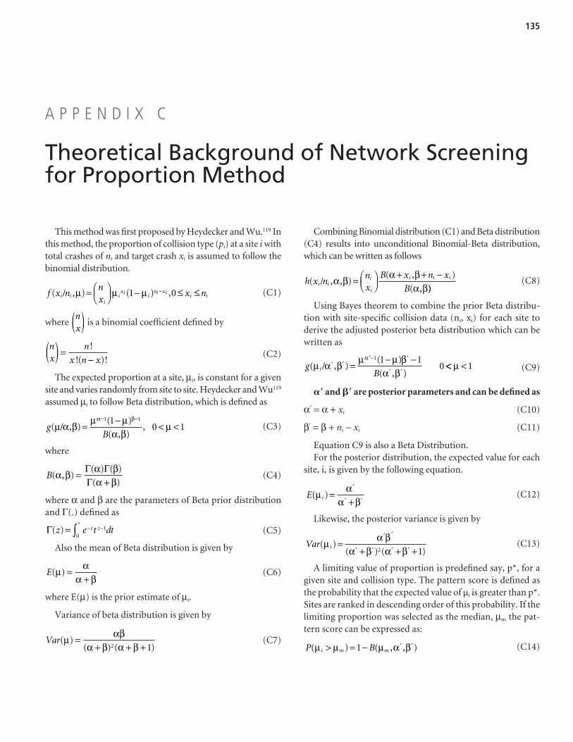
135

This method was first proposed by Heydecker and Wu.119 Inthis method, the proportion of collision type (pi) at a site i withtotal crashes of ni and target crash xi is assumed to follow thebinomial distribution.

(C1)

where is a binomial coefficient defined by

(C2)

The expected proportion at a site, μi, is constant for a givensite and varies randomly from site to site. Heydecker and Wu119

assumed μi to follow Beta distribution, which is defined as

(C3)

where

(C4)

where α and β are the parameters of Beta prior distributionand Γ(.) defined as

(C5)

Also the mean of Beta distribution is given by

(C6)

where E(μ) is the prior estimate of μi.

Variance of beta distribution is given by

(C7)Var( )( ) ( )

μ αβα β α β

=+ + +2 1

E( )μ αα β

=+

Γ( )z e t dtt z= − −∫ 10

°

B( , )( ) ( )

( )α β α β

α β=

+Γ ΓΓ

gB

( / , )( )

( , ),μ α β μ μ

α βμ

α β= − < <

− −1 110 1

nx

n

x n x( ) =−!

!( )!

nx( )

f x nnx

x ni ii

ixi

ini xi

i i( / , ) ( ) ,μ μ μ= ⎛⎝⎜

⎞⎠⎟ − ≤ ≤−1 0

Combining Binomial distribution (C1) and Beta distribution(C4) results into unconditional Binomial-Beta distribution,which can be written as follows

(C8)

Using Bayes theorem to combine the prior Beta distribu-tion with site-specific collision data (ni, xi) for each site toderive the adjusted posterior beta distribution which can bewritten as

(C9)

�� and �� are posterior parameters and can be defined as

α′ = α + xi (C10)

β′ = β + ni − xi (C11)

Equation C9 is also a Beta Distribution.For the posterior distribution, the expected value for each

site, i, is given by the following equation.

(C12)

Likewise, the posterior variance is given by

(C13)

A limiting value of proportion is predefined say, p*, for agiven site and collision type. The pattern score is defined asthe probability that the expected value of μi is greater than p*.Sites are ranked in descending order of this probability. If thelimiting proportion was selected as the median, μm the pat-tern score can be expressed as:

(C14)P Bi m m( ) ( , , )μ μ μ α β> = −1 ′ ′

Var i( )( ) ( )

μ α βα β α β

=+ + +

′ ′

′ ′ ′ ′2 1

E i( )μ αα β

=+

′

′ ′

gB

i( / , )( )

( , )μ α β μ μ β

α β

α′ ′

′ ′

′ ′= − −−1 1 1

0 << <μ 1

h x nnx

B x n x

Bi i

i

i

i i i( / , , )( , )

( ,α β α β

α β= ⎛

⎝⎜⎞⎠⎟

+ + −))

A P P E N D I X C

Theoretical Background of Network Screeningfor Proportion Method

Parameter Estimation of Beta Prior Distribution

The parameters α and β of the Beta distribution can beexpressed in terms of moments (mean and variance) asshown in equations C15 and C16. The mean and variancefrom the observed data are used to estimate α and β.

To illustrate, suppose there are 1, 2, 3, . . .i, . . .m sites underconsideration. μi is the proportion of a specific collision type forsite i, that is μi = xij / ni, where xij is the total number of target col-lisions of type, j, during the study period at site i and ni is thetotal number of all types of collisions at site i during the sameperiod. The mean proportion of target collisions, j, is given by

(C15)

where is the mean proportion of target collision type j.

Similarly, the variance is given by

(C16)

For a sufficiently large sample, the sample mean, , rep-resents the expected value, E(μj) and the sample variance, s2,represents the population variance, Var(μ). The variance canalso be expressed as

(C17)

This can be further simplified as

(C18)

This gives

(C19)α μ μ μ= − −2 3 2

2

s

s

s22

11

11

=−

⎛⎝⎜

⎞⎠⎟

+⎛⎝⎜

⎞⎠⎟

μ

μαμ

s2

22

2

1

=−

⎛⎝⎜

⎞⎠⎟

+⎛⎝⎜

⎞⎠⎟

αμ

α

αμ

αμ

μ j

sm

x x

n n m

x

ni i

i i

i

ii

m

i

22

21

21

1

1=−

−−

⎛⎝

⎞⎠ − ⎛

⎝⎜⎞⎠⎟=

∑==∑⎡

⎣⎢

⎤

⎦⎥ ≥

1

2m

n,

μ j

μμ

j

ij

i

m

m= =

∑1

Then β can be estimated as

(C20)

Posterior Beta Distribution and Pattern Score

The median, μm, of beta prior distribution is such that

(C21)

Once α and β are estimated, μm can be estimated using anMicrosoft Excel worksheet function.

The posterior parameters, α′ and β′, can be calculated byusing equations C10 and C11. The pattern score can be cal-culated using equation C14.

To summarize the above discussion, following is a stepwiseprocedure to estimate the parameters of beta prior and betaposterior distributions, and thereby the pattern score.

1. Divide the sites into logical groups. For example, two-lane rural roads analyzed separately from multilaneroads.

2. Identify the different types of collisions.3. Find total number of collisions of each type during the

study period in each site, xi.4. Find total number of all types of collisions in each site, ni.5. Calculate the proportion, xi/ni for each site and for each

type of collision of interest.6. Calculate the mean of the proportions for each collision

type, .7. Calculate variance using equation C16.8. Calculate α and β using equations C19 and C20.9. Estimate the median of Beta prior distribution using

Excel function (μm = betainv(0.5, α, β)).10. Calculate parameters of posterior Beta distribution as

α′ = α + xi and β′ = β + ni – xi.11. Estimate the pattern score using Excel function as P(μi >

μm) = 1-betadist (μm, α′, β′).

μ j

g dm

( ) / , ) .μ α β μη

=∫ 0 51

β αμ

α= −

136

137

Consider the data in Table 42, which pertains to crashcounts at 3,699 one-mile road segments in Utah. These seg-ments averaged 0.281 crashes per year during 1995 to 1997and 0.279 crashes per year during 1998 to 2000, further evi-dence that they were largely unaltered during the 6-yearperiod from 1995 to 2000, according to information in theHighway Safety Information System (HSIS)108 from whichthese data were extracted. In Table 42, segments are groupedinto rows based on the count of crashes during 1995 to 1997.As the last column shows, those segments in groups whichduring 1995 to 1997 had more than the average number ofcrashes in this period (0.281 crashes per year or 0.843 crashesin 3 years) experienced a reduction in crashes during 1998to 2000. Segments with fewer crashes than the average (i.e.,those with 0) experienced a considerable increase.

These changes are due to random fluctuations in short-term counts that result in a phenomenon known as regression

to the mean. The result is that such changes can be erro-neously attributed to a countermeasure in an observationalstudy that simply compares crashes before and after imple-mentation. In particular, if the segments with high counts areselected for treatment (as often happens) the positive effectsof the treatment in such a naïve study would be exaggeratedby the amounts shown in the last column of the earlier rowsin the table. This random fluctuation also suggests that a sitewith a higher collision count is not necessarily a stronger can-didate for safety improvement than a site with a lower count.The upshot of this phenomenon is that the crash count byitself is not good enough for estimating the safety of a site foruse in identifying candidate improvement locations and inestimating the safety effect of potential or implemented coun-termeasures. This is why more sophisticated predictive guidesare needed. Evidence of regression to the mean in two otherstates’ data used for this study is presented in Tables 43 and 44.

A P P E N D I X D

Illustrating Regression to the Mean

Crashes 3 yrs Prior

Number of Sites

Crashes 1995-1997

Crashes 1998-2000 % difference

17 17 416 340 -18.3 16 6 96 86 -10.4 15 8 120 97 -19.2 14 6 84 73 -13.1 13 5 65 45 -30.8 12 5 60 57 -5.0 11 11 121 101 -16.5 10 12 120 119 -0.8 9 17 153 112 -26.8 8 14 112 99 -11.6 7 19 133 108 -18.8 6 34 204 194 -4.9 5 34 170 160 -5.9 4 51 204 175 -14.2 3 93 279 250 -10.4 2 173 346 282 -18.5 1 431 431 377 -12.5 0 2763 0 431 infinite increase

Table 42. Wildlife–vehicle crash data for Utah illustrating regressionto the mean.

138

Crashes 3 yrs Prior

Number of Sites

Crashes 1996-1998

Crashes 1999-2001 % difference

32 6 242 227 -6.2 31 3 93 65 -30.1 30 3 90 70 -22.2 29 3 87 29 -66.7 28 1 28 23 -17.9 27 2 54 50 -7.4 26 1 26 19 -26.9 25 5 125 115 -8.0 24 5 120 91 -24.2 23 3 69 43 -37.7 22 1 22 20 -9.1 21 10 210 174 -17.1 20 3 60 37 -38.3 19 7 133 103 -22.6 18 8 144 105 -27.1 17 4 68 45 -33.8 16 7 112 89 -20.5 15 19 285 213 -25.3 14 28 392 303 -22.7 13 39 507 450 -11.2 12 33 396 338 -14.6 11 44 484 386 -20.2 10 55 550 404 -26.5 9 94 846 746 -11.8 8 114 912 654 -28.3 7 144 1008 779 -22.7 6 216 1296 1145 -11.7 5 290 1450 1179 -18.7 4 429 1716 1321 -23.0 3 653 1959 1728 -11.8 2 1167 2334 2066 -11.5 1 2518 2518 2482 -1.4 0 13125 0 2586 Infinite increase

Table 43. Data for North Carolina illustrating regression to the mean.

Crashes 3 yr s Prior

Number of Site s

Crashes 1997-1999

Crashes 2000- 2002 % difference

6 8 61 41 -32.8 5 8 40 27 -32.5 4 21 84 41 -51.2 3 55 165 84 -49.1 2 147 294 149 -49.3 1 792 792 343 -56.7 0 11941 0 951 infinite increase

Table 44. Data for California illustrating regression to the mean.

139

The literature description for this appendix contains stand-alone references. The literature review of all other appendicesis contained in the References section.

I. Wildlife-Vehicle Collision AnalysisAllen, R.E., and McCullough, D.R. 1976. Deer-car accidents in south-

ern Michigan. Journal of Wildlife Management 40(2):317–321.Bashore, T.L., Tzilkowski, W.M., and E.D. Bellis. 1985. Analysis of deer-

vehicle collision sites in Pennsylvania. Journal of Wildlife Manage-ment 49(3): 769–774.

Bellis, E.D., and H.B. Graves. 1971. Deer mortality on a Pennsylvaniainterstate highway. Journal of Wildlife Management 35(2):232–237.

Biggs, J., Sherwood, S., Michalak, S., Hansen, L., and C. Bare. 2004.Animal-related vehicle accidents at the Los Alamos National Lab-oratory, New Mexico. The Southwestern Naturalist 49(3):384–394.

Caryl, F.M. 2003. Ungulate mortality on a forested highway. Universityof East Anglia, Norwich. M.Sc. dissertation. 42 pp.

Finder, R.A., Roseberry, J.L., and A. Woolf. 1999. Site and landscapeconditions at white-tailed deer/vehicle collision locations in Illi-nois. Landscape and Urban Planning 44: 77–85.

Gundersen, H., and H.P. Andreassen. 1998. The risk of moose-collision:a logistic model for moose-train accidents. Wildlife Biology 4(2):103–110.

Gundersen, H., Andreassen, H.P., and T. Storaas. 1998. Spatial andtemporal correlates to Norwegian train-moose collisions. Alces 34:385–394.

Hubbard, M.W., Danielson, B.J., and R.A. Schmitz. 2000. Factors in-fluencing the location of deer-vehicle accidents in Iowa. Journal ofWildlife Management 64(3):707–713.

Joyce, T.L., and S.P. Mahoney. 2001. Spatial and temporal distributionsof moose-vehicle collisions in Newfoundland. Wildlife Society Bul-letin 29(1): 281–291.

Kassar, C., and J.A. Bissonette. 2005. Deer-vehicle crash hotspots inUtah: data for effective mitigation. UTCFWRU Project Report No.2005(1):1-28. Utah Cooperative Fish and Wildlife Research Unit,Utah State University, Logan Utah.

Malo, J.E., Suarez, F., and A. Diez. 2004. Can we mitigate wildlife–vehicle accidents using predictive models? Journal of Applied Ecol-ogy 41: 701–710.

Nielsen, C.K., Anderson, R.G., and M.D. Grund. 2003. Landscape in-fluences on deer-vehicle accident areas in an urban environment.Journal of Wildlife Management 67(1): 46–51.

Nielsen, S.E., Herrero, S., Boyce, M.S., Mace, R.D., Benn, B., Gibeau,M.L., and S. Jevons. 2004. Modelling the spatial distribution ofhuman-caused grizzly bear mortalities in the Central Rockiesecosystem of Canada. Biological Conservation 120:101–113

Premo, D.B.P., and E.I. Rogers. 2001. Town of Amherst deer-vehicle ac-cident management plan. White Water Associates, Inc., Amasa,Michigan (www.white-water-associates.com)

Rogers, E. 2004. An ecological landscape study of deer-vehicle collisionsin Kent County, Michigan. Report for the Michigan State Police,Office of Highway Safety and Planning. White Water Associates,Inc., Amasa, MI 49903. 56 pp.

Romin, L.A. and J.A. Bissonette. 1996. Temporal and spatial distributionof highway mortality of mule deer on newly constructed roads atJordanelle Reservoir, Utah. The Great Basin Naturalist 56(1): 1–11.

Seiler, A. 2005. Predicting locations of moose-vehicle collisions in Swe-den. Journal of Applied Ecology 42: 371–382.

Simek, S.L., Jonker, S.A., and Mark J. Endries. 2005. Evaluation of prin-cipal roadkill areas for Florida black bear. ICOET 2005.

Singleton, P.H., and J.F. Lehmkuhl. 1999. Assessing wildlife habitatconnectivity in the Interstate 90 Snoqualmie Pass Corridor, Wash-ington. ICOWET III.

II. Spatial Analysis TechniquesBoots., B.N. and A. Getis. 1988. Point Pattern Analysis. Sage Publica-

tions, Inc. Newbury Park, California. 85 pp. Burka, J., Nulph, D., and A. Mudd. 1997. Technical approach to devel-

oping a spatial crime analysis system with ArcView GIS. INDUSCorporation and U.S. Department of Justice.

Lee, J., and D.W.S. Wong. 2001. Statistical Analysis with ArcView GIS.John Wiley and Sons, Inc., New York, New York. 192 pp.

Levine, N., Kim, K.E., and L.H. Nitz. 1995. Spatial analysis of Honolulumotor vehicle crashes: I. Spatial Patterns. Accident Analysis and Pre-vention 27(5):663–674.

Levine, N. 1996. Spatial statistics and GIS: software guides to quantifyspatial patterns. Journal of the American Planning Association 62(3):381–391.

Levine, N. 1999. Quickguide to CrimeStat. Ned Levine and Associates,Annandale, VA.

Levine, N. 2004. CrimeStat III: Distance analysis. Chapter 5 in: A spa-tial statistics program for the analysis of crime incident locations. NedLevine & Associates: Houston, Texas, and the National Institute ofJustice, Washington, D.C., USA.

A P P E N D I X E

A Literature Review of Field Studies and Spatial Analyses for Hotspot Identificationof Wildlife–Vehicle Collisions

Spooner, P.G., Lunt, I.D., Okabe, A. and S. Shiode. 2004. Spatial analy-sis of roadside Acacia populations on a road network using the net-work K-function. Landscape Ecology 19:491–499.

I. Wildlife–Vehicle Collision AnalysisAllen, R.E., and D.R. McCullough. 1976. Deer-car accidents in south-

ern Michigan. Journal of Wildlife Management 40(2): 317–321.

Objective: to identify the time, place, and characteristics of traffic anddeer that contribute to collisions. It was hoped that such an under-standing would suggest measures to reduce collisions

Data layers: 10 counties in S. Michigan; data on DVC from accident re-ports, 1966-1967• Variables analyzed for all accidents: date, day of week, time,

speed of car, sex of deer, road type• Added to 1967 data: location within 0.16 km from a landmark;

number deer seen at time of accident; fate of deer involved;whether car driven or towed away; extent of injuries

• Traffic volume data from MI Dept of State Highways: averagetraffic volume for various time intervals (hourly, daily, monthly)

Analyses: 3 areas from highest accident roads chosen for habitat analy-sis: all accidents plotted on aerial photos and roadside habitat clas-sified as cropland, forest, or unimproved field

Results: most accidents occurred between 1600–0200; 2 peaks, sunriseand 1-2 hours after sunset; traffic volume and DVC correlated forevening and nighttime hours (85% of variation in DVC accountedfor by traffic volume)• Number of accidents and traffic volume highest on weekends;

largest number of DVC in fall and early winter• In 3 sections where habitat determined, accidents and habitat

types occurred in similar proportions• % of accidents increased up to a speed of 80-95 kph, then de-

clined at higher speeds

Bashore, T.L., Tzilkowski, W.M., and E.D. Bellis. 1985. Analysis ofdeer-vehicle collision sites in Pennsylvania. Journal of WildlifeManagement 49(3): 769–774.

Objectives: examined roadkill locations plotted on highway maps by PAGame Protectors since 1968. A cursory exam revealed that deer killstend to be aggregated at specific sites where accidents occur yearafter year. Analyzed aerial photos and highway and topo maps andconducted field studies to determine which factors characterizeconcentrations of collisions at particular sites. A model was devel-oped to predict probabilities that a section of highway would be ahigh kill site and then tested for reliability.

4 PA counties studied, used 2-lane hard-top roads, 51 paired sites (killand control), data collected from 1 July–30 Oct 1979 and 27 June–1 Oct 1980

Data layers: residences (number/ha); commercial buildings (num-ber/ha); other buildings (number/ha); banks (prop. of terrain ele-vated more than 1 m above road surface); gullies (more than 1 mbelow road surface); level (not bank or gully); wooded; non-wooded; barren; distance to woodland; increasing slope; decreas-ing slope; no slope; angular visibility; in-line visibility; shortest vis-ibility; speed limit; fencing; guardrails

Data obtained by selecting a random point from within each 100m in-terval of site length and running a 100 m transect perpendicularly

from each side of the road; at sites shorter than 100 m, two pointswere randomly selected

Analysis: stepwise logistic regression used to test the importance of thevariables used in the model; 5 pairs of sites randomly selected for atest of the model’s predictive ability

Results: 9 of 19 variables selected for inclusion in model (residences, com-mercial buildings, other buildings, shortest visibility, in-line visibil-ity, speed limit, distance to woodland, fencing, non-wooded area); • 85% of kill locations had a prob. of 0.70 or greater of being clas-

sified as kill site; 89% of control had a prob. of 0.30 or less ofbeing classified as kill site

• high correlation between speed limit and in-line visibility; be-tween residences and other buildings; removal of correlatedvariables did not significant change model

• 9 and 7 variable models performed equally well in predicting killand non-kill sites; 5 kill locations correctly classified, one con-trol location misclassified by both models

Discussion: DVCs not random in time or space; kills aggregated

Bellis, E.D., and H.B. Graves. 1971. Deer mortality on a Pennsylvania in-terstate highway. Journal of Wildlife Management 35(2): 232–237.

Objective: to present the results of an analysis of data on highway mor-tality collected from November 1968 through December 1969

Data layers: data collected from an 8.03-mile section of I-80; dividedinto 212 contiguous sectors of 200 ft length• Kill data obtained from game protector who filled out re-

searcher-supplied data sheets (date, location by sector number,highway lane, sex, age class); it was understood that many killswere probably not reported

• 5 portions of each of the 212 sectors analyzed for physical andvegetation factors that might affect deer mortality: plantedROW on each side of highway; area adjacent to ROW on eachside of highway; median strip

• Factors used in the analyses: quality and amount of vegetation;topography; area of ROW; presence of fences or guardrails

• Deer counts obtained from May 68–May 69 by spotlightingfrom vehicle

Results: 286 reported DVC; 67.9% of sectors had at least one DVC (maxof 9 in one sector); roadkills often concentrated in groups of con-tiguous sectors• 70% of deer seen through spotlighting were grazing (conserva-

tive estimate); suggests presence and type of vegetation withinsectors accounted for much of variation in numbers killed

• Low correlation between DVC and all measured variables—demonstrated that with our technique we could not account forthe variation in numbers of deer killed

• Examined data in a less analytical manner by considering com-bos of sectors in relation to overall topography– High mortality: (1) where sections of road lay in troughs

formed by elevated median strips with steep banks and steepinclines on ROW; (2) where troughs terminated by reduc-tions in elevation of the median strips allowing deer to easilycross road; (3) both sides of highway and median strip hadgood grazing and relief relatively flat

– Low mortality: (1) area with low relief, abundant food onROW and chain link fence; (2) ROW declines sharply to astream or other lowland area, guardrails present

• High correlation between number killed per month and num-ber seen per month

140

Biggs, J., Sherwood, S., Michalak, S., Hansen, L., and C. Bare. 2004.Animal-related vehicle accidents at the Los Alamos National Labo-ratory, New Mexico. The Southwestern Naturalist 49(3): 384–394.

Objectives: to (1) analyze wildlife–vehicle accident data with respect totime, season, location, and species for accidents occurring onLANL internal and perimeter roads and (2) perform an analysis ofsite characteristics at accident locations identified as hotspots.

Data layers: ~68 km of primary rd included in study; majority of trafficvolume in early morning and late afternoon; WVC data from1990–1999• Accident data: from NMDGF, LAPD and LANL security force

reports (date, time, location, species, cost of damage, injuries tohumans, injuries to animals); accident locations recorded intoGIS (sometimes based on approximate description of site)

• Hotspot characterization data: vegetation characteristics (dom-inant tree, shrub, forbs and grass sp.), posted speed limit, roadtype (straight, curve, hill), presence of lighting, amount of avail-able light (high, mod, low, none), presence and length ofguardrails, height of fencing, slope characteristics, motorist vis-ibility distance

Analyses: Cluster analysis using GIS nearest neighbor index approachused to determine whether accidents were distributed randomly;deer and elk examined separately• Density analysis using the “simple” type calculation of the GIS

program and a search radius of 100 m applied to identify acci-dent hotspots

• Accident site characterization analysis: 15 hotspots selected,with 15 paired control sites; 100 m transect centered on siteplaced parallel to road on either side, six 15 m transects (at 25,50, 75 m marks) placed perpendicular to 100 m transects;hotspot characterization data recorded along 15 m transects

• Statistical analyses: χ2 used to test for differences in accidentcounts between seasons– Exact binomial tests: to determine if differences occurred be-

tween the numbers of accidents in different pairs of seasons;also if significant difference occurred among hourly countsof accidents; deer and elk analyzed separately

– Poisson regression: if accident count in given year significantdifference from other years; also to test if association betweenmonthly accident counts and monthly snowfall amounts sig-nificant; deer and elk analyzed separately

– Logistic regression: to model status of an area as a hotspot orcontrol as a function of measured variables

– Fisher’s exact test: if diff in recoded variables betweenhotspots and controls were statistically significant

– Univariate logistic regression: as first step to identify poten-tial predictors for a larger model; potential predictor vari-ables chosen if (1) absolute value of the Wald statistic > 1, (2)lit search revealed potential importance, or (3) authorsthought important

Results: seasonal peaks in DVC (fall) and E(lk)VC (winter, fall); mostaccidents in late afternoon and evening hours• Cluster analysis: EVC and DVC did not occur randomly• Density analysis: identified several areas with higher concentra-

tions of accidents• Accident site characteristics: when considered 1 at a time, no

variable measured was a statistically significant predictor ofhotspot or control status; variables chosen as predictors in finalmodel were ln(average number woody stems > 2 m in height),and maximum slope

Discussion: ambiguous relationship between accidents and snowfallmight derive from our pooling of snowfall and accident data bymonth instead of using daily snowfall measurements and accidentcounts• Poor results with utility of different variables could be result of

small sample size• Because of small sample size, placed a higher priority on finding

a well-fitting model that made sense rather than on finding onethat was statistically significant

Caryl, F.M. 2003. Ungulate mortality on a forested highway. Universityof East Anglia, Norwich. M.Sc. Dissertation (copyrighted) 42 pp.

Objective: to produce a multi-species empirical model of ungulate roadmortality using highly accurate spatial data from field and GISbased sources in Kootenay National Park, British Columbia,Canada. It would then be determined if the model could be repro-duced using GIS-based variables only, to provide a quick and ef-fective management guide to focus mitigation efforts at high risklocations

Data layers: species included moose, mule deer, white-tailed deer, elkand bighorn sheep• Ungulate mortality data: date, number, species, sex, age, loca-

tion from GPS • Control site data: randomly selected non-kill sites along high-

way; ratio of control sites to kill sites larger than one desirabledue to greater expected variation in control environmental attributes

• Field-based environmental variables: distance to cover (> 1 mtall and continuous), % cover forest; % cover shrub; % coverherb; % cover bare ground; roadside slope; verge slope; adjacentland slope; inline visibility; angular visibility

• GIS-based variables (using ArcView): elevation; distance to hy-drology; distance to human use; road sinuosity ratio; change inelevation; habitat importance for deer, moose and elk; barrier

Analysis: Spearman’s rho correlations used to screen for multi-collinearity, removed one highly correlated biophysical variable be-fore model development; differences between seasons comparedusing χ2 tests• Model development: logistic regression, stepwise selection

process using log likelihood ratio tests and a prob. value of 0.05for entry and removal of variables to the model; selectionprocess then repeated using only GIS-based variables; χ2 used asa goodness-of-fit test of model appropriateness; Wald stats totest the significance of independent variables; direction of pre-dictor influence verified using Mann-Whitney U tests; odds ra-tios examined to assess contribution that a unit increase in pre-dictor variable made to outcome probability

• Model validation: 5 control and 5 kill sites randomly chosen tovalidate model’s predictive ability; 0.29 chosen as classificationcut-off for predicted group memberships based number of kill sites vs control sites; predicted probabilities classified into3 groups: low, moderate and high risk of kill

Results: Kill sites highly aggregated; highly significant seasonal differ-ences (high in summer); roadkills positively associated with dailytraffic volumes• 3 of 17 environmental variables shown to be reliable predictors:

distance to humans, elevation, distance to cover; all had nega-tive coefficients; 67.3% kill sites, 64.3% control sites predictedcorrectly, giving overall success of 65.2%

141

• 2 of 9 GIS variables shown to be reliable predictors: distance tohumans, elevation; both had negative coefficients; 61.5% killsites, 65.1% control sites predicted correctly, giving overallsuccess of 64%

• Model testing: 3 of 5 control sites, 4 of 5 kill sites (70% of sites)correctly classified using GIS model

• Probability surface with low moderate and high collision prob-ability created using 2 GIS variables

Discussion: kill sites not located randomly in time or space; kill sitesfound at lower elevations than control sites and closer to humanuse areas; odds of a kill decreased by 96% with each additional 1000m elevation above sea level if all other variables controlled; odds ofa kill decreased by 40% with each additional 1 km distance fromhuman disturbance sites; probability surface showed a close agree-ment with observed roadkill locations, would be useful guide forquick assessment of possible high risk locations

Finder, R.A., Roseberry, J.L., and A. Woolf. 1999. Site and landscapeconditions at white-tailed deer/vehicle collision locations in Illi-nois. Landscape and Urban Planning 44: 77–85.

Objective: to determine if high deer/vehicle accident locations could bepredicted from remotely sensed land use/land cover patterns

Data layers: 98 counties in IL; 1989–1993; rd segments with high con-centrations of DVAs on state marked routes; n=86 locations with ≥15 reported DVAs analyzed• Plotted hotspot road segments using TIGER data files and Map

and Image Processing System GIS software; road segments ad-justed to 1.3 km; random locations on same route of samelength for control purposes

• Landcover classification (Landsat TM): crops, forest, grass,water, developed, orchards; topographic physical features fromaerial photographs and topographic maps

Analyses: 0.8 km radius buffer zone around each road segment to quan-tify and compare landscape composition and pattern usingFRAGSTATS• Simple correlation used to investigate relations among variables;

highly correlated eliminated• t-tests to determine if variable means differed between hotspots

and controls; those indices with |t| values ≥ 3.0 selected as pre-dictor variables for logistic regression

• Stepwise logistic regression model selection process to obtain apreliminary equation

• AIC to compare models• Stepwise selection process repeated using only landscape in-

dices, satellite imagery data only• 5 paired sites used to test models’ predictive abilities

Results: variables included in model 1: % distant woody cover, % adja-cent gully; natural log of area of recreational land within buffer,natural log of width of corridors crossing road; of 10 samples to testmodel validity, 5 control and 4 hotspots correctly predicted• Variables included in model 2: Simpson’s diversity index; natu-

ral log of woods mean proximity index; of 10 samples to testmodel validity, 4 control and 2 hotspots correctly predicted

Discussion: study demonstrated that DVA site statistics and RS habitatand highway data can be used to predict DVA locations

Gundersen, H., and H.P. Andreassen. 1998. The risk of moose-collision: a logistic model for moose-train accidents. Wildlife Bi-ology 4(2): 103–110.

Objective: to use a logistic model to establish the most risky train de-partures for Rørosbanen railway which has the highest risk of

moose-train collisions per km in Norway (Gundersen et al. 1998).In the model we have included speed of train, type of train, time ofday and lunar phase, besides climatic covariables known to be cor-related with moose-train collisions.

Data layers: success (1) or failure (0) of train hitting moose; train departures; train route; train predictor variables (average

speed, train type, time of day); daily average temperature; snow depth; lunar phase; data recorded from Dec-Mar 1990-1997

Analysis: a logistic model was applied incorporating the above variables; the most parsimonious model chosen using AIC;another model made containing only passenger trains running the

whole distance between 2 towns, snow depth, daily averagetemp, lunar phase, train speed, time of day left station;

used data from 1990–1996 to predict the number of train-killedmoose for each train for the winter of 1996/1997

Results: most parsimonious model included route, time of day, lunarphase, snow depth, temp; according to AIC, this model is indistinguishable from one includ-

ing average train speed;best model for the second analysis included all predictor variables.Problems with morning train results in second analysis due to in-

troduction of logging activity in Storholmen in 1996.Second model gave good results for morning train after removing

6 collisions at Storholmen

Discussion: authors introduced a new approach to study game-vehicleaccidents by focusing on factors that cause vehicles to collide withgame rather than focusing on the factors that cause game to be closeto traffic arteries.

Gundersen, H., Andreassen, H.P., and T. Storaas. 1998. Spatial andtemporal correlates to Norwegian train-moose collisions. Alces34: 385–394.

Objectives: In this study we reveal how temporal variation, i.e. climaticfactors and moose population density, and spatial variation, i.e.landscape pattern and changes in food availability, correlate withmoose–train collisions along the railway in Norway which is mostburdened by wildlife collisions.

Data layers: train kills (time, location to nearest 100 m)daily average temperature, snow depthsize of moose pop estimate by population model Cersim (based on

observations by hunters in previous season)

Analysis: 2 categories of analysis—temporal factors (climatic and pop den-sity) and spatial factors (landscape patterns and food availability)• Temporal factors: compared the freq. distribution of days w/

certain weather conditions (expected) w/ the freq. distributionof collisions at the various weather conditions (observed) by agoodness-of-fit test. GLMs used to correlate moose pop size andnumber of collisions

• Spatial factors (regional): analyzed correlation between land-scape patterns and number of collisions per 1 km segment – Landscape patterns: (1) topography—measured as the dif-

ference in height from the bottom of the valley to the highestpoint within 2.5 km to East and West of line and averaged;(2) distance to the nearest side valley—because assumed tochannel moose migratory behavior;

– Tested and corrected for autocorrelation in 1 km segments• Spatial factors (local): to explain spatial variation of collisions,

compared number of collisions before and after changes in foodavailability due to logging activity in two areas

142

– One area had increased food availability while the second haddecreased food availability

– Linear model including factors that significantly correlated toyearly variation in collisions (climatic factors and populationdensity) used to obtain estimate of expected number of col-lisions before and after change in food availability; expectedvs observed compared with goodness-of-fit test

Results: Temporal effects: number of collisions associated with bothtemp and snow depth; combined temp and snow depth into vari-able (accidental period) which started when snow depth exceeded30 cm and lasted until temp stabilized above 0 degrees C. Numberof days in new variable explained 83% of yearly variation in num-ber of moose collisions; GLM including both accidental period andpop density explained 88% of yearly variation

Spatial effects: significant negatively correlated between number of col-lisions and distance to nearest side valley; no association betweennumber of collisions and topography; changes in food availabilitystrongly associated to number of collisions

Discussion: moose usually killed in winter on days with lots of snow andlow temps; influenced by migratory routes to lower elevations andavailability of food; temporal variation due to climatic factors, spa-tial variation due to migratory routes and food availability.

Hubbard, M.W., Danielson, B.J., and R.A. Schmitz. 2000. Factors in-fluencing the location of deer-vehicle accidents in Iowa. Journalof Wildlife Management 64(3):707–713.

Objective: to examine the influence of highway and landscape variableson the number of DVAs in Iowa

Data layers: number of DVAs, traffic and landcover data obtained forall milepost markers within the state (n = 9,575)• GIS maps of habitat (Landsat imagery, 1990–1992): collapsed

habitat types into cropland, woody cover, grass, artificial, waterand miscellaneous

• White-tailed deer harvest numbers for each county from IDNR;DVAs from 1990–97 for state’s highways from IDOT; traffic vol-ume estimates linked to all accident sites

• For each DVA included: distance to nearest town or city, dis-tance to nearest city with pop > 2,000, number of bridges, num-ber of lanes of traffic

• Accident location often recorded to nearest 0.10 mile, but morethan 33% recorded at milepost, therefore all locations collapsedto nearest milepost

Analysis: dependent variable-number of accidents in each 1.61 km seg-ment from 1990–97• Randomly selected sample sites (n = 1,284); clipped 2.59 km2

landscape section with sample site• FRAGSTATS used to characterize landscape sections; linked to

number of DVAs for segments• DVAs separated into 2 categories (0-13, > 14 hits/segment)

based on natural break and sample size• Logistic regression: to examine relationship of DVAs to traffic,

highway characteristics, human pop centers, and landscape vari-ables; stepwise selection procedure for variable inclusion duringmodel development

• Factor classification tree (FCT) constructed to refine ability toselect high DVC areas– Robust relative to a more standard cluster and discrimination

analysis that might be used (Emmons et al. 1999)– Followed method described by Venables and Ripley (1994)

to find the rooted subtree with a minimum AIC

• Evaluated performance of logistic regression model by applyingto a randomly selected set of DVA sites not included in modeldevelopment (n = 245)

Results: 67% of 9,575 mileposts associated with DVA; > 25% DVAs at3.4% of mileposts (325)• Significant 6-variable model produced; 4 variables landscape

features, 2 highway characteristics• FCT final classification produced a tree with 57 nodes and a mis-

classification rate of 0.153%; bridge frequency was best predic-tor of high DVA sites

• Model validation: correctly classified 63.3% of sites

Discussion: edges not found to be important, however it is possible thatthe resolution of our data was too coarse to identify all edges usedby deer as travel corridors. Bridges always indicate points wheremajor edge-creating landscape features intersect roadways, andtherefore may be better predictors of concentrations of DVAs thanmore broadly defined edge indices

Joyce, T.L., and S.P. Mahoney. 2001. Spatial and temporal distribu-tions of moose-vehicle collisions in Newfoundland. WildlifeSociety Bulletin 29(1): 281–291.

• Objective: “we . . . relate rate & severity of human injury to timeof accident, road conditions, road alignment, vehicle speed (viaposted speed limits), number of vehicle occupants, and sex/ageof moose struck . . . to develop measures to reduce MVCs andseverity of injuries”

• MVC reports from conservation officers and RCMP from1988–1994; accidents generally reported if damage > $1000 CD($500 CD before 1991).

• Spatial analyses: N = 1690 MVCs on Trans-Canada Highway,mapped/digitized, divided 900 km of TCH into ninety 10 kmsections. Category each section by – Annual average MVCs (< 1.75 = low, 1.75-3 = medium, and

> 3 MVCs = high)– Moose density (< 1.0 = low, 1-2 = medium, and > 2 = high)– Traffic volume (low vs. high)– Results:

� Areas of low or high moose densities experienced greaterprobabilities of MVCs than areas of moderate moosedensities.

� Higher probability of MVCs in areas with high trafficvolumes, regardless of moose densities

• MVCs and human injuries analyses: log linear modeling to eval-uate effects of the following variables on severity of humaninjuries (low vs. fatalities)– Darkness (day vs. dusk/dawn/dark)– Road condition (wet-slick vs. dry)– Road alignment (straight or curved)– Vehicle occupants (driver only vs. driver + passengers)– Posted speed limits (< 80 km/h vs. > 80 km/h)– Passenger vehicles only (made up 89.5 of all reported colli-

sions and had most serious injuries/fatalities)– Determined influence of each variable on injury severity

through forward model selection from main effects to sat-urated model; used log-likelihood value (G-sq) of main ef-fects model (included all variables) as baseline againstwhich all other parameters were judged; each 2-way inter-action was then added to main effects model and tested. De-viance between baseline value and derived G2 stat measuredimportance of that parameter to model. Excluded parame-

143

ters with small deviation, determined at 95% confidencelevel.

– Results: � No significant relationship between road alignment and ac-

cident severity (though 79% of accidents occurred on straightvs. curved roads)

� Model 1 (injury, darkness, speed): Light condition andposted speed limit related to severity, and mutually inde-pendent—risk 2.1x greater at night and 2x higher at high-way (high) vs. non-highway (low) speeds.

� Model 2 (injury, road condition, occupants): more acci-dents occur than expected when passengers were in vehi-cles on dry roads, but not when there were no passengersor wet roads. Risk of severe injury or death 2x higher w/atleast 1 passenger present compared to driver only.

• Also looked at temporal and age/sex influence . . .– Moose calves more likely to be involved Aug–Oct, yearlings

in June/July, and adults in July–Aug. – More bull moose involved than exp.– No significant relationship between diurnal patterns and sex

or age.– Injury 6x more likely in collision w/ adult than calf

• Discussion points of interest beyond results:– “Bashore et al. 1985 found positive relationship b/w speed

limit, driver in-line site visibility along road, and number ofcollisions (see also Poll 1989).”

– “Damas & Smith 1982 estimate night speeds have to be re-duced to 60km/hr or less under low-beam light to sufficientlyexpand stopping distances and prevent accidents...enforce-ment key and difficult/enormous . . . most effective measuremay be with drivers”

– Lavsund and Sandegren 1991. Moose vehicle collisions inSweden, a review. Alces 27:118–126. � “Lavsund and Sandegren (1991) found 3x increase in

severity of injury for vehicles moving 70–90km/hr com-pared to lesser rates”

– Discussed PR programs, mentioned Terra Nova NationalPark in Canada—long running program (12 yrs as of 2001)involving using moose silhouettes and posting of number ofMVCs/year; have found Newfoundland drivers perceiveTerra Nova National Park as area with greatest number andrisk of MVCs. See Hardy R.A. 1984. Resource managementplan for MVCs, internal Terra Nova NP Parks Canada report.

Kassar, C., and J.A. Bissonette. 2005. Deer-vehicle crash hotspots inUtah: data for effective mitigation. UTCFWRU Project ReportNo. 2005(1):1–28. Utah Cooperative Fish and Wildlife ResearchUnit, Utah State University, Logan Utah.

The data originate from collision reports prepared by law enforcementofficers and provided to UDOT by the Utah Department of PublicSafety. A wildlife–vehicle collision is included in the database onlyif an animal was actually hit, if the estimated vehicle damage ex-ceeded $1,000 and/or if a person was injured. Collisions includedin the database do not account for crashes that occurred as a resultof swerving to miss an animal.

We focus on collisions involving almost exclusively mule deer. We usedthe UDOT vehicle crash database to study DVC patterns and trendsfrom 1992–2002 on 248 state routes. We evaluated all routes forfrequency of deer kills and identified hotspots (at least 1 collision/mile/year). We considered hotspots to consist of two parts: (1) a

core area, the road segment where collisions per mile are most con-centrated; and (2) a mitigation zone, buffering segments on eachside of the core where appropriate mitigation actions can accountfor animal movement and behavior and help avoid the “end of thefence” problem.

Summary of results: 24,299 WVC over 11 years; 99.6% had dates andyears associated with them; average of 2,202 (2,025–2,577) colli-sions per year; 12 routes had high DVC rate over entire length (≥ 10/mile); 16 with moderate (5–9.99/mile); 148 with low rates(> 0–4.99); 65 routes with no reported DVC; 7 with data unavailable;54.6% of all collisions occurred on 10 routes

Collision frequency: 0–21.27 per mile; 1/3 occurred Oct–Dec; 55.7%occurred 1800–2400 hr

Hotspots: found 183 hotspots in Utah; core hotspots average 5.3 milesin length; isolated hotspots were 1 mile (1.6 km) in length; hotspotcollisions were concentrated; 57.74% of all collisions occurredwithin a cumulative (~ 1001 km) range, or 10.5% of total analyzedhighway miles (9,500 total km)

Malo, J.E., Suarez, F., and A. Diez. 2004. Can we mitigate wildlife–vehicle accidents using predictive models? Journal of AppliedEcology 41: 701–710.

Objective: the present study analyzed a European case and developedmodels of the environmental variables associated with the occur-rence of collisions with animals at two spatial scales (1.0 and 0.1km). Provided that a few variables underlie the location of animalcrossings, it should be possible to predict where accidents mayoccur and use this information to optimize mitigation efforts. Withthis aim, we (1) defined road sections with high collision rates usinga clustering detection procedure; (2) analyzed the landscape vari-ables of sections with high collision rates in contrast to low colli-sion sections; and (3) used a 0.1 km scale to analyze the pointswhere collisions occur in contrast to those where they do not.

Data layers: official traffic database on WVC for Jan 88–Feb 01; n =2,067; includes date, location (0.1 km); 63% of WVCs occurred be-tween 1998–2001; 98% involved roe deer, wild boar or red deer• Definition of high accident rd sections: determined by detecting

clusters of WVC locations; contiguity analysis conducted bycomparing the spatial pattern of collisions with that expected ina random situation; each km of rd with 3 or more collisions, es-pecially over consecutive km, could be defined as a high colli-sion section

• 1:50,000 digital forest cover map (cover types used: riparian for-est, other forest, scrub, grassland, crops, rivers and dams, ur-banized and unproductive); processed in ArcView 3.2

• Habitat features in high collision sections: analyzed 84 loca-tions—41 high collision, 43 low collision; sampling unit = cir-cular area (radius 1000 m) around reference point; calculatedproportion of each habitat type; ecotone length (meters ofcontact lines between habitat polygons); habitat diversity(Shannon index)

• Variables associated with collision point: analyzed at 0.1 kmscale: sampling points from 18 high collision sections in whichWVCs had been recorded in at least 12 hectometer posts; 6 hec-tometer posts with highest number WVCs chosen from eachsection; a further 6 taken at random from amongst those withrecorded collisions; 12 control samples w/o WVCs taken atrandom from each section

• Evaluated 13 quantitative and 15 qualitative variables coveringaspects linked to driving, general features of the road environs,features associated with animal movements; measurements

144

taken for 100 m rd stretch and evaluated 100 m on each side ofroad

Analysis: analyzed at both regional and local scales; predictive models forthe location of sections/points with and without collisions were gen-erated by binary logistic regression; validated with independent data• 2 models fitted for each analysis: 1 complete with all measured

variables, 1 reduced version with only most significant explana-tory variables

• Variable selection for reduced models using G2 statistic; ensurednew model was not significantly more informative than previ-ous one, avoided correlated variables and those w/o predictivecapacity

• Significant threshold in variable comparison: P = 0.05; proba-bility threshold for model: P = 0.1

Results landscape scale: 41 high collision rd section identified; 7.7% ofrd network accounting for 70.5% of all records; distributed amongsecondary and tertiary roads; none along A-2 fenced motorway• High collision areas had higher cover of non-riparian forest,

lower crop cover, lower urbanized areas, and higher habitat di-versity than low collision areas

• Simplified model included forest cover, urbanized area andhabitat diversity; had same predictive capacity as full model:87.0% correct classification for all cases, 88.5% for high and85.7% for low collisions sections; successfully predicted 70% of30 cases used as test data

Results for local scale: low collision areas associated with crossroads,underpasses, guard rails, embankments at least 2 m high with mod-erate or steep slopes, greater distances from roads to hedgerows andforest stands, and shorter distances from roads to buildings• Reduced model included presence of crossroads, presence and

continuity of guardrails, presence and continuity of embank-ments and distance to nearest forest stand; correctly predicted61.2% of cases, 72.7% of collision points, 48.4% of non-collisionpoints; full model results were 74.0%, 79.2% and 68.1% respec-tively; correctly classified 64.2% of test cases

Discussion: results show it is possible to predict the location of WVCsat 2 scales; results should be considered cautiously; validity couldbe hindered by assumption of a binomial distribution of errors—bigger issue for local rather than landscape model

Nielsen, C.K., Anderson, R.G., and M.D. Grund. 2003. Landscape in-fluences on deer-vehicle accident areas in an urban environment.Journal of Wildlife Management 67(1): 46–51.

Objective: quantified the effect of landscape factors on DVA in 2 Min-neapolis suburbs to provide public officials and wildlife managerswith recommendations for managing the landscape to reduceDVA.

Data layers: digitized DVA locations from 1993–2000 using ArcView• DVA clustering to differentiate DVA areas (≥ 2 DVA) and

control areas (0 or 1 DVA); overlaid 0.5 km road segments atmidpoint of DVA clusters; buffered road segments for variableselection purpose with a 0.1 km perpendicular distance fromedge of each side of road; repeated for control areas (n = 160total)

• Landscape variables: land cover (grassland/residential, wood-land, open water); land use (commercial/industrial, residential,public land); ArcView Patch Analyst used to calculate 60 classand landscape level variables; road curvature (straight orcurved); number of buildings in buffer, speed limit; number of

lanes; distance from road to nearest forest cover patch; ROWtopography based on presence or absence of ditches

Analysis: univariate procedure used to reduce 66 variable set to smallergroup; removed variables correlated at r ≥ 0.70; left with numberof buildings, number of forest cover patches, proportion of forestcover, Shannon’s diversity index for further analysis• Logistic regression analysis to determine which variables best

explained difference between DVA areas and control areas; builtone global model and 10 a priori models; used AIC and Akaike’sweights to rank and select best model; used relative weight ofevidence to compare parameter importance; model averaging toincorporate model-selection uncertainty into final uncondi-tional parameter estimates and standard errors

• 40 sites retained to validate best-fit model

Results: global model was significant; areas with DVA contained fewerbuildings, more patches and higher proportion of forest cover,more public land patches and higher Shannon’s diversity index oflandscape; Akaike’s weights indicated number of buildings andnumber of public land patches most important variables• 7 models necessary to compile a 95% confidence set; best-fit

model correctly classified 77.5% of test sites

Discussion: study unique because assessed landscape factors influenc-ing DVA in an urban environment; pooled data over 7-year periodso pop growth or land-use change may have affected data

Nielsen, S.E., Herrero, S., Boyce, M.S., Mace, R.D., Benn, B., Gibeau,M.L., and S. Jevons. 2004. Modelling the spatial distribution ofhuman-caused grizzly bear mortalities in the Central Rockiesecosystem of Canada. Biological Conservation 120:101–113

Objective: “We develop predictive models and maps that describe thedistribution of human-caused grizzly bear mortalities . . . Our goalwas to understand, through modeling, the relationships among bearmortality locations and landscape-level physiographic and humanvariables. More specifically interested in (1) examining the spatialdensity of grizzly bear mortalities; (2) evaluating possible differencesin the physiographic attributes of mortality locations . . .; and(3) developing predictive models that estimate the relative proba-bilities of bear mortality (risk) given multivariable combinations ofphysiographic variables.”

Data layers: mortality info from 1971–2002; included dead bears andtranslocated bears; location (UTM when possible), accuracy oflocation (accurate, reasonable, unknown), month, year, sex, age,and cause of mortality; n = 279 accurate and reasonable locations• GIS (spatial) predictor variables: land cover (Landsat TM 95-98,

5 classes); distance to edge of nearest land cover; greennessindex; distance to nearest water feature; distance to nearest lin-ear human use feature; terrain ruggedness index

Analyses: 3 separately scaled moving windows to calculate total densityof mortality locations: 520 km2; 900 km2; 1405 km2; secure sites =pixels with 0 mortalities; high mortality zones = pixels with > 31mortalities (≥ 1 mortality/year)• Logistic regression to assess relationship between landscape at-

tributes of mortality locations and categories of demographicstatus, season, and mortality type

• Random sample of locations generated to contrast with human-caused mortality locations

• Data divided into model training (80%) and model testing(20%) data sets

• Logistic regression used to contrast the location of grizzly bearmortalities with sites used by bears (through telemetry)

145

Results: mortalities concentrated within 3 regions regardless of scaleexamined• 900 and 1405 km2 scales: mortality densities within moving win-

dows exceeded 31 mortalities for the three sites; at 520 km2 scale:only one site as high mortality zone

• Total area occupied in high mortality zones: 520 km2 =1.4%, 900km2 = 3.8%, 1405 km2 = 13.2%

• Total area occupied in secure zone: 520 km2 = 23.9%, 900 km2 =13.9%, 1405 km2 = 23.9%; 22–32% secure habitat in areas ofnon-habitat

• Mortality locations positively associated with access, water, andedge features; negatively associated with terrain ruggedness andgreenness indices

• Non-harvest mortalities more likely to occur in shrub and grass-land habitats and closer to edge features and access than randompoints

• Mortalities more likely to occur in deciduous forest and shrubhabitats, nearer to edge, access, and water than radiotelemetrylocations; also sig related to areas of low greenness and minimalterrain ruggedness

Premo, D.B.P., and E.I. Rogers. 2001. Town of Amherst deer-vehicleaccident management plan. White Water Associates, Inc., Amasa,Michigan (www.white-water-associates.com)

Objective: This plan’s focus is reducing DVAs. The primary measuresof concern are the numbers of DVAs and the patterns of their dis-tribution in the Amherst landscape. The DVA Management Planestablishes its initial goal at two spatial scales, whole town andhotspots.

Data layers: DVAs reported to police (n = 3300) and counts of carcassesremoved from road (n = 3320); Jan 1991–Dec 2000; entered intoGIS; time of day, time of year, location, speed limit, landcover; deerpopulation; management zones

Analyses: density analysis in ArcView used to examine landscape pat-terns of DVAs. This allowed mapping of DVAs as density contoursand identification of DVA hotspots; density calculated by circles ofhalf-mile radius; DVA density = DVA/sq. mi.; when displayed inconjunction with other mapped features, contours could be usedto determine the causes of the hotspots as well as examine tempo-ral changes

Results: temporal changes in hotspots before, during and after the con-centrated lethal control period

Rogers, E. 2004. An ecological landscape study of deer-vehicle colli-sions in Kent County, Michigan. Report for the Michigan StatePolice, Office of Highway Safety and Planning. White Water As-sociates, Inc., Amasa, MI 49903. 56 pp.

Objective: an analysis of landscape patterns of DVCs in 4 townships ofKent County, Michigan

Data layers: GIS database available; included spatial layers drawn fromMiRIS Base Maps and Land Cover Maps; political boundaries, landsurvey section lines, transportation, watercourses and lakes, majorveg cover types, development

DVC locations from Michigan Accident Location Index (MALI) main-tained by Michigan State Police, 1992–2000; locations based on po-lice reports; uses system of unique physical reference numbers tospatially record accidents

N = 3127 DVC records coded by township, year, month, time of dayHalf-mile grid created in ArcView and superimposed on study area for

summarization of landscape data; 1⁄2 mile chosen because of

assumed low precision in DVC location data; grid split into twoequally sized groups of cells, 1 group for model development, 1 forvalidation

Density function in SpatialAnalyst used for visual inspection of DVCpatterns; density calculated for each cell by summing number ofDVCs found within search radius (1⁄2 mile) and dividing by the areaof the circle

Stepwise logistic regression to identify a subset of parameters to buildpredictive logit model; final model had 3 parameters: linear feet ofhighways and roads, linear feet of roadway within 1000 ft of water-course, number of mapped land use polygons

Analysis: mapping of DVC densities summed across all years; mappingin 3-year blocks; resulted in very little change in hotspots acrossyears, only minor shift in location and density

Romin, L.A., and J.A. Bissonette. 1996. Temporal and spatial distri-bution of highway mortality of mule deer on newly constructedroads at Jordanelle Reservoir, Utah. The Great Basin Naturalist56(1): 1–11.

Objectives: (1) to determine whether mule deer roadkills on newly relo-cated highways would increase, (2) to evaluate the influence of topo-graphic features and vegetation characteristics on the kill pattern

Data collected from 15 Oct 1991–14 October 1993; 47.3 km total on 3 highway segments; road construction completed in 1989

Data layers: deer roadkill data collected at least once per week (date,highway identification, location to nearest 0.10 mile, age class); • 4 randomly selected pairs of kill (5 or more kills/mile) and non-

kill zones of 0.10-mile road length each; for each pair, estab-lished 3 transects perpendicular to road, 100 m apart, extended100 m beyond ROW fence to evaluate respective road alignmentand associated habitat features

• Distribution of kills (nearest 0.01 mile); avg traffic volume andspeed for each highway; % vegetative cover; topography proxi-mal to area roads; twice monthly spotlight counts of deer (sex,age class, activity, location to nearest 0.10 mile); deer snow trackcounts (number of trails, orientation relative to road—parallelvs. perpendicular); observable area from highway every 0.10mile; ROW width and slope; ROW vegetation; vegetation com-position; road type

Analysis: stereoscopic aerial photography used to describe habitat fea-tures; transparent grid placed over photos to determine percentcover and topographic features at deer-highway mortality locationsbeginning at the road and extending 1.2 km distant; identifiedroadkill and live deer locations, as well as descriptive roadside fea-tures to 0.10 mile

Results: 397 deer roadkills during 2 years of study; deer kills averaged <20 before roads relocated; 19 deer kill zones identified; deer spot-light counts not significantly correlated with kill sites; kill zones hadhigher mean % cover

Discussion: traffic volume significantly influenced deer mortality;higher kill levels occurred along drainages; ROW topography mayfunnel deer to the ROW and encourage movement along highwaycorridor

Seiler, A. 2005. Predicting locations of moose-vehicle collisions inSweden. Journal of Applied Ecology 42: 371–382.

Objective: to develop MVC prediction models based on data that arereadily available for road planning at strategic and project levels(Seiler and Eriksson 1997). This study used accident statistics frombefore 1999, remotely sensed landscape information, digital topo-

146

graphic data and official road and traffic data to identify thestrongest set of environmental and road traffic parameters that canbe used to foresee the risk of MVC.

Data layers: Landscape, road and traffic, collisions, moose abundanceand harvest• Landscape data: Swedish Terrain Type Classification maps

(TTC) (based on SPOT and Landsat TM satellite images) com-bined with digital topographic maps at a scale of 1:100,000;1994-1998, updated with aerial photographs from 1999– 25x25 meter pixel size; 6 major land cover types; densities of

landscape features measured as km per km2, number of in-tersections per km rd; distances between rd and landscape el-ements measured in meters and log(e) transformed

• Road and traffic data: from digital road databases provided bythe SNRA– Averaged rd density: model area—1.92 km/km2; test area—

1.76 km/km2; 75% is privately owned– National trunk roads: 2,500–20,000 vehicles/day; > 90 kph;

Tertiary public roads: 80% of rd network, < 1,000 vehi-cles/day, < 70 kph; Primary roads (speed limit > 90 kph) inmodel area 71% fenced, in test areas 35% fenced

– Average number of vehicles/day used jointly with its squareto adjust for the humpbacked relationship between trafficvolume and MVC frequencies observed in the data

• Moose–vehicle collisions: obtained from the SNRA rd acc statscontaining all police-reported accidents on public rds between1972–1999 (type of accident, place, time) – Accuracy not evaluated, error estimated at ± 500 m (L.

Savberger, pers com).– N = 2185 for model area; N = 1655 for test area (for

1990–1999)• Moose abundance and harvest: indices of moose abundance

were determined from the average annual game bag per hunt-ing district during the 1990s– Model area: 21 hunting districts, avg 3.45 shot/1000 ha

(1.0–5.1); Test area: 14 hunting districts, avg 4.25 shot/1000ha (1.6–6.4)

– Moose harvest and MVC correlated strongly at county andnational levels over the past 30 years (Seiler 2004)

– No migration between winter and summer ranges

Analysis: 3 logistic regression models were developed to identify pa-rameters that significantly distinguished between observed MVCsites and non-accident control sites• Model composition: N = 2000 MVC records, N = 2000 ran-

domly distributed non-accident control sites located at least 1 km away from MVC site– 500 m buffer created around each point (to account for esti-

mated error)– Unpaired t-tests and univariate logistic regression models used

to identify among 25 variables those that sig (P < 0.1) differedbetween accident and control sites (all other analyses used P < 0.05); intercorrelated variables removed, 19 variables left

– 3 a priori models: (1) road-traffic (only basic road and traf-fic parameters); (2) landscape (parameters obtained from RSlandscape data and digital maps); (3) combined model

– Stepwise (backward) regression to identify sig parametercombos; sets compared using AIC and Akaike weights; modelstructure considered adequate if variance inflation factorswere close to 1.0

• Model validation: N = 1300 accident sites (1km road sections)and 1300 non-accident sites (1km road sections) from new

county; 500 meter radius around the center point of each roadsection; univariate logistic regression analyses to determinemodel performance in distinguishing accident from non-acci-dent sites

• Counteractive measures: to illustrate and evaluate the predictedeffect of different counteractive measures on accident risks,changes in MVC probabilities relative to varying traffic volumeand moose abundance modeled with respect to increased forestproximity, reduced vehicle speed and road fencing.

Results: Dominant factors determining MVC risks included traffic vol-ume, vehicle speed and the occurrence of fences• Model results: model ranking according to AIC weights: (1) traf-

fic (classified correctly 81.2% of all observations), (2) combined(83.6%, but lower ranking because of greater number of vari-ables), (3) landscape (67.5% MVC sites and 62.2% control sites)

• Validation results: combined model gave best results predicting72.4% of all MVC sites and 79.8% of all control sites; trafficmodel concordance = 77.9%; landscape model concordance =62.0%; all results are significant

• Identified 72.7% of all accident sites• Other parameters were important in distinguishing between ac-

cident and control sites within a given road category includingamount of and distance to forest cover, density of intersectionsbetween forest edges, private roads and the main accident road,moose abundance indexed by harvest statistics

• Together, road traffic and landscape parameters produced anoverall concordance in 83.6% of the predicted sites and identi-fied 76.1% of all test road sections correctly

• Speed reduction appeared to be most effective measure to re-duce MVC risk at any given traffic volume; modified by fencing,moose abundance and forest proximity

Discussion: spatial distribution of MVC not random; collisions a prod-uct of environmental factors quantified from RS landscape info,road traffic data and estimates of animal abund.; parameters usedto identify high risk roads (traffic data) different from parametersused to identify high risk road segments (landscape data)

Simek, S.L., Jonker, S.A., and Mark J. Endries. 2005. Evaluation ofprincipal roadkill areas for Florida black bear. ICOET 2005.

Principal roadkill areas (PRA) defined as 3 or more roadkill bear withina distance of 1 mile (1.6 km)

Data from 2001-2003 analyzed using density analysis with SpatialAnalyst in ArcGIS

6 core and 2 remnant black bear populations evaluatedObjectives: to establish whether previously identified “chronic” areas

were still apparent or had shifted, and whether different criteriaand timeframes would impact results and subsequent conservationrecommendations using current and previously evaluated roadkilldata

Data layers: FWC bear roadkill data and the major roads shapefile (in-terstates, state highways, county highways, highway access ramps,and major local and forest roads)

Density analysis: raster format with 30 m x 30 m pixel size; creates a 2Draster grid of pixels calculating the total number of points that oc-curred within the search radius divided by the search area size; pix-els within areas meeting principal roadkill definition reclassified to1 (referred to as CRDA), all others classified as no value; 1-milebuffer created around CRDA dataset (referred to as PRBA); analy-sis repeated using criteria outlined by Gilbert and Wooding (1996)of 8 roadkill bear/7 miles (they used dataset from 1976–1995)

147

Results: With a few exceptions, most of the PRA identified by bothmethodologies overlapped; Gilbert methodology encompassed amuch larger area which included more roads whereas the currentmethodology identified more specific principal roadkill road seg-ments; using similar timeframe (1976–1995), two methods againidentified very similar PRA but new method identified additionalareas; using complete timeframe (1976–2004) PRA identified in all6 populations, including 2 which had not been previously identi-fied as containing PRA

Discussion: illustrated that changes in locations of PRA can occur whenusing different methods and timeframes; different results with re-spect to scale—Gilbert’s method gives PRA on a broader scale, newmethod provides increased specificity on actual locations ofhotspots; PRA will change with changes in habitat and land use;preferred method (Gilbert or new) will depend on goals andobjectives

Singleton, P.H., and J.F. Lehmkuhl. 1999. Assessing wildlife habitatconnectivity in the Interstate 90 Snoqualmie Pass Corridor,Washington. ICOWET III.

Objective: an assessment of wildlife habitat connectivity and barrier ef-fects of I-90 from Snoqualmie Pass to Cle Elum was initiated in Jan-uary 1998. The assessment consists of 5 components including aGIS analysis of ungulate roadkill distribution

Data on ungulate roadkill locations was collected by WSDOT mainte-nance personnel from 1990 to 1998. We imported these records onspecies and location of roadkills into the GIS and used a moving win-dow analysis to determine the number of kills per mile along I-90

Results: 4 roadkill concentration areas were identified based on theanalysis of 490 deer and 194 elk kills. Quantitative analysis of land-scape characteristics of collision locations has not yet been con-ducted. However, roadkill distribution appears to be affected bylandforms that channel animal movement and by human develop-ment and disturbance patterns.

II. Spatial Analysis TechniquesBoots., B.N. and A. Getis. 1988. Point Pattern Analysis. Sage Publica-

tions, Inc. Newbury Park, California. 85 pp.

• Development of statistical analysis of point patterns originatedin plant ecology over 50 yrs ago.

• Point pattern map has 2 components:– Point pattern: has size (# points, n)– Study area: may be 1 or multidimensional. Roads would be rep-

resented as a one-dimensional study area. Two-dimensionalstudy areas are enclosed by a boundary, which determines theshape of the study area. Road study areas do not have a shapenecessarily.

– If studying the location of points relative to the study area, thenexamining dispersion of points; if studying locations of pointsrelative to other points, then examining the arrangement ofpoints. In many cases dispersion and arrangement may behighly correlated.

• When analyzing pt patterns, usually use method that involvesestablishing a theoretical pattern that is compared to other pat-terns that are identified. That theoretical pattern chosen is for-mally called a homogeneous planar Poisson point process, andthese points are generated under two conditions:– Each location has equal chance of receiving a point (uni-

formity).

– Points selected do not influence the selection of other loca-tions for points (independence).

– These conditions imply the study area is homogeneous w/nointeraction b/w points, and the resulting pattern from thatpoint generation process could be considered to occur bychance in an undifferentiated environment, referred to as“complete spatial randomness” or CSR (cites Diggle 1983).

– CSR is idealized standard which other patterns can be com-pared to—� Clustered patterns occur when points are significantly

more grouped in the study area than they are in CSR.� Regular patterns occur when points in the study areas are

more spread out than they would be in CSR– Opposite of uniformity condition/homogeneous model: het-

erogeneous models, which imply some locations in studyarea are more prone to receive a point than other locations,or may be less likely to receive a point.

– If independence assumption is relaxed, then there may be in-teraction among points—i.e., they may attract or repulse eachother.

– To analyze dispersion or arrangement characteristics, use hy-pothesis testing procedures, with the null hypothesis alwaysthat the pattern is CSR, with the simplest alternative hypoth-esis being that the pattern is not CSR.� If null not rejected, no further analysis needed.� Null (CSR) provides division between clustered and reg-

ular patterns.� If null is rejected, can develop further/formulate new null

hypotheses to test other theories.• Spatial autocorrelation is a measure of the correlation among

neighboring points in a pattern.– No spatial autocorrelation means no correlation between

neighboring values and would expect CSR• Measures of dispersion/distance methods analyze patterns using

stats calculated using characteristics of distances separating in-dividual points in the pattern.– Nearest neighbor analysis (NNA):

� as originally developed, several limitations—inaccuracy ininterpretation in some situations and edge effects

� 2-D study areas (not roads): defined as distance betweenpoint a and the nearest other point in the pattern

� Distances other than those between a point and its closestneighbor are referred to as second, third, or “higher orderneighbor distances”

� NNA in 1-D study areas (roads): same concepts, but theline is bounded by its ends, so two ways to deal with theseends (edges)�� If points at ends of line�� If no points at either end of the line�� NN dist for any point not located at an end point is dis-

tance to either the preceding or succeeding point en-countered on the line; thus nearest neighbor distancesare part of the set of all interpoint distances on the line.To test, interpoint distances converted to proportionsof the sum of the interpoint distances, resulting inscaled values ranked from smallest to largest, within nas the number of interpoint distances. Observed andexpected values compared to normally distributed sta-tistic z; if calculated value of z is positive and largerthan value of z = 1.96 (alpha 0.05) obtained from tablesof normal dist, the null is rejected in favor of hypothe-sis that indicates regularity in the point pattern.

148

– Refined NNA (cites Diggle 1979 pg 79) involves comparingthe complete distribution function of the observed nearestneighbor distances F(di), with the distribution function of ex-pected nearest neighbor distances for CSR P(di).� Observed nearest neighbor distances obtained by taking

nearest neighbor distances and ranking smallest to largest,then determine what proportion F(di< = r) of nearestneighbor distances are less than or equal to some chosendistance ≤ r (usually selected to correspond with nearestneighbor distance values).�� Cited Pielou (1969:111–112) with equation that shows

that the corresponding proportion of expected nearestneighbor distances ≤ r for unbounded CSR pattern. P(r)

�� Diggle 1981 suggests P(r) and F(r) can be comparedusing dr = max | F(r)-P(r) |

� Because nearest neighbor distances are not mutually in-dependent Diggle (1981:26) suggests, to evaluate the sig-nificance of dr, use Monte Carlo test procedure to gener-ate set (usually 99) of CSR patterns each with the samenumber of points as the empirical pattern in the studyarea, then calculate dr for each of the calculated simulatedpatterns, then examine where the value of dr for the em-pirical/observed pattern falls within the entire set of 100values (99 simulated and 1 observed patterns). If dr for ob-served pattern were among 5 largest values of dr, the nullof CSR can be rejected (at alpha 0.05). Diggle 1979 sug-gests that if for dr, F(r) > P(r), then clustered, whereas ifF(r) < P(r) than indicates regular pattern of points.

– Second order procedures requires distance measurementsbetween all combinations of pairs of points. Study of in-terevent distances where events are mapped points. Focus ison the variance, or second moment, of interevent distances.� Advantages over other techniques: more info about pat-

tern is potentially available; CSR model available for in-terevent distances can be used as basis for statistically sig-nificance (second order analysis); statistically defensibleboundary correction technique developed for secondorder studies. Convenient to use to study various distancesubdivisions or distance zones.

� Analysis based on circle with radius d centered on eachpoint, each of the points w/in the circle is paired with thecenter point of that circle and it is this number of pairs thatform our data. As d increased, see increased number ofpairs of points in each circle. Analysis of that data dependson expected pairs of points derived similarly to points in aPoisson process (CSR model). Ripley (1981:159–60)

� Cites Haining (1982), Getis (1983, 1984), Ripley 1981 andDiggle 1983 additional background.

• Measures of arrangement examine locations of points relative toother points in the pattern. Two advantages over measures ofdispersion: – Advantages

� “Density free”: to compare arrangement properties ofCSR pattern against observed pattern, don’t need to esti-mate any values from the observed data.

� Arrangement measures are concerned with the locationsof points relative to each other and not relative to thestudy area (as is the case with dispersion methods)

– Disadvantages:� Not as rigorous than measures of dispersion, sort of like

how non-parametric statistics are usually less powerfulthan their parametric equivalents.

� Measures of arrangement are insensitive to some differ-ences in some pattern characteristics so that identical val-ues may be expected for patterns that are different in someway.

� Stats theory less well developed (in 1988) so greater ele-ment of subjectivity enters when interpreting results ofanalyses of measures of arrangement.

– Reflexive nearest neighbor analysis:� When two points are the nearest neighbor of each other,

said to be reflexive (reciprocal) nearest neighbors.� Test number of reflexive nearest neighbors in the pattern

observed compared to expected number of reflexive near-est neighbors in CSR.

� Lack of a test of significance and unanimity in interpret-ing results . . . common to extend analysis to analysis ofreflexive nearest neighbors to higher orders; in interpret-ing number of observed pairs in relation to CSR values,most researchers suggest that higher order values in excessof the CSR expectations indicate a measure of regularity inthe arrangement of points whereas lower empirical valuesimply grouping.

� Dacey 1969 gives tables of probabilities that a point alonga line in a random pattern is the jth neighbor of its own jthnearest neighbor for j ≤ 6. 1st order prob: 0.6667; 2nd orderprob: 0.3704; 3rd order prob: 0.2716; 4th order prob:0.2241; 5th order prob.: 0.1952; 6th order prob.: 0.1753; toget “expected,” multiply total number of points that are bythe corresponding probability, and if observed number ofjth pairs is less than expected, then suggests grouping

� May be that the reflexive nearest neighbor observed =CSR, but when look at higher order reflexive pairs (2nd,3rd, etc.) may see tendencies toward grouping.

• Summary: No one single optimal method.– Power of most point pattern techniques (i.e., ability to elim-

inate false hypothesis) varies depending on the type of pat-tern so some techniques are better than others in detectingclustering whereas others are better at detecting regularity.

– Measures of dispersion better than measures of arrangementsince the latter methods require more subjectivity in the in-terpretation of their results.

– Measures of dispersion used in combo with arrangementtechniques can provide confirmation of results and furtherinsights into the patterns.

Burka, J., Nulph, D., and A. Mudd. 1997. Technical approach to de-veloping a spatial crime analysis system with ArcView GIS.INDUS Corporation and U.S. Department of Justice.

• Discusses methods used to develop and implement an ArcView-based spatial crime analysis system for geographic analysis.

• Sample application functions include– Pin maps and summaries– Geocoding– Change maps that look at trends over time based on two

maps of same area representing incidents at different times,which produces a third map that shows increase or decreasein incidents per polygon b/w the two time periods.

– Surface-derived hotspots—many ways to do this, but they useArcView spatial analyst to build a surface of incident densityfor a selected set of incident pts, using the kernel function inSpatialAnalyst, then reselect out the “peaks” depicting hotspots

149

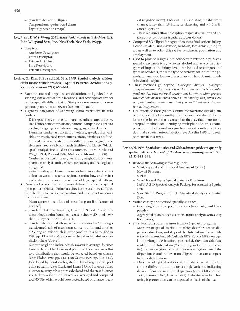
– Standard deviation Ellipses– Temporal and spatial trend charts– Layout generation (maps)

Lee, J., and D.W.S. Wong. 2001. Statistical Analysis with ArcView GIS.John Wiley and Sons, Inc., New York, New York. 192 pp.

• Chapters:– Attribute Descriptors– Point Descriptors– Pattern Detectors– Line Descriptors– Pattern Descriptors

Levine, N., Kim, K.E., and L.H. Nitz. 1995. Spatial analysis of Hon-olulu motor vehicle crashes: I. Spatial Patterns. Accident Analy-sis and Prevention 27(5):663–674.

• Examines method for geo-ref crash locations and guides for de-scribing spatial dist of crash locations, and how types of crashescan be spatially differentiated. Study area was assumed homo-geneous planar, not a network (system of roads).

• 4 general categories of analyzing spatial variations in autocrashes:– Diff types of environments—rural vs. urban, large cities vs.

small cities, state comparisons, national comparisons; tend touse highly aggregated data and large geographical units.

– Examines crashes as function of volume, speed, other vari-ables on roads, road types, intersections, emphasis on func-tions of the road system, how different road segments orelements create different crash likelihoods. Classic “black-spot” analysis included in this category (cites: Boyle andWright 1984, Persaud 1987, Maher and Mountain 1988).

– Crashes in particular areas, corridors, neighborhoods, em-phasis on analysis units, which are socially and ecologicallyintegrated.

– System-wide spatial variations in crashes (few studies on this)to look at variations across region, examine how crashes in aparticular zone or sub-area are part of larger spatial pattern.

• Developed own software to derive different indices of spatialpoint pattern (Hawaii Pointstat; cites Levine et al. 1994). Takeslist of lat/long for each crash location and produces 4 measuresof concentration– Mean center (mean lat and mean long on list, “center of

gravity”)– Standard distance deviation, based on “Great Circle” dis-

tance of each point from mean center (cites McDonnell 1979chap 1; Snyder 1987 pp. 29–33).

– Standard deviational ellipse, which calculates the SD along atransformed axis of maximum concentration and anotherSD along an axis which is orthogonal to this (cites Ebdon1985 pp. 135–141). More concise than standard distance de-viation circle (above).

– Nearest neighbor index, which measures average distancefrom each point to the nearest point and then compares thisto a distribution that would be expected based on chance(cites Ebdon 1985 pp. 143–150; Cressie 1991 pp. 602–615).Developed by plant ecologists for describing clustering ofpoint patterns (cites Clark and Evans 1954). For each point,distance to every other point calculated and shortest distanceselected, then shortest distances are averaged and comparedto a NNDist which would be expected based on chance (near-

est neighbor index). Index of 1.0 is indistinguishable fromchance, lower than 1.0 indicates clustering and > 1.0 indi-cates dispersion.

– These measures allow description of spatial variation and de-gree of concentration (spatial autocorrelation).

• Compared SD ellipses for types of crashes (fatal, serious injury,alcohol-related, single-vehicle, head-on, two-vehicle, etc.) to e/o as well as to other ellipses for residential population and employment.

• Used to provide insights into how certain relationships have aspatial dimension (e.g., between alcohol and severe injuries;types of impact and injury level), can be used to compare difftypes of accidents, the same type of accident for 2 diff time pe-riods, or same type for two different areas. These do not providebehavioral insights.

• These methods go beyond “blackspot” analysis—blackspotanalysis assumes that observation locations are spatially inde-pendent; that each observed location has its own random process,whether Poisson distributed or not. Cites Loveday and Jarrett 1992re: spatial autocorrelation and that you can’t treat each observa-tion as independent.

• Limitations to these guides: assume monocentric spatial planebut in cities often have multiple centers and these distort the re-lationships by assuming a center, but they say that there are noaccepted methods for identifying multiple nodes in a spatialplane; most cluster analyses produce biased results since theydon’t take spatial autocorrelation (see Anselin 1995 for devel-opments in this area).

Levine, N. 1996. Spatial statistics and GIS: software guides to quantifyspatial patterns. Journal of the American Planning Association62(3): 381–391.

• Reviews the following software guides:– STAC (Spatial and Temporal Analysis of Crime)– Hawaii Pointstat– S-Plus– Venables and Ripley Spatial Statistics Functions– SASP: A 2-D Spectral Analysis Package for Analyzing Spatial

Data– SpaceStat: A Program for the Statistical Analysis of Spatial

Data• Variables may be described spatially as either

– Occurring at unique point locations (incidents, buildings,people)

– Aggregated to areas (census tracts, traffic analysis zones, cityboundaries)

• Stats describing points or areas fall into 3 general categories– Measures of spatial distribution, which describes center, dis-

persion, direction, and shape of the distribution of a variable(cites Hammond and McCullogh 1978; Ebdon 1988), e.g., getlatitude/longitude locations geo-coded, then can calculatecenter of the distribution (“center of gravity” or mean cen-ter), dispersion (standard distance variation), direction of thedispersion (standard deviation ellipse)—then can compareto other distributions.

– Measures of spatial autocorrelation describe relationshipamong different locations for a single variable, indicatingdegree of concentration or dispersion (cites Cliff and Ord1981; Haining 1990; Cressie 1991). Indicates whether clus-tering is greater than can be expected on basis of chance.

150

– Measures of spatial association between two or more variables,describes the correlation or association between variables dis-tributed over space (Anselin 1992b spatial dependence article)

• STAC, DOS-based program designed by Statistical AnalysisCenter of the Illinois Criminal Justice Information Authority tohelp police depts. identify small concentrations (called “hot spotareas”) of crime.– Two modules—TIME, SPACE. SPACE module does two

things: radial search for incidents from a selected point andidentification of highest concentrations of incidents within astudy area. SPACE needs identification number and x, y lo-cation of each point in Euclidean coordinates (plane coordi-nates, UTMs). It must specify limits of study area (min/maxx, y coordinates) as well as search radius which is a circulararea that the program uses to search for points that cluster to-gether. No theoretical basis for choosing particular radii, anddifferent search radii will produce slightly different clusters.Produces ellipses to identify areas of clustering. Doesn’t havestatistic to objectively group points into unique clusters (i.e.,with fixed number of clusters and each pt assigned to one andonly one cluster).

• Hawaii Pointstat provides summary measures of the spatial dis-tribution of points. Available in DOS and Sun Unix versions,can be obtained from the Internet.– Takes list of x,y location points, can use weights/intensities

for points (i.e., if multiple WVCs occurred at same location).Distances between points calculated with 2 different metrics� Spherical geometry using “great circle” distances;� Spherical grid distances, which assume that travel occurs

only in horizontal or vertical direction (not diagonally)—used in cases of grid street systems.

– Program produces following outputs: mean center; standarddeviation of distance of each point from mean center; stan-dard deviation of ellipse (which is 2 standard deviations, onealong a transformed axis of maximum concentrations andone along an axis 90 degrees to that other axis, defining an el-lipse); nearest neighbor index; Moran’s I (Moran 1948, 1950;Ebdon 1988, Haining 1990)

– Provides summary stats of point spatial distributions and canoutput distance files for use in other programs. Useful to de-scribe distribution of points and can be used to compare dif-ferent types of distributions.

• Venables & Ripley’s Spatial Statistics Functions in S-Plus: mod-ules written in S-Plus (distributed by StatSci), available in bothUnix and Windows systems. Has Ripley’s K function utilities.Ripley’s K function uses distances between all points and com-pares the observed number of neighbors within a certain dis-tance to a theoretical number based on a Poisson randomprocess; k-fx generally considered most comprehensive of thedistance measures and can be used for determining the distancescale at which randomness occurs.

• SASP—two-dimensional spectral analysis package for analyzingspatial data—set of utility modules for conducting 2-D spectralanalysis using a grid cell organization (Renshaw and Ford 1983;Ford and Renshaw 1984; Renshaw and Ford 1984). 2-D spectralanalysis is technique for detecting patterns in a spatial distribu-tion and is direct extension of 1-D spectral analysis used in timeseries analysis.– Data consist of series of rectangular grid cells imposed over

spatial plan with m rows and n columns. The value withineach cell represents an estimate of a third variable, which

could either be number of discrete points that fall within thecell or a value attributed to the entire cell.

– “Distribution of grid cell structure can be decomposed intotrigonometric (“cyclic”) components, called a Fourier de-composition,” resulting in discrete frequencies (p & q) thatare independent of e/o and that indicate the contribution ofeach frequency to the overall pattern. Essentially an ANOVAsplitting up the variance into sine/cosine components.

– Central output is periodogram which is a plot of the sine/co-sine components and is expressed as the number of wavesdown the rows, p, and the number of waves across columns,q, with an origin at p = 0 and q = 0. Two summary indices: R-spectrum is average of periodogram values for semicircu-lar “distance” bands emanating from the origin (p = 0, q = 0)and a width of 1. The θ spectrum is an average of the peri-odogram values for an angular band (i.e., pie slices) from theorigin; that is, it is a polar coordinate band that is 10 degreeswide, starting at -5 deg -+5 deg along the x-axis and turningclockwise until 165–175 degrees.

– Also 3-D figure showing a smoothed rearranged peri-odogram.

– 2-D spectral analysis seen as exploratory guide for examiningrepeating spatial patterns.

• SpaceStat program designed to spatially analyze areal distribu-tion (Anselin 1992a), written in Gauss (matrix language). Canbe applied to data collected on individual zones or areas withina larger geographical area. – Ability to create a spatial weights file, which is a series of

weights, assigned to individual observations, indicating theirlocation in relationship to e/o. Two forms of weights:� Binary (contiguity matrix that indicates which zones are

adjacent to each other)� General (distance based matrix that indicates the relative

distance of each zone from the others. Typically defined interms of inverse distance raised to an integer power (e.g.,1/d, 1/d2, 1/d3); the higher the power of the distance fac-tor, the more “local” the effect.

– 4 modules:� First allows data to be input and transformed� 2nd involves guides for creation of spatial weights input� 3rd involves exploratory analysis including descript stats

correlations, and principal components. Includes a Join-Count statistic for binary variables and several measuresof spatial autocorrelation and descriptive model providesa local indicator of spatial association (LISA) by applyingMoran’s “I” to individual observations (Anselin 1995).

� 4th module has number of regression routines, with ordi-nary least squares (OLS) and robust method for estimat-ing OLS using a “jackknife” procedure, and provides di-agnostics to examine residuals. Includes tests for spatialautocorrelation, gauging whether spatial dist is affectingeither the distribution of the dependent variable or theresidual error terms. If no apparent spatial autocorrela-tion, then OLS is valid procedure. If there is spatial auto-correlation, then model that incorporates spatial locationneeds to be developed.�� Most regression packages don’t incorporate spatial lo-

cation and implicitly treat space as if it were random(i.e., part of the residual error term). SpaceStat onlypackage that Levine is aware of that explicitly builds lo-cation into regression procedure. While one can apply

151

non-spatial statistics to spatial data, the error associ-ated in not considering spatial location is enormous. Ineffect one is assuming that each observation is inde-pendent of all others, which is clearly wrong for spa-tially affected phenomena.

�� Author provides info on accessing all software de-scribed in article.

Levine, N. 1999. Quickguide to CrimeStat. Ned Levine and Associates,Annandale, VA.

• Guide to parallel online help menus in the program.• Eight program tabs, each with lists of routines, options and

parameters1. Primary file: point file w/x-y coordinates.2. Secondary file: optional; also point file w/ x-y cords used in

comparison with primary file.3. Reference file: “used for single and dual variable kernel den-

sity estimation.” Usually though not always a grid overlayingthe study area.

4. Measurement parametersa. Area: define area sing units (square miles, square meters,

etc.)b. Length of street network: total lengthc. Type of measurement—direct (shortest distance between

two points) or indirect (distance constrained by grid,called “Manhattan” metric).

5. Spatial distribution: provides statistics describing overall dis-tance (first order spatial stats). 3 routines for describing spatialdistance, and 2 routines for describing spatial autocorrelation(intensity variable needed for the latter two routines, weight-ing variable can also be used)—details on these routines withdescriptions are included.

6. Distance analysis: provides stats about distances betweenpoint locations, useful for identifying degree of clustering ofpoints (second order analysis). Three routines for describingproperties of the distances and two routines that output dis-tance matrices. a. m-sub:Nearest neighbor analysisb. Number of nearest neighbors c. **Linear nearest neighbor analysisd. **Number of linear nearest neighborse. **Ripley’s K statisticf. Distance matricesg. Within file point-to-point: routine outputs distance be-

tween each point in primary file to each point in second-ary file (can relate to guardrails, intersections, fencing, etc.)

7. Hotspot analysis: identifies groups of incidents clustered to-gether. Second order analysis. 3 stats:a. Nearest neighbor hierarchical spatial clustering: groups

points together on basis of spatial proximity—user definessignificance level associated with a threshold, minimumnumber of points that are required for each cluster andoutput size for displaying clusters with ellipses

b. K-means clustering routine for partitioning all points intok-groups in which K is a number assigned by the user

c. Local Moran statistics: applies to the Moran’s I statistic toindividual points or zones to asses whether particularpts/zones are spatially related to nearby points or zones

8. Interpolation tab: allows estimates of point density using thekernel density smoothing method.

• Chapter 6 hotspot analysis: – Pg 164 overview of types of cluster analyses methods

1. Hierarchical techniques: like inverted tree diagram inwhich two or more incidents are first grouped on the basisof some criteria (e.g., nearest neighbor). Then these aregrouped into second order clusters, which are thengrouped into third order clusters and this process is re-peated until either all incidents fall into a single cluster orelse the grouping criteria fails.� Literature cited: Sneath 1957; McQuitty 1960; Sokal

and Sneath 1963; King 1967; Sokal and Michener 1958;Ward 1963; Hartigan 1975

2. Partitioning techniques, or K-means technique, partitionthe incidents into a specified number of groupings, usu-ally defined by the user. All points are assigned to one(only one) group. Displayed as ellipses.� Literature cited: Thorndike 1953; MacQueen 1967; Ball

and Hall 1970; Beale 19693. Density techniques identify clusters by searching for dense

concentrations of incidents (next chapter of book dis-cusses one type of density search algorithm that uses thekernel density method.� Literature cited: Carmichael et al. 1968; Gitman and

Levine 1970; Cattell and Coulter 1966; Wishart 19694. Clumping techniques involve partitioning incidents into

groups or clusters but allow overlapping membership� Literature cited: Jones and Jackson 1967; Needham

1967; Jardine and Sibson 1968; Cole and Wishart 19705. Miscellaneous techniques: other methods less commonly

used including techniques applied to zones, not incidents.Local Moran (cites Anselin 1995)

6. Also hybrids of these methods, Block and Green 1994 usea partitioning method with elements of hierarchicalgrouping

– Optimization criteria: distinguish techniques applied tospace.1. Definition of cluster: discrete grouping or continuous

variable; whether points must belong to a cluster or can beisolated; whether points can belong to multiple clusters.

2. Choice of variables: whether weighting or intensity valuesare used to define similarities.

3. Measurement of similarity and distance: type of geometryused; whether clusters are defined by closeness or not;types of similarity measures used.

4. Number of clusters: whether there are a fixed or variablenumber of clusters; whether users can define the numberor not.

5. Scale: whether clusters are defined by small or larger areas;for hierarchical techniques what level of abstraction isconsidered optimal.

6. Initial selection of cluster locations (“seeds”): whetherthey are mathematically or user defined; specific rules todefine initial seeds.

7. Optimization routines used to adjust initial seeds into finallocations whether distance is being minimized or maxi-mized; specific algorithms used to readjust seed locations.

8. Visual display of clusters once extracted: whether drawnby hand or by geometrical object (ellipse); proportion ofcases represented in visualization.

– No single solution—different techniques will reveal differentgroupings and patterns among the groups.

152

– Chapter goes on to specifically explain Crimestat routinesand criteria for 3 techniques—hierarchical clustering basedon nearest neighbor analysis; partitioning technique basedon K-means algorithm, and zonal technique that identifieszones which are different from their nearby environment,whether they are “peaks” or “troughs”

– Discusses some advantages/limitations for some techniques:� Nearest neighbor hierarchical clustering: identify

groups of incidents where groups of incidents are spa-tially closer than would be expected on basis of chance.4 advantages1. Can identify small geographical environments

where there are concentrated incidents, useful forspecific targeting of microclimates where incidentsare occurring. Sizes of clusters can be adjusted to fitparticular groupings of points

2. Can be applied to any entire dataset and need not beapplied to smaller geographic areas, easing compar-isons between different areas

3. Linkages between several small clusters can be seenthrough second and higher order clusters—i.e.,there are different scales (geographical levels) to theclustering of points and hierarchical clustering canidentify these levels

4. Each level may imply different management strategies� Hierarchical clustering limitations

1. Size of grouping area dependent on sample size sincelower limit of mean random distance is used as cri-teria—for distributions with many incidents thresh-old will be smaller than distribution with fewer inci-dents, so not consistent definition of hotspot area

2. Arbitrariness due to minimum points rule requiringuser to define a meaningful cluster size so two differ-ent users may interpret the size of a hotspot differ-ently, also selection of p-value in the students t-dis-tance can allow variability between users. Almost allother clustering techniques have this property too.

3. No theory or rationale behind clusters. Same goesfor many other clustering techniques that are em-pirical groupings with no theory behind them; how-ever, if one is looking for a hotspot defined by landuse, activities, and targets, the technique providesno insight into why clusters are occurring or whythey could be related.

� K-means partitioning clustering: data are grouped intok groups defined by user, after specified number of seedlocations are defined by user. Routine tries to find bestpositioning of K centers and assigns each point to thecenter that is nearest. Assigns points to one and onlyone cluster, but all points are assigned to cluster, thusno hierarchy (second, higher order clusters) in routine.Basically, k-means procedure will divide the data intothe number of groups specified by the user.�� Advantages and disadvantages: Choosing too many

clusters will lead to defining patterns that don’t reallyexist whereas choosing too few will lead to poor dif-ferentiation among areas that are distinctly different.Given the numbers of clusters one chooses, the re-sults may or may not relate to actual “hotspots”

� Local Moran statistics: aggregate data by zones, appliesMoran’s I stat to individual zones allowing them to be

identified as similar or different to their nearby pattern.Basic concept: LISA local indicator of spatial associa-tion, indicator of the extent to which the value of anobservation is similar or different from its neighboringobservations. Requires two conditions: (1) each obser-vation has a variable value that can be assigned to it inaddition to its x/y coordinates; (2) the neighborhoodneeds to be defined—could be adjacent zones or allother zones negatively weighted by the distance fromthe observation zone

– Some thoughts on hotspots� 3 advantages to the 3 techniques discussed above

�� Identifies areas of high or low concentrations ofevents;

�� Systematically implements algorithms (thoughhuman decisions affect how the algorithms run); and

�� Lastly, these techniques are visual.� Disadvantages:

�� Choice of parameters in algorithms is subjective;makes this as much an art as science. Greater effect,the smaller the sample size.

�� Applies to volume of incidents, not underlying“risk.” It is an implicit density measure, but higherdensity may be a function of a higher population orrisk or both.

�� One thing to identify a concentration of incidents,but these hotspot methods don’t explain why thereis a concentration of events there. It could be ran-dom, not relate to anything inherent about the lo-cation.

�� Hotspot identification is merely an indication of anunderlying problem, but further analyses are re-quired to identify what is contributing to the occur-rences in that area.

Levine, N. 2004. CrimeStat III: Distance Analysis. Chapter 5 in: A Spa-tial Statistics Program for the Analysis of Crime Incident Loca-tions. Ned Levine & Associates: Houston, Texas, and the NationalInstitute of Justice, Washington, D.C., USA.

• First order properties are global and represent dominant patternof distribution.

• Second order (or local) properties refer to subregional patterns orneighborhood patterns within overall distribution, and tell aboutparticular environments that may concentrate crime incidents.

• NNI (nearest neighbor index):– Simple to understand, calculate ... for areas, not linear fea-

tures.– Basis of many distance statistics, some of which are imple-

mented in CrimeStat.– Compares distances between nearest points and distances

that would be expected on basis of chance and is an index thatis the ratio of two summary measures. � For each point distance to closest other point (nearest

neighbor) is calculated and averaged over all points.� Expected nearest neighbor distance if CSR = the mean

random distance. Mean random distance = d(ran) = 0.5 SQRT[A/N] whereA is area of region and n is number of points.

� NNI = d(NN)/d(ran) = ratio of observed nearest neighbordistance to mean random distance

153

�� If observed distance is same as mean random distance,then ratio will be ~1; if observed average distance issmaller than the mean random distance, then the indexwill be < 1 indicating clustering; if observed averagedistance is greater than the mean random distance,then index > 1 indicating dispersion and that points aremore widely distributed than would be expected basedon chance.

� Testing significance of NNI: Z-test to determine if signif-icant difference between observed and expected. Z =[d(NN)-d(ran)]/[SE of d(ran)]�� SE of d(ran)~ = SQRT[(4-pi)A/4pi(N-sq)] where A is

area of region and n is number of points.�� Note: significance test for NNI is not a test for CSR,

only a test of if average nearest neighbor distance is sig-nificantly different than chance, i.e., test of first ordernearest neighbor randomness. There are also second,third, and so forth order distributions that may or maynot be significantly different from CSR. All these are K-order effects.

� Edge effects can bias NNI—a point near border of studyarea may actually have its nearest neighbor on the otherside of the border, but program selects another pointwithin the study area as nearest neighbor of border point,which may exaggerate the nearest neighbor distance. Noconsensus on how to deal with this (cites Cressie 1991 foroptions) and “this version” of CrimeStat has no correc-tion for edge effects. However, bias will be significantlysmaller given datasets with clustering.

• K-order nearest neighbors: beyond nearest neighbor distances,2nd nearest neighbor, 3rd nearest, etc. In CrimeStat can specifynumber of nearest neighbor indices to be calculated. – Output includes order, starting with 1; mean nearest neigh-

bor distance for each order (m); expected nearest neighbordistance for each order (m); and NNI for each order.

– Kth NNI is ratio of observed Kth nearest neighbor distanceto the Kth mean random distance.

– CrimeStat has no test for significance (none has been devel-oped) for Kth NNI since orders aren’t independent.

– No restrictions on number of nearest neighbors that can becalculated, but since average distance increases with higherorder nearest neighbors, bias from edge effects will increase.Orders no greater than 2.5% of pts should be calculated (citesCressie 1991 pg 613 for example).

• Linear NNI (Lnna): applied to roads, with assumptions that in-direct distances are used following network or grid. – Theory: cites Hammond and McCullagh (1978). – CrimeStat calculates average of indirect distances between

each point and its nearest neighbor = Ld(NN).– Expected linear nearest neighbor distance is Ld(ran) =

0.5(L/n-1) where L is total length of road and n is sample size.– Linear NNI = LNNI = [Ld(NN)]/[Ld(ran)]– Theoretical standard error for random linear nearest neigh-

bor distance not known� Author of CrimeStat developed approx SD for observed

Ld(NN) = SLd(NN) = SQRT[Σ(min(di,j) − Ld(NN))2/N-1]where min(di,j) is nnd for point I and Ld(NN) is averagelinear nearest neighbor distance.

� SELd(NN) = [SLd(NN)]/SQRT[N] � Approx significance test = t = [Ld(NN)-Ld(ran)]/SE of

Ld(NN)

� Since empirical standard deviation of Ld(NN) used in-stead of theoretical value, t-test used rather than Z-test.

� CrimeStat output with Lnna routine:1) Sample size2) Mean linear nearest neighbor distance in meters, feet,

miles3) Minimum linear dist b/w nearest neighbors4) Maximum linear dist b/w nearest neighbors5) Mean linear random distance6) Linear nearest neighbor index7) SD of linear nearest neighbor distance8) SE of linear nearest neighbor distance9) Significance test of NNI (t-test)

• K-order linear nearest neighbors: beyond nearest neighbor dis-tances, 2nd nearest linear neighbor, 3rd nearest, etc. In Crime-Stat can specify number of nearest linear neighbor indices to becalculated. – Output includes order, starting with 1; mean linear nearest

neighbor distance for each order (m); expected linear near-est neighbor distance for each order (m); and linear NNI foreach order.

– Kth linear NNI is ratio of observed Kth linear nearest neigh-bor distance to the Kth linear mean random distance.

– Expected linear nearest neighbor distance is Ld(ran) =0.5(L/n-1) where L is total length of road and n is sample size,only adjusting for nk which occurs as degrees of freedom arelost for each successive order. Index is really the k-order lin-ear nearest neighbor distance relative to the expected linearneighbor distance for the first order—it is not a strict NNI fororders above 1.

– (*These are notes from non-linear NNI; not sure if applica-ble here, too, but there are no other notes on these issues inlinear NNI section.) CrimeStat has no test for significance(none has been developed) for Kth NNI since orders aren’tindependent.

– (*These are notes from non-linear NNI; not sure if applica-ble here, too, but there are no other notes on these issues inlinear NNI section.) No restrictions on number of nearestneighbors that can be calculated, but since average distanceincreases with higher order nearest neighbors, bias from edgeeffects will increase. Orders no greater than 2.5% of pointsshould be calculated (cites Cressie 1991 pg 613 for example).

– Example of interpreting results from higher order analyses—if one parameter shows clustering through fourth order, thentending toward more dispersed than random, then may in-dicate that there are small clusters of points, but that the clus-ters themselves are relatively dispersed; the more orders an-alyzed showing clustering, the more overall clustering acrossthe entire study area.

– Linear k-order nearest neighbor distance different than non-linear (areal). Index slightly biased as denominator (k-orderexpected linear neighbor distance) is only approximated.Also, index measures distance as if the streets follow a truegrid, oriented E/W and N/S, hence may not be realistic forplaces where streets traverse in diagonal patterns—in thesecases, use of indirect distance measurement will producegreater distances than what actually may occur on the streetnetwork.

• Ripley’s K Statistic (not for linear features—only areas)– Index of non-randomness for different scale values (cites

Ripley 1976, 1981; Bailey and Gattrell 1995; Venables and

154

Ripley 1997). “Super-order” NN statistic providing test ofrandomness for every distance from the smallest up to thesize of the study area. Sometimes called reduced second mo-ment measure implying that it is meant to measure secondorder trends (i.e., local clustering vs. general pattern over re-gion); however, also subject to first order effects so is not astrictly second order measure.

– Consider spatially random dist of n points. Circles of radius,ds, are drawn around each point, where s is the order of radiifrom smallest to largest and the number of other points thatare found within the circle are counted and then summedover all the points (allowing for duplication), then the ex-pected number of points within that radius are E(number ofpoints within distance di) = [N/A]K(ds), where N is samplesize, A is total study area, and K(ds) is area of a circle definedby ds. For example, if area defined by particular radius is 1⁄4the total study area, and if there is spatially random distribu-tion, on average approximately 1⁄4 of the cases will fall withinany one circle (+/− sampling error). More formally, withCSR, expected points within distance ds is

E(number under CSR) = [N/A] π ds2

And if average number of points found within a circle of aparticular radius placed over each point is greater than foundin above equation (expected), then clustering occurring or ifaverage number of points found within circle of particularradius placed over each point is less than found in aboveequation (expected), then dispersion.

– K statistic similar to NND because it provides info about av-erage distance b/w points, but more comprehensive thannearest neighbor distance stats for two reasons:� Applies to all orders cumulatively, not just a single order� Applies to all distances up to the limit of the study area be-

cause the count is conducted of successively increasingradii.

– Under unconstrained condition, K is defined as K(ds) =[A/N2] Σi Σj I(di,j) where I(di,j) is the number of other points,j, found within distance ds summed over all points, i. So, cir-cle of radius ds placed over each pt I, then number of otherpts ij are counted. Circle is moved to next pt i and process re-peated, thus double summation points to the count of all j’sfor each I, over all I’s. When done, radius of circle is increasedand process is completed. Typically radii of circle are in-creased in small increments so there are 50-100 intervals bywhich the statistic can be counted. In CrimeStat, 100 inter-vals (radii) are used based on ds = R/100 where R is the radiusof a circle for whose area is equal to the study area.

– Can graph K(ds) against ds to see if there is clustering at cer-tain distances or dispersion at others, but since this plot isnon linear (increasing exponentially), then transform intosq-root function L(ds) = SQRT[K(ds)/π] – ds. In practice onlythe L statistic is used even though the name of the statistic isbased on the K derivation.

– L statistic prone to edge effects, i.e., for points located nearthe boundary of the study area, the number enumerated byany circle for those points will (all other things =) be less thanpoints in the center of the study area because points outsidethe boundary aren’t counted. The > distance between pointstested (i.e., the greater the radius of the circle placed overeach point), the greater the bias, thus a plot of L vs. distancewill show decline as distance increases.

– Ripley proposed edge adjustments� “Guard rail” within study area so points outside the

guardrail but inside the study area can be counted forcenter points (an enumerator) inside the guardrail, butcannot have own circle placed upon them (i.e., only a re-cipient, can only be j’s and not I’s). Must be done manu-ally, must identify each point as either an enumerator andrecipient or recipient only. Can be problematic if studyarea boundary not “regular” shape.

� Venebles and Ripley 1997—weighting to account for pro-portion of circle placed over each point within the studyarea. Thus K(ds) = [A/N2] Σi Σj I(di,j) becomes K(ds) =[A/N2] Σi Σj Wij

−1 I(di,j) where Wij−1 is inverse of proportion

of circle of radius ds placed over each point which is withinthe total study area; thus if point is near border, it will getgreater weight because smaller proportion of circle placedover it will be within the study area. Again, has to be donemanually and can be problematic if study area boundarynot “regular” shape.

� CrimeStat only calculates the unadjusted L and tells usersto anticipate the bias by only examining L stat for smalldistances where bias is smallest (even though one couldcalculate 100 distance intervals).

– Comparison to spatially random distribution—because sam-pling distribution of L statistic not known, do 100 randomdistance simulations, then for each simulation the L statisticis calculated for each distance interval, after all simulationshave been conducted, highest/lowest L-values are taken foreach interval and is called an “envelope.” By comparing dis-tribution of L to random envelope, one can assess if observedis different from chance.� Note: since no formal test of significance, comparison

with envelope only approximate confidence aboutwhether distribution differs from chance or not, i.e., onecan’t say likelihood of obtaining this result by chance isless than e.g., 5%.

Spooner, P.G., Lunt, I.D., Okabe, A. and S. Shiode. 2004. Spatialanalysis of roadside Acacia populations on a road network usingthe network K-function. Landscape Ecology 19:491–499.

• Ripley’s K-function (Ripley 1976, 1991) not appropriate for pointpatterns on road networks since k-function assumes infinite ho-mogeneous environment for calculating Euclidean distances.

• Network k-function for univariate analyses and network crossk-function for bivariate analyses more appropriate.

• Used these methods to confirm significant clustering of Acaciapopulations at various scales and spatial patterns.

• K-function been used to study spatial patterns of mapped pointdata in plant ecology (cites a list).

• K-function uses all point-to-point distances not just nearestneighbor distances

• When k-function used for point patterns constrained by linearroad networks, can overdetect clustering patterns possibly lead-ing to Type 1 errors.

• Cites Forman 1999 ICOET article says lack of spatial guides toanalyze point patterns on road networks.

• Credits Okabe and Yamada 2001 (The k-function method on anetwork and its computational implementation. GeographicalAnalysis 33:271–290) with developing k-function analysis ofpoint patterns on a network.

155

• Refers to k-function to “reduced second moment measure” tomeasure two-dimensional distribution pattern on infinite ho-mogeneous plane where circle of radius t centered on each pointand number of neighboring points within circle are counted.Can vary radius t scale, deviation of observed from expectednumber of points plotted against t. Null hypothesis for k-func-tion is complete spatial randomness (CSR) and if observed func-tion deviates from a randomly generated (Poisson) pointprocess, the null is rejected.

• Univariate network k-function similar process but calculates theshortest path distance from each point to all other points on afinite connected planar network, assumption of binomial pointprocess based on hypothesis that points p (the set of points as-sumed on network) are uniformly and independently distrib-uted over finite road network, thus if hypothesis rejected, pointsare spatially interacting and may form non-uniform patterns.

• 100 Monte Carlo simulations used to construct confidence“envelope” based on max and min values from an equivalentnumber of random coordinates for k(t) compared to k-hat (t)or observed. Any values of k-hat (t) that lie outside confidenceenvelope were considered significant deviation from CSR. If k-hat(t) > k(t), then points p are clustered; if k-hat(t) < k(t),then points p are tending toward regularity. Edge effects aretaken into account with distance computations so no need foredge adjustment factor (Okabe & Yamada 2001)

• Bivariate network k-function, two different kinds of points A&Bare analyzed on network, with hypothesis of spatial interactionbetween different types of points. Statistical test for bivariateanalysis similar to univariate network k-function but presentversion of SANET used for network cross k-function analysesdoes not construct a confidence envelope, but can be theoreti-

cally obtained from the binomial distribution approximated bynormal distribution for large number of points. To check forstatistically significance of observed from CSR, approx of 95%CI constructed using standard deviation of normal distance, andmax/min values of +/-1.65*SD using one-sided tests. If observed> expected and outside CI, then points A&B are significantly“attracted”; if observed < expected and outside CI, then pointsA&B are significantly repelled.

• “Spatial point patterns were analyzed on a road network shape-file using SANET Version 1.0 – 021125 (Okabe et al. 2002,okabe.t.u-tokyo.ac.jp/okabelab/atsu/sanet/sanet-index.html),an ESRI Arcmap extension.” First preprocessed all polylines tomake sure properly connected to e/o. SANET used first to cal-culate distances between all notes on road network then used toassign points to the nearest point on the road network. Networkk- and cross k-function analyses were performed by SANET andoutput data were exported to Excel to aggregate data, calculateconfidence intervals (for x-k-function analyses) and producegraphs.

• Univariate addresses clustered vs. regular distributions; bivari-ate addresses if two types of sets of points are attracted orrepulsed from e/o.

• Combo of using graphical Kernel (for visual) and networkk-function was helpful, but must be realized that kernel estima-tions do not compensate for spatial differences I road networksand their effect on point patterns observed.

Final paragraph: possible applications of network k-function includeanimal movement patterns from survey and traffic mortality, en-vision network k-function becoming standard GIS application onnetworks.

156

157

Buckland et al.40 suggest that the modeling process for theanalysis of line or point transect data can be visualized as hav-ing two steps. The first involves selecting a key function as thestarting point (Figure 51), starting with the uniform or half-normal. The uniform model has no parameters,40 while thehalf-normal has one unknown parameter that has to be esti-

mated from the data. The second step is to adjust the keyfunction with a series expansion. Buckland et al.40 suggestusing (1) the cosine series, (2) simple polynomials, or (3) theHermite polynomials. All three are linear in their parame-ters.40 Given in Figure 52 are the key function and the seriesexpansion.

A P P E N D I X F

Distance Sampling

Figure 51. Functions useful in modeling distance data:(1) uniform, half-normal, and negative exponential, and (2) hazard-rate model for four different values of theshape parameter b.

Figure 52. Series expansions for adjusting key functions.

Key functions Series expansion

wUniform, 1/ Cossine, cos

Uniform, 1/ Simpl

aj y

w

w

jj

m

=∑ ⎛

⎝⎜⎞⎠⎟1

π

ee polynomial, cos

Half-nor

ay

wj

j

m j

=∑ ⎛

⎝⎜⎞⎠⎟1

2

mmal, exp Cosine, cos( / )− ⎛⎝⎜=

∑y aj y

wj

j

m2 2

2

2σ π ⎞⎞⎠⎟

−Half-normal, exp Hermite polyn( / )y2 22σ oomial,where

Hazard-ra

a H yy y

j jj

m

ss

22=

∑ ( )= / σ

tte, 1 exp Cosine, cos− − ⎛−

=∑( ( / ) )y a

j y

wb

jj

m

σ π2 ⎝⎝⎜

⎞⎠⎟

− − −Hazard-rate, 1 exp Simple p( ( / ) )y bσ lloynomial, ay

wj

j

m j

=∑ ⎛

⎝⎜⎞⎠⎟2

2

159

Table 45 shows North American terrestrial mammals scal-ing distances grouped by linear [√ HR (mi)] movement do-mains (gray-shaded column), using Ward’s linkage method

with a Euclidean distance measure to produce a hierarchicalmonothetic agglomerative clustering.162

A P P E N D I X G

Allometric Scaling

160

Common name (Genus species) HR a (ha) HR (m i 2 ) HR

(mi) MedDD b

(mi) Clustering Classes

> 11 miles c

wolverine (Gulo gulo) 150000.00 579.1500 24.07 168.46 < 11 10.71

mountain lion (Felis concolor) 29733.33 114.8004 10.71 75.00 < 10.71 > 7.15 miles

fisher (Martes pennanti ) 20342.49 78.5424 8.86 62.04 wolf (Canis lupus) 20276.88 78.2890 8.85 61.94

< 7.15 miles 3.05 miles grizzly bear (Ursus arctos) 9283.13 35.8422 5.99 41.91 coyot e (Canis latrans) 7597.57 29.3342 5.42 37.91 black bear (Ursus americana) 2413.09 9.3169 3.05 21.37

< 3.05 1.07 miles arctic fo x (Alopex lagopus) 2080.00 8.0309 2.83 19.84 lynx (Lynx canadensis) d 1852.40 7.1521 2.67 18.72 bighorn sheep (Ovis canadensis) d 1433.40 5.5344 2.35 16.47 elk (Cervus elaphus) d 1292.54 4.9905 2.23 15.64 moose (Alces alces) 1215.00 4.6911 2.17 15.16 pronghorn antelope (Antilocapra americana) 1060.47 4.0945 2.02 14.16 badger (Taxidea taxus) 849.87 3.2813 1.81 12.68 swift fox (Vulpes velox) 793.02 3.0619 1.75 12.25 antelope jackrabbit (Lepus alleni) 642.82 2.4819 1.58 11.03 prairie red fox (Vulpes vulpes fulva/regalis ) 409.76 1.5821 1.26 8.80 red fox (Vulpes vulpes) 387.34 1.4955 1.22 8.56 bobcat (Lynx rufus ) 320.82 1.2387 1.11 7.79 striped skunk (Mephitis mephitis) 294.67 1.1377 1.07 7.47

< 1.07 0.16 miles mule deer (Odocoileus hemionus hemionus) 285.27 1.1014 1.05 7.35 American marten (Martes americana) 209.31 0.8081 0.90 6.29 white-tailed deer (Odocoileus virginianus) 196.06 0.7570 0.87 6.09 black-tailed jackrabbit (Lepus californicus) 145.55 0.5620 0.75 5.25 collared peccary (Pecari tajacu) 135.21 0.5220 0.72 5.06 gray fox (Urocyon cinereoargenteus) 122.00 0.4710 0.69 4.80 long-tailed weasel (Mustela frenata) 111.29 0.4297 0.66 4.59 raccoon (Procyon lotor) 113.73 0.4391 0.66 4.64 ringtail ca t (Bassariscus astutus ) 87.75 0.3388 0.58 4.07 California black-tailed deer (Odocoileus hemionus californicus) 79.44 0.3067 0.55 3.88 black-tailed deer (Odocoileus hemionus columbianus ) 58.85 0.2272 0.48 3.34 opossum (Didelphis marsupialis) 59.88 0.2312 0.48 3.37 coati (Nasua narica) 55.00 0.2124 0.46 3.23 cotton rat (Sigmodon hispidus) 44.50 0.1718 0.41 2.90 short-tailed weasel, ermine (Mustela erminea) 20.64 0.0797 0.28 1.98 American mink (Mustela vison) 14.10 0.0544 0.23 1.63 porcupine (Erithizon dorsatum ) 11.29 0.0436 0.21 1.46 mountain western American chipmunk (Tamias quadrivittatus) 6.73 0.0260 0.16 1.13 least weasel (Mustela nivalis ) 6.75 0.0261 0.16 1.13

< 0.16 miles snowshoe hare (Lepus americanus) 5.93 0.0229 0.15 1.06 flying squirre l (Glaucomys volans/sabrinus) 4.14 0.0160 0.13 0.89 west central U.S. chipmunk (Tamias umbrinus) 4.55 0.0176 0.13 0.93 grasshopper mouse (Onychomys leucogaster) 3.62 0.0140 0.12 0.83 desert cottontail (Sylvilagus audubonii) 3.18 0.0123 0.11 0.78 western and Siberian American chipmunk (Tamias minimus) 2.10 0.0081 0.09 0.63 swamp rabbit (Sylvilagus aquaticus) 2.12 0.0082 0.09 0.63 eastern cottontail (Sylvilagus floridanus) 1.62 0.0063 0.08 0.55 pine squirrel (Tamiasciurus douglasii) 1.10 0.0042 0.07 0.46 red squirrel (Tamiasciurus hudsonicus) 1.10 0.0042 0.07 0.46 kangaroo rat (Dipodomys ordii) 1.29 0.0050 0.07 0.49 creeping vole, Oregon vole (Microtus oregoni) 0.81 0.0031 0.06 0.39 white-footed deer mous e (Peromyscus maniculatus gracilis ) 0.81 0.0031 0.06 0.39

Table 45. North American terrestrial mammals scaling distances.

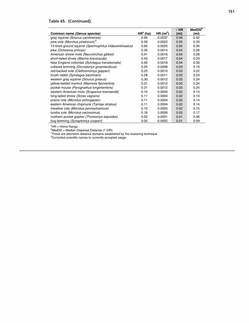
161

Common name (Genus species) HRa (ha) HR (mi2) HR

(mi) MedDDb

(mi) gray squirrel (Sciurus carolinensis) 0.95 0.0037 0.06 0.42pine vole (Microtus pinetorum) d 0.58 0.0022 0.05 0.3313-lined ground squirrel (Spermophilus tridecemlineatus) 0.66 0.0025 0.05 0.35pika (Ochotona princes) 0.35 0.0014 0.04 0.26American shrew mole (Neurotrichus gibbsii) 0.41 0.0016 0.04 0.28short-tailed shrew (Blarina brevicauda) 0.43 0.0017 0.04 0.29New England cottontail (Sylvilagus transitionalis) 0.46 0.0018 0.04 0.30collared lemming (Dicrostonyx groenlandicus) 0.20 0.0008 0.03 0.19red-backed vole (Clethrionomys gapperi) 0.25 0.0010 0.03 0.22brush rabbit (Sylvilagus bachmani) 0.28 0.0011 0.03 0.23western gray squirrel (Sciurus griseus) 0.30 0.0012 0.03 0.24yellow-bellied marmot (Marmota flaviventris) 0.31 0.0012 0.03 0.24pocket mouse (Perognathus longimembris) 0.31 0.0012 0.03 0.24western American mole (Scapanus townsendii) 0.10 0.0004 0.02 0.14long-tailed shrew (Sorex vagrans) 0.11 0.0004 0.02 0.14prairie vole (Microtus ochrogaster) 0.11 0.0004 0.02 0.14eastern American chipmunk (Tamias striatus) 0.11 0.0004 0.02 0.14meadow vole (Microtus pennsylvanicus) 0.12 0.0005 0.02 0.15tundra vole (Microtus oeconomus) 0.16 0.0006 0.02 0.17northern pocket gopher (Thomomys talpoides) 0.02 0.0001 0.01 0.06bog lemming (Synaptomys cooperi) 0.05 0.0002 0.01 0.09aHR = Home Range bMedDD = Median Dispersal Distance (7 HR)cThese are allometric distance domains established by the clustering technique dCorrected scientific names to currently accepted usage

Table 45. (Continued).

Abbreviations and acronyms used without definitions in TRB publications:

AAAE American Association of Airport ExecutivesAASHO American Association of State Highway OfficialsAASHTO American Association of State Highway and Transportation OfficialsACI–NA Airports Council International–North AmericaACRP Airport Cooperative Research ProgramADA Americans with Disabilities ActAPTA American Public Transportation AssociationASCE American Society of Civil EngineersASME American Society of Mechanical EngineersASTM American Society for Testing and MaterialsATA Air Transport AssociationATA American Trucking AssociationsCTAA Community Transportation Association of AmericaCTBSSP Commercial Truck and Bus Safety Synthesis ProgramDHS Department of Homeland SecurityDOE Department of EnergyEPA Environmental Protection AgencyFAA Federal Aviation AdministrationFHWA Federal Highway AdministrationFMCSA Federal Motor Carrier Safety AdministrationFRA Federal Railroad AdministrationFTA Federal Transit AdministrationIEEE Institute of Electrical and Electronics EngineersISTEA Intermodal Surface Transportation Efficiency Act of 1991ITE Institute of Transportation EngineersNASA National Aeronautics and Space AdministrationNASAO National Association of State Aviation OfficialsNCFRP National Cooperative Freight Research ProgramNCHRP National Cooperative Highway Research ProgramNHTSA National Highway Traffic Safety AdministrationNTSB National Transportation Safety BoardSAE Society of Automotive EngineersSAFETEA-LU Safe, Accountable, Flexible, Efficient Transportation Equity Act: A Legacy for Users (2005)TCRP Transit Cooperative Research ProgramTEA-21 Transportation Equity Act for the 21st Century (1998)TRB Transportation Research BoardTSA Transportation Security AdministrationU.S.DOT United States Department of Transportation