Evaluation of the UCL Compton camera imaging...
203
Evaluation of the UCL Compton Camera Imaging Performance Mashari A. Alnaaimi Submitted for the Degree of Doctor of Philosophy From the University College London RADIATION PHYSICS GROUP DEPARTMENT OF MEDICAL PHYSICS AND BIOENGINEERING FACULATY OF ENGINEERING SCIENCES UNIVERSITY COLLEGE LONDON July 2011 M. Alnaaimi 2011
-
Upload
truonglien -
Category
Documents
-
view
219 -
download
0
Transcript of Evaluation of the UCL Compton camera imaging...
Evaluation of the UCL Compton Camera
Imaging Performance
Mashari A. Alnaaimi
Submitted for the Degree of
Doctor of Philosophy
From the
University College London
RADIATION PHYSICS GROUP
DEPARTMENT OF MEDICAL PHYSICS AND BIOENGINEERING
FACULATY OF ENGINEERING SCIENCES
UNIVERSITY COLLEGE LONDON
July 2011
M. Alnaaimi 2011

ii
I, Mashari AlNaaimi, confirm that the work presented in this thesis is my own. Where
information has been derived from other sources, I confirm that this has been indicated in the
thesis.

iii
بسم هللا الرحمن الرحيم
In The Name Of Allah the Beneficent the Merciful

iv
Dedicated to my beloved wife and kids

v
Acknowledgments
I sincerely wish to thank my principal supervisors Dr Gary Royle and Professor Robert
Speller for the endless levels of support, advice and encouragement they have bestowed
both academically, and as friends over the duration of the course.
I greatly appreciate the support of the Radiation Physics group as the advice sought was
priceless. In particular, thanks go to Mr. Ahmad Subahi as he always brought a smile to
my face and is a sincere friend who provides a constant support both at work and in
everyday life; Mr Walid Ghoggali for his endless support and suggestions which made
my work stronger and Mr Essam Banoqitah for being extremely friendly and helpful. A
special thank you is also reserved to Dr Alassandro Olivo who unselfishly contributes to
the other individuals in the group with kind advice and knowledge; Dr. Ian Cullum for
providing me with the radioisotopes and advising me with his professional experience.
Finally, I would like to say a very special thank you to my family and especially my
parents and wife as without their constant stream of love, I could not have dreamed of
completing such a task.

vi
Publications
1. M A Alnaaimi G J Royle, W Ghoggali, and R D Speller. 2010 Development of a
pixellated germanium Compton camera for nuclear medicine 2010 IEEE Nuclear
Science Symposium Conference Record N41-150 pp 1104-1107.
2. M A Alnaaimi G J Royle, W Ghoggali, E Banoqitah, I Cullum and R D Speller
2011 Performance evaluation of a pixellated Ge Compton camera Phys. Med. Biol.
56 3473-3486 (Featured Article)
vii
Abstract
This thesis presents the imaging performance of the University College London (UCL) High
Purity Germanium (HPGe) Compton camera. This work is a part of an ongoing project to
develop a Compton camera for medical applications. The Compton camera offers many
potential advantages over other imaging modalities used in nuclear medicine. These
advantages include a wide field of view, the ability to reconstruct 3D images without
tomography, and the fact that the camera can have a portable lightweight design due to
absence of heavy collimation.
The camera was constructed by ORTEC and the readout electronics used are based on GRT4
electronics boards (Daresbury, UK). The camera comprises two pixellated germanium
detector planes housed 9.6 cm apart in the same vacuum housing. The camera has 177 pixels,
152 in the scatter detector and 25 in the absorption detector. The pixels are 4x4 mm2.
The imaging performance with different gamma-ray source energies was evaluated
experimentally and compared to the theoretical estimations. Images have been taken for a
variety of test objects including point, ring source and Perspex cylindrical phantom. The
measured angular resolution is 7.8° ± 0.4 for 662 keV gamma-ray source at 5 cm. Due to the
limited number of readout modules a multiple-view technique was used to image the source
distributions from different angles and simulate the pixel arrangement in the full camera. In
principle, the Compton camera potentially has high sensitivity but this is not recognized in
practice due to the limited maximum count rate.
Although there are a number of limitations in the current prototype camera some potentially
useful qualities have been demonstrated and distributed sources have been imaged. The key
limitations in the current prototype are acquisition time, processing time and image

viii
reconstruction. However, techniques are available to significantly improve and overcome
these limitations. This thesis presents the current state of the Compton camera performance
along with a demonstration of its strengths and limitations as a potential candidate for nuclear
medicine imaging.

Contents
ix
Contents
Abstract .............................................................................................................................. vii
Acknowledgments ............................................................................................................... iii
Publications ......................................................................................................................... vi
Contents .............................................................................................................................. ix
List of Figures ...................................................................................................................... 1
List of Tables ....................................................................................................................... 5
1 Introduction ....................................................................................................................... 8
1.1 Principle of gamma-ray imaging in Nuclear Medicine ....................................................... 8
1.2 Mechanical collimation (Gamma camera) ........................................................................ 10
1.3 Dual photons electronic collimation (PET) ...................................................................... 12
1.4 Recent advances in nuclear medicine imaging ................................................................. 16
1.5 Project motivation and aim ............................................................................................... 19
1.6 Single photons electronic collimation ............................................................................... 20
1.7 Compton Camera principle ............................................................................................... 20
1.7.1 Compton Camera potential advantages for medical imaging ..................................... 22
1.7.1.1 Sensitivity gain..................................................................................................... 23
1.7.1.2 Reconstruct 3D images without tomography ....................................................... 24
1.7.1.3 Compact and lightweight ..................................................................................... 25
1.7.1.4 Superior performance with high energy (>300 keV) ........................................... 25
1.7.2 Factors governing Compton camera performance ...................................................... 26
1.7.2.1 Angular resolution ............................................................................................... 27
1.7.2.2 Intrinsic efficiency ............................................................................................... 33
1.7.3 Development of Compton camera for medical imaging............................................. 43
1.7.3.1 Semiconductors .................................................................................................... 44
1.7.3.2 Gaseous detectors ................................................................................................. 50
1.8 Structure of Thesis ............................................................................................................ 53
1.9 Novel Work Undertaken ................................................................................................... 53
2 Materials and Methods .................................................................................................... 54
2.1 Camera geometrical design description ............................................................................ 54

Contents
x
2.2 The controlling readout electronics ................................................................................... 57
2.2.1 Moving window deconvolution (MWD) energy extraction ....................................... 61
2.2.2 Triggering and flow control ........................................................................................ 63
2.2.3 Data filtering ............................................................................................................... 66
2.3 Image reconstruction ......................................................................................................... 67
2.4 Imaging objects ................................................................................................................. 68
2.4.1 List of sources ............................................................................................................ 68
2.4.2 Achieving distributed sources .................................................................................... 70
2.4.3 Nuclear medicine phantom ......................................................................................... 72
2.4.4 Gamma camera and PET scanner specifications ........................................................ 73
2.5 Multiple views setup ......................................................................................................... 74
2.6 Data analysis ..................................................................................................................... 77
Point spread function (PSF) ................................................................................................... 77
Signal to noise ratio (SNR) ................................................................................................ 77
Percentage contrast ............................................................................................................ 78
2.7 Image acquisition .............................................................................................................. 78
2.8 Errors................................................................................................................................. 79
2.9 Previous Characterisation ................................................................................................. 80
2.9.1 Position sensitivity...................................................................................................... 80
2.9.2 Simulated efficiency ................................................................................................... 83
3 Results and Discussions .................................................................................................. 85
3.1 Probability of interaction .................................................................................................. 85
3.1.1 With the absorption (back) detector ........................................................................... 88
3.1.2 Random coincidence in Compton camera .................................................................. 91
3.2 System performance characterises .................................................................................... 97
3.2.1 Energy resolution........................................................................................................ 97
3.2.2 Angular resolution .................................................................................................... 101
3.2.2.1 Energy resolution contribution........................................................................... 101
3.2.2.2 Geometry contribution ....................................................................................... 102
3.2.3 Point source images .................................................................................................. 104
3.2.3.1 Limited geometry images .................................................................................. 104
3.2.3.2 Multiple views images ....................................................................................... 109
3.2.3.3 Deconvoluted point source image ...................................................................... 116
3.2.4 Distance dependence ................................................................................................ 118
3.2.5 Efficiency ................................................................................................................. 120
3.2.6 Timing properties ..................................................................................................... 121

Contents
xi
3.2.6.1 Time resolution .................................................................................................. 121
3.2.6.2 Time window width vs. image quality ............................................................... 124
3.2.6.3 CFD parameter optimization .............................................................................. 125
3.2.7 Counting limitation ................................................................................................... 128
3.2.7.1 Effect of activating more pixels ......................................................................... 129
3.2.7.2 Effects of photons flux ....................................................................................... 131
3.3 Distributed source images ............................................................................................... 133
3.3.1 Cs137
Line source ...................................................................................................... 133
3.3.2 Cs137
circular source ................................................................................................. 135
3.3.3 Ring source ............................................................................................................... 137
3.4 Resolving power ............................................................................................................. 140
3.5 Phantom images .............................................................................................................. 142
3.5.1 F18
triangles phantom imaging ................................................................................. 142
3.5.2 I131
imaging ............................................................................................................... 146
3.5.2.1 I131
triangle phantom images .............................................................................. 146
3.5.2.2 I131
vial imaging .................................................................................................. 149
3.5.2.3 I131
Disk shape source ......................................................................................... 152
3.6 Comparison with gamma camera and PET ..................................................................... 154
3.6.1 PET images ............................................................................................................... 155
3.6.2 Gamma camera planar images .................................................................................. 159
4 Conclusions and Future Work ...................................................................................... 164
4.1 Summary ......................................................................................................................... 164
4.2 Conclusions ..................................................................................................................... 165
4.3 Future work ..................................................................................................................... 173
Appendix .......................................................................................................................... 177
Bibliography .................................................................................................................... 183
Chapter 1. Introduction
1
List of Figures
Figure 1: The basic component of a gamma camera. ..................................................................... 11
Figure 2: A photograph of a PET system (The Siemens Biograph mCT). The detectors form a ring
around the patient to detect the annihilation gamma ray pairs. .............................................. 14
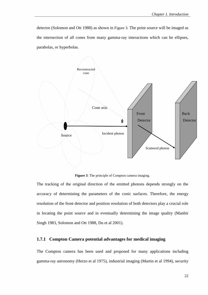
Figure 3: The principle of Compton camera imaging. ................................................................... 22
Figure 4: Principle of 3 dimensional image reconstruction of Compton camera. .......................... 25
Figure 5: the key performance parameters for Compton camera ................................................... 26
Figure 6: the probability of single photon scatter Pc for Ge and Si with different gamma energies
(Singh 1983). .......................................................................................................................... 36
Figure 7: Example of a preamplifier output trace fed to an oscilloscope along with a sketch of a
fast leading edge and a slow exponantial tail. ........................................................................ 39
Figure 8: A photograph of the UCL pixellated Ge Compton camera along with a description of its
detectors geometry. ................................................................................................................ 55
Figure 9: Cross-section of the camera highlighting the precise diameter and components of the
camera. ................................................................................................................................... 56
Figure 10: preferred Compton scatter angles at 662 keV............................................................... 57
Figure 11: A photograph of the GRT4 readout electronics (a), the outline of one GRT4 card VME
module (b) .............................................................................................................................. 58
Figure 12: the UCL Compton camera and GRT readout electronics components ......................... 59
Figure 13: The principle of operation for the pixellated Ge Compton camera .............................. 60
Figure 14: the original signal measured from a preamplifier (top) and the deconvoluted signal
trapezoid shape (bottom) following the application of MWD routine. The total charge
deposited by the photon interaction is calculated as the average value between the start and
the end of the flat top of the deconvoluted pulse (Descovich 2002). ..................................... 61
Figure 15: sketch of the MWD algorithm pulse parameters .......................................................... 62
Figure 16: common dead time operation (I H Lazarus 2006) ........................................................ 64
Figure 17: block diagram of the intended improved GRT4 readout system .................................. 65
Figure 18: propeller attached to a rotating motor ........................................................................... 70
Figure 19: a photograph of the I131
vial placed below the camera front detector (a) and a schematic
of the distributed source location with respect to the positions of the front active pixels. .... 71
Figure 20: the experiment setup in air (left) and water (right). ...................................................... 71
Figure 21: Photographs of the triangles phantom design ............................................................... 73
Chapter 1. Introduction
2
Figure 22: (a) A bottom view for the camera with a map of the front and back pixels. The point
source position for the multi-view acquisition is indicated by the yellow dots (b) the rotating
platform used for multiple views imaging. ............................................................................ 76
Figure 23: example of the induced charge in neighbouring pixels with positive polarity ............. 81
Figure 24: position sensitivity of the system can be defined within 2 mm3 voxel ........................ 82
Figure 25: simulated efficiency of the UCL Compton camera for a point source at 5 cm from the
front camera face (G J Royle et al 2003). .............................................................................. 83
Figure 26: Compton cross section and Compton/Total cross section ratio for Si, Ge, and CZT
(Wernick and Aarsvold 2004). ............................................................................................... 87
Figure 27: The measured front, back, and total energy deposited in the camera by a 662 keV
source. .................................................................................................................................... 90
Figure 28: Types of coincidence events in Compton camera; true events (left) and random events
(right). .................................................................................................................................... 93
Figure 29: (a) photograph of the experiment setup with lead brick to shield the back detector (b)
sketch of the setup with the expected path of the photons ..................................................... 94
Figure 30: Cs137
point images acquired with and without shielding the back detector pixels. ...... 95
Figure 31: Energy calibration linearity curve for a front pixel (CR11) based on Ba133
and Cs137
photopeaks. ............................................................................................................................ 98
Figure 32: The energy resolution pixels map along with the FWHM table for the NIM analogue
electronics (top) and the GRT4 electronics (bottom) obtained with 662 keV source. ........... 99
Figure 33: The FWHM value energy vs. the MWD window width. The bars represents the
standard errors. ..................................................................................................................... 100
Figure 34: Limited geometry point source images acquired with different source energies (a) 356
keV, (b) 511 keV, and (c) 662 keV. The cross indicates the nominal source position. ....... 106
Figure 35: The experimental measured FWHM (mm) for 356, 511, and 662 keV. The R2 suggests
a good fit. ............................................................................................................................. 108
Figure 36: point source images acquired from different angles ................................................... 110
Figure 37: The 8 views superimposed point source image (a) a photograph of the point source
used in this experiment (diameter =2 mm). ......................................................................... 111
Figure 38: horizontal and vertical line profiles taken through the centre of the single and multiple
view images.......................................................................................................................... 112
Figure 39: A source with 2 mm diameter of uniform intensity (100 arbitrary units) give a
measured image in which part of signal is seen outside actual source. Note that the intensity
of measured image is reduced to 85 (Soret et al 2007). ....................................................... 114
Figure 40: The original backprojected point source image (a) the Deconvoluted point (b) and the
difference image(c) along with the line profile taken through each image. ......................... 117
Chapter 1. Introduction
3
Figure 41: PSF (mm) vs. distance from the front detector (cm), the error bars was obtained by
taking the standard error of the mean FWHM values which is 2mm. The R2 suggests a good
fit. ......................................................................................................................................... 119
Figure 42: coincident counts collected as a function of channel number. Time window with 75
and 12.5 ns width were projected on the time axis .............................................................. 122
Figure 43: SNR (arbitrary unit) for different time window widths (ns) ....................................... 125
Figure 44: The SNR obtained with different CFD values. The error bars was obtained by taking
the standard error of the mean value. ................................................................................... 126
Figure 45: images reconstructed with different CFD discriminator levels. ................................. 127
Figure 46: DTR vs. the number of back pixels used to trigger the front. The error bars represents
the standard errors. ............................................................................................................... 129
Figure 47: Front pixels used with fixing the back pixels to 4 pixels vs. DTR (Mbytes/sec). The
error bars are the standard errors. ......................................................................................... 131
Figure 48: The DTR vs. the incident photons flux. The error bars represents the standard errors.
.............................................................................................................................................. 132
Figure 49 : Cs137
line source backprojected image(a) backprojected image with correction (c, e,
and f) horizontal line profile at y= 12.25, 11.25 and 10.25 cm respectively for (a) and the
same line profiles for (b) are presented in(d, g, and h) ........................................................ 135
Figure 50: circular source with 1.5 cm diameter reconstructed with backprojection (a) and its
corresponding line profile (b)............................................................................................... 136
Figure 51: Multiple views for a circular source distribution acquired at 0,90,180, and 270 degrees
from the camera central axis ................................................................................................ 137
Figure 52: The summed image for a circular source with different diameters 1.5, 2, and 3 cm
respectively. ......................................................................................................................... 138
Figure 53: Line profiles taken through the center of the 1.5, 2, and 3 cm diameters ring image
respectively. ......................................................................................................................... 138
Figure 54: Two points separated by 3.5 mm backprojection image (a) and its corresponding
profile (b). ............................................................................................................................ 141
Figure 55: Multiple views for the phantom acquired at 0, 90,180, and 270 degrees from the
camera central axis. .............................................................................................................. 143
Figure 56: the 4 views backprojected summed image for the F18
triangles phantom .................. 143
Figure 57: Line profiles taken through (a) the top row, (b) the middle row and (c) the bottom row.
.............................................................................................................................................. 144
Figure 58: the F18
triangles phantom after applying a correction factor to the top and bottom rows.
Note the recovered top and bottom intensity compared to Figure 56. ................................. 145
Figure 59: Line profiles taken through (a) the top row, (b) the middle row and (c) the bottom row
with applying a correction factor for the top and bottom rows. ........................................... 145

Chapter 1. Introduction
4
Figure 60: I131 triangle summed four views image. ................................................................... 147
Figure 61: Line profiles taken through (a) the top row, (b) the middle row and (c) the bottom row.
.............................................................................................................................................. 148
Figure 62: the corrected line profiles taken through (a) the top row, (b) the middle row and (c) the
bottom row. .......................................................................................................................... 148
Figure 63: The vial image in air (a) water (b) with horizontal line profile through the centre of the
image in air(c) and water (d) ................................................................................................ 150
Figure 64: The disk shape image in air (a) water (b) with horizontal line profile through the centre
of the image in air(c) and water (d) ...................................................................................... 153
Figure 65: the triangles phantom fused PET/CT image (a) and PET image (b). The A letter inside
the box is an indicator for the Anterior view ....................................................................... 156
Figure 66: Line profiles taken through (a) the top row, (b) the middle row and (c) the bottom row.
.............................................................................................................................................. 156
Figure 67: the triangles phantom imaged with Compton camera (a) and PET (b) ...................... 157
Figure 68: I131
planar gamma camera image reconstructed with 40,000 counts .......................... 159
Figure 69: Line profiles taken through (a) the top row, (b) the middle row and (c) the bottom row.
.............................................................................................................................................. 160
Figure 70: The triangles phantom filled with I131 (10MBq/tube) imaged by Compton system with
38,000 events (a) and gamma camera with 1900 events(b) along with the horizontal line
profiles for Compton camera image (c) and gamma camera(d) ........................................... 162

Chapter 1. Introduction
5
List of Tables
Table 1: The performance characteristics of typical commercially available parallel-hole
collimators . ............................................................................................................................ 12
Table 2: The spatial resolution and sensitivity of some of the commercially available PET
systems. .................................................................................................................................. 14
Table 3: physical properties of semiconductors of importance in selecting front detector
materials.*value at 77 K temperature (Knoll 1999, Scannavini et al 2000, Dedek et al 2008).
................................................................................................................................................ 40
Table 4: The performance characteristics of the most interesting designs of medical Compton
imaging camera. ..................................................................................................................... 52
Table 5: the MWD algorithm setting parameters used with the GRT4 readout electronics. ......... 62
Table 6: The radioisotopes used in this project along with their properties and images obtained for
them. The numbers between brackets represents the percent yield per decay. ...................... 69
Table 7: properties of water (tissue) and Perspex.* the mass and linear attenuation coefficient is at
662 keV. ................................................................................................................................. 72
Table 8: the PET acquisition parameters used to acquire the images. ........................................... 74
Table 9: Theoretical calculation of the front detector energy as a function of scatter angle with
different source energies ........................................................................................................ 86
Table 10: interaction probabilities for different energy sources placed 10 cm from the front
detector pixels. ....................................................................................................................... 88
Table 11: the theoretically expected no. of photons interacts with the back detector (1cm) and
probability of PE and CS for different source energies. ........................................................ 89
Table 12: the electron momentum, the contribution of energy resolution, the contribution of
Doppler broadening and the angular uncertainty due to Doppler broadening for 360 and 663
keV source energy. ............................................................................................................... 102
Table 13: Summary of the calculated factors that contribute to the overall angular resolution using
in Singh’s quadratic equation for a 662 keV source placed at 5 cm. ................................... 104
Table 14: The experimental (Exp) measured and the theoretically calculated (theory) angular and
spatial resolution at 5 cm from the camera. The error in the measurement is half the pixel
size (± 2mm). ....................................................................................................................... 107
Table 15: Quantitative comparison between multiple and single view images at 3 cm. ............. 113
Table 16: Variation of spatial resolution with the number of camera views. .............................. 116
Table 17: The time window widths (ns) vs. the SNR and the number of counts collected. The
standard error was taken for the result. The standard error (± 0.2) was taken for the SNR. 124

Chapter 1. Introduction
6
Table 18: summary of the total count and SNR for different CFD threshold levels, the threshold
voltage can be converted to threshold energy since 9 mV equals 60 keV (Lazarus 2004). . 126
Table 19: The SNR and Contrast for the single and multiple views images ............................... 139
Table 20: The horizontal profile FW2/3, FWHM, and FWTM values for the single and multiple
view images.......................................................................................................................... 151
Table 21: The SNR and contrast for image in air and water. ....................................................... 152
Table 22: The FWHM, signal to noise ratio and contrast for the I131 image in air compared to
water. .................................................................................................................................... 153
Table 23: The true, random, and scatter count rates .................................................................... 155
Table 24 : The measured SNR and % contrast for Compton camera and PET images ............... 158
Table 25: The SNR and % contrast for Compton camera vs. gamma camera ............................. 161

Chapter 1. Introduction
7
List of Abbreviations
a.u. Atomic unit
Ba Barium
BD Back detector
BP Back projection
Cm Centimetre
Cs Cesium
CT Computed tomography
E Energy
FD Front detector
FPGA Field-Programmable Gate Array
FWHM Full Width Half Maximum
FWTM Full Width tenth Maximum
HEGP High Energy General Purpose
keV Kilo-electron volts
LEGP Low Energy General Purpose
LOR Line of response
MLEM Maximum likelihood expectation maximisation
mm Millimetre
MRI Magnetic Resonance Imaging
Na Sodium
NECR Noise equivalent count rate
NIST National institute of standards and technology
PET Positron emission tomography
PSF Point spread function
SNR Signal to noise ratio
SPECT Single photon emission tomography
UCL University College London
Chapter 1. Introduction
8
Chapter 1
1 Introduction
1.1 Principle of gamma-ray imaging in Nuclear Medicine
Nuclear Medicine is a very important branch of medical imaging which utilizes gamma-
ray emitting radionuclide to obtain information about the physiology of the organs within
the human body as well as the detection of tumour growth sites. This is done by
introducing the radioactive labelled substance into the patient body and placing the
patient around external radiation detectors. These radioactive labelled substances, which
are called radiotracers, can then be used to track physiological processes in vivo typically
imaged using a gamma camera (Sorenson and Phelps 1987).
The radiotracers participate in the biochemical or physiological processes in the body in
the same way as the non-radioactive material. Since the emitted γ-rays from the
radioactive material can be detected by an external camera, radiotracers may be used to
track the flow or distribution of analogs of natural substances in the body.
There are two major types of radiotracers used: single photon emitters and positron
emitters. Single photon emitters may emit one principal gamma ray or a sequence of
gamma-rays that are directionally uncorrelated. On the other hand, positron emitters emit
a positron that travels a short distance and annihilates with an electron. This annihilation
generates two 511keV gamma rays, which travel in opposite directions.
Chapter 1. Introduction
9
Gamma camera uses mechanical collimators to project the γ-rays from single photon
emitters onto the scintillation detector to have a one-to-one spatial correlation between
points of emission and detection to accurately form the image. This is done by allowing
only photons travelling in a specific direction to be detected otherwise they will be
absorbed by the collimator before reaching the detector. The gamma camera 3-
dimensional imaging mode is called the Single Photon Emission Computed Tomography
(SPECT). SPECT is an extension of planar gamma camera imaging. The three-
dimensional distributions of radiotracers within the body are estimated from a set of two-
dimensional projection images acquired by planar cameras from a number of views
surrounding the patient more details will be discussed in section 1.2.
The PET scanner is used to image radio-nuclides that decay by positron emission. The
positron combines with an electron resulting in emission of a pair of gamma-rays
travelling in opposite directions as will be discussed in (section 1.3).
There are many limitations in SPECT and PET. The spatial resolution of SPECT images
deteriorates with high energy radioisotopes where the detection efficiency and spatial
resolution becomes low due to the collimator design and NaI crystal limitation. Moreover,
because of the heavy lead collimator gamma camera is practically difficult to be portable.
The main limitations of PET are the high cost and the almost exclusive dependence on
cyclotron produced short half-life radioisotopes. Therefore, it is very important to develop
alternative methods for gamma-rays imaging that can be used to image positron emitters
with lower costs. Compton camera is a promising imaging technique that can be used to
provide an alternative for PET and SPECT providing a portable imaging system for high
energy (>300 keV) radioisotopes.
Chapter 1. Introduction
10
In the UCL effort is on the go to produce a pixellated high purity germanium (HPGe)
Compton camera imaging system for medical application to overcome some of gamma
camera and PET limitations. The motivation is to develop a compact portable imaging
system to image gamma-ray emissions in nuclear medicine examinations with high spatial
resolution and detection sensitivity. In this work the aim is to present and quantitatively
evaluate the imaging performance of the UCL Compton camera and compare it to other
systems currently used in nuclear medicine in order to bring into focus its potential
benefits in this field.
This chapter describes the principle, applications, and limitations of imaging modalities
used in nuclear medicine. In addition, the Compton camera principle, advantages, and a
literature review for the most significant contributions in this field are presented in this
chapter.
1.2 Mechanical collimation (Gamma camera)
The most commonly used imaging instrument in nuclear medicine is the gamma camera
which was developed by Anger (1958). The gamma camera makes use of a scintillation
crystal, which is usually made of NaI(Tl), optically coupled to a photomultiplier tubes
(PMTs). The gamma camera makes use of collimators to project the gamma rays from the
source distribution onto the scintillation detector to have a one-to-one spatial correlation
between points of emission and detection for accurate image formation. This is done by
allowing only photons travelling in a certain direction to be detected otherwise they will
be absorbed by the collimator before reaching the detector. The gamma rays are
converted into flashes of light by the NaI(Tl) crystal which is then transformed to
electronic signals by the PMTs. The output of the PMTs is then converted into three
signals: (X and Y) that give the spatial location of the scintillation and (Z) which gives
Chapter 1. Introduction
11
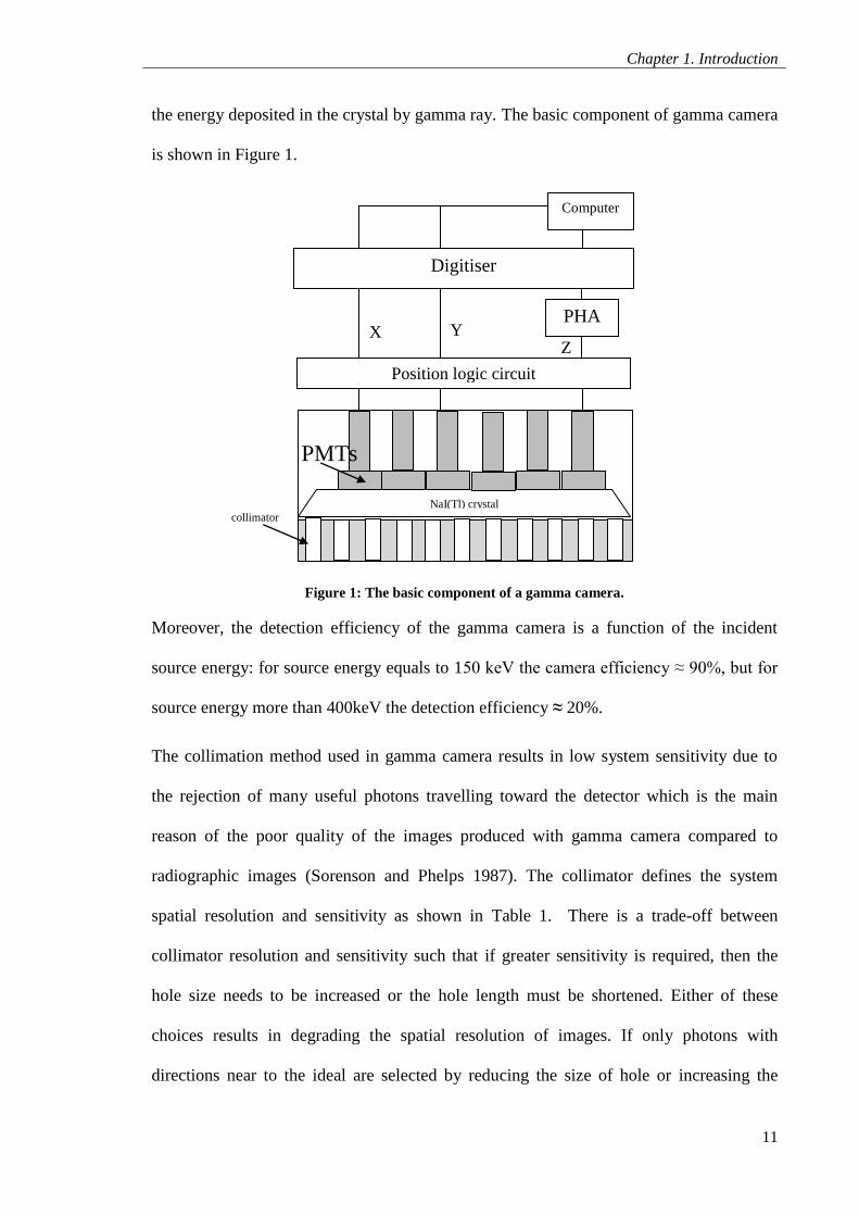
the energy deposited in the crystal by gamma ray. The basic component of gamma camera
is shown in Figure 1.
Figure 1: The basic component of a gamma camera.
Moreover, the detection efficiency of the gamma camera is a function of the incident
source energy: for source energy equals to 150 keV the camera efficiency ≈ 90%, but for
source energy more than 400keV the detection efficiency ≈ 20%.
The collimation method used in gamma camera results in low system sensitivity due to
the rejection of many useful photons travelling toward the detector which is the main
reason of the poor quality of the images produced with gamma camera compared to
radiographic images (Sorenson and Phelps 1987). The collimator defines the system
spatial resolution and sensitivity as shown in Table 1. There is a trade-off between
collimator resolution and sensitivity such that if greater sensitivity is required, then the
hole size needs to be increased or the hole length must be shortened. Either of these
choices results in degrading the spatial resolution of images. If only photons with
directions near to the ideal are selected by reducing the size of hole or increasing the
NaI(Tl) crystal
Position logic circuit
PHA
Computer
Digitiser
Z Y X
PMTs
collimator
Chapter 1. Introduction
12
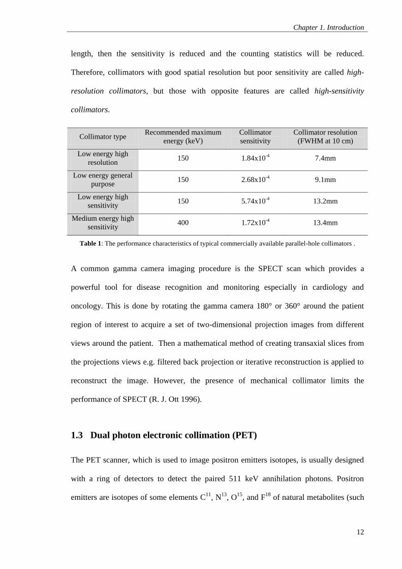
length, then the sensitivity is reduced and the counting statistics will be reduced.
Therefore, collimators with good spatial resolution but poor sensitivity are called high-
resolution collimators, but those with opposite features are called high-sensitivity
collimators.
Collimator type Recommended maximum
energy (keV)
Collimator
sensitivity
Collimator resolution
(FWHM at 10 cm)
Low energy high
resolution 150 1.84x10
-4 7.4mm
Low energy general
purpose 150 2.68x10
-4 9.1mm
Low energy high
sensitivity 150 5.74x10
-4 13.2mm
Medium energy high
sensitivity 400 1.72x10
-4 13.4mm
Table 1: The performance characteristics of typical commercially available parallel-hole collimators .
A common gamma camera imaging procedure is the SPECT scan which provides a
powerful tool for disease recognition and monitoring especially in cardiology and
oncology. This is done by rotating the gamma camera 180° or 360° around the patient
region of interest to acquire a set of two-dimensional projection images from different
views around the patient. Then a mathematical method of creating transaxial slices from
the projections views e.g. filtered back projection or iterative reconstruction is applied to
reconstruct the image. However, the presence of mechanical collimator limits the
performance of SPECT (R. J. Ott 1996).
1.3 Dual photon electronic collimation (PET)
The PET scanner, which is used to image positron emitters isotopes, is usually designed
with a ring of detectors to detect the paired 511 keV annihilation photons. Positron
emitters are isotopes of some elements C11
, N13
, O15
, and F18
of natural metabolites (such
Chapter 1. Introduction
13
as glucose, water, and ammonia). For that reason, it is possible to label biological carriers
without changing their structure and behaviour. PET provides a great diagnostic means
for many medical applications including cardiology, neurology, and oncology. A
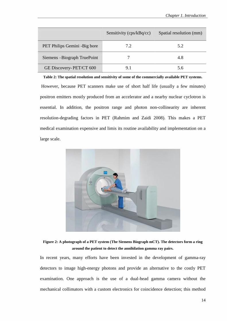
photograph of a Siemens Biograph PET system is shown in as shown in Figure 2.
The first positron emitter imaging was carried out in the early fifties by (Brownell and
Sweet 1953) with NaI(Tl) detector. Since then, different detectors types and numbers
have been used for the PET system. Most of PET scanners nowadays are accompanied by
a CT scanner in the same machine to be used for the attenuation correction and to provide
information about the structural anatomy to provide a better diagnosis (M Pennant et al
2010). Originally, PET scanners have utilised bismuth germinate (BGO) scintillation
crystals arranged into ring arrays. Many new dense scintillators with high speed and light
output like LSO and LaBr3 have been used to improve the performance of PET scanners
(Daube-Witherspoon et al 2010, Bisogni et al 2011)
The image acquisition is based on the external detection of the 511 keV two annihilation
photons, as a coincidence event. A true annihilation event requires a coincidence timing
window (typically 4.5 nanoseconds) between two detectors on opposite sides of the
scanner, hence “electronic collimation”. For accepted coincidences, lines of response
(LOR) connecting the coincidence detectors are drawn through the object and used in the
image reconstruction. This method of detection achieves higher sensitivity and improved
image quality compared to mechanically collimated gamma camera (Alberto Del Guerra
and Belcari 2007). The spatial resolution of PET scanner depends on the type, size and
the geometrical configuration of the detector elements. The spatial resolution and
sensitivity of some commercially available PET scanners is presented in Table 2. In
addition, the absence of mechanical collimators and the ring design let the field of view of
the camera to cover large area (Rahmim and Zaidi 2008).
Chapter 1. Introduction
14
Sensitivity (cps/kBq/cc) Spatial resolution (mm)
PET Philips Gemini -Big bore 7.2 5.2
Siemens –Biograph TruePoint 7 4.8
GE Discovery- PET/CT 600 9.1 5.6
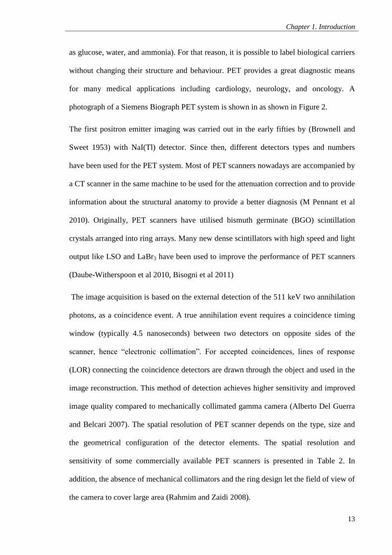
Table 2: The spatial resolution and sensitivity of some of the commercially available PET systems.
However, because PET scanners make use of short half life (usually a few minutes)
positron emitters mostly produced from an accelerator and a nearby nuclear cyclotron is
essential. In addition, the positron range and photon non-collinearity are inherent
resolution-degrading factors in PET (Rahmim and Zaidi 2008). This makes a PET
medical examination expensive and limis its routine availability and implementation on a
large scale.
Figure 2: A photograph of a PET system (The Siemens Biograph mCT). The detectors form a ring
around the patient to detect the annihilation gamma ray pairs.
In recent years, many efforts have been invested in the development of gamma-ray
detectors to image high-energy photons and provide an alternative to the costly PET
examination. One approach is the use of a dual-head gamma camera without the
mechanical collimators with a custom electronics for coincidence detection; this method
Chapter 1. Introduction
15
is called the dual-headed coincidence imaging (DHCI). This method has improved the
spatial resolution and sensitivity of the gamma camera (Patton and Turkington 1999).
However, the sensitivity of the DHCI is lower than the PET system and is not sufficient to
anatomically locate the uptake of the positron emitter in the body in a short acquisition
time (Bergström et al 2010).
Another interesting approach is the use of Multi-wire proportional chambers (MWPCs)
which have been used as a position sensitive charged particle detector in nuclear and
high-energy physics (R. J. Ott 1993). MWPCs are large-area gas-filled ionization
chambers in which large arrays of fine wires are used to determine the position of
ionization produced in the gas by the passage of charged particles. Each wire functions as
an individual ionization detector in their simplest form the anode and cathode planes. The
main advantages of MWPCs are the high-count-rate performance, large area, high spatial
resolution and low cost (Ott 1993). Several groups have worked on the development of
MWPC detectors for positron emission tomography (Bateman et al. 1980; A. Del Guerra
et al. 1988). Intrinsically the gas ionisation chambers have a very low efficiency for
detecting gamma rays unless photon-electron convertor is incorporated. Lead is used as a
convertor and proved to significantly increase the detection efficiency for 511 keV
photons with minimal effect on the spatial resolution of the detector. A large area MWPC
camera (MUP-PET) was installed in the Royal Marsden Hospital in Sutton and has been
used successfully to measure the radiation dose to the thyroid (R. J. Ott et al. 1987). In
addition, this system was used to plan targeted radionuclide therapy that was done by
imaging I124
mIBG to provide treatment planning information for therapies of neural crest
tumors with I131
mIBG (R. J. Ott et al. 1992) .
The main drawbacks of MWPCs are the low detection efficiency for 511 keV photons
and the high minimum usable coincidence window (~30 ns) which lead to increase the
Chapter 1. Introduction
16
effect of scattered photons (Ott 1993). Nevertheless, the development of a hybrid system
of barium fluoride (BaF2) scintillating crystals and MWPCs has shown great promise to
overcome problems of sensitivity and timing resolution (K Wells et al 1994). This hybrid
system retains the large area and high spatial resolution of the gaseous detectors but has
10 to 15 times improved sensitivity and a factor of 3 improved timing resolutions; thus,
make it perfectly suited for the pre-therapy tracer studies and therapy planning based on
pharmacokinetics (R. J. Ott 1996). Recently, Divoli et al. (2005) reported the
improvement of this hybrid camera which has a spatial resolution of 7.5 mm, a timing
resolution of 3.5 ns, and a total coincidence count-rate performance of at least 80–90
kcps. Preliminary phantom and patient images was presented. The count-rate
performance is limited by the read-out electronics and computer system and the
sensitivity by the use of thin (10 mm thick) crystals. These limitations are being addressed
to improve the performance of the camera.
1.4 Recent advances in nuclear medicine imaging
This section summaries the performance and the recent ongoing development of the two
main nuclear medicine studies namely the gamma camera SPECT imaging and PET.
Their capabilities in terms of sensitivity and spatial resolution as well as their limitations
will be presented to gain a better understanding of their impact on clinical practice. The
ongoing developments are focusing mainly in enhancing the performance of PET and
SPECT in terms of optimizing the hardware design (e.g. slit, slant, and pinhole
collimators), software development (e.g. resolution modelling and compensation,
dynamic image reconstruction), and data correction techniques (e.g. attenuation, random,
scatter, partial volume, and motion correction) as discussed in (Rahmim and Zaidi 2008,
Wells et al 2007, Wells et al 2010).
Chapter 1. Introduction
17
In SPECT, many approaches were carried out to optimize and develop novel collimator
designs in order to increase the sensitivity. For example, Lodge et al (1996) and
(Vandenberghe et al 2006) used a rotating slat instead of holes collimator which has
larger solid angle of acceptance. Another approach used a smaller field of view (FOV) to
gain sensitivity by using converging-hole collimator. One example is the use of rotating
multi-segment slant-hole (RMSSH) collimators (Wagner et al 2002). The RMMSH
collimators improved the sensitivity by a factor of 2 along with the additional advantage
of achieving complete angle tomography with few camera positions, depending on the
number of segments in the collimator. Thus, this technique is very useful for SPECT
mammography (Brzymialkiewicz et al 2005). Another exciting example is the use of
pinhole collimator to acquire SPECT images which has improved the spatial resolution to
sub-millimetre scale, but at the expense of system sensitivity (Beekman and Have 2006).
To compensate for the sensitivity loss multi-pinhole collimators have been proposed and
used by (Vastenhouw and Beekman 2007).
Another area of increasing interest is the simultaneous dual-tracer SPECT imaging which
is done by simultaneous imaging of different isotopes energies with multiple energy
windows (Rahmim and Zaidi 2008). For example, the use of Tc99m
(140 keV) sestamibi
stress scan and Tl201
(75 and 167 keV) rest myocardial perfusion imaging which results in
reducing the acquisition time and increase the patient comfort. The problem of using this
approach is the presence of crosstalk between the multiple energy windows. Current
research is working on optimising the parameters of the multiple energy-windows (Jong
et al 2002).
Moreover, the use of attenuation correction in SPECT is becoming increasingly important
(Heller 2004) since the tissue thickness varies with different depths or regions within the
patient body. Therefore, lack of attenuation correction can produce errors (artefacts) in
Chapter 1. Introduction
18
the reconstructed images and affect the quantitative accuracy of SPECT imaging. The
introduction of the combined SPECT/CT scanners provides a convenient fast
measurement of the X-rays transmission data that can be used for attenuation correction
(Blankespoor et al 1996). However, the use of dual-modality system has introduced some
artefacts like the misregistration of emission and transmission data due to the respiratory
motion artefact (Goetze et al 2007), truncation artefact due to the discrepancies in the
fields of view, and beam-hardening artefact caused by the polychromatic nature of the X-
ray (Hsieh et al 2000). Recently, researchers are focusing on developing methods to
compensate for these artefacts in statistical reconstruction methods (Zaidi and B
Hasegawa 2003).
In PET, with the advances in technology and statistical reconstruction algorithms the
factors that limit the resolution namely the positron range and photon non-collinearity can
be modelled in the reconstruction task to further improve the reconstructed images
resolution (Selivanov et al 2000). Moreover, the feasibility of improving PET resolution
by application of strong magnetic field, which reduces the positron range, has been
verified by (Christensen et al 1995). This approach has increased the interest in designing
a combined PET/MRI system which is a potential very powerful technique (Pichler et al
2006).
It is worth noting that the development of fast scintillators such as lutetium
oxyorthosilicate (LSO), lutetium yttrium oxyorthosilicate (LYSO) and Lanthanum three
bromide (LaBr3) have permitted the coincidence timing window to be reduced to 2 ns
compared to (10 -12 ns) with conventional bismuth germinate (BGO) scanners (Derenzo
et al 2003, Moses 2003). This improvement will reduce the random events rate and
improve the count rate performance in PET scanners. In addition, researches are ongoing
to develop faster readout electronics e.g. the use of avalanche photodiodes (APDs) to
Chapter 1. Introduction
19
replace the bulky PMTs due to their high quantum efficiency, internal gain and
insensitivity to magnetic field (Shah et al 2004, Pichler et al 2006). Also, silicon
photomultipliers (SiPMs), which is a finely pixellated APD, became recently available
commercially from several manufacturers and is potentially a promising candidate for use
as photodetectors in PET (Moehrs et al 2006, Dolgoshein et al 2006).
With the constant improvements in the electronics and fast scintillators, the time-of-flight
(ToF) PET ,which can measure the difference of the arrival times of the two annihilation
photons, was recently reconsidered (Moses 2003, Conti et al 2005). Encoding the ToF
information can potentially reduce statistical noise variance and improve the
reconstruction of PET images. The first commercially available (ToF) PET scanner was
produced by Philips medical systems manufacturer and its performance was presented in
(Surti et al 2007).
In order to produce accurate quantitative data some corrections are very important to PET
data like: random event corrections, scatter corrections, partial volume effect correction,
and motion correction. These corrections are a subject of ongoing research in PET
imaging (Rahmim and Zaidi 2008).
1.5 Project motivation and aim
The Compton camera is a promising imaging system that can be used to provide
an alternative for gamma camera and PET scanner and offers a portable imaging
device.
The motivation of this project is to develop a portable Compton camera to be used
in nuclear medicine with high spatial resolution and detection sensitivity.
Chapter 1. Introduction
20
The main aim of this project is to present and evaluate the imaging performance
of the UCL pixellated Ge Compton camera and compare it to other cameras used
in nuclear medicine to determine its potential benefits.
1.6 Single photons electronic collimation
Todd et al (1974), firstly, proposed the principle of using gamma camera to detect
Compton scattered photons. The idea was to replace the conventional absorptive
mechanical collimator with a second detector which works as an electronic collimation
for the scattered photons by recording two photons detected within the preset time
window which is called coincidence events.
In 1983, Singh and Doria built the first laboratory Compton camera device for medical
use (M. Singh 1983; M. Singh & Doria 1983). They replaced the gamma camera
mechanical collimator with a germanium detector which served as the front (scatter)
detector of Compton camera and the NaI crystals of the gamma camera as the back
(absorption) detector. This camera was evaluated and compared to the performance of the
conventional gamma camera with mechanical collimation (M. Singh & Doria 1985).
After the pioneering work of Singh and Doria many Compton camera designs and
different detector types have been proposed and tested. The basic principle, applications,
and potential advantages of Compton camera as well as a review of the literature will be
presented in the following section.
1.7 The Principle of Compton Camera
A Compton camera is a type of gamma camera that makes uses of the kinematics of
Compton scatter to build the image without using mechanical collimators. The
mechanical collimator is replaced with a second detector which works in coincidence
Chapter 1. Introduction
21
with the first detector and electronically collimates the incident photons. A Compton
camera is designed usually with two planar detectors and a specific distance is placed
between them to choose a preferred range of scatter angles.
In a Compton imaging system, the incident photons interact with the first detector and
Compton scatters from an electron in the detector. The scattered photon is then absorbed
in the second detector. A Compton imaging system, therefore, decouples the trade-off
between spatial resolution and detection efficiency that characterizes a conventional
collimated gamma camera.
A cone, see figure 3, will be defined from each photon emission, if this photon interacts
with the first detector by one Compton interaction and the scattered photon is then
photoelectrically absorbed or deposits part of its energy in the second detector. The
location of source is defined by backprojecting and intersecting all conic surfaces from
many emitted photons in the image space. Hence, the likely position of the source can be
somewhere on the surface of a cone, which creates serious uncertainty in the
reconstruction (K Iniewski 2009). The cone semi-angle is the Compton scatter angle, thus
if the source energy is known the angle between the incident and the scattered gamma ray
photon direction can be determined from the energy of recoil electron measured in the
front detector as given by (1.
(1)
where moc2
is the electron rest mass (0.511 MeV), Eγ is the source energy and Ere is the
recoil electron energy. The line that joins the two points of the interaction in the two
detectors, defines the cone axis and the cone apex is at the scattering point in the front
Chapter 1. Introduction
22
detector (Solomon and Ott 1988) as shown in Figure 3. The point source will be imaged as
the intersection of all cones from many gamma-ray interactions which can be ellipses,
parabolas, or hyperbolas.
Figure 3: The principle of Compton camera imaging.
The tracking of the original direction of the emitted photons depends strongly on the
accuracy of determining the parameters of the conic surfaces. Therefore, the energy
resolution of the front detector and position resolution of both detectors play a crucial role
in locating the point source and in eventually determining the image quality (Manbir
Singh 1983, Solomon and Ott 1988, Du et al 2001).
1.7.1 Compton Camera potential advantages for medical imaging
The Compton camera has been used and proposed for many applications including
gamma-ray astronomy (Herzo et al 1975), industrial imaging (Martin et al 1994), security
Front
Detector
Back
Detector
Source
Reconstructed
cone
Cone axis
Scattered photon
Incident photon
Chapter 1. Introduction
23
applications (Dedek et al 2008), and medical imaging (M. Singh 1983). In this thesis the
medical application of the Compton camera will be investigated.
The Compton camera offers many potential advantages for nuclear medicine application.
These advantages include the increased sensitivity which results in an improved signal-to-
noise ratio, shorter counting times, and reduced patient dose. In addition, the absence of
heavy mechanical collimators permits the Compton camera to be designed in a compact
portable setup that can be used to image high energy gamma-rays (>300 keV) with high
spatial resolution and sensitivity. The principle of image reconstruction in Compton
camera can be utilized to reconstruct 3D images without the need to acquire tomographic
images. The following sub-sections summaries the potential advantages of Compton
camera.
1.7.1.1 Sensitivity gain
In principle, the Compton camera provides better sensitivity than gamma camera due to
the absence of the mechanical collimators and the wide field of view that results in using
larger fraction of photons emitted from the source to reconstruct the image (G W Phillips
1995). The sensitivity gain with Compton camera is about 15 to 20 times better than the
mechanical collimators in 140 to 511 keV energy range (Han and Clinthorne 2009). In
theory, this could result in a reduction of both the administrated dose to the patient and
the scanning time, thus, achieving an increase in patient comfort and minimizing the
patient motion artefacts. However, practically the effect of noise in the image
reconstruction process can reduce the sensitivity gain as discussed by (M. Singh et al.
1988; Bolozdynya et al. 1997). In addition, the energy dynamic range for Compton
camera is very wide, in comparison with PET or SPECT, due to the absence of
mechanical collimator. Thus, the Compton camera can be used for simultaneous multi-
energy imaging as reported by (S. Kabuki et al 2006). Unlike gamma-camera there is no
Chapter 1. Introduction
24
trade-off between resolution and sensitivity, thus fulfilling the two main requirements for
emission medical imaging (LeBlanc et al 1998). Compared to the Compton imaging
system, a conventional gamma camera system with lead collimator imposes a trade-off
between resolution and sensitivity because of the physical constraints resulting from the
mechanical collimation. As the imaged γ-ray photons exceed ~250keV, the collimator
septal thickness must be increased to reduce the penetration and scattering of higher
energy photons in the collimator material. Because the sensitivity for a fixed hole size
collimator is reduced as the square of septal thickness, resolution must be sacrificed by
increasing hole size if sensitivity is to be maintained.
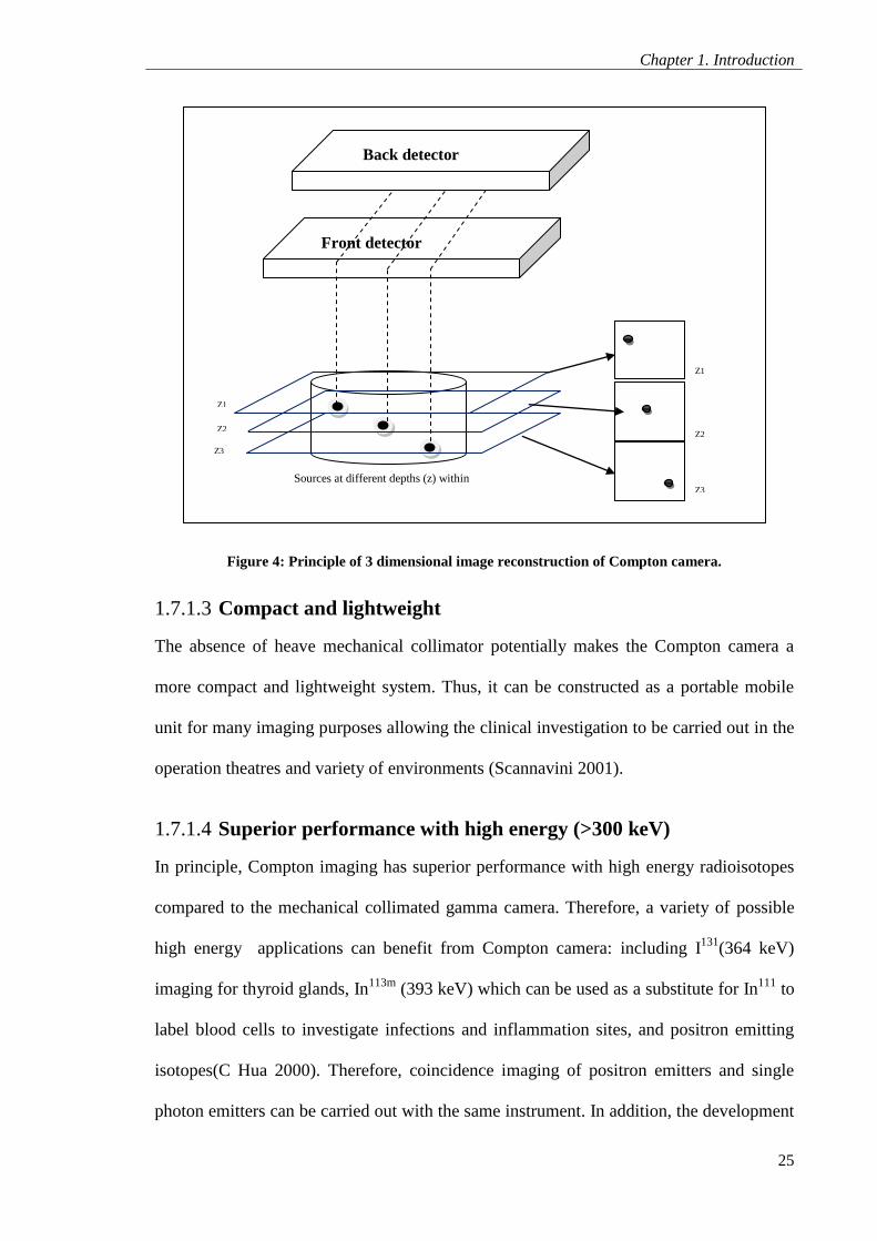
1.7.1.2 Reconstruct 3D images without tomography
The concept of image reconstruction in Compton camera allows images to be
reconstructed at different depths from a single shot without tomography and without
moving the patient as shown in Figure 4. Thus, 3-dimensional images can be reconstructed
with a more simplified system design and setup that allow the camera to be positioned
closer to the patient ( Phillips 1995).
Chapter 1. Introduction
25
Figure 4: Principle of 3 dimensional image reconstruction of Compton camera.
1.7.1.3 Compact and lightweight
The absence of heave mechanical collimator potentially makes the Compton camera a
more compact and lightweight system. Thus, it can be constructed as a portable mobile
unit for many imaging purposes allowing the clinical investigation to be carried out in the
operation theatres and variety of environments (Scannavini 2001).
1.7.1.4 Superior performance with high energy (>300 keV)
In principle, Compton imaging has superior performance with high energy radioisotopes
compared to the mechanical collimated gamma camera. Therefore, a variety of possible
high energy applications can benefit from Compton camera: including I131
(364 keV)
imaging for thyroid glands, In113m
(393 keV) which can be used as a substitute for In111
to
label blood cells to investigate infections and inflammation sites, and positron emitting
isotopes(C Hua 2000). Therefore, coincidence imaging of positron emitters and single
photon emitters can be carried out with the same instrument. In addition, the development
Z1
Z2
Z3
Z1
Z2
Z3
Back detector
Front detector
Sources at different depths (z) within
the imaged object
Chapter 1. Introduction
26
of Compton camera could facilitate the development of new physiological tracers for
different diagnostic applications based on radioactive elements that have not been
considered suitable currently because of their high energy radiation.
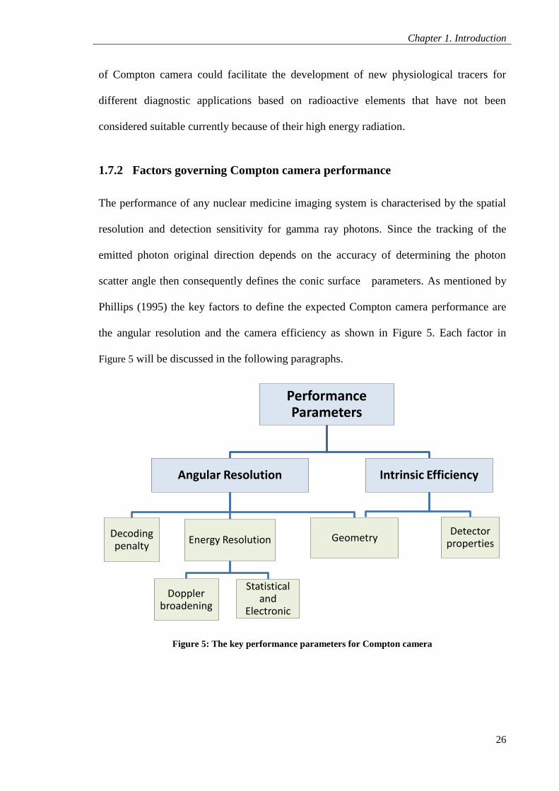
1.7.2 Factors governing Compton camera performance
The performance of any nuclear medicine imaging system is characterised by the spatial
resolution and detection sensitivity for gamma ray photons. Since the tracking of the
emitted photon original direction depends on the accuracy of determining the photon
scatter angle then consequently defines the conic surface parameters. As mentioned by
Phillips (1995) the key factors to define the expected Compton camera performance are
the angular resolution and the camera efficiency as shown in Figure 5. Each factor in
Figure 5 will be discussed in the following paragraphs.
Figure 5: The key performance parameters for Compton camera
Performance Parameters
Angular Resolution
Decoding penalty
Energy Resolution
Doppler broadening
Statistical and
Electronic
Geometry
Intrinsic Efficiency
Detector properties
Chapter 1. Introduction
27
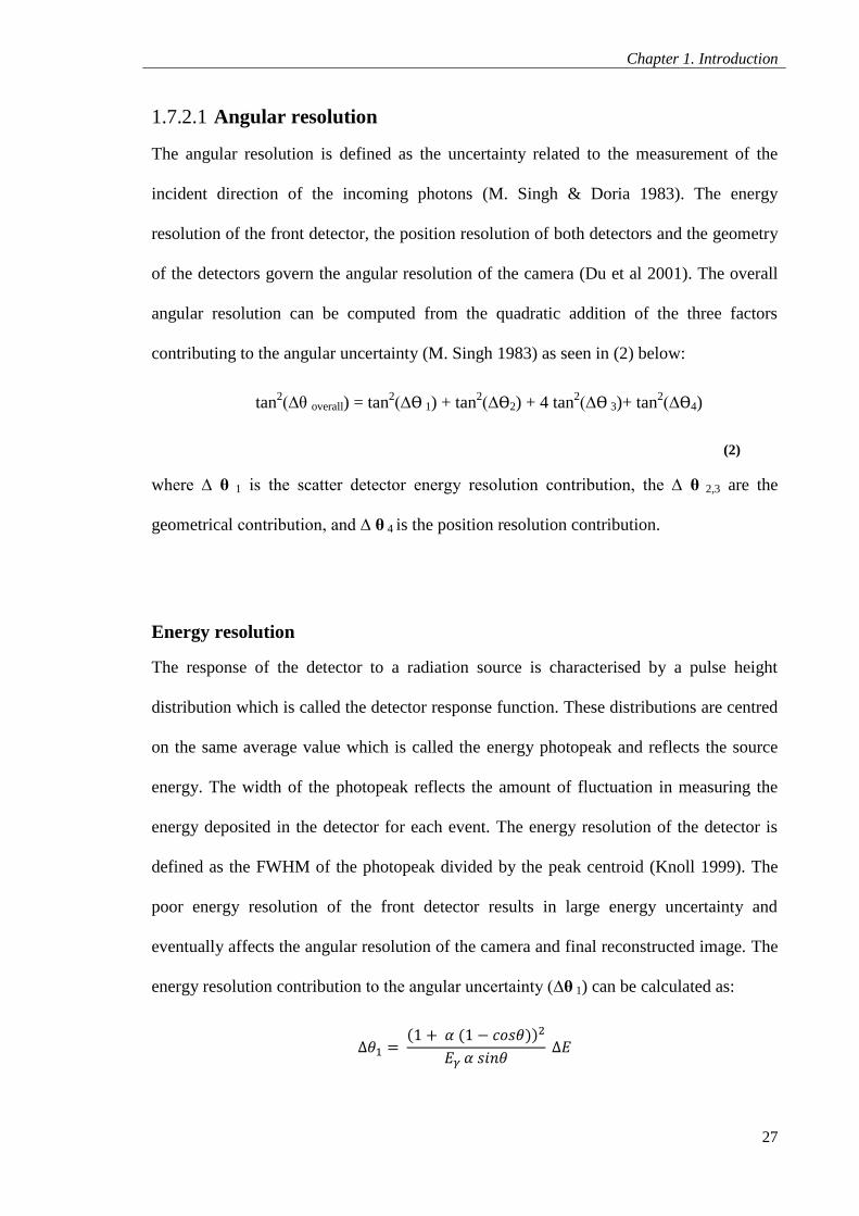
1.7.2.1 Angular resolution
The angular resolution is defined as the uncertainty related to the measurement of the
incident direction of the incoming photons (M. Singh & Doria 1983). The energy
resolution of the front detector, the position resolution of both detectors and the geometry
of the detectors govern the angular resolution of the camera (Du et al 2001). The overall
angular resolution can be computed from the quadratic addition of the three factors
contributing to the angular uncertainty (M. Singh 1983) as seen in (2) below:
tan2(∆θ overall) = tan
2(∆Ѳ 1) + tan
2(∆Ѳ2) + 4 tan
2(∆Ѳ 3)+ tan
2(∆Ѳ4)
(2)
where ∆ θ 1 is the scatter detector energy resolution contribution, the ∆ θ 2,3 are the
geometrical contribution, and ∆ θ 4 is the position resolution contribution.
Energy resolution
The response of the detector to a radiation source is characterised by a pulse height
distribution which is called the detector response function. These distributions are centred
on the same average value which is called the energy photopeak and reflects the source
energy. The width of the photopeak reflects the amount of fluctuation in measuring the
energy deposited in the detector for each event. The energy resolution of the detector is
defined as the FWHM of the photopeak divided by the peak centroid (Knoll 1999). The
poor energy resolution of the front detector results in large energy uncertainty and
eventually affects the angular resolution of the camera and final reconstructed image. The
energy resolution contribution to the angular uncertainty (∆θ 1) can be calculated as:
Chapter 1. Introduction
28
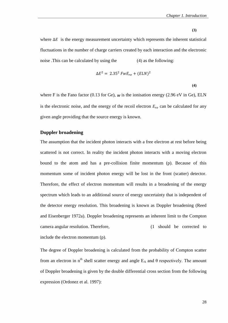
(3)
where is the energy measurement uncertainty which represents the inherent statistical
fluctuations in the number of charge carriers created by each interaction and the electronic
noise .This can be calculated by using the (4) as the following:
(4)
where F is the Fano factor (0.13 for Ge), w is the ionisation energy (2.96 eV in Ge), ELN
is the electronic noise, and the energy of the recoil electron can be calculated for any
given angle providing that the source energy is known.
Doppler broadening
The assumption that the incident photon interacts with a free electron at rest before being
scattered is not correct. In reality the incident photon interacts with a moving electron
bound to the atom and has a pre-collision finite momentum (p). Because of this
momentum some of incident photon energy will be lost in the front (scatter) detector.
Therefore, the effect of electron momentum will results in a broadening of the energy
spectrum which leads to an additional source of energy uncertainty that is independent of
the detector energy resolution. This broadening is known as Doppler broadening (Reed
and Eisenberger 1972a). Doppler broadening represents an inherent limit to the Compton
camera angular resolution. Therefore, (1 should be corrected to
include the electron momentum (p).
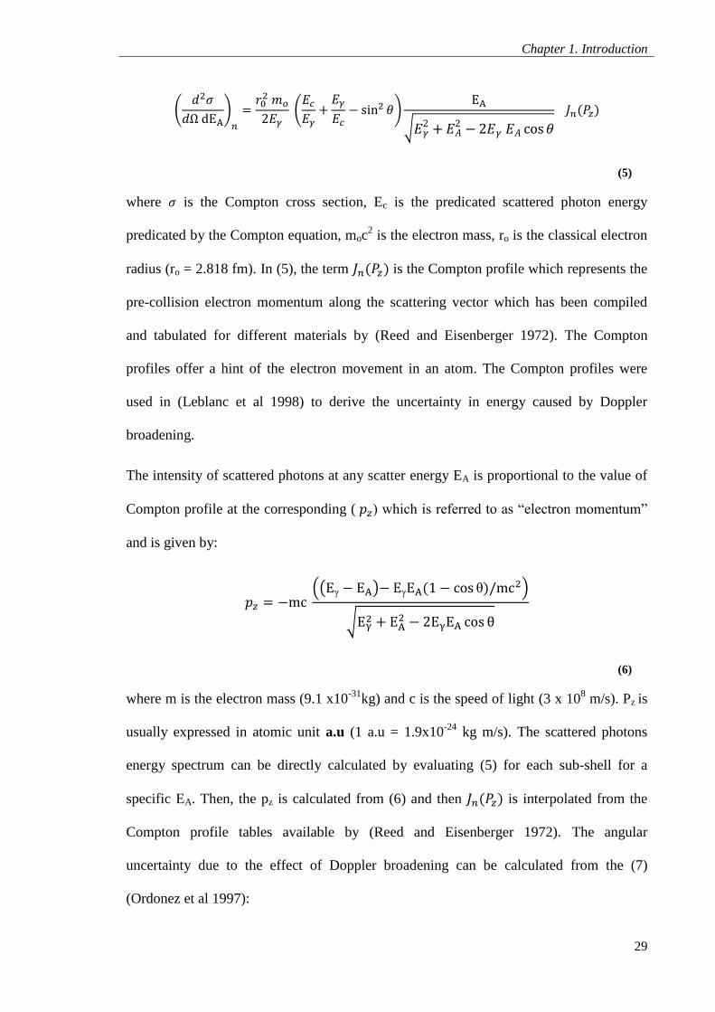
The degree of Doppler broadening is calculated from the probability of Compton scatter
from an electron in nth
shell scatter energy and angle EA and θ respectively. The amount
of Doppler broadening is given by the double differential cross section from the following
expression (Ordonez et al. 1997):
Chapter 1. Introduction
29
(5)
where is the Compton cross section, Ec is the predicated scattered photon energy
predicated by the Compton equation, moc2 is the electron mass, ro is the classical electron
radius (ro = 2.818 fm). In (5), the term is the Compton profile which represents the
pre-collision electron momentum along the scattering vector which has been compiled
and tabulated for different materials by (Reed and Eisenberger 1972). The Compton
profiles offer a hint of the electron movement in an atom. The Compton profiles were
used in (Leblanc et al 1998) to derive the uncertainty in energy caused by Doppler
broadening.
The intensity of scattered photons at any scatter energy EA is proportional to the value of
Compton profile at the corresponding ( ) which is referred to as “electron momentum”
and is given by:
γ γ θ
(6)
where m is the electron mass (9.1 x10⁻³¹
kg) and c is the speed of light (3 x 10⁸ m/s). Pz is
usually expressed in atomic unit a.u (1 a.u = 1.9x10⁻²⁴
kg m/s). The scattered photons
energy spectrum can be directly calculated by evaluating (5) for each sub-shell for a
specific EA. Then, the pz is calculated from (6) and then is interpolated from the
Compton profile tables available by (Reed and Eisenberger 1972). The angular
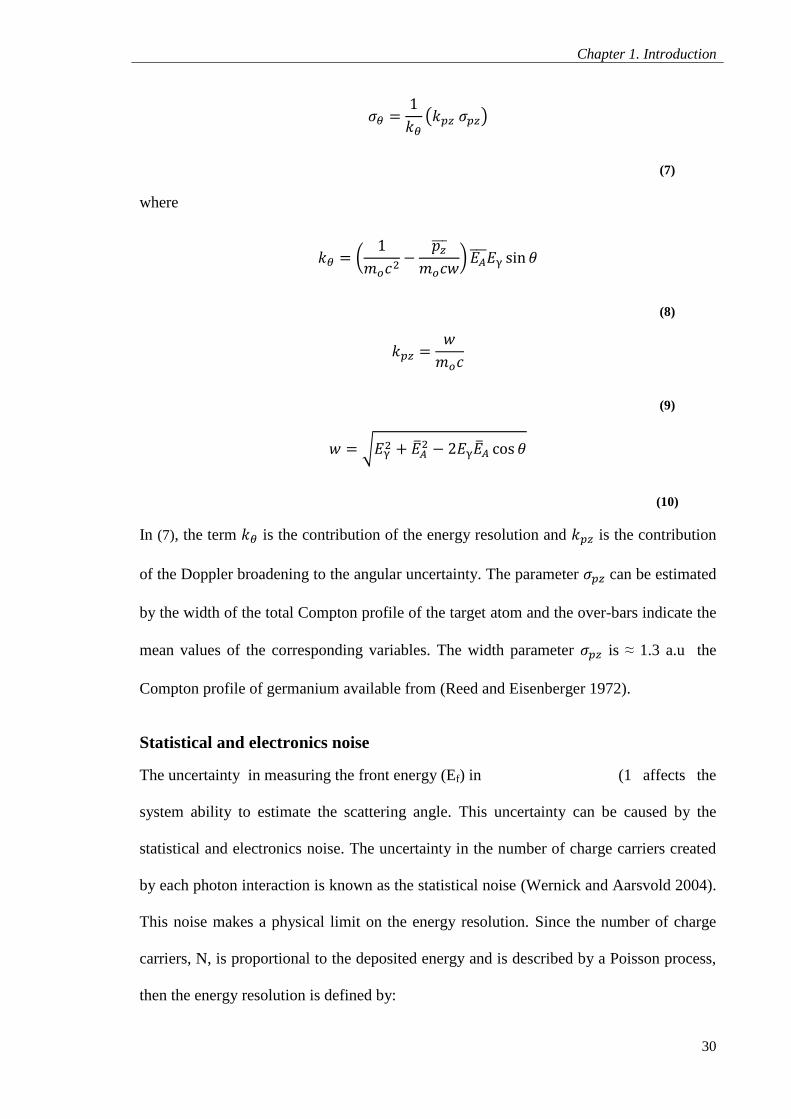
uncertainty due to the effect of Doppler broadening can be calculated from the (7)
(Ordonez et al 1997):
Chapter 1. Introduction
30
(7)
where
(8)
(9)
(10)
In (7), the term is the contribution of the energy resolution and is the contribution
of the Doppler broadening to the angular uncertainty. The parameter can be estimated
by the width of the total Compton profile of the target atom and the over-bars indicate the
mean values of the corresponding variables. The width parameter is ≈ 1.3 a.u the
Compton profile of germanium available from (Reed and Eisenberger 1972).
Statistical and electronics noise
The uncertainty in measuring the front energy (Ef) in (1 affects the
system ability to estimate the scattering angle. This uncertainty can be caused by the
statistical and electronics noise. The uncertainty in the number of charge carriers created
by each photon interaction is known as the statistical noise (Wernick and Aarsvold 2004).
This noise makes a physical limit on the energy resolution. Since the number of charge
carriers, N, is proportional to the deposited energy and is described by a Poisson process,
then the energy resolution is defined by:
Chapter 1. Introduction
31
(11)
However, in fact the process is not Poisson and the initial recoil electron energy is divided
between electron-hole pair production and other energy loss mechanisms. The ratio of
the observed variance in N to the predicted by Poisson model is known as the Fano factor.
The electronics noise in the detector readout is usually expressed as the equivalent noise
charge (ENC) at the input of the preamplifier. The ENC is defined as the amount of
charge that would give rise to an output voltage equal to the root mean square level of the
output due only to noise (Knoll 1999).
Detectors geometry
The geometry of the Compton camera detectors plays an important role in determining
the interaction positions and choosing the range of the scattering angles. Any change in
the camera geometry will affect the position uncertainty of the camera. As explained by
(M. Singh & Doria 1983) the angular uncertainty due to the geometry contribution is
inversely proportional to the square of the distance between the front and back detectors.
To calculate ∆Ѳ 2,3,and 4 which represents the effect of geometry and position resolution on
the overall angular resolution in (2) the following formulas (M. Singh 1983) are used:
(12)
(13)
(14)
Chapter 1. Introduction
32
where S is the separation between the detectors, d and L are the front pixel width and
thickness respectively, Φ is the half angle subtended by a pixel in the front detector, and r
is the FWHM position resolution of the back detector (Singh 1983). The effect of
geometry on the angular resolution of the Compton camera was calculated and will be
presented in (section 3.2.2.2).
Reconstruction decoding penalty
Compton cameras include computationally costly decoding (reconstruction) calculations
and noise propagation during the decoding phase. The reconstruction of Compton camera
images is complicated due to the lack of a physical collimator, thus, the angular resolution
due to measurement errors can vary from event to event (Parra 2000). Since the
interaction of the backprojected cone and the source plane is not a straight line as in
SPECT, the reconstructed Compton camera image exhibits artefacts that degrades the
image spatial resolution. As a result, the intensity information in the reconstructed image
does not reflect accurately the source activity distribution (Du et al 2001). In addition,
reconstructing distributed sources is difficult and can be ineffective due to the inherent
geometrical complexity of Compton camera data image (Andreyev et al 2011). Image
reconstruction of Compton camera images has to overcome many difficulties, such as the
large amount of data, noise arising from both low counts recorded and imaging response.
Several approaches were proposed to develop an efficient reconstruction method for
Compton cameras as discussed in section 2.3 and compensate for resolution loss. For
instance, analytical approaches that can compensate for the resolution degradation and
improve the spatial resolution of the reconstructed images by modelling the factors that
contribute to the angular uncertainty and include it in the reconstruction task was
proposed by (Hirasawa and T Tomitani 2004).
Chapter 1. Introduction
33
A mathematical model, based on the uniform Cramer-Rao bound, was used by (C H Hua
et al 1999) to measure the information loss during the reconstruction stage. Their model
showed that the decoding penalty degradation effect is significant especially with
extended source distributions and with low source energy due to Doppler broadening
effect.
Another approach based on statistical image reconstructions (OSEM) that includes a
resolution recovery technique was proposed by Kim et al (2010). This method considered
a Gaussian resolution model for the inherent angular and geometric uncertainties which
were incorporated into the OSEM reconstruction algorithm. The results showed that this
method improved the image spatial resolution by an order of magnitude (Kim et al 2010).
However, these methods are based on simulated data and validating these results with
real data is needed.
1.7.2.2 Intrinsic efficiency
The efficiency of any radiation detector is a combination of two factors; geometric
(absolute) and intrinsic efficiency. The geometric efficiency is ratio of the number of
photons emitted by the source to the number of useful signals detected in the camera.
Whereas, the intrinsic efficiency of a radiation detector is defined as the fraction of the
gamma rays striking the detector which results in useful signals in the detector (G F
Knoll. 1999). The intrinsic Compton camera efficiency is defined as the fraction of
photons entering the first detector that undergo only one Compton scattering and are then
photoelectrically absorbed in the second detector (Du et al 2001) and is expressed as:
(15)
Chapter 1. Introduction
34
Where Ω1 is the solid angle subtended by the front detector at the source, ΔΩ1 is the solid
angle for a differential volume element dV1 in the front detector, Ω2 is the solid angle
subtended by the back detector at the interaction position in the front detector, L1 is the
attenuation length in the front detector between the source and dV1, L12 is the attenuation
length between the two elements dV1 and dV2, µc, µp and µt are the Compton,
photoelectric, and the total linear attenuation coefficients respectively, and
is the
Klein-Nishina Compton scattering angular cross-section per electron (G F Knoll. 1999).
As indicated in Figure 5 in (section 1.7.2) the intrinsic Compton camera efficiency
depends on the detector geometries. The front and back detector geometries defines the
solid angles Ω1 and Ω2 in (15).
The efficiency is determined by the energy of the photons, system geometry and detector
martial. In fact, the interaction probabilities, energy deposition in both detectors, and
intervals between emitted photons are random process, thus, it is very complicated to
estimate the efficiency by a simple calculation. Therefore, a Monte Carlo program
(EGS4) was used by Royle et al (2003) to calculate the UCL Compton camera efficiency
(εicc) for a point source at 5 cm from the front detector surface and the result is presented
in (section 2.9.2).
Detector properties
Many types of detectors were considered for the construction of the Compton camera like
scintillators, gaseous detectors, and semiconductors. Semiconductors are the best
candidate for their excellent energy resolution due to the larger number of charge carriers
created by each incident radiation photon.
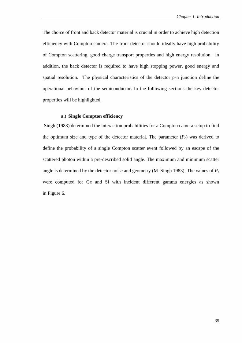
Chapter 1. Introduction
35
The choice of front and back detector material is crucial in order to achieve high detection
efficiency with Compton camera. The front detector should ideally have high probability
of Compton scattering, good charge transport properties and high energy resolution. In
addition, the back detector is required to have high stopping power, good energy and
spatial resolution. The physical characteristics of the detector p-n junction define the
operational behaviour of the semiconductor. In the following sections the key detector
properties will be highlighted.
a.) Single Compton efficiency
Singh (1983) determined the interaction probabilities for a Compton camera setup to find
the optimum size and type of the detector material. The parameter (Pc) was derived to
define the probability of a single Compton scatter event followed by an escape of the
scattered photon within a pre-described solid angle. The maximum and minimum scatter
angle is determined by the detector noise and geometry (M. Singh 1983). The values of Pc
were computed for Ge and Si with incident different gamma energies as shown
in Figure 6.
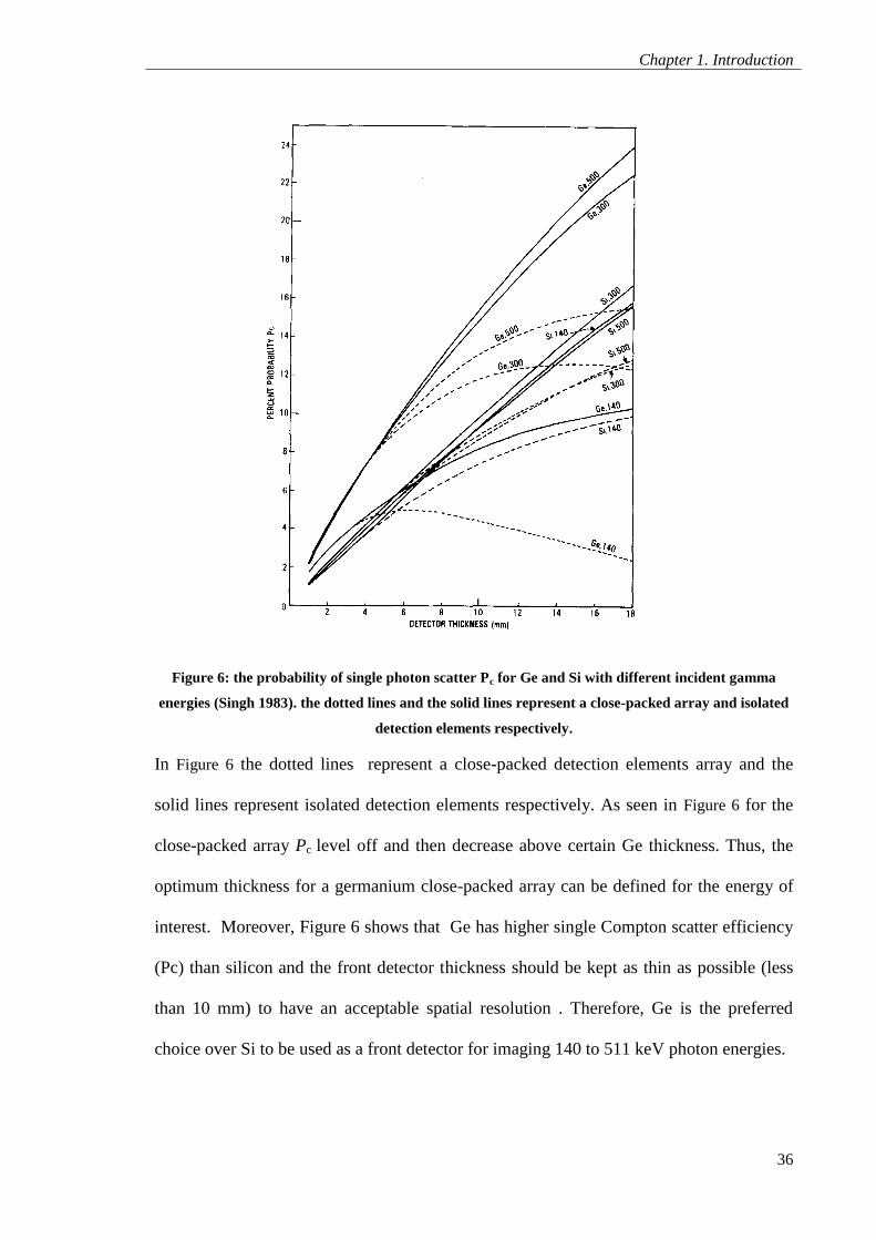
Chapter 1. Introduction
36
Figure 6: the probability of single photon scatter Pc for Ge and Si with different incident gamma
energies (Singh 1983). the dotted lines and the solid lines represent a close-packed array and isolated
detection elements respectively.
In Figure 6 the dotted lines represent a close-packed detection elements array and the
solid lines represent isolated detection elements respectively. As seen in Figure 6 for the
close-packed array Pc level off and then decrease above certain Ge thickness. Thus, the
optimum thickness for a germanium close-packed array can be defined for the energy of
interest. Moreover, Figure 6 shows that Ge has higher single Compton scatter efficiency
(Pc) than silicon and the front detector thickness should be kept as thin as possible (less
than 10 mm) to have an acceptable spatial resolution . Therefore, Ge is the preferred
choice over Si to be used as a front detector for imaging 140 to 511 keV photon energies.

Chapter 1. Introduction
37
b.) Band gap and Ionisation energy
The band-gap is the energy difference between the top of the valence band and the bottom
of the conduction band in the material (G F Knoll. 1999). The smaller the bandgap the
lower the ionisation energy required to excite an electron-hole pair, thus leading to a
better energy resolution. This is due to the fact that with smaller ionisation energy more
charge carriers are produced per unit deposited energy, hence decreasing the statistical
fluctuation.
c.) Leakage current
To achieve an efficient collection of charge carriers from any semiconductor a voltage is
applied across the active volume to create an electric field. All detectors will show a
limited conductivity (a steady-state current) even in the absence of ionizing radiation
which is called a leakage current (G F Knoll 1999). Random fluctuations in the leakage
current will obscure any small signal current following an ionizing event and this
represents a significant source of noise and thus affecting the energy resolution and
system efficiency.
Thermal generation of electron-hole pairs within the depletion region is a source of
leakage current which can be reduced by cooling the detector. Some detectors have a low
thermally generated current like silicon and can be operated at room temperature, but
germanium detectors must always operate at reduced temperature due to their low
bandgap energy as shown in Table 3 in page39. Therefore, monitoring the change in the
leakage current is important and any change or increase indicates a change in detector
efficiency that will effect the energy resolution.
d.) Charge collection properties
The preamplifier represents an interface between the detector and the signal processing
electronics. The charge carried by an incoming pulse is integrated on a capacitor and then
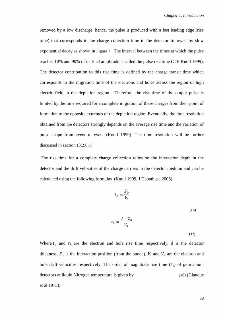
Chapter 1. Introduction
38
removed by a low discharge, hence, the pulse is produced with a fast leading edge (rise
time) that corresponds to the charge collection time in the detector followed by slow
exponential decay as shown in Figure 7 . The interval between the times at which the pulse
reaches 10% and 90% of its final amplitude is called the pulse rise time (G F Knoll 1999).
The detector contribution to this rise time is defined by the charge transit time which
corresponds to the migration time of the electrons and holes across the region of high
electric field in the depletion region. Therefore, the rise time of the output pulse is
limited by the time required for a complete migration of these charges from their point of
formation to the opposite extremes of the depletion region. Eventually, the time resolution
obtained from Ge detectors strongly depends on the average rise time and the variation of
pulse shape from event to event (Knoll 1999). The time resolution will be further
discussed in section ( 3.2.6.1).
The rise time for a complete charge collection relies on the interaction depth in the
detector and the drift velocities of the charge carriers in the detector medium and can be
calculated using the following formulas (Knoll 1999, J Gabathuse 2006) :
(16)
(17)
Where and are the electron and hole rise time respectively, d is the detector
thickness, is the interaction position (from the anode), and are the electron and
hole drift velocities respectively. The order of magnitude rise time (Tr) of germanium
detectors at liquid Nitrogen temperature is given by (18) (Giauque
et al 1973):
Chapter 1. Introduction
39
Tr ≈ W x10-8
s
(18)
where W is the thickness of the depletion region (~ detector thickness of planar detector)
measured in millimetre (mm). For the front detector in the UCL prototype camera the
active thickness of the detector is 4 mm, thus, the theoretically expected rise time (Tr) is
40 ns. Note that the theoretical rise time calculations do not take into account the effect of
trapping and de-trapping of charge carriers on the pulse shape which leads to an increase
the observed rise time.
Figure 7: Example of a preamplifier output trace fed to an oscilloscope along with a sketch of a fast
leading edge and a slow exponantial tail.
The motion of the electrons and holes formed when the incident photon deposits energy
in a semiconductor detector constitutes a current that will continue until those carriers are
completely collected. Thus, the resulting pulse represents a measure of the energy
deposited by the photon. Table 3 shows the electron and hole mobility for different
semiconductors. Note that the Ge detector has a greater charge carrier mobility than other
Time (ns)
Am
pli
tude
(A .
U)
Rise time
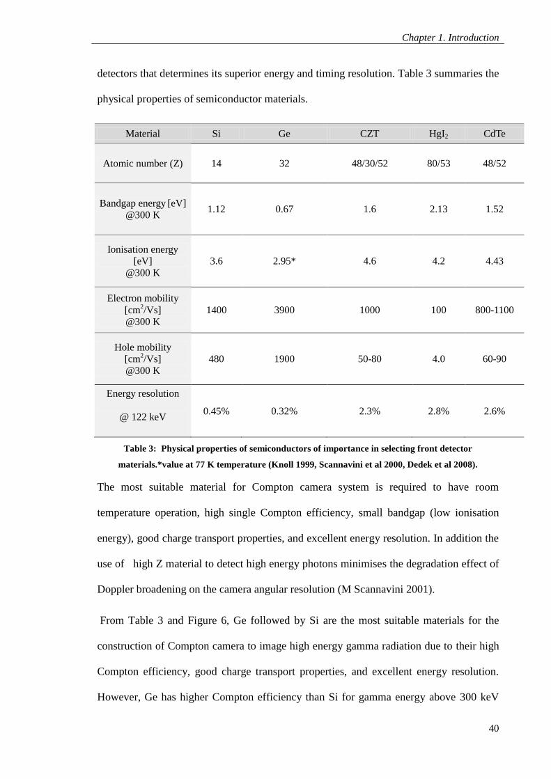
Chapter 1. Introduction
40
detectors that determines its superior energy and timing resolution. Table 3 summaries the
physical properties of semiconductor materials.
Material Si Ge CZT HgI2 CdTe
Atomic number (Z) 14 32 48/30/52 80/53 48/52
Bandgap energy [eV]
@300 K 1.12 0.67 1.6 2.13 1.52
Ionisation energy
[eV]
@300 K
3.6 2.95* 4.6 4.2 4.43
Electron mobility
[cm2/Vs]
@300 K
1400 3900 1000 100 800-1100
Hole mobility
[cm2/Vs]
@300 K
480 1900 50-80 4.0 60-90
Energy resolution
@ 122 keV 0.45%
0.32%
2.3%
2.8% 2.6%
Table 3: Physical properties of semiconductors of importance in selecting front detector
materials.*value at 77 K temperature (Knoll 1999, Scannavini et al 2000, Dedek et al 2008).
The most suitable material for Compton camera system is required to have room
temperature operation, high single Compton efficiency, small bandgap (low ionisation
energy), good charge transport properties, and excellent energy resolution. In addition the
use of high Z material to detect high energy photons minimises the degradation effect of
Doppler broadening on the camera angular resolution (M Scannavini 2001).
From Table 3 and Figure 6, Ge followed by Si are the most suitable materials for the
construction of Compton camera to image high energy gamma radiation due to their high
Compton efficiency, good charge transport properties, and excellent energy resolution.
However, Ge has higher Compton efficiency than Si for gamma energy above 300 keV
Chapter 1. Introduction
41
and the fabrication of silicon with small thickness less than 5 mm is difficult and requires
stacking of detectors, hence increasing the cost and complexity of the system. On the
other hand, fabrication of Ge detectors with up to 10mm thickness is simple (Singh 1983).
The cooling requirement for germanium detectors is a limitation and the use of cryostats
increase the camera size. The cost of germanium and silicon increases linearly with the
detector thickness.
A room temperature operated CZT detector could be used for the Compton camera, but
the low energy resolution degrades the angular resolution of the Compton camera (Dedek
et al 2008). Also, the CdTe and HgI2 room temperature operated semiconductors are not
suitable for the construction of Compton camera due to their poor energy resolution, low
Compton efficiency and poor charge collection properties as shown in Table 3. In this
thesis our studies are based upon germanium detectors as the front and back detectors as
will be explained in chapter 2. In the following section the recent and most motivating
contributions in the design and experimental development of the Compton camera for
medical applications will be reviewed.
e.) Effect of scattering materials
The absorption or scattering of the photons emitted by the source as they pass through the
object is known as the attenuation. Uncorrected attenuation results in underestimated
activity due to the reduced number of detected photons, and hence, reduces the system
sensitivity (Zaidi and Koral 2004). In emission tomography, the majority of attenuated
photons are likely to be scatter-corrupting photons. Therefore, an energy window is
usually used for the sole purpose of minimising the number of detected scattered photons.
Since Compton imaging system (similar to PET) operates at a quite large energy window
to maintain the system sensitivity, it is difficult to separate scatter primary photons (Saha
Chapter 1. Introduction
42
2010). The scatter fraction increases with increasing the energy window width. Using a
narrow energy window width is possible with the excellent germanium energy resolution
but at the expense of sensitivity (Floyd et al 1988). More details about the energy window
settings will be discussed in section 2.2.3.
The detection probability for a given event is obtained by simply multiplying the detected
photon intensity by the photons survival probability (Io/I) which is ratio of transmission
intensity before (Io) and after attenuation (I) using (19) (Rahmim and Zaidi
2008):
(19)
where µ is the attenuation along the attenuation medium of thickness x. Methods for
determining the transmission data in SPECT and PET are discussed in (section 1.4). The
interaction probabilities of incident photons with the detectors can be calculated from the
XCOM photon cross-section library available from Berger et al (1990). Reconstructing
SPECT, PET, and Compton camera images without attenuation correction can result in
reducing the count density and introduces image artefacts (Zaidi and B Hasegawa 2003).
Therefore, applying attenuation correction for Compton camera data similar to those used
in SPECT which is described in Zaidi and Hasegawa (2003) to compensate for the
attenuation effect is required for accurate quantitative measurement.
Chapter 1. Introduction
43
1.7.3 Development of Compton camera for medical imaging
The first experimental prototype of a Compton camera for medical use was designed in
the early eighties by Singh (1983). Since then, the rapid advance in the detector
technology has increased the interest in the development of the Compton camera for
medical imaging. Many studies have been carried out to develop Compton camera
systems however the actual clinical application of the camera has not yet been fully
addressed.
The focus in recent Compton camera research is mainly on the optimisation of the
Compton camera by studying the performance of different detector materials, setup, and
geometry as well as the development of appropriate image reconstruction algorithm
(Wernick and Aarsvold 2004). More effort is needed to experimentally study the
usefulness of Compton camera for nuclear medicine applications in which it can provide
an enhanced performance compared to other imaging modalities.
In the following section the recent and most motivating contributions in the design and
experimental development of the Compton camera for medical applications will be
reviewed. These contributions will be categorised by the type of the detector material
used .i.e. semiconductors, gaseous, and scintillation detectors. The following sections
describe the most significant contributions made in the last three decades to this field.
Chapter 1. Introduction
44
1.7.3.1 Semiconductors
a) Ge detectors
In 1983, Singh replaced the gamma camera mechanical collimator with a single 6x6 mm
germanium (Ge) element which served as the front (scatter) detector of Compton camera
using the NaI crystals of the gamma camera as the back (absorption) detector. Images of
Tc99m
(140 keV) and Cs137
(662 keV) sources were obtained with spatial resolution of
approximately 7 and 5 mm respectively. The sensitivity of the experiment was lower than
theoretically expected sensitivity due to the presence of dead layers on the surface of the
germanium detector used for the measurement, the low absorption efficiency of the NaI
crystal with high photon energy and the effect of Doppler broadening with low photon
energy. The camera design was improved in 1985 by using a 4x4 high purity germanium
detector array which was segmented into 16 independent 5x5x6 mm elements. Each
element was interfaced with its own circuitry to achieve better position capability. After
that in 1990, three-dimensional images of a cylindrical phantom filled with Tc99m
were
acquired and compared to gamma camera SPECT data acquired with the same phantom
(Manbir Singh & R. R. Brechner 1990). The spatial resolution of the images obtained
with electronic collimation showed no improvement compared to SPECT images mainly
due to the design and detector arrangement. The pioneer work presented by Singh in the
concept of the Compton camera medical imaging forms the basic theory and inspiration
behind all current camera developments work.
At Liverpool University, a position sensitive high purity germanium HPGe Compton
camera system was developed and evaluated (Cooper et al 2007, Boston et al 2007). Their
system was named (SmartPET) as it was meant initially to be used for small animals
imaging. The total active volume of the detector is 60 x 60 x 20 mm. The minimum
detectable gamma energy is 244 keV due to the thickness of the front detector (20 mm).
Chapter 1. Introduction
45
The spatial resolution achieved for 511 keV and 1408 keV emitting sources placed at 5
cm is 7.7 and 6.3 mm respectively. The spatial resolution of the system at 511 keV is
lower than PET as shown in Table 2. An improvement in the spatial resolution by a factor
of 2 has is expected by implementing a pulse shape analysis (PSA) technique (Cooper et
al 2007). However, the limitation of the current design and geometry necessities the need
to optimize the system to improve the imaging performance and provide a competitive
gamma ray detection system to current small animal PET. The reported camera efficiency
is 4x10⁻²
at 662 keV (Harkness et al 2009).
Recently, a hybrid Compton camera and coded mask system was developed and evaluated
for radioisotope (RI) labelled molecular probes (Takeda et al 2010). PET allows the
tracking of only one RI-labelled probe, however, their hybrid system is able to image and
track multiple probes, hence, providing better diagnosis. The spatial resolution achieved
at 3.5 cm from the camera for 834 keV emitting gamma source is 3.2 mm. However, the
efficiency of the Compton camera decreases with the thickness of the mask, thus,
optimisation of the mask thickness is needed to enhance the spatial resolution while
preserving the efficiency. Also, it is difficult to precisely calibrate the interaction position
in the encoded image detector and hence, the position resolution of the front detector
needs to improve to be 1 mm. The task of image reconstruction is more complex in the
hybrid system.
At UCL university, a pixellated Ge Compton camera was developed to image high energy
(>300 keV) gamma ray emissions in nuclear medicine examinations (G J Royle et al
2003). The system design and geometry is explained in detail in chapter 2 and the
imaging performance is discussed in chapter 3.
Chapter 1. Introduction
46
b) Si detectors
Many other researchers used Silicon (Si) as front detectors for its room temperature
operation, low cost, wide availability. An interesting study for the feasibility of Compton
camera imaging (Compton cameraI) to reconstruct the dose delivered to the patient during
radiotherapy was carried out by (Mundy and Herman 2010). An analytical model used Si
and Ge double sided strip detectors in planar configuration to study the spatial and
dosimetric resolution. The results showed that Compton cameraI is capable of
reconstructing dose distribution with a 5mm spatial resolution and 5% dose resolution.
Many technical challenges need to be addressed before implementing such a system
clinically. For instance, with the high photon energies used in radiotherapy the probability
of photon interaction with the back absorbing detector is very low .i.e. most photons will
be transmitted without interaction or may be scattered outside the detector volume. Thus,
large detector or multilayer detectors are needed. Another challenge is the image
reconstruction because many photons will be incident on the detector per second (about
4x10⁵ photons per second), and it takes 1.5 s to back project the cone associated with one
events on a 3.0 GHz processor. At this rate it will take one week to reconstruct one
backprojection image. Thus, a fast reliable reconstruction algorithm is needed for this
application.
Watanabe et al (2005) developed a Compton camera that consisted of six layered double-
sided Si Strip detectors and CdTe pixel detectors. The energy resolution was 9.1 keV
(2.5%) and 14 keV (2.7%) at 356 keV and 511 keV, respectively. Improvements in CdTe
detectors to achieve better energy resolution are needed. Images for different radioisotope
energies (122 to 662 keV) were obtained and reconstructed using a backprojection
algorithm. The images were distorted by the backprojection artefacts due to the
asymmetric arrangement of the CdTe absorbers used. Thus, having a symmetric CdTe
Chapter 1. Introduction
47
absorbers arrangement is required. The angular resolution was 3.9° (FWHM) for 511 keV
gamma-ray photons.
At Michigan University, a prototype Compton camera (C-SPRINT) designed with a
single pad Si detector surrounded by a SPRINT scintillation ring intended for low energy
gamma-ray imaging for nuclear medicine applications was developed by Leblanc et al
(1998). The SPRINT scintillation ring is a SPECT imaging system made up of eleven
modules arranged in a 50 cm diameter ring shape with its lead collimators removed.
Employing ring geometry improved spatial resolution and reduce single count rates in the
second detector. Simulations results show angular uncertainties of 4.1° and 2.2° FWHM
for Tc99m
and I131
point sources, respectively. The results showed that the C-SPRINT
sensitivity is 2.7 x10⁻³
at 140 keV which is lower than the mechanically-collimated
gamma camera. Thus, it is necessary to improve the design by stacking arrays of silicon
pad detectors in conjunction with an optimized second detector cylinder with a ring radius
reduced to 12.5 cm. The C-SPRINT system had approximately equal performance for I131
compared to gamma camera, and could exceed the sensitivity with an optimized design.
The overall position uncertainty for an I131
point source at 10 cm was 4.1 mm.
Ten years later, Han et al (2008) compared theoretically the imaging performance of a
planar Si (scatter detector) and NaI (absorption detector) Compton camera with a HEGP
collimator gamma camera using a statistical model. A cylindrical hot spot disk with 0.6
cm, 0.8 cm, 1.0 cm, 1.5 cm, 2.0 cm and 2.4 cm diameter spots was simulated with I131
emitted photons. The results show that if the same number of events is used the imaging
performance of the Compton system is better than the gamma camera for hot spots width
below∼1.1 cm, this advantage decrease for spot size above 1.1 cm. The result shows that
the effect of Doppler broadening is the limiting factor for Compton camera performance
for imaging 364.4 keV photons. Also, the results show that the detection sensitivity of the
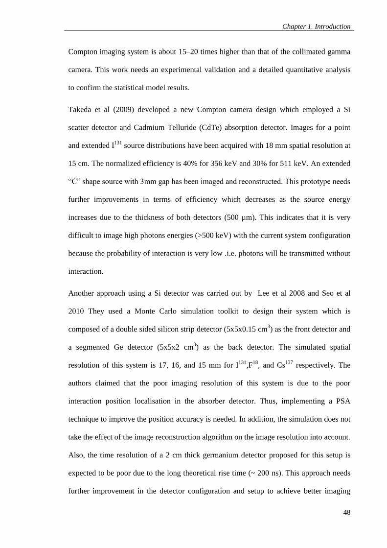
Chapter 1. Introduction
48
Compton imaging system is about 15–20 times higher than that of the collimated gamma
camera. This work needs an experimental validation and a detailed quantitative analysis
to confirm the statistical model results.
Takeda et al (2009) developed a new Compton camera design which employed a Si
scatter detector and Cadmium Telluride (CdTe) absorption detector. Images for a point
and extended I131
source distributions have been acquired with 18 mm spatial resolution at
15 cm. The normalized efficiency is 40% for 356 keV and 30% for 511 keV. An extended
“C” shape source with 3mm gap has been imaged and reconstructed. This prototype needs
further improvements in terms of efficiency which decreases as the source energy
increases due to the thickness of both detectors (500 µm). This indicates that it is very
difficult to image high photons energies (>500 keV) with the current system configuration
because the probability of interaction is very low .i.e. photons will be transmitted without
interaction.
Another approach using a Si detector was carried out by Lee et al 2008 and Seo et al
2010 They used a Monte Carlo simulation toolkit to design their system which is
composed of a double sided silicon strip detector (5x5x0.15 cm3) as the front detector and
a segmented Ge detector (5x5x2 cm3) as the back detector. The simulated spatial
resolution of this system is 17, 16, and 15 mm for I131
,F18
, and Cs137
respectively. The
authors claimed that the poor imaging resolution of this system is due to the poor
interaction position localisation in the absorber detector. Thus, implementing a PSA
technique to improve the position accuracy is needed. In addition, the simulation does not
take the effect of the image reconstruction algorithm on the image resolution into account.
Also, the time resolution of a 2 cm thick germanium detector proposed for this setup is
expected to be poor due to the long theoretical rise time (~ 200 ns). This approach needs
further improvement in the detector configuration and setup to achieve better imaging
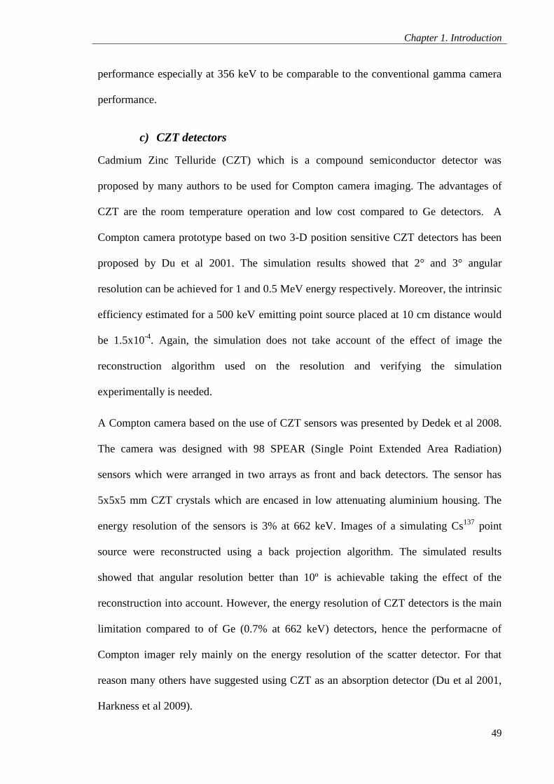
Chapter 1. Introduction
49
performance especially at 356 keV to be comparable to the conventional gamma camera
performance.
c) CZT detectors
Cadmium Zinc Telluride (CZT) which is a compound semiconductor detector was
proposed by many authors to be used for Compton camera imaging. The advantages of
CZT are the room temperature operation and low cost compared to Ge detectors. A
Compton camera prototype based on two 3-D position sensitive CZT detectors has been
proposed by Du et al 2001. The simulation results showed that 2° and 3° angular
resolution can be achieved for 1 and 0.5 MeV energy respectively. Moreover, the intrinsic
efficiency estimated for a 500 keV emitting point source placed at 10 cm distance would
be 1.5x10⁻⁴
. Again, the simulation does not take account of the effect of image the
reconstruction algorithm used on the resolution and verifying the simulation
experimentally is needed.
A Compton camera based on the use of CZT sensors was presented by Dedek et al 2008.
The camera was designed with 98 SPEAR (Single Point Extended Area Radiation)
sensors which were arranged in two arrays as front and back detectors. The sensor has
5x5x5 mm CZT crystals which are encased in low attenuating aluminium housing. The
energy resolution of the sensors is 3% at 662 keV. Images of a simulating Cs137
point
source were reconstructed using a back projection algorithm. The simulated results
showed that angular resolution better than 10º is achievable taking the effect of the
reconstruction into account. However, the energy resolution of CZT detectors is the main
limitation compared to of Ge (0.7% at 662 keV) detectors, hence the performacne of
Compton imager rely mainly on the energy resolution of the scatter detector. For that
reason many others have suggested using CZT as an absorption detector (Du et al 2001,
Harkness et al 2009).
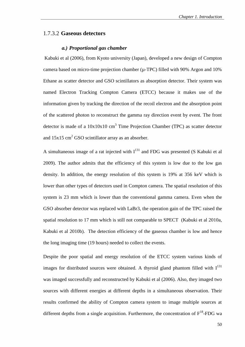
Chapter 1. Introduction
50
1.7.3.2 Gaseous detectors
a.) Proportional gas chamber
Kabuki et al (2006), from Kyoto university (Japan), developed a new design of Compton
camera based on micro-time projection chamber (µ-TPC) filled with 90% Argon and 10%
Ethane as scatter detector and GSO scintillators as absorption detector. Their system was
named Electron Tracking Compton Camera (ETCC) because it makes use of the
information given by tracking the direction of the recoil electron and the absorption point
of the scattered photon to reconstruct the gamma ray direction event by event. The front
detector is made of a 10x10x10 cm3 Time Projection Chamber (TPC) as scatter detector
and 15x15 cm2 GSO scintillator array as an absorber.
A simultaneous image of a rat injected with I131
and FDG was presented (S Kabuki et al
2009). The author admits that the efficiency of this system is low due to the low gas
density. In addition, the energy resolution of this system is 19% at 356 keV which is
lower than other types of detectors used in Compton camera. The spatial resolution of this
system is 23 mm which is lower than the conventional gamma camera. Even when the
GSO absorber detector was replaced with LaBr3, the operation gain of the TPC raised the
spatial resolution to 17 mm which is still not comparable to SPECT (Kabuki et al 2010a,
Kabuki et al 2010b). The detection efficiency of the gaseous chamber is low and hence
the long imaging time (19 hours) needed to collect the events.
Despite the poor spatial and energy resolution of the ETCC system various kinds of
images for distributed sources were obtained. A thyroid gland phantom filled with I131
was imaged successfully and reconstructed by Kabuki et al (2006). Also, they imaged two
sources with different energies at different depths in a simultaneous observation. Their
results confirmed the ability of Compton camera system to image multiple sources at
different depths from a single acquisition. Furthermore, the concentration of F18
-FDG wa
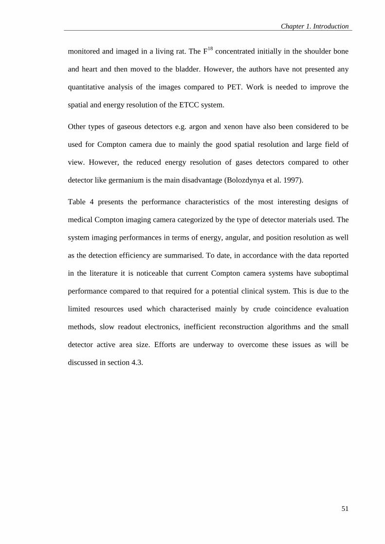
Chapter 1. Introduction
51
monitored and imaged in a living rat. The F18
concentrated initially in the shoulder bone
and heart and then moved to the bladder. However, the authors have not presented any
quantitative analysis of the images compared to PET. Work is needed to improve the
spatial and energy resolution of the ETCC system.
Other types of gaseous detectors e.g. argon and xenon have also been considered to be
used for Compton camera due to mainly the good spatial resolution and large field of
view. However, the reduced energy resolution of gases detectors compared to other
detector like germanium is the main disadvantage (Bolozdynya et al. 1997).
Table 4 presents the performance characteristics of the most interesting designs of
medical Compton imaging camera categorized by the type of detector materials used. The
system imaging performances in terms of energy, angular, and position resolution as well
as the detection efficiency are summarised. To date, in accordance with the data reported
in the literature it is noticeable that current Compton camera systems have suboptimal
performance compared to that required for a potential clinical system. This is due to the
limited resources used which characterised mainly by crude coincidence evaluation
methods, slow readout electronics, inefficient reconstruction algorithms and the small
detector active area size. Efforts are underway to overcome these issues as will be
discussed in section 4.3.
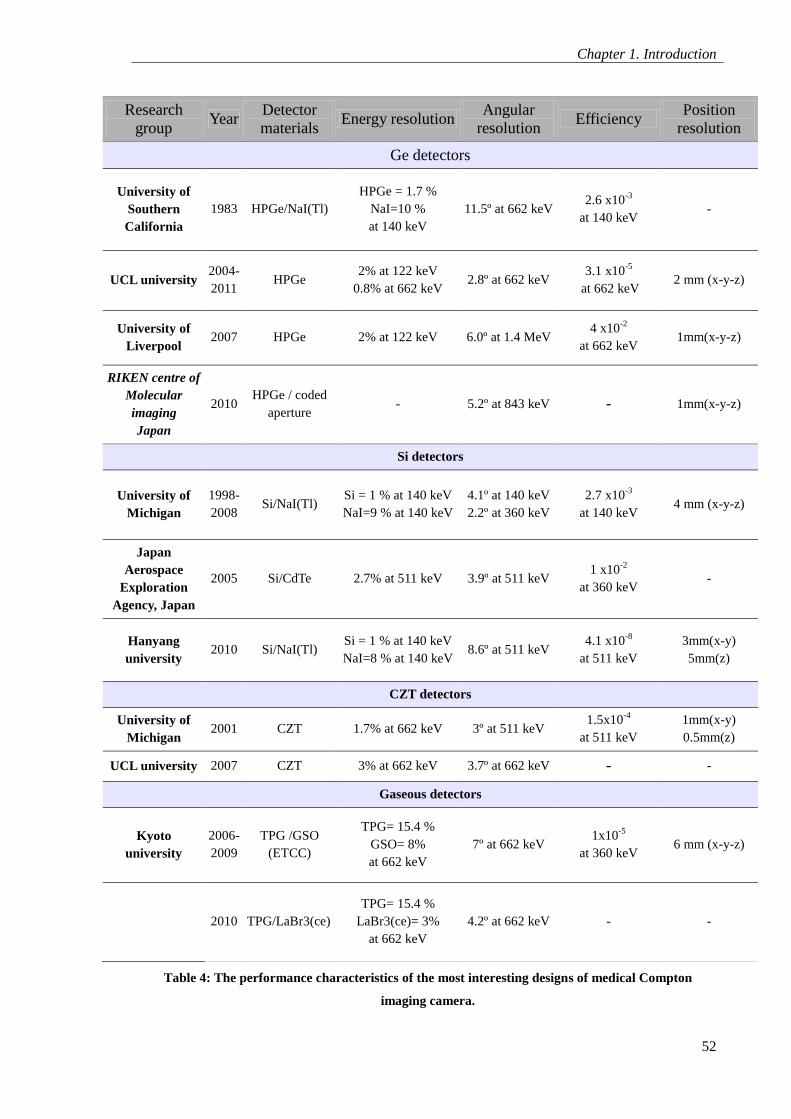
Chapter 1. Introduction
52
Research
group Year
Detector
materials Energy resolution
Angular
resolution Efficiency
Position
resolution
Ge detectors
University of
Southern
California
1983 HPGe/NaI(Tl)
HPGe = 1.7 %
NaI=10 %
at 140 keV
11.5º at 662 keV 2.6 x10
-3
at 140 keV -
UCL university 2004-
2011 HPGe
2% at 122 keV
0.8% at 662 keV 2.8º at 662 keV
3.1 x10⁻⁵
at 662 keV 2 mm (x-y-z)
University of
Liverpool 2007 HPGe 2% at 122 keV 6.0º at 1.4 MeV
4 x10⁻²
at 662 keV 1mm(x-y-z)
RIKEN centre of
Molecular
imaging
Japan
2010 HPGe / coded
aperture - 5.2º at 843 keV - 1mm(x-y-z)
Si detectors
University of
Michigan
1998-
2008 Si/NaI(Tl)
Si = 1 % at 140 keV
NaI=9 % at 140 keV
4.1º at 140 keV
2.2º at 360 keV
2.7 x10⁻³
at 140 keV 4 mm (x-y-z)
Japan
Aerospace
Exploration
Agency, Japan
2005 Si/CdTe 2.7% at 511 keV 3.9º at 511 keV 1 x10
-2
at 360 keV -
Hanyang
university 2010 Si/NaI(Tl)
Si = 1 % at 140 keV
NaI=8 % at 140 keV 8.6º at 511 keV
4.1 x10⁻⁸
at 511 keV
3mm(x-y)
5mm(z)
CZT detectors
University of
Michigan 2001 CZT 1.7% at 662 keV 3º at 511 keV
1.5x10⁻⁴
at 511 keV
1mm(x-y)
0.5mm(z)
UCL university 2007 CZT 3% at 662 keV 3.7º at 662 keV - -
Gaseous detectors
Kyoto
university
2006-
2009
TPG /GSO
(ETCC)
TPG= 15.4 %
GSO= 8%
at 662 keV
7º at 662 keV 1x10
-5
at 360 keV 6 mm (x-y-z)
2010 TPG/LaBr3(ce)
TPG= 15.4 %
LaBr3(ce)= 3%
at 662 keV
4.2º at 662 keV - -
Table 4: The performance characteristics of the most interesting designs of medical Compton
imaging camera.
Chapter 1. Introduction
53
1.8 Structure of Thesis
The following information is divided into three chapters: materials and methods, results
and discussions, and conclusions and future works. The materials and methods chapter
describes the UCL Compton camera design and the associated controlling readout
electronics as well as the operational mode, data filtering, and image reconstruction
principles
The results and discussions chapter describes the physical and imaging performance of
the camera followed by a detailed quantitative analysis of the results. Moreover, the
images obtained with the Compton camera are compared to other systems used in nuclear
medicine (gamma camera and PET).
Finally, the conclusions and further work chapter will indicate the theoretical and
practical implication of the work presented in this thesis and the contribution that this
work presents to the field along with the limitations of this work and how can it be
overcome and optimized with future research.
1.9 Novel Work Undertaken
A Multiple views technique was used to image the source from different angles
and simulate the pixel arrangement in the full camera.
A Cylindrical Perspex phantom was designed and imaged with F18
and I131
for the
first time with the UCL Compton camera.
The UCL Compton camera phantom images were compared to gamma camera
and PET images quantitatively for the first time.
Chapter 2: Materials and Methods
54
Chapter 2
2 Materials and Methods
2.1 Camera geometrical design description
The camera is a prototype for medical application built at the ORTEC detector R&D plant
at Oak Ridge Tennessee, and it consists of two planes of pixilated HPGe detectors in the
same vacuum housing. The front (scatter) detector pixels are clustered in 8 arrays
distributed around a ring. The front detector is a solid disc of germanium which has a
diameter of 100 mm and a thickness of 4 mm, but only the outer region is active. The
total number of pixels in the front detector is 152.
The back (absorption) detector consists of one 5 x 5 pixel group and has a diameter of
28 mm and thickness of 10 mm. The pixels are 4x4 mm2 and are spaced by 1 mm. The
front and back detector are separated by 9.7 cm as shown in Figure 8. The pixellated outer
ring has a 10 cm width. The front detector plane is positioned towards the front of the
outer surface of the cryostat as shown in Figure 8. A circular indentation has been made in
the end cap to position a lead disc to shield the back detector from direct interaction as
will be discussed in section 3.1.2.
Germanium detectors cannot operate at room temperature due to the small bandgap and
the large thermally induced leakage current that would result. The camera is cooled to
about 200°C (77° K) by liquid Nitrogen to reduce the leakage current noise and prevent it
from spoiling the excellent energy resolution of germanium (G F Knoll. 1999). The liquid
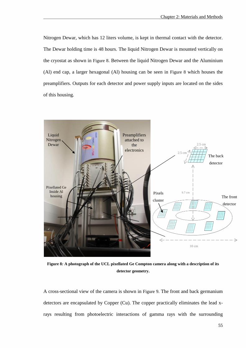
Chapter 2: Materials and Methods
55
Nitrogen Dewar, which has 12 liters volume, is kept in thermal contact with the detector.
The Dewar holding time is 48 hours. The liquid Nitrogen Dewar is mounted vertically on
the cryostat as shown in Figure 8. Between the liquid Nitrogen Dewar and the Aluminium
(Al) end cap, a larger hexagonal (Al) housing can be seen in Figure 8 which houses the
preamplifiers. Outputs for each detector and power supply inputs are located on the sides
of this housing.
Figure 8: A photograph of the UCL pixellated Ge Compton camera along with a description of its
detector geometry.
A cross-sectional view of the camera is shown in Figure 9. The front and back germanium
detectors are encapsulated by Copper (Cu). The copper practically eliminates the lead x-
rays resulting from photoelectric interactions of gamma rays with the surrounding
The front
detector
9.7 cm
The back
detector
Liquid
Nitrogen
Dewar
Pixellated Ge
Inside Al
housing
Preamplifiers
attached to
the
electronics 2.5 cm
2.5 cm
10 cm
Pixels
cluster
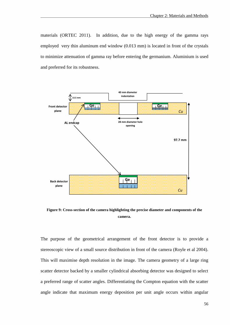
Chapter 2: Materials and Methods
56
materials (ORTEC 2011). In addition, due to the high energy of the gamma rays
employed very thin aluminum end window (0.013 mm) is located in front of the crystals
to minimize attenuation of gamma ray before entering the germanium. Aluminium is used
and preferred for its robustness.
Copper Ge
Ge Ge
AL endcap
97.7 mm
13.5 mm
28 mm diameter hole
opening
40 mm diameter
indentation
Front detector
plane
Back detector
plane
Ge
Ge Ge
Cu
Cu
Figure 9: Cross-section of the camera highlighting the precise diameter and components of the
camera.
The purpose of the geometrical arrangement of the front detector is to provide a
stereoscopic view of a small source distribution in front of the camera (Royle et al 2004).
This will maximise depth resolution in the image. The camera geometry of a large ring
scatter detector backed by a smaller cylindrical absorbing detector was designed to select
a preferred range of scatter angles. Differentiating the Compton equation with the scatter
angle indicate that maximum energy deposition per unit angle occurs within angular
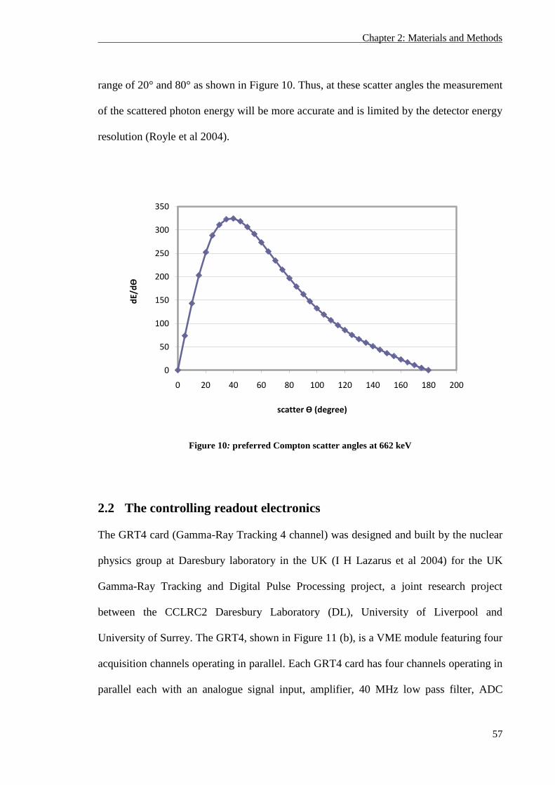
Chapter 2: Materials and Methods
57
range of 20° and 80° as shown in Figure 10. Thus, at these scatter angles the measurement
of the scattered photon energy will be more accurate and is limited by the detector energy
resolution (Royle et al 2004).
Figure 10: preferred Compton scatter angles at 662 keV
2.2 The controlling readout electronics
The GRT4 card (Gamma-Ray Tracking 4 channel) was designed and built by the nuclear
physics group at Daresbury laboratory in the UK (I H Lazarus et al 2004) for the UK
Gamma-Ray Tracking and Digital Pulse Processing project, a joint research project
between the CCLRC2 Daresbury Laboratory (DL), University of Liverpool and
University of Surrey. The GRT4, shown in Figure 11 (b), is a VME module featuring four
acquisition channels operating in parallel. Each GRT4 card has four channels operating in
parallel each with an analogue signal input, amplifier, 40 MHz low pass filter, ADC
0
50
100
150
200
250
300
350
0 20 40 60 80 100 120 140 160 180 200
dE/
dѲ
scatter Ѳ (degree)
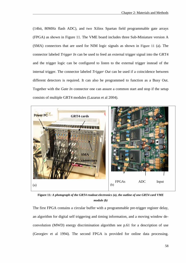
Chapter 2: Materials and Methods
58
(14bit, 80MHz flash ADC), and two Xilinx Spartan field programmable gate arrays
(FPGA) as shown in Figure 11. The VME board includes three Sub-Miniature version A
(SMA) connectors that are used for NIM logic signals as shown in Figure 11 (a). The
connector labeled Trigger In can be used to feed an external trigger signal into the GRT4
and the trigger logic can be configured to listen to the external trigger instead of the
internal trigger. The connector labeled Trigger Out can be used if a coincidence between
different detectors is required. It can also be programmed to function as a Busy Out.
Together with the Gate In connector one can assure a common start and stop if the setup
consists of multiple GRT4 modules (Lazarus et al 2004).
(a)
(b)
Figure 11: A photograph of the GRT4 readout electronics (a), the outline of one GRT4 card VME
module (b)
The first FPGA contains a circular buffer with a programmable pre-trigger register delay,
an algorithm for digital self triggering and timing information, and a moving window de-
convolution (MWD) energy discrimination algorithm see p.61 for a description of use
(Georgiev et al 1994). The second FPGA is provided for online data processing.
GRT4 cards Power PC Power PC
Input ADC FPGAs
SMA
connectors
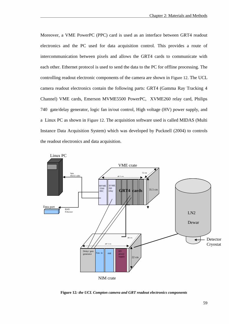
Chapter 2: Materials and Methods
59
Moreover, a VME PowerPC (PPC) card is used as an interface between GRT4 readout
electronics and the PC used for data acquisition control. This provides a route of
intercommunication between pixels and allows the GRT4 cards to communicate with
each other. Ethernet protocol is used to send the data to the PC for offline processing. The
controlling readout electronic components of the camera are shown in Figure 12. The UCL
camera readout electronics contain the following parts: GRT4 (Gamma Ray Tracking 4
Channel) VME cards, Emerson MVME5500 PowerPC, XVME260 relay card, Philips
740 gate/delay generator, logic fan in/out control, High voltage (HV) power supply, and
a Linux PC as shown in Figure 12. The acquisition software used is called MIDAS (Multi
Instance Data Acquisition System) which was developed by Pucknell (2004) to controls
the readout electronics and data acquisition.
Figure 12: the UCL Compton camera and GRT readout electronics components
52 cm
35.5 cm
48.3 cm
MVME
5500
PPC
PPC
XVME
260
relay
relay
Linux PC
Data port
9pin
RS232 cable
RJ45
Ethernet
cable
Delay/ gate
generator Fan- in
HV
power
supply
Detector
Cryostat 48.3 cm
48 cm
22 cm
VME crate
NIM crate
GRT4 cards
out
LN2
Dewar LN2
Dewar
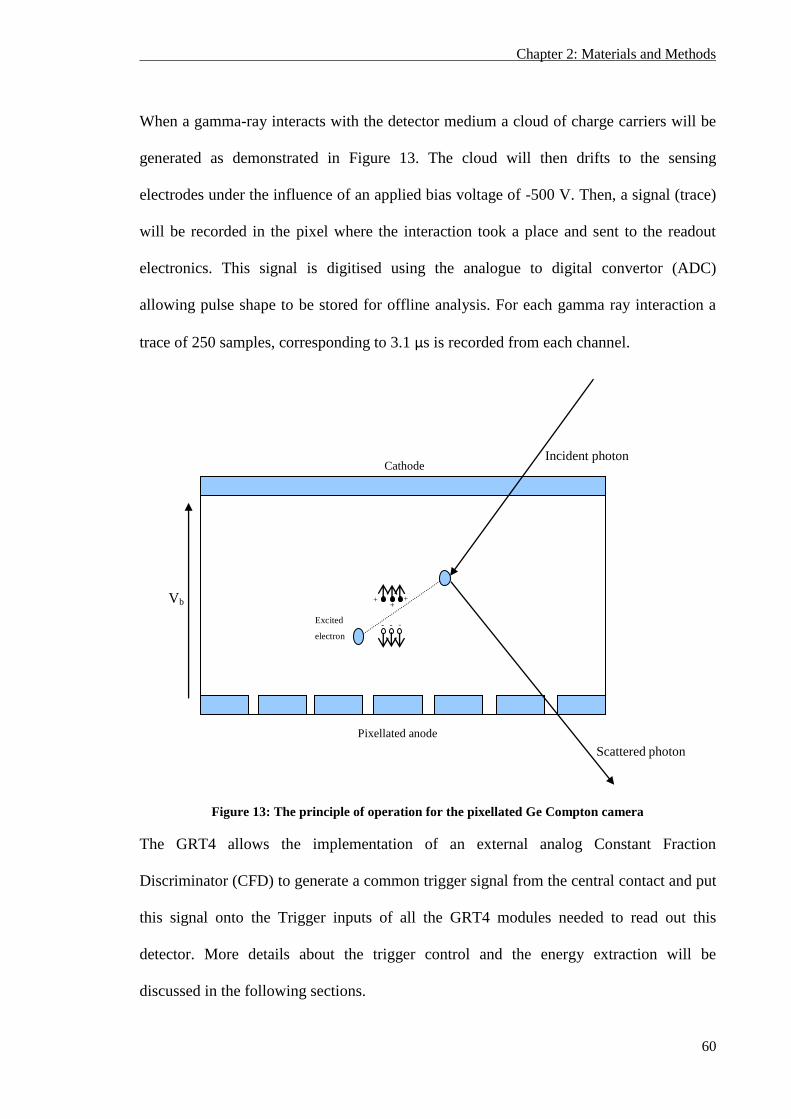
Chapter 2: Materials and Methods
60
When a gamma-ray interacts with the detector medium a cloud of charge carriers will be
generated as demonstrated in Figure 13. The cloud will then drifts to the sensing
electrodes under the influence of an applied bias voltage of -500 V. Then, a signal (trace)
will be recorded in the pixel where the interaction took a place and sent to the readout
electronics. This signal is digitised using the analogue to digital convertor (ADC)
allowing pulse shape to be stored for offline analysis. For each gamma ray interaction a
trace of 250 samples, corresponding to 3.1 µs is recorded from each channel.
Figure 13: The principle of operation for the pixellated Ge Compton camera
The GRT4 allows the implementation of an external analog Constant Fraction
Discriminator (CFD) to generate a common trigger signal from the central contact and put
this signal onto the Trigger inputs of all the GRT4 modules needed to read out this
detector. More details about the trigger control and the energy extraction will be
discussed in the following sections.
Cathode
Incident photon
Excited
electron
+ +
+
Scattered photon
- - -
Vb
Pixellated anode
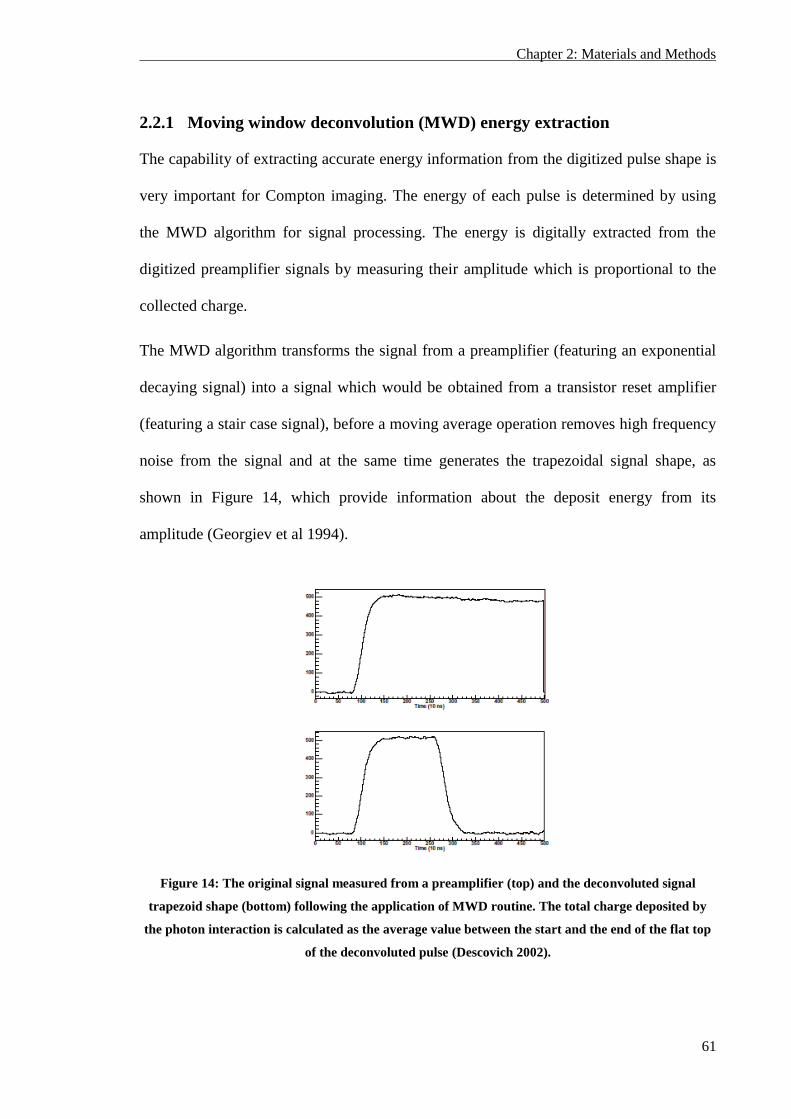
Chapter 2: Materials and Methods
61
2.2.1 Moving window deconvolution (MWD) energy extraction
The capability of extracting accurate energy information from the digitized pulse shape is
very important for Compton imaging. The energy of each pulse is determined by using
the MWD algorithm for signal processing. The energy is digitally extracted from the
digitized preamplifier signals by measuring their amplitude which is proportional to the
collected charge.
The MWD algorithm transforms the signal from a preamplifier (featuring an exponential
decaying signal) into a signal which would be obtained from a transistor reset amplifier
(featuring a stair case signal), before a moving average operation removes high frequency
noise from the signal and at the same time generates the trapezoidal signal shape, as
shown in Figure 14, which provide information about the deposit energy from its
amplitude (Georgiev et al 1994).
Figure 14: The original signal measured from a preamplifier (top) and the deconvoluted signal
trapezoid shape (bottom) following the application of MWD routine. The total charge deposited by
the photon interaction is calculated as the average value between the start and the end of the flat top
of the deconvoluted pulse (Descovich 2002).
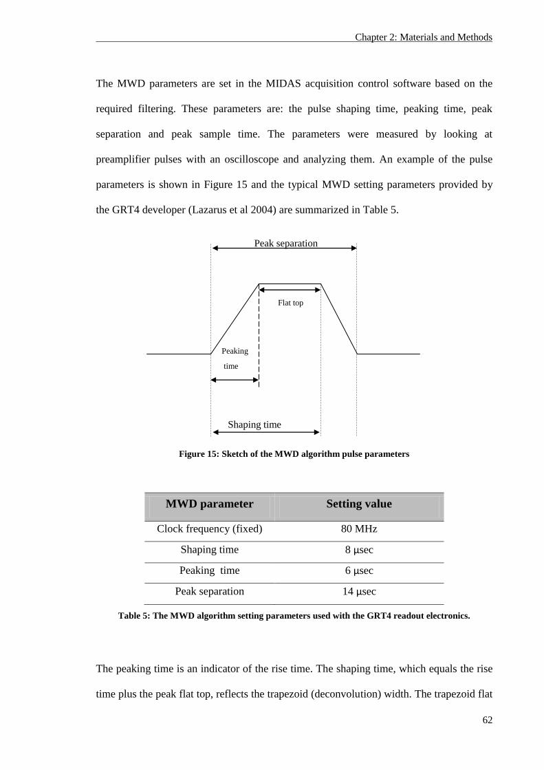
Chapter 2: Materials and Methods
62
The MWD parameters are set in the MIDAS acquisition control software based on the
required filtering. These parameters are: the pulse shaping time, peaking time, peak
separation and peak sample time. The parameters were measured by looking at
preamplifier pulses with an oscilloscope and analyzing them. An example of the pulse
parameters is shown in Figure 15 and the typical MWD setting parameters provided by
the GRT4 developer (Lazarus et al 2004) are summarized in Table 5.
Figure 15: Sketch of the MWD algorithm pulse parameters
MWD parameter Setting value
Clock frequency (fixed) 80 MHz
Shaping time 8 µsec
Peaking time 6 µsec
Peak separation 14 µsec
Table 5: The MWD algorithm setting parameters used with the GRT4 readout electronics.
The peaking time is an indicator of the rise time. The shaping time, which equals the rise
time plus the peak flat top, reflects the trapezoid (deconvolution) width. The trapezoid flat
Shaping time
Peaking
time
Peak separation
Flat top
Chapter 2: Materials and Methods
63
top value reflects the total charge (energy) deposited by the gamma-ray interaction. The
peak separation is set to the sum of the shaping and two peaking times. Further details
will be presented in section 3.2.1 about the effect of the trapezoid window width on the
energy resolution.
2.2.2 Triggering and flow control
Discriminators generate precise logic pulses in response to input signals exceeding a
given threshold. There are two key types of discriminators: the leading edge
discriminator and the constant fraction discriminator (CFD). The leading edge
discriminator produces an output pulse at the time when the input pulse crosses a given
threshold voltage. The CFD is used as an internal trigger for each GRT channel to
generate a logic pulse whose leading edge indicates the timing information for input
signals above constant fraction of the peak pulse amplitude (Knoll 1999). The digital
CFD can be described by the following formula (Crespi et al 2010):
(20)
where Sin is the input signal, S out is the output signal, ti is the sampling time (=12.5ns), F
is fixed fraction value (=0.5) and d is the shaping delay time (=50 ns). The only
programmable parameter is the CFD threshold set (discriminator level). The CFD will
trigger (produce an output pulse) only if the voltage of the input from the detector
preamplifier crosses the threshold set. The best leading edge timing characteristics are
obtained when the timing discriminator is set to about 10 to 20 % of the pulse amplitude
(Knoll 1999). A detailed investigation of the effect of the CFD discriminator level on the
reconstructed data will be described in (section 3.2.6.3).
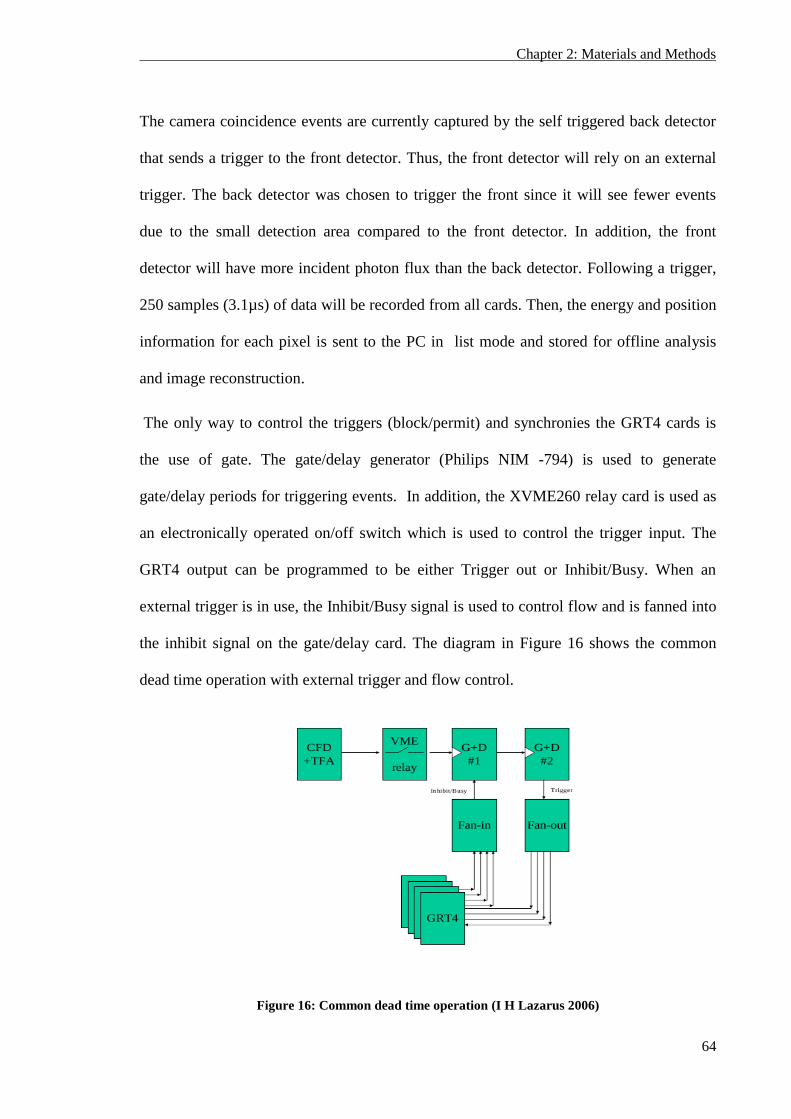
Chapter 2: Materials and Methods
64
The camera coincidence events are currently captured by the self triggered back detector
that sends a trigger to the front detector. Thus, the front detector will rely on an external
trigger. The back detector was chosen to trigger the front since it will see fewer events
due to the small detection area compared to the front detector. In addition, the front
detector will have more incident photon flux than the back detector. Following a trigger,
250 samples (3.1µs) of data will be recorded from all cards. Then, the energy and position
information for each pixel is sent to the PC in list mode and stored for offline analysis
and image reconstruction.
The only way to control the triggers (block/permit) and synchronies the GRT4 cards is
the use of gate. The gate/delay generator (Philips NIM -794) is used to generate
gate/delay periods for triggering events. In addition, the XVME260 relay card is used as
an electronically operated on/off switch which is used to control the trigger input. The
GRT4 output can be programmed to be either Trigger out or Inhibit/Busy. When an
external trigger is in use, the Inhibit/Busy signal is used to control flow and is fanned into
the inhibit signal on the gate/delay card. The diagram in Figure 16 shows the common
dead time operation with external trigger and flow control.
Figure 16: Common dead time operation (I H Lazarus 2006)
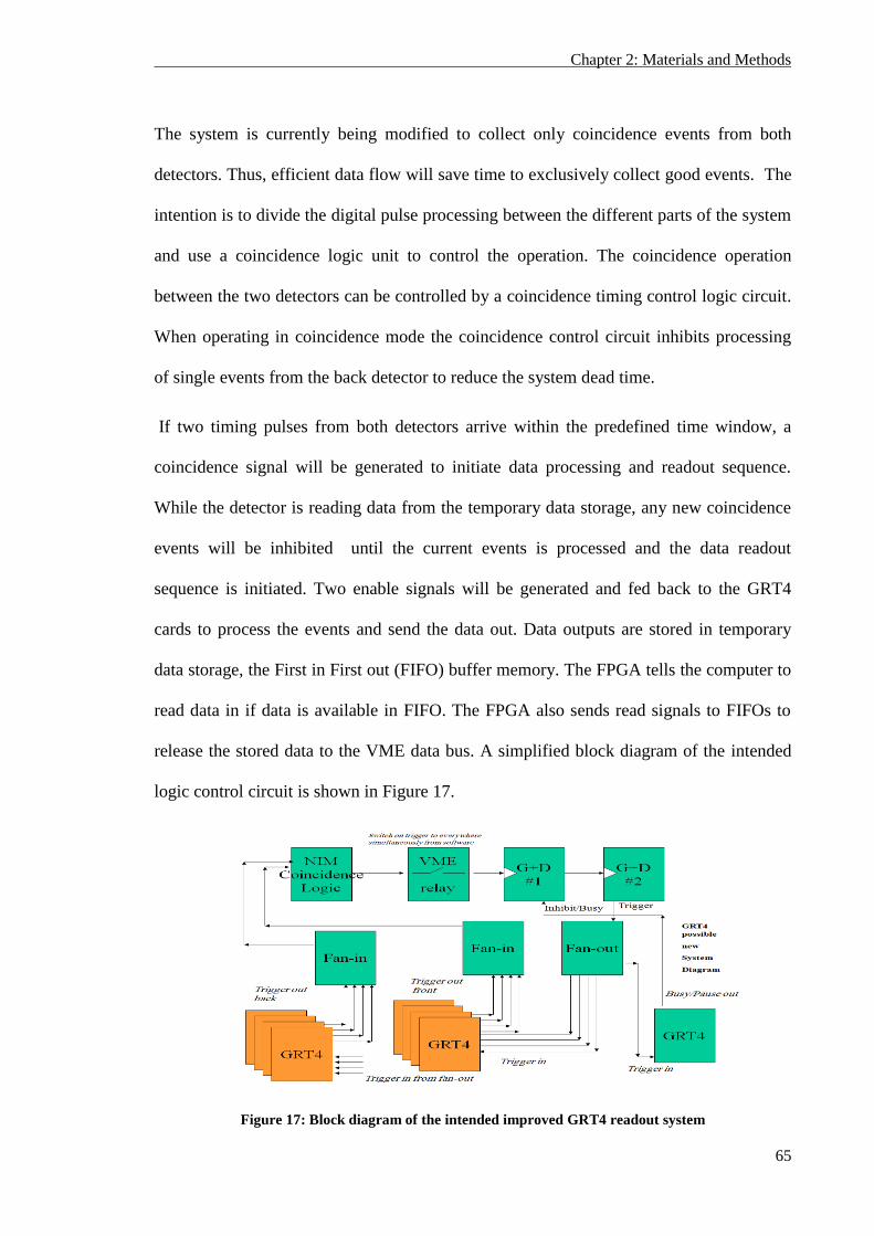
Chapter 2: Materials and Methods
65
The system is currently being modified to collect only coincidence events from both
detectors. Thus, efficient data flow will save time to exclusively collect good events. The
intention is to divide the digital pulse processing between the different parts of the system
and use a coincidence logic unit to control the operation. The coincidence operation
between the two detectors can be controlled by a coincidence timing control logic circuit.
When operating in coincidence mode the coincidence control circuit inhibits processing
of single events from the back detector to reduce the system dead time.
If two timing pulses from both detectors arrive within the predefined time window, a
coincidence signal will be generated to initiate data processing and readout sequence.
While the detector is reading data from the temporary data storage, any new coincidence
events will be inhibited until the current events is processed and the data readout
sequence is initiated. Two enable signals will be generated and fed back to the GRT4
cards to process the events and send the data out. Data outputs are stored in temporary
data storage, the First in First out (FIFO) buffer memory. The FPGA tells the computer to
read data in if data is available in FIFO. The FPGA also sends read signals to FIFOs to
release the stored data to the VME data bus. A simplified block diagram of the intended
logic control circuit is shown in Figure 17.
Figure 17: Block diagram of the intended improved GRT4 readout system
Chapter 2: Materials and Methods
66
2.2.3 Data filtering
Currently, the camera operates in an offline data analysis mode i.e. all events will be
collected from the camera and then only coincident event will be selected offline for
image reconstruction. About 1 TB of data is usually collected for each image. Then an
offline data filtering code is used, which is written in Interactive Data Language (IDL), to
filter the data and chose only events interacting with front and back detectors within a
predefined time and energy window. This reduces the data set by about 80% resulting in a
4 GB data size.
For each interaction the GRT4 electronics channel number, MWD energy, and a
timestamp were all recorded in the raw data file. The data filtering code works by first
removing single events which only occurs in the back detector without being scattered in
the front detector. Then, the code select only coincident (useful) events that falls within
75 ns time window (more details about the time window selection will be discussed in
section 3.2.6) and fulfilling the energy window condition; which is described by
(21):
| Ef +Eb – Esource |< energy window
(21)
where Ef and Eb are the measured front and back detector energy respectively. For
instance, if the energy window is set to 350 keV only events deposit total energy minus
the source energy smaller than 350 keV (i.e. the total deposited energy should be less than
or equal to 313 keV) will be selected as useful event. The electronics channel numbers in
which the interaction was recorded will be converted into physical positions in space
(pixel positions) and the energy will be extracted from measuring the height of the signal
by MWD algorithm. The data is then stored in a data file which will be created for the
Chapter 2: Materials and Methods
67
image reconstruction algorithm including the x, y, z, and the energy (Emwd) for pixels in
which the coincidence event was detected. This data file is then used as an input for the
image reconstruction code which is written in C++ language.
2.3 Image reconstruction
The backprojection is the most common straightforward algorithm used in the
reconstruction of the cross-sectional images data obtained from many imaging modalities
(R J Ott 1986). A simple backprojection algorithm is used for straightforward image
reconstruction for the data obtained from Compton camera simply by superposition of all
conical surfaces resulting from each interaction (Wilderman et al 1998). Using a 3GHz
Pentium processor the time taken to reconstruct 100x100 pixels image with 20000 events
is 6 seconds. Back projection is a very useful reconstruction method that provides an easy
to interpret image as well as providing a starting point for some iterative image
reconstruction methods.
To reconstruct a 2D image a specific image plane should first be chosen. Then, the
intersection of the cones with the image plane is then determined which can be an ellipse,
a parabola or a hyperbola depending on the angle between the cone axis and the plane.
Thus, the intensity of every image pixel is given by the number of conic sections crossing
the pixel. The superposition of all conic sections is simply the back projection image
(Wilderman et al 1998). The backprojection image of a point source is also called point
spread function that describes the response of the imaging system. Image reconstruction is
particularly challenging for Compton camera because the point spread function is not
constant and varies with source position (Wilderman et al 1998, Dedek et al 2009).
Chapter 2: Materials and Methods
68
For 3D image reconstruction this procedure is repeated for several image planes as
shown in Figure 4. The main problem of backprojection reconstruction for Compton
camera images is the introduction of image artifacts that leads to degradation in the image
resolution (Martin et al 1994) as will be demonstrated in the results chapter.
Although list mode backprojection reconstruction is simple and fast, in Compton scatter
imaging the intersection of the backprojected ellipses and the source plane results in
image error or artifacts. These artifacts can be defined as the extra unwanted information
that is artificially produced by the reconstruction algorithm that the original imaged object
did not contain (Ahmed 2007). Iterative algorithms like MLEM (Maximum Likelihood
Expectation Maximization) or order subset expectation maximization (OSEM) could be
used to overcome these problems and result in a better estimate of the source activities
and location (Parra 2000). They are however computationally intensive and their
convergence points can be ambiguous (Wieczorek 2010). Possible alternative solutions
could be provided using the stochastic origin ensembles (SOE) algorithm (Andreyev et al
2010). The image reconstruction decoding penalty will be discussed in section 1.7.2.1.
2.4 Imaging objects
The objects used to carry out the imaging experiments are mainly the calibration point
sources either imaged statically or moved by mechanical motors to draw the required
extended source shape as will be further explained in the results chapter.
2.4.1 List of sources
A sealed Cesium (Cs137
) calibration point source which has 2 mm diameter and 3 mm
thickness was used. The activity used is 3.7 MBq. This source was used for most of the
experiments carried out in this project due to its long half-life (30 years) and high gamma
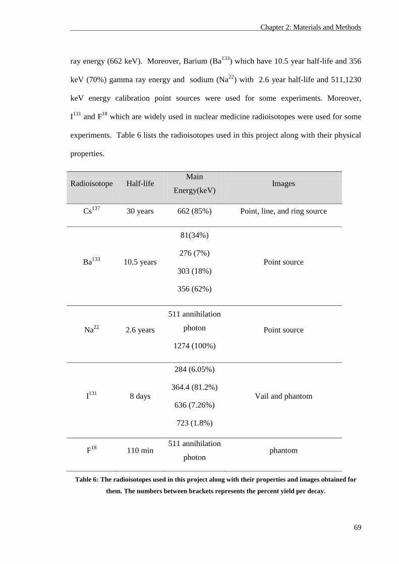
Chapter 2: Materials and Methods
69
ray energy (662 keV). Moreover, Barium (Ba133
) which have 10.5 year half-life and 356
keV (70%) gamma ray energy and sodium (Na22
) with 2.6 year half-life and 511,1230
keV energy calibration point sources were used for some experiments. Moreover,
I131
and F18
which are widely used in nuclear medicine radioisotopes were used for some
experiments. Table 6 lists the radioisotopes used in this project along with their physical
properties.
Radioisotope Half-life Main
Energy(keV) Images
Cs137
30 years 662 (85%) Point, line, and ring source
Ba133
10.5 years
81(34%)
276 (7%)
303 (18%)
356 (62%)
Point source
Na22
2.6 years
511 annihilation
photon
1274 (100%)
Point source
I131
8 days
284 (6.05%)
364.4 (81.2%)
636 (7.26%)
723 (1.8%)
Vail and phantom
F18
110 min 511 annihilation
photon phantom
Table 6: The radioisotopes used in this project along with their properties and images obtained for
them. The numbers between brackets represents the percent yield per decay.
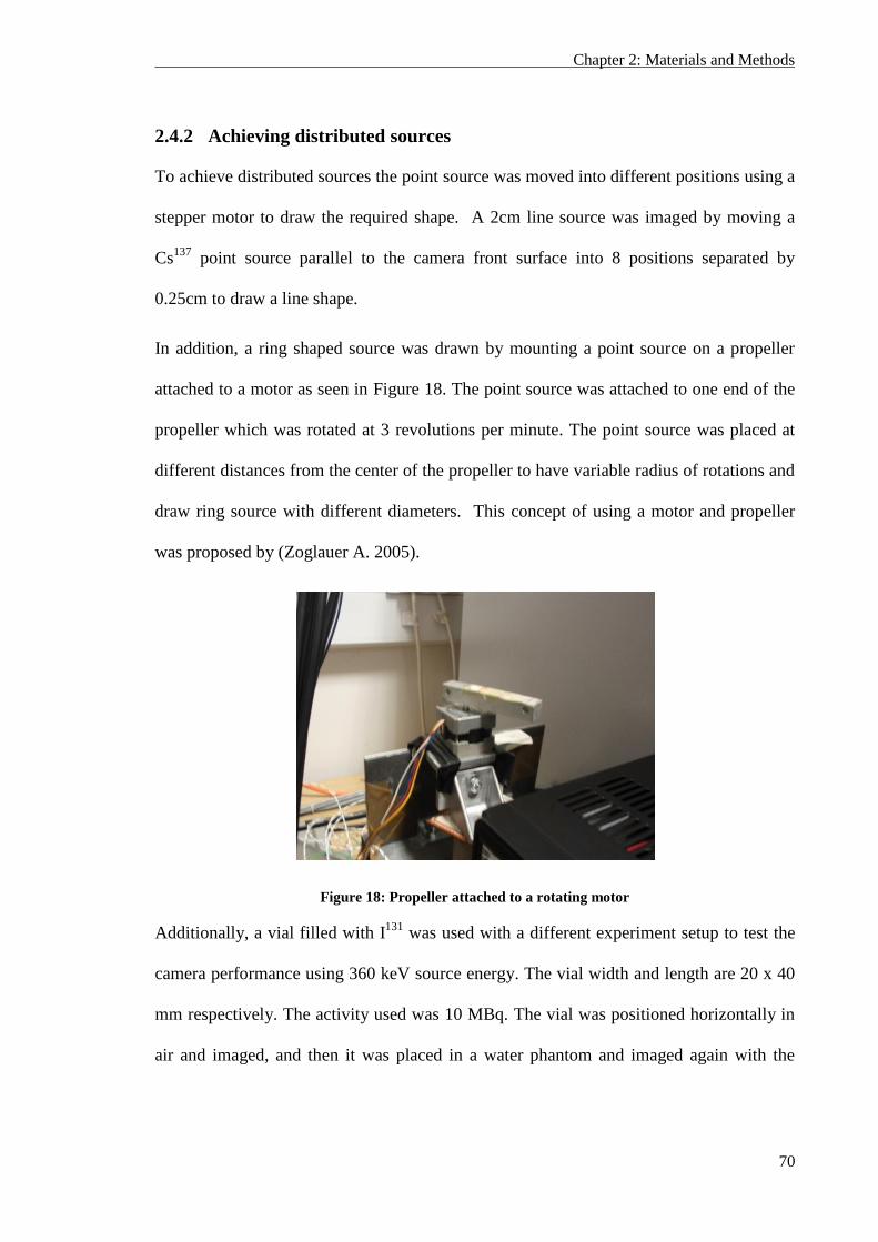
Chapter 2: Materials and Methods
70
2.4.2 Achieving distributed sources
To achieve distributed sources the point source was moved into different positions using a
stepper motor to draw the required shape. A 2cm line source was imaged by moving a
Cs137
point source parallel to the camera front surface into 8 positions separated by
0.25cm to draw a line shape.
In addition, a ring shaped source was drawn by mounting a point source on a propeller
attached to a motor as seen in Figure 18. The point source was attached to one end of the
propeller which was rotated at 3 revolutions per minute. The point source was placed at
different distances from the center of the propeller to have variable radius of rotations and
draw ring source with different diameters. This concept of using a motor and propeller
was proposed by (Zoglauer A. 2005).
Figure 18: Propeller attached to a rotating motor
Additionally, a vial filled with I131
was used with a different experiment setup to test the
camera performance using 360 keV source energy. The vial width and length are 20 x 40
mm respectively. The activity used was 10 MBq. The vial was positioned horizontally in
air and imaged, and then it was placed in a water phantom and imaged again with the
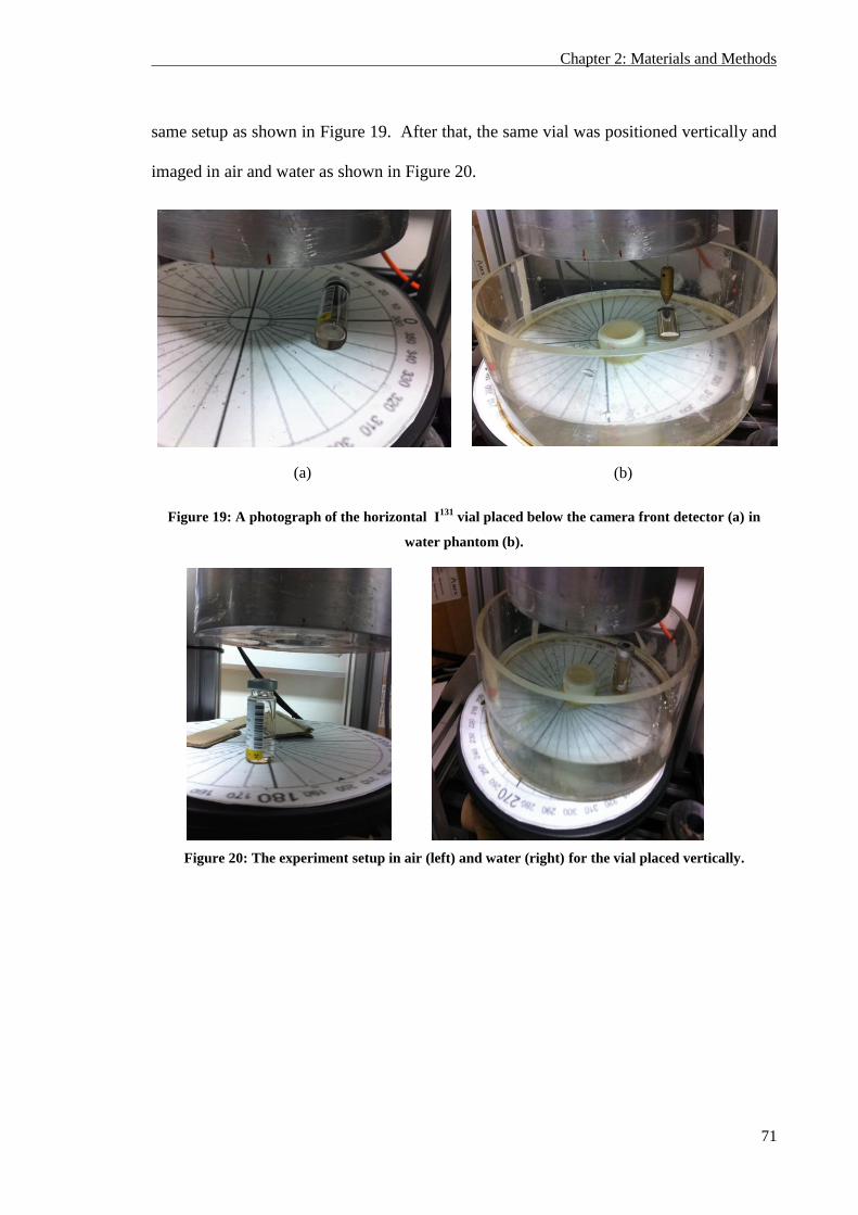
Chapter 2: Materials and Methods
71
same setup as shown in Figure 19. After that, the same vial was positioned vertically and
imaged in air and water as shown in Figure 20.
(a)
(b)
Figure 19: A photograph of the horizontal I131
vial placed below the camera front detector (a) in
water phantom (b).
Figure 20: The experiment setup in air (left) and water (right) for the vial placed vertically.
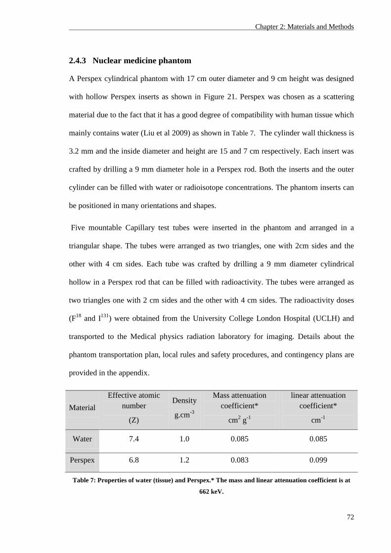
Chapter 2: Materials and Methods
72
2.4.3 Nuclear medicine phantom
A Perspex cylindrical phantom with 17 cm outer diameter and 9 cm height was designed
with hollow Perspex inserts as shown in Figure 21. Perspex was chosen as a scattering
material due to the fact that it has a good degree of compatibility with human tissue which
mainly contains water (Liu et al 2009) as shown in Table 7. The cylinder wall thickness is
3.2 mm and the inside diameter and height are 15 and 7 cm respectively. Each insert was
crafted by drilling a 9 mm diameter hole in a Perspex rod. Both the inserts and the outer
cylinder can be filled with water or radioisotope concentrations. The phantom inserts can
be positioned in many orientations and shapes.
Five mountable Capillary test tubes were inserted in the phantom and arranged in a
triangular shape. The tubes were arranged as two triangles, one with 2cm sides and the
other with 4 cm sides. Each tube was crafted by drilling a 9 mm diameter cylindrical
hollow in a Perspex rod that can be filled with radioactivity. The tubes were arranged as
two triangles one with 2 cm sides and the other with 4 cm sides. The radioactivity doses
(F18
and I131
) were obtained from the University College London Hospital (UCLH) and
transported to the Medical physics radiation laboratory for imaging. Details about the
phantom transportation plan, local rules and safety procedures, and contingency plans are
provided in the appendix.
Material
Effective atomic
number
(Z)
Density
g.cm-3
Mass attenuation
coefficient*
cm2 g
-1
linear attenuation
coefficient*
cm-1
Water 7.4 1.0 0.085 0.085
Perspex 6.8 1.2 0.083 0.099
Table 7: Properties of water (tissue) and Perspex.* The mass and linear attenuation coefficient is at
662 keV.
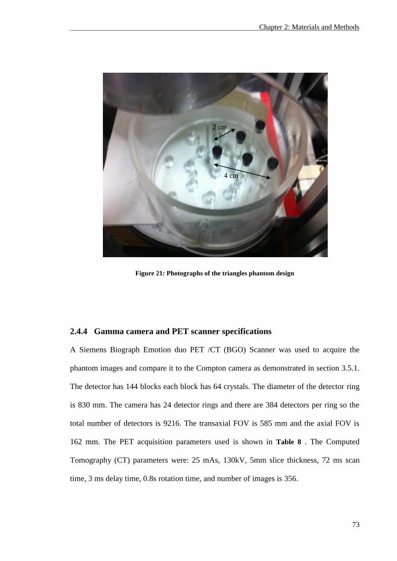
Chapter 2: Materials and Methods
73
Figure 21: Photographs of the triangles phantom design
2.4.4 Gamma camera and PET scanner specifications
A Siemens Biograph Emotion duo PET /CT (BGO) Scanner was used to acquire the
phantom images and compare it to the Compton camera as demonstrated in section 3.5.1.
The detector has 144 blocks each block has 64 crystals. The diameter of the detector ring
is 830 mm. The camera has 24 detector rings and there are 384 detectors per ring so the
total number of detectors is 9216. The transaxial FOV is 585 mm and the axial FOV is
162 mm. The PET acquisition parameters used is shown in Table 8 . The Computed
Tomography (CT) parameters were: 25 mAs, 130kV, 5mm slice thickness, 72 ms scan
time, 3 ms delay time, 0.8s rotation time, and number of images is 356.
4 cm
2 cm
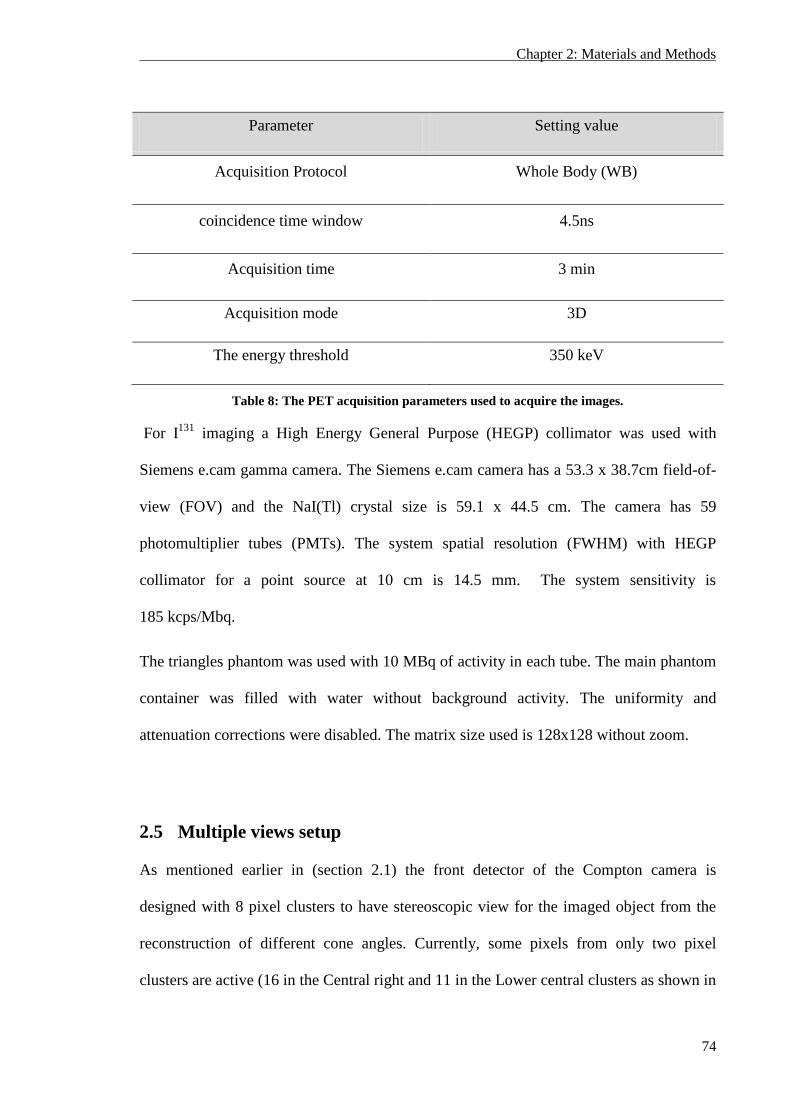
Chapter 2: Materials and Methods
74
Parameter Setting value
Acquisition Protocol Whole Body (WB)
coincidence time window 4.5ns
Acquisition time 3 min
Acquisition mode 3D
The energy threshold 350 keV
Table 8: The PET acquisition parameters used to acquire the images.
For I131
imaging a High Energy General Purpose (HEGP) collimator was used with
Siemens e.cam gamma camera. The Siemens e.cam camera has a 53.3 x 38.7cm field-of-
view (FOV) and the NaI(Tl) crystal size is 59.1 x 44.5 cm. The camera has 59
photomultiplier tubes (PMTs). The system spatial resolution (FWHM) with HEGP
collimator for a point source at 10 cm is 14.5 mm. The system sensitivity is
185 kcps/Mbq.
The triangles phantom was used with 10 MBq of activity in each tube. The main phantom
container was filled with water without background activity. The uniformity and
attenuation corrections were disabled. The matrix size used is 128x128 without zoom.
2.5 Multiple views setup
As mentioned earlier in (section 2.1) the front detector of the Compton camera is
designed with 8 pixel clusters to have stereoscopic view for the imaged object from the
reconstruction of different cone angles. Currently, some pixels from only two pixel
clusters are active (16 in the Central right and 11 in the Lower central clusters as shown in
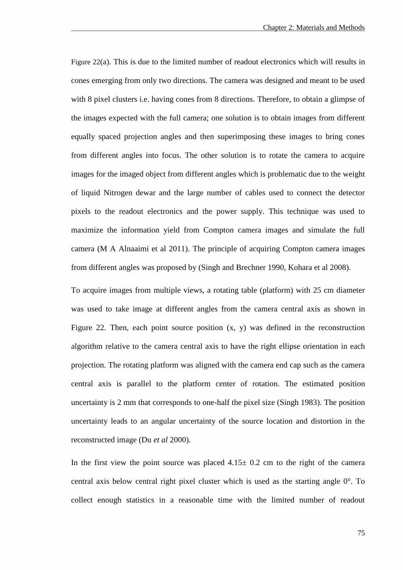
Chapter 2: Materials and Methods
75
Figure 22(a). This is due to the limited number of readout electronics which will results in
cones emerging from only two directions. The camera was designed and meant to be used
with 8 pixel clusters i.e. having cones from 8 directions. Therefore, to obtain a glimpse of
the images expected with the full camera; one solution is to obtain images from different
equally spaced projection angles and then superimposing these images to bring cones
from different angles into focus. The other solution is to rotate the camera to acquire
images for the imaged object from different angles which is problematic due to the weight
of liquid Nitrogen dewar and the large number of cables used to connect the detector
pixels to the readout electronics and the power supply. This technique was used to
maximize the information yield from Compton camera images and simulate the full
camera (M A Alnaaimi et al 2011). The principle of acquiring Compton camera images
from different angles was proposed by (Singh and Brechner 1990, Kohara et al 2008).
To acquire images from multiple views, a rotating table (platform) with 25 cm diameter
was used to take image at different angles from the camera central axis as shown in
Figure 22. Then, each point source position (x, y) was defined in the reconstruction
algorithm relative to the camera central axis to have the right ellipse orientation in each
projection. The rotating platform was aligned with the camera end cap such as the camera
central axis is parallel to the platform center of rotation. The estimated position
uncertainty is 2 mm that corresponds to one-half the pixel size (Singh 1983). The position
uncertainty leads to an angular uncertainty of the source location and distortion in the
reconstructed image (Du et al 2000).
In the first view the point source was placed 4.15± 0.2 cm to the right of the camera
central axis below central right pixel cluster which is used as the starting angle 0°. To
collect enough statistics in a reasonable time with the limited number of readout
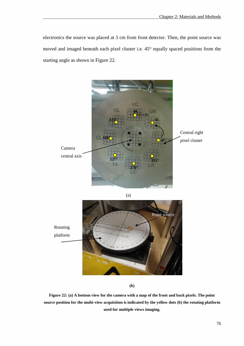
Chapter 2: Materials and Methods
76
electronics the source was placed at 3 cm from front detector. Then, the point source was
moved and imaged beneath each pixel cluster i.e. 45° equally spaced positions from the
starting angle as shown in Figure 22.
(b)
Figure 22: (a) A bottom view for the camera with a map of the front and back pixels. The point
source position for the multi-view acquisition is indicated by the yellow dots (b) the rotating platform
used for multiple views imaging.
(a)
4.15 cm
0°
45
°
90
° 135°
180°
227°
270°
315°
Central right
pixel cluster
Camera
central axis
Point source
Rotating
platform
Chapter 2: Materials and Methods
77
2.6 Data analysis
Proper evaluation of the imaging system performance is required to have a fair
comparison of Compton camera to conventional cameras. Predicting system performance
accurately is critical in imaging system design. System geometry and system parameters
can be optimized and determined accordingly before actual hardware implementation.
Nuclear medicine imaging systems are often described in terms of physical quantities that
characterize various aspects of their performance. These quantities include measures of
spatial resolution, signal to noise ratio, and contrast as described in the following
paragraphs.
Point spread function (PSF)
Line profile was taken across the imaged point source and the FWHM of the profile was
measured by taking the width of half the peak maximum value. In some experiment
asymmetric pixels geometry was used which results in non-uniform cone shapes and
directions, thus, the average PSF for the line profiles taken from different angles through
the imaged source was taken. The PSF is used in chapter 3 to evaluate the spatial spread
of the point source images obtained at different distances and variable source energies.
Signal to noise ratio (SNR)
The SNR was calculated within a circular region of interest ROI (1cm diameter) which
was defined in the center of each image around the imaged source within which the mean
was divided by standard deviation (Dahlbom et al 2005). The SNR was used to evaluate
the count rate performance and the effect of noise on the point, line, ring and phantom
images presented in chapter 3. It is assumed that the image noise originates from the
Chapter 2: Materials and Methods
78
statistical noise in the counting data (Sorenson and Phelps 1987). The SNR increases as
the total counts increase and decreases as the number of image pixels increases.
Percentage contrast
The contrast of the image which refers to the difference in intensity in parts of the image
related to different concentrations of activity (Sorenson & Phelps 1987) was measured by
using (22):
(22)
Where max and min refers to the maximum and minimum pixel value. The results were
multiplied by 100 to obtain the percentage contrast.
2.7 Image acquisition
To controls the readout electronics and data acquisition the MIDAS (Multi Instance Data
Acquisition System) acquisition software developed by V. Pucknell (2004) was used. The
GRT4 VME modules are configured, controlled and monitored by the MIDAS software.
The experiment setup can be saved and used by the automatic experiment control in order
to restore the hardware to its predefined state. The MWD energy determination algorithm
parameters can be defined in the MIDAS software as well as the CFD and trigger values.
The MIDAS software communicate with GRT4 cards via the Power PC and receives a
block of data that contains the trace of each pixel which is then recorded it in a tape
storage media for offline analysis.
Chapter 2: Materials and Methods
79
2.8 Errors
All measurements are subject to errors which can be systematic or statistical. Systematic
errors are those caused by incorrect settings and produce results that consistently differ
from the correct result by some fixed amount. Random error on the other hand is the
variation in the results from one measurement to another due to the physical limitation of
the system or from the actual random variations of the measured quantity itself (Sorenson
and Phelps 1987). The inherent measurement position and energy errors results in a miss-
estimation of the cone parameters which eventually lead to a density distribution about
the true location of the point of emission (Solomon and R J Ott 1988).
Some possible sources of errors in this work include: positioning, random and
backprojection reconstruction errors. Positioning error is caused by the uncertainty in the
exact position of the front and back pixels relative to the source position. The pixel is
assumed to be within half a pixel size (± 2 mm) of its nominal position (Singh 1983).
Positioning errors lead to source to detector alignment errors. The back projection
algorithm is sensitive to the errors in detector and source alignment i.e. small
misalignment can cause large distortion in the reconstructed image (Du et al 2000).
Random errors in the measurement arise from the inherent counting fluctuations due to
the random nature of radioactive decay and the statistical variation of the number of
charge carriers produced for an incident photon (Knoll 1999).
In addition, the intersection of the backprojected ellipses and the source plane results in
image error (artifacts). This artifact can be defined as the extra unwanted information that
is artificially produced by the reconstruction algorithm that the original imaged object did
not contain (Ahmed 2007).
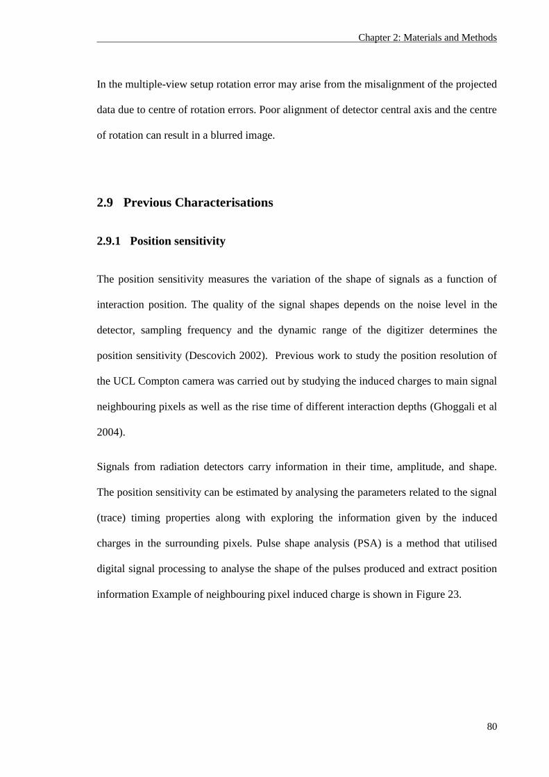
Chapter 2: Materials and Methods
80
In the multiple-view setup rotation error may arise from the misalignment of the projected
data due to centre of rotation errors. Poor alignment of detector central axis and the centre
of rotation can result in a blurred image.
2.9 Previous Characterisations
2.9.1 Position sensitivity
The position sensitivity measures the variation of the shape of signals as a function of
interaction position. The quality of the signal shapes depends on the noise level in the
detector, sampling frequency and the dynamic range of the digitizer determines the
position sensitivity (Descovich 2002). Previous work to study the position resolution of
the UCL Compton camera was carried out by studying the induced charges to main signal
neighbouring pixels as well as the rise time of different interaction depths (Ghoggali et al
2004).
Signals from radiation detectors carry information in their time, amplitude, and shape.
The position sensitivity can be estimated by analysing the parameters related to the signal
(trace) timing properties along with exploring the information given by the induced
charges in the surrounding pixels. Pulse shape analysis (PSA) is a method that utilised
digital signal processing to analyse the shape of the pulses produced and extract position
information Example of neighbouring pixel induced charge is shown in Figure 23.
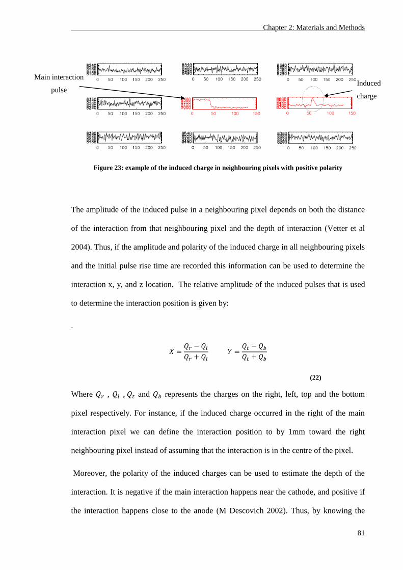
Chapter 2: Materials and Methods
81
Figure 23: example of the induced charge in neighbouring pixels with positive polarity
The amplitude of the induced pulse in a neighbouring pixel depends on both the distance
of the interaction from that neighbouring pixel and the depth of interaction (Vetter et al
2004). Thus, if the amplitude and polarity of the induced charge in all neighbouring pixels
and the initial pulse rise time are recorded this information can be used to determine the
interaction x, y, and z location. The relative amplitude of the induced pulses that is used
to determine the interaction position is given by:
.
(22)
Where , , and represents the charges on the right, left, top and the bottom
pixel respectively. For instance, if the induced charge occurred in the right of the main
interaction pixel we can define the interaction position to by 1mm toward the right
neighbouring pixel instead of assuming that the interaction is in the centre of the pixel.
Moreover, the polarity of the induced charges can be used to estimate the depth of the
interaction. It is negative if the main interaction happens near the cathode, and positive if
the interaction happens close to the anode (M Descovich 2002). Thus, by knowing the
Main interaction
pulse Induced
charge
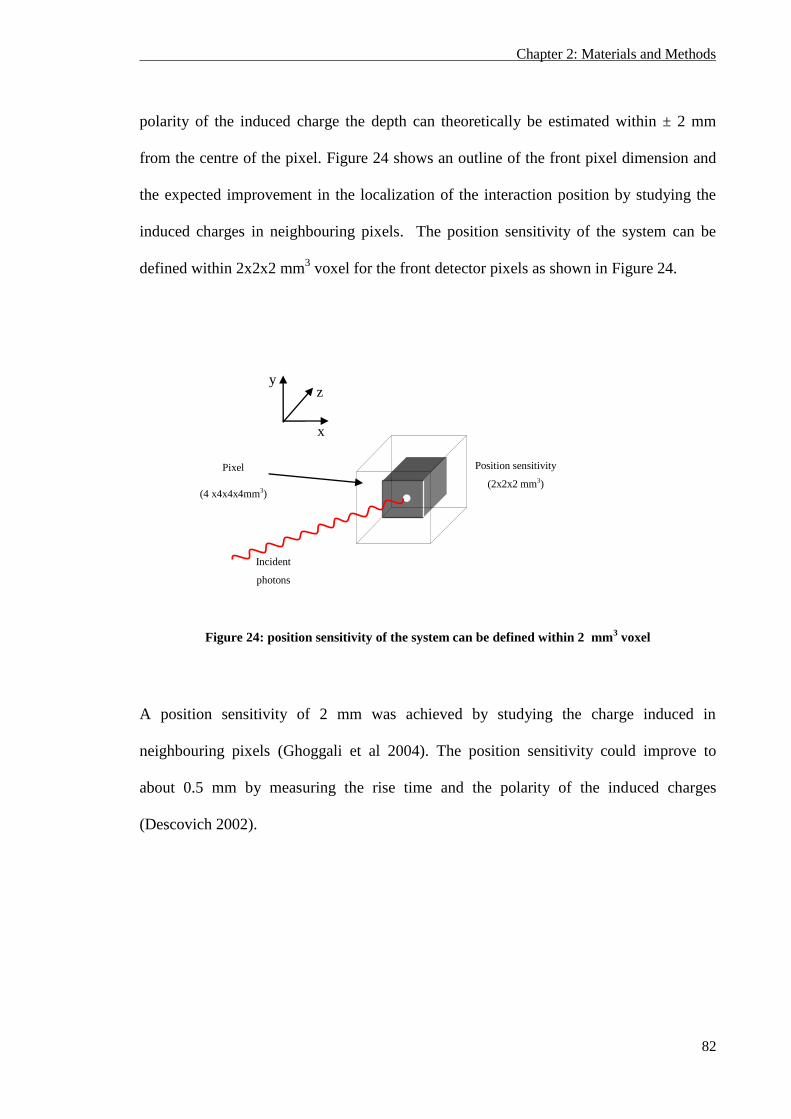
Chapter 2: Materials and Methods
82
polarity of the induced charge the depth can theoretically be estimated within ± 2 mm
from the centre of the pixel. Figure 24 shows an outline of the front pixel dimension and
the expected improvement in the localization of the interaction position by studying the
induced charges in neighbouring pixels. The position sensitivity of the system can be
defined within 2x2x2 mm3 voxel for the front detector pixels as shown in Figure 24.
Figure 24: position sensitivity of the system can be defined within 2 mm3 voxel
A position sensitivity of 2 mm was achieved by studying the charge induced in
neighbouring pixels (Ghoggali et al 2004). The position sensitivity could improve to
about 0.5 mm by measuring the rise time and the polarity of the induced charges
(Descovich 2002).
x
y z
Pixel
(4 x4x4x4mm3)
Incident
photons
Position sensitivity
(2x2x2 mm3)
Chapter 2: Materials and Methods
83
2.9.2 Simulated efficiency
A Monte Carlo program (EGS4) was used to compute the UCL Compton camera
detection efficiency for a point source at 5 cm from the front detector surface (Royle et al
2003). An estimation of the efficiency of the camera has been computed using (15) by
considering the various interaction probabilities and solid angles for a gamma ray emitted
by the source and then Compton scattered in one of the front detector pixels followed by
an absorption in one of the back detector pixels.
It should be noticed that the simulated efficiency was done for the full system i.e. 152
front pixels and 25 back pixels. The Compton camera efficiency for different source
energies is shown in Figure 25.
Figure 25: simulated efficiency of the UCL Compton camera for a point source at 5 cm from the front
camera face (G J Royle et al 2003).
As can be seen in Figure 25 the absolute efficiency computed from Monte Carlo
simulation was estimated to range from 3.6x10-04
to 3.06 x10-05
for 140 and 662 keV
respectively. The absolute efficiency of Compton camera shown in Figure 25 for the
0.00E+00
5.00E-05
1.00E-04
1.50E-04
2.00E-04
2.50E-04
3.00E-04
3.50E-04
0 100 200 300 400 500 600 700
Eff
icie
ncy
Source energy (keV)
Chapter 2: Materials and Methods
84
energy range 140 to 662 keV is comparable with that of conventional SPECT gamma
cameras (1.9 x10⁻⁴
and 4.2x10⁻⁴
) as reported by (Madsen 2007).
The efficiency of the camera could be improved by increasing the mass of detector
elements in the front detector; however this would increase the cost due to the additional
readout electronics. The low UCL camera efficiency compared to the Compton camera
developed by (J. B Martin et al 1993, Du et al 2001) is mainly due to the large separation
between the two detectors and their geometrical arrangement. The efficiency decreases
exponentially with increasing the separation between the detectors (Martin et al 1994)
The back detector has smaller detection area than the front detector and subtended a small
angular range, thus suffers from low efficiency. The reason of having larger front detector
backed by a smaller one is to maximise the depth resolution as described in (section 2.1)
Chapter 3: Results and Discussions
85
Chapter 3
3 Results and Discussions
This chapter contains a description of the system performance characteristics and imaging
performance. In the beginning of this chapter the probability of interaction of incoming
photons with the camera will be presented. Then, the effect of random events on the
camera and how to minimise it will be described. The system performance characteristics
in terms of resolution, efficiency, and counting performance are presented. The imaging
performance of the UCL Compton camera with extended source distributions was
evaluated. A quantitative analysis of the experimental results is given and discussed.
Moreover, a multiple views technique was used to simulate the full system. The camera
resolving power was measured and reported. Finally, phantom images were acquired and
compared to SPECT and PET.
3.1 Probability of interaction
In Compton camera systems it is required to maximize the probability of single Compton
interaction in the front detector followed by an escape and total energy deposition in the
back detector (Singh 1983). This requires that the back detector subtend a large solid
angle at the first detector and also the back detector need to be thick enough to stop the
scattered photons. The probability of interaction of photons with the front and back
detector was investigated to have more understanding for the amount for energy deposited
in each detector and its relation with the source energy. With the scatter (front) detector
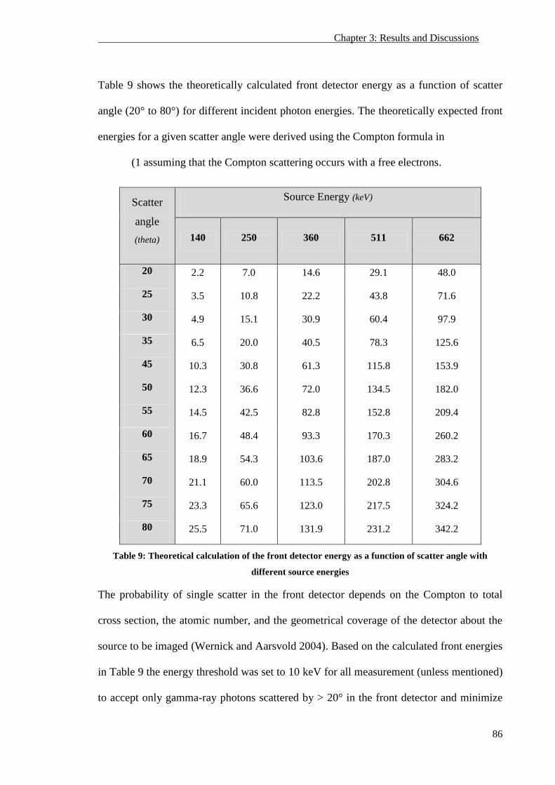
Chapter 3: Results and Discussions
86
Table 9 shows the theoretically calculated front detector energy as a function of scatter
angle (20° to 80°) for different incident photon energies. The theoretically expected front
energies for a given scatter angle were derived using the Compton formula in
(1 assuming that the Compton scattering occurs with a free electrons.
Scatter
angle
(theta)
Source Energy (keV)
140 250 360 511 662
20 2.2 7.0 14.6 29.1 48.0
25 3.5 10.8 22.2 43.8 71.6
30 4.9 15.1 30.9 60.4 97.9
35 6.5 20.0 40.5 78.3 125.6
45 10.3 30.8 61.3 115.8 153.9
50 12.3 36.6 72.0 134.5 182.0
55 14.5 42.5 82.8 152.8 209.4
60 16.7 48.4 93.3 170.3 260.2
65 18.9 54.3 103.6 187.0 283.2
70 21.1 60.0 113.5 202.8 304.6
75 23.3 65.6 123.0 217.5 324.2
80 25.5 71.0 131.9 231.2 342.2
Table 9: Theoretical calculation of the front detector energy as a function of scatter angle with
different source energies
The probability of single scatter in the front detector depends on the Compton to total
cross section, the atomic number, and the geometrical coverage of the detector about the
source to be imaged (Wernick and Aarsvold 2004). Based on the calculated front energies
in Table 9 the energy threshold was set to 10 keV for all measurement (unless mentioned)
to accept only gamma-ray photons scattered by > 20° in the front detector and minimize
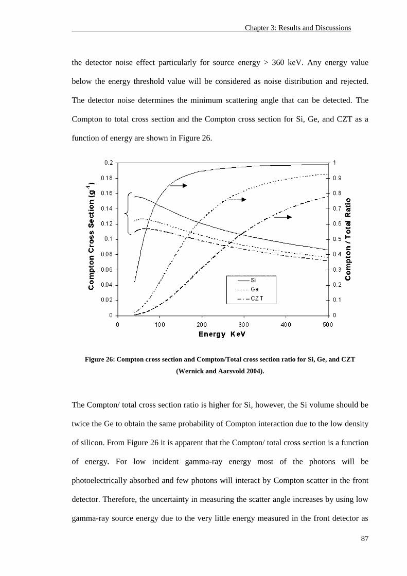
Chapter 3: Results and Discussions
87
the detector noise effect particularly for source energy > 360 keV. Any energy value
below the energy threshold value will be considered as noise distribution and rejected.
The detector noise determines the minimum scattering angle that can be detected. The
Compton to total cross section and the Compton cross section for Si, Ge, and CZT as a
function of energy are shown in Figure 26.
Figure 26: Compton cross section and Compton/Total cross section ratio for Si, Ge, and CZT
(Wernick and Aarsvold 2004).
The Compton/ total cross section ratio is higher for Si, however, the Si volume should be
twice the Ge to obtain the same probability of Compton interaction due to the low density
of silicon. From Figure 26 it is apparent that the Compton/ total cross section is a function
of energy. For low incident gamma-ray energy most of the photons will be
photoelectrically absorbed and few photons will interact by Compton scatter in the front
detector. Therefore, the uncertainty in measuring the scatter angle increases by using low
gamma-ray source energy due to the very little energy measured in the front detector as
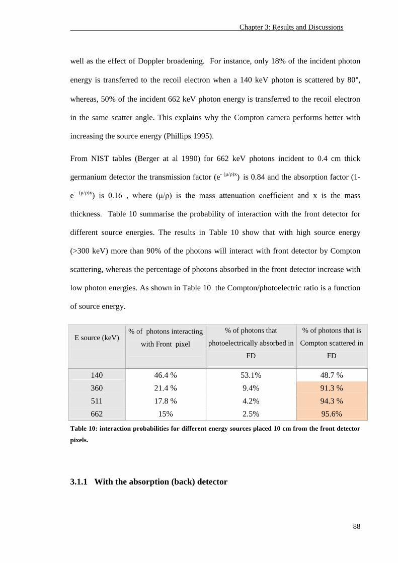
Chapter 3: Results and Discussions
88
well as the effect of Doppler broadening. For instance, only 18% of the incident photon
energy is transferred to the recoil electron when a 140 keV photon is scattered by 80°,
whereas, 50% of the incident 662 keV photon energy is transferred to the recoil electron
in the same scatter angle. This explains why the Compton camera performs better with
increasing the source energy (Phillips 1995).
From NIST tables (Berger at al 1990) for 662 keV photons incident to 0.4 cm thick
germanium detector the transmission factor (e- (μ/ρ)x
) is 0.84 and the absorption factor (1-
e- (μ/ρ)x
) is 0.16 , where (μ/ρ) is the mass attenuation coefficient and x is the mass
thickness. Table 10 summarise the probability of interaction with the front detector for
different source energies. The results in Table 10 show that with high source energy
(>300 keV) more than 90% of the photons will interact with front detector by Compton
scattering, whereas the percentage of photons absorbed in the front detector increase with
low photon energies. As shown in Table 10 the Compton/photoelectric ratio is a function
of source energy.
E source (keV)
% of photons interacting
with Front pixel
% of photons that
photoelectrically absorbed in
FD
% of photons that is
Compton scattered in
FD
140 46.4 % 53.1% 48.7 %
360 21.4 % 9.4% 91.3 %
511 17.8 % 4.2% 94.3 %
662 15% 2.5% 95.6%
Table 10: interaction probabilities for different energy sources placed 10 cm from the front detector
pixels.
3.1.1 With the absorption (back) detector
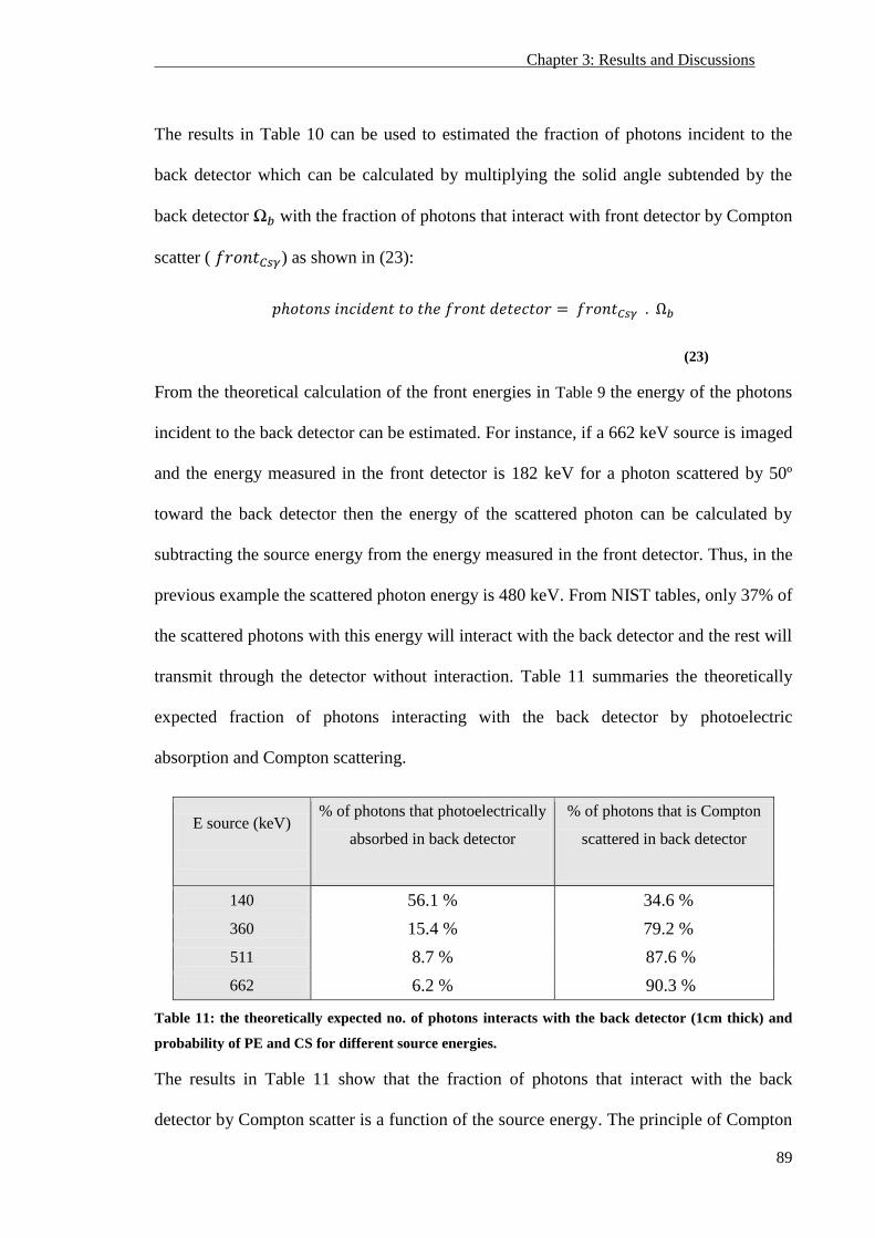
Chapter 3: Results and Discussions
89
The results in Table 10 can be used to estimated the fraction of photons incident to the
back detector which can be calculated by multiplying the solid angle subtended by the
back detector with the fraction of photons that interact with front detector by Compton
scatter ( ) as shown in (23):
(23)
From the theoretical calculation of the front energies in Table 9 the energy of the photons
incident to the back detector can be estimated. For instance, if a 662 keV source is imaged
and the energy measured in the front detector is 182 keV for a photon scattered by 50º
toward the back detector then the energy of the scattered photon can be calculated by
subtracting the source energy from the energy measured in the front detector. Thus, in the
previous example the scattered photon energy is 480 keV. From NIST tables, only 37% of
the scattered photons with this energy will interact with the back detector and the rest will
transmit through the detector without interaction. Table 11 summaries the theoretically
expected fraction of photons interacting with the back detector by photoelectric
absorption and Compton scattering.
E source (keV)
% of photons that photoelectrically
absorbed in back detector
% of photons that is Compton
scattered in back detector
140 56.1 % 34.6 %
360 15.4 % 79.2 %
511 8.7 % 87.6 %
662 6.2 % 90.3 %
Table 11: the theoretically expected no. of photons interacts with the back detector (1cm thick) and
probability of PE and CS for different source energies.
The results in Table 11 show that the fraction of photons that interact with the back
detector by Compton scatter is a function of the source energy. The principle of Compton
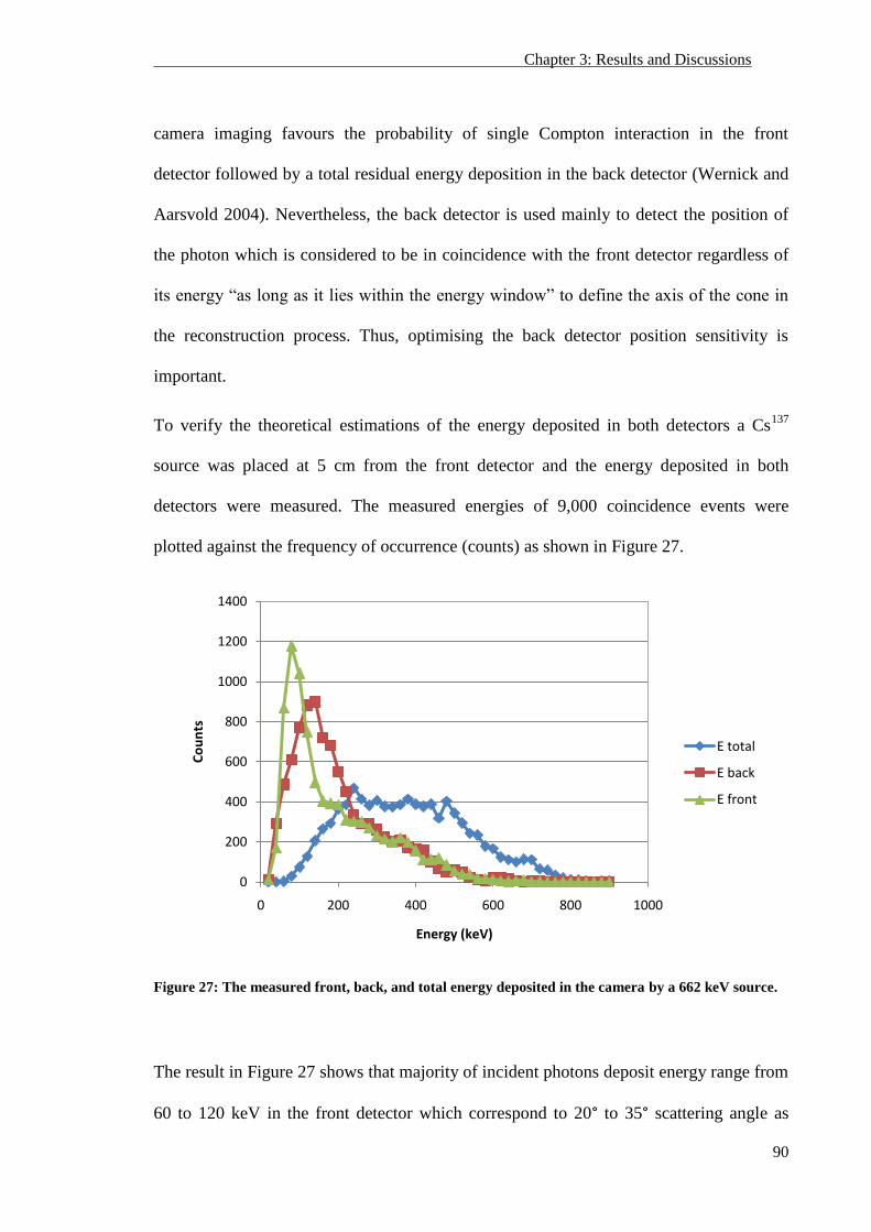
Chapter 3: Results and Discussions
90
camera imaging favours the probability of single Compton interaction in the front
detector followed by a total residual energy deposition in the back detector (Wernick and
Aarsvold 2004). Nevertheless, the back detector is used mainly to detect the position of
the photon which is considered to be in coincidence with the front detector regardless of
its energy “as long as it lies within the energy window” to define the axis of the cone in
the reconstruction process. Thus, optimising the back detector position sensitivity is
important.
To verify the theoretical estimations of the energy deposited in both detectors a Cs137
source was placed at 5 cm from the front detector and the energy deposited in both
detectors were measured. The measured energies of 9,000 coincidence events were
plotted against the frequency of occurrence (counts) as shown in Figure 27.
Figure 27: The measured front, back, and total energy deposited in the camera by a 662 keV source.
The result in Figure 27 shows that majority of incident photons deposit energy range from
60 to 120 keV in the front detector which correspond to 20° to 35° scattering angle as
0
200
400
600
800
1000
1200
1400
0 200 400 600 800 1000
Co
un
ts
Energy (keV)
E total
E back
E front
Chapter 3: Results and Discussions
91
shown in Table 9. In average the measured front energy is about only 18 % of the source
energy due to the small detector thickness (4 mm). The measured energy in the back
detector shows that the photons incident to the back detector deposit only part of its
energy range from 120 to 160 keV (~ 20 % of source energy). Note that higher energies
were recorded in the back detector compared to the front detector due to its 10 mm
thickness.
The total energy measured for every coincidence event shows that with 662 keV source
most of coincidence photons escape without full deposition of its energy. The result in
Figure 27 shows that the majority of the events deposit total energy which range from 220
to 440 keV in both detectors. Thus, wide energy window width was used to avoid loss of
useful true events as discussed in section ( 2.2.3) the energy window was set to 450 keV
for 662 keV photons imaging. Possible reason of incomplete energy deposition in the
detectors is the high source energy used for this analysis (662 keV) compared to the small
thickness of the detectors (4 and 10 mm). Therefore, the incident photons have high
Compton scatter probability in both detectors, as indicated earlier, and loss only part of its
energy rather than its total energy.
3.1.2 Random coincidence in Compton camera
The method of coincidence detection used in Compton camera has an obstacle (similar to
PET) in that two unrelated photons might accepted simultaneously within the same
coincidence timing window mainly due to the finite uncertainty in the time of arrival of a
photon at the detector (Webb 1988). These events are called random (accidental) events.
The direct consequence of random events is the addition of noise to the measured data
due to the inaccurate assignment of the lines of response in PET and cone axis parameters
Chapter 3: Results and Discussions
92
in Compton camera. It is difficult to distinguish a random from a genuine coincidence
event (Webb 1988). The random events increase as the square of source activity
(Budinger 1998). Correction of random events is the focus of ongoing research in PET
(Rahmim and Zaidi 2008). Mathematically, the random events rate for a particular LOR
connecting to detectors i and j is given by:
(24)
Where τ is the coincidence time window and Si and Sj refer to the singles rates at the two
detectors (Rahmim and Zaidi 2008). The conventional approach to correct for random
events in PET is to observe the rate of events in a second delayed-coincidence window
and subtract the estimate of the random from the measured coincidence. However, this
approach does not remove and increases the noise in the data along with producing data
which is no longer Poisson distributed (Rahmim and Zaidi 2008). Alternatively, an
average estimate of the single rates can be modelled and included in the image
reconstruction task to avoid the problem associated with the subtraction technique (Oliver
and Rafecas 2010). The estimate of singles rate and the expected random events can be
calculated using (24). The single rate estimation method has less noise than the delayed
window method because it uses exclusively true coincidence counts. Effort is needed to
implement and develop random events correction techniques for Compton camera data.
The geometrical arrangement of the camera (refer to section 2.1) impose a limitation at
high counting rate in that the rate of single events in the back detector becomes
prohibitive. The single events have two main effects: the first is the increase in the system
dead time due to the time needed to process the high number of events collected. The
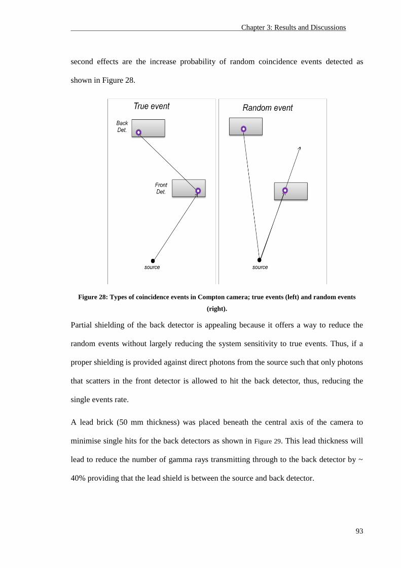
Chapter 3: Results and Discussions
93
second effects are the increase probability of random coincidence events detected as
shown in Figure 28.
Figure 28: Types of coincidence events in Compton camera; true events (left) and random events
(right).
Partial shielding of the back detector is appealing because it offers a way to reduce the
random events without largely reducing the system sensitivity to true events. Thus, if a
proper shielding is provided against direct photons from the source such that only photons
that scatters in the front detector is allowed to hit the back detector, thus, reducing the
single events rate.
A lead brick (50 mm thickness) was placed beneath the central axis of the camera to
minimise single hits for the back detectors as shown in Figure 29. This lead thickness will
lead to reduce the number of gamma rays transmitting through to the back detector by ~
40% providing that the lead shield is between the source and back detector.
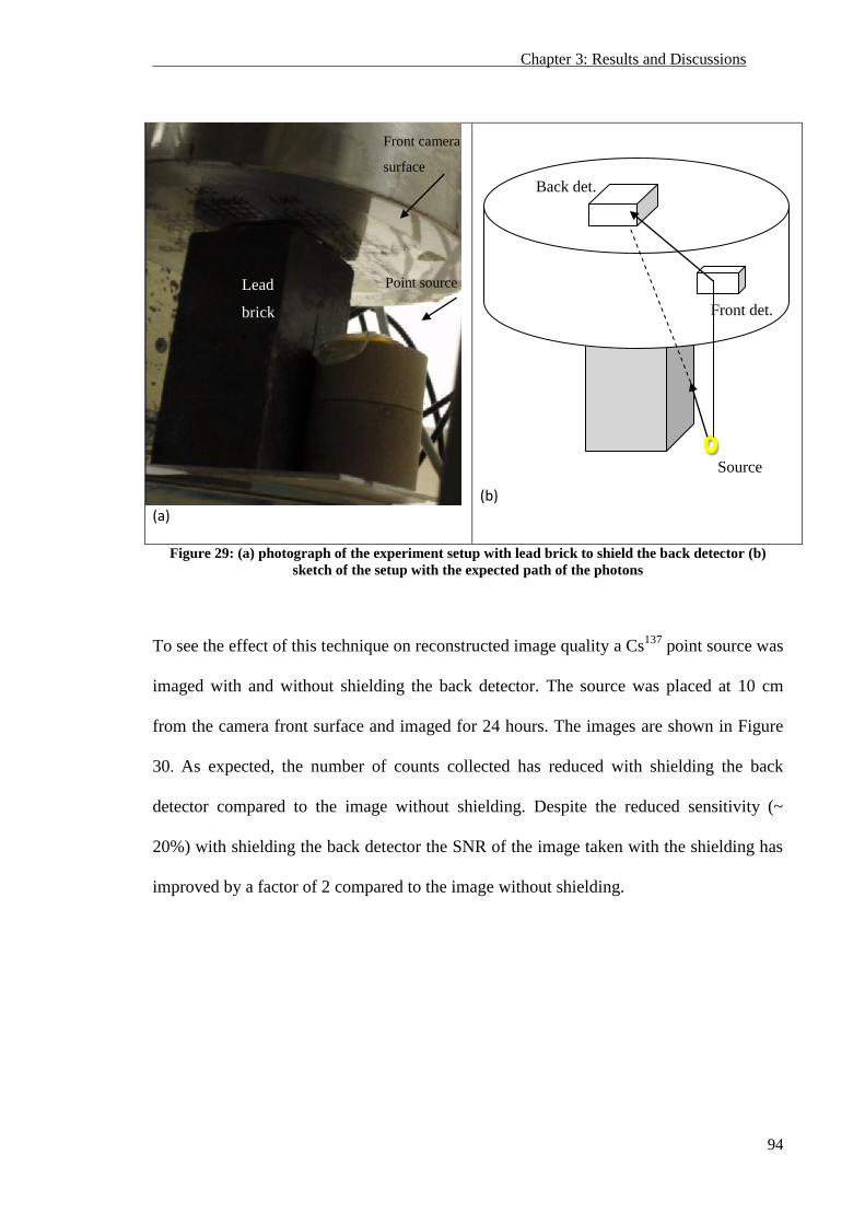
Chapter 3: Results and Discussions
94
(a)
(b)
Figure 29: (a) photograph of the experiment setup with lead brick to shield the back detector (b)
sketch of the setup with the expected path of the photons
To see the effect of this technique on reconstructed image quality a Cs137
point source was
imaged with and without shielding the back detector. The source was placed at 10 cm
from the camera front surface and imaged for 24 hours. The images are shown in Figure
30. As expected, the number of counts collected has reduced with shielding the back
detector compared to the image without shielding. Despite the reduced sensitivity (~
20%) with shielding the back detector the SNR of the image taken with the shielding has
improved by a factor of 2 compared to the image without shielding.
Lead
brick
Front camera
surface
Source
Front det.
Back det.
Point source
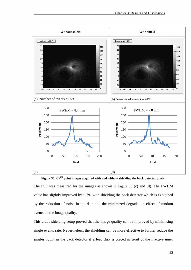
Chapter 3: Results and Discussions
95
Without shield With shield
(a) Number of events = 5599
(b) Number of events = 4491
(c)
(d)
Figure 30: Cs137
point images acquired with and without shielding the back detector pixels.
The PSF was measured for the images as shown in Figure 30 (c) and (d). The FWHM
value has slightly improved by ~ 7% with shielding the back detector which is explained
by the reduction of noise in the data and the minimized degradation effect of random
events on the image quality.
This crude shielding setup proved that the image quality can be improved by minimising
single events rate. Nevertheless, the shielding can be more effective to further reduce the
singles count in the back detector if a lead disk is placed in front of the inactive inner
0
50
100
150
200
250
300
0 50 100 150 200
Pix
el v
alu
e
Pixel
0
50
100
150
200
250
300
0 50 100 150 200
Pix
el v
alu
e
Pixel
FWHM = 8.4 mm FWHM = 7.8 mm
Chapter 3: Results and Discussions
96
region of the front detector such that the lead shield is placed between the source and the
back detector (Royle et al 2004).
Since the geometrical coverage of the camera decreases with extended source
distribution, a higher fraction of the singles is expected to hit the back detector.
Consequently, the partial shielding technique becomes less effective and depends on the
source geometry. Proper modelling of the estimated singles with different source
distributions (to include it in the reconstruction task) such that the estimation is
independent of the source geometry is required. Singles rate approximation becomes
more correct with extended source (Oliver and Rafecas 2010). Therefore, appropriate
estimation of random coincidence and their enclosure in the image reconstruction
algorithm can remove the bias in the images and minimize the noise amplification in the
data without altering the camera geometry (Rahmim and Zaidi 2008).

Chapter 3: Results and Discussions
97
3.2 System performance characterises
There are several factors that define the performance characteristics of the Compton
camera. These can be classified into hardware, software and physics related factors. The
hardware factors include the detector materials, geometry, and the readout electronics.
The physics related factors include the Doppler effects, random/true coincidence ratio,
and multiple Compton scatter issues. In addition, the characteristics of the software used
to process and reconstruct data are another factor that influences the system performance
because they play an important role in defining the image quality. The technicalities of
the Compton camera cannot be fully understood nor be optimized for clinical use, unless
these factors are addressed. In this section the main parameters that characterise the
system performance of the UCL prototype Compton camera will be demonstrated.
3.2.1 Energy resolution
To relate the energy of the incident radiation accurately with the signal detected by the
interaction of radiation with the detector the system was calibrated by acquiring gamma
ray photopeak spectra for different gamma ray energies. Two sources with different
energies (Ba133
and Cs137
) were used. The photopeak energies and their corresponding
ADC responses are fit with a linear gamma-ray energy calibration curve as shown in
Figure 31. Calibration curves were generated for all the pixels currently in use (31 pixels).
Slight variation (about 0.8 keV) was noticed from pixel to pixel which might be due to the
fact that each pixel has an independent preamplifier and amplifier that result in slightly
different output.
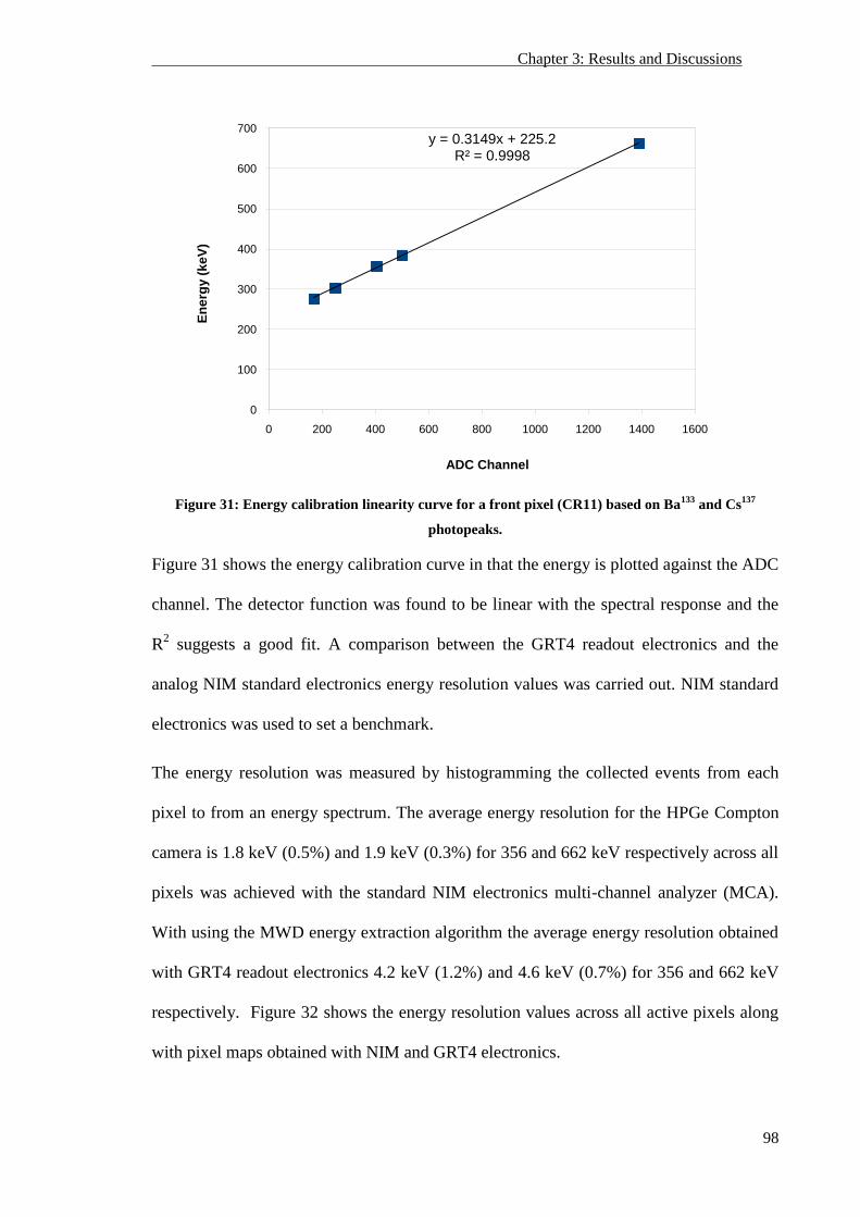
Chapter 3: Results and Discussions
98
Figure 31: Energy calibration linearity curve for a front pixel (CR11) based on Ba133
and Cs137
photopeaks.
Figure 31 shows the energy calibration curve in that the energy is plotted against the ADC
channel. The detector function was found to be linear with the spectral response and the
R2 suggests a good fit. A comparison between the GRT4 readout electronics and the
analog NIM standard electronics energy resolution values was carried out. NIM standard
electronics was used to set a benchmark.
The energy resolution was measured by histogramming the collected events from each
pixel to from an energy spectrum. The average energy resolution for the HPGe Compton
camera is 1.8 keV (0.5%) and 1.9 keV (0.3%) for 356 and 662 keV respectively across all
pixels was achieved with the standard NIM electronics multi-channel analyzer (MCA).
With using the MWD energy extraction algorithm the average energy resolution obtained
with GRT4 readout electronics 4.2 keV (1.2%) and 4.6 keV (0.7%) for 356 and 662 keV
respectively. Figure 32 shows the energy resolution values across all active pixels along
with pixel maps obtained with NIM and GRT4 electronics.
y = 0.3149x + 225.2R² = 0.9998
0
100
200
300
400
500
600
700
0 200 400 600 800 1000 1200 1400 1600
En
erg
y (
ke
V)
ADC Channel
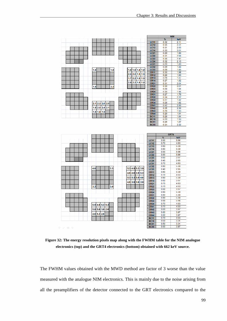
Chapter 3: Results and Discussions
99
Figure 32: The energy resolution pixels map along with the FWHM table for the NIM analogue
electronics (top) and the GRT4 electronics (bottom) obtained with 662 keV source.
The FWHM values obtained with the MWD method are factor of 3 worse than the value
measured with the analogue NIM electronics. This is mainly due to the noise arising from
all the preamplifiers of the detector connected to the GRT electronics compared to the
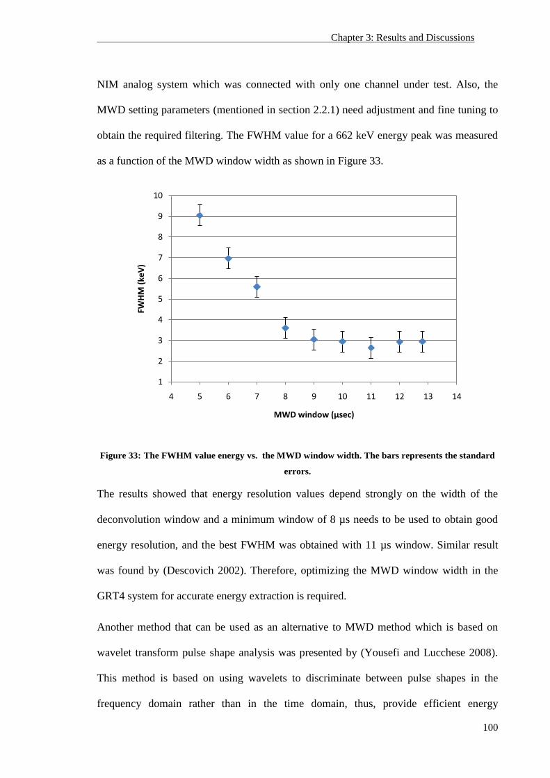
Chapter 3: Results and Discussions
100
NIM analog system which was connected with only one channel under test. Also, the
MWD setting parameters (mentioned in section 2.2.1) need adjustment and fine tuning to
obtain the required filtering. The FWHM value for a 662 keV energy peak was measured
as a function of the MWD window width as shown in Figure 33.
Figure 33: The FWHM value energy vs. the MWD window width. The bars represents the standard
errors.
The results showed that energy resolution values depend strongly on the width of the
deconvolution window and a minimum window of 8 µs needs to be used to obtain good
energy resolution, and the best FWHM was obtained with 11 µs window. Similar result
was found by (Descovich 2002). Therefore, optimizing the MWD window width in the
GRT4 system for accurate energy extraction is required.
Another method that can be used as an alternative to MWD method which is based on
wavelet transform pulse shape analysis was presented by (Yousefi and Lucchese 2008).
This method is based on using wavelets to discriminate between pulse shapes in the
frequency domain rather than in the time domain, thus, provide efficient energy
1
2
3
4
5
6
7
8
9
10
4 5 6 7 8 9 10 11 12 13 14
FWH
M (
keV
)
MWD window (µsec)
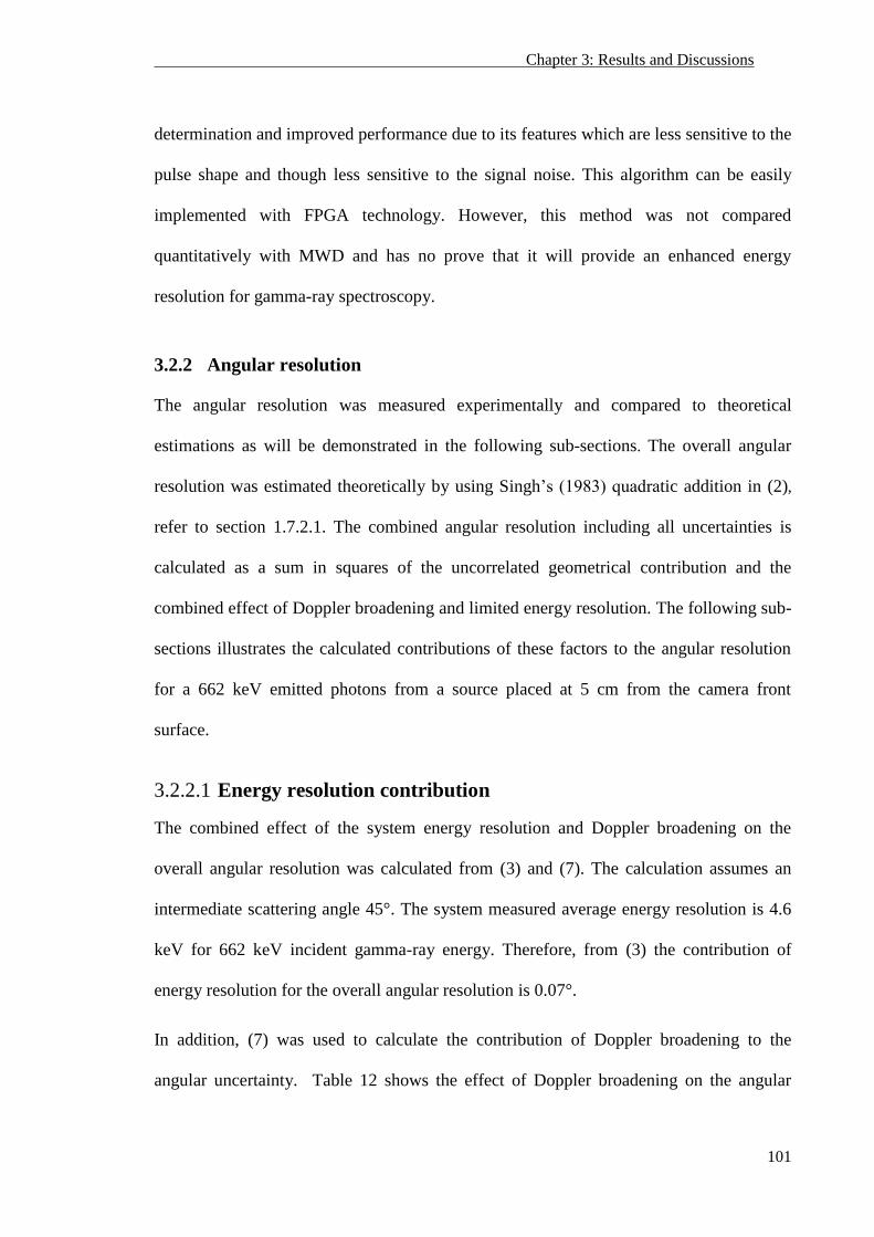
Chapter 3: Results and Discussions
101
determination and improved performance due to its features which are less sensitive to the
pulse shape and though less sensitive to the signal noise. This algorithm can be easily
implemented with FPGA technology. However, this method was not compared
quantitatively with MWD and has no prove that it will provide an enhanced energy
resolution for gamma-ray spectroscopy.
3.2.2 Angular resolution
The angular resolution was measured experimentally and compared to theoretical
estimations as will be demonstrated in the following sub-sections. The overall angular
resolution was estimated theoretically by using Singh’s (1983) quadratic addition in (2),
refer to section 1.7.2.1. The combined angular resolution including all uncertainties is
calculated as a sum in squares of the uncorrelated geometrical contribution and the
combined effect of Doppler broadening and limited energy resolution. The following sub-
sections illustrates the calculated contributions of these factors to the angular resolution
for a 662 keV emitted photons from a source placed at 5 cm from the camera front
surface.
3.2.2.1 Energy resolution contribution
The combined effect of the system energy resolution and Doppler broadening on the
overall angular resolution was calculated from (3) and (7). The calculation assumes an
intermediate scattering angle 45°. The system measured average energy resolution is 4.6
keV for 662 keV incident gamma-ray energy. Therefore, from (3) the contribution of
energy resolution for the overall angular resolution is 0.07°.
In addition, (7) was used to calculate the contribution of Doppler broadening to the
angular uncertainty. Table 12 shows the effect of Doppler broadening on the angular
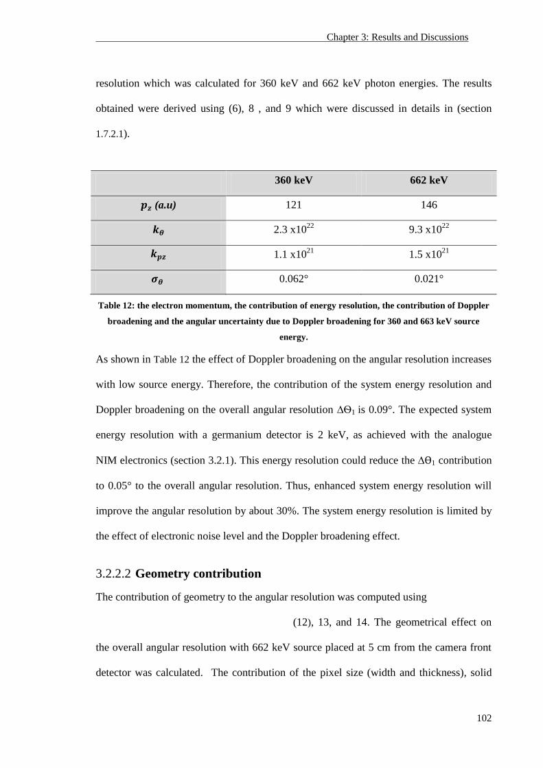
Chapter 3: Results and Discussions
102
resolution which was calculated for 360 keV and 662 keV photon energies. The results
obtained were derived using (6), 8 , and 9 which were discussed in details in (section
1.7.2.1).
360 keV 662 keV
(a.u) 121 146
2.3 x10²²
9.3 x10²²
1.1 x10²¹
1.5 x10²¹
0.062° 0.021°
Table 12: the electron momentum, the contribution of energy resolution, the contribution of Doppler
broadening and the angular uncertainty due to Doppler broadening for 360 and 663 keV source
energy.
As shown in Table 12 the effect of Doppler broadening on the angular resolution increases
with low source energy. Therefore, the contribution of the system energy resolution and
Doppler broadening on the overall angular resolution ∆Ѳ1 is 0.09°. The expected system
energy resolution with a germanium detector is 2 keV, as achieved with the analogue
NIM electronics (section 3.2.1). This energy resolution could reduce the ∆Ѳ1 contribution
to 0.05° to the overall angular resolution. Thus, enhanced system energy resolution will
improve the angular resolution by about 30%. The system energy resolution is limited by
the effect of electronic noise level and the Doppler broadening effect.
3.2.2.2 Geometry contribution
The contribution of geometry to the angular resolution was computed using
(12), 13, and 14. The geometrical effect on
the overall angular resolution with 662 keV source placed at 5 cm from the camera front
detector was calculated. The contribution of the pixel size (width and thickness), solid
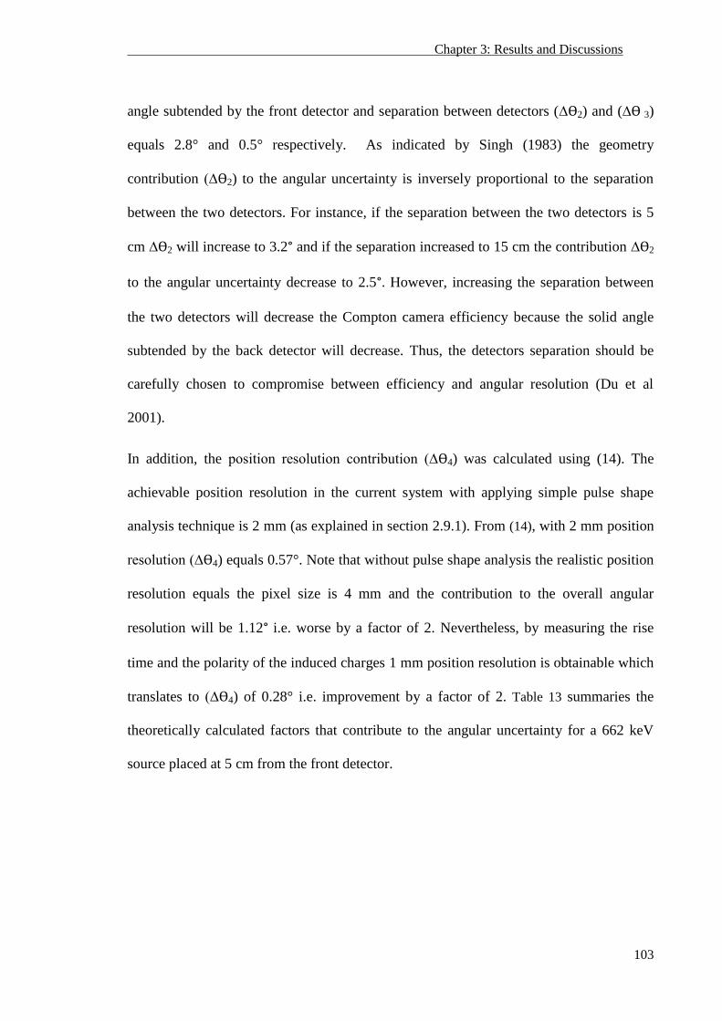
Chapter 3: Results and Discussions
103
angle subtended by the front detector and separation between detectors (∆Ѳ2) and (∆Ѳ 3)
equals 2.8° and 0.5° respectively. As indicated by Singh (1983) the geometry
contribution (∆Ѳ2) to the angular uncertainty is inversely proportional to the separation
between the two detectors. For instance, if the separation between the two detectors is 5
cm ∆Ѳ2 will increase to 3.2° and if the separation increased to 15 cm the contribution ∆Ѳ2
to the angular uncertainty decrease to 2.5°. However, increasing the separation between
the two detectors will decrease the Compton camera efficiency because the solid angle
subtended by the back detector will decrease. Thus, the detectors separation should be
carefully chosen to compromise between efficiency and angular resolution (Du et al
2001).
In addition, the position resolution contribution (∆Ѳ4) was calculated using (14). The
achievable position resolution in the current system with applying simple pulse shape
analysis technique is 2 mm (as explained in section 2.9.1). From (14), with 2 mm position
resolution (∆Ѳ4) equals 0.57°. Note that without pulse shape analysis the realistic position
resolution equals the pixel size is 4 mm and the contribution to the overall angular
resolution will be 1.12° i.e. worse by a factor of 2. Nevertheless, by measuring the rise
time and the polarity of the induced charges 1 mm position resolution is obtainable which
translates to (∆Ѳ4) of 0.28° i.e. improvement by a factor of 2. Table 13 summaries the
theoretically calculated factors that contribute to the angular uncertainty for a 662 keV
source placed at 5 cm from the front detector.
Chapter 3: Results and Discussions
104
Factor Angular uncertainty (degree)
Energy resolution ∆Ѳ1 0.09°
Geometry ∆Ѳ2 2.8 °
Geometry ∆Ѳ3 0.50 °
Position resolution ∆Ѳ4 0.57 °
Table 13: Summary of the calculated factors that contribute to the overall angular resolution using in
Singh’s quadratic equation for a 662 keV source placed at 5 cm.
As expected the effect of energy resolution is smaller than the geometrical effect due to
the excellent energy resolution of the germanium detector. From Table 13, the
theoretically calculated angular resolution for 662 keV source placed at 5 cm from the
camera front detector is 3.96 º which is translated to 3.4 mm spatial resolution. Note that
the angular uncertainty is dominated by the geometrical contribution (∆Ѳ 2) of the
detectors. Note that the camera geometry is fixed in the current prototype and cannot be
modified.
3.2.3 Point source images
The angular resolution was measured by imaging a range of point source energies and
compares it to the theoretical predictions in (section 3.2.2). The PSF was measured for
point source images obtained from single view (limited geometry) and compared to
images obtained from multiple views as will be presented in the following sections.
3.2.3.1 Limited geometry images
As described in (section 2.1) a few number of pixels are currently active (31 out of 177
pixels) and, thus, the images are obtained from a limited pixel geometry compared to the
proposed full system. The images for different radioisotopes placed at 5 cm away from
the camera front detector are shown in Figure 34. The effect of the geometry is reflected
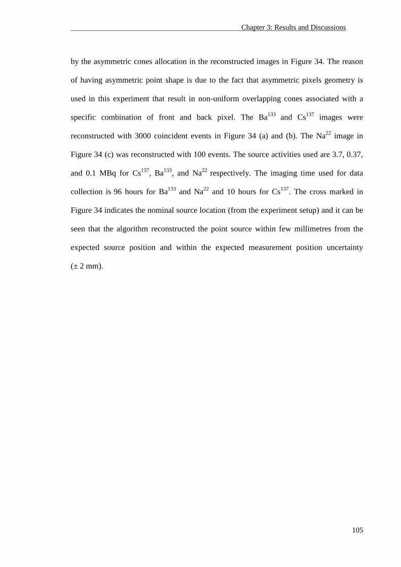
Chapter 3: Results and Discussions
105
by the asymmetric cones allocation in the reconstructed images in Figure 34. The reason
of having asymmetric point shape is due to the fact that asymmetric pixels geometry is
used in this experiment that result in non-uniform overlapping cones associated with a
specific combination of front and back pixel. The Ba133
and Cs137
images were
reconstructed with 3000 coincident events in Figure 34 (a) and (b). The Na22
image in
Figure 34 (c) was reconstructed with 100 events. The source activities used are 3.7, 0.37,
and 0.1 MBq for Cs137
, Ba133
, and Na22
respectively. The imaging time used for data
collection is 96 hours for Ba
133 and Na
22 and 10 hours for Cs
137. The cross marked in
Figure 34 indicates the nominal source location (from the experiment setup) and it can be
seen that the algorithm reconstructed the point source within few millimetres from the
expected source position and within the expected measurement position uncertainty
(± 2 mm).
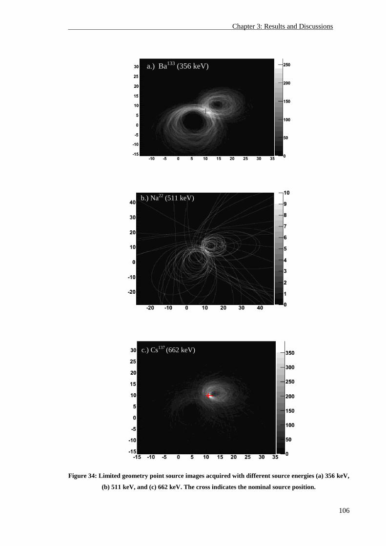
Chapter 3: Results and Discussions
106
Figure 34: Limited geometry point source images acquired with different source energies (a) 356 keV,
(b) 511 keV, and (c) 662 keV. The cross indicates the nominal source position.
a.) Ba133
(356 keV)
b.) Na22
(511 keV)
c.) Cs137
(662 keV)
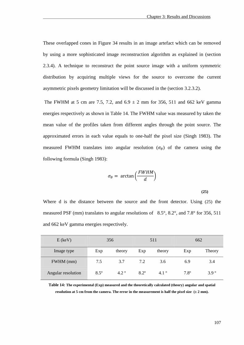
Chapter 3: Results and Discussions
107
These overlapped cones in Figure 34 results in an image artefact which can be removed
by using a more sophisticated image reconstruction algorithm as explained in (section
2.3.4). A technique to reconstruct the point source image with a uniform symmetric
distribution by acquiring multiple views for the source to overcome the current
asymmetric pixels geometry limitation will be discussed in the (section 3.2.3.2).
The FWHM at 5 cm are 7.5, 7.2, and 6.9 ± 2 mm for 356, 511 and 662 keV gamma
energies respectively as shown in Table 14. The FWHM value was measured by taken the
mean value of the profiles taken from different angles through the point source. The
approximated errors in each value equals to one-half the pixel size (Singh 1983). The
measured FWHM translates into angular resolution ( ) of the camera using the
following formula (Singh 1983):
(25)
Where d is the distance between the source and the front detector. Using (25) the
measured PSF (mm) translates to angular resolutions of 8.5°, 8.2°, and 7.8° for 356, 511
and 662 keV gamma energies respectively.
E (keV) 356 511 662
Image type Exp theory Exp theory Exp Theory
FWHM (mm) 7.5 3.7 7.2 3.6 6.9 3.4
Angular resolution 8.5º 4.2 º 8.2º 4.1 º 7.8º 3.9 º
Table 14: The experimental (Exp) measured and the theoretically calculated (theory) angular and spatial
resolution at 5 cm from the camera. The error in the measurement is half the pixel size (± 2 mm).

Chapter 3: Results and Discussions
108
As shown in Table 14 the disagreement between theoretical and experimental values is
due to the fact that the effect of the random events, dead time, and the reconstruction
algorithm decoding penalty were not considered in the theoretical calculation. The
geometry effect resulted in worse than theoretically expected angular resolution as shown
in Table 14. The FWHM values in Table 14 were plotted for different source energies as
shown in Figure 35 .
Figure 35: The experimental measured FWHM (mm) for 356, 511, and 662 keV. The R2 suggests a good fit.
The results in Figure 35 show that the measured spatial resolution is a function of source
energy. However, the inherent system spatial resolution limitation makes the relation
between the spatial resolution and energy invariable at certain point. From the graph
linear equation it can be concluded that the camera resolution at 140 keV gamma energy
is 7.9 mm.
y = -0.002x + 8.1993R² = 0.9999
6
6.5
7
7.5
8
250 350 450 550 650 750
FWH
M(m
m)
energy (keV)
Chapter 3: Results and Discussions
109
3.2.3.2 Multiple views images
The limited-angle views of the projection data are insufficient to correctly reconstruct the
distribution of activity. Limited-angle imaging presented in the previous section induces
image artefacts and produce geometric distortions perpendicular to the direction of the
acquired projections. Therefore, the technique mentioned in (section 2.3.6) was used to
image a Cs137
point from different angles around the camera central axis. The source was
placed 3 cm from the front detector and imaged from 8 different positions as shown in
Figure 36. Then, all the images acquired at different angles were summed together
resulting in an image of cones intersecting from eight different angles at the location of
the point source as shown in Figure 37.
The superimposed summed image provides a more accurate representation for the actual
source distribution as seen in Figure 37 (b). The number of events collected in each
position was 3000 and the final summed image was reconstructed with 24,000
coincidence events. The total acquisition time is 8 days i.e. 24 hours per view. The long
acquisition time is mainly due to the limited number of pixels and slow readout
electronics.
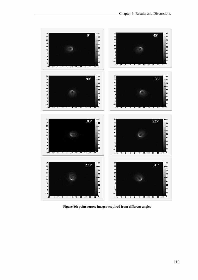
Chapter 3: Results and Discussions
110
Figure 36: point source images acquired from different angles
0° 45°
90° 135°
180° 225°
315° 270°
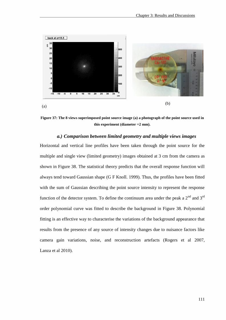
Chapter 3: Results and Discussions
111
(a)
(b)
Figure 37: The 8 views superimposed point source image (a) a photograph of the point source used in
this experiment (diameter =2 mm).
a.) Comparison between limited geometry and multiple views images
Horizontal and vertical line profiles have been taken through the point source for the
multiple and single view (limited geometry) images obtained at 3 cm from the camera as
shown in Figure 38. The statistical theory predicts that the overall response function will
always tend toward Gaussian shape (G F Knoll. 1999). Thus, the profiles have been fitted
with the sum of Gaussian describing the point source intensity to represent the response
function of the detector system. To define the continuum area under the peak a 2nd
and 3rd
order polynomial curve was fitted to describe the background in Figure 38. Polynomial
fitting is an effective way to characterise the variations of the background appearance that
results from the presence of any source of intensity changes due to nuisance factors like
camera gain variations, noise, and reconstruction artefacts (Rogers et al 2007,
Lanza et al 2010).
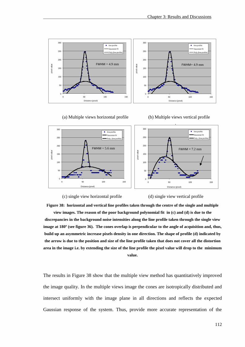
Chapter 3: Results and Discussions
112
(a) Multiple views horizontal profile (b) Multiple views vertical profile
(c) single view horizontal profile (d) single view vertical profile
Figure 38: horizontal and vertical line profiles taken through the centre of the single and multiple
view images. The reason of the poor background polynomial fit in (c) and (d) is due to the
discrepancies in the background noise intensities along the line profile taken through the single view
image at 180º (see figure 36). The cones overlap is perpendicular to the angle of acquisition and, thus,
build up an asymmetric increase pixels density in one direction. The shape of profile (d) indicated by
the arrow is due to the position and size of the line profile taken that does not cover all the distortion
area in the image i.e. by extending the size of the line profile the pixel value will drop to the minimum
value.
The results in Figure 38 show that the multiple view method has quantitatively improved
the image quality. In the multiple views image the cones are isotropically distributed and
intersect uniformly with the image plane in all directions and reflects the expected
Gaussian response of the system. Thus, provide more accurate representation of the
0
50
100
150
200
250
300
0 50 100 150
pix
el v
alu
e
Distance (pixel)
line profile
Gaussian fit
Poly. (line profile)
0
50
100
150
200
250
300
0 50 100 150
pix
el v
alu
e
Distance (pixel)
line profile
Gaussian fit
Poly. (line profile)
0
50
100
150
200
250
300
0 50 100 150
pix
el v
alu
e
Distance (pixel)
line profile
Gaussian fit
Poly.(line profile)
0
50
100
150
200
250
300
0 50 100 150
pix
el v
alu
e
Distance (pixel)
line profile
Gaussian fit
Poly.(line profile)
FWHM = 5.6 mm FWHM = 7.2 mm
FWHM= 4.9 mm
FWHM = 4.9 mm
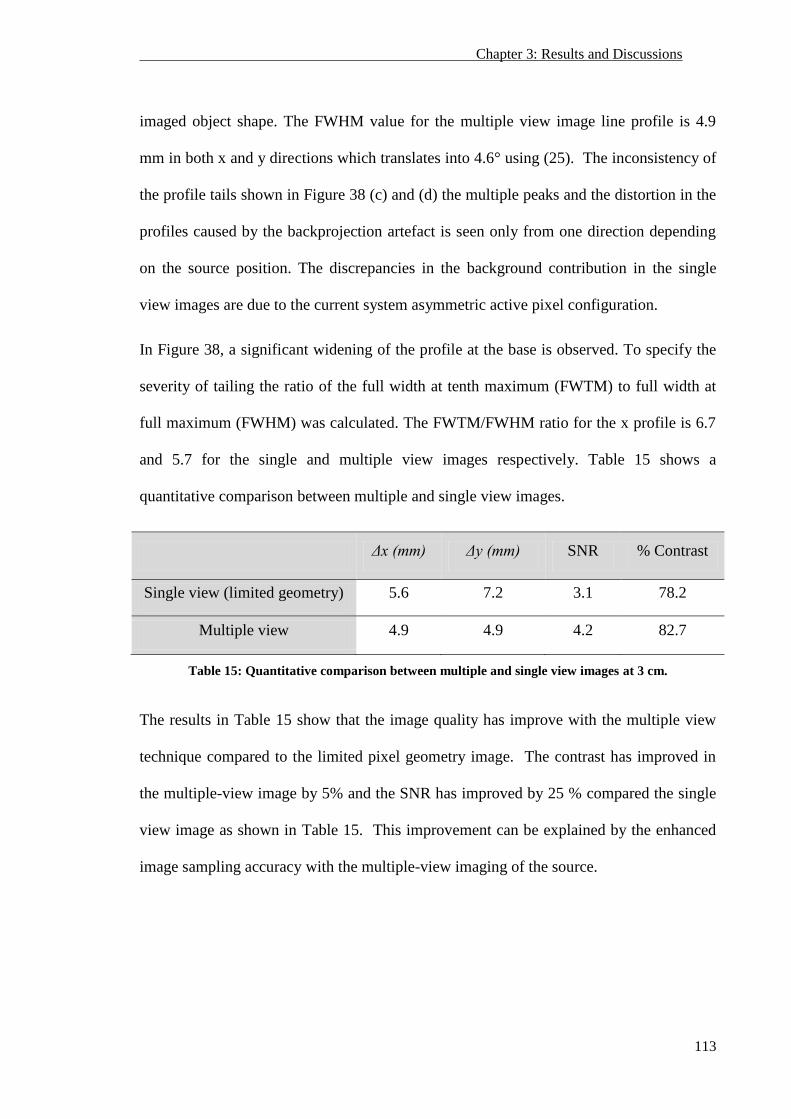
Chapter 3: Results and Discussions
113
imaged object shape. The FWHM value for the multiple view image line profile is 4.9
mm in both x and y directions which translates into 4.6° using (25). The inconsistency of
the profile tails shown in Figure 38 (c) and (d) the multiple peaks and the distortion in the
profiles caused by the backprojection artefact is seen only from one direction depending
on the source position. The discrepancies in the background contribution in the single
view images are due to the current system asymmetric active pixel configuration.
In Figure 38, a significant widening of the profile at the base is observed. To specify the
severity of tailing the ratio of the full width at tenth maximum (FWTM) to full width at
full maximum (FWHM) was calculated. The FWTM/FWHM ratio for the x profile is 6.7
and 5.7 for the single and multiple view images respectively. Table 15 shows a
quantitative comparison between multiple and single view images.
Δx (mm) Δy (mm) SNR % Contrast
Single view (limited geometry) 5.6 7.2 3.1 78.2
Multiple view 4.9 4.9 4.2 82.7
Table 15: Quantitative comparison between multiple and single view images at 3 cm.
The results in Table 15 show that the image quality has improve with the multiple view
technique compared to the limited pixel geometry image. The contrast has improved in
the multiple-view image by 5% and the SNR has improved by 25 % compared the single
view image as shown in Table 15. This improvement can be explained by the enhanced
image sampling accuracy with the multiple-view imaging of the source.
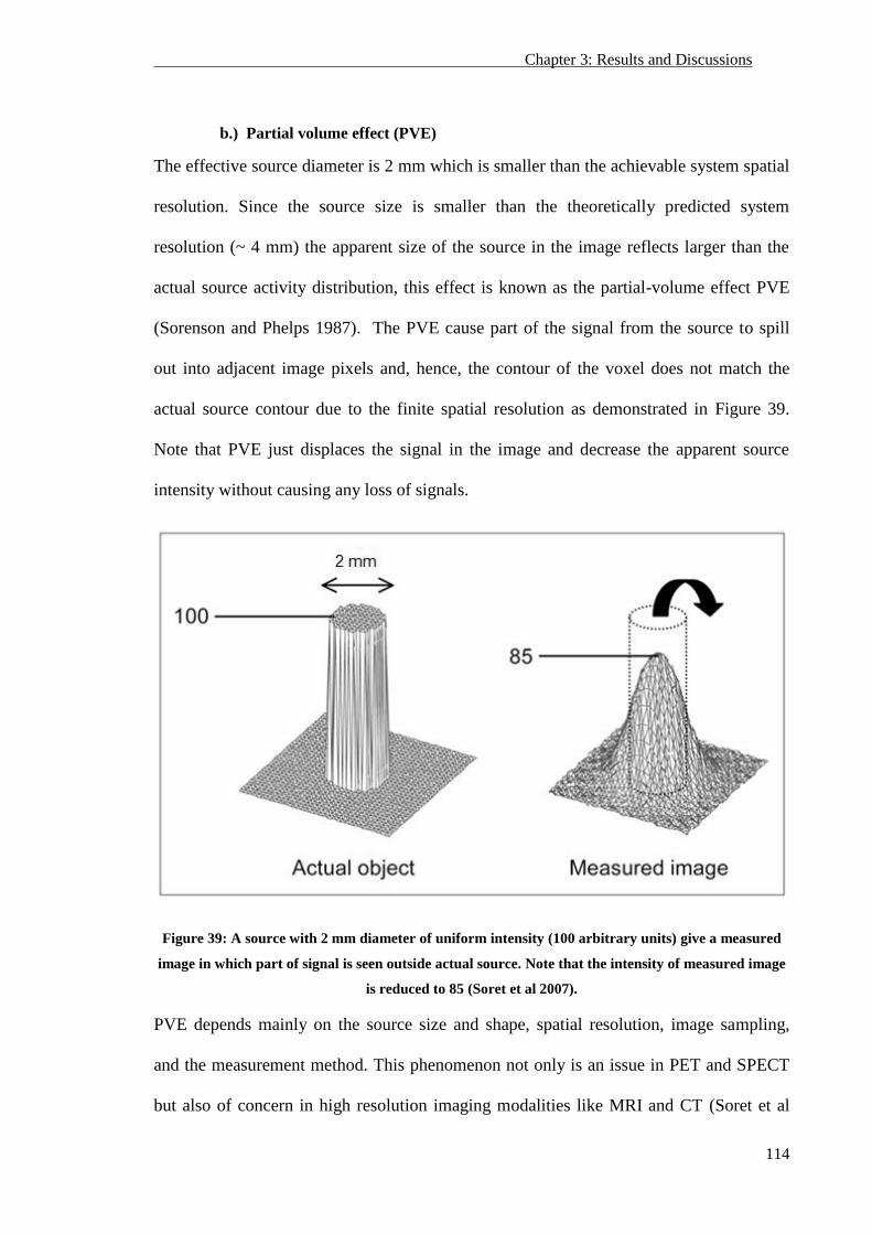
Chapter 3: Results and Discussions
114
b.) Partial volume effect (PVE)
The effective source diameter is 2 mm which is smaller than the achievable system spatial
resolution. Since the source size is smaller than the theoretically predicted system
resolution (~ 4 mm) the apparent size of the source in the image reflects larger than the
actual source activity distribution, this effect is known as the partial-volume effect PVE
(Sorenson and Phelps 1987). The PVE cause part of the signal from the source to spill
out into adjacent image pixels and, hence, the contour of the voxel does not match the
actual source contour due to the finite spatial resolution as demonstrated in Figure 39.
Note that PVE just displaces the signal in the image and decrease the apparent source
intensity without causing any loss of signals.
Figure 39: A source with 2 mm diameter of uniform intensity (100 arbitrary units) give a measured
image in which part of signal is seen outside actual source. Note that the intensity of measured image
is reduced to 85 (Soret et al 2007).
PVE depends mainly on the source size and shape, spatial resolution, image sampling,
and the measurement method. This phenomenon not only is an issue in PET and SPECT
but also of concern in high resolution imaging modalities like MRI and CT (Soret et al
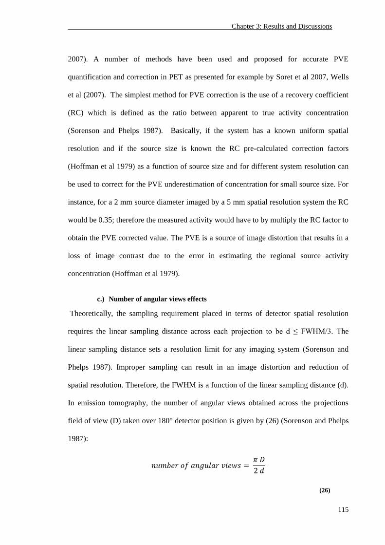
Chapter 3: Results and Discussions
115
2007). A number of methods have been used and proposed for accurate PVE
quantification and correction in PET as presented for example by Soret et al 2007, Wells
et al (2007). The simplest method for PVE correction is the use of a recovery coefficient
(RC) which is defined as the ratio between apparent to true activity concentration
(Sorenson and Phelps 1987). Basically, if the system has a known uniform spatial
resolution and if the source size is known the RC pre-calculated correction factors
(Hoffman et al 1979) as a function of source size and for different system resolution can
be used to correct for the PVE underestimation of concentration for small source size. For
instance, for a 2 mm source diameter imaged by a 5 mm spatial resolution system the RC
would be 0.35; therefore the measured activity would have to by multiply the RC factor to
obtain the PVE corrected value. The PVE is a source of image distortion that results in a
loss of image contrast due to the error in estimating the regional source activity
concentration (Hoffman et al 1979).
c.) Number of angular views effects
Theoretically, the sampling requirement placed in terms of detector spatial resolution
requires the linear sampling distance across each projection to be d ≤ FWHM/3. The
linear sampling distance sets a resolution limit for any imaging system (Sorenson and
Phelps 1987). Improper sampling can result in an image distortion and reduction of
spatial resolution. Therefore, the FWHM is a function of the linear sampling distance (d).
In emission tomography, the number of angular views obtained across the projections
field of view (D) taken over 180° detector position is given by (26) (Sorenson and Phelps
1987):
(26)
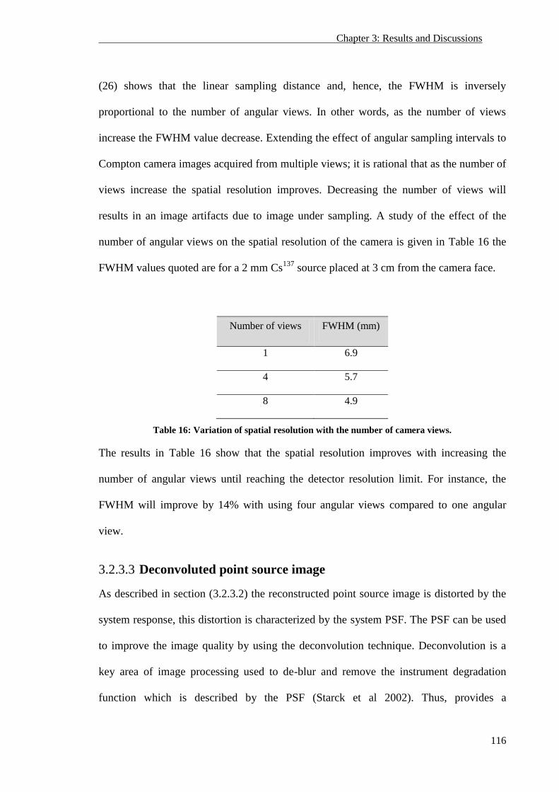
Chapter 3: Results and Discussions
116
(26) shows that the linear sampling distance and, hence, the FWHM is inversely
proportional to the number of angular views. In other words, as the number of views
increase the FWHM value decrease. Extending the effect of angular sampling intervals to
Compton camera images acquired from multiple views; it is rational that as the number of
views increase the spatial resolution improves. Decreasing the number of views will
results in an image artifacts due to image under sampling. A study of the effect of the
number of angular views on the spatial resolution of the camera is given in Table 16 the
FWHM values quoted are for a 2 mm Cs137
source placed at 3 cm from the camera face.
Number of views FWHM (mm)
1 6.9
4 5.7
8 4.9
Table 16: Variation of spatial resolution with the number of camera views.
The results in Table 16 show that the spatial resolution improves with increasing the
number of angular views until reaching the detector resolution limit. For instance, the
FWHM will improve by 14% with using four angular views compared to one angular
view.
3.2.3.3 Deconvoluted point source image
As described in section ( 3.2.3.2) the reconstructed point source image is distorted by the
system response, this distortion is characterized by the system PSF. The PSF can be used
to improve the image quality by using the deconvolution technique. Deconvolution is a
key area of image processing used to de-blur and remove the instrument degradation
function which is described by the PSF (Starck et al 2002). Thus, provides a
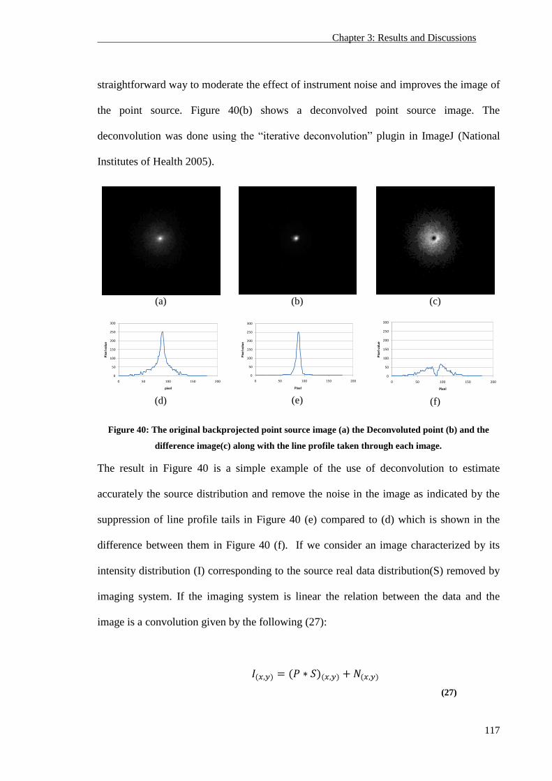
Chapter 3: Results and Discussions
117
straightforward way to moderate the effect of instrument noise and improves the image of
the point source. Figure 40(b) shows a deconvolved point source image. The
deconvolution was done using the “iterative deconvolution” plugin in ImageJ (National
Institutes of Health 2005).
(a) (b) (c)
(d) (e) (f)
Figure 40: The original backprojected point source image (a) the Deconvoluted point (b) and the
difference image(c) along with the line profile taken through each image.
The result in Figure 40 is a simple example of the use of deconvolution to estimate
accurately the source distribution and remove the noise in the image as indicated by the
suppression of line profile tails in Figure 40 (e) compared to (d) which is shown in the
difference between them in Figure 40 (f). If we consider an image characterized by its
intensity distribution (I) corresponding to the source real data distribution(S) removed by
imaging system. If the imaging system is linear the relation between the data and the
image is a convolution given by the following (27):
(27)
0
50
100
150
200
250
300
0 50 100 150 200
Pix
el v
alu
e
pixel
0
50
100
150
200
250
300
0 50 100 150 200
Pix
el v
alu
e
Pixel
0
50
100
150
200
250
300
0 50 100 150 200P
ixe
l val
ue
Pixel
Chapter 3: Results and Discussions
118
Where P is the point spread function and N is the additive system noise. From (27), if
I and P are known the real source distribution S(x,y) can be determined by solving the
inverse problem i.e. deconvolution. This method was used successfully in astronomical
and nuclear medicine studies to create better image. For instance, Starck et al (2002) used
the deconvolution technique to extract scientific content from astronomical images. In
addition, Shao and Karp (1991) used a scattering deconvolution method to accurately
estimate the scatter fraction in SPECT images by modelling the scattering point source
function. Further work is needed to implement a deconvolution algorithm to the
reconstructed data for different source distributions by accurately modelling the system
response.
3.2.4 Distance dependence
The spatial resolution of the Compton camera images is a function of the distance
between the source and the front detector and to demonstrate this concept a Cs137
point
source was imaged at different distance from the camera front surface with the same
acquisition time. The image profile FWHM (mm) was measured for each position and the
results is plotted as FWHM (mm) versus distance (cm) from the front detector as seen in
Figure 41. This experiment was carried out with limited pixel geometry.
The linear equation of the Figure 41 can be used to indicate the expected FWHM values at
different distance. The FWHM of the spatial spread ( ) at a distance D from the
front detector is given by (Singh 1983):
(28)
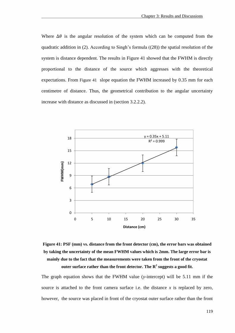
Chapter 3: Results and Discussions
119
Where is the angular resolution of the system which can be computed from the
quadratic addition in (2). According to Singh’s formula ((28)) the spatial resolution of the
system is distance dependent. The results in Figure 41 showed that the FWHM is directly
proportional to the distance of the source which aggresses with the theoretical
expectations. From Figure 41 slope equation the FWHM increased by 0.35 mm for each
centimetre of distance. Thus, the geometrical contribution to the angular uncertainty
increase with distance as discussed in (section 3.2.2.2).
Figure 41: PSF (mm) vs. distance from the front detector (cm), the error bars was obtained
by taking the uncertainty of the mean FWHM values which is 2mm. The large error bar is
mainly due to the fact that the measurements were taken from the front of the cryostat
outer surface rather than the front detector. The R2 suggests a good fit.
The graph equation shows that the FWHM value (y-intercept) will be 5.11 mm if the
source is attached to the front camera surface i.e. the distance x is replaced by zero,
however, the source was placed in front of the cryostat outer surface rather than the front
y = 0.35x + 5.11R² = 0.999
0
3
6
9
12
15
18
0 5 10 15 20 25 30 35
FWH
M(m
m)
Distance (cm)
Chapter 3: Results and Discussions
120
detector due to the camera design, thus, the source is actually placed at ~ 13.3 mm from
the camera front detector, see figure 9 in page 56, adding an additional contribution to the
geometrical effect on angular resolution as described by equation 29. Substituting SFWHM
by 5.11 mm and the distance D by 13.3 mm results in an angular uncertainty of 10º.
The results indicate that the blurring effect will increase for deep imaged structure within
the imaged object, for instance if the source is located at 20 cm from the detector the
image FWHM (mm) will be reduced by a factor of 2 compared to a source located at 5
cm. This effect can be compensated by directly incorporate it in the reconstruction
algorithm as mentioned by Tashiro et al. (2010) which presented a technique to
compensate for this effect with SPECT images. This technique can accurately compensate
for the distance-dependent detector response. By modelling the detector point spread
function as a 2D Gaussian function whose width is dependent on the source-to-detector
distance, a spatially variant inverse filter can be computed and applied to the set of all
sinogram slices.
3.2.5 Efficiency
The efficiency of Compton camera was determined by dividing the number of events
selected as coincidence (useful events) by the number of photons emitted from the source.
For a 3.7 MBq (Cs137
) point source placed at 5 cm from the camera front surface. The
number of coincident events collected ~ 15,500 events which were acquired over 15
hours. This can be translated 0.27 events per second. In addition, the number of 662 keV
gamma-ray photons emitted by Cs137
which is 0.935 was taken into consideration. Thus,
the intrinsic efficiency of Compton camera is the absolute efficiency multiplied by the
geometry factor as calculated from the following formula (J. B Martin et al 1993):
Chapter 3: Results and Discussions
121
(29)
Where Ω is the solid angle calculated by dividing the detector surface area by the source
to detector distance squared) subtended by the front detector which is limited to 0.5
sterradian in the current camera limited pixel geometry. The measured intrinsic efficiency
of the camera with the current limited pixel geometry is 3.0x10⁻¹⁰
for 662 keV source
energy.
The detection efficiency for the experimental measured efficiency is lower than
theoretically estimated efficiency (in section 2.9.2) by four orders of magnitude due to the
limited number of pixels (31 pixels) currently read out. Possible other reasons of this
large difference are the poor triggering performance, data filtering and reconstruction
decoding penalty, timing resolution issues, and the dead time effects which were not
taken into account in the theoretically estimated efficiency.
3.2.6 Timing properties
3.2.6.1 Time resolution
In any timing measurement the generation of a logic pulse that indicates the occurrence
time of an input pulse always involve some degree of uncertainty (Knoll 1999). This
timing inaccuracy can be divided into two categories: random fluctuations in the signal
pulse size and shape which is called time jitter and amplitude walk which is derived
mainly from the variable amplitude of input pulses. The overall timing uncertainty in the
measurement system can be estimated by measuring the full width at half maximum
(FWHM) of the time distribution which is called the time resolution (Knoll 1999). The
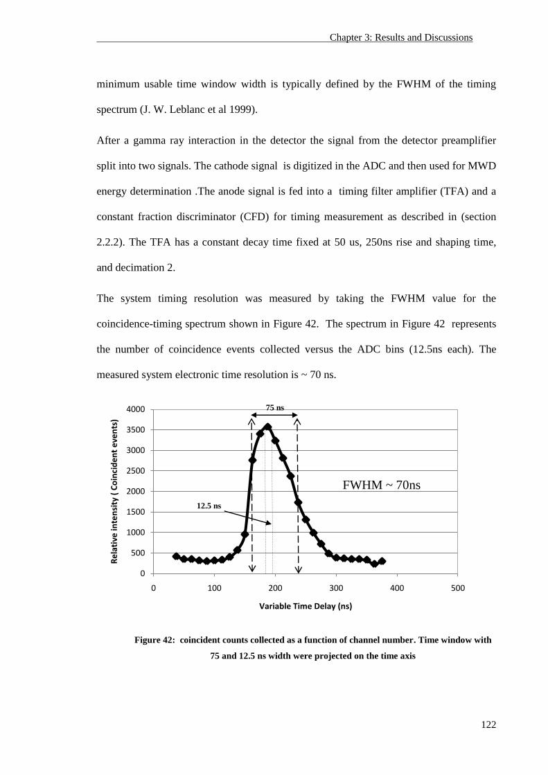
Chapter 3: Results and Discussions
122
minimum usable time window width is typically defined by the FWHM of the timing
spectrum (J. W. Leblanc et al 1999).
After a gamma ray interaction in the detector the signal from the detector preamplifier
split into two signals. The cathode signal is digitized in the ADC and then used for MWD
energy determination .The anode signal is fed into a timing filter amplifier (TFA) and a
constant fraction discriminator (CFD) for timing measurement as described in (section
2.2.2). The TFA has a constant decay time fixed at 50 us, 250ns rise and shaping time,
and decimation 2.
The system timing resolution was measured by taking the FWHM value for the
coincidence-timing spectrum shown in Figure 42. The spectrum in Figure 42 represents
the number of coincidence events collected versus the ADC bins (12.5ns each). The
measured system electronic time resolution is ~ 70 ns.
Figure 42: coincident counts collected as a function of channel number. Time window with
75 and 12.5 ns width were projected on the time axis
0
500
1000
1500
2000
2500
3000
3500
4000
0 100 200 300 400 500
Re
lati
ve in
ten
sity
( C
oin
cid
en
t e
ven
ts)
Variable Time Delay (ns)
FWHM ~ 70ns
75 ns
12.5 ns
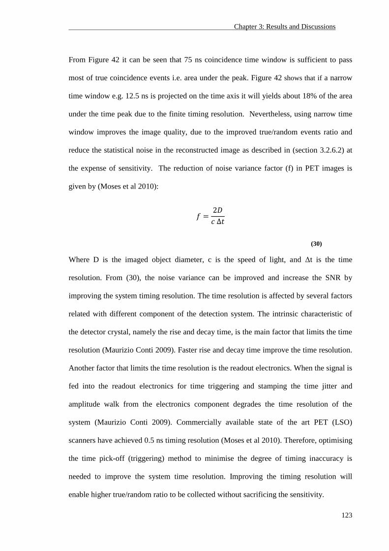
Chapter 3: Results and Discussions
123
From Figure 42 it can be seen that 75 ns coincidence time window is sufficient to pass
most of true coincidence events i.e. area under the peak. Figure 42 shows that if a narrow
time window e.g. 12.5 ns is projected on the time axis it will yields about 18% of the area
under the time peak due to the finite timing resolution. Nevertheless, using narrow time
window improves the image quality, due to the improved true/random events ratio and
reduce the statistical noise in the reconstructed image as described in (section 3.2.6.2) at
the expense of sensitivity. The reduction of noise variance factor (f) in PET images is
given by (Moses et al 2010):
(30)
Where D is the imaged object diameter, c is the speed of light, and Δt is the time
resolution. From (30), the noise variance can be improved and increase the SNR by
improving the system timing resolution. The time resolution is affected by several factors
related with different component of the detection system. The intrinsic characteristic of
the detector crystal, namely the rise and decay time, is the main factor that limits the time
resolution (Maurizio Conti 2009). Faster rise and decay time improve the time resolution.
Another factor that limits the time resolution is the readout electronics. When the signal is
fed into the readout electronics for time triggering and stamping the time jitter and
amplitude walk from the electronics component degrades the time resolution of the
system (Maurizio Conti 2009). Commercially available state of the art PET (LSO)
scanners have achieved 0.5 ns timing resolution (Moses et al 2010). Therefore, optimising
the time pick-off (triggering) method to minimise the degree of timing inaccuracy is
needed to improve the system time resolution. Improving the timing resolution will
enable higher true/random ratio to be collected without sacrificing the sensitivity.
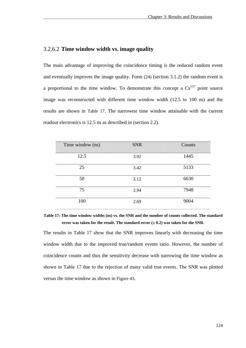
Chapter 3: Results and Discussions
124
3.2.6.2 Time window width vs. image quality
The main advantage of improving the coincidence timing is the reduced random event
and eventually improves the image quality. Form (24) (section 3.1.2) the random event is
a proportional to the time window. To demonstrate this concept a Cs137
point source
image was reconstructed with different time window width (12.5 to 100 ns) and the
results are shown in Table 17. The narrowest time window attainable with the current
readout electronics is 12.5 ns as described in (section 2.2).
Table 17: The time window widths (ns) vs. the SNR and the number of counts collected. The standard
error was taken for the result. The standard error (± 0.2) was taken for the SNR.
The results in Table 17 show that the SNR improves linearly with decreasing the time
window width due to the improved true/random events ratio. However, the number of
coincidence counts and thus the sensitivity decrease with narrowing the time window as
shown in Table 17 due to the rejection of many valid true events. The SNR was plotted
versus the time window as shown in Figure 43.
Time window (ns) SNR Counts
12.5 3.92 1445
25 3.42 5133
50 3.12 6630
75 2.94 7948
100 2.69 9004
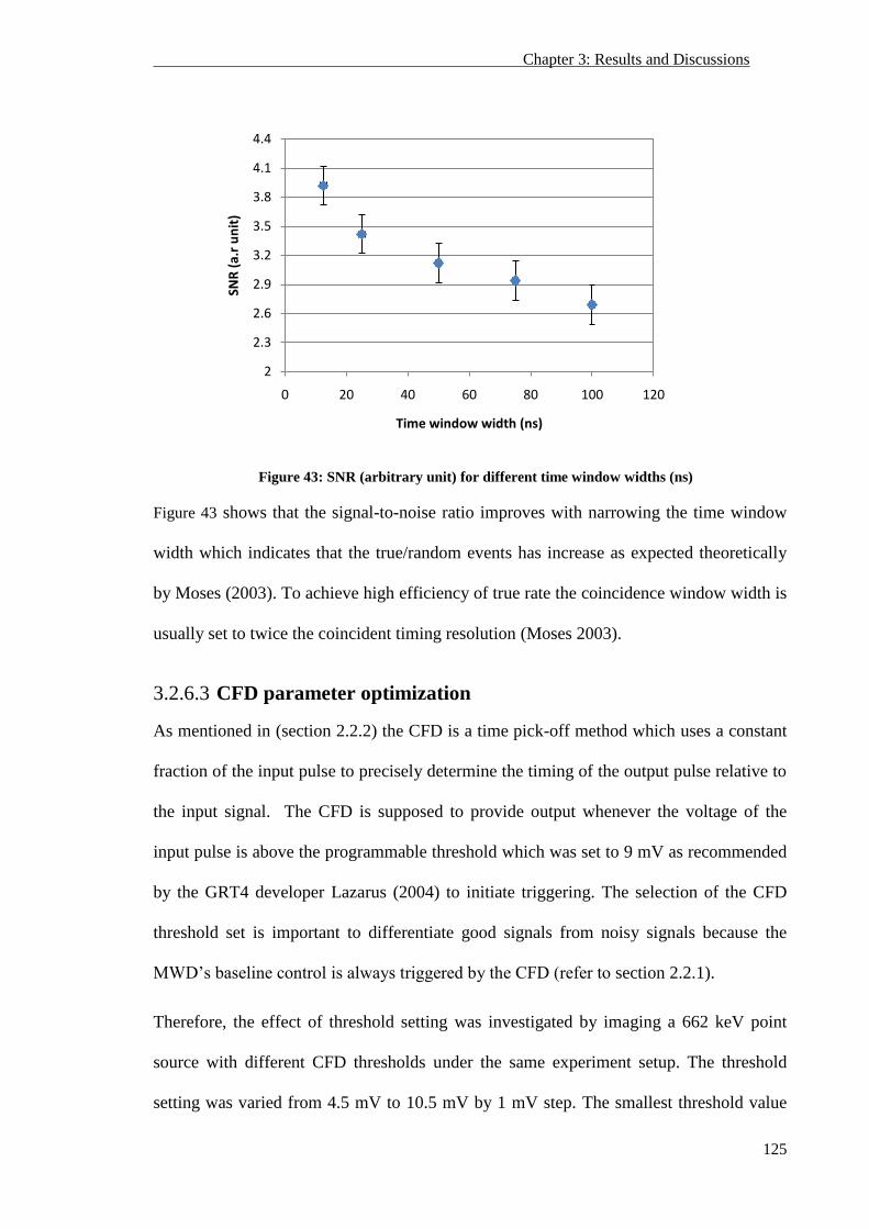
Chapter 3: Results and Discussions
125
Figure 43: SNR (arbitrary unit) for different time window widths (ns)
Figure 43 shows that the signal-to-noise ratio improves with narrowing the time window
width which indicates that the true/random events has increase as expected theoretically
by Moses (2003). To achieve high efficiency of true rate the coincidence window width is
usually set to twice the coincident timing resolution (Moses 2003).
3.2.6.3 CFD parameter optimization
As mentioned in (section 2.2.2) the CFD is a time pick-off method which uses a constant
fraction of the input pulse to precisely determine the timing of the output pulse relative to
the input signal. The CFD is supposed to provide output whenever the voltage of the
input pulse is above the programmable threshold which was set to 9 mV as recommended
by the GRT4 developer Lazarus (2004) to initiate triggering. The selection of the CFD
threshold set is important to differentiate good signals from noisy signals because the
MWD’s baseline control is always triggered by the CFD (refer to section 2.2.1).
Therefore, the effect of threshold setting was investigated by imaging a 662 keV point
source with different CFD thresholds under the same experiment setup. The threshold
setting was varied from 4.5 mV to 10.5 mV by 1 mV step. The smallest threshold value
2
2.3
2.6
2.9
3.2
3.5
3.8
4.1
4.4
0 20 40 60 80 100 120
SNR
(a.
r u
nit
)
Time window width (ns)
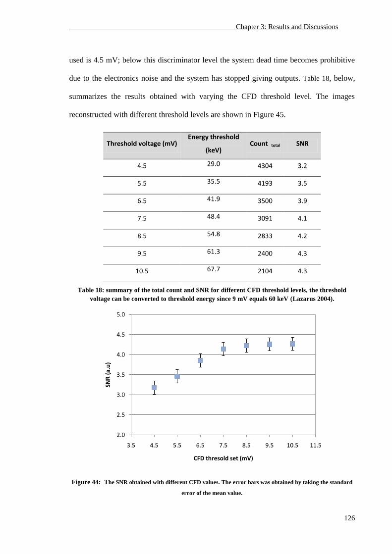
Chapter 3: Results and Discussions
126
used is 4.5 mV; below this discriminator level the system dead time becomes prohibitive
due to the electronics noise and the system has stopped giving outputs. Table 18, below,
summarizes the results obtained with varying the CFD threshold level. The images
reconstructed with different threshold levels are shown in Figure 45.
Threshold voltage (mV) Energy threshold
(keV) Count total SNR
4.5 29.0 4304 3.2
5.5 35.5 4193 3.5
6.5 41.9 3500 3.9
7.5 48.4 3091 4.1
8.5 54.8 2833 4.2
9.5 61.3 2400 4.3
10.5 67.7 2104 4.3
Table 18: summary of the total count and SNR for different CFD threshold levels, the threshold
voltage can be converted to threshold energy since 9 mV equals 60 keV (Lazarus 2004).
Figure 44: The SNR obtained with different CFD values. The error bars was obtained by taking the standard
error of the mean value.
2.0
2.5
3.0
3.5
4.0
4.5
5.0
3.5 4.5 5.5 6.5 7.5 8.5 9.5 10.5 11.5
SNR
(a.
u)
CFD thresold set (mV)
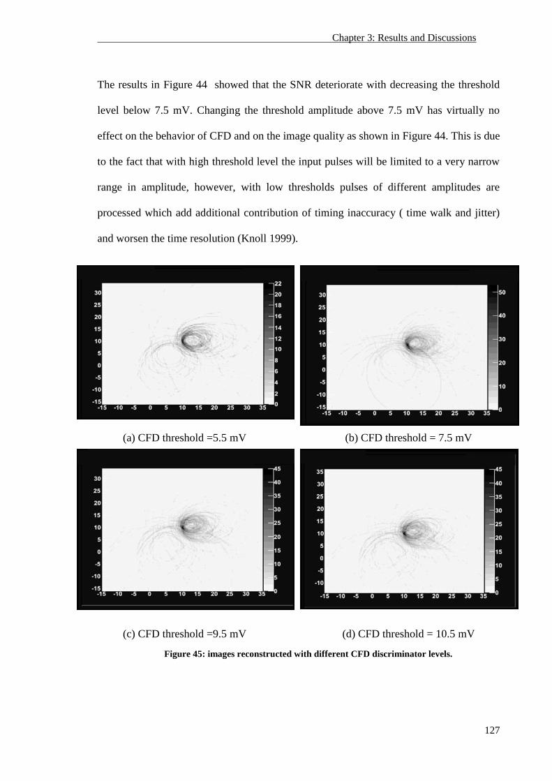
Chapter 3: Results and Discussions
127
The results in Figure 44 showed that the SNR deteriorate with decreasing the threshold
level below 7.5 mV. Changing the threshold amplitude above 7.5 mV has virtually no
effect on the behavior of CFD and on the image quality as shown in Figure 44. This is due
to the fact that with high threshold level the input pulses will be limited to a very narrow
range in amplitude, however, with low thresholds pulses of different amplitudes are
processed which add additional contribution of timing inaccuracy ( time walk and jitter)
and worsen the time resolution (Knoll 1999).
(a) CFD threshold =5.5 mV (b) CFD threshold = 7.5 mV
(c) CFD threshold =9.5 mV (d) CFD threshold = 10.5 mV
Figure 45: images reconstructed with different CFD discriminator levels.
Chapter 3: Results and Discussions
128
As can be seen in Figure 45 (a) and (b) that the images acquired with low CFD threshold
value have a distorted point source shape which is explained by the increase background,
noise. This is because at small threshold level the CFD is not able to discriminate between
low amplitude genuine and background pulses (Knoll 1999).
Whereas, using higher CFD threshold levels as in Figure 45 (c) and (d) clears the images
from background noise, but, at the expense of sensitivity as shown the reduction of the
total counts collected with increasing threshold level in Table 18. The degradation of
image quality with low thresholds is mainly due to the statistical fluctuations in the
number of charge carriers that makes up the signal which is greater for small amplitude
pulses. Therefore, setting the threshold to 7.5mV can compromise between the sensitivity
and image quality.
3.2.7 Counting limitation
The count rate performance of the system is limited by the relatively slow readout
electronics as reflected by the poor timing resolution discussed in (section 3.2.6.1). Under
high incident photons flux or with increasing the number of active pixels bottle neck
behaviour in the data output pipe was observed as will be discussed in the following
paragraphs.
Since the MIDAS data acquisition software does not provide the experiment count rate to
the user, the data transfer rate (DTR) which is the speed at which the acquired data is
transmitted to the data storage tape was used instead as an indicator of the counting
performance.
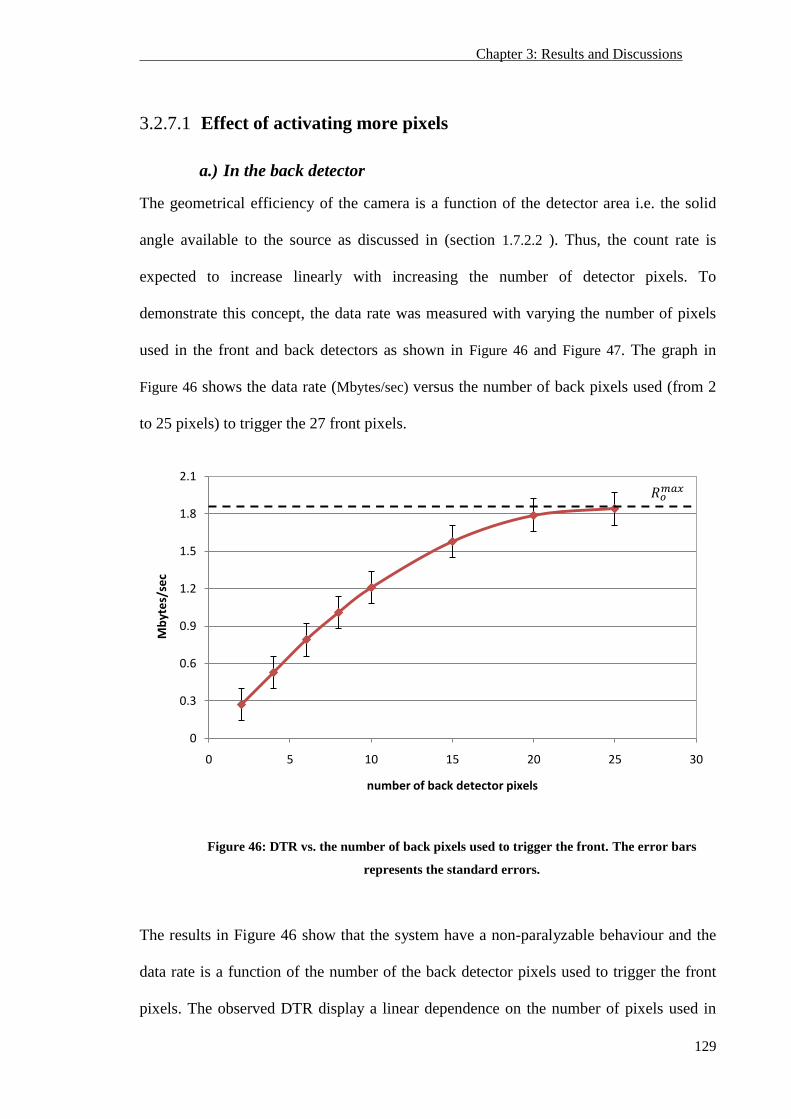
Chapter 3: Results and Discussions
129
3.2.7.1 Effect of activating more pixels
a.) In the back detector
The geometrical efficiency of the camera is a function of the detector area i.e. the solid
angle available to the source as discussed in (section 1.7.2.2 ). Thus, the count rate is
expected to increase linearly with increasing the number of detector pixels. To
demonstrate this concept, the data rate was measured with varying the number of pixels
used in the front and back detectors as shown in Figure 46 and Figure 47. The graph in
Figure 46 shows the data rate (Mbytes/sec) versus the number of back pixels used (from 2
to 25 pixels) to trigger the 27 front pixels.
Figure 46: DTR vs. the number of back pixels used to trigger the front. The error bars
represents the standard errors.
The results in Figure 46 show that the system have a non-paralyzable behaviour and the
data rate is a function of the number of the back detector pixels used to trigger the front
pixels. The observed DTR display a linear dependence on the number of pixels used in
0
0.3
0.6
0.9
1.2
1.5
1.8
2.1
0 5 10 15 20 25 30
Mb
yte
s/se
c
number of back detector pixels
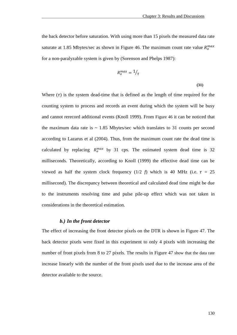
Chapter 3: Results and Discussions
130
the back detector before saturation. With using more than 15 pixels the measured data rate
saturate at 1.85 Mbytes/sec as shown in Figure 46. The maximum count rate value
for a non-paralyzable system is given by (Sorenson and Phelps 1987):
(31)
Where ( ) is the system dead-time that is defined as the length of time required for the
counting system to process and records an event during which the system will be busy
and cannot rerecord additional events (Knoll 1999). From Figure 46 it can be noticed that
the maximum data rate is ~ 1.85 Mbytes/sec which translates to 31 counts per second
according to Lazarus et al (2004). Thus, from the maximum count rate the dead time is
calculated by replacing by 31 cps. The estimated system dead time is 32
milliseconds. Theoretically, according to Knoll (1999) the effective dead time can be
viewed as half the system clock frequency (1/2 f) which is 40 MHz (i.e. = 25
millisecond). The discrepancy between theoretical and calculated dead time might be due
to the instruments resolving time and pulse pile-up effect which was not taken in
considerations in the theoretical estimation.
b.) In the front detector
The effect of increasing the front detector pixels on the DTR is shown in Figure 47. The
back detector pixels were fixed in this experiment to only 4 pixels with increasing the
number of front pixels from 8 to 27 pixels. The results in Figure 47 show that the data rate
increase linearly with the number of the front pixels used due to the increase area of the
detector available to the source.
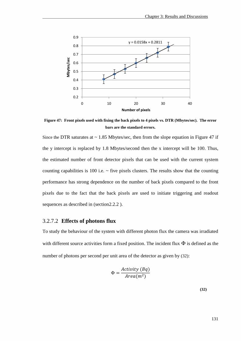
Chapter 3: Results and Discussions
131
Figure 47: Front pixels used with fixing the back pixels to 4 pixels vs. DTR (Mbytes/sec). The error
bars are the standard errors.
Since the DTR saturates at ~ 1.85 Mbytes/sec, then from the slope equation in Figure 47 if
the y intercept is replaced by 1.8 Mbytes/second then the x intercept will be 100. Thus,
the estimated number of front detector pixels that can be used with the current system
counting capabilities is 100 i.e. ~ five pixels clusters. The results show that the counting
performance has strong dependence on the number of back pixels compared to the front
pixels due to the fact that the back pixels are used to initiate triggering and readout
sequences as described in (section 2.2.2 ).
3.2.7.2 Effects of photons flux
To study the behaviour of the system with different photon flux the camera was irradiated
with different source activities form a fixed position. The incident flux is defined as the
number of photons per second per unit area of the detector as given by (32):
(32)
y = 0.0158x + 0.2811
0.2
0.3
0.4
0.5
0.6
0.7
0.8
0.9
0 10 20 30 40
Mb
yte
s/se
c
Number of pixels
Chapter 3: Results and Discussions
132
The activity in Bq is the number of photons/sec and the detector area in meter squared.
The DTR is show in Figure 48 as a function of the incident photon flux. The results show
that the observed DTR display a linear dependence on the incident flux before saturation.
Under strong irradiation (flux > 6x10¹²
photon/sec/m2) the measured data rate again
saturate at ~ 1.85 Mbytes/sec. This indicates that high flux rate result in a multiple
extension of the dead time period following an initial recorded count and the system
hardly has time to finish one dead time period before starting another.
Figure 48: The DTR vs. the incident photons flux. The error bars represents the standard errors.
Figure 48 shows that high photons flux lead to count rate losses due to the system dead
time as described in (section 3.2.7.1 ). Dead time count rate losses are given by the
difference between the observed and true count rate , which is the count rate if =0,
are given by (Sorenson and Phelps 1987):
(33)
0.0
0.3
0.6
0.9
1.2
1.5
1.8
2.1
0.0E+00 2.5E+12 5.0E+12 7.5E+12 1.0E+13 1.3E+13 1.5E+13
DTR
(M
byt
es/
sec)
Flux (photon/sec/m2)
Chapter 3: Results and Discussions
133
Many methods exist for dead-time correction as described by (Sorenson and Phelps 1987,
Kang et al 2008, Chiesa et al 2009) that can be used to compensate for the count rate
losses and improve the counting statistics to provide better quantitative accuracy.
3.3 Distributed source images
Objective and quantitative analysis of the system imaging performance that incorporate
the combined effects of the basic measured system performance as well as the system
processing and the quality of the reconstructed image is presented in this section. In
addition the results of the multiple views imaging technique for line and ring source as
well as a cylindrical phantom are presented in this section.
3.3.1 Cs137
Line source
To test the camera imaging performance with extended source a line source was imaged
at 2 cm from the camera front surface by moving a Cs137
point source into 8 positions
separated by 0.25cm to draw a line shape. The line source image shown in Figure 49 (a)
was reconstructed with 16,000 from limited angle geometry as mentioned in (section 2.1).
Horizontal line profile has been taken through the centre of the line source image as
shown in Figure 49. The FWHM values obtained are 7.2 ± 2mm. The profile distortion
shown in Figure 49(b) is due to the backprojection artefacts which are caused by the
ellipses associated with frequent combination of front and back pixels. The intensity is
not equally distributed due to the geometrical consideration of sensitivity variation at
different source position with the limited area occupied by the detector (Solomon and R J
Ott 1988, Dedek et al 2009).
A correction factor can be applied to the image to compensate for the sensitivity
variations by multiplying the pixels in the low camera sensitivity by 1.25, since there is
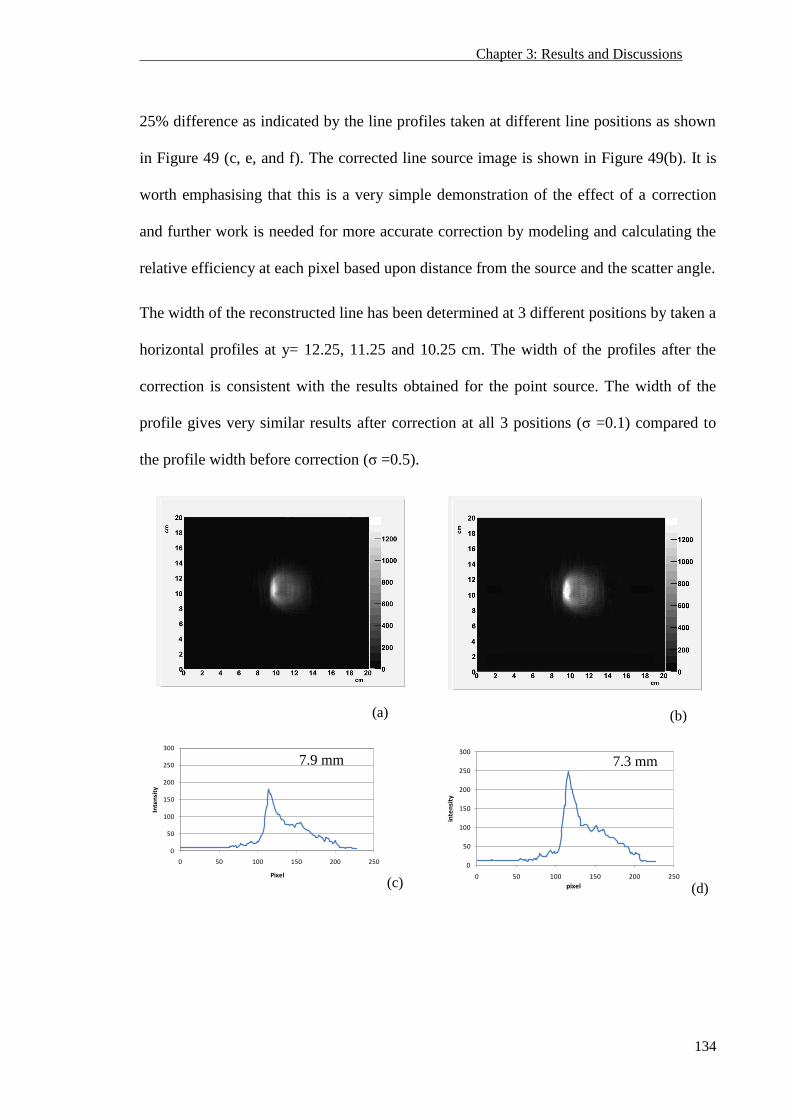
Chapter 3: Results and Discussions
134
25% difference as indicated by the line profiles taken at different line positions as shown
in Figure 49 (c, e, and f). The corrected line source image is shown in Figure 49(b). It is
worth emphasising that this is a very simple demonstration of the effect of a correction
and further work is needed for more accurate correction by modeling and calculating the
relative efficiency at each pixel based upon distance from the source and the scatter angle.
The width of the reconstructed line has been determined at 3 different positions by taken a
horizontal profiles at y= 12.25, 11.25 and 10.25 cm. The width of the profiles after the
correction is consistent with the results obtained for the point source. The width of the
profile gives very similar results after correction at all 3 positions (σ =0.1) compared to
the profile width before correction (σ =0.5).
(a)
(b)
(c) (d)
0
50
100
150
200
250
300
0 50 100 150 200 250
Inte
nsi
ty
Pixel
0
50
100
150
200
250
300
0 50 100 150 200 250
inte
nsi
ty
pixel
7.3 mm 7.9 mm
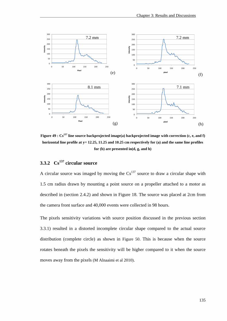
Chapter 3: Results and Discussions
135
(e) (f)
(g) (h)
Figure 49 : Cs137
line source backprojected image(a) backprojected image with correction (c, e, and f)
horizontal line profile at y= 12.25, 11.25 and 10.25 cm respectively for (a) and the same line profiles
for (b) are presented in(d, g, and h)
3.3.2 Cs137
circular source
A circular source was imaged by moving the Cs137
source to draw a circular shape with
1.5 cm radius drawn by mounting a point source on a propeller attached to a motor as
described in (section 2.4.2) and shown in Figure 18. The source was placed at 2cm from
the camera front surface and 40,000 events were collected in 98 hours.
The pixels sensitivity variations with source position discussed in the previous section
3.3.1) resulted in a distorted incomplete circular shape compared to the actual source
distribution (complete circle) as shown in Figure 50. This is because when the source
rotates beneath the pixels the sensitivity will be higher compared to it when the source
moves away from the pixels (M Alnaaimi et al 2010).
0
50
100
150
200
250
300
0 50 100 150 200 250
inte
nsi
ty
Pixel
0
50
100
150
200
250
300
0 50 100 150 200 250
inte
nsi
ty
pixel
0
50
100
150
200
250
300
0 50 100 150 200 250
inte
nsi
ty
Pixel
0
50
100
150
200
250
300
0 50 100 150 200 250
inte
nsi
ty
pixel
7.2 mm
7.1 mm 8.1 mm
7.2 mm
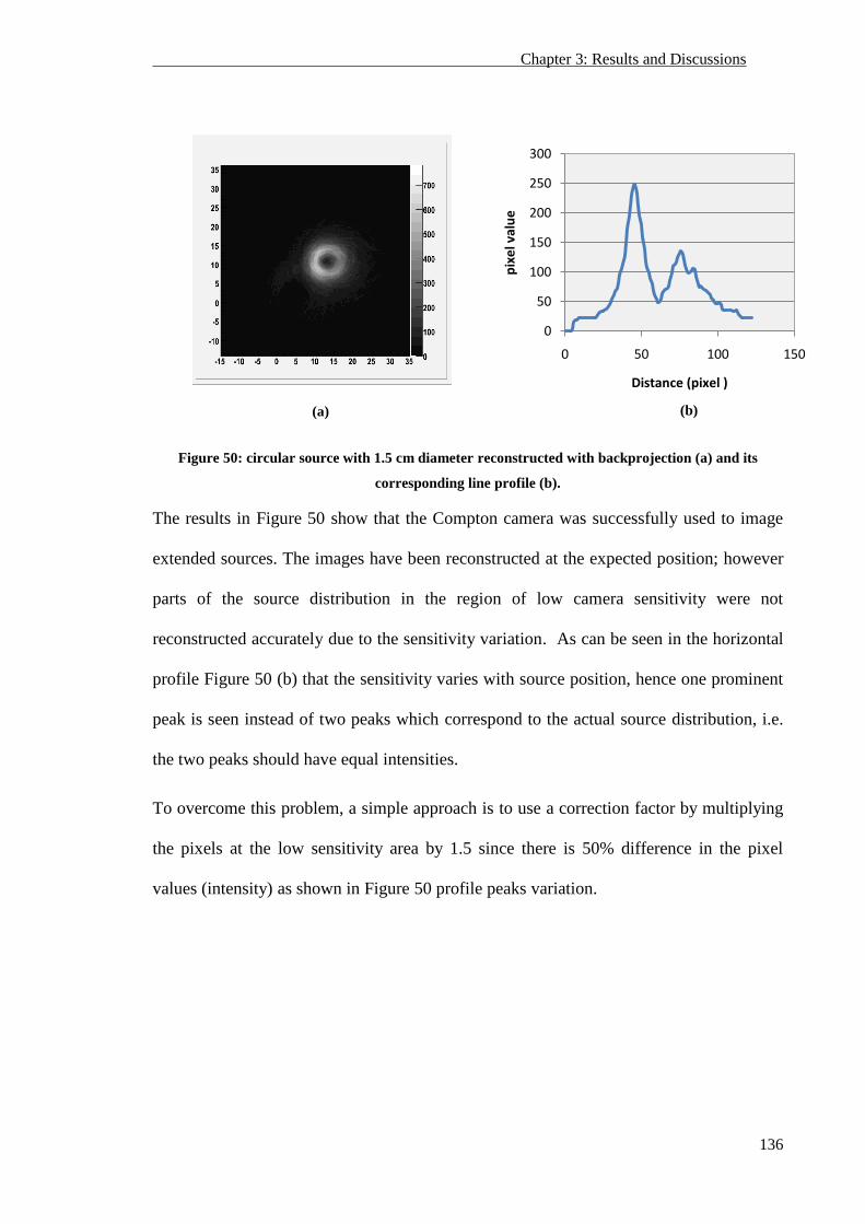
Chapter 3: Results and Discussions
136
(a) (b)
Figure 50: circular source with 1.5 cm diameter reconstructed with backprojection (a) and its
corresponding line profile (b).
The results in Figure 50 show that the Compton camera was successfully used to image
extended sources. The images have been reconstructed at the expected position; however
parts of the source distribution in the region of low camera sensitivity were not
reconstructed accurately due to the sensitivity variation. As can be seen in the horizontal
profile Figure 50 (b) that the sensitivity varies with source position, hence one prominent
peak is seen instead of two peaks which correspond to the actual source distribution, i.e.
the two peaks should have equal intensities.
To overcome this problem, a simple approach is to use a correction factor by multiplying
the pixels at the low sensitivity area by 1.5 since there is 50% difference in the pixel
values (intensity) as shown in Figure 50 profile peaks variation.
0
50
100
150
200
250
300
0 50 100 150
pix
el v
alu
e
Distance (pixel )
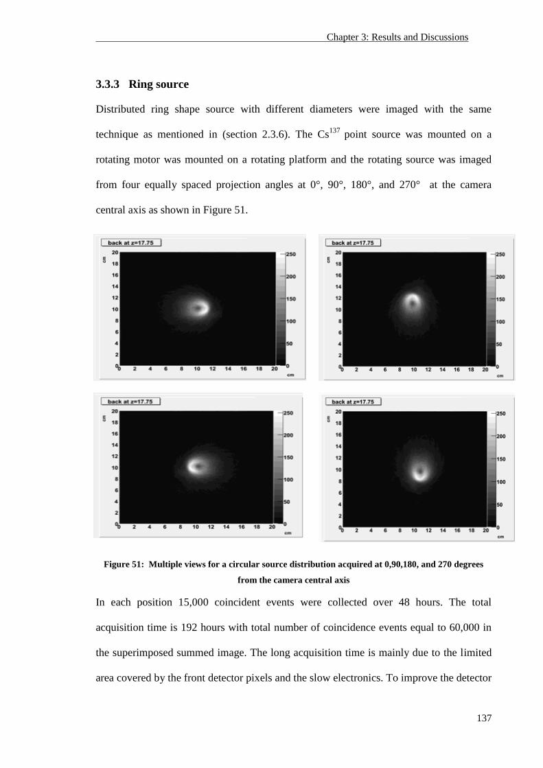
Chapter 3: Results and Discussions
137
3.3.3 Ring source
Distributed ring shape source with different diameters were imaged with the same
technique as mentioned in (section 2.3.6). The Cs137
point source was mounted on a
rotating motor was mounted on a rotating platform and the rotating source was imaged
from four equally spaced projection angles at 0°, 90°, 180°, and 270° at the camera
central axis as shown in Figure 51.
Figure 51: Multiple views for a circular source distribution acquired at 0,90,180, and 270 degrees
from the camera central axis
In each position 15,000 coincident events were collected over 48 hours. The total
acquisition time is 192 hours with total number of coincidence events equal to 60,000 in
the superimposed summed image. The long acquisition time is mainly due to the limited
area covered by the front detector pixels and the slow electronics. To improve the detector
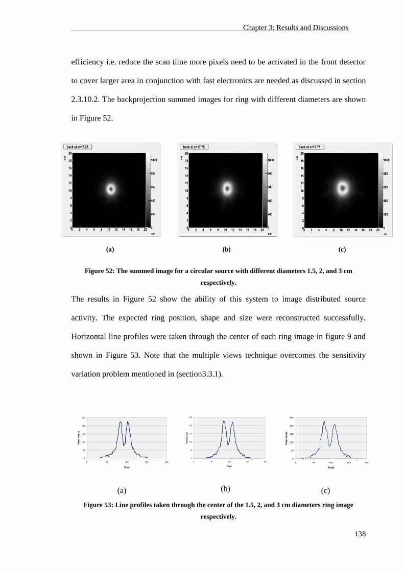
Chapter 3: Results and Discussions
138
efficiency i.e. reduce the scan time more pixels need to be activated in the front detector
to cover larger area in conjunction with fast electronics are needed as discussed in section
2.3.10.2. The backprojection summed images for ring with different diameters are shown
in Figure 52.
(a)
(b)
(c)
Figure 52: The summed image for a circular source with different diameters 1.5, 2, and 3 cm
respectively.
The results in Figure 52 show the ability of this system to image distributed source
activity. The expected ring position, shape and size were reconstructed successfully.
Horizontal line profiles were taken through the center of each ring image in figure 9 and
shown in Figure 53. Note that the multiple views technique overcomes the sensitivity
variation problem mentioned in (section 3.3.1).
(a)
(b)
(c)
Figure 53: Line profiles taken through the center of the 1.5, 2, and 3 cm diameters ring image
respectively.
0
50
100
150
200
250
0 50 100 150 200
Pix
el v
alu
e
Pixel
0
50
100
150
200
250
0 50 100 150 200
Pix
el v
alu
e
Pixel
0
50
100
150
200
250
0 50 100 150 200
Pix
el v
alu
e
Pixel
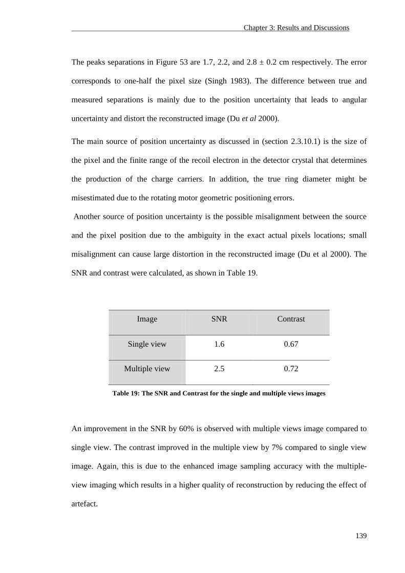
Chapter 3: Results and Discussions
139
The peaks separations in Figure 53 are 1.7, 2.2, and 2.8 ± 0.2 cm respectively. The error
corresponds to one-half the pixel size (Singh 1983). The difference between true and
measured separations is mainly due to the position uncertainty that leads to angular
uncertainty and distort the reconstructed image (Du et al 2000).
The main source of position uncertainty as discussed in (section 2.3.10.1) is the size of
the pixel and the finite range of the recoil electron in the detector crystal that determines
the production of the charge carriers. In addition, the true ring diameter might be
misestimated due to the rotating motor geometric positioning errors.
Another source of position uncertainty is the possible misalignment between the source
and the pixel position due to the ambiguity in the exact actual pixels locations; small
misalignment can cause large distortion in the reconstructed image (Du et al 2000). The
SNR and contrast were calculated, as shown in Table 19.
Image SNR Contrast
Single view 1.6 0.67
Multiple view 2.5 0.72
Table 19: The SNR and Contrast for the single and multiple views images
An improvement in the SNR by 60% is observed with multiple views image compared to
single view. The contrast improved in the multiple view by 7% compared to single view
image. Again, this is due to the enhanced image sampling accuracy with the multiple-
view imaging which results in a higher quality of reconstruction by reducing the effect of
artefact.
Chapter 3: Results and Discussions
140
3.4 Resolving power
The resolving power is the ability of an imaging device to measure the separation
between two adjacent points. This method is a more precise way to measure the FWHM
since the distance between the peaks of two curves from the profile histogram represents
the known distance between the two points. The maximum profile counts (peak)
represents the center of point source and the number of pixels separating the two peaks
would be equivalent to the known distance.
The resolving power of the camera was investigated by imaging two Cs137
point sources
separated by 3.5 mm. The two points are clearly separated and identified as two sources,
as shown in figure 54. This image demonstrates Sorenson and Phelps (1987) assumption
which states that the resolving power should be between FWHM/2 and FWHM/1.4. Since
the FWHM of the system measured for a point source from a multiple view acquisition is
4.9 mm as discussed in (section 3.2.3.2) the resolving power for this system is expected to
be 3.5 mm. In addition, the horizontal line profile taken through the two points showed
two barely distinguishable peaks. The artefact caused by the reconstruction method
resulted in overlapped peaks.
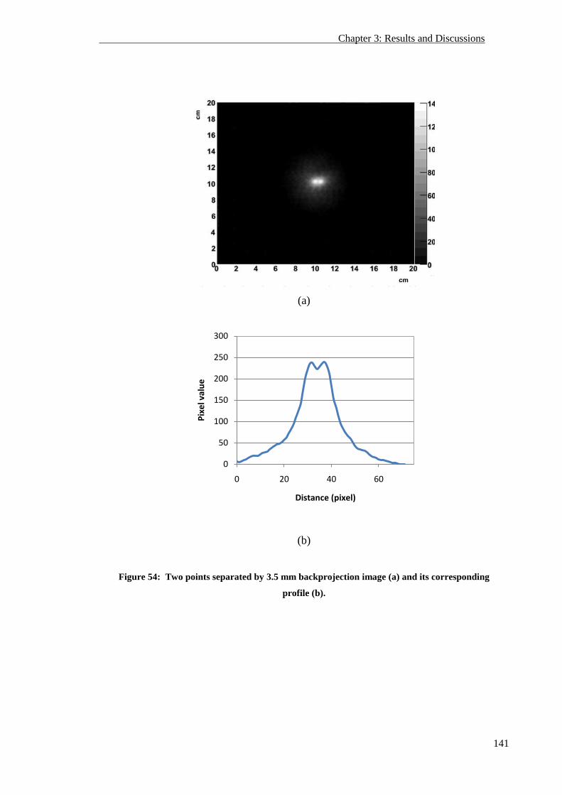
Chapter 3: Results and Discussions
141
(a)
(b)
Figure 54: Two points separated by 3.5 mm backprojection image (a) and its corresponding
profile (b).
0
50
100
150
200
250
300
0 20 40 60
Pix
el v
alu
e
Distance (pixel)
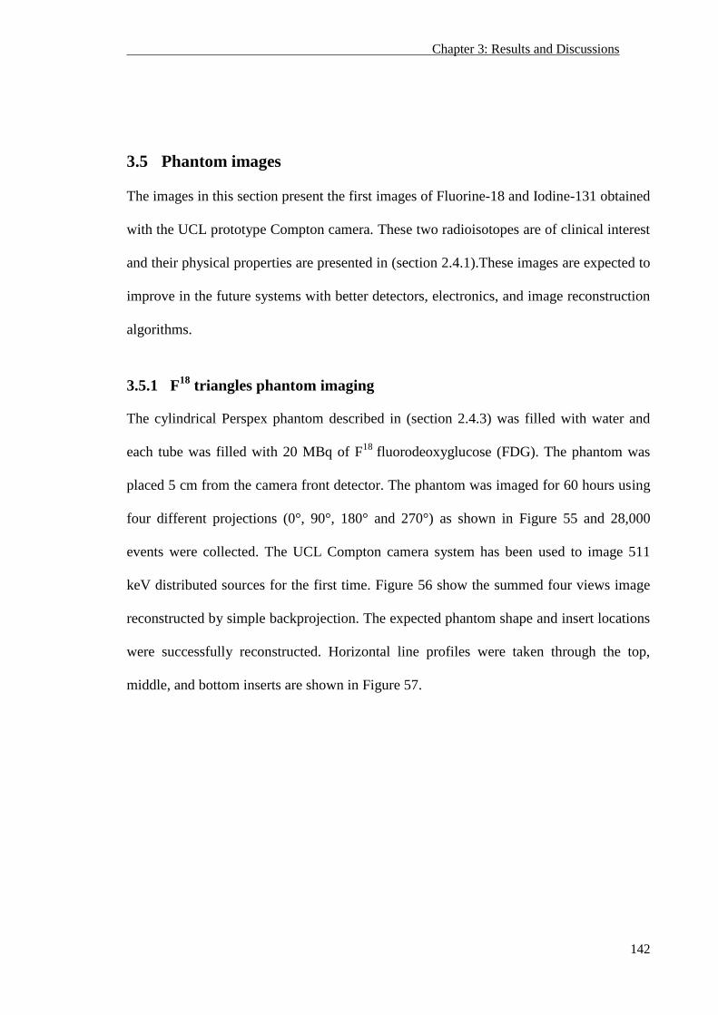
Chapter 3: Results and Discussions
142
3.5 Phantom images
The images in this section present the first images of Fluorine-18 and Iodine-131 obtained
with the UCL prototype Compton camera. These two radioisotopes are of clinical interest
and their physical properties are presented in (section 2.4.1).These images are expected to
improve in the future systems with better detectors, electronics, and image reconstruction
algorithms.
3.5.1 F18
triangles phantom imaging
The cylindrical Perspex phantom described in (section 2.4.3) was filled with water and
each tube was filled with 20 MBq of F18
fluorodeoxyglucose (FDG). The phantom was
placed 5 cm from the camera front detector. The phantom was imaged for 60 hours using
four different projections (0°, 90°, 180° and 270°) as shown in Figure 55 and 28,000
events were collected. The UCL Compton camera system has been used to image 511
keV distributed sources for the first time. Figure 56 show the summed four views image
reconstructed by simple backprojection. The expected phantom shape and insert locations
were successfully reconstructed. Horizontal line profiles were taken through the top,
middle, and bottom inserts are shown in Figure 57.
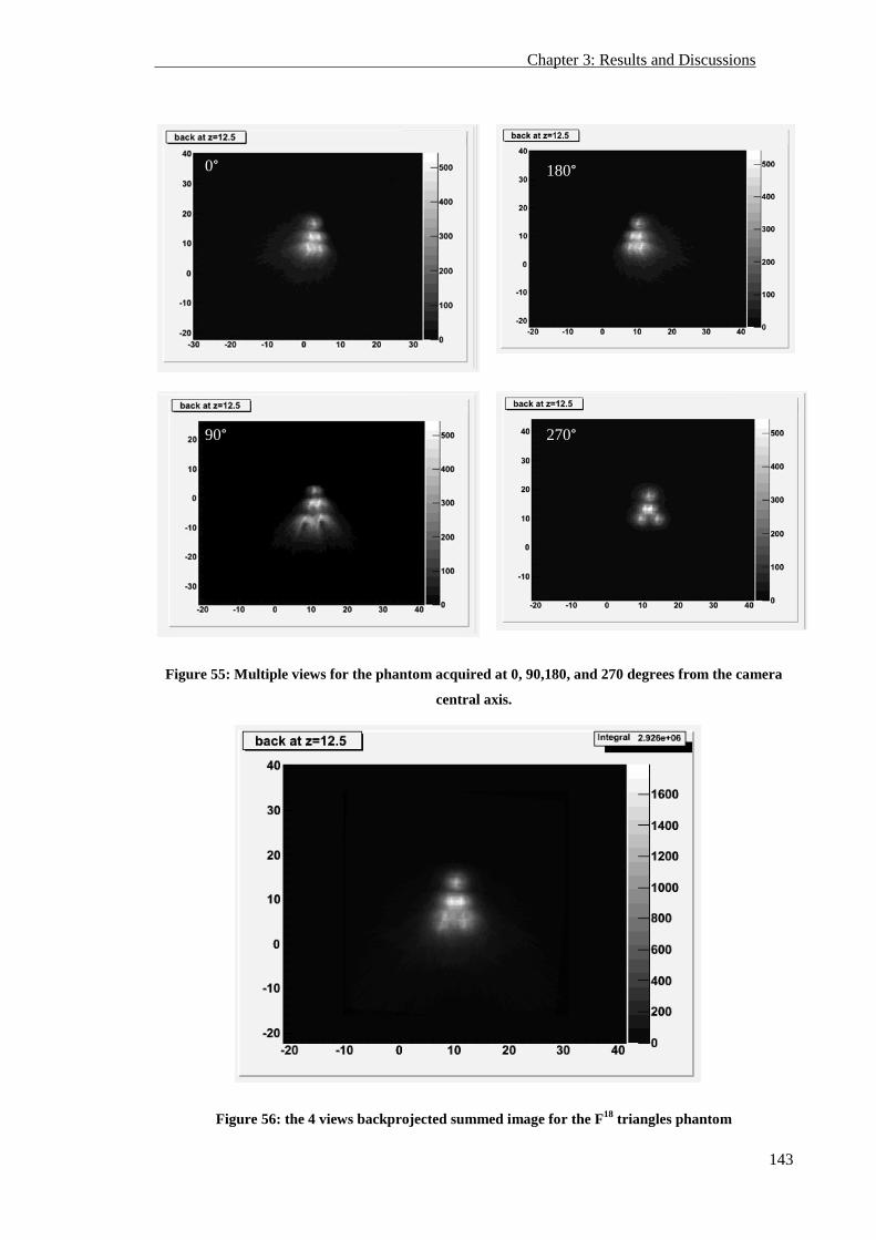
Chapter 3: Results and Discussions
143
Figure 55: Multiple views for the phantom acquired at 0, 90,180, and 270 degrees from the camera
central axis.
Figure 56: the 4 views backprojected summed image for the F18
triangles phantom
0° 180°
90° 270°
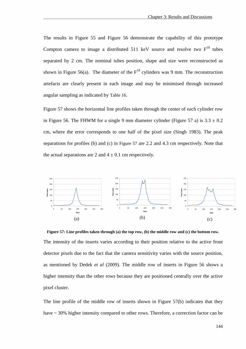
Chapter 3: Results and Discussions
144
The results in Figure 55 and Figure 56 demonstrate the capability of this prototype
Compton camera to image a distributed 511 keV source and resolve two F18
tubes
separated by 2 cm. The nominal tubes position, shape and size were reconstructed as
shown in Figure 56(a). The diameter of the F18
cylinders was 9 mm. The reconstruction
artefacts are clearly present in each image and may be minimised through increased
angular sampling as indicated by Table 16.
Figure 57 shows the horizontal line profiles taken through the center of each cylinder row
in Figure 56. The FHWM for a single 9 mm diameter cylinder (Figure 57 a) is 3.3 ± 0.2
cm, where the error corresponds to one half of the pixel size (Singh 1983). The peak
separations for profiles (b) and (c) in Figure 57 are 2.2 and 4.3 cm respectively. Note that
the actual separations are 2 and 4 ± 0.1 cm respectively.
(a)
(b)
(c)
Figure 57: Line profiles taken through (a) the top row, (b) the middle row and (c) the bottom row.
The intensity of the inserts varies according to their position relative to the active front
detector pixels due to the fact that the camera sensitivity varies with the source position,
as mentioned by Dedek et al (2009). The middle row of inserts in Figure 56 shows a
higher intensity than the other rows because they are positioned centrally over the active
pixel cluster.
The line profile of the middle row of inserts shown in Figure 57(b) indicates that they
have ~ 30% higher intensity compared to other rows. Therefore, a correction factor can be
0
50
100
150
200
250
0 50 100 150 200 250 300
Pix
el v
alu
e
Pixel
0
50
100
150
200
250
0 50 100 150 200 250 300
Pix
el v
alu
e
Pixel
0
50
100
150
200
250
0 50 100 150 200 250 300
Pix
el v
alu
e
Pixel
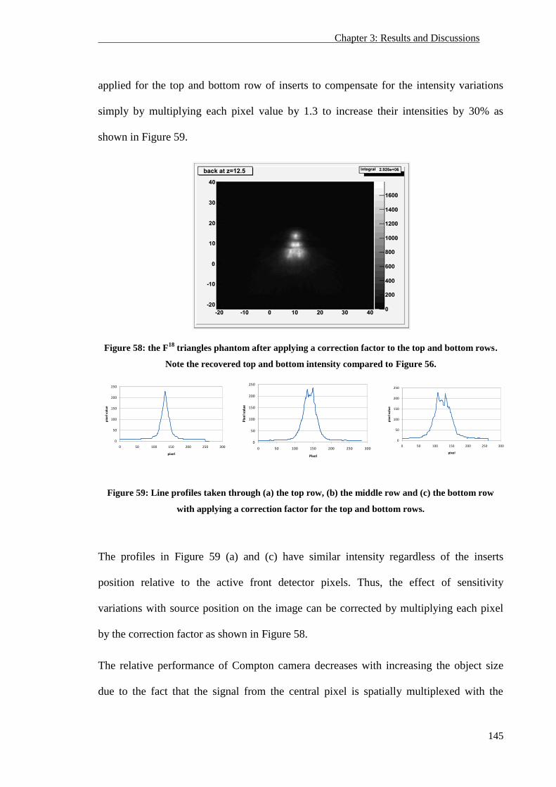
Chapter 3: Results and Discussions
145
applied for the top and bottom row of inserts to compensate for the intensity variations
simply by multiplying each pixel value by 1.3 to increase their intensities by 30% as
shown in Figure 59.
Figure 58: the F18
triangles phantom after applying a correction factor to the top and bottom rows.
Note the recovered top and bottom intensity compared to Figure 56.
Figure 59: Line profiles taken through (a) the top row, (b) the middle row and (c) the bottom row
with applying a correction factor for the top and bottom rows.
The profiles in Figure 59 (a) and (c) have similar intensity regardless of the inserts
position relative to the active front detector pixels. Thus, the effect of sensitivity
variations with source position on the image can be corrected by multiplying each pixel
by the correction factor as shown in Figure 58.
The relative performance of Compton camera decreases with increasing the object size
due to the fact that the signal from the central pixel is spatially multiplexed with the
0
50
100
150
200
250
0 50 100 150 200 250 300
pix
el v
alu
e
pixel
0
50
100
150
200
250
0 50 100 150 200 250 300
Pix
el v
alu
e
Pixel
0
50
100
150
200
250
0 50 100 150 200 250 300
pix
el v
alu
e
pixel
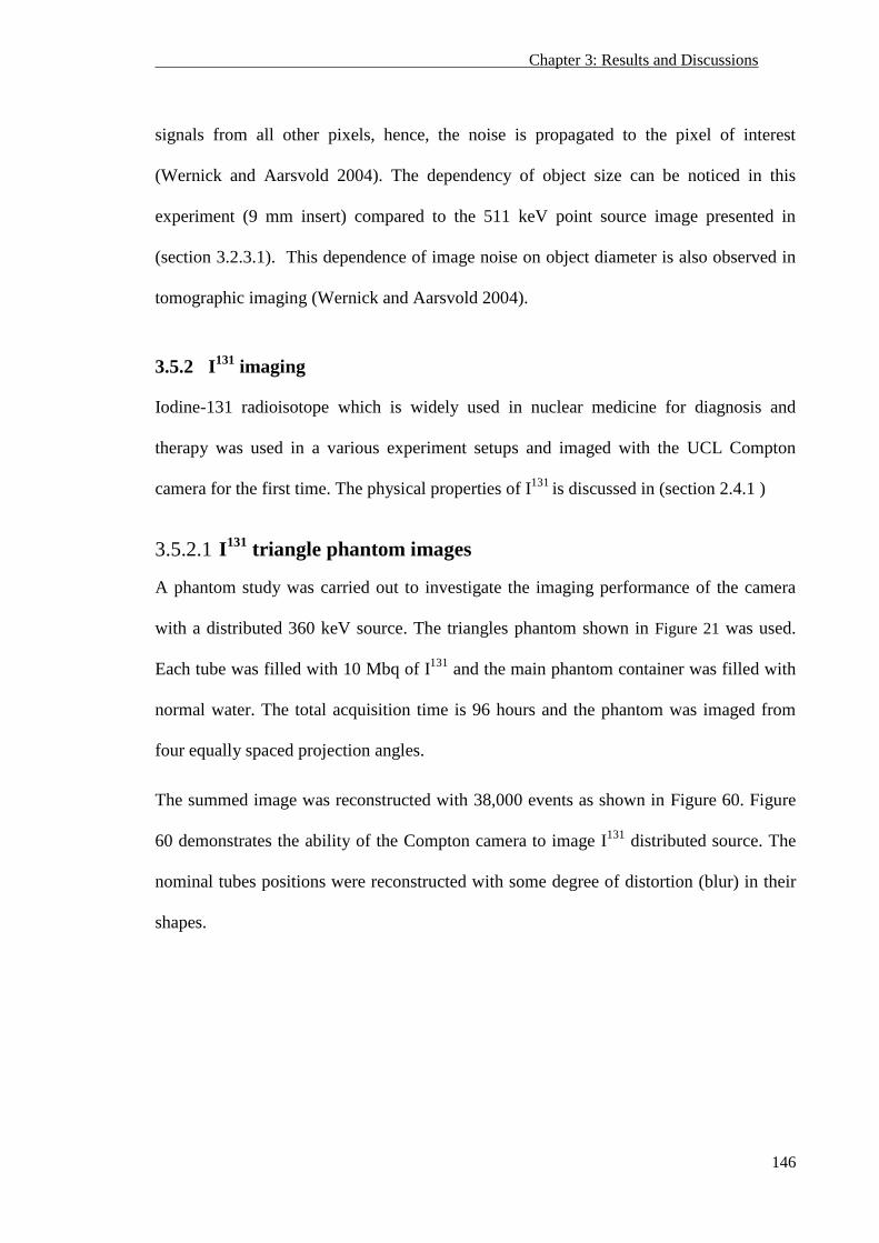
Chapter 3: Results and Discussions
146
signals from all other pixels, hence, the noise is propagated to the pixel of interest
(Wernick and Aarsvold 2004). The dependency of object size can be noticed in this
experiment (9 mm insert) compared to the 511 keV point source image presented in
(section 3.2.3.1). This dependence of image noise on object diameter is also observed in
tomographic imaging (Wernick and Aarsvold 2004).
3.5.2 I131
imaging
Iodine-131 radioisotope which is widely used in nuclear medicine for diagnosis and
therapy was used in a various experiment setups and imaged with the UCL Compton
camera for the first time. The physical properties of I131
is discussed in (section 2.4.1 )
3.5.2.1 I131 triangle phantom images
A phantom study was carried out to investigate the imaging performance of the camera
with a distributed 360 keV source. The triangles phantom shown in Figure 21 was used.
Each tube was filled with 10 Mbq of I131
and the main phantom container was filled with
normal water. The total acquisition time is 96 hours and the phantom was imaged from
four equally spaced projection angles.
The summed image was reconstructed with 38,000 events as shown in Figure 60. Figure
60 demonstrates the ability of the Compton camera to image I131
distributed source. The
nominal tubes positions were reconstructed with some degree of distortion (blur) in their
shapes.
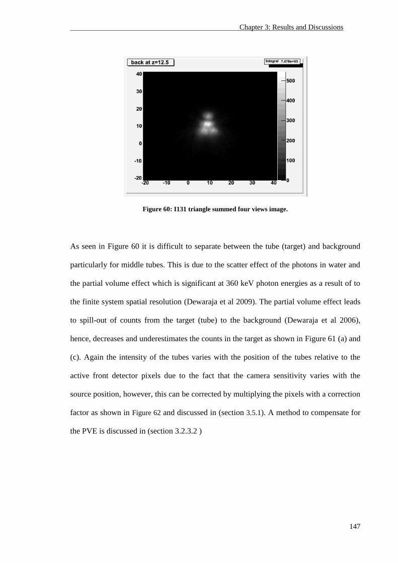
Chapter 3: Results and Discussions
147
Figure 60: I131 triangle summed four views image.
As seen in Figure 60 it is difficult to separate between the tube (target) and background
particularly for middle tubes. This is due to the scatter effect of the photons in water and
the partial volume effect which is significant at 360 keV photon energies as a result of to
the finite system spatial resolution (Dewaraja et al 2009). The partial volume effect leads
to spill-out of counts from the target (tube) to the background (Dewaraja et al 2006),
hence, decreases and underestimates the counts in the target as shown in Figure 61 (a) and
(c). Again the intensity of the tubes varies with the position of the tubes relative to the
active front detector pixels due to the fact that the camera sensitivity varies with the
source position, however, this can be corrected by multiplying the pixels with a correction
factor as shown in Figure 62 and discussed in (section 3.5.1). A method to compensate for
the PVE is discussed in (section 3.2.3.2 )
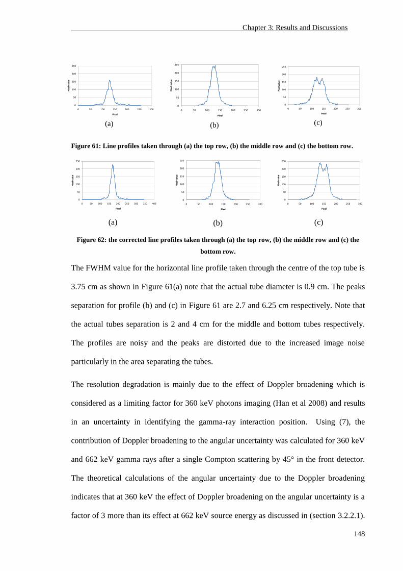
Chapter 3: Results and Discussions
148
(a) (b) (c)
Figure 61: Line profiles taken through (a) the top row, (b) the middle row and (c) the bottom row.
(a)
(b)
(c)
Figure 62: the corrected line profiles taken through (a) the top row, (b) the middle row and (c) the
bottom row.
The FWHM value for the horizontal line profile taken through the centre of the top tube is
3.75 cm as shown in Figure 61(a) note that the actual tube diameter is 0.9 cm. The peaks
separation for profile (b) and (c) in Figure 61 are 2.7 and 6.25 cm respectively. Note that
the actual tubes separation is 2 and 4 cm for the middle and bottom tubes respectively.
The profiles are noisy and the peaks are distorted due to the increased image noise
particularly in the area separating the tubes.
The resolution degradation is mainly due to the effect of Doppler broadening which is
considered as a limiting factor for 360 keV photons imaging (Han et al 2008) and results
in an uncertainty in identifying the gamma-ray interaction position. Using (7), the
contribution of Doppler broadening to the angular uncertainty was calculated for 360 keV
and 662 keV gamma rays after a single Compton scattering by 45° in the front detector.
The theoretical calculations of the angular uncertainty due to the Doppler broadening
indicates that at 360 keV the effect of Doppler broadening on the angular uncertainty is a
factor of 3 more than its effect at 662 keV source energy as discussed in (section 3.2.2.1).
0
50
100
150
200
250
0 50 100 150 200 250 300
Pix
el v
alu
e
Pixel
0
50
100
150
200
250
0 50 100 150 200 250 300
Pix
el v
alu
e
Pixel
0
50
100
150
200
250
0 50 100 150 200 250 300
Pix
el v
alu
e
Pixel
0
50
100
150
200
250
0 50 100 150 200 250 300 350 400
Pix
el v
alu
e
Pixel
0
50
100
150
200
250
0 50 100 150 200 250 300
Pix
el v
alu
e
Pixel
0
50
100
150
200
250
0 50 100 150 200 250 300
Pix
el v
alu
e
Pixel
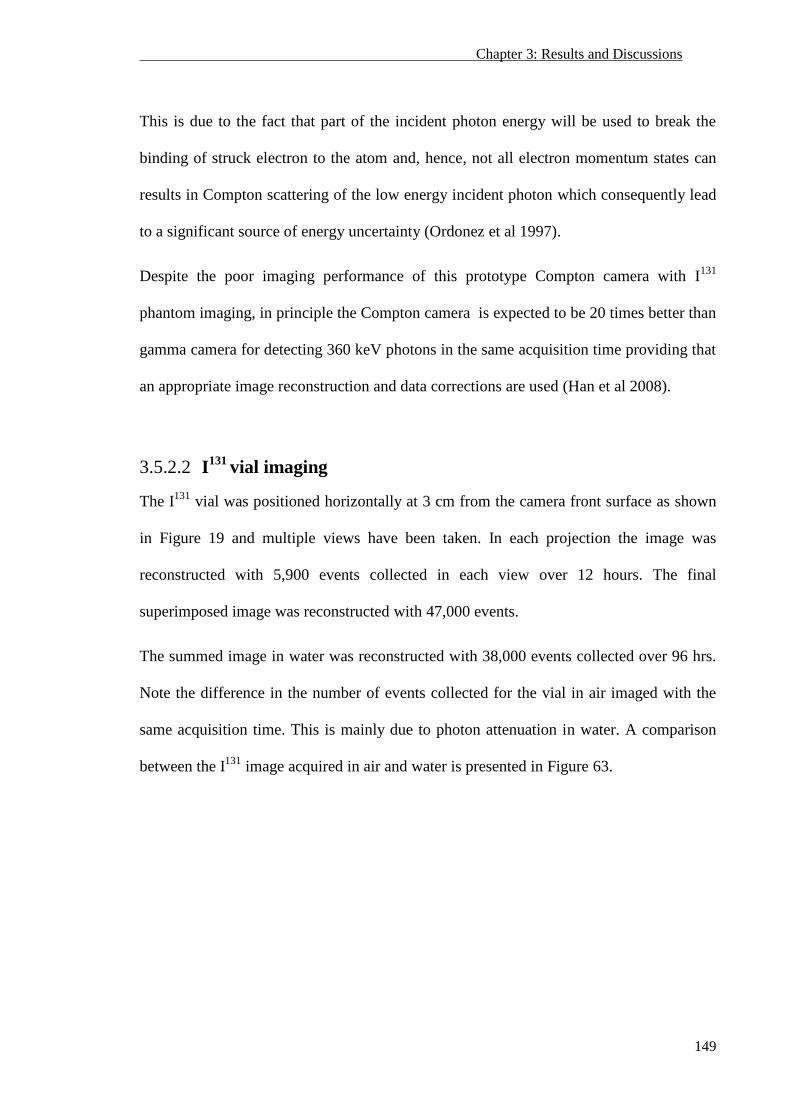
Chapter 3: Results and Discussions
149
This is due to the fact that part of the incident photon energy will be used to break the
binding of struck electron to the atom and, hence, not all electron momentum states can
results in Compton scattering of the low energy incident photon which consequently lead
to a significant source of energy uncertainty (Ordonez et al 1997).
Despite the poor imaging performance of this prototype Compton camera with I131
phantom imaging, in principle the Compton camera is expected to be 20 times better than
gamma camera for detecting 360 keV photons in the same acquisition time providing that
an appropriate image reconstruction and data corrections are used (Han et al 2008).
3.5.2.2 I131 vial imaging
The I131
vial was positioned horizontally at 3 cm from the camera front surface as shown
in Figure 19 and multiple views have been taken. In each projection the image was
reconstructed with 5,900 events collected in each view over 12 hours. The final
superimposed image was reconstructed with 47,000 events.
The summed image in water was reconstructed with 38,000 events collected over 96 hrs.
Note the difference in the number of events collected for the vial in air imaged with the
same acquisition time. This is mainly due to photon attenuation in water. A comparison
between the I131
image acquired in air and water is presented in Figure 63.
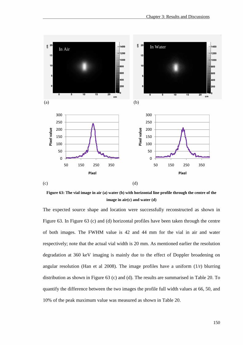
Chapter 3: Results and Discussions
150
(a) (b)
(c) (d)
Figure 63: The vial image in air (a) water (b) with horizontal line profile through the centre of the
image in air(c) and water (d)
The expected source shape and location were successfully reconstructed as shown in
Figure 63. In Figure 63 (c) and (d) horizontal profiles have been taken through the centre
of both images. The FWHM value is 42 and 44 mm for the vial in air and water
respectively; note that the actual vial width is 20 mm. As mentioned earlier the resolution
degradation at 360 keV imaging is mainly due to the effect of Doppler broadening on
angular resolution (Han et al 2008). The image profiles have a uniform (1/r) blurring
distribution as shown in Figure 63 (c) and (d). The results are summarised in Table 20. To
quantify the difference between the two images the profile full width values at 66, 50, and
10% of the peak maximum value was measured as shown in Table 20.
0
50
100
150
200
250
300
50 150 250 350
Pix
el v
alu
e
Pixel
0
50
100
150
200
250
300
50 150 250 350
Pix
el v
alu
e
Pixel
In Air In Water
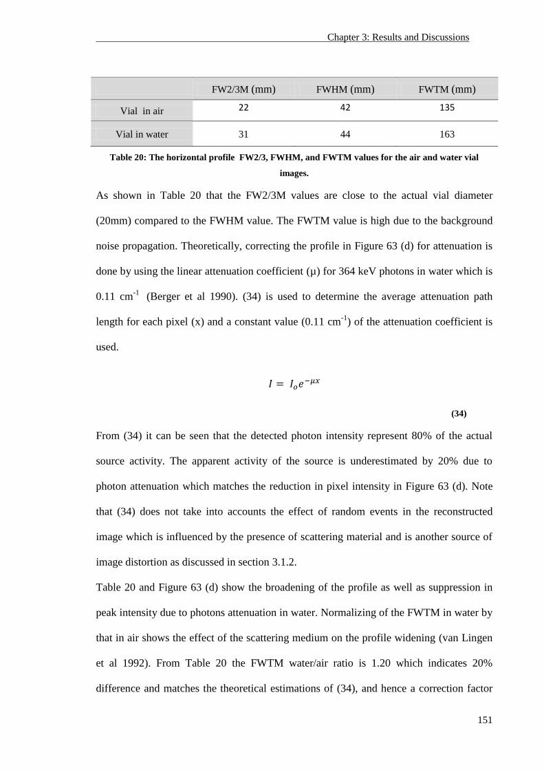
Chapter 3: Results and Discussions
151
FW2/3M (mm) FWHM (mm) FWTM (mm)
Vial in air 22 42 135
Vial in water 31 44 163
Table 20: The horizontal profile FW2/3, FWHM, and FWTM values for the air and water vial
images.
As shown in Table 20 that the FW2/3M values are close to the actual vial diameter
(20mm) compared to the FWHM value. The FWTM value is high due to the background
noise propagation. Theoretically, correcting the profile in Figure 63 (d) for attenuation is
done by using the linear attenuation coefficient (µ) for 364 keV photons in water which is
0.11 cm-1
(Berger et al 1990). (34) is used to determine the average attenuation path
length for each pixel (x) and a constant value (0.11 cm-1
) of the attenuation coefficient is
used.
(34)
From (34) it can be seen that the detected photon intensity represent 80% of the actual
source activity. The apparent activity of the source is underestimated by 20% due to
photon attenuation which matches the reduction in pixel intensity in Figure 63 (d). Note
that (34) does not take into accounts the effect of random events in the reconstructed
image which is influenced by the presence of scattering material and is another source of
image distortion as discussed in section 3.1.2.
Table 20 and Figure 63 (d) show the broadening of the profile as well as suppression in
peak intensity due to photons attenuation in water. Normalizing of the FWTM in water by
that in air shows the effect of the scattering medium on the profile widening (van Lingen
et al 1992). From Table 20 the FWTM water/air ratio is 1.20 which indicates 20%
difference and matches the theoretical estimations of (34), and hence a correction factor
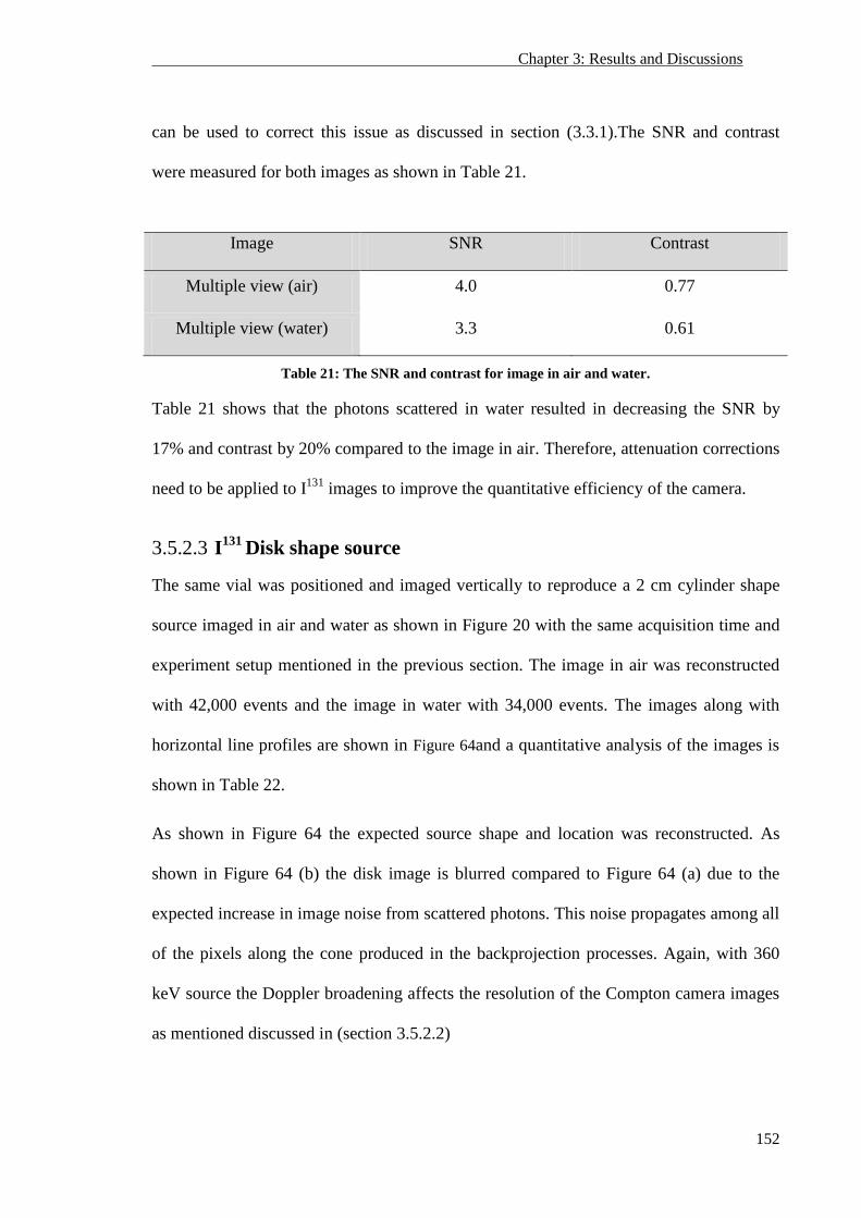
Chapter 3: Results and Discussions
152
can be used to correct this issue as discussed in section ( 3.3.1).The SNR and contrast
were measured for both images as shown in Table 21.
Image SNR Contrast
Multiple view (air) 4.0 0.77
Multiple view (water) 3.3 0.61
Table 21: The SNR and contrast for image in air and water.
Table 21 shows that the photons scattered in water resulted in decreasing the SNR by
17% and contrast by 20% compared to the image in air. Therefore, attenuation corrections
need to be applied to I131
images to improve the quantitative efficiency of the camera.
3.5.2.3 I131 Disk shape source
The same vial was positioned and imaged vertically to reproduce a 2 cm cylinder shape
source imaged in air and water as shown in Figure 20 with the same acquisition time and
experiment setup mentioned in the previous section. The image in air was reconstructed
with 42,000 events and the image in water with 34,000 events. The images along with
horizontal line profiles are shown in Figure 64and a quantitative analysis of the images is
shown in Table 22.
As shown in Figure 64 the expected source shape and location was reconstructed. As
shown in Figure 64 (b) the disk image is blurred compared to Figure 64 (a) due to the
expected increase in image noise from scattered photons. This noise propagates among all
of the pixels along the cone produced in the backprojection processes. Again, with 360
keV source the Doppler broadening affects the resolution of the Compton camera images
as mentioned discussed in (section 3.5.2.2)
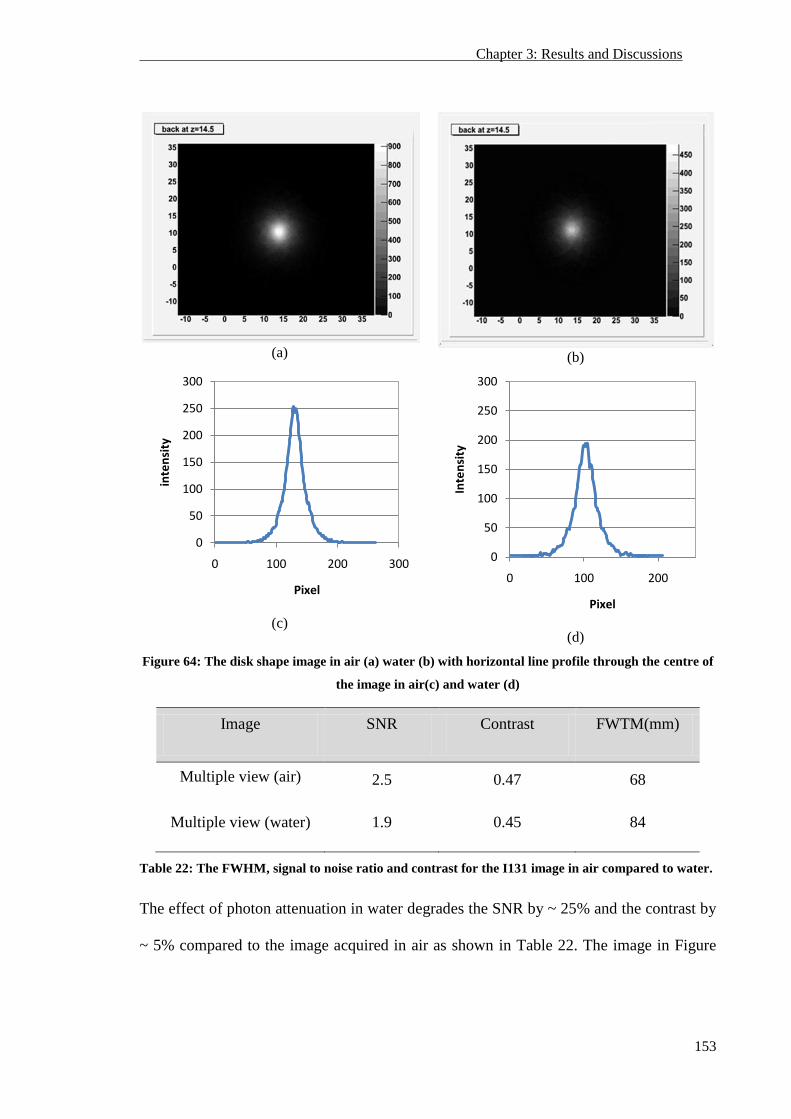
Chapter 3: Results and Discussions
153
(a)
(b)
(c)
(d)
Figure 64: The disk shape image in air (a) water (b) with horizontal line profile through the centre of
the image in air(c) and water (d)
Image SNR Contrast FWTM(mm)
Multiple view (air) 2.5 0.47 68
Multiple view (water) 1.9 0.45 84
Table 22: The FWHM, signal to noise ratio and contrast for the I131 image in air compared to water.
The effect of photon attenuation in water degrades the SNR by ~ 25% and the contrast by
~ 5% compared to the image acquired in air as shown in Table 22. The image in Figure
0
50
100
150
200
250
300
0 100 200 300
inte
nsi
ty
Pixel
0
50
100
150
200
250
300
0 100 200
Inte
nsi
ty
Pixel
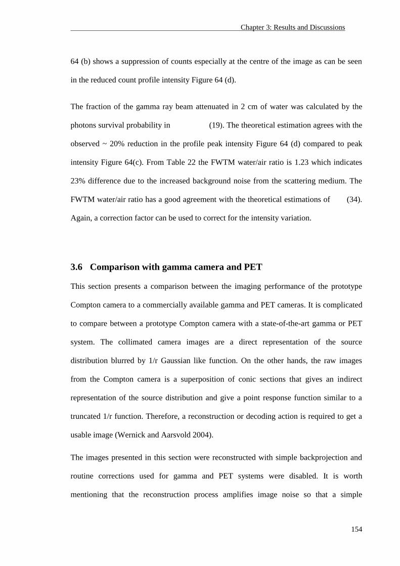
Chapter 3: Results and Discussions
154
64 (b) shows a suppression of counts especially at the centre of the image as can be seen
in the reduced count profile intensity Figure 64 (d).
The fraction of the gamma ray beam attenuated in 2 cm of water was calculated by the
photons survival probability in (19). The theoretical estimation agrees with the
observed ~ 20% reduction in the profile peak intensity Figure 64 (d) compared to peak
intensity Figure 64(c). From Table 22 the FWTM water/air ratio is 1.23 which indicates
23% difference due to the increased background noise from the scattering medium. The
FWTM water/air ratio has a good agreement with the theoretical estimations of (34).
Again, a correction factor can be used to correct for the intensity variation.
3.6 Comparison with gamma camera and PET
This section presents a comparison between the imaging performance of the prototype
Compton camera to a commercially available gamma and PET cameras. It is complicated
to compare between a prototype Compton camera with a state-of-the-art gamma or PET
system. The collimated camera images are a direct representation of the source
distribution blurred by 1/r Gaussian like function. On the other hands, the raw images
from the Compton camera is a superposition of conic sections that gives an indirect
representation of the source distribution and give a point response function similar to a
truncated 1/r function. Therefore, a reconstruction or decoding action is required to get a
usable image (Wernick and Aarsvold 2004).
The images presented in this section were reconstructed with simple backprojection and
routine corrections used for gamma and PET systems were disabled. It is worth
mentioning that the reconstruction process amplifies image noise so that a simple
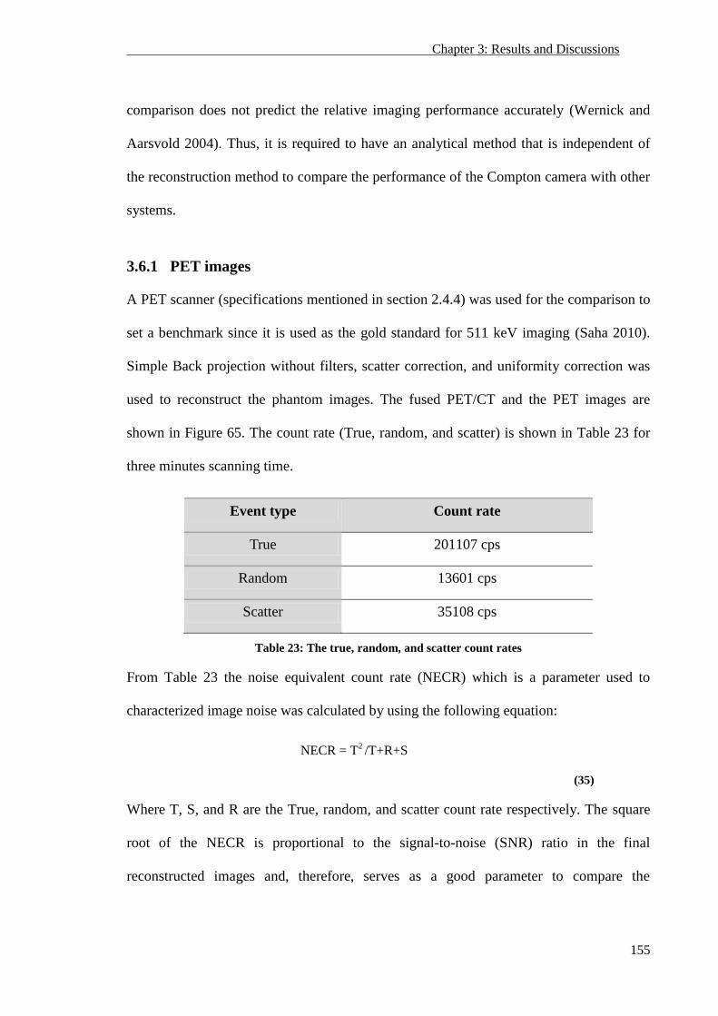
Chapter 3: Results and Discussions
155
comparison does not predict the relative imaging performance accurately (Wernick and
Aarsvold 2004). Thus, it is required to have an analytical method that is independent of
the reconstruction method to compare the performance of the Compton camera with other
systems.
3.6.1 PET images
A PET scanner (specifications mentioned in section 2.4.4) was used for the comparison to
set a benchmark since it is used as the gold standard for 511 keV imaging (Saha 2010).
Simple Back projection without filters, scatter correction, and uniformity correction was
used to reconstruct the phantom images. The fused PET/CT and the PET images are
shown in Figure 65. The count rate (True, random, and scatter) is shown in Table 23 for
three minutes scanning time.
Event type Count rate
True 201107 cps
Random 13601 cps
Scatter 35108 cps
Table 23: The true, random, and scatter count rates
From Table 23 the noise equivalent count rate (NECR) which is a parameter used to
characterized image noise was calculated by using the following equation:
NECR = T2 /T+R+S
(35)
Where T, S, and R are the True, random, and scatter count rate respectively. The square
root of the NECR is proportional to the signal-to-noise (SNR) ratio in the final
reconstructed images and, therefore, serves as a good parameter to compare the
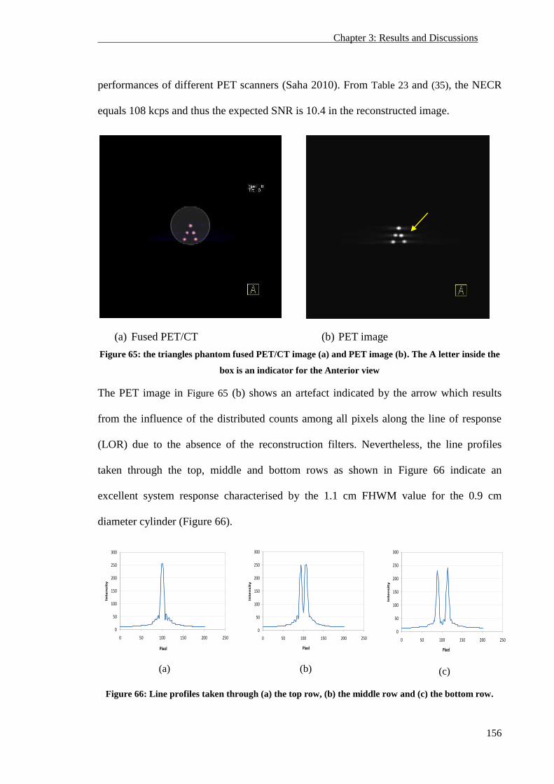
Chapter 3: Results and Discussions
156
performances of different PET scanners (Saha 2010). From Table 23 and (35), the NECR
equals 108 kcps and thus the expected SNR is 10.4 in the reconstructed image.
(a) Fused PET/CT (b) PET image
Figure 65: the triangles phantom fused PET/CT image (a) and PET image (b). The A letter inside the
box is an indicator for the Anterior view
The PET image in Figure 65 (b) shows an artefact indicated by the arrow which results
from the influence of the distributed counts among all pixels along the line of response
(LOR) due to the absence of the reconstruction filters. Nevertheless, the line profiles
taken through the top, middle and bottom rows as shown in Figure 66 indicate an
excellent system response characterised by the 1.1 cm FHWM value for the 0.9 cm
diameter cylinder (Figure 66).
(a)
(b)
(c)
Figure 66: Line profiles taken through (a) the top row, (b) the middle row and (c) the bottom row.
0
50
100
150
200
250
300
0 50 100 150 200 250
Inte
nsit
y
Pixel
0
50
100
150
200
250
300
0 50 100 150 200 250
Inte
nsit
y
Pixel
0
50
100
150
200
250
300
0 50 100 150 200 250
Inte
nsit
y
Pixel
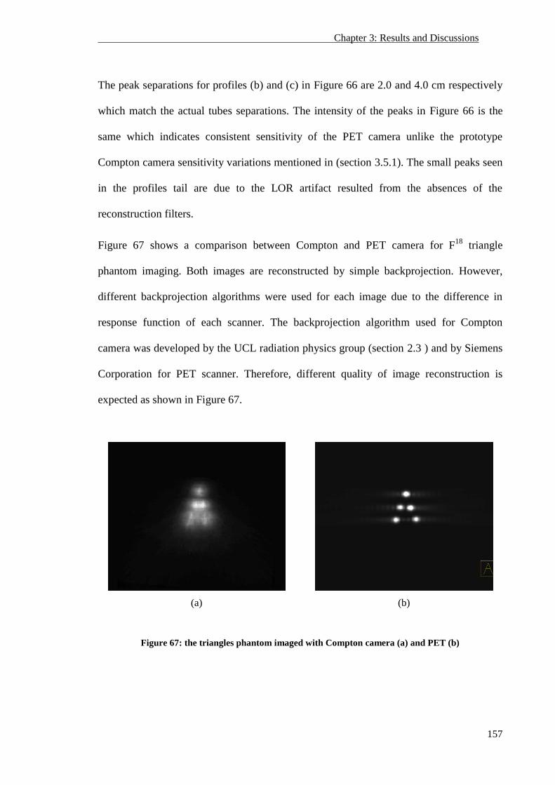
Chapter 3: Results and Discussions
157
The peak separations for profiles (b) and (c) in Figure 66 are 2.0 and 4.0 cm respectively
which match the actual tubes separations. The intensity of the peaks in Figure 66 is the
same which indicates consistent sensitivity of the PET camera unlike the prototype
Compton camera sensitivity variations mentioned in (section 3.5.1). The small peaks seen
in the profiles tail are due to the LOR artifact resulted from the absences of the
reconstruction filters.
Figure 67 shows a comparison between Compton and PET camera for F18
triangle
phantom imaging. Both images are reconstructed by simple backprojection. However,
different backprojection algorithms were used for each image due to the difference in
response function of each scanner. The backprojection algorithm used for Compton
camera was developed by the UCL radiation physics group (section 2.3 ) and by Siemens
Corporation for PET scanner. Therefore, different quality of image reconstruction is
expected as shown in Figure 67.
(a)
(b)
Figure 67: the triangles phantom imaged with Compton camera (a) and PET (b)
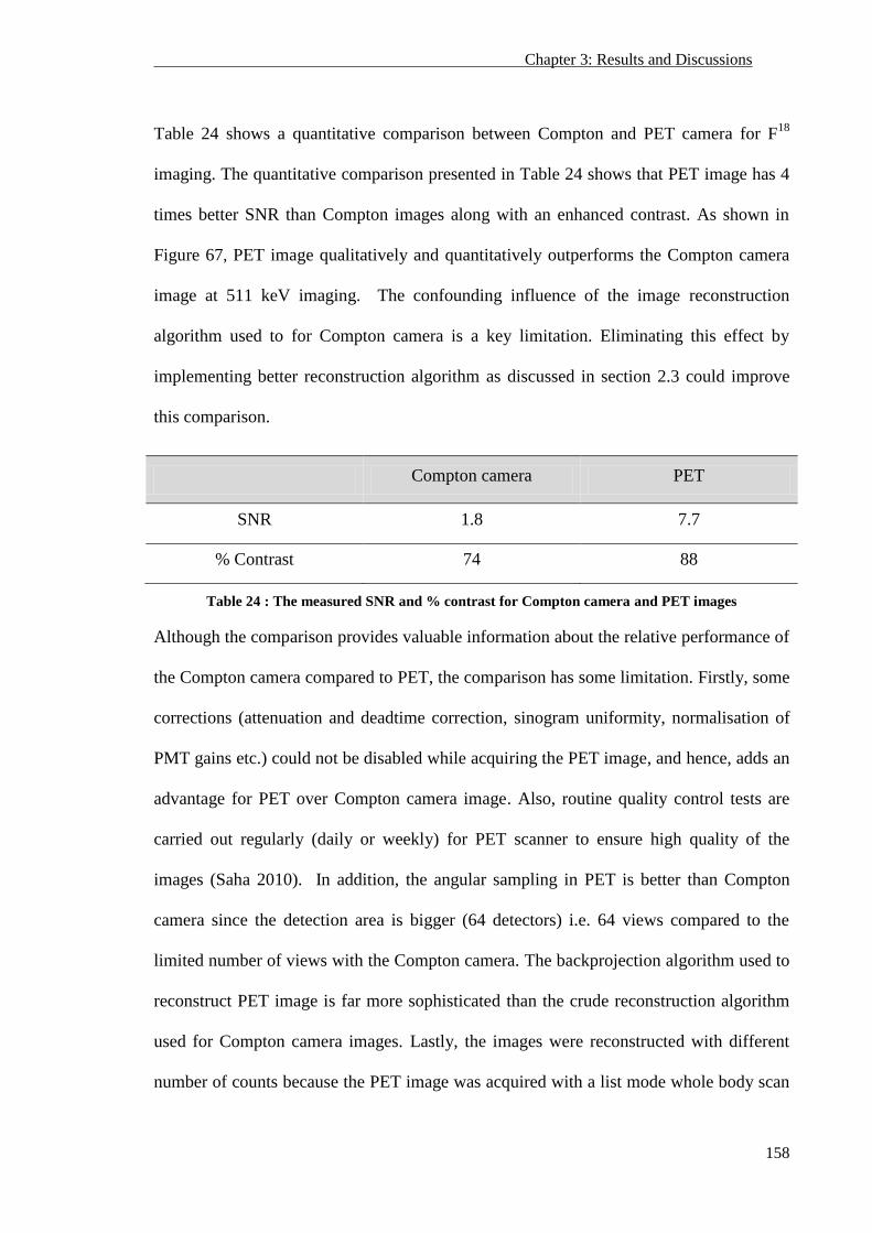
Chapter 3: Results and Discussions
158
Table 24 shows a quantitative comparison between Compton and PET camera for F18
imaging. The quantitative comparison presented in Table 24 shows that PET image has 4
times better SNR than Compton images along with an enhanced contrast. As shown in
Figure 67, PET image qualitatively and quantitatively outperforms the Compton camera
image at 511 keV imaging. The confounding influence of the image reconstruction
algorithm used to for Compton camera is a key limitation. Eliminating this effect by
implementing better reconstruction algorithm as discussed in section 2.3 could improve
this comparison.
Compton camera PET
SNR 1.8 7.7
% Contrast 74 88
Table 24 : The measured SNR and % contrast for Compton camera and PET images
Although the comparison provides valuable information about the relative performance of
the Compton camera compared to PET, the comparison has some limitation. Firstly, some
corrections (attenuation and deadtime correction, sinogram uniformity, normalisation of
PMT gains etc.) could not be disabled while acquiring the PET image, and hence, adds an
advantage for PET over Compton camera image. Also, routine quality control tests are
carried out regularly (daily or weekly) for PET scanner to ensure high quality of the
images (Saha 2010). In addition, the angular sampling in PET is better than Compton
camera since the detection area is bigger (64 detectors) i.e. 64 views compared to the
limited number of views with the Compton camera. The backprojection algorithm used to
reconstruct PET image is far more sophisticated than the crude reconstruction algorithm
used for Compton camera images. Lastly, the images were reconstructed with different
number of counts because the PET image was acquired with a list mode whole body scan
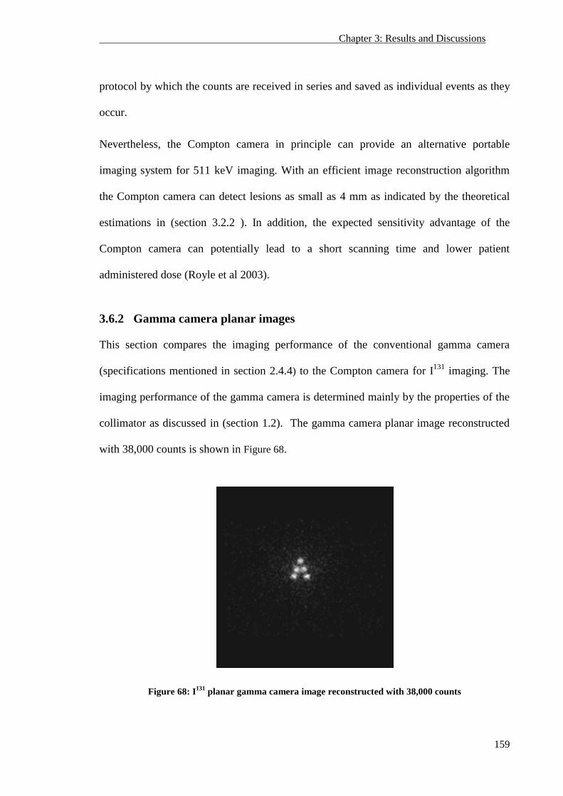
Chapter 3: Results and Discussions
159
protocol by which the counts are received in series and saved as individual events as they
occur.
Nevertheless, the Compton camera in principle can provide an alternative portable
imaging system for 511 keV imaging. With an efficient image reconstruction algorithm
the Compton camera can detect lesions as small as 4 mm as indicated by the theoretical
estimations in (section 3.2.2 ). In addition, the expected sensitivity advantage of the
Compton camera can potentially lead to a short scanning time and lower patient
administered dose (Royle et al 2003).
3.6.2 Gamma camera planar images
This section compares the imaging performance of the conventional gamma camera
(specifications mentioned in section 2.4.4) to the Compton camera for I131
imaging. The
imaging performance of the gamma camera is determined mainly by the properties of the
collimator as discussed in (section 1.2). The gamma camera planar image reconstructed
with 38,000 counts is shown in Figure 68.
Figure 68: I131
planar gamma camera image reconstructed with 38,000 counts
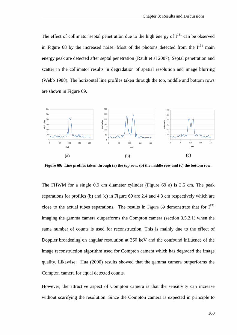
Chapter 3: Results and Discussions
160
The effect of collimator septal penetration due to the high energy of I131
can be observed
in Figure 68 by the increased noise. Most of the photons detected from the I131
main
energy peak are detected after septal penetration (Rault et al 2007). Septal penetration and
scatter in the collimator results in degradation of spatial resolution and image blurring
(Webb 1988). The horizontal line profiles taken through the top, middle and bottom rows
are shown in Figure 69.
(a)
(b)
(c)
Figure 69: Line profiles taken through (a) the top row, (b) the middle row and (c) the bottom row.
The FHWM for a single 0.9 cm diameter cylinder (Figure 69 a) is 3.5 cm. The peak
separations for profiles (b) and (c) in Figure 69 are 2.4 and 4.3 cm respectively which are
close to the actual tubes separations. The results in Figure 69 demonstrate that for I131
imaging the gamma camera outperforms the Compton camera (section 3.5.2.1) when the
same number of counts is used for reconstruction. This is mainly due to the effect of
Doppler broadening on angular resolution at 360 keV and the confound influence of the
image reconstruction algorithm used for Compton camera which has degraded the image
quality. Likewise, Hua (2000) results showed that the gamma camera outperforms the
Compton camera for equal detected counts.
However, the attractive aspect of Compton camera is that the sensitivity can increase
without scarifying the resolution. Since the Compton camera is expected in principle to
0
50
100
150
200
250
300
0 50 100 150 200
pix
el v
alu
e
Pixel
0
50
100
150
200
250
300
0 50 100 150 200
pix
el v
alu
e
pixel
0
50
100
150
200
250
300
0 50 100 150 200
pix
el v
alu
e
pixel
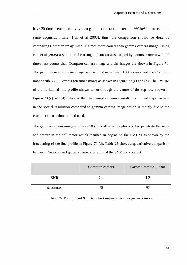
Chapter 3: Results and Discussions
161
have 20 times better sensitivity than gamma camera for detecting 360 keV photons in the
same acquisition time (Han et al 2008), thus, the comparison should be done by
comparing Compton image with 20 times more counts than gamma camera image. Using
Han et al (2008) assumption the triangle phantom was imaged by gamma camera with 20
times less counts than Compton camera image and the images are shown in Figure 70.
The gamma camera planar image was reconstructed with 1900 counts and the Compton
image with 38,000 events (20 times more) as shown in Figure 70 (a) and (b). The FWHM
of the horizontal line profile shown taken through the centre of the top row shown in
Figure 70 (c) and (d) indicates that the Compton camera result in a limited improvement
in the spatial resolution compared to gamma camera image which is mainly due to the
crude reconstruction method used.
The gamma camera image in Figure 70 (b) is affected by photons that penetrate the septa
and scatter in the collimator which resulted in degrading the FWHM as shown by the
broadening of the line profile in Figure 70 (d). Table 25 shows a quantitative comparison
between Compton and gamma camera in terms of the SNR and contrast.
Compton camera Gamma camera-Planar
SNR 2.4 1.2
% contrast 78 97
Table 25: The SNR and % contrast for Compton camera vs. gamma camera
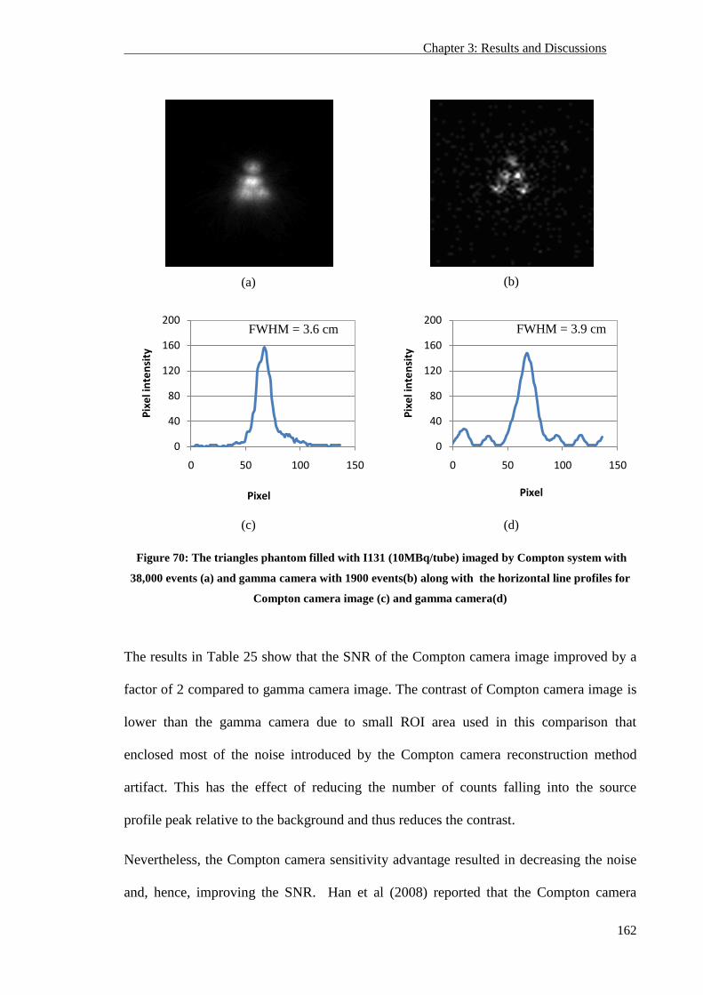
Chapter 3: Results and Discussions
162
(a)
(b)
(c)
(d)
Figure 70: The triangles phantom filled with I131 (10MBq/tube) imaged by Compton system with
38,000 events (a) and gamma camera with 1900 events(b) along with the horizontal line profiles for
Compton camera image (c) and gamma camera(d)
The results in Table 25 show that the SNR of the Compton camera image improved by a
factor of 2 compared to gamma camera image. The contrast of Compton camera image is
lower than the gamma camera due to small ROI area used in this comparison that
enclosed most of the noise introduced by the Compton camera reconstruction method
artifact. This has the effect of reducing the number of counts falling into the source
profile peak relative to the background and thus reduces the contrast.
Nevertheless, the Compton camera sensitivity advantage resulted in decreasing the noise
and, hence, improving the SNR. Han et al (2008) reported that the Compton camera
0
40
80
120
160
200
0 50 100 150
Pix
el i
nte
nsi
ty
Pixel
0
40
80
120
160
200
0 50 100 150
Pix
el i
nte
nsi
ty
Pixel
FWHM = 3.9 cm FWHM = 3.6 cm
Chapter 3: Results and Discussions
163
showed better noise performance than gamma camera when imaging source size below
~10 mm diameter size. Therefore, the results show that the Compton camera is a
promising imaging system for I131
imaging that can provide an improved sensitivity and
better noise performance than gamma camera, and hence, provides better diagnostic
quality and increase patient comfort by decreasing the scanning time. This comparison
can be improved by employing a more sophisticated image reconstruction algorithm e.g.
MLEM as indicated by Han et al (2008) in order to improve the achievable image quality.
Chapter 4: Conclusion and Future Work
164
4 Conclusions and Future Work
This chapter summarizes the work and results presented in previous chapters.
Conclusions are made based on experimental results and theoretical analysis. Future work
for improving the Compton camera system design, imaging performance, image
reconstruction algorithm and readout electronics are described.
4.1 Summary
The main goal of this research is to improve nuclear medicine imagining by using
electronic photon collimation technique. In this study, an electronic collimation method
based on Compton scattering imaging has been introduced and evaluated. The results
presented in this work show how Compton scattered events in the Compton camera
system may be successfully used for imaging. This thesis demonstrates the current
performance of the UCL Compton camera system and provides a point from which
additional development work may carry on. This is likely to focus on three main areas of
the system; implementation of high-count-rate capabilities readout digital electronics,
development of online data processing and PSA techniques and the innovation of
sophisticated image reconstruction algorithms.
In Chapter 1, the general principles of gamma ray imaging in nuclear medicine, gamma
camera, and PET were described. The physical limitations of current systems have been
identified and compared to current approaches of improving camera performance. Then
the principle, advantages, and the historical development of an electronic collimation
technique based on Compton scattering physics have been demonstrated.
Chapter 4: Conclusion and Future Work
165
Chapter 2 demonstrate the materials and methods used in this work. The UCL HPGe
prototype Compton camera design, specifications, and associated readout electronics were
explained in details. The coincidence imaging operation mode, image reconstruction, and
experimental setup have been demonstrated. In addition, the data analysis tools used to
quantify the image quality was explained.
The results obtained for this work are shown in chapter 3. The results include the
interaction probabilities, system performance characteristics and the imaging performance
of the Compton camera with different source distributions. The results were interpreted
quantitatively and compared to other cameras used in nuclear medicine.
Conclusions for the work presented in this work were drawn and future directions were
defined in chapter 4.
4.2 Conclusions
The Compton camera offers many potential advantages for gamma-ray imaging
applications. In principle, the Compton camera can provide better spatial resolution and
sensitivity for high gamma-ray energies (>300 keV) compared to gamma camera.
Therefore, a variety of high energy possible applications can benefit from Compton
imaging: including I131
(364 keV) for thyroid and monoclonal antibodies, In113m
(393
keV) which can be used as a substitute for In111
to label blood cells in order to investigate
infections and inflammation sites, and positron emitting isotopes.
Although there are a number of limitations in the current prototype camera some
potentially useful qualities have been demonstrated and distributed sources have been
imaged. This thesis shows that the multiple-view technique results in a significant
improvement in the image quality by minimizing the image geometrical distortion and is
Chapter 4: Conclusion and Future Work
166
an effective way to accurately reconstruct the source distribution, and hence, provides a
practical way to the Compton camera development research field to improve the quality
of the images obtained. To the best of my knowledge, this work present experimentally
for the first time the ability of a Ge Compton camera for quantitative I131
and F18
phantom
imaging . In addition, a quantitative comparison between Compton camera and gamma
camera for I131
imaging and with PET scanner for F18
imaging was carried out. This work
confirmed that the Compton camera can be used with a factor of 2 improvements in the
SNR compared to the mechanically collimated gamma camera for I131
. Even though PET
scanner outperforms the Compton camera in 511 keV imaging, the Compton camera in
principle can provide an alternative portable imaging system with high spatial resolution
and sensitivity for 511 keV imaging. A portable system provides the possibility of
obtaining intra-operative images that can help to confirm the location of lesion and
whether it is correctly removed. Thus, avoiding future surgical procedures. More focus is
needed by the Compton camera researchers to the potentials of the camera with these two
widely used nuclear medicine radioisotopes.
The key limitations in the current prototype are acquisition time, processing time and
image reconstruction. The current arrangement for the readout electronics employed in
this camera have shown significant limitations at high count rates, which has lead to long
acquisition times in the current prototype. However, techniques are available to
significantly improve this and an improved parallel approach is currently being
implemented. The offline post-processing method to select coincidence events currently
being used also is time consuming. The system collects the deposited charge in all pixels
regardless of where the interaction actually occurred and then converts it to digital
numbers before passing them to a PC sequentially. Thus, this method results in a high
Chapter 4: Conclusion and Future Work
167
dead time, pulse pileup, and a data bottle neck. A fast online coincidence events selection
algorithm is also being developed.
Theoretical investigation of the probabilities of interaction with the scatter and absorber
detectors was carried out. The results showed that the energy deposited in the both
detectors is a function of source energy and with using high source energy (>360 keV)
more than 90% of the photons will interact with the detectors by Compton scattering.
Based on the calculated front energies in Table 9 the energy threshold was set to 10 keV
for all measurement (unless mentioned) to accept only gamma-ray photons scattered by >
20° in the front detector and minimize the detector noise effect. The uncertainty in
measuring the scatter angle increases by using low gamma-ray source energy due to the
very little energy measured in the front detector as well as the effect of Doppler
broadening.
The camera performance characteristics were investigated. The energy resolution for the
camera achieved using the MWD energy extraction algorithm is 1.2 % and 0.7% for 356
and 662 keV respectively. The results showed that energy resolution values depend
strongly on the width of the deconvolution window and a minimum window of 8 µs is
needed to obtain good energy resolution, and the best FWHM was obtained with 11 µs
window.
The angular resolution was estimated theoretically using Singh’s (1983) formulas and
measured experimentally by imaging different point source energies. The theoretical
estimation showed that the angular uncertainty is dominated by the geometrical
contribution of the detectors. Different radioisotope point sources (Ba133
, Na22
, and Cs137
)
were imaged and reconstructed for the first time with the UCL camera. The measured
FWHM at 5 cm are 7.5, 7.2, and 6.9 ± 2 mm for 356, 511 and 662 keV gamma energies
Chapter 4: Conclusion and Future Work
168
respectively which translate to angular resolutions 8.5°, 8.2°, and 7.8° for 356, 511 and
662 keV gamma energies respectively.
The disagreement between theoretical and experimental values is due to the fact that the
effect of the random events, dead time, and the reconstruction algorithm decoding penalty
were not considered in the theoretical calculation. In addition, The results show that the
spatial resolution is distance dependent.
Due to the limited active area and readout electronics a technique to reconstruct the point
source image with a uniform symmetric distribution by acquiring multiple views was
carried out. The results show that this technique improved the image spatial resolution.
This technique was used to maximize the information yield from Compton camera images
and simulate the proposed full camera. This technique proved that the camera FWHM and
SNR can be improved by populating the full camera pixels.
The camera imaging performance with extended source distributions (line source, ring
source, and Perspex phantom) were investigated and imaged and successfully
reconstructed. In addition, the results showed the ability of this system to resolve two
point sources separated by 0.3 mm. Thus, this system has the potential to detect small
lesions separated by few millimeters.
The measured intrinsic efficiency of the camera with the current limited pixel geometry is
3.5x10⁻¹⁰
.The detection efficiency for the experimental measured efficiency is lower than
theoretically estimated efficiency (in section 2.9.2) by five orders of magnitude due to the
limited number of pixels (31 pixels) and the counting limitations of the system.
The system timing resolution was measured by taking the FWHM value for the
coincidence-timing spectrum shown in Figure 42. The measured system electronic time
resolution is about 70 ns. Therefore, the coincidence time window was set to 75 ns which
Chapter 4: Conclusion and Future Work
169
are sufficient to pass most of the true coincidence events. The SNR improves linearly
with decreasing the time window width due to the improved true/random events ratio
while scarifying the number of coincidence counts decrease.
The count rate performance of the system is limited by the relatively slow readout
electronics as revealed by the poor timing resolution. Under high incident photons flux or
with increasing the number of active pixels bottle neck behaviour in the data output pipe
was observed. From Figure 46 it can be noticed that the maximum data rate is ~ 1.85
Mbytes/sec which translates to 31 counts per second. The estimated system dead time is
32 milliseconds. The results show that the counting performance has strong dependence
on the number of back pixels compared to the front pixels due to the fact that the back
pixels are used to initiate triggering and readout sequences.
The faction of scatter photons detected depends mainly on the density of the scattering
medium, source energy, the depth of the source, detector energy resolution and the energy
window width. The scatter fraction increases with increasing the energy window width.
Using narrow energy window width is possible with the excellent germanium energy
resolution but at the expense of sensitivity.
The images in section 3.5 present the first images of Fluorine-18 and Iodine-131 obtained
with the UCL prototype Compton camera. The expected phantom shape and insert
locations were successfully reconstructed. The intensity of the inserts varies according to
their position relative to the active front detector pixels due to the fact that the camera
sensitivity varies with the source position. However, a correction factor was applied for
the top and bottom row of inserts to compensate for the intensity variations. The
resolution degradation for Iodine-131 imaging is mainly due to the effect of Doppler
Chapter 4: Conclusion and Future Work
170
broadening. The theoretical calculations of the angular uncertainty due to the Doppler
broadening indicates that at 360 keV the effect of Doppler broadening on the angular
uncertainty is a factor of 3 more than its effect at 662 keV source energy. These results
showed the feasibility of using Compton camera for nuclear medicine studies providing
that the current prototype limitations are treated.
A comparison between the imaging performances of the prototype Compton camera to a
commercially available PET camera is presented in (section 3.5.1). The images were
reconstructed by simple backprojection algorithm. However, different algorithms were
used for each image due to the difference in response function of each scanner. The
results show that PET qualitatively outperforms the Compton camera at 511 keV imaging
and achieves 4 times better SNR. Although the comparison provides valuable information
about the relative performance of the Compton camera compared to PET, the comparison
has some limitation. Firstly, some corrections could not be disabled while acquiring the
PET image, and hence, adds an advantage for PET over Compton camera image. In
addition, the angular sampling in PET is superior since the detection area is bigger (64
detectors) i.e. 64 views compared to the limited number of views with the Compton
camera. Finally, the backprojection algorithm used to reconstruct PET image is more
sophisticated than the crude reconstruction algorithm used for Compton camera images.
Therefore, this comparison can be improve by using a statistical image reconstruction
method (e.g. MLEM) or analytically simulate both systems and use the same number of
counts for image reconstruction with disabling all filters and corrections in PET to have
like with like comparison.
Section 3.5.2 compares the imaging performance of the conventional gamma camera to
the Compton camera for I131
imaging. The results show that the gamma camera
outperforms the Compton camera for I131
imaging when the same number of counts is
Chapter 4: Conclusion and Future Work
171
used for reconstruction. This is mainly due to the effect of Doppler broadening on angular
resolution at 360 keV and the confound influence of the image reconstruction algorithm
used for Compton camera. However, the attractive aspect of Compton camera is that the
sensitivity can increase without scarifying the resolution. The Compton camera is
expected in principle to have 20 times better sensitivity than gamma camera for detecting
360 keV photons in the same acquisition time (Han et al 2008). Therefore, another
comparison was done by comparing Compton image with 20 times more counts than
gamma camera image. The results show that the SNR of the Compton camera image
improved by a factor of 2 compared to the gamma camera image.
Assuming that a much better electronics system and image reconstruction is used the the
spatial resolution and sensitivity achievable with the current system is only dependent
upon its geometry and detector material which will affect the ultimate imaging
performance of the system. The system geometry impose a limitation on the angular
resolution and sensitivity. As discussed in section…. that the pixels width, thickness, and
the separation between the detectors results in an inherent angular uncertainty of 3° for all
measurements. Also, the sensitivity of the system is limited by the small thickness of the
back detector which results in transmitting most of the photons incident toward the back
detector without interaction and hence, reduce the sensitivity of the system. Another
factor that affects the sensitivity of the system is the high number of single events in the
back detector due to the camera geometry. Based on the results presented in this thesis, I
believe that the camera geometry is not optimal and future development should have an
optimized geometry such that the detectors thicknesses and coverage area increase and
the detectors setup in an adjustable separation which can be modified according to the
required application e.g. for high sensitivity imaging the separation should be reduced and
increased for high angular resolution.

Chapter 4: Conclusion and Future Work
172
According to the results obtained in this work the most promising clinical area that can
benefit from Compton imaging is high energy >300 keV imaging including: I131
studies
for diagnosing and following up thyroid diseases, monoclonal antibodies, In113m
(393
keV) which can be used as a substitute for In111
to label blood cells in order to investigate
infections and inflammation sites, and positron emitting isotopes. Also, Compton camera
can be used for radiotherapy dose reconstruction by imaging prompt gamma- ray during
ion beam and proton therapy to accurately the range of the beam (Mundy and Herman
2010). Thus, the future should see more focus in this field.
Chapter 4: Conclusion and Future Work
173
4.3 Future work
The work presented in this dissertation is part of ongoing research to achieve the long
term goal of developing a compact portable imaging system to image gamma-ray
emissions in nuclear medicine examinations with high spatial resolution and detection
sensitivity. Even though preliminary conclusions have been drawn, there are several
improvements to be made for our Compton camera and performance assessment studies.
These improvements are described in the following paragraphs.
The long conversion time and data transfer time has significantly increased the system
dead time, which substantially decreases sensitivity. The current readout electronics
showed counting limitation especially with high count rate, thus improving the readout
electronics is critical. The readout electronics should be customized to handle high count
rate without significant pulse pileup and low noise to allow for high energy resolution
measurement. Future designs need to improve data conversion and transfer speed.
In addition, fast pulse shaping is required for coincidence detection. An interesting
approach that might provide a solution for the counting limitation with the GRT4 has
been developed by (Cajipe et al 2008) . They developed a chip called RENA (Readout
Electronics for Nuclear Applications) which has multi-channel charge sensitive amplifier
for reading position sensitive solid state detectors and can potentially provide an
enhanced counting capabilities. The new readout system should allow data taking at about
twice the present rate.
The cooling requirements for Ge make it an undesirable choice for a clinical environment.
The ongoing development of mechanically cooled HPGe detectors (Upp et al 2005) may
relieve operational problems associated with liquid Nitrogen cooling easing the
integration of HPGe-based devices into any clinical imaging systems. Other detectors
Chapter 4: Conclusion and Future Work
174
with good energy resolution e.g. CZT that doesn't require cooling process is more
desirable especially if used as a back (absorption) detector (Harkness et al 2009).
Image reconstruction for Compton camera data is challenging and work is needed for fast,
efficient algorithms suitable for clinical use. Although list mode backprojection
reconstruction is simple and fast, in Compton scatter imaging the intersection of the
backprojected ellipses and the source plane results in image error or artefacts. Iterative
algorithms like MLEM (Maximum Likelihood Expectation Maximization) or ordered
subset expectation maximization (OSEM) could be used to overcome these problems and
result in a correct estimate of the source activities and location particularly for extended
source distribution (Parra 2000). They are however computationally intensive and their
convergence points can be ambiguous (Wieczorek 2010). A possible alternative solution
could be provided using the stochastic origin ensembles (SOE) algorithm (Andreyev et al
2010).
Since this system is intended to be used clinically, it is critical to develop attenuation and
random reduction techniques for Compton camera similar to those used in SPECT and
PET. Similar to PET cameras, transmission scans can be used to generate attenuation
maps .Compton camera suffers from random coincidence events similar to PET system.
One correction approach is to acquire delayed coincidence sinogram to correct for
random events. Further research is required to determine whether the delayed window
approach can be applied for Compton cameras and whether random coincidences can be
corrected by approximating the distribution of random coincidence measurements in the
system and incorporate it to image reconstruction. Alternatively, a statistical model
developed to estimate the attenuation and random events and use them as a priori
information that can be incorporated in the reconstruction process.
Chapter 4: Conclusion and Future Work
175
Currently, the data-acquisition software is unstable and crushes frequently. Using this
software requires familiarity with Linux to initiate the MVEM5500 power PC card and
the acquisition software. Another issue to pay attention to is the long data transfer time
between the detector and the computer. A future design could improve the speed
significantly by developing online coincidence selection by programming the FPGA with
an online filtering algorithm. By using this method the circuit will only reads out the two
pixels in which the event occurs. This new system will substantially reduce the data
transfer time because only data associated with a few pixels will be transferred instead of
all pixels. Along with faster ADCs, the system dead time is expected to decrease. In
addition, live image reconstruction is desirable to optimize the system for clinical use.
Thus, efficient data flow and data acquisition program will save time to exclusively
collect good events.
The camera should be used to image radioisotopes with different energies simultaneously
and prove its abilities e.g. imaging I131
and F18
at the same time. Also, the ability of
Compton camera to take three-dimensional images from a fixed position and, therefore,
does not require a large ring-type structure, making it possible to fit it into an existing CT
or MRI system, without requiring major modification to the system. Thus, provides a
hybrid imaging system for a combination of functional and anatomical imaging
modalities that could provide better clinical care for patients.
In this research a preliminary measure of the system performance has been carried out
with simulating the full system by using multiple views technique. However, the
performance of an imaging system cannot be fully defined by only a few images acquired
at different angles. The full camera pixels need to be populated and then experiments
under a variety of conditions including: source energy, number of counts, test objects,

Chapter 4: Conclusion and Future Work
176
source distance, and effect of reconstruction method need to be carried out.These images
will be useful in verifying performance predictions and the multiple views results.
Once the performance has been optimized, it is also necessary to take phantom images
with background radiation or anthropomorphic phantoms that reflect real clinical
situations and study the effect of the background radiation on the image quality. Before
introducing the camera to the clinical arena, the system need to be assembled in a portable
mode which can be easily done by placing the camera with its associated electronics in a
heavy duty four wheels trolley. The final step will be nuclear imaging on human subjects.
Qualitative and quantitative comparison between Compton cameras and conventional
camera to determine which camera is better and in what specific area.

Appendix
177
Appendix
Appendix
178
Procedures for F18
experiment with Compton camera
LOCAL RADIATION PHYSICS X-RAY LAB RULES WILL BE FOLLOWED.
1. The phantom must only be filled with radioactive materials and sealed
in the UCLH nuclear medicine department.
2. Then, the sealed phantom shall be placed in a shielded trolley (the
phantom top should be shielded with a lead slab).
3. Move the phantom to the UCL x-ray lab(room 2.09).
4. In the UCL x-ray lab,
4.1. Place the phantom inside the spill control tray beneath the
Compton camera.
4.2. Shield the area around the phantom .
4.3. Set up a controlled area around the camera( 2 meters diameter)
by placing a barrier with clear signs of the radioactive material type
and activity used.
4.4. The dark room(room 2.09c) must be locked and remain empty
during the experiment.
4.5. Start the experiment.
4.6. After finishing the experiment place the phantom in the shielded
trolly and move it back to the UCLH nuclear medicine department
for disposal.
In case of emergency contact the Radiation Protection Supervisors (RPS):
Prof. Robert Speller or Dr. Gary Royle
Room number: 2.05 Room number: 2.06
Internal: x0263 Internal: x0262

Appendix
179
Phantom transportation Plan
1. The estimated time to transport the phantom from UCLH nuclear medicine dept to
the UCL medical physics dept is 20 min.
2. For 4.4 Mbq Tc99m
dose at 1 meter distance the cumulative dose is 0.03uSv per
trip.
3. For 4.4 Mbq I131
dose at 1 meter distance the cumulative dose is 0.09uSv per trip.
4. For 200 Mbq F18
dose at 1 meter distance the cumulative dose is 9.56uSv per trip.
5. Two people will be involved in the transportment, one pulling the trolley and the
other at a distance of 2 meter behind. The 2 people will alternate pulling the
trolley on successive trips. Thus, the cumulative dose will be reduced to half the
values mentioned in the previous point when the job is shared by two.
6. A member of staff in the medical physics dept will be informed before and after
the transportment with an estimated time of arrival.
7. The details of the transportment is (refer to the attached map) :-
(a) The phantom will be placed in a lead shielded carry case in UCLH NM dept(5th
floor)
and then the stairs will be used to go to the ground floor. Then, the lead case will be
placed in the trolly .
(b) Walk down Gower street towards Torrington place i.e. Chadwick building on the left
hand side and Arthur Tattersal House on the right hand side. Avoid walking through
pedestrian crowds.
(c) Then at the intersection between Gower street and Torrington place cross the
pedestrian lane to the left and walk few meters down the road to reach Malet Place
entrance on the left hand side.
(d) Enter Malet Place and go to Malet Place Engineering building (2nd
building on the
left hand side) use the stairs and go to the 2nd
floor. Go to the x-ray lab (room 2.09).
Appendix
180
CONTINGENCY PLANS
SPILLAGE – RESPONSE ACTIONS
In the event of spillage of radioactive substances that are likely to have potential for
causing airborne or surface contamination, carry out the following actions:
1. Follow immediate action drills to isolate the spillage by applying absorbent
material etc evacuate the immediate area and isolate the area concerned, closing
doors, and windows.
2. Any suspected contamination of personnel or cuts or injuries sustained during
the occurrence should be drawn to the immediate attention of supervisors and
medical staff.
3. Prevent access to the area suspected of being contaminated (such as by erecting
barriers and attaching warning notices).
4. Where personnel are suspected of being contaminated, they should firstly be
assisted to remove and bag contaminated over garments (lab coats etc), then
provided with coverall and overshoes if they need to be moved to a separate
area for decontamination and monitoring.
(a) Equipment that can be re-used should be decontaminated, but if contamination
remains the equipment should be appropriately marked and, if necessary,
packaged. Materials and articles should be disposed of as radioactive waste if
they are not to be re-used.
(b) Re-monitor the area to ensure that the levels of contamination are less than the
maximum prescribed for normal operations in the area concerned. RPA advice
may be necessary as to acceptable levels of residual contamination.
(a) Seek the advice of the RPA where contamination cannot be reduced to
prescribed levels by repeated cleaning. When the area has been adequately
decontaminated remove the additional barriers and allow return to normal
procedures for access to the area.

Appendix
181
Removal of personal contamination
The following actions should be taken by medical personnel as quickly as possible when
a person with skin contamination arrives at the medical department.
Moist-swab the skin with plain water (soap should not be used initially). When
removing contamination from the face, swab away from the mouth, nose, eyes,
ears and
any wound. Contamination in any orifice may be removed by irrigation with
normal saline
or similar infusion, or even plain water. Care should be taken to ensure that the
skin is not reddened or broken when removing contamination.
If repeated monitoring indicates that the contamination is being removed the use
of plain water should be continued. If not, soap or other detergent may be used.
If the use of soap fails to reduce the contamination levels below limits
recommended by the RPA, the appointed doctor should be consulted.
All clothing, swabs and washings must be treated as potentially contaminated and
retained
for disposal through an appropriate waste disposal route.
Breakage kit
Each kit is to be clearly labeled so as to indicate its purpose and is to contain the
following:
• 1 pair of rubber gloves.
• 1 pair of tongs or tweezers.
• Soft cloths.
• 1 small roll of adhesive tape.
• Disposal container (e.g. paint type tin) with sealable lid.
• Safety glasses/goggles.
• Bottle of water.

Appendix
182
DECONTAMINATION AND CLEAN-UP
After completing any immediate actions to minimise the decontamination hazard
and clean-up is to be conducted as follows:
• Put on rubber gloves and, if appropriate, wear safety glasses.
• Pick up all visible fragments and other items liable to be contaminated,
using tongs or
Tweezers and place them in the disposal container.
• Pick up small particles with adhesive tape, using only light pressure, and
place adhesive tape in disposal container.
• Dampen the cloth and wipe over the area in which the breakage has
occurred, using light straight strokes to avoid rubbing particles into the
surface being cleaned. Fold the cloth in half after each stroke, and keep the
clean side out.
• When the wiping surface of the cloth becomes too small, replace with the
other clean dampened cloth. Place the cloth in the disposal container.
• Remove rubber gloves. Place them in the disposal container and secure the
lid.
• Wash hands thoroughly.

Bibliography
183
Bibliography
Ahmed S N 2007 Physics and engineering of radiation detection (USA: Academic
Press(Elsevier))
Alnaaimi M A, Royle G J, Ghoggali W, Banoqitah E, Cullum I and Speller R D 2011
Performance evaluation of a pixellated Ge Compton camera Phys. Med. Biol. 56 3473-
3486
Alnaaimi M, Royle G, Ghoggali W and Speller R 2010 Performance Evaluation of the UCL
Compton Camera IEEE Nuclear Science Symposium and Medical Imaging Conference
vol N41-150 (USA) pp 1104-1107
Andreyev A, Sitek A and Celler A 2011 Fast image reconstruction for Compton camera using
stochastic origin ensemble approach Med. Phys. 38 429
Anger H 1958 Scintillation Camera Review of Scientific Instruments 29 27-33
Bateman J E, Connolly J F, Stephenson R and Flesher A C 1980 The development of the
Rutherford laboratory MWPC positron camera Nuclear Instruments and Methods 176 83-
88
Beekman F and Have F 2006 The pinhole: gateway to ultra-high-resolution three-dimensional
radionuclide imaging Eur J Nucl Med Mol Imaging 34 151-161
Berger M J, Hubbell J H, Seltzer S M, Chang J, Zucker D.S., and Olsen K. 1990 XCOM:
Germanium NIST- XCOM: Photon Cross Sections Database
http://www.nist.gov/pml/data/xcom/index.cfm
Bergström s, holgersson g, bergqvist j-e, bergqvist m, ekman s and stenström M 2010 Dual-
headed Coincidence PET vs. Dedicated PET/CT in the Evaluation of Thoracic
Malignancies In Vivo 24 235 -238
Bisogni M G, Collazuol G M, Marcatili S, Melcher C L and Del Guerra A. 2011 Characterization
of Ca co-doped LSO:Ce scintillators coupled to SiPM for PET applications Nuclear
Instruments and Methods in Physics Research Section A: Accelerators, Spectrometers,
Detectors and Associated Equipment 628 423-425
Blankespoor S C, Wu X, Kalki K, Brown J K, Tang H R, Cann C E and Hasegawa B H 1996
Attenuation correction of SPECT using x-ray CT on an emission-transmission CT system:
Myocardial perfusion assessment IEEE Transactions on Nuclear Science 4 2263-2274
Bolozdynya A, Ordonez C E and Chang W 1997 A concept of cylindrical Compton camera for
SPECT vol 2 pp 1047-1051
Boston H C, Gillam J, Boston A J, Cooper R J, Cresswell J, Grint A N, Mather A R, Nolan P J,
Scraggs D P, Turk G, Hall C J, Lazarus I, Berry A, Beveridge T and Lewis R 2007
Orthogonal strip HPGe planar SmartPET detectors in Compton configuration Nuclear
Instruments and Methods in Physics Research Section A: Accelerators, Spectrometers,
Detectors and Associated Equipment 580 929 -933
Bibliography
184
Brownell and Sweet 1953 Localization of brain tumors with positron emitters Nucleonics 11 40-
45
Brzymialkiewicz C N, Tornai M P, McKinley R L and Bowsher J E 2005 Evaluation of fully 3-D
emission mammotomography with a compact cadmium zinc telluride detector IEEE
Trans Med Imaging 24 868-877
Budinger T F 1998 PET instrumentation: What are the limits? Seminars in Nuclear Medicine 28
247-267
Cajipe V B, Clajus M, Hayakawa S, Matteson J, James, Skelton, Tumer O T and Volkovskii, A
2008 Performance of the RENA-3 IC with position-sensitive CZT and CdTe detectors
Nuclear Science Symposium Conference Record, 2008. NSS ’08. IEEE vol 1 (Dresden,
Germany) pp 300 - 307
Chiesa C, Negri A, Albertini C, Azzeroni R, Setti E, Mainardi L, Aliberti G, E Seregni E and
Bombardieri E 2009 A practical dead time correction method in planar activity
quantification for dosimetry during radionuclide therapy Q J Nucl Med Mol Imaging 53 6
658-670
Christensen N L, Hammer B E, Heil B G and Fetterly K 1995 Positron emission tomography
within a magnetic field using photomultiplier tubes and lightguides Phys Med Biol 40
691-697
Conti Maurizio 2009 State of the art and challenges of time-of-flight PET Physica Medica 25 1-
11
Conti Maurizio, Bendriem B, Casey M, Chen M, Kehren F, Michel C and Panin V 2005 First
experimental results of time-of-flight reconstruction on an LSO PET scanner Phys. Med.
Biol. 50 4507-4526
Cooper R J, Boston A J, Boston H C, Cresswell J R, Grint A N, Mather A R, Nolan P J, Scraggs
D P, Turk G, Hall C J, Lazarus I, Berry A, Beveridge T, Gillam J and Lewis R A 2007
SmartPET: Applying HPGe and pulse shape analysis to small-animal PET Nuclear
Instruments and Methods in Physics Research Section A: Accelerators, Spectrometers,
Detectors and Associated Equipment 579 313 -317
Crespi F C L, Vandone V, Brambilla S, Camera F, Million B, Riboldi S and Wieland O 2010
HPGe detectors timing using pulse shape analysis techniques Nuclear Instruments and
Methods in Physics Research Section A: Accelerators, Spectrometers, Detectors and
Associated Equipment 620 299-304
Dahlbom M, Schiepers C and Czernin J 2005 Comparison of Noise Equivalent Count Rates and
Image Noise IEEE Transactions on Nuclear Science 52 1386-1390
Daube-Witherspoon M E, Surti S, Perkins A, Kyba C C M, Wiener R, Werner M E, Kulp R and
Karp J S 2010 The imaging performance of a LaBr3based PET scanner Phys. Med. Biol.
55 45-64
Dedek N, Speller R D, Spendley P and Horrocks J A 2008 Performance Evaluation of 98 CZT
Sensors for Their Use in Gamma-Ray Imaging Nuclear Science, IEEE Transactions on 55
2689-2697
Bibliography
185
Derenzo S E, Weber M J, Bourret-Courchesne E and Klintenberg M K 2003 The quest for the
ideal inorganic scintillator Nuclear Instruments and Methods in Physics Research Section
A: Accelerators, Spectrometers, Detectors and Associated Equipment 505 111-117
Descovich M 2002 Improving the position resolution of highly segmented HPGE detectors using
pulse shape analysis methods Ph.D. Thesis (Oliver Lodge Laboratory: Liverpool)
Dewaraja Y K, Ljungberg M and Fessler J A 2006 3-D Monte Carlo-Based Scatter Compensation
in Quantitative I-131 SPECT Reconstruction IEEE Transactions on Nuclear Science 53
181-188
Dewaraja, Koral and Fessler 2009 Quantitative I-131 SPECT Reconstruction using CTSide
Information from Hybrid Imaging Nuclear Science Symposium Conference Record
(NSS/MIC), 2009 IEEE 2523 - 2529
Dolgoshein B, Balagura V, Buzhan P, Danilov M, Filatov L, Garutti E, Groll M, Ilyin A,
Kantserov V, Kaplin V, Karakash A, Kayumov F, Klemin S, Korbel V, Meyer H, Mizuk
R, Morgunov V, Novikov E, Pakhlov P, Popova E, Rusinov V, Sefkow F, Tarkovsky E
and Tikhomirov I 2006 Status report on silicon photomultiplier development and its
applications Nuclear Instruments and Methods in Physics Research Section A:
Accelerators, Spectrometers, Detectors and Associated Equipment 563 368-376
Du Y F, He Z, Knoll G F and Wehe D K 2000 Effects of mechanical alignment errors on
Compton scatter imaging IEEE Transactions on Nuclear Science 47 885-889
Du Y F, He Z, Knoll G F, Wehe D K and Li W 2001 Evaluation of a Compton scattering camera
using 3-D position sensitive CdZnTe detectors Nuclear Instruments and Methods in
Physics Research Section A: Accelerators, Spectrometers, Detectors and Associated
Equipment 457 203-211
Floyd C E, Jaszczak R J and Coleman R E 1988 Scatter detection in SPECT imaging: dependence
on source depth, energy, and energy window Phys. Med. Biol. 33 1075-1081
Georgiev A, Gast W and Lieder R M 1994 An analog-to-digital conversion based on a moving
window deconvolution IEEE Trans. Nucl. Sci. 41 1116-1124
Ghoggali W, Speller R D, Royle G J, Gabathuse J, Sellin P J, Lazarus I H and Appelbe D E 2004
Detector characteristics of a pixellated germanium Compton camera for nuclear medicine
vol 4 pp 2216-2220
Giauque R D, Goulding F S, Jaklevic J M and Pehl R H 1973 Trace element determination with
semiconductor detector x-ray spectrometers Analytical Chemistry 45 671-681
Glick S J, Penney B C, King M A and Byrne C L 1994 Noniterative compensation for the
distance-dependent detector response and photon attenuation in SPECT imaging IEEE
Trans Med Imaging 13 363-374
Goetze S, Brown T L, Lavely W C, Zhang Z and Bengel F M 2007 Attenuation Correction in
Myocardial Perfusion SPECT/CT: Effects of Misregistration and Value of Reregistration
J Nucl Med 48 1090-1095
Guerra D A., Bandettini A, Conti M., De Pascalis G, Maiano P, Rizzo C and Perez Mendez V
1988 3-D PET with MWPCs: Preliminary tests with the HISPET prototype Nuclear
Instruments and Methods in Physics Research Section A: Accelerators, Spectrometers,
Detectors and Associated Equipment 269 425-429

Bibliography
186
Del Guerra Alberto and Belcari N 2007 State-of-the-art of PET, SPECT and CT for small animal
imaging Nuclear Instruments and Methods in Physics Research Section A: Accelerators,
Spectrometers, Detectors and Associated Equipment 583 119-124
Han L and Clinthorne Neal H. 2009 Performance Comparison and System Modelling of a
Compton Medical Imaging System and a Collimated Anger Camera Nuclear Science
Symposium Conference Record. 4553 - 4558
Han L, Rogers W Leslie, Huh S S and Clinthorne N 2008 Statistical performance evaluation and
comparison of a Compton medical imaging system and a collimated Anger camera for
higher energy photon imaging Physics in Medicine and Biology 53 7029-7045
Harkness L J, Boston A J, Boston H C, Cooper R J, Cresswell J R, Grint A N, Nolan P J, Oxley D
C, Scraggs D P, Beveridge T, Gillam J and Lazarus I 2009 Optimisation of a dual head
semiconductor Compton camera using Geant4 Nuclear Instruments and Methods in
Physics Research Section A: Accelerators, Spectrometers, Detectors and Associated
Equipment 604 issue1 351-354.
Heller G 2004 American Society of Nuclear Cardiology and Society of Nuclear Medicine joint
position statement: attenuation correction of myocardial perfusion SPECT scintigraphy
Journal of Nuclear Cardiology 11 229
Herzo D, Koga R, Millard W A, Moon S, Ryan J, Wilson R, Zych A D and White R S 1975 A
large double scatter telescope for gamma rays and neutrons Nuclear Instruments and
Methods 123 583-597
Hirasawa M and Tomitani T 2004 Effect of compensation for scattering angular uncertainty in
analytical Compton camera reconstruction Phys. Med. Biol. 49 2083-2093
Hoffman E J, Huang S C and Phelps M E 1979 Quantitation in positron emission computed
tomography: 1. Effect of object size J Comput Assist Tomogr 3 299-308
Hsieh J, Molthen R C, Dawson C A and Johnson R H 2000 An iterative approach to the beam
hardening correction in cone beam CT Med. Phys. 27 23-30
Hua C H, Clinthorne N.H., Wilderman S J, LeBlanc J W and Rogers W.L. 1999 Quantitative
evaluation of information loss for Compton cameras Nuclear Science, IEEE Transactions
on 46 587-593
Hua C 2000 Compton imaging system development and performance assessment Ph.D. Thesis
(USA: University of Michigan)
J Gabathuse 2006 Evaluation of the UCL Ge Compton camera Imaging Performance for Nuclear
Medicine Applications Ph.D. Thesis (University College London: Medical Physics Dept)
J. W. Leblanc, X. Bai, N. H. Clinthorne, C. Hua, D. Meier, W. L. Rogers, D. K. Wehe, P.
Weilhammer and S. J. Wilderman 1999 99m Tc Imaging Performance of the C-SPRINT
Compton Camera IEEE Nuclear Science Symposium, Conference Record. pp 545 - 552
Jong H de, F. B, M. V and Rijk P van 2002 Simultaneous 99m Tc/ 201 Tl dual-isotope SPET with
Monte Carlo-based down-scatter correction European Journal of Nuclear Medicine and
Molecular Imaging 29 1063-1071
K Iniewski 2009 Medical Imaging: Principles, Detectors, and Electronics (USA: WILEY)

Bibliography
187
Kabuki S, Kimura H, Amano H and Nakamoto Y 2010 Imaging study of a phantom and small
animal with a two-head electron-tracking Compton gamma-ray camera Nuclear Science
Symposium Conference Record (NSS/MIC), 2010 IEEE pp 2844-2847
Kabuki S, Kimura H, Amano H, Nakamoto T and Kubo H. 2009 Imaging reagents study for
nuclear medicine using an electron-tracking Compton gamma-ray camera Nuclear
Science Symposium Conference Record (NSS/MIC), 2009 IEEE pp 2813-2816
Kabuki S., Hattori K, Kawashima, H., Kimura, R. K, Kubo, A and Kurosawa 2006 Development
of a Electron Tracking Compton Gamma-Ray Camera Using a Gas Micro-Tracking
Device for Nuclear Medicine Nuclear Science Symposium Conference Record
(NSS/MIC), 2006 IEEE pp 2971-2975
Kabuki Shigeto, Kimura Hiroyuki, Amano Hiroo, Nakamoto Yuji, Kubo Hidetoshi, Miuchi K,
Kurosawa S, Takahashi M, Kawashima H, Ueda M, Okada T, Kubo A, Kunieda E,
Nakahara T, Kohara R, Miyazaki O, Nakazawa T, Shirahata T, Yamamoto E, Ogawa K,
Togashi K, Saji H and Tanimori T 2010 Electron-tracking Compton gamma-ray camera
for small animal and phantom imaging Nuclear Instruments and Methods in Physics
Research Section A: Accelerators, Spectrometers, Detectors and Associated Equipment
623 606-607
Kang M S, Lee D-H, Lee J, Lee J Y, Choi S-K and Park H S 2008 Dead time correction in
coincidence counting of photon pairs Metrologia 45 382-388
Kim, Lee J S, Lee C S, Kim C H, Lee M C, Lee D S and Lee S-J 2010 Fully three-dimensional
OSEM-based image reconstruction for Compton imaging using optimized ordering
schemes Phys. Med. Biol. 55 5007-5027
Knoll G F 1999 Radiation Detection and Measurements. (Wiley: New York)
Krane K S 1988 Introductory Nuclear Physics (Wiley: New York)
Lanza A, Tombari F and Stefano L D 2010 Accurate and Efficient Background Subtraction by
Monotonic Second-Degree Polynomial Fitting Proceedings of the 2010 7th IEEE
International Conference on Advanced Video and Signal Based Surveillance AVSS ’10
(Washington, DC, USA: IEEE Computer Society) pp 376–383
Lazarus I H 2006 GRT Card. Manual (version 3 revised Aug 2006)
Lazarus I H, Appelbe D E, Boston A J, Coleman-Smith P J, Cresswell J R, Descovich M, Gros S
A A, Lauer M, Norman J, Pearson C J, Pucknell V F E, Sampson J A, Turk G and
Valiente-Dobon J J 2004 The GRT4 VME pulse processing card for segmented
germanium detectors Nuclear Science Symposium Conference Record IEEE 51 1353-
1357
Leblanc J W, Clinthorne N. H., Hua C-H, Nygard E, Rogers W. L., Wehe D K, Weilhammer P
and Wilderman S J 1998 C-SPRINT: a prototype Compton camera system for low energy
gamma ray imaging IEEE Transactions on Nuclear Science 45 943-949
Lee S H, Seo H, An S H, Lee J S and Kim C H 2008 Performance evaluation of a table-top
Compton camera for various detector parameters Nuclear Instruments and Methods in
Physics Research Section A: Accelerators, Spectrometers, Detectors and Associated
Equipment 591 88 -91

Bibliography
188
van Lingen A, Huijgens P C, Visser F C, Ossenkoppele G J, Hoekstra O S, Martens H J, Huitink
H, Herscheid K D, Green M V and Teule G J 1992 Performance characteristics of a 511-
keV collimator for imaging positron emitters with a standard gamma-camera Eur J Nucl
Med 19 315-321
Liu Y, Ji Y, Ghosh K, Clark R A F, Huang L and Rafailovich M H 2009 Effects of fiber
orientation and diameter on the behavior of human dermal fibroblasts on electrospun
PMMA scaffolds J Biomed Mater Res A 90 1092-1106
Lodge M A, Webb S, Flower M A and Binnie D M 1996 A prototype rotating slat collimator for
single photon emission computed tomography IEEE Trans Med Imaging 15 500-511
M Scannavini 2001 Medical Compton Cameras Based On Semiconductor Detectors: Design And
Expermintal Development PhD thesis (London: University College London)
Madsen M T 2007 Recent Advances in SPECT Imaging J Nucl Med 48 661-673
Martin J B, Dogan N, Gormley J E, Knoll G F, O’Donnell M and Wehe D K 1994 Imaging multi-
energy gamma-ray fields with a Compton scatter camera Nuclear Science, IEEE
Transactions on 41 1019 -1025
Moehrs S, Del Guerra Alberto, Herbert D J and Mandelkern M A 2006 A detector head design for
small-animal PET with silicon photomultipliers (SiPM) Phys Med Biol 51 1113-1127
Moses W 2003 Time of flight in pet revisited IEEE Transactions on Nuclear Science 50 1325-
1330
Moses W W, Janecek M, Spurrier M A, Szupryczynski P, Choong W-S, Melcher C L and
Andreaco M 2010 Optimization of a LSO-Based Detector Module for Time-of-Flight
PET IEEE Transactions on Nuclear Science 57 1570-1576
Mundy D W and Herman M G 2010 Uncertainty analysis of a Compton camera imaging system
for radiation therapy dose reconstruction Med. Phys. 37 2341
National Institutes of Health 2005 ImageJ: Image Processing and Analysis in Java (Bethesda,
Maryland, USA) http://rsbweb.nih.gov/ij/
ORTEC 2011 Review of the Physics of Semiconductor Detectors http://www.ortec-
online.com/detectors/review_physics/intro.htm
Oliver J F and Rafecas M 2010 Improving the singles rate method for modeling accidental
coincidences in high-resolution PET Phys. Med. Biol. 55 6951-6971
Ordonez C E, Bolozdynya A and Chang W 1997 Doppler broadening of energy spectra in
Compton cameras vol 2 pp 1361-1365
Ott R J 1986 Emission computed tomography J Med Eng Technol 10 105-114
Ott R J 1996 Imaging technologies for radionuclide dosimetry Phys. Med. Biol. 41 1885-1894
Ott R J, Batty V, Webb S, Flower M A, Leach M O, Clack R, Marsden P K, McCready V R,
Bateman J E, Sharma H and Smith A 1987 Measurement of radiation dose to the thyroid
using positron emission tomography Br J Radiol 60 245-251
Bibliography
189
Ott R J, Tait D, Flower M A, Babich J W and Lambrecht R M 1992 Treatment planning for 131I-
mIBG radiotherapy of neural crest tumours using 124I-mIBG positron emission
tomography Br J Radiol 65 787-791
Ott R J 1993 Wire chambers revisited Eur J Nucl Med 20 (4) 348-358
Ottaviani G, Canali C and Quaranta A A 1975 Charge Carrier Transport Properties of
Semiconductor Materials Suitable for Nuclear Radiation Detectors IEEE Trans. Nucl. Sci.
22 192-204
Parra L C 2000 Reconstruction of cone-beam projections from Compton scattered data Nuclear
Science, IEEE Transactions on 47 1543-1550
Patton J A and Turkington T G 1999 Coincidence imaging with a dual-head scintillation camera
J. Nucl. Med 40 432-441
Pennant M, Takwoingi Y, Pennant L, Davenport C, Fry-Smith A, Eisinga A, Andronis L,
Arvanitis T, Deeks J and Hyde C 2010 A systematic review of positron emission
tomography (PET) and positron emission tomography/computed tomography (PET/CT)
for the diagnosis of breast cancer recurrence Health Technol Assess 14 1-103
Phillips G W 1995 Gamma-ray imaging with Compton cameras Nuclear Instruments and
Methods in Physics Research Section B: Beam Interactions with Materials and Atoms 99
674 -677
Pichler B J, Judenhofer M S, Catana C, Walton J H, Kneilling M, Nutt R E, Siegel S B, Claussen
C D and Cherry S R 2006 Performance Test of an LSO-APD Detector in a 7-T MRI
Scanner for Simultaneous PET/MRI J Nucl Med 47 639-647
V. Pucknell 2004 Multi instance data acquisition system (MIDAS) http://npg.dl.ac.uk/MIDAS/
Rahmim A and Zaidi H 2008 PET versus SPECT: strengths, limitations and challenges Nuclear
Medicine Communications 29 193-207
Rault E, Vandenberghe S, Van Holen R, De Beenhouwer J, Staelens S and Lemahieu I 2007
Comparison of image quality of different iodine isotopes (I-123, I-124, and I-131) Cancer
Biother. Radiopharm 22 423-430
Reed W A and Eisenberger P 1972a Gamma-Ray Compton Profiles of Diamond, Silicon, and
Germanium Phys. Rev. B 6 4596
Rogers S S, Waigh T A, Zhao X and Lu J R 2007 Precise particle tracking against a complicated
background: polynomial fitting with Gaussian weight Phys. Biol. 4 220-227
Royle G J, Speller R D, Sellin P, Gabathuse J and Ghoggali W 2003 Development of a pixellated
germanium Compton camera for nuclear medicine 2003 IEEE Nuclear Science
Symposium Conference Record vol 5-1 pp 3687-3690
Saha G B 2010 Basics of PET Imaging: Physics, Chemistry, and Regulations (Springer)
Scannavini M G 2001 Medical Compton Imaging Based On Semiconductor Detectors: Design
And Experimantal Development Ph.D. Thesis (UCL)
Bibliography
190
Selivanov V V, Picard Y, Cadorette J, Rodrigue S and Lecomte R 2000 Detector response models
for statistical iterative image reconstruction in high resolution PET IEEE Transactions on
Nuclear Science 47 1168-1175
Seo H, Kim C H, Park J H, Kim J K, Lee J H, Lee C S and Lee J S 2010 Development of double-
scattering-type Compton camera with double-sided silicon strip detectors and NaI(Tl)
scintillation detector Nuclear Instruments and Methods in Physics Research Section A:
Accelerators, Spectrometers, Detectors and Associated Equipment 615 333-339
Shah K S, Grazioso R, Farrell R, Glodo J, McClish M, Entine G, Dokhale P and Cherry S R 2004
Position sensitive APDs for small animal PET imaging
Shao and Karp 1991 Cross-plane scattering correction-point source deconvolution in PET
Medical Imaging, IEEE Transactions on 10 234-239
Singh M. 1983 An electronically collimated gamma camera for single photon emission computed
tomography. Part I: Theoretical considerations and design criteria Medical Physics 10 421
Singh M. and Doria D 1983 An electronically collimated gamma camera for single photon
emission computed tomography. Part II: Image reconstruction and preliminary
experimental measurements Medical Physics 10 428
Singh M. and Doria D 1985 Single photon imaging with electronic collimation IEEE Trans. Nucl.
Sci.; (United States); Journal Volume: NS-32:1; Conference: Nuclear science symposium,
Orlando, FL, USA, 31 Oct 1984 32 843-847
Singh M., Leahy R, Brechner R and Hebert T 1988 Noise propagation in electronically collimated
single photon imaging IEEE Nuclear science symposium 35 772-777
Singh Manbir and Brechner R R 1990 Experimental Test-Object Study of Electronically
Collimated SPECT J Nucl Med 31 178-186
Solomon C J and Ott R J 1988 Gamma ray imaging with silicon detectors -- A Compton camera
for radionuclide imaging in medicine Nuclear Instruments and Methods in Physics
Research Section A: Accelerators, Spectrometers, Detectors and Associated Equipment
273 787 -792
Sorenson and Phelps 1987 Physics in Nuclear Medicine (USA: W B Saunders)
Starck J L, Pantin E and Murtagh F 2002 Deconvolution in Astronomy: A Review Publications of
the Astronomical Society of the Pacific 114 1051-1069
Surti Suleman, Kuhn A, Werner Matthew E., Perkins A E, Kolthammer J and Karp Joel S. 2007
Performance of Philips Gemini TF PET/CT Scanner with Special Consideration for Its
Time-of-Flight Imaging Capabilities J Nucl Med 48 471-480
Takeda S, Aono H, Okuyama S, Ishikawa S-N, Odaka H, Watanabe S, Kokubun M, Takahashi T,
Nakazawa K, Tajima H and Kawachi N 2009 Experimental Results of the Gamma-Ray
Imaging Capability With a Si/CdTe Semiconductor Compton Camera IEEE Transactions
on Nuclear Science 56 783-790
Takeda S, Fukuchi T, Kanayama Y, Motomura S, Hiromura M, Takahashi T and Enomoto S 2010
Millimeter-order imaging technique from 100 keV to MeV based on germanium Compton
camera Hard X-Ray, Gamma-Ray, and Neutron Detector Physics 7805 (San Diego,
California, USA: SPIE) pp 780515-9
Bibliography
191
Todd R W, Nightingale J M and Everett D B 1974 A proposed γ camera Nature 251 132-134
Tomitani Takehiro 1981 Image Reconstruction and Noise Evaluation in Photon Time-of-Flight
Assisted Positron Emission Tomography IEEE Trans. Nucl. Sci. 28 4581-4589
Upp D L, Keyser R M and Twomey T R 2005 New cooling methods for HPGE detectors and
associated electronics J Radioanal Nucl Chem 264 121-126
Vandenberghe S, Holen R V, Staelens S and Lemahieu I 2006 System characteristics of SPECT
with a slat collimated strip detector Phys. Med. Biol. 51 391-405
Vastenhouw B and Beekman F 2007 Submillimeter Total-Body Murine Imaging with U-SPECT-I
J Nucl Med 48 487-493
Vetter K, Burks M and Mihailescu L 2004 Gamma-ray imaging with position-sensitive HPGe
detectors Nuclear Instruments and Methods in Physics Research Section A: Accelerators,
Spectrometers, Detectors and Associated Equipment 525 322 -327
Wagner J-M, Noo F and Clackdoyle R 2002 Exact inversion of the exponential x-ray transform
for rotating slant-hole (RSH) SPECT Phys. Med. Biol. 47 2713-2726
Webb S 1988 The Physics of Medical Imaging (New york: Taylor and Francis Group)
Wells K, Visvikis D, Ott R J, Zweit J (Royal M H, Bateman J E, Stephenson R, Connolly J and
Tappern G Rutherford A L 1994 Performance of a BaF2-TMAE prototype detector for
use in PET Nuclear Science Symposium and Medical Imaging Conference 41(2) pp 2737-
2742
Wells K, Chiverton J, Partridge M, Barry M, Kadhem H and Ott B 2007 Quantifying the Partial
Volume Effect in PET Using Benford’s Law IEEE Transactions on Nuclear Science 54
1616-1625
Wells K, Goswami B, Rahni A, Jones J, Alnowami M, Lewis E and Guy M 2010 A flexible
approach to motion correction in nuclear medicine Nuclear Science Symposium
Conference Record (NSS/MIC), 2009 IEEE pp 2534-2539
Wernick M N and Aarsvold J N 2004 Emission tomography: the fundamentals of PET and
SPECT (Academic Press)
Wieczorek H 2010 The image quality of FBP and MLEM reconstruction Physics in Medicine and
Biology 55 3161-3176
Wilderman S J, Rogers W.L., Knoll G F and Engdahl J C 1998 Fast algorithm for list mode back-
projection of Compton scatter camera data Nuclear Science, IEEE Transactions on 45
957-962
Zaidi H and Hasegawa B 2003 Determination of the Attenuation Map in Emission Tomography J
Nucl Med 44 291-315
Zaidi H and Koral K F 2004 Scatter modelling and compensation in emission tomography
European Journal of Nuclear Medicine and Molecular Imaging 31 761-782
Zoglauer A. 2005 First Light for the Next Generationof Compton and Pair Telescopes PhD thesis
(TU Munich)

Bibliography
192