Calhoun: The NPS Institutional Archive

Theses and Dissertations Thesis Collection

1990-09

Evaluation of the SSMI rain analyses for selective

storms in the ERICA project

Cataldo, Edmund F.

Monterey, California: Naval Postgraduate School

http://hdl.handle.net/10945/34880

AD--A241 321 /

NAVAL POSTGRADUATE SCHOOLMonterey, California

OCT 1991j

THESIS

EVALUATION OF THE SSM/I RAIN ANALYSESFOR

SELECTIVE STORMS IN THE ERICA PROJECT

by

Edmund F. Cataldo III

September 1990

Thesis Advisor Carlyle H. Wash

Approved for public release; distribution is unlimited.

91-12680

Unclassifiedsecurity classification of this paze

REPORT DOCUMENTATION PAGEIa Report Security Classification Unclassified Ib Restrictive Markings

2a Security Classification Authority 3 DistributionfAvailability of Report

2b Declassification-Doungrading Schedule Approved for public release; distribution is unlimited.4 Performin Oreanization Report Number(s) 5 Momtoring Oroanization Report Number(s)

i 6a Name of Performing Organization 6b Office Symbol 7_aName Bf Monitoring OrganizationNaval Postaraduate School (ifapplicable) 35 Naval Postaraduate School6c Address (city, state, and ZIP code) 7b Address (city, state, and ZIP code)Monterey. CA 93943-5000 Monterey, CA 93943-5000Sa Name of FundingSponsoring Organization Sb Offic.e Symbol 9 Procurement Instrument Identification Number

(if atlicable)

Sc Address (city, state, and ZIP code) 10 Source of Funding Numbers

Program Element No Proiect No I Task No W Work Unit Accession No

I1 tle (include securbt classification) EVALUATION OF THE SSM, I RAIN ANALYSES FOR SELECTIVE STORMS INTHE ERICA PROJECT12 Personal Author(s) Edmund F. Cataldo III13a Type of Report 13b Time Covered 14 Date of Report (year, month, day) 15 Page CountMaster's Thesis From To September 1990 194

lb Supplementar) Notaawn The xieN s expressed in this thesis are those of the author and do not reflect the official policy or po-sition of the Department of Defense or the U.S. Government.17 Cosati Codes 18 Subject Terms (continue on reverse if necessary and identify by block number)

Field Group Subgroup Microwave, ERICA, SSM'I, Precipitation forecasting, Rain

19 Abstract (continue on reverse if necessary and identify by block number)Eialuation of the SSM, I IIAC precipitation algorithm is presented. SSM, I rainrate data from fi~e passes during ERICA

lOP 2 and 3 \ere compared to all axailable ship obscrxations, dropwinsonde soundings and coastal radar. Four differenttechniques N ere applied to the sexen SSM, I channels to analyze rain rate. They are. SSM, I IIAC algorithm, the T,(1 9I1)Gliz channel %ith a threshold of 16V' K, the T,(3711) GlIz channel iith a threshold of 190" K, and the Tb(37V-371I) image%Nith a thrfshold of less than a 30' K difference. For the two IOP 2 passes the Spencer et al (1989) Polarized CorrectionTemperature (PCT) algorithm using the two 85 GHz channels was also studied.

There is considerable uncertaint) in the interpretation of the SSM, I IIAC rai rate algorithm. Specifically large areas ofout-of-limit x alues arc prescnt in the N icinity of mid-latitude xN inter cyclones. Stud) of the SSM, I IAC rain rate has indicatedthe out-of-limit areas occur xhcn the rain flag is triggered, but the calculated rain rate from the IIAC algorithm is less than

zero.

From this study it is obxious that the four channel SSM, I IIAC regression algorithm, in its current form, can not satis-factoril) anal)ze the precipitation. Further stud) is needed to determine if a regession equation caa be used to estimateprecipitation areaa, particularl, those % ith light precipitation. Treating the out-of-limits xalues as light precipitation woulddramaticall) improxe the quality of the SSM, HIAC analysis. Iloexer, if a regression equation can not be used to estimateprecipitation, using the T( 3 -II) channel for a better merall analysis of light precipitation and sho%ers and the T(19H)channel for a better anal) sis of the moderate to heavy precipitation is a viable solution.

20 DistributionAvailabihay of Abstract 21 Abstract Security Classification(9 unclassified unlimited 0 same as report 0 DTIC users Unclassified22a Name of Responsible Individual 22b Telephone (include Area code) 22c Office SymbolCarlvle H. Wash (408) 646-2295 163WX

DD FORM 1473,84 MAR 83 APR edition may be used until exhausted security classification of this pageAll other editions are obsolete

Unclassified

Approved for public release; distribution is unlimited.

Evaluation of the SSM/I Rain Analyses forSelective Storms in the ERICA Project

by

Edmund F. Cataldo IIILieutenant, United-States Navy

B.S., United States Naval Academy, 1982

Submitted in partial fulfillment of therequirements for the degree of

MASTER OF SCIENCE IN METEOROLOGY AND PHYSICALOCEANOGRAPHY

from the

NAVAL POSTGRADUATE SCHOOLSeptember 1990

Author:

Edmum d F. Cata do III

Approved by:

Carlyle H. Wash, Thesis Advisor

Wendell A. Nuss, Second Reader

Department of Meteorology

ABSTRACT

Evaluation of the SSM,'I HAC precipitation algorithm is presented. SSM,/I rainrate

data from five passes during ERICA IOP 2 and 3 were compared to all available ship

observations, dropwinsonde soundings and coastal radar. Four different techniques

were applied to the seven SSMi channels to analyze rain rate. They are: SSM,'I HAC

algorithm, the Tb(191-) GHz channel with a threshold of 160 ° K, the T(37H) GHzchannel with a threshold of 1900 K, and the T(37V-371H) image with a threshold of less

than a 30° K difference. For the two IOP 2 passes the Spencer et al (1989) Polarized

Correction Temperature (PCT) algorithm using the two 85 GHz channels was also

studied.There is considerable uncertainty in the interpretation of the SSM/I HAC rain rate

algorithm. Specifically large areas of out-of-limit values are present in the vicinity ofmid-latitude winter cyclones. Study of the SSM,'I HAC rain rate has indicated the out-

of-limit areas occur when the rain lag is triggered, but the calculated rain rate from the

HAC algorithm is less than zero.From this study it is obvious that the four channel SSM,'I HAC regression algo-

rithm, in its current form, can not satisfactorily analyze the precipitation. Further studyis needed to determine if a regression equation can be used to estimate precipitationareas, particularly those wit! light prccipitation. Treating the out-of-limits values as

light precipitation would dramatically improve the quality of the SSM, I HAC analysis.

However, if a regression equation can not be used to estimate precipitation, using theT(3 7H) channel for a better overall anal% sis of light precipitation and showers and the

T(19H) channel for a better analysis of the moderate to heavy precipitation is a viable

solution.

Acession For

ONTIS -RA&I

DTIC TAB 0Unannouneed 0Just Ifica tion_-

ByDistribution/

Av3-1,abllit.v Codes

i IDist speoial

TABLE OF CONTENTS

I. ITNTRODUCTION ............................................. 1I

11. SATELLITE PRECIPITATION ESTIMATION ....................... 3

A. VISUAL AND INFRARED -DATA.............................. 3

B. LIFE HISTORY METHOD................................... 4

C. MICROWAVE TECHNIQUES ................................. 5

III. CURRENT M ICRONWA VE PRECIPITATION TECHIlQUES........... 7

A. HUGHES AIRCR AFT COMPANY ALGORITHM .................. 7

B. OTHER MICROWAVE PRECIPITATIONALGORITHMS............8

IV. ERICA lOP 2 AND 3 PREC!PITATIONATNALYSES................. 12

1. 12,2303 DECEMBER 1988 ................................ 12

a. SSM,'I Data for 12,2303 December 1988.................... 15

b. Ship arid Radar Reports for 12,12303 December 1988........... 17

213/2257 DECEMBER 1988 ................................ 20

a. SSM;I,1 Data for 13112257 December 1988................. .. 20

b. Ship and Radar Reports for 14/0000 December 1988...........22

3. 10,2220 December 1988...................................24

a. SSM,'I Data for 16,12220 December 1988...................25

b. Ship Reports for 171,0000 December 1988....................27

4. 17,12208 December 1988 .................................. 28

a. SSM:I Data for 17/,2208 December 1988...................28

b. Ship Reports for 18/0000 December 1988....................29

5. 18/10941 December 1988...................................31

a. SSM'il Data for I1S,10941 December 1988...................32

b. Ship Reports for 18/11200 December 19S....................32

V. SUM MARY AND COTNCLUSIONS ............................... 36

APPENDIX A. SATELLITE PRECIPITATION ESTIMATION FIGURES ... 41

iv

APPENDIX B. CASE STUDY OF lOP 2.............................48

APPENDIX C. CASE STUDY OF lOP 3.............................62

APPENDIX D. WMO WEATHER CODE TABLE......................80

LIST OF REFERENCES .......................................... 81

INITIAL DISTRIBUTION LIST ................................... 83

LIST OF TABLES

Table 1. ERICA CYCLONES STUDIED .............................. 2

Table 2. PRECIPITATION OVER OCEAN COEFFICIENTS FOR THE HAC

A LGORITH M ............................................ 7

Table 3. RAIN CRITERIA FOR THE HAC ALGORITHM ................ 9

Table 4. DEFINITION OF HAC CLIMATE CODES .................... 10

Table 5. SSMII HAC PRECIPITATION ALGORITHM IMAGE COLOR

CODE TABLE . .......................................... 13

Table 6. PCT PRECIPITATION IMAGE COLOR CODE TABLE .......... 13

Table 7. 19H GHZ BRIGHTNESS TEMPERATURE COLOR CODE TABLE. 14

Table- 8. 37H GHZ BRIGHTNESS TEMPERATURE COLOR CODE TABLE.. 15

Table 9. 37V - 37H GHZ BRIGHTNESS TEMPERATURE COLOR CODE TA-

B L E . .................................................. 15

Table 10. COMPARISON OF BRIGHTNESS TEMPERATURES AND RAIN

RATES AT 1310000 DECEMBER 1988 ........................ 18

Table 11. COMPARISON OF BRIGHTNESS TE-vIPERATURES AND RAIN

RATES AT 1410000 DECEMBER 1988 ........................ 23

Table 12. COMPARISON OF BRIGHTNESS TEMPERATURES AND RAIN

RATES AT 1710000 DECEMBER 1988 ........................ 26

Table 13. COMPARISON OF BRIGHTNESS TEMPERATURES AND RAIN

RATES AT 18;0000 DECEMBER 1988 ........................ 30

Table 14. COMPARISON OF BRfGI-ITNESS TEMPERATURES AND RAIN

RATES AT 18/1200 UTC DECEMBER 88 ...................... 33

Table 15. RAIN/NO RI.-'N STATISTICS FOR THE SSM,'I HAC IMAGE .... 37

Table 16. RAIN/NO RAIN STATISTICS FOR THE SSM/I JHAC IMAGE .... 38

Table 17. RAIN/NO RAIN STATISTICS FOR THE ..................... 39

Table IS. RAIN.'NO RAIN STATISTICS FOR THE ..................... 39

Table 19. RAININO RAIN STATISTICS FOR THE ..................... 39

vi

LIST OF FIGURES

Fig. 1. Two dimensional precipitation histogram ......................... 41

Fig. 2. Satellite rain rate versus radar rain rate ......................... 42

Fig. 3. Mie volume scattering coefficients .............................. 43

Fig. 4. Volume absorption coefficients ................................ 44

Fig. 5. Single scattering albedos ..................................... 45

Fig. 6. Brightness temperature versus rain rate ......................... 46

Fig. 7. Mid-latitude ocean brightness temperature versus rain rate at 19 and 37G H z . ................................................... 47

Fig. 8. GOES infrared east coast U.S. sector imagery for 1212301 December 1988. 48

Fig. 9. SSM/I HAC precipitation image at 1212303 December 1988 ........... 49

Fig. 10. SSM, I 19H GHz brightness temperature image at 12;2303 December 1988. 50Fig. 11. SSM 11 37H GHz brightness temperature image at 12,12303 Dece: !988. 51

Fig. 12. SSM,' 37V - 37H GHz brightness temperature image at 12'2303 uecember

1988 . ................................................... 52

Fig. 13. PCT brightness temperature image at 12,'2303 December 1988 .......... 53

Fig. 14. Weather rain map for 13/0000 December 1988 .................... 54

Fig. 15. GOES infrared east coast U.S. sector imagery for 13/2301 UTC December

1988 . ................................................... 55

Fig. 16. SSM%,I HAC precipitation image at 13/2257 December 1988 ........... 56

Fig. 17. SSMI 19HI GHz brightness temperature image at 13"2257 December 1988. 57

Fig. IS. SSM, I 371-I GI-Iz brightness temperature image at 13;2257 December 1988. 58

Fig. 19. SSM,1I 37V - 37H GHA brightness temperature image at 13,'2257 December

1988 . ................................................... 59Fig. 20. PCT brightness temperature image at 1312257 December 1988 .......... 60

Fig. 21. Weather rain map for 1410000 December 1988 .................... 61Fig. 22. GOES infrared east coast U.S. sector imagery for 16,2231 December 1988. 62

Fig. 23. SSM,'I HAC precipitation image at 16,2220 December 1988 ........... 63

Fig. 24. SSM, I 19H GHz brightness temperature image at 16,2220 December 1988. 64

Fig. 25. SSM:I 37V - 371-1 GHz brightness temperature image at 16:2220 December

1988 . ................................................... 65Fie. 26. SSMI 37H GHz brightness temperature image at 16,2220 December 1988. 66

vii

Fig. 27. Weather rain map for 17/0000 December 1988 ..................... 67

Fig. 28. GOES infrared east coast -U.S. sector imagery for 17,/2231 UTC December

1988 ................................................. 68

Fig. 29. SSM,1 HAC precipitation image at 17/2208 December 1988 ........... 69

Fig. 30. S SMI 11911 Gliz brightness temperature- image at 17,'2208 December 1988. 70

Fig. 31. SSMII1 37H- 0Hz brightness temperature image at 17,'2208 December 1988. 71

Fig. 32. SS;il 37V - 37.H- Glz brightness temperature image at 17,12208 December

1988 .................................................. 72

Fig. 33. Weather rain map-for 18,10000 December 19S8..................... 73

Fig. 34. GOES infrared east coast U.S. sector imagery for 18,,0901 UTC December

19808. ............ ..................................... 74

Fi2. 35. SSMII IIAC precipitation image at 1810941 December 1988 ........... 75

FiLr. 3)6. SS.M,'I 191-1 G1-lz brightness temperature image at I 0941 December 1988. 76

F ig. 37. SSN-,I 3 71-1 Glz brighitness temperature image at 18,'0941 December 1988. 77

Fie. 38. SSMDI 37V - 37H- GI-z brightness temperature image at 18;0941 December

1988 ................................................. 78

Fig;. 39. Weather rain map for 18:1200 December 19S8..................... 79Fig. 40. The Standard WMO Codes .................................. 80

viii

ACKNOWLEDGEMENTS

I would- like to thank my advisor, Dr. Carlyle Wash, for the assistance and strong

support he gave me while guiding me throughout this project. I would lke to ackno%%l-

edge Dr. Wendall Nuss for his helpful suggestions and direction as my second reader.I also wish to acknowledge Dr. Andy Goroch of the Naval Oceanography and Atmo-

spheric Research Laboratory for suppling me with SSM,'I data for IOP 2, and Donna

Bur ch for spending hours in reprogramming the SSM, I data input program to run on

the Idea Lab computers. Finally, I wish to thank my wife Donna for her love andunderstanding during my tour at the Naval Postgraduate Schoo.

S

I. INTRODUCTION

Satellite imagery has become an essential tool for the analysis of significant

mesoscale and -subsynoptic weather phenomena. Of these phenomena, precipitation-

producing systems are of critical importance to the operational forecaster. Accurately

analyzing precipitation, which has small spatial and temporal scales, is difficult. Visual

and infrared satellite imagery are the only data with enough spatial (to 1 kin) and

temporal (to 30 minutes) resolution to resolve precipitation systems over a large region.

However, interpretation of satellite imagery is very subjective and time consuming. So,

while satellite imagery is being used extensively, the true potential of satellite data, in

digital- form, has not been fully utilized operationally to estimate precipitation amounts

(Sheridan 19S8).

Recently, numerous studies have been conducted using the Scanning Multichannel

Microwave Radiometer (SMMR) images aboard Seasat and Nimbus-7 satellites and the

Special Sensor Microwave, Imager (SSM, I) data aboard the Defense Meteorological

Satellite Program (DMSP) satellite to estimate precipitation amounts. These studies test

a variety of algorithms using the brightness temperatures from different channels to de-

terine a threshold for rain, no rain. However, according to Katsaros et al. (1989), a

definite algorithm has not yet been developed because of the complex and variable

microphysical and mesoscale structure of precipitation, combined with the rather coarse

spatial resolution of current sensors. Therefore, continued research into estimation of

precipitation using satellite data, especially over the data sparse oceans, is needed.

The Experiment on Rapidly Intensifying Cyclones over the Atlantic (ERICA), con-

ducted from 01 December 19SS to 26 February 1989, was designed to seek new scientific

understanding of the rapid intensification of storms at sea (Hadlock and Kreitzberg

1988). ERICA had three main objectives: (1) to understand the fundamental physical

processes occurring in the atmosphere during rapid intensification of winter cyclones at

sea, (2) determine those physical processes that need to be incorporated into dynamical

prediction models through efficient parameterizations if necessar-., and 3) identify

measurable precursors of rapid development that must be incorporated into the initial

analysis for accurate and detailed operational model predictions. The combination of

additional surface, upper air and aircraft data over the western North Atlantic Ocean

makes the ERICA systems desirable for the validation of oceanic precipitation analysis.

To be considered an ERICA-type storm a system had to have a deepening rate of

at least 10mb;6h for at least 6 hours. During the experiment the observed ERICA-type

storms occurred mainly between 35N and 45N in close association with the path of the

Gulf Stream. There were eight Intensive Observation Periods (lOP) and data describing

two major cyclones of the experiment (IOP 2 and 3) will be u.,d in this study (Table 1).

Table 1. ERICA CYCLONES STUDIED

IlOP Start Time End Time

2 1500 UTC 12 December 1988 0000 UTC 15 December 1988

3 0000 UTC 17 December 1988 0000 UTC 19 December 1988

The main goal of this thesis is to study the Hughes Aircraft Company (HAC) SSM,I

rain algorithm, (Hollinger et al 1987), for selective storms in the ERICA project, then

compare these results with the 85.5 GlIz polarization corrected brightness temperature

(PCT,) from Spencer et al. (1989) and other microwave precipitation methods. Based

upon the results, modifications that will improve the use of microwave data for precipi-

tation will be suggested.

Chapter II discusses the three main methods currently employed to estimate pre-

cipitation using satellite images. Chapter II I will discuss the microwave precipitation

techniques presentlh used to remotely determine rainfall amount. Chapter IV will com-

pare all available ERICA ground truth data, such surface based radars, ship and land

observations with the precipitation estimates from the tvo algorithms associated with

the SSM, I image and analyze the results. Conclusions and recommendations are given

in chapter V.

2L

II. SATELLITE PRECIPITATION ESTIMATION

The three main methods currently used for estimating precipitation using satelliteimagery are: (1) satellite visual reflectance and cloud top temperature thresholds (Fig.

1), (2) the cloud life history method and, (3) multichannel microwave brightness tem-perature algorithms. Although this thesis primaril) uses microwave data, other methods

will be briefly discussed.

A. VISUAL AND INFRARED DATA

Muench and Keegan (19"79), Liljas (1982) and others have related cloud reflectivityto rainfall rate. In addition precipitating clouds generally have high cloud tops and re-

sultant cold cloud top temperatures which indicates a relationship between rainfall andcloud top temperature. Using these two observations, cloud top temperature and visual

reflectance can be used together to estimate precipitation amount.

To quantify the satellite data, the visual data counts are converted to albedos using

a brightness normalization scheme such as Muench and Keegan (1979), and the infrareddata counts are converted to temperatures using the appropriate satellite calibration.

Then, using thresholds established for a particular geographic area, the amount of pre-

cipitation is estimated. An examplc of this application for GOES data is given by a NPS

model described by Wash et al (1985) and Sheridan (1988). If the cloud top temperatureis less than -15° C and visual albedos greater than 60% the NPS cloud and precipitation

model assumes that the cloud is a rain cloud, such as cumulonimbus or nimbostratus.It then estimates precipitation for that location. The lower the temperature and higher

the albedo the greater the amount of precipitation.

The advantage of this method is high time resolution available with the GOES data.

GOES images and associated precipitation analyses currently are possible every 30minutes. An additional adxantage of GOES data is the coverage of large areas. Forexample the current United States GOES covers all of North, Central and South Amer-

ica and adjacent waters.

The major disadvantage with visual and infrared precipitation thresholds is that the

satellite data is still measuring cloud features, not the actual precipitation. Other prob-

lems include: (1) underestimation of rainfall amounts from stratiform type clouds withwarm tops, (2) incorrect classification of cirrus anvils that extends some distance from

rain producing thunderstorms and (3) the difficulty of distinguishing between thick cold

3

clouds which are vertically developed and precipitating versus- those which are confined

to the middle and/or upper troposphere.

B. LIFE HISTORY METHOD

Life history methods are based on the fact that most precipitation in the tropics

comes from convective clouds and that these; types of clouds are easily identifiable on

satellite pictures. One of the earliest schemes conceived was that of Stout et al (1977).This scheme measures the rainfall produced by a cumulonimbus cloud or a group of

cumulus clouds using the -following formula:

Rv = aoc + a, dT c-(2.1)

where R, is the volumetric rain rate for each cloud, A, is the area of the cloud at time t,dA,d is cloud area change and a, and a, are empirical coefficients. The cloud areas de-

termined by satellite, and volumetric rain rate of individual cumulonimbus cluuds deter-mined by radar, were measured throughout the cloud lifetimes. The coefficients a0 and

a, were then calculated from the combined measurements by least squares regression.

To make precipitation estimates using this scheme a sequence of geostationary sat-ellite images is required. All cumulus and cumulonimbus clouds are measured by area

and location then tracked throughout the sequence until- each system or cloud has dis-

sipated. Volumetric rain rate is calculated for each cloud and -is then summed or mappedto get the amount and distribution of rainfall. This scheme has been validated against

calibrated radars v...h a correlation of 84% Stout et al 1979, (Fig. 2). However, there

are two inheren, problems with this type of scheme: (1) it can not locate warm cloud

precipitation, or precipitating clouds of type other than cumulonimbus, and (2) eachcloud of the same size and growth rate is calculated to have the same volumetric rain

rate regardless of other synoptic conditions. For clouds associated with an averagevolumetric rain rate this method is satisfactory, but for the clouds at either end of the

spectrum the estimation will be much less accurate (Barrett and Martin 1981). Also, this

method requires large amounts of man-computer interaction and, therefore, is not timelyenough to be of use to the operational forecaster.

Two other life-history methods are those of (1) Griffith et al. (1976 and 1978) andWoodley et al. (1980), and (2) Scofield and Oliver (1977). The first was intended to

provide estimates of con~ective rainfall beyond the range of calibrated radars, while the

second offers forecasters a way to measure convecti e rainfall using the enhanced infra-

4

red SMS/GOES- satellite pictures. The scheme of Griffith and Woodley is functionallythe same as Stout et al. except Griffith and Wcodley use cloud echo area vice just cloudarea in their expression of change for the area of the cloud. The method of Scofield andOliver makes a rainfall analysis for the active part of a cold convective cloud. The as-signment of particular rainfall rates to categories of cloud top temperature, growth,-po-sition, texture and relationship with other convcctive systems is -based on standard gaugemeasurements of convective rainfall over one summer season in the central UnitedStates, modified by physical reasoning and experience (Barrett and Martin 1981).

C. MICROWAVE TECHNIQUESThe last method uses passive microwave data such as the SSM/I imagery from the

DMSP satellite. Precipitation is estimated by microwave radiation using either absorp-tion or scattering approaches. The three primary microwave frequencies used to meas-ure precipitation are 19.35, 37, and 85.5 GHz. Looking at Figs. 3 and 4 it can be seenthat (1) ice essentially does not absorb microwave radiation (scattering- dominates), and(2) absorption dominates over scattering for liquid drops. Figure 5 illustrates that bothscattering and absorption incicase wh'Ji frequency and rain rate, however, scattering by

ice increases much more rapidly wih £equency than scattering by the liquid drops.Below approximately 32 GHz, absorption is the primary mechanism affecting the

transfer of microwave radiaticn thrca;h the atmosphere. The scattering that occurs isof secondary importance. Above CO GIIz scattering processes dominates absorption.At lower frequencies, such as 19.35 (91 Iz, rain is highly absorptive and results in an ap-parent warm brightness temperature over a cold background such as the ocean. Withincreasing rain rate, the difference in brightness temperature between the twopolarizations at a given frequency such as 37 GHz tend to decrease (Fig. 7). However,above 60 GHz, ice scattering is the 1- 'inant process, therefore, microwave energy seesonly the ice and masks the rain below. Cloud droplets, water vapor and oxygen absorb,but do not scatter microwave radiation and affect the precipitation measurements based

solely on absorption.Using the absorption approach, rainfall is measured through the emission of thermal

energy. Since liquid raindrops are the main source of this emission, the) provide a directrelationship to the microwave radiance (Sheridan 1988). The technique used by Wilheitet al (1977) and others rely on the increase of brightness- temperature with rain rate overthe ocean. They cannot determine rain rate greater than a saturation rain rate, whichdecreases with increasing frequency (Fig. 6). Therefore, lower frequencies are preferred

5

for oceanic precipitation estimates. The Nimbus-7 satellite launched in November of

1978 carried the Scanning Multichannel Microwave Radiometer (SMMR), a five chan-

nel microwave dual polarized instrument used to measure precipitation with a 30-97 km

resolution.The two main problems associated- with the absorption scheme used to estimate rain

rate using passive microwave radiometry were: (1) cloud and rain water are difficult toseparate, especially using a single wavelength and, (2) the beam-filling and nonlinearityproblem due to large fields-of-view (FOV). Space constraints aboard satellites have re-

sulted in small antenna size, therefore, the measured wavelengths are long. This forces

microwave -radiometers to have large (225 km2 - 3025 km2) footprints. The radiometeraverages brightness temperature over the entire footprint. These footprints are too large

to have a uniform rain rate associated with the whole area, thereby causing errors in

precipitation estimates. But since brightness temperature is highly nonlinear in rain-rate(Fig. 6), it also does not provide a good estimate of rain rate for clouds that do not fill

the field-of-view (Kidder and Vonder Harr 1990).

For the scattering approach, rainfall is measured by estimating the scattering withinthe cloud. Scattering has the potential to be a better means of measuring precipitation

than absorption since precipitation (liquid water and ice) is the only constituent thatscatters microwave radiation. All others absorb it. Therefore, the more accurate the

scattering can b measured the greater the confidence in the precipitation measurement.Currently, scattering measurement techniques are too new to accurately estimate their

ability, therefore, absorption is presently the more credible of the two. The best results

in microwave imaging are obtained over a relatively cold background, like the ocean.However, the ocean has few in situ measurements so validation of the results becomes

difficult.The ad antage of microwave measurement is the direct influence of precipitation on

the microwa e radiance. Currently the major disadvantage is that the passive microwave

measurements are made from a polar orbiting satellite, so coverage is only available

twice a day at each location. Other limitations are related to the reduced spatial resol-ution of existing radiometers compared to visual and infrared data. The SSM,'I resol-utions are only 15 km at 85.5 GHz, 32 km at 37 GHz, 48 km at 22.2 GHz, and 55 km

at 19.3 GHz. Another problem is variable effective height of the rainfall because"

microwave measurements record all liquid raindrops detected within the cloud layer, in-dependent of whether the drops actually fall to the ground. Therefore, if the liquid drops

are not striking the ground, erroneous results will be obtained.

6

III. CURRENT MICROWAVE PRECIPITATION TECHNIQUES

Making atmospheric analyses over a data sparse area such as the oceans is a for-

midable task. Measuring precipitation which has small spatial and temporal scales is

even more difficult. The goal of the next two chapters is to evaluate the accuracy of the

SSM,'1 HAC rain algorithm over the ocean areas during certain IOP's of the ERICA

study. In this chapter additional details of the IIAC and other microwave precipitation

algorithms are-presented.

A. HUGHES AIRCRAFT COMPANY ALGORITHM

The method currently used to determine precipitation using only SSMII data is the

HAC algorithm introduced earlier. This algorithm uses brightness temperatures as in-

dependent variables in a linear regression equation. The regression coefficients, which

reside in a data file as part of the software system, are determined using geophysical

models, radiative transfer models, an inxersion algorithm and climatology. Regression

coefficients (Table 2) and threshold values (Table 3) have been prepared for 11 climate

zones (Table 4).

The criteria used for mid-latitude winter ocean cases include the critical temperature

of the 19.35 G-lz brightness temperature for the 'maybe rain' case, CMRO (160 K), and

the critical brightness temperature difference between the two 37 GHz channels for

'maybe rain', CM RDO (30 K) given in Table 3. When either of the two criteria is met,

the algorithm assumes that there is rain. The criterion for 'heavy rain' over the ocean

is also based upon the difference between the brightness temperatures of the two 37 GHz

channels. When T(37V) - T (37H) is less than CHRDO (20 K), the 'heavy rain' con-

dition is assumed. When the algorithm has determined that a criterion foi rain has been

met it calculates rain rate (RR) using the following algorithm (Hollinger et al 1987):

RR = Co + CI(Tb119H) + C2(Tb2 2 V) + C3(Tb371To + C4(Tb37H) (3.1)

The coefficients used in equation 3.1 are taken from Table 2 and are based upon the

climate code determined in Table 4. For the ERICA cases climate code 7, mid-latitude

winter, applies.

7

Table 2. PRECIPITATION OVER OCEAN COEFFICIENTS FOR THE HACALGORITHM: [After Hollinger et al (1987).] _

CLIMATECODE C__C _ _____

1 210.2800 .1217 -.7829 -.1830. .0998

2 215.1800 .1026 -.8059 .-.1944 .1354

3 173.0400 .1938 -.6500 -.2291 .0808

4 169.2900 .1523 -.6065 -.3531 .2162

5 123.4000 .2019 -.4070 -.5117 .2969

6 135.8000 .2659 -.5170 -.2751 .0618

7 114.5500 .2708 -.6228 -.2836 2521

-8 9.5432 .1796 -.2109 .1214 -.0753

9 24.1020 .0825 .1367 -.3411 .0843

10 9.5432 .1796 -.2109 .1214 -.0753

I 1 24.1020 .0825 .1367 -.3411 .0843

B. OTHER MICROWAVE PRECIPITATION ALGORITHMS

To validate the SSMI precipitation amounts determined by the HAC algorithm an85.5 GHz Polarization Corrected Temperature (PCT) approach, formulated by Spencer

et al (1989) will be studied for lOP 2 passes only. The SSM,''s polarization differences

can help alleviate the ambiguity between low brightness -temperatures due to su.'hce

water bodies versus those due to precipitation. The polarization correction temperature

is defined as:

PCT= (fTBh - TBY)I(f 3 - 1) (3.2)

where

19 = (TB,, - TBYo)I(TBhc - Tho) (3.3)

8

Table 3. RAIN CRITERIA FOR THE HAC ALGORITHM: [After Hollinger etal (1987)1.]

Climate ICMRO CMRDO CIIRDO CFGL CHRL C1HRDL CMRL CMRDLCoe 190 25 10 "50 273 10 263

1 190 25 10 150 273 10 263 5

190 25 10 150 273 10 263 5

4 190 25 10 150 273 10 263 55 170 25 20 240 270 10 240 ""

6 190 25 15 150 270 10 263 5

7 160 30 20 240 270 10 240 --

8 I50 35 20 240 270 10 240 --

9 140 35 20 270 270 270 --

10 150 35 20 240 270 10 240 --

I1 140 35 20 270 270 -. 270 --

CMRO = Criterion for maybe rain over ocean for T(19H)CMRDO = Criterion for maybe rain over ocean for 7b (37V) - Tb(371-l)CHR(DO = Criterion for heavy rain over ocean for Tb (37V) - T3 7 H) -

CFGL = Criterion for frozen.ground for Tb(37V) _

CHRL = Criterion for heavy-rain over land for Th(37V) ' _ _ _

CHRDL = Criterion for heavv rain over land for T (37V) - T(37! 1)

CMRI. = Criterion for maybe rain over land for _T(37V)CMRDL = Criterion for maybe rain over land for Th (37V) - T(37 -1)

and where TBh and 7", refer to the horizontally and vertically polarized cloud free ocean

brightness temperatures, respectively, and T,,, and T, are the hurizonta!ly and verticallypolarized brightness temperatures that are at least partia'ly affeLted by any combinationof clouds and precipitation. T,o and T,,., are the vertically, and horizontally polarized

brightness temperatures, respectively, of the ocean with no overlying atmosphere.Model calculations, run by Spencer et al (1989), A-.1 a standard tropical airmass over an

ocean with a 302 K surface temperature yields/f = 0.38 and a ' . of 288 K. When the

PCT is compared with SSM, I measured brightness temperatures of dry high latitude

oceanic airmass (with/f = 0.38), the PCT's are consistert:v 10 to 15 degrees lower thanthe model calculations.

9

Therefore, an empirically modified value fcr f# is used. With fi equal to 0.45, this leads

to-a PCT in the desired range of 275K to 290K and equation 3.2 becomes:

PCT8515 = 1.8 l8(TB) - 0.8 18(TBh) (3.4)

Table 4. DEFINITION OF HAC CLIMATT. .,'S: [After Hollinger et al(1987).]

CLIMATE CODE No. ."NITION

I fropical-warm2 Tropical-cool

3 Lowe: . .(itude Transition-warm

4 Lowvr .,.,tEtude Transition-cool5 '-id. Lat.-Spring/Fall

6 Mid. Lat.-Summer

7 Mid. Lat.-Winter

8 Upper Lat. Transition-cool

9 Upper Lat. Transition-cold

10 Polar-cool

11 Polar-cold

where T., is the vcxical 85.5 GI-Iz brightness temperature and TB, is the horizontal 85.5

GHz brightness temperature (Spenc, ; ct al, 1989).

Another recentl) developed microwave technique for estimating precipitation oc-

currence comes from Katsaros et al (1989). The 37 GI lz horizontal channel from the

SSMI flags the location of frortal rain by applying a simple threshold to the 37 GHz

horizontally polarized brightness temperature. Following Wilheit and Chang (1980)

T(371-I) greater than 190 K is used to identify rain. Katsaros et al (1989) show that the

rain flag captures the activity near the apex between warm and cold fronts and often

accurately analyzes warm and cold frontal precipitation. This techrAique will be com-

pared with the above methods in analyzing oceanic rain rate for ERICA IOP's 2-and 3.

Verifying satellite derived oceanic rain rate is a difficult problem given the large

areas of the satellite pass and the sparsity of in situ data. The data analysis section of

this study will examine the SSM, I IIAC rain rate algorithm for five orbits during the two

ERICA lOP's. 1-IAC rain estimates will be co'npared with the Polarization "...:rrnted

Temperature (PCT) from Spencer et al (1989), and with certain threshold values for the,

!0

T6(19H) GHz, the T. (371!) GHz, and twe difference between the 37V and 37H GHz

brihtnsstemperature chanaels. All available ship, dropwinsonde, and coastal radar

dat, clletedduring th?- exlerinment, will then be used to evaluate 2-Iie HAG analysis

and he oher icroave ainsignatures.

IV. ERICA lOP 2 AND 3 PRECIPITATION ANALYSES

The ERICA lOP 2 event was characterized by the rapid development of severalsurface cyclone centers. Around 0000 UTC 13 December 1988 (hereafter UTC date,'timewill be referred to as day, time, i.e. 13, 0000), the first of two upper-air troughs during this

lOP began moving offshore along the Georgia-q outh Carolina Coast. A surface cyclonedeveloped with this system and moved eastward a'ong 30N. A second and stronger re-

gion of upper-air forcing moved offshore near Virginia and North Carolina about13,1200. It was associated with an upper-level jet streak and- an amplifying upper-airshort wave trough. Surface pressures began to fall significantly o er a :argc area of the

western North Atlantic Ocean and a surface trough deN eloped -northward from the-GulfStream east of Cape Hatteras toward Long Island and southern New England (Chalfant

1989). A surface system emerged east c. Hatteras- then rapidly intensified on 14 De-cember as its central pressure dropped ftiom 9 'l mb to 963 mb. Satellite precipitationanalyses for two key time periods during tis lOP now will be studied.

1. 12/2303 DECEMBER 1988The first SSM/I pass during lOP 2 occurred at 12,12303 December 1988. This

pass is actually just before the official start of IOP 2 on 13;000'. In the hours before

the pass, a cold front had passed through the Carolina coastal waters and cold air wasnow spreading eastward over the western North Atlantic Ocean as e ident in the GOESimagery for 12,2301 (Fig. 8). This frontal cloud band extends fiom 30N 60W westward

to the tip of Florida. Also shown is a cloud shield associated with the first lOP 2cyclone, a 1010 mb low centered near the Georgia coast at 2SN 77W. To the north and

east, the GOES imagery shows a large outbreak of cellular clouds associated with the

movement of cold air driven seaward by the circulation of a 1039 mb high located over

Long Island.

12

Table 5. SSM/I HAC PRECIPITATION ALGORITHM IMAGE COLOR CODETABLE. Out of limits values are those that have passed through thescreening logic of the algorithm but the value returned from the equationis unrealizable. Indeterminate values are those values that do not evenpass-the screening logic. usually over land, or missing or bad data.

PRECIPITATION AMOUNT (mm/h) COLOR CODE

0 black

I - 3 yellow

4- 8 orange

9- 15 aqua

16 - 30 green

31 - 45 blue

46 - 61 purple

out of limits red

indeterminate white

The SSM,'I brightness temperatures and the HAC rain rate images for the

12,2301 pass were earth-located and remapped to a mercator projection with a resol-

ution of 32.2 km. The HIAC algorithm rain rate image was color coded in mm,'h ac-

cording to the scale aiven in Table 5. Recall the IAC rain rate algorithm uses SSM,'I

channels 19H, 22V, 37V, and 371-1. To explore the 85 GHz data, a PCT image was

constructed by combining the two 85.5 GHz channels using the Spencer et al (1989) al-

gorithm discussed previously and color coded according to Table 6.

Table 6. PCT PRECIPITATION IMAGE COLOR CODE TABLE

PRECIPITATION AMOUNT (rammh) COLOR CODE

no data black

> 10 red

7- 10 orange

4-6 blue

I -3eyellowno rain green

out of range white

13

To further interpret tne r, ', rate .s .t, rewapped brightness temperatures for

key SSMII channels-are presented. T. ." 7.11 and Tb(37V-37H) channel difference

data will be used to understand th- " rithm and the ability of the SSMI to an-

alyze ocean rainrail. E"'tAncc r,ortant brightness temperature thresholds will

be applied to these c., : i-in- their interprtation. For the 19I GHz-brightness

temperature inage a thr. s, .0;-,*" 1(,v K 'as chosen as a rain,'no rain flag for two rea-

sons: (1) the IAC algorithm-fr" *r a' :'c -air" over the ocean uses 160 K as it's rainno

rain threshold (Table 3), ,nd-(2, :uii..ns of the 191-1 GHz channel response to rain

(Fig. 7) shows If0 K indicate: , sre.i,' rain rate of 1.25 mm/h. To- distinguish the dif-

ferent brightness temperature. ... r e2.il* , the T(19H) image temperatures from 160 K

to- 180 K were color coded k-' : " to 200 K, color coded blue, and brightness

temperatures -.-ater tfr ", K e. red (Table 7). Temperatures less than 160 K are

not enhanced. The T ',ata was mapped with a resolution of 55 km. Recall that

warmer T ind-atcs -,her rain rate, so the blue and red area indicate moderate (4-8

mm;h) and heavy i. rates (> 8 mmih).

Table 7. 19H GHZ BRIGHTNESS TEMPERATURE COLOR CODE TABLE.

BRIGHTNESS TEMPER-TURE 1 COLOR CODE

< 160 grey shades

160- 180 yellow

181 - 200 blue

201 - 255 red

For the 371-1 GIz channel a brightness temperature less than 190 K corresponds

to a rain rate of less than I mmh and was chosen as the rain,'no rain threshold for this

channel. This also follows the work of Katsaros et al (1989). The color enhancements

for Table S was constructed similar to Table 7 with brightness temperature less than 190

K not enhanced, 190-205 K color coded as yellow, 206-220 K as blue and, greater than

220 K as red. The T(371-1) data was mapped with a resolution of 32 ki. Note that the

371-I Gltz is more sensitive to rain rate (Fig. 7) and the yellow and red areas correspond

to smaller rain rates than similar areas for the 191-I channel.

14

Table 8. 37H GHZ BRIGHTNESS TEMPERATURE COLOR CODE TABLE.

BRIGHTNESS TEMPERATURE COLOR CODE

< 190 gyrey shades

190 - 205 yellow

206 - 220 blue

221 - 255 red

The difference between the two 37 GHz channels is also sensitive to rain rate.

Since the radiance from the ocean is polarized, a large difference betwLen the 37V and

3711 channels indicates no rain. As the difference between the channels decreases, the

probability of emission from unpolarized rain increases. The HAC algorithm uses a 30

K difference as a rain flag. When the difference is 20 K, the HAC algorithm designates

the pixel as having a heavy rain rate of 10 mmi'h. The T(37V-37H) -brightness temper-

ature differences of 30K, 20K, and 10K are enhanced according to Table 9.

Table 9. 37V - 37H GHZ BRIGHTNESS TEMPERATURE COLOR CODE TA-BLE.

BRIGHTNESS TEMPERATURE COLOR CODE

0 black

1 -9 red

10-20 blue

21 - 30 yellow

> 30 no change

a. SSM]1I Datafor 12/2303 December 1988

The SSMI pass for 1212301 covered the coastal North Atlantic Ocean wa-

ters from Cuba northward to New England including the incipient cyclone system indi-

cated by the canopy of cold clouds in the GOES infrared image (Fig. 8). The SSM,'I

HAC rain rate image (Fig. 9) shows two different rain features. A large area of rain rate

"out-of-limits" is analy zed along 30N from the Florida coast eastward to the eastern edge

of the pass (66W). This area is located along the old frontal zone and is related to a

variety of overcast clouds on the GOES image (Fig. 8). The visual and infrared satellite

15

data and synoptic situation would suggest light precipitation in this area and the reason

for the "out-of-limit" category is not known. A second much smaller rain area is ana-

lyzed near the center of the incipient cyclone (33N 77W). Rain rates are analyzed to be

1-3 mm, h with a maximum of 4-8 mm,'h. There is a gap of no rain analyzed between

the coastal rain area and the large out-of-limits area. The curved southern edge of the

out-of-limits area is due to a 1V band of missing data.

Since the HAC rain rate has large out-of-limits areas, the brightness tem-

peratures for the 19 and 37 GHz channels will aid our analysis. The 19H, 37H, and the

T(37V-37H) brightness temperature images, Figs. 10, 11 and 12 respectively, describe a

large area of precipitation just off the South Carolina and Georgia coast associated with

the developing cyclone. There is good agreement between these images as to the extent

of the precipitation. Using T(191I) greater than 160 degrees or T(371) greater than 190degrees aives a similar rain, no rain boundary. Using the T,(37V-37H) brightness tem-

perature difference, rain area is analyzed to be somewhat smaller and- centered on the

incipient cyclone center. The T (1911) and T(3 I7H) images also suggest light rain with

the old frontal band as outlined in the GOES data. In particular, precipitation is ana-

lyzed from 2SN 70W westward to south of the tip of Florida. The T(37V-3 7H) analysis

indicates only some rain areas on the front. The T(191-I) image has two large well de-

fined cells of heavy precipitation embedded within the moderate rain area centered

around this center. Around the incipient cyclone center the 3711 channel shows a large

analyzed area of heavy precipitation and no moderate to light rain along its southern

and western edge. The sensitivity of the 3711 channel to higher rain rates is illustrated

by the large heavy precipitation in Fig. I I. While the 7*(37V-37H) channel also shows

it's heaviest precipitation around the cyclone center, it also analyzes a few scattered

smaller cells within the larger region.

Precipitation signatures in the 85 GHz data are investigated using a PCT

image (equation 3.2) following the Spencer algorithm. The horizontal and vertical 85

Gilz channels used to produce this image were very noisy and, as can be seen, the re-

sultant image is the same (Fig. 13). The only area easily identifiable as having precipi-

tation is centered on 32N 77W with some north-south extension. This area is analyzed

as having only light precipitation, 1-3 mmi (Table 6). This small precipitation area is

centered o~er the incipient cyclone and is in agreement with the other channels. There

are no other precipitation areas identified for this time period by the PCT image.

The T(191-1 and 371I) thresholds provide a reasonable precipitation analysis

for this period. The I IAC analysis is difficult to interpret as important regions in the

16

image are classified out-of-limits. All four analyses have an area of precipitation ana-

lyzed off the South Carolina and Georgia coasts. However, the area on the HAC imageis extremely small compared to the same area on the- other images. Curiously, the HAC

image has no rain analyzed between this small center of mostly 1-3 mm,'h rain and the

large area of out of limit values stretching west to east across 30N. This analysis indi-

cates most of the incipient cyclone circulation as a no rain area. The T(19H) and

T(37H) GHz images provide a consistent analysis of the precipitation around the in-

cipient cyclonic center itself and also show rain along the old frontal zone located to the

east of the low center extending southwest to Cuba. The T(37V-37H) GHz image iso-

lates the precipitation around the cyclonic low but shows little to no rain along the old

frontal boundary. Noticeable in all images, but especially in the T(19H) GHz is thelarge swath of missing data centered around 28N covering the pass from one edge to the

other.

b. Ship and Radar Reports for 1212303 December 1988

To further aid in analyzing the observed precipitation Table 10 lists all13,0000 ship observations within "ie SSM,'I pass window that were reporting some type

of WMO weather code (Appendix D) for this observation period. Also included are

brightness temperatures that are a numeric average over a the resolution of each indi-vidual channel. The-SSM/,I rain rate was read off the HAC image itself. The PCT rain

rate value was read directly off the PCT brightness temperature image.

17

Table 10. COMPARISON OF BRIGHTNESS TEMPERATURES AND RAINRATES AT 13/0000 - CEMBER 1988 for selected ship observations.STID is the station id- nzy of the reporting ship. Ship weather code isfrom the WMO standard weather code. The values for the brightnesstemperatures and the rain rates are the numeric average over the resol-ution of each individual channel. Out of limits (OOL) values are thosethat have passed through the screening logic of the algorithm but thevalue returned from the equation is unrealizable. N/A for brightnesstemperatures is where the pass was too narrow to cover the area over thatship observation. MD stands-for missing or-bad data from the pass.

POSITION BRIGHTNESS TEMPERATURE SS.vI PCT SHIPSTID L.AT LON RAIN RAIN WX(N) LO) 191-1 22V 37V 371-1 RATE RATE COD

( W) (inmih) (mm;h) CODE

KRPD 34.30 74.40 118 245 206.5 141 0 0 2

KRJP 27.60 74.40 MD MD MD MID MD MD 0

KSYP 28.30 70.08 167 257 237.5 200.5 OOL 0 80

NJPX 34.80 75.30 128 229 217.5 165 0 0 2

NYWL 33.50 76.90 174 N/A 241.5 218 NjA 0 11

PEBO 38.50 64.0 118 198 209.5 154 0 0 70

VDBG 30.70 80.40 153 N/A 227.5 185 NA 0 25

WDBU 31.80 74.90 157 252 235 201 OOL 0 0

WGWC 34.09 74.00 124 250 210 148 0 0 1

WPIIZ 30.20 77.60 179 NA 252.5 235 NIA 0 52

YEK2 38.85 67.00 109 205 205 143 0 0 70

Figure 14, a weather rain map, is a plot of all ship observations (Table 10)

and dropwinsonde soundings, if any, for the period closest to the actual pass time. There

is a one hour time difference between the ship weather observations and the SSM,'I data.

Included with these ship positions are the WMO standard weather code symbols re-

ported. The outline of the precipitation and out-of-limit areas from the SSM,'I HAC

algorithm image are also presented on the figure. The cyclone low center position with

the central pressure is marked for the observation time.

18

The ship data provides some confirming evidence of the satellite precipi-

tation analyses for this time. The only ships reporting any precipitation are located

along 30N. Ship VDBG, reporting rain showers in the past hour, is along the western

edge of precipitation area as indicated by 19 and 37 GHz channels. Note latitude and

longitude of each report are available in Table 10. The HAC algorithm is out-of-limits

for this location. Moving eastward, ship WPHZ is reporting drizzle at 30N 77W. This

ship is on the southern edge of the 19 and 37 GHz rain area. Coastal National Weather

Service radar data also confirms the large precipitation area with the new low. The

United States radar summary for 1212135 (not shown) depicts rain along the East Coast

of the U.S. from the border of South and North-Carolina southward to 28N in agree-

ment with Figs. 10, 11, and 12. In, the old frontal zone, ship KSYP is reporting showers.

Although the HAC algorithm indicates an out-of-limits, the 19 and 37 GHz brightness

temperatures indicate precipitation in this area. Further north along 40N are two ships

reporting light snow, however, the SSM,'I HAC or other brightness temperature images

do not indicate any precipitation in this area. Possible reasons for no microwave sig-

natures of these reports of snow showers, include the showers not filling the entire field

of view, and the SSM/1 is less sensitive to snow versus liquid water. The remaining

ships, all of which are reporting no precipitation, are correctly analyzed by the HAC

image.

The Tb(19H) image correctly indicates precipitation over two of the ships

reporting rain for this time period, KSYP, and WPHZ but misses the reports of VDBG,

YEK2, and PEBO. Rain is analyzed over NYWL, and it is located on the northeastern

e.age of the light precipitation. The remaining non-precipitation ship -observations verify

with the T, (191-1) analysis. The T,(3711) image compares well with the ship observations

depicted on the weather rain map (Fig. 14), showing precipitation over KSYP and

WPHZ. It incorrectly shows precipitation over NYWL and WDBU who are not re-

porting rain, but are both located on the edge of the suggested rain area. This image

correctly analyzes no rain o er the area around 34N 74W where three ships are-reporting

no precipitation. The T(37V-371-I) GiIz image onl; analszes one rain reporting ship

correctly, WPHZ, while missing the rain reported by KSYP, PEBO, VDBG, and YEK2.

Like he other images it too shows precipitation over NYWL and WDBU, while ana-

lyzing no precipitation over NJPX, KRPD and WGWC. The PCT image is difficult to

use in this case due to the noise. It does not appear to analyze any type of precipitation

over any of the ships reporting for this period.

19

2. 13/2257 DECEMBER 1988During the next 24h subjective surface analyses from Chalfant (1989) show that

the initial surface cyclone has moved rapidly eastward and now has a 997 mb centralpressure at 32N 66W. A new cloud mass developed off the mid-Atlantic coast associatedwith the second short wave and is located at 37N 70W with a central pressure of 998mb. A coastal trough, associated with this low center, extends from the 998 mb low toLong Island (Chalfant 1989). A GOES infrared image from 13/2301, Fig. 15, shows coldcloud tops are associated with the eastern frontal zone that is connected with the earlycyclone center. They extend southwestward from 35N 55W to east of Cuba. Warmer(lower) cloud tops west of the front cover the center of the new low. The new cyclonehas a large solid mass-of growing cold clouds from Long Island extending south south-east to- 32N, 70W. A trailing frontal cloud band of warmer cloud tops is visible to thesouthwest. Some convective clouds are present to the-west of this low.

a. SSM/! Data for 13/2257 December 1988SSM/I data is available every 12h from the F8 DMSP satellite. Unfortu-

nately, the morning pass for the 13th was not available, so the next SSM/I data for thisstudy was for 13/2257. The SSM,'I HAC rain algorithm image for this pass, Fig. 16,

shows one large band classified as out of limits extending from 35N 61W to 25N 70W,where it changes to rain rate of 1-3 mm/h and continues southwestward to Cuba. 25Nis the division between the mid-latitude and tropical zone in the HAC algorithm. Thechange from out-of-limits to light precipitation at 25N is due to the change to different

coefficients in the rain algorithm. In addition, a scattered to broken area ofout-of-limits

precipitation is anal.zed in the cloud shield between the two systems. A large band ofmoderate values of precipitation, 4-8 mm, h, starts at Long Island and extends southeastto 38N then turns and continues south-southwest to 33N. This precipitation region

agrees well with the cold cloud region present in the GOES data.

The individual channel brightness temperature images clarify the interpre-tation of HAC rain rates. Figures 17, 18, and 19, corresponding to the, Tb(1914),T(371-1), and the Tb(37V-371H) images respectively, all analyze an extensive precipitationarea from Long Island south southeast to 32N 70W. The T(19H) image is the onlyanalysis where the precipitation band is not continuous all the way to the coast. The

1911 channel has two large areas of heavy precipitation, the northern one located at 38N70W and a second larger one centered just south of the new cyclone center. The T( 37 II)image has two large areas of heavy precipitation of the comparable size located in thesame position as the 1911 image. All channels also analyze a broad area of precipitation

20

east of the new low extending from 70W to the eastern edge of the pass. The T(37H)

image indicates the largest area of precipitation while the T(37V-37H) image has the-least amount of precipitation. This precipitation is -associated with the circulation of the

first cyclone which is now centered at 32N 66W. Precipitation is indicated along the

frontal band extending from 31N, 62W to Cuba by both the T(19H) image and the

T(37H) image. The T(37V-371I) image- only depicts scattered precipitation in the front.

Only the T(37H) image analyzes any precipitation along the trailing front extending

-southwest from -the new low and shower activity in the cold air west of the new cyclone

center. Recall the resolution of the 37H channel is 37 km and is better than that of the

-19 GHz channel.

The PCT image (Fig..20) for -this time shows a large band of light precipi-

tation with a few small heavy precipitation cells embedded -centered along 70W running

from 40N to 33N. This area corresponds well with the cold cloud mass- of the new

cyclone center. The Spencer equation does not analyze any significant area of heavy

rain. The PCT image shows no rain along the old frontal boundary or in the warm

clouds between the two cyclone centers. The data remains quite noisy in this channel.

The SSM;I HAC algorithm compares extremely well with the other three

images in analyzing the precipitation from Long Island south southeast to 31N 70W.

All four images analyze rain rates to 15 mn,'h along the front extending northward. The

large broken area of HAC out-of-limit values analyzed east of the new cyclone center

to the eastern edge of-the pass appears to be light precipitation. The three brightness

temperature images show from 50% to 80-85% rain coverage over this area. The IIAC

image analysis of out-of-limit values for the old frontal band extending from 3 IN 63W

southwestward to Cuba, appears to be light precipitation. At 25N, where the HAC re-

gression coefficients change due to a change in the climate code, the out-of-limit values

on the SSM, I HAC image abruptly change to light precipitation. Rain rates calculated

slightly north (25.4N) of 25N along this frontal band using coefficients for mid-latitude

winter turn out to be small negative numbers. While rain rates calculated slightly south

(24.8N) of 25N using coefficients for lower latitude transition zone, with similar bright-

ness temperatures for the four channels, yield positive rain rates of 1-3 mm,'h. The

out-of-limit values in the area north of 25N occurs when the screening logic shows rain

yet the calculated rain rate using the mid-latitude winter coefficients is a negative value.

The disagreement occurs over a significant area. The T(191-I) and T,(37H) images both

show some type of light to moderate precipitation along the entire length of this frontal

21

band, while the T(37V-37H) image only shows a small band of rain along part of thelength.

b. Ship and Radar Reports for 14/0000 December 1988

Ship weather reports for 14/0000, one hour after the pass, are plotted onFig. 21 and listed in Table 11. Looking at Fig. 21, the probable precipitation area along70W has nine ships located within it, and all are reporting precipitation. Five ships,GUQT, OYEK, VCWX, PJYG, and C6BB are reporting moderate to heavy rain around35N 70W which confirms the moderate rain analyzed by the HAC image as well as thethree brightness temperature images. KSYP is located in the shower activity (west of the-

new cyclone) within a small cell of precipitation analyzed as 1-3 mm,h, and she is re-porting slight to moderate thunderstorms with hail. Microwave precipitation estimates

with the 20-30 km horizontal resolution can not resolve shower activity properly. Note

the 191-I channel (69 km resolution) does not capture this convective area. KRPD isreporting light drizzle and is located within a small cell of light precipitation east of the

main precipitation area. The U. S. radar sumnary for 13,12135 (not shown) shows alarge area of rain extending from southern New England southward to 39N, and fromthe coast of New Jersey eastward to 70W. East of North Carolina a solitary cell ofprecipitation is shown centered at 35.5N 72.5W. The first area confirms the analysis of

the HAC, Tb(37H), and the Tb(37V-37H) images, which all show precipitation in thisarea. The Tb(1 9I-I) image shows some precipitation south of Long Island but it is notextensive enough to match the radar area. The second area on the radar summary in-dicates the showery precipitation indicated by the SSM, I HAC image and the 37H image

west of the new low.

To the northeast KRI-IX is reporting drizzle and is located just to the northof a cell- of light precipitation. Only two ships reporting rain, DI-IRG and C6WS are not'within the microwave analysis areas. However, C6WS is right on the edge of the SSM,'Ipass while DHRG is reporting intermittent rain. There is the 63 minute difference be-tween the SSM,'I pass and the DHRG report. The large area of out-of-limit valuesaround the old csclone center (32N 66W) has no ship observations available within it.

However, looking at Figs. 17, 18, and 19, it is likely that there is precipitation betweenthe two low centers and along the front extending from the old low southwest to Cuba.

The HAC algorithm agrees with most of the obserxation of intermittent type precipi-tation, Table 11, and, for the most part it indicates higher rain rates for the continuous

precipitation reports.

22

Table 11. COMPARISON OF BRIGHTNESS TEMPERATURES AND RAINRATES AT 14/0000 DECEMBER 1988 for selected ship observations.STID is the station identity of the reporting snip. Ship weather code isfrom the WMO standard weather code. The values for the brightnesstemperatures and the rain rates are the numeric average over the resol-ution of each individual channel. NIA for brightness temperatures iswhere the pass was to narrow to cover the area over that ship observa-tion. For dropwinsondes an A for the first digit means it was droppedby and Air Weather service (AWS) aircraft, an N means it wasNOAA/1NCAR/Navy aircraft drop. S775 for a dropwinsonde WX codemeans the sounding was saturated to 775 mb.

POSITION BRIGIITNESS TEMPERATURE SSM!I PCT SHIPSTI LT LNI RAIN RAIN WSTID LAT L 19H 22 37V 37.1 RATE RATE(N) 19H 22V 37V 371 (mm 1h) (nirmh) CODE

C6BB 34.70 70.69 228 216 251.5 245 7 1-3 63

C6A7 33.59 75.60 138 NiA 216.5 174 1 0 2

C6WS 35.5 60.02 N;A NiA NiA N;A N/A 0 63

DHRG 35.80 62.20 164 I 234 247 224 0 0 60

EHT9 37.80 73.80 116 224.5 205 142 0 0 0

GUQI 40.70 72.60 172.5 212 238 218 6 1-3 63

KAFO 34.80 75.50 122.5 N A 210 150 N/A 0 0

KGTI 34.20 71.30 223 211 252 244 6 1-3 92

KK01 39.90 65.00 127 242 209 153 0 0 3

KLHC 34.20 75.30 133 N A 222 173.5 NiA 0 1

KRHX 40.40 63.20 143 238.5 223 179 0 0 20

KRPB 33.30 71.19 184 210 232 185 0 0 29

KRPD 36.90 66.10 179.5 257 243 219 1 0 20

KSYP 33.00 73.69 136 206 222.5 177 1 0 96

OYEK 36.09 70.69 204 219 248 236 4.5 1-3 81

PJYG 36.20 69.60 184 210 233 203 2 1-3 81

23

SIPU 37.90 71.50 156 201 220 171 0 0 64

UEYP 37.50 70.80 178 206 235 206 1-3 62

VCWX 34.00 69.60 170 213 234 203 0 1-3 63

WTEZ 37.80 73.00 126 N/A 204 139.5 N/A 0 2

WZJC 37.80 73,00 126 211.5 210 150.5 0 0 1

A230 32.10 72.10 146 206 219.5 172 0 0 S775

A235 31.00 74.90 131 203 216 162 0 0 --

N002 39.14 67.19 125 246 207.5 148 0 0

All three brightness temperature images, Figs. 17, 18, and 19, strongly agree

with the ship observations. The ship observations clustered around the center of the new

c clone located off the Virginia coast are all under an area of analyzed precipitation with

a maximum intensity of 15 mm,'h. The 19-I and 3711 Tb's also correctly indicate -pre-

cipitation within the warmer cloud tops between the two cyclone centers, thereby

showing rain over DHRG, which the HAC algorithm missed. However, only the

T,(371-4) image correctly analyzed precipitation over KR1X and KSYP. The reason the

T,(1 91I) image missed these areas is most of the ships are reporting intermittent rain or

drizzle so the precipitation did not fill the wider field of view of the 19 GHz channel.

It was detected b the better resolution of the 37 GHz channel. There were no discrep-

ancies between any of the images reporting rain over observations not reporting rain.

The PCT image does depict heavy precipitation around 33N 71W in the vi-

cinity of the thunderstorms reported by KGTI and KRPB. Table 11 shows that the PCT

rain rate image verified with all ships reporting continuous precipitation at the reporting

time except for KSYP. In that respect it compares well to the HAC algorithm image.

However, the PCT image is showing the same intensity rain rate, 1-3 mm,'h for all ships

which reported rain, which considering the diversity in intensity of reported rain, seems

suspect.

3. 16/2220 December 1988

The next three SSMII passes occurred during the following ERICA observing

period, lOP 3. The lOP 3 cyclone developed east of the mid Atlantic coast on the

24

morning of 17 December. This cychkne rapidly deepened moving northeastward to

western Newfoundland. Central pressure of the system dropped from 1011 mb (17/0600)

to 978 (18,1200). Multiple centers were analyzed during the rapid development similar

to lOP 2.

a. SSM/I Data for 1612220 December 1988

The first lOP 3 SSM/I pass investigated occurred at 16/2220. At this

synoptic time the incipient low center had not formed. GOES imagery (Fig. 22) for

16,2231 shows a large area of mid and high clouds along the US East Coast. These

clouds are associated with a cold front preceding the lOP 3 cyclone. The disturbance

which will initiate the development is now producing a solid overcast cloud area over the

Great Lakes.

The SSM/I pass at this time covered the frontal zone-along the coast.- The

HAC SSM,1I image, Fig. 23, shows-a large broken area of out-of-limits rain rates orien-

tated from 45N 46"V to 30N 64W. Smaller areas of light precipitation are evident- cen-

tered at 37N latitude between 62W and 67W associated with the frontal clouds. These

areas of precipitation correlate well with the center of the -large cloud mass shown in the

infrared image (Fig. 22). However, some of the out-uf-limit area is probably additional

precipitation along the front.

The Tb(19H) image, Fig. 24, and the Tb(37V-37H) image, Fig. 25, both show

a band of probable rain with similar extent and intensity along a line running from 35N,

at the western edge of the pass, northeast to 42N 50W. This line follows the center of

cold clouds depicted in the GOES imagery. On the other hand the 7'(37H) image, Fig.

26, analyzes a somewhat broader band of rain along the same area but extends it

northward to 48N 47W. The brightness temperature enhancements include the HAC

rain pixels plus part of the out-of-limits area. The T(19H) and the T(37V-37H) datasuggest higher rain rates toward the western side of the pass (35N 67W to 37.5N 62W).

The Tb(19H), T(37H), and the T (37V-37H) images all analyze precipitation areas cen-

tered on 27N 63W corresponding to a thunderstorm area located in this same area as

shown on the GOES infrared image.

Again, the SSM;I HAC image does not compare well with the three imagesconstructed solely from brightness temperatures. The small areas of light precipitation

analyzed by the HAC image around 37N 62W are also analyzed by all three other im-

ages. I lowever, the three brightness temperature images locate these areas within the

elongated area of frontal precipitation. The SSM, I HAC image shows primarily out-

of-limit values in this area. The SSM, I HAC image would be in much greater agreement

25

with-the other imageb if th-e areas evaluated as out- of-limits were changed to some light

precipitation.

Table- 12. COMPARISON O BRIGHTNESS TEMPERATURES AND RAINRATES AT 17/0000 DECEMBER 1988 for selected ship- observations.STID is the station identity of the reporting ship. Ship weather code isfrom the WMO standard weather code. The values for the brightnesstemperatures and the rain rates are the numeric average over the resol-ution of each individual channel. -Out of-limits (OOL) values are thosethat have passed through the screening logic of the algorithm but thevalue returned from the equation is unrealizable. N/A for brightnesstemperatures is where the-pass was to narrow to cover the area over thatship observation. For dropwinsondes an A for the first digit means itwas dropped by an Air Weather service (AWS) aircraft. S600 for adropwinsonde WX code means the sounding was saturated to 600 mb.

POSITION - BRIGI TN ESS TEMPERATURE SSM] SHIPSTID RAIN WX

LAT (N) LON (NV) 19H 22V 37V 37H RATE CODE(rnmh)9VAP 32.59 72.50 N.A N'A NA N!A NA 2

BBXX 32.20 58.90 130 218 210 150 0 3

KK01 40.59 53.80 134 223 232.5 154.5 0 2

C959 42.50 51.40 163 234 233 197 0 61

GCCC 40.09 55.40 145 1 227 219 176 OOL 54

GYOQ 33.09 58.90 130 219.5 215 153.5 0 16

KRGJ 30.90 56.30 124.5 217.5 210 146 0 1

LAID 33.20 59.90 131 220 211 151 0 0

S6BS 33.00 52.80 122 211 207 143 0 0

SQDR 31.70 55.50 122 213.5 209 143.5 0 2

UPAR 47.30 59.40 129.5 i95 213 164 9 71

VYQJ 46.60 55.10 124 193 207.5 155.5 0 27

26

WMLH 38.40 52.50 135.5 221 211.5 156 0 2

WYBI 35.59 72.19 N,;A NiA NiA N/A N/A 2

XCSG 36.70 66.60 158 229 233 197 0 63

Y5OV 30.70 72.19 N;A N"A N.A N/A NA 25

A220 32.66 68.50 NIA N A NiA N;A N/A S600

A224 30.20 69.20 N/A NA N/A N/A N/A

b. Ship Reports for 1710000December 1988

Ship weather reports are presented in Table 12 and plotted on Fig. 27. Only

three ships reporting rain, C959, GCCC, and UPAR, are located within areas analyzed

with measurable or out-of-limits precipitation and, therefore, can definitely confirm the

rain analysis of the SSM, I HAC image. GYOQ, located just south of the out-of-limits

area at 59W, reported precipitation was within sight but not at the time of observation.

This ship report is also considered as verifying the rain analysis. The saturated

dropwinsonde A220, located slightly west of the pass edge at 32.6N, is the only sounding

that confirms rain for this observation period. No non-precipitation reporting ships are

located in areas of suggested rain. There is only one ship, XCSG (36.7N 66.6W), that

is reporting rain but is not located within a suggested rain area. However, it is on the

western edge of the pass next to a raining area. Of the remaining eight ship observations

within the pass borders, seven of them report no rain and are located in areas of no

precipitation. The only exception is VYQJ, located at 46N 55W, which is so close to the

Newfoundland coast it can not be properly distinguished from the land by the algorithm,

so it is not used in the verification.

A study of the T(19H) and T(37V-37H) images indicate only one rain re-

porting ship is within an- area analyzed as precipitation, C959. The T (3I7H) channel

rain enhancement covers both ship C959 and XCSG as well. Of the remaining four

ships reporting rain two (UPAR and VYQJ) are located just south of Newfoundland and

are to close to land to interpret. Of the last two rain reporting ships, GCCC is close to,

but not in, an area of suggested precipitation. However, due to the 100 minute time

difference between the orbit and ship reporting time and the intermittent nature of the

precipitation, this report is not consistent with the anal ses. The last rain reporting ship,

GYOQ (33N 59W) is too far to the southeast of the rain areas to be valid. For all three

27

brightness temperature images the no precipitation ship reports were located in areas- of

analyzed no precipitation.

4. 17/2208 December 1988

Rapid cyclogenesis during lOP 3 started after 17/1200. The initial cycloneformed offthe Delaware coast and moved eastward. By the time of the next SSMI passtwo distinct surface circulation systems were present, one located at 39N 68W (990 mb

central pressure) and a second located at 40.5N 63.5W (central -pressure of 991 mb), eastof the first center. Both cyclonic centers are located under a comma-shaped large mass

of cold clouds off the New England coast (Fig. 28). Also visible at the eastern edge of

the -GOES image is the old frontal cloud band trailing from the remnants of the IOP 2cyclone. A distinct bulge is evident along the front at approximately 45N 45-50W andis associated with a frontal wave. The evening SSM,'I pass at 17/2208 primarily covers

this eastern frontal zone. Unfortunately, the western edge of the pass is along the edgeof the developing IOP 3 storms. The SSM, I passes are not contiguous at this latitude

and the next orbit provides coverage west of the cyclone over the East Coast. Thefrontal rain reports as well as the precipitation ahead of the IOP 3 storm will be inves-

tigated for this period.

a. SSM/I Data for 1712208 December 1988

The HAC SSM'3 image, dominated by out-of-limit classifications (Fig. 29),shows a large broken area of out-of-limit values extending southwestward from 45N45W to 30N 55W corresponding to the old frontal boundary remaining from an earliercyclone. Two small areas of light precipitation are outlined in the pass. One is embed-ded in the front and located southeast of Newfoundland at 45N 48W, while the -other is

at the western edge of the pass located at 42N 62W corresponding to the eastern edge

of the deepening cyclone south of Nova Scotia.The T(191-l) image from this pass, Fig. 30, analyzes one nearly continuous

area of precipitation from 48N 55W extending to the southwest to 27N 65W along thefrontal cloud band. It has four moderate to heavy rain regions embedded within its band

with only a small break at 38N. The largest area of heavy precipitation is located at thenorthern end of the frontal band near the developing surface wave off the western edge

of the pass. The T(1914) channel image analyzes no precipitation, along the westernedge of the pass, centered at 4IN as did the HAC image, but shows rain at 39N.

The T(37H) image, Fig. 31, analyzes similar precipitation areas along the

frontal zone with the same break in the pattern at 38N. It also shows a large area ofheavy rain in the northern end of the precipitation area. Also indicated is some precip-

28

itation at the western edge of the pass at 4 IN, corresponding to the eastern edge of the

large cold cloud mass off the New England coast. Some scattered areas of light precip-itation are also indicated east of the lOP 3 cyclone along 40N. If the out-of-limit valuesfor the SSM11 HAC image were considered as rain areas, the T,(37H) and HAC images

would be very similar.

The T(37V-37H) image, Fig. 32, gives the same general -pattern of precipi-tation as the two previous images; however, the analyzed precipitation along the oldfrontal band is discontinuous and narrow. At 45N 48W there is a large area of moderateprecipitation with three embedded cells of heavy intensity rain. This agrees with the

enhancements from the other channels.

The one significant area of HAC analyzed precipitation is a light to mod-erate area located at 44N-48W. This area compares well with the three brightness tem-

perature images which all indicate moderate to heavy precipitation in this area. Oneother small area light precipltation analyzed by the HAC image is located just above

40N at the western edge of the pass. Only the T(371-1) image analyzed precipitation

here, while the other two-images slow precipitation just to the south of 40N. The largearea of out-of-limit values e 4luated in the HlAC image corresponds to the frontal rain

bands that all three brightness temperature enhancements suggest as rain.

b. Ship Reports for 1810000 December 1988The ship reports for 18'0000 are listed-in Table 13 and plotted on Fig. 39.

Three rain reporting ships, KRGJ. SOBS, and 4XID, were located within the large areaof suggested precipitation by the SSMl, I HAC image. While FNRW and GUQI, both

located on the western edge of the pass, are reporting rain, they are close enough to thelight precipitation analyzed by the HAC image to verify that portion of the analysis.

Two other reports, XCSG and the dropwinsonde A222, located to the east of FNRWand GUQI, are also in proxlnity , ,mall analyzed rain area (44N 58W) to validatethat area. Only one ship LAHE (36.7N 55.2W) is reporting no rain yet it is locatedwithin an area analyzed as rain, although positioned on the far western edge of the rainarea. The remaining seven ship obserN i,,ions of no rain are positioned in areas analyzed

as no rain by the HAC algorithm.

29

Table 13. COMPARISON OF BRIGHTNESS TEMPERATURES AND RAINRATES AT 1810000 DECEMBER 1988 for selected ship observations.STID is the station identity of the reporting ship. Ship weather code isfrom the WMO standard weather code. The values for the brightnesstemperatures and the rain rates are the numeric average over the resol-ution of each individual channel. Out of limits (OOL) values are thosethat have passed through the screening logic of the algorithm but thevalue returned from the equation is unrealizable. N/A for brightnesstemperatures is where the pass was to narrow to cover the area over thatship observation. For dropwinsondes an A for the first digit means itwas dropped by an Air Weather service (AWS) aircraft, an N means itwas a NOAA!NAVY,'NCAR aircraft drop.

POSITION BRIGHTNESS TEM PERATURE SSM,! SHIPSTID I RAIN WX

LAT (N) LON (W) 191-1 22V 37V 3714 RATE CODE(mam h)

4XID 37.90 51.70 154 240.5 222 185 OOL 60

C6DS 35.80 68.60 N.A N A N:A N:A NA 25

DDQS 36.40. 69.90 N:A NA NIA NA N A 96

FNRW 41.50 63.20 NA NA NM NA J N,A 63

GHZK 40.40 69.90 N:A N:A NA NA NA 75

GUQI 39.09 63.50 162 231 235 206 0 71

JSQX 46.70 59.50 103 186 204 134 0 [ 2

KRGJ 30.80 62.40 160 245.5 224.5 178 OOL 80

KRIG 36.09 67.80 N.Aj N.A N A N.A NA 0

LAHD 33.59 52.90 141 231 215 158 0 0

LAHE 36.70 55.20 149 234 217 166 OOL 0

PJYG 36.59 69.19 NA N-A N.A N,A NA 81

S6BS 31.00 61.40 145 238 217.5 163 OOL 81

SQDR 30.00 60.80 141 235 216 159 0 2

VOGT 46.40 55.40 107 191 205 136 0 2

WIEE 32.40 52.60 137 230 j213 155 0 0

30

WPKD 39.00 53.90 141 227 212 158 0 1

WWPI 37.09 67.80 NiA N/A N/A N/A N'A 0

XCSG 40.59 59.50 142 219 227 186 0 81

Y410 42.60 50.90 174 241.5 248 230 0 46

Y5OV 32.80 65.50 N/A NIA N/A N/A NIA 50

N214 39.80 65.80 N/A N/A N/A N/A NIA S500

N220 39.21 66.88 N:A N/A N/A N/A N/A S500

A222 40.99 60.10 139 217 220 173.5 0 S720

N223 38.13 68.66 NIA N;A N!A N/A NIA S850

For the T( 19 1-J) channel enhancement image only two rain reporting ships,GUQI and KRGH, are located in areas of analyzed precipitation. The T(37H) andT,(37V-37H) images indicate a smaller precipitation area and only GUQI is covered bythese channels. Another ship, Y410 is positioned in an area of possible precipitation,yet the ship is only reporting fog. All three brightness temperature images show no rain

areas over three ships that are reporting rain, 4XID, S6BS, and XCSG, and one

dropwinsonde, A222, that is saturated. However, precipitation is analyzed in the prox-imity of 4XID. Since there is a two hour time difference between the SSMI pass andthe ship observations time, this ship is considered as consistent with the analysis. The

T( 37 H) image shows a suggested precipitation area- close to the rain report of XCSGand the saturated sounding A222. Ship S6BS, reporting moderate or heavy rain showers,

is located in a non-rain area according to the SSM,'I; however, the frontal precipitation

is analyzed 100 km to the northeast. Given this observation is two hours after the pass,the ship may be reporting frontal precipitation. The remaining seven ships reporting no

rain are positioned in non-precipitation areas.

5. 18/0941 December 1988

At the time of this pass, the IOP 3 cyclone reached its lowest central pressure,

978 mb. The low center has almost reached the Nova Scotia coast and is depicted on

the GOES infrared data (Fig. 37) as a large comma cloud covering the Canadian mari-time provinces. Most of the higher clouds are located north of the low with a front ex-

31

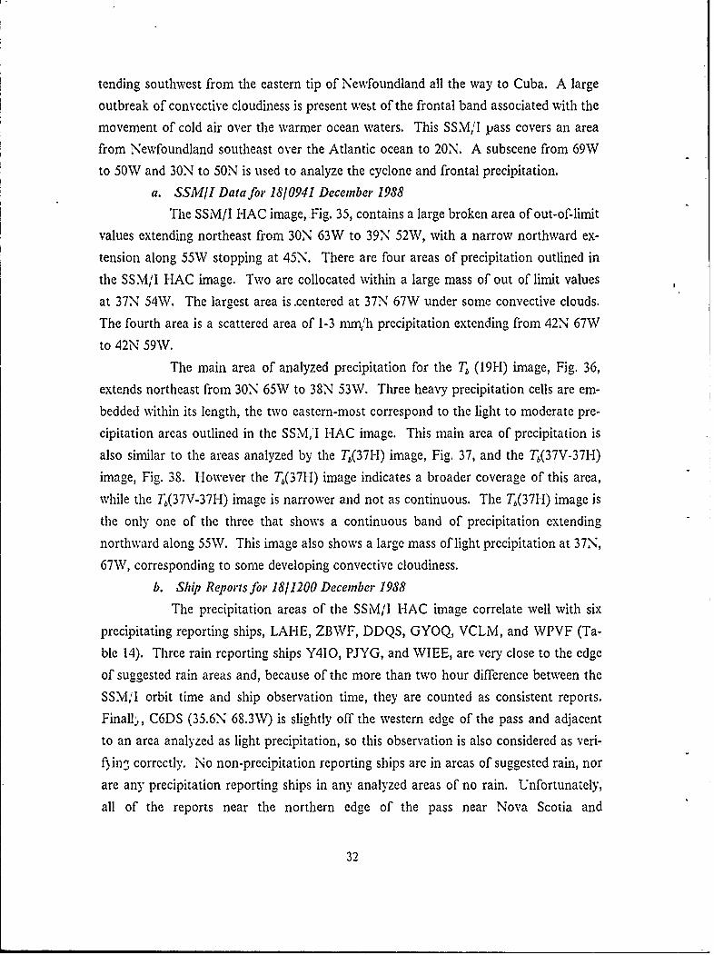
tending southwest from the eastern tip of Newfoundland all the way to Cuba. A large

outbreak of convective cloudiness is present west of the frontal band associated with the

movement of cold air over the warmer ocean waters. This SSM,1I pass covers an -area

from Newfoundland southeast over the Atlantic ocean to 20N. A subscene from-69W

to 50W and 30N to 50N is used to analyze the cyclone and frontal precipitation.

a. SSM/I Data for 18/0941 December 1988

The SSM/I HAC image, Fig. 35, contains a large broken area of out-of-limitvalues extending northeast from 30N 63W to 39N 52W, with a narrow northward ex-

tension along 55W stopping at 45N. There are four areas of precipitation outlined in

the SSM/I HAC image. Two are collocated within a large mass of out of limit values

at 37N 54W. The largest area is.centered at 37N 67W under some convective clouds.

The fourth area is a scattered area of 1-3 nim,'h precipitation extending from 42N 67W

to 42N 59W.

The main area of analyzed precipitation for the T (19H) image, Fig. 36,

extends northeast from 30N 65W to 38N 53W. Three heavy precipitation cells are em-

bedded within its length, the two eastern-most correspond to the light to moderate pre-

cipitation areas outlined in the SSMI HAC image. This main area of precipitation is

also similar to the areas analyzed by the T(37H) image, Fig. 37, and the T5(37V-371-1)

image, Fig. 38. However the T(3 7H) image indicates a broader coverage of this area,

while the T(37V-37H) image is narrower and not as continuous. The T(37H) image is

the only one of the three that shows a continuous band of precipitation extending

northward along 55W. This image also shows a large mass of light precipitation at 37N,

67W, corresponding to some developing convective cloudiness.

b. Ship Reports for 18/1200 December 1988The precipitation areas of the SSM/I HAC image correlate well with six

precipitating reporting ships, LAHE, ZBWF, DDQS, GYOQ, VCLM, and WPVF (Ta-

ble 14). Three rain reporting ships Y410, PJYG, and WIEE, are very close to the edgeof suggested rain areas and, because of the more than two hour difference between the

SSM,1 orbit time and ship observation time, they are counted as consistent reports.

Finall,, C6DS (35.6N 68.3W) is slightly off the western edge of the pass and adjacent

to an area analyzed as light precipitation, so this observation is also considered as veri-

f in- correctly. No non-precipitation reporting ships are in areas of suggested rain, nor

are any precipitation reporting ships in any analyzed areas of no rain. Unfortunately,

all of the reports near the northern edge of the pass near Nova Scotia and

32

Newfoundland coasts are either within a 3' wide swath of missing data or are too close

to land to be used with any confidence.

The Tb(19H), T(37H), and the Tb(37V-37H) enhanced brightness temper-

ature images show LAHE and ZBWF, who are reporting rain, located within areas of

suggested rain. GYOQ, reporting intermittent showers is within rain areas for the 19H

and 37H channels only. VCLM and WPVF are either in reasonable proximity to rain

areas to verify as a consistent report or are actually analyzed within an area of suggested

rain. PJYG (37N 67W) and Y410 (42.4N 52.1W) are only analyzed correctly by the

Tb(37H) image. The three remaining rain reporting ships, DDQS, WIEE, and VCTG,

are located in non-rain areas for all three brightness temperature images. DDQS is lo-

cated to the north of a shower region for the Tb(37 H) image, so it is consistent with the

analyses. However, neither the T,(1 9 H) nor the T(37V-37H) images analyze showers in

the area. WIEE is located southeast of the frontal rain band for all three brightness

temperature images. Allowing for the time difference of two hours between the SSM,'I

orbit time and ship observation reporting time this is not a strong disagreement. The

last missed rain report is that of VCTG, but this ship is located just east of Nova Scotia

and is affected by the land, sea discrimination table within the SSM,'I channels. None

of the images show rain areas analyzed over non-precipitating ship reports. The re-

maining six non-precipitating ship reports are within areas of no precipitation in all three

brightness temperature images.

33

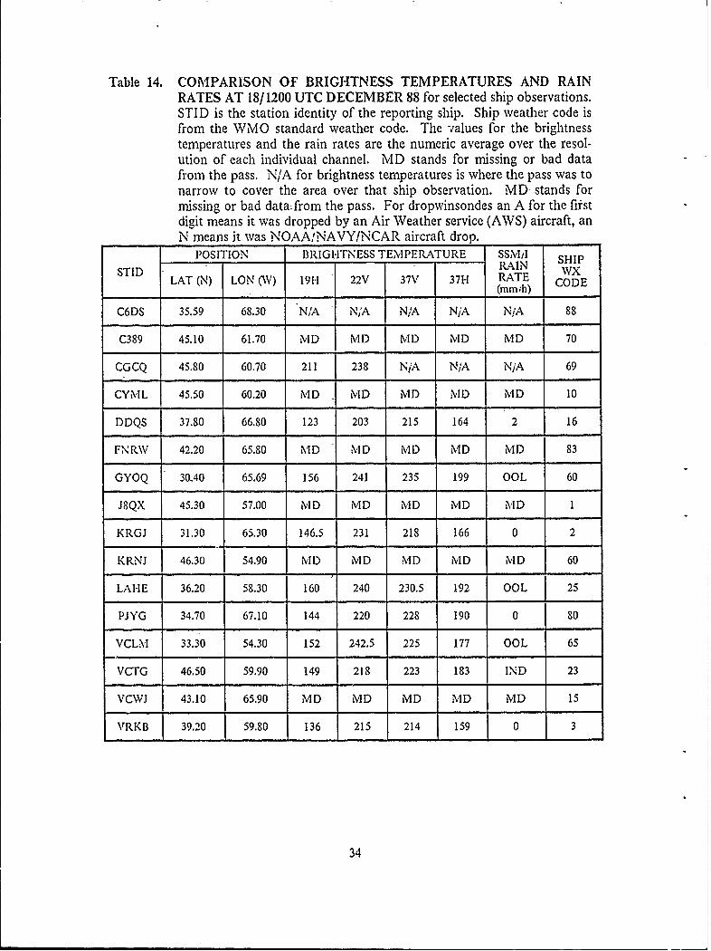
Table 14. COMPARISON OF BRIGHTNESS TEMPERATURES AND RAINRATES AT 18/1200 UTC DECEMBER 88 for selected ship observations.STID is the station identity of the reporting ship. Ship weather code isfrom the WMO standard weather code. The values for the brightnesstemperatures and the rain rates are the numeric average over the resol-ution of each individual channel. MD stands for missing or bad datafrom the pass. N/A for brightness temperatures is where the pass was tonarrow to cover the area over that ship observation. MD- stands formissing or bad data- from the pass. For dropwinsondes an A for the firstdigit means it was dropped by an Air Weather service (AWS) aircraft, anN means it was NOAA/NAVY/NCAR aircraft drop.

POSITION BRIGHTNESS TEMPERATURE SSMII SHIPSTID RAIN WX

LAT (N) LON (W) 191-1 22V 37V 37H RATE CODE

(mmih)

C6DS 35.59 68.30 N/A N'A N/A NiA N/A 88

C389 45.10 61.70 MD MD MD MD MD 70

CGCQ 45.80 60.70 211 238 N/A N/A N/A 69

CYblL 45.50 60.20 MD MD MD MD MD 10

DDQS 37.80 66.80 123 203 215 164 2 16

FNRW 42.20 65.80 MD MD MD MD MD 83

GYOQ 30.40 65.69 156 241 235 199 OOL 60

J8QX 45.30 57.00 iD iD MD MD MD I

KRGJ 31.30 65.30 146.5 231 218 166 0 2

KRNJ 46.30 54.90 MD MD MD MD MiD 60

LAIE 36.20 58.30 160 240 230.5 192 OOL 25

PJYG 34.70 67.10 144 220 228 190 0 80

VCLM 33.30 54.30 152 242.5 225 177 OOL 65

VCTG 46.50 59.90 149 218 223 183 IND 23

VCWJ 43.10 65.90 MD iD MD MD MD 15

VRKB 39.20 59.80 136 215 214 159 0 3

34

VYSV 44.80 66.69 MD MD MD MD MD 22

WIEE 32.09 56.80 145 234 218 163 0 20

WPKD 39.20 58.10 139 222 215 163 0 1

WPVF 36.80 53.90 140.5 220 221 172.5 OOL 60

WWPI 35.90 63.40 139 222 220 175.5 0 0

XCSG 42.30 55.80 152 227 227.5 193 0 1

Y410 42.40 54.10 135.5 225 213 156 0 62

YWD6 40.50 68.10 115 191.5 205 145 0 2

ZBWF 37.59 53.50 197 254.5 252 238 1 82

N081 42.21 63.07 MD MD MD MD MD

N082 41.26 62.15 133.5 205 211 157 0

N085 39.69 60.65 135 211 213 163 0

35

V. SUMMARY AND CONCLUSIONS

SSM/I rain rate estimates have been investigated for two periods of cyclogenesis

observed by the ERICA project. Four precipitation analysis methods were studied, (1)

the current SSM/I HAC algorithm, (2) the Spencer et al (1989) 85 GHz polarization

diflerence (PCT), (3) enhancements to the T (19H) and T(37H) brightness temperature

images and, (4) the T( 37) GHz polarization difference. Ship, coastal radar data and

dropwinsonde soundings for the closest reporting period to each orbit were used to val-

idate the images in each IOP.

There is considerable uncertainty in the interpretation of the HAC rain rate algo-

rithm. Specifically, large out-of-limits rain rate areas occur in the vicinity of wintercyclones. This was a common occurrence for mid-latitude winter data examined in this

study. The study of the SSM,'I HAC rain rate has indicated the out-of-limits areas occur

where the rain flags indicate rain (i.e. when T,(19H) greater than 160 K, or when

T(37V-37H) is less than 30 K) yet the rain rate calculated from the regression equations

is less than zero. One approach for the display of the HAC data would be to treat the

out-of-limit classification as no rain. The data analyzed in this thesis suggests this ap-

proach would eliminate significant areas of light precipitation. A second approach

would be to reclassify the out-of-limit values as light precipitation and this approach

would be the preferred short range solution.

The areas of light-moderate precipitation, 1-8 mm,,h, analyzed by the HAC data do

compare well with ship, radar data and the dropwinsonde soundings. Although the

overall areas designated as light and moderate precipitation by the HAC data is small,

relatiN e to the large out-of-limits area, they accurately depict regions of rain. The SSM,,I

HAC data also does well in analyzing shower activity and isolated cells of moderate to

heavy precipitation. The PCT images, studied in IOP 2, were extremely noisy and,

therefore, difficult to interpret. However, the areas of suggested precipitation were lo-

cated in close vicinity to convective and heavy precipitation areas. The amount of noise

in the 85 GHz image prevented a more detailed analysis.

The enhanced T(19H) and T(37H) GI-Iz provided alternative, useful rain-no rain

analyses. The T( 37H) is found to be better at mapping total rain areas. In particular,

the T(37H) with its higher resolution resolves post-frontal shower activity which is not

resolved by Tb(19H) channel. Also, the T(37H) channel has better sensitivity to light

36

rain areas than the T(1 91-I). The T(37H)'s warmer temperature enhancements appear

to overestimate the extent of moderate and heavy precipitation areas. The threshold

temperature of 220 K for the heaviest rain should be increased to 245 K. For improved

heavy precipitation analysis, the T(19-1)- channel should be used. The Tb(37V-37-I) in-

dicates the smallest regions of precipitation areas. The rain/no rain flag of 30 K appears

too low and should be revised upward.

The rain,'no rain comparisons between the ship observations and the four different

brightness temperature channels from the five SSM,1I orbits studied in IOP 2 and 3 have

been summed and are presented in Tables 15, 16, 17, 18, and 19. Tables 15 and 16

summarize the SSM,I HAC results. The out-of-limits areas are handled two different

ways in the tables. In Table 15, the out-of-limit area is assumed to be no rain, while

Table 16 uses these areas as rain. Comparing these two tables it is evident that over

twice as many ship rain reports are correctly identified when the out-of-limit areas are

considered as precipitation regions. Although the no rain ship reports classification is

slightly less successful, the overall percentage of correct reports increases by 16%o, from

61% to 77%. The out-of-limit areas appear to be reliable estimates of rain, but a major

problem is the regression estimates of negative rain rates. New regression equations are

urgently needed to eliminate this out-of-limits category. For now, labeling of the out-

of-limit values as light rain, 1-3 mmh, would be a reasonable approach, which is sup-

ported by the results in Table 16.

Table 15. RAIN/NO RAIN STATISTICS FOR THE SSM/I HAC IMAGE whenOOL values are considered to be no rain.

"" SHIP AND DROPWiNSONDE OB-

SSM/I VS SHIP OBSERVATIONS SERVATIONSRA IN NO RAIN

SSMI 1HAC IM- RAIN I IAGE NO RAIN 26 32

37

Table 16. RAIN/NO RAIN STATISTICS FOR THE SSM/I HAC IMAGE whenOOL values are considered to be rain values.

SHIP AND DROPWIN!\SONDE OB-

SSM/I VS SHIP OBSERVATIONS SERVATIONSRA IN NO RA IN

SSMII IAC FM- RAIN 24 3AGE NO RAI N 13 30

Tables 17, 18, and 19 describe the comparison between ship and dropwinsonde re-

ports and the T(19H), T(37H), and T(37V-37H) channel enhanced brightness temper-

ature images. From Tables 17 and 18, it can be seen that they both have a better

percentage of correct reports, 74% and 71%, respectively, than the SSM,'I HAC image

excluding the- out-of-limits areas. The T,(37V-37H) brightness temperature image does

the poorest of the three enhanced brightness images, with only 64% of the ship and

dropwinsondes correctly analyzed. However, even with this lower percentage it is still

slightl better than the basic SSM;I HAC image. This channel does better than all the

others in analyzing areas of no precipitation over ships reporting no rain, but did not

successfully analyze the rain reporting ships, missing two-thirds of them.

When the out-of-limits areas are classified as rain, the statistics from the I-AC (Ta-

ble 16), T(19H) and T(37H) are comparable. The classification of no rain ships is quite

successful. The major difficulty appears to be the classification of rain reporting ships

as no rain. Most of this is attributable to two causes: (1) the time difference between

the SSM, I pass and the ship reporting times (over 2h for the worst case), and (2) the

intermittent or shower type weather reported by the ships. Approximately 50% of the

rain reporting ships classified as no rain by all the methods is due to the intermittent or

shower type weather reported, while only 15%, of the missed rain reporting ships is due

to the time difference between the SSM/1 pass and the ship reporting time.

There were a total of 12 moderate to heavy rain reports for this data period. The

Tb(37I-I) analyzed nine correctly, the T (191-I) correctly analyzed eight, while the

T(37V-37H) images only interpreted seven correctly. The SSM, I HAC images were able

to correctly analyze seven, with tmo analyzed in out-of-limits areas. Therefore, all the

enhanced brightness temperature images were as successful as the basic HAC image at

analyzing the moderate to heavy rain reports.

38

Table 17. RAIN/NO RAIN STATISTICS FOR THE Tb (19H) IMAGES1H1P AND DRoPWINSOND3E OB-

SSM/I VS SHIP OBSERVATIONS SERVATIONSAIN NO RAIN

T (19H) IMAGE RAIN T FNO RAIN s 35

Table 18. RAIN/NO RAIN STATISTICS FOR THE T (37H) IMAGESHIP AND DROPWINSOINDE OB-

SSM,:I VS SHIP OBSERVATIONS SERVATIONSRLA I NO RAIN

T(3111 AERAIN 120 4

ITF(37H IAGI~I

NO RAINt t i 33

Table 19. RAIN/NO RAIN STATISTICS FOR TheE Tb (37V-37or n) IMAGESIP1 AND DROPWINSONDE OB-

SSM na VS SHIP OBSERVATIONS SERVATIONSRA INo NmO RAIN

T (37H) IMAGERAN11NO RA IN 26 36

From this study it is obvious that the four channel SSM,'I HAC regression algo-

rithm, in its current form can not satisfactorily analyzete the operational precipitation.Using a single or dual channel measurement appears to give similar results. Until a

better precipitation algorithm is devised, enhancements of the basic channel imageswould provide valuable information for the operational meteorologist.

Recommendations for future study include studying more SS.M,'I passes within the

remaining ERICA IOP's. Hopefully, SSM, I data over fullb mature cyclone centers can

be obtained to more accurately determine how the SSM, I HAC regression algorithm

resolves heav rainfall. Further stud is needed to determine if the regression approach

can be used to estimate precipitation areas, particularly in light precipitation areas. The

best method of SSM, I verification would be with aircraft radar data at the same timeas the satellite pass. Numerous flights by the NOAA P-3 radar-equipped aircraft were

39

made during ERICA. The intercomparison of radar and SSM/I data would provide an

exciting data base to develop new SSM/I rain rate algorithms.

40

APPENDIX A. SATELLITE PRECIPITATION ESTIMATION FIGURES

165mod heavy

29 5St emper a tur e) 1 ight mod

K t247.5

.92 .9 10 .0

UIs(albedo)

Fig. I. Two dimensional precipitation histogram using GOES IR and VIS digitalsatellite data. [After Sheridan (1988).)

41

-- Sotellite rain2-0- Radar rain

0.5.

2 Iep 4 *p Se 9 ep

Fig 2. Saelt ranrtessrda anrt.[fe Stu eta 199.

42 * I

10 20 30 40 50 60

VOLUME/3 -SCATTERING 8.

WATER/--- ICE /

E/

/ 19.35

Fig. 3. M4ie volume scatterini, coefficients for a M1arshall-Palmer precipitation sizedistribution of water and ice spheres at three frequencies (GIIZ). (Aftici Kidder andVonder Hlarr (1990).]

43

VOLUME3 ABSORPTION

WATER-iCE

2- 25.

(E

191

0

Fi g. 4. Volume absorption cocfficients for a imarsliall-Palmcr precipitation sizedistribution of water and ice spheres at tlrce frequencies (GlIZ). [After Kidder andVonder 1-Iarr (1990).]

44

1.0

- 0.8 3

20. 6

0.43

0.2WAE

0 10 20 30 40 50 60RAIN RATE (mm/h)

Fig. 5. Single scattering albedos for a Marshall-P~almer precipitation size distrib-ution of water and ice spheres at three frequencies (GI-Z). [After Kidder andVondcr Hlarr (1990).]

45

280 - OCEAN- LAND

260

240-1 118 GHz

220J

200

TB (K)R (" I I37 GHz180 1

1606

140 1

12

85.6 GHz100-

801 L ,10 20 30 40 50 60

RAIN RATE (mrrdh)

Fig. 6. Brightness temperature versus rain rate. [After Kidder and Vonder Hlarr(1990).]

46

26019

-S 37

~230-(9w H

1200-

uJ0-

W, 170-

wz

co 140

0 10 20

RAIN RATE (mm/hr)

Fig. 7. Mid-latitude occan brightness temlperature veisus rain rate at 19 and 37Gl-z. [After Hollinger ct al (1987).]

47

APPENDIX 13. CASE STUDY OF IOP 2

....... :;. . .

.sit

Fig. 8. GOES infrared cast coast U.S. sector imagery for 12/2301 December 1988.

48

-

Fi g. 9. SSM\, 1 H AC pincipitatio 1I image at 12:2303 December 1988. For colorcodle values see tabe 5.

49

Fic. 10. SSM I 19H- GHz brightness temperature imagea 21133Dcme19SS. For color code values see table e9t1.20 ecme

so

Fig. 11. SS.M:I 37H GHz brightness temperature image at 12,12303 December198S. For color code values see table 7.

Fie. 12. SSNJ I 37V -371-1 Gl-z brightness temperature image at 12:2303 De-cember I9SS. For color code values see table S.

52

Fig.- 13. PCT brightness temperature image at 12:12303 December 19S8. For colorcode values see table 6.

53

400

YEK2PEBO

NJPX*KRPO

; ~NYWL WGWC

ss - WDi 70 0

rVD B G- 300

000 TW1PECMER8

Fi.14 eahr an a fr13000Dcebr 98.Wate0smol1rfrm heWM sanar watercoe abe.Th sli lneouliesth aeaoOOLvales,~vhle hedased ineoutinS eae franls hn 5im'r

54

................ .....

4C' ----------- ~ .....

4 ,

.. .........

Fig. 15. GOES infrared east coast U.S. sector imagery for 13/2301 UTC Decem-ber 1988.

55

Fi.16. SSNI I HAC precipitation image at 13:2257 December I9SS. For colorcode values see table 5.

Fig. 17. SSN.IA 19H GHz brighltness temperature image at 13;2257 December19SS. For color code values see table 9.

F-g. IS. SSM I 171-1I Qla brightness tcwperature zmiage at 13.22i7 December19 S. For color code, values see lab!%,7

Fiki. 19. SSMIl~ 3V - 37H GIiz brightness tempe.rature image at 131,2257 De-

cember 19SS. For color code values see table 8.

59

Fia. 20. PCT briahtness temperature image at 13,12257 December 1988. For colorcode values see table 6.

60

N 00

N002 600

I \ KRPD

0YEI DHRG____________CGWS-

SC696~

CGA7 a

SKSYP-'

S775 I'-

A2300

A235

0000 UTC 14 DECEMBER 88

Fig.21. Weaherraini map for 14/0000 December 1988. Weather symbols areFom the WMOhe stnad weather code table. The solid line outlines the area ofOOL values, while the dashed line outlines the area of rain less than 15 mm/h11r.

61

APPENDIX C. CASE STUDY OF IOP 3

Fig. 22. GOES infr-ared east coast U.S. sector i-- -cry for 16,/223 1 Deccember1988.

62

A-

Fig. 23. SSNL I HAC precipitation image at 16,2220 December 19SS. For colorcode values see table 5. Latitude and lon~gitude lines are 10' apart with the southlatitude, of 20N and the western lonaitude of 70W.

63

Fig. 24. SSKII 191-1 G0Hz brightness temperature image at 16;,2220 Dcember19ss.

6.4

Fig. 25. SSM/l 3- 37H1 GlIz brightness temperature image at 16,2220 De-cember 1938.

65

Fig. 26. SSM,'I 311 Gl-z brightness tcrapcraturc image at 16,2220 Dcember

1988.

/WML

-- I 800/

A2 A11 24 - 0)I

0000 Ui ZIT DECEMBER 88

LEGEND

BROKEN AREA OF - SOLID AREA OF ---- BROKEN AREA OFOUT OF LIMIT VALUES -OUT OF LIMIT VALUES ---- LIGHT RAIN

Fig. 27. Weather rain map for 17/0000 December 1988. Weather symbols arerom the WMVO standard Weather code table.

67

Kt

bcr 1988. GOE izffrai'cd cst coast U.S siaryfr1,21UC )c-

ire,

Fie. 29. SSNI I HAC precipitation image at 17.2208 December 1988. Loneitudelines are 10' anart. with the western most loncitude 70W. For color code values seetable 5.

Fig. 30. SSI1 1911 GFW17 brightness temperature irnagc at 17/'2208 Dcemrber1983. Grey scale is same as that of figure 26.

70

-Pr

Fig. 3 1. SSMiI 371-1 Gl-z brighitness temnperature image at 17/2208 December1988. Grey scale is same as that or figure 24.

7'

Fig. 32. SSMI 37V -371- Gl-z brighuicss tcmlperature image at 17il20 D~e-ccmber 19SS. Grey scale is samec as that of figure 25.

72

I I,

00 '60

550S720 VxCSG - 400GHZK _9 -N214 A222

u .-S500

S840 N20 GUOI WPKD 4 X6ID

- *WWPIj L ENjR PJYG .- LH

DOS JKRH-G/ ____ ______

D- -C6DS I

/ */ LAHO

300 ~ 7j500~, ______ 300

* _____-KRGJ --~--

0000 UTC 18 DECEMBER 88

LEGEND

____BROKEN AREA OF -SOLID AREA OF....OUT OF LIMIT VALUES ---- LIGHT RAIN

SOLID AREA OF p7 AREA OF INDETERMINATEOUT OF LIMIT VALUES tZ.JVALUES

Fig. 33. Werather rain map for 1000Deccmber 1988. Weather symbols arcfromn the WMO0 standard wecather code tabic.

73

* .. .......... ..... ... .. ... ... .

7< 1.......... ....... ~

I M v-.. i.'-

Fig. 34. GOES infrared east coast U.S. sector imagery for 18/0901 UTG Dcem-ber 1988.

74

r-

Fig. 35. SS.M:I HAC precipitation image at 18:0941 December 1988. For colorcode values see table 5. Latitude lines are 10° apart with the southern most latitude20N.

75

Fig. 36. SSM/I 1911 Glz brightness temperature image at 18,10941 Dcemiber

1988. Grey scale is the same as that of figure 26.

76

Fig. 37. SSM,'1 371-1 G0Hz brightness temperature image at 18,0941 Decemnber198S. Grey scale is the same as that of figure 24.

77

Fig. 38. SSM/I 37V -371- Glilz brightness temnperature image at 18110941 Dc-cember 1988. Grey scale is the same as that of figure 25.

78

4iVCTG <RJ 1CG;CO ~'CYML

978 JO

/

700 VCW 600 wo

*N0*81 X6Sd Y 410

':?FNRWtJ8

YdD6

N6851 ..f-

VRKB WPKD

DDOS v -

.1 '--- WVF

V ~- ~ wp LAI-E '/

C6DS z______PJYG/ *

700 600 .V (' m VC

,* *')!10/ WIEE'

IKRGj /

-GYOO - 300

1200 U TC 18 DECEMBER 88

Fig. 39. Weather rain map for 18/1200 December 1988. Wcadhcr symbols arefrom the \VMO standard Nvcathicr codc table. The dash, dot line outlines brokenarcas of OOL values, whilc the dashed Jinc outlines solid areas of rain less than 15rrun/hr.

79

APPENDIX D. WMO WEATHER CODE TABLE

0,10 01 02 03 04 05 06 07 08 09

10 11 12 13 14 15 16 17 18 19__ - --__ -_-.1- . ___________

20 21 22] 23 24 (_J 25 26 *127 A] 281 29 RI.. If~f.. . - - - - 'fll'.i 4 iiP l ai~~ d.. -t , a . ,I*. r .. . - d* . S.All .. 4I

3 0 1 3 3 334 5 3 + 3 7 + 3 8 1+ 3

40 41 42 43 44 45 46 47 48 49

.,.P::.:.i .: , _. .... .. .... , , OV ' - -,

50 51 52 53 54 55 56 57 58 591 il 1 1 21 (111 1 I

.l ll ..... ,....,lt .#a.l . bUTli I . .. #..I. I--fl . la '70 * I.l4A) i 7. . M.. 0.A.... - 0 . i.. ... I

60 61 62 63 64 65 66 67 68 690 0 I..1 C*-

........ . .. .... . ..... ... ..,'__;______ . .... ___..........__....._ i;j *. ,., a.... .a

70 71 72 73 74 75 7G 77 78 79-* *-1 - --- --

!"£ ... . . . .- .- *... y.bv 4 k A S.80 * 82 83 84 85 86 87 88 8 9 A,

0V 9 9" .. ... .. .... . . . . i . . .. .. . . ! 1...

19, ] 395 96 98

Fig. 40. The Standard WMO Codcs

80

LIST OF REFERENCES

Barrett, E.C., and D.W. Martin, 1981: The use of satellite data in rainfall monitoring.Academic Press, London, UK, 340 pp.

Chalfant, A.E., 1989: Dynamics of an ERICA cyclone. M.S. Thesis, Naval PostgraduateSchool, Monterey, CA, 56 pp.

Griffith, C.G., W.L. Woodley, S. Browner, J. Teijeiro, M. Maier, D.W. Martin, J. Stoutand D.N. Sikdar, 1976: Rainfall estimation from Geosynchronous satellite imageryduring daylight hours. NOAA Tech. Rep. ERL 356-WMPO 7, Boulder, CO, 106pp.

------, W.L. Woodley, P.G. Grube, P.W. Martin, J. Stout, and D.N. Skidar, 1978: Rainestimation from geosynchronous satellite imagery-visible and infrared studies. Mon.,1ea. Rev., 106, 1153-1171.

Hadley, R., and C.W. Kreitzberg, 1988: The experiment on rapidly intensifying cyclonesover the Atlantic (ERICA) field study: objectives and plans. Bull. Amer. Meteor.Soc., 69, 1309- 1326.

Harnett, E., G. Forbes, and R. Hadlock, 1989: Experiment on rapid intensification ofcyclones over the Atlantic (ERICA) field phase summary. Department of Physicsand Atmospheric Science, Drexel University, Philadelphia, PA, 300 pp.

Hollinger, i., R. Lo, G. Poe, R. Savage, and J. Peirce, 1987; Special sensormicrowave;imager user's guide, Naval'Research Laboratory. 120 pp.

Katsaros, K.B.. 1. Bhatti, L.A. McMurdie, and G.W. Petty, 1989: Identification of at-mospheric fronts over the ocean with nicrowa e measurements of water vapor andrain. Wea. and Forecasting, 4, 449-460.

Kidder, S., and T. Vonder Harr, 1990: Principles of satellite meteorology. AcademicPress, New York, NY, in printing.

Liljas, E., 1984: Processed satellite images for operational forecasting. SwedishMeteorological and Hydrological Institute, Morrkoping, Sweden, 43 pp.

Scofield, R.A. and V.J. Oliver, 1977: A scheme for estimating convective rainfall fromsatellite imagery. NOAA Technical Memorandum NESS 86, Washingtion, DC, 47pp.

Sheridan, T.F., 1988: Satellite precipitation analysis for a developing North PacificOcean cyclone. M.S. Thesis, Naval Postgraduate School, Monterey, CA, 72 pp.

Spencer, R.W., 1I.M. Goodman, and R.E. Hood, 1989: Precipitation retrieval over landand ocean with the SSM, I: Identification and characteristics of the scattering sig-nal. J. Amos. Ocean Tech. 6, 254-273.

81

Stout, J.E., D.W. Martin, and D.N. Skidar, 1979: Estimating GATE rainfall withgeosynchronous satellite images. Mon. Wea. Rev. 107, 585-598.

Wash, C.H., L.A. Spray and L.C. Chou, 1985: Satellite cloud and precipitation analysisusing a minicomputer. NPS-63-85-003, 90 pp.

Wilheit, T.T., J.S. Theon, W.E. Shenk, L. Allison and E.B. Rodger 1976: Meteorologicalinterpretations of the images from the Nimbus 5 electrically scanned microwaveradiometer. J. Appi. Meteor., 15, 166-172.

----, A.T.C. Chang, 1980: An algorithm for retrieval of ocean surface and atmoshpericparar-;ters from the observations of the Scanning Multichannel MicrowaveRadiometer (SM MR). Radio Science., 15, 525-544.

Woodley, W., C.G. Griffith, J.S. Griffith, and S.C. Stromatt, 1980: The inference ofGATE convective rainfall from SMS-1 imagery. J. Appl. Meteor., 19, 338-408.

82