1

Evaluation of the NASA GISS Single Column Model Simulated Clouds Using Combined

Surface and Satellite Observations

Aaron D. Kennedy, Xiquan Dong, and Baike Xi

Department of Atmospheric Sciences, University of North Dakota, Grand Forks, ND

Patrick Minnis

NASA Langley Research Center, Hampton, VA

Anthony D. Del Genio and Audrey B. Wolf

NASA Goddard Institute of Space Studies, New York City, NY

Mandana M. Khaiyer

Science Systems and Applications, Inc., Hampton, VA

Corresponding author address: Mr. Aaron Kennedy, The Department of Atmospheric Sciences,

University of North Dakota, 4149 Campus Road, Box 9006, Grand Forks, ND 58202-9006.

Email: aaron.kennedy@und.nodak.edu. Phone: 701-777-4478.

2

Abstract

Three years of surface and Geostationary Operational Environmental Satellite (GOES) satellite

data at the Department of Energy Atmospheric Radiation Measurement (ARM) Southern Great

Plains (SGP) site are used to evaluate the NASA GISS Single Column Model (SCM) simulated

clouds from January 1999 to December 2001. The GOES derived total and high cloud fractions

for both 0.5o and 2.5o grid boxes are in excellent agreement with surface observations,

suggesting that ARM point observations can represent large areal observations. Compared to the

ARM observations, the SCM simulated most mid-level clouds, overestimated low clouds (8%),

and underestimated total and high clouds by 6% and 12%, respectively. To examine the

dependence of the modeled high and low clouds on the synoptic pattern and large-scale variables

such as relative hunmidity (RH) and pressure vertical velocity (omega), North American

Regional Reanalysis (NARR) data are included. The sucessfuly modeled and missed high clouds

are primarily associated with a trough and ridge upstream of ARM SGP, respectively. The PDFs

of observed high and low occurrence as a function of RH reveal tha thigh clouds have a

Gaussian-like distribution with mode RH values of ~50%, whereas low clouds have a gamma-

like distribution with the highest cloud probability occurring at RH ~ 80-90%. The PDFs of

modeled low clouds are similar to those of observed ones, however, for high clouds the PDFs are

shifted to higher RH than observed which results in a negative bias of high clouds because many

are observed below the specified stratiform paramterization threshold RH of 60%. Observed

clouds are well correlated with RH and omega fields, especially in the upper troposphere.

Modeled clouds are primarily correlated with low-level RH and 300-hPa vertical motion. While

ARM forcing and NARR RH fields are similar to each other, significant differences exist for

omega.

3

1. Introduction

Clouds are one of the most important elements in the Earth’s hydrology and energy

cycles, acting particularly through precipitation processes (Del Genio et al. 2005a) and the

Earth’s radiation budget. Their treatment in weather forecast and climate models is a significant

source of error and uncertainty (Gao and Li 2007; Cess et al. 1996; Randall et al. 2006).

Although considerable uncertainty still surrounds cloud feedbacks in General Circulation Models

(GCMs), one can assume that to reasonably simulate future climate, these models should be able

to accurately reproduce the current climatology of all clouds at a given location. Due to the

complexities of GCMs, the Single Column Model (SCM) approach was developed to evaluate

parameterizations (Randall et al. 1996) and has been implemented by the Atmospheric Radiation

Measurement (ARM) program (Ackerman and Stokes 2003) to improve the representation of

clouds and radiation in GCMs using long-term surface observations (Klein and Del Genio 2006).

SCM versions of GCMs typically have been used to simulate the atmosphere over limited

time periods, driven by field experiment data or enhanced soundings during intensive observing

periods (IOP, see JGR special issue, 2005). These exercises have proven difficult to interpret,

because model-data discrepancies can be due to inaccurate large-scale advective forcing,

inaccurate model physics, or problems with the cloud data, and instantaneous model errors may

not be climatically representative or diagnostic of problems with the model’s cloud feedback

(Del Genio et al., 2005b). Therefore, it is necessary to use a longer time series to have a

statisitically meaningful comparison.

Compared to observations from the International Satellite Cloud Climatology Project

(ISCCP; Rossow and Schiffer, 1999) and the Clouds and the Earth’s Radiant Energy Ssytem

(CERES, Wielicki et al. 1998; Minnis et al. 2008,2009), Zhang et al. (2005) found that the

4

majority of GCMs only simulated 30-40% of observed mid-latitude mid-level top clouds and

half of the GCMs underestimated low-level top clouds, however, not at a statistically significant

level. Limitations in the passive satellite data prevented a thourough analysis of high clouds.

To ensure that climate models reliably represent clouds, the parameterizations of cloud-

radiation-precipitation interactions and the associated heating and other feedbacks in the models

should faithfully represent what is found in nature. Therefore, the time-dependent frequency

distributions of cloud properties from the model should also be compared to those derived from

observations. Ultimately, improved cloud parameterizations can only result from an integrated

analysis of all available data sets, including long-term surface and satellite observations, single

column models, and reanalyses.

To provide a much-needed source of long-term cloud-radiation data for evaluating model

parameterizations, the ARM Program established the Southern Great Plains (SGP) site, centered

near Lamont, Oklahoma, in 1993. ARM has also included satellite observations to determine

cloud and radiative properties (Minnis et al. 1995, 2001) to complement the surface data, provide

large-scale averages, and bound the radiation budget at the top of the atmosphere (TOA),. In

addition to the surface and satellite measurements, Xie et al. (2004) developed the continuous

forcing product (1999-2001) over the SGP site. This product is often of a quality comparable to

that from Intensive Observing Periods (IOP) and has the advantage of being available for driving

SCMs over long periods (Del Genio et al. 2005b).

This paper reports on a continuous period of long-term surface and satellite observations,

SCM simulations, and their association with large-scale synoptic patterns and large-scale

variables provided by the North American Regional Reanalysis (NARR) over the ARM SGP

site. Although the evaluation of an individual SCM driven by a forcing dataset at one location

5

may have limited practical usage, the ARM SGP site is representative of a continental climate in

the mid-latitudes. This paper also investigates the seasonal and vertical variations of observed

clouds and their relationship to relative humidity and vertical motion which are widely used as

independent variables in GCM stratiform and convective cloud paramterizations in climate

models. The paper is formatted as follows. Section 2 gives a brief description of the different

datasets used in this study. In section 3, satellite and surface observed clouds are compared to the

SCM simulations on hourly, monthly, and seasonal timescales. SCM performance is

investigated within section 4 with the aid of large-scale parameters obtained from NARR and

ARM Forcing. Section 5 discusses and analyzes the seasonal and vertical variations of clouds

with relative humidity and vertical motion. Pertinent conclusions are summarized along with

plans for future work in the final section.

2. Datasets

Surface, satellite, ARM continuous forcing, and NARR reanalysis data sets have been

collected at ARM SGP during the period 1999-2001 for this study. Because the ARM continuous

forcing is required to run the GISS SCM and is only available during 1999-2001, model results

are compared with both surface and satellite observations for this 3-yr period. Both the surface

and satellite data sets are averaged into hourly means to match the SCM hourly temporal

resolution although their spatial resolutions are different.

a. Surface Observations

The DOE ARM 35-GHz Millimeter Wavelength Cloud Radar (MMCR) has a minimum

detectable reflectivity factor (Z) of -55 dBZ at 1 km and -35 dBZ at 10 km (Moran et al. 1998).

The MMCR operates at a wavelength of 8 mm in a vertically pointing mode and provides

6

continuous profiles of radar reflectivity from hydrometeors moving through the radar field of

view (FOV), allowing the identification of clear and cloudy conditions. The beam width is 0.2°

which results in a horizontal resolution of ~40m at 12km AGL. Cloud-top height (Ztop) is derived

from MMCR reflectivity profiles with an uncertainty of 90 m. The lowest cloud-base height

(Zbase) is derived from a composite of Belfort laser ceilometer, Micropulse Lidar (MPL), and

MMCR data (Clothiaux et al. 2000). Inclusion of the lidar allows for the filtering of insects

which produce a significant reflectivity during the spring and summer seasons over the ARM

SGP. Another source of error in the cloud radar retrievals is attenuation during precipitation

events, which leads to underestimated cloud top heights. To mitigate this issue, only

precipitation-free times are considered. This is expected to cause a negligible amount of

negative bias to cloud fractions derived for all levels; only 1.4% of all 5-minute samples

recorded precipitation.

The cloud fraction (CF), derived from the upward-looking narrow FOV radar-lidar pair

of measurements, is simply the percentage of returns that are cloudy within a specified sampling

time period, i.e., the ratio of the number of hours when clouds were detected to the total number

of hours when both radar and lidar/ceilometer instruments were working.

b. Satellite Observations

The satellite cloud products (Minnis et al., 2001) were retrieved using algorithms

developed for the NASA Clouds and Radiant Energy System (CERES) project. Cloud properties

were retrieved from half-hourly, 4-km 0.65, 3.9, 10.8 (infrared, IR), and 12.0-µm radiances taken

by the eighth Geostationary Operational Environmental Satellite (GOES). Cloudy pixels were

identified using an adaptation of the method described by Minnis et al. (2008a). The Visible

7

Infrared Solar-Infrared Split-window Technique was applied during daytime (solar zenith angle

< 82°) and the Solar-infrared Infrared Split-window Technique (SIST) was used at night (solar

zenith angle >82o) to derive cloud properties for those pixels (Minnis et al. 2009). The areal

fraction of clouds (instantaneous cloud amount from the satellite FOV) is the ratio of the number

of pixels classified as cloudy to the total number of pixels within a specified area (0.5ox0.5o in

this study). The primary technique for determining effective cloud height (Heff) is to estimate

effective cloud temperature (Teff) based on the 10.8-µm radiance adjusted to account for cloud

semitransparency first, and then to define Heff as the lowest altitude having Teff from a vertical

temperature profile based on a sounding or a numerical weather prediction (NWP) model

analysis. In this case, the algorithm uses atmospheric profiles obtained from the Rapid Update

Cycle 2 (RUC-2; see Benjamin et al., 2004) analyses. The profiles are altered at altitudes below

the 500-hPa level using a lapse rate anchored to the 24-h running average surface temperature as

described by Minnis et al. (2009). This study uses the gridded layer-averaged GOES-8 cloud

amounts (Palikonda et al., 2006; data available at http://www-angler.larc.nasa.gov/). According

to the retrieved Heff, the GOES-derived clouds can be classified as low (<2 km), middle (2-6 km),

and high (>6 km) clouds. Total cloud coverage is simply the sum of the low, middle and high

cloud amounts determined from the GOES data.

c. NASA GISS SCM

The model analysis in this paper uses an archived run of the NASA GISS SCM that is

identical to the one described in Del Genio et al. (2005b). The model is based on the SI2000

version of the GCM, but with cloud and convection physics updates described in Del Genio et al.

(2005a). The SCM has 35 vertical layers and an implied horizontal resolution of 2°×2.5°

8

corresponding to a grid box of approximately 220 km square at the SGP. The continuous forcing

driving this SCM run uses constrained variable analysis with RUC-2 hourly analyses as the

background field (Zhang et al. 2001, Xie et al. 2004). These hourly analyses are constrained by

ARM surface and GOES-8 satellite observations to balance observed mass, momentum, heat,

and moisture budgets within the column. The model is run hourly from the observed advective

temperature and moisture tendencies and is reinitialized at the beginning of each day to remove

climatic drift (Del Genio et al. 2005a).

The SCM predicts cloud water but uses an RH-based scheme to diagnose large-scale

cloud fraction (Sundqvist et al. 1989, Del Genio et al. 1996) which requires a tunable threshold

relative humidity parameter, U00. Commonly set around 60%, stratiform clouds are not allowed

to occur below this value. Above this threshold, cloud amount (fraction) is assumed to increase

with grid box mean RH. U00 is held constant globally and vertically, and only varies (relative to

saturation over liquid water) when temperatures are colder than -35ºC to account for the

difference between saturation vapor pressure over ice rather than water. For this reason and also

because the convective scheme separately diagnoses a convective cloud cover, the SCM can

occasionally create clouds at values below the prescribed threshold (Del Genio et al. 1996). The

convective scheme uses mass flux and is closed by moving enough mass to neutralize cloud-base

instability (Del Genio and Yao 1993). This scheme allows for up to two convective cloud tops

(such as cumulus and cumulonimbus) and cirrus anvils by detraining \water vapor/condensate

from the convective scheme into the gridbox, where the subsequent evolution is handled by the

stratiform scheme.

d. North American Regional Reanalysis (NARR)

9

The NCEP North American Regional Reanalysis (NARR, Mesinger et al. 2005) is a

long-term (1979-2007) climate data set with 3-hr temporal, 32-km horizontal, and 45-layer

vertical resolutions over the North American domain. It contains outputs of all atmospheric

variables and fluxes, and it is nicely suited for diagnosis of synoptic and mesoscale conditions

over the ARM SGP site. NARR uses the operational NCEP ETA model and its 3D-VAR data

assimilation technique on a wide variety of observation platforms. The end result is a dataset that

improves in almost all areas over the earlier global reanalysis dataset.

3. Evaluation of the NASA GISS SCM Simulations

a. Methodology

Although the ARM radar-lidar observations provide the most reliable vertical

distributions for verifying the GCM simulations, large-scale satellite data are critical for

evaluating GCM simulated spatial distributions of clouds because they provide a means to

account for the scale differences between the SCM and surface site. Comparisons between the

ground- and satellite-based observations must be conducted carefully because of significant

spatial and temporal differences between the two different observing platforms. The differences

between the satellite and surface observations must be reconciled before those observations can

be used to validate the model simulations. For example, under what conditions are the surface

point observations representative of the large grid box of satellite observations? Xi et al. (2009)

have shown that there is excellent agreement in long-term mean CFs determined from the 10-yr

surface and GOES data. The CF is independent of temporal resolution and spatial scales, at least,

up to the size of a 2.5° grid box providing there are enough samples. Cloud frequency of

10

occurrence increases and mean instantaneous cloud amount decreases with increasing averaging

time and spatial scale.

The temporal, spatial, and vertical resolutions of surface radar-lidar and GOES

observations and SCM simulations are listed in Table 1. To have the same temporal resolution

for the three data sets, both the surface and GOES data sets have been averaged into hourly

means to match the SCM hourly outputs. Since GOES can provide only three levels (low,

middle, and high) of clouds, both surface (90-m resolution) and SCM (~25-hPa resolution)

vertical distributions of clouds have been binned into those three levels to make a reasonable

comparison. For spatial resolution, the 0.5°×0.5° grid box of GOES observations have been

extended into a 2°×2.5° grid box to match the SCM domain. Figure 1 shows an enlarged 2.5°

grid box including the percentages of area from each 0.5° grid box.

Satellite observations may include several error sources that can significantly impact the

derived instantaneous cloud amount. In particular, observational noise or retrieval errors can

lead to positively biased cloud frequencies for the 0.5° grid box because more clouds occur for

very small instantaneous cloud amounts (<5%). Figure 2a illustrates the hit rate (fraction of

hours during which satellite and radar observations agree) as a function of the instantaneous

GOES cloud amount threshold used here to discriminate between cloudy and clear scenes. The

impact of noise or retrieval errors is easily seen for low clouds where their hit rate increases to a

maximum at ~10% cloud amount and then is asymptotic to a hit rate of 0.8. This in turn impacts

the total cloud hit rate. This suggests that for the best agreement between radar and satellite

observations, a threshold instantaneous cloud amount must be set to discriminate between cloudy

and clear scenes on an hour-to-hour basis. Other than a minimum below 2%, hit rate slowly

decreases for high clouds. This indicates that setting a threshold too high would arbitrarily

11

classify correct retrievals of clouds by the satellite as clear. Except for optically thin cirrus,

satellites should detect most high clouds. Figure 2b demonstrates the impact of the prescribed

cloud amount thresholds on the GOES-derived CF. Small cloud amount thresholds alter the

derived cloud fractions by a negligible amount (less than 1%). To filter out GOES observational

noise and/or retrieval errors and to keep more cloud samples within the SCM domain, a threshold

of 5% GOES cloud amount was used to discriminate cloudy (≥5%) and clear (<5%) scenes in

this study.

To further investigate the 5% threshold, consider Fig. 3 which illustrates the frequencies

of GOES-observed (before applying the 5% threshold) and SCM-simulated cloud amounts. The

distributions of GOES cloud amount are characterized by being bimodal for high clouds and

exponentially decreasing for the low- and mid-level clouds. Note that the cloud amounts within

the first bin of all three levels are less than 5% and have been filtered out in this study. Even if

some of these scenes are realistic, the radiative impact of such a small cloud fraction is probably

minimal on climatic scales. Despite the large peaks in the first bin of Fig. 3, the distributions are

consistent with the Zhang et al. (2003) study which explored GOES cloud amount distributions

over a 9.5°×13.5° area centered on the ARM SGP during a summer month. Modeled three-level

cloud fractions peak at large cloud amounts (>85%) while others are nearly equally distributed

from 5% to 85%. This is most likely caused internally within the SCM cloud parameterization

scheme when volumetric cloud fraction is converted into the horizontal scale.

b. Cloud Fraction and Frequency

For the GOES results, the cloudy frequency of occurrence FREQ is taken to be 0 for

instantaneous cloud amount AMT < 0.05 and 1 when AMT ≥ 0.05. The monthly averaged AMT

12

is the average of all hourly AMTs (>0.05) and represents the averaged cloud amount when

clouds are present. The average FREQ (probability of cloud occurrence) is the ratio of the

number of times AMT>0.05 to the total number of satellite observations during that month.

Finally, the monthly mean CF is defined as the product of the monthly averaged instantaneous

AMT and FREQ. This is equivalent to the CF derived by the radar-lidar observations if clouds

occur uniformly over the domain. This assumption is valid at the ARM SGP on scales of

months, seasons, and years (Xi et al. 2009).

1) DIURNAL VARIATION OF CLOUD FRACTION

The diurnal variations of hourly mean total and three-level CFs are illustrated in Fig. 4.

The diurnal cycles are plotted in UTC (SGP local time=UTC - 6 hours) because the SCM was

reinitiated at 00 UTC every day with no spin-up period. For surface observations, diurnal

variations primarily occur for low clouds, which are typically subject to mesoscale or microscale

forcing with the rise/set of the sun. There are more low-level clouds in the morning than during

the afternoon. Very little variability occurs for clouds above 6 km which are more often tied to

large-scale forcing independent of the diurnal cycle. Other than anvil cirrus clouds due to

afternoon/evening thunderstorms, high-level clouds are often associated with the large-scale

forcing, such as ascent with baroclinic waves.

For GOES-derived CFs, there is no strong diurnal variation for total clouds, but there is a

significant drop for high clouds and an increase in both low and middle clouds around sunrise

(~12-13 UTC in Fig. 4). This is primarily due the effect of multilayered clouds on the different

retrieval algorithms used for day and night. The increased low and midlevel CF during daytime

is mainly due to the fact that high, thin cirrus over low clouds only slightly diminishes the IR

brightness temperature TIR, but the visible channel indicates that the cloud is optically thick. The

13

net result is that the VISST assumes that the Teff is essentially the same as TIR. Thus, the VISST

retrievals for thin-over-thick multi-layered cloud systems yield a low or midlevel cloud

depending on the altitude of the lower cloud and the optical thickness of the upper-level cloud. If

the upper-level cloud has an optical depth greater than about 3 or so, the cloud is interpreted as a

high cloud and the lower cloud is undetected. Even in single-layered cirrus cases, the cloud

height is underestimated (Smith et al., 2008) because the cirrus optical depth is overestimated

(Min et al., 2004).

At night, however, the SIST is relatively insensitive to the presence of a low-level cloud

underneath a thin high cloud because the surface and low-cloud temperatures typically differ by

only a few degrees. Thus, the upper-level cloud is detected as being semi-transparent and Teff

differs significantly from TIR and a relatively accurate high-cloud altitude results fro both single

(Smith et al., 2008) and multi-layered clouds. The low clouds underneath the cirrus are not

detected. If the upper-level cloud is optically thick, the underlying low and midlevel clouds will

not be detected Therefore, it is possible for GOES to miss some low-level clouds underneath

optically thin cirrus clouds during the nighttime and/or low clouds with similar brightness

temperatures as the ground. These algorithmic effects result in the high cloud CF decreasing

from nighttime to daytime, which corresponds to an apparent increase for low and mid-level

clouds. The low and midlevel cloud amounts are always less than the values from the radar

because of the screening effect of the high clouds.

The SCM simulated clouds monotonically increase from 00 UTC to local noon (~18

UTC) for total and all three-level clouds as shown in Fig. 4. The day (12 – 24 UTC) minus night

(0 – 12 UTC) cloud fractions differences vary by 28-37% depending on the level. Although

other issues cannot be completely ruled out, the culprit for this steady increase in CF is mainly

14

due to the 00 UTC daily initialization for the model. As might be expected, this model spin-up

time (~12 hours as shown in Fig. 4) would introduce a negative bias to all cloud fraction

calculations. Therefore, all CFs derived from surface, GOES, and SCM datas are based only

upon the 12 – 24 UTC time period.

2) SEASONAL VARIATION OF CLOUD FRACTION AND FREQUENCY

The monthly variations of total, high, middle and low cloud fractions and frequencies

derived from surface radar-lidar, 0.5o and 2.5o grid boxes of GOES observations, and SCM

simulations at the SGP site during the 3-yr period are illustrated in Fig. 5. Their corresponding

annual means are summarized in Table 2. Both the surface and GOES-derived total CFs agree

very well in general trend and magnitude with almost identical annual means. They both peak

during the January-March period, have a second peak in June, followed by a significant drop into

July, finally increasing from summer to winter. The monthly variations of the three-level CFs

basically follow the total CF trend with minor variations. Although the GOES-derived high CF

is 0.1 – 0.2 less than that from the surface, the high-cloud frequency agrees well with the surface

observations suggesting that at least part of the high cloud cover is correctly identified whenever

high clouds occur during the daytime. Middle and low CFs are less than the surface observations

throughout the year except for the July-August period. This is understandable because some of

the middle and low clouds are masked by upper level clouds. The fact that some of the low and

mid-level clouds are actually misidentified high clouds, as discussed above, is reinforced by their

greater frequencies of occurrence as seen by the satellite. Although these comparisons are not

long enough to represent a climatology of clouds over the SGP site, it is concluded that they are

15

typical because the seasonal variations of clouds in this study are very similar to other studies

that used longer time series (Dong et al. 2006, Xi et al. 2009).

Despite being consistently less than observations, the monthly variations of SCM-

simulated total and three level clouds undergo seasonal changes that are somewhat similar to

those observed from the surface and satellite with one exception. The SCM midlevel CF

maximum is several months out of phase with the others, however, still corresponds with a local

maximum in the observations. As seen in both Figs. 4 and 5, the SCM simulates significantly

fewer clouds overall (~10%) than detected by the observations regardless of the overlap

assumption used. Investigation of individual layers reveals that the SCM simulated most middle

and low cloud cover compared to the surface and GOES observations. The SCM underestimated

high clouds fractions relative to the surface data, but yields remarkably good agreement for high

clouds with no the no overlap assumption compared to satellite observation.

The monthly variations of cloud frequencies are nearly the same as their CF counterparts

except with relatively large values. As expected, the observed cloud frequencies are greater for

the large grid box (2.5°) than for the small grid box (0.5°) and ARM surface observations, i.e.,

the cloud frequencies increase with larger spatial scales. For high clouds, the 0.5° grid box of

GOES and radar observed cloud frequencies are nearly equivalent, which suggests that on the

order of an hour, radar observations are a good approximation for a 0.5° grid box of satellite

observations. The SCM simulated cloud frequencies are lower than observed ones except for

low clouds. For high clouds, the SCM frequency is nearly the same as the corresponding CF

(0.16 vs. 0.15), which indicates that the model simulated either clear skies or scenes with large

cloud amounts. This argument is also supported by Fig. 3a.

16

Table 2 summarizes the 3-yr averaged cloud fractions and frequencies for total and three-

level clouds. The percentages of surface and GOES observations and SCM simulations used are

84%, 93%, and 100% of all possible data during the 3-yr period, respectively. As listed in Table

2, the GOES-derived total CFs from both 0.5° and 2.5° grid boxes are in excellent agreement

with surface observations, while for individual cloud layers the limitation of GOES satellite

observations is apparent, all three of the layer CFs are less than the surface results. This

discrepancy can be explained as follows: 1) the difficulty of cloud base detection for passive

sensing satellites, 2) missed or underestimated Heff for optically thin cirrus clouds, 3) missed low-

level clouds when optically thick cloud layers are present above, and 4) the limitation of

nighttime retrievals without visible channels. Despite the difficulties in detecting these lower

clouds, the good agreement of the total and high cloud categories for satellite and radar

observations provides strong evidence that the long-term observations of CF at the ARM SGP

site are representative of a large grid box of satellite observations. It is expected that the 0.5°

GOES-derived CFs should be more representative of the surface-retrieved CFs than the larger-

scale averages. Thus, since the total CF for the smaller box is 0.02 greater than that for the 2.5°

box, it can be assumed that differences in cloud cover less than ~0.03 between the large-scale

SCM and the surface site are insignificant.

3) VERTICAL AND MONTHLY DISTRIBUTION OF CLOUD FRACTIONS

To evaluate the vertical and monthly distribution of SCM simulated clouds, ARM

MMCR data were binned into the same vertical resolution of the model (~25 hPa). Figure 6

shows the monthly mean time-height series of cloud fractions derived from ARM MMCR

observations and simulated by the GISS SCM over the ARM SGP, as well as their differences

during the 3-yr period. The observed cloud fraction has a bimodal distribution with peaks in the

17

high levels at approximately 300 hPa and another near the top of the boundary layer at ~850 hPa.

The largest cloud fractions occur during the late winter and early spring seasons when baroclinic

wave activity is common over the ARM SGP site. High cloud fraction also varies somewhat by

height with the fall and rise of the tropopause by season due to the thermal thickness of the

atmosphere.

The simulated CFs in Fig. 6b differ substantially from the observed values. Aside from

the aforementioned overall lack of high clouds and excess of low clouds, several specific

seasonal errors exist: (1) the observed late winter peak in 300-hPa cloud is missing in the SCM,

(2) The overproduction of boundary layer clouds is most prominent during the late winter and

early spring with values of 5-10% over the observed CF. Given that the model uses a stratiform

scheme that is based on grid box mean RH, this is consistent with time periods of

aforementioned wave activity and/or Low Level Jets (LLJ). In fact, there are some distinct

similarities with the climatology of the LLJ over the ARM SGP in the Whiteman et al. 1997

study that found that low-level clouds peaked during the months of June and October.

The time-height series of modeled cloud fractions in Fig. 6 raise the following question:

are the consistent differences between the observed and SCM-simulated clouds caused by the

model cloud parameterizations, by clouds that are forced on a scale irresolvable by the model

and its forcing, or by errors in the ARM continuous forcing? The cloud parameterizations within

the NASA GISS SCM use large-scale variables, such as RH and cumulus mass flux, to predict

clouds. Changes in the model-observation clouds with season and height suggest that either the

relationships of cloud cover with these parameters vary seasonally or advective forcing is

variable by season. High clouds, for example, are underestimated regardless of season, and very

few are produced during the summer. This bias could be explained by a variety of mechanisms.

18

Climatologically, Oklahoma is dominated by large-scale ridging during the summer. With

plentiful subsidence and the lack of baroclinic waves to transport moisture to the upper

atmosphere, its RH is lower than during other seasons. Considering that the model uses both RH

and cumulus mass flux to forecast clouds, it is not difficult to fathom less cloud cover being

simulated during the summer months. Another plausible explanation may be that the model

cannot simulate an adequate amount of sub-grid scale convection thereby generating fewer cirrus

anvils from convective clouds during the summer. The consistent negative bias of high clouds,

however, suggests an issue exists regardless of cloud forcing. To partially answer the questions

and test the various hypotheses, the association of model clouds with NARR-derived synoptic

pattern and ARM continuous forcing is explored in the following sections.

4. Association of the observed and modeled clouds with large-scale synoptic pattern

To match the temporal resolution of the NARR dataset, the radar observations and SCM

simulations were reduced to 3-hourly time steps for this portion of the study. For simplicity,

each time step is classified as either clear or cloudy, and cloud fraction is not considered. To best

represent the upper level synoptic pattern, the 500-hPa geopotential height and vertical motion

(omega < 0 for upward and > 0 for downward) and 300-hPa RH were selected to study high

clouds. For low clouds, mean sea level pressure (MSLP), 500-hPa omega, and 925-hPa RH were

considered. These three parameters were then averaged for the following conditions: 1) periods

when clouds were both observed and simulated (hit) and 2) clouds were observed but not

simulated (miss). For brevity, these are referred to as hits and misses, although they are not quite

the same as the more commonly used terminology that includes correct and incorrect simulations

of null forecasts (no cloud).

19

a. High clouds

Figure 7 illustrates the 500-hPa geopotential height and vertical velocity and 300-hPa

relative humidity anomalies (relative to the 3-yr period) for both the modeled and missed high

clouds over the SGP during the 3-yr period. The 500-hPa geopotential height field for model hits

(Fig. 7a) is characterized by a dipole pattern with negative (positive) anomalies from climatology

west (east) of the SGP. This is indicative of a trough upstream of the site for model hits. The

maximum negative geopotential height anomalies are approximately 20 m below the

climatological geopotential height of observed high clouds and are within the 99% significance

level. Model hits are also associated with strong upward motion in the omega field (Fig. 7b) and

positive relative humidity anomalies (Fig. 7c). The entire model domain is easily within the 99%

significance level with a peak vertical motion anomaly of -0.08 Pa s-1 and an RH anomaly of 5%.

Model misses are characterized by a reversal in the NARR fields, which nearly mirror the

synoptic pattern for model hits. Geopotential height anomalies are consistent (Fig. 7d) with a

ridge to the west of ARM SGP. Although this pattern is statistically significant, the amplitude is

less than that of the trough (15 m). Likewise, model misses are associated with sinking motion

and drier conditions. These fields, while significant at the 99% level, have magnitudes less than

those associated with the trough with 0.06 Pa s-1 for omega and -4% for RH.

These results are consistent with the hypothesis that the model is primarily producing

high clouds during synoptically evident events. High clouds are typically formed when a trough

lies west of ARM SGP. From quasigeostrophic theory, one would expect rising motion to occur

east of the trough axis and with this rising motion, increased moisture transport to the upper

troposphere. Model misses, however, occur when clouds are associated with large-scale ridging.

20

Associated with this ridging is sinking motion and negative RH anomalies. At least some of the

missed high clouds can be explained through this analysis. During the periods when there are

few baroclinic waves, high CFs will be smaller. This normally occurs over the SGP region

during the summer months when the polar jet is shifted farther north. Given that high clouds still

occur frequently during the summer, however, this suggests that these occur due to sub-grid scale

forcing, such as local thunderstorms. This argument is reinforced by the values in Table 3 which

presents the percentage of cloud fraction that occurs during the periods of 500-hPa sinking

motion. Over one third of the high cloud cover is associated with neutral or sinking air motion at

the 500-hPa level. During the summer, this number increases to nearly one half. The modeled

cloud fraction averages are only ~20-25 % (compared to the observed 32-47% CF) which

suggests that stratiform scheme is suspect in generating enough high cloud cover. Is it possible

for this parameterization within the SCM to accurately simulate a realistic amount of high cloud?

b. Low clouds

The relationship of low clouds with NARR fields is given in Fig. 8. Model hits are

characterized by lower MSLP (Fig. 8a), weak rising motion (Fig. 8b), and positive RH anomalies

(Fig. 8c). Although the patterns are consistent with the results for high clouds and significant at

the 99% level, the magnitude of these fields is much lower: 1 hPa, -0.01 Pa s-1, and 4%,

respectively. The weak relationship to 500-hPa vertical motion can be explained by low clouds

being controlled by PBL processes. The weak relationship of low clouds with RH is somewhat

surprising, however.

Anomalies for model misses are opposite of those for hits, but are much greater in

magnitude. Values over the ARM SGP are 3 hPa for MSLP, 0.08 Pa s-1 for omega, and -14% for

RH. While their patterns are asymmetric compared to those of high clouds, the most striking

21

difference is the large difference in magnitude. To help explain this result and also answer the

questions raised for high clouds, it is necessary to examine the seasonal and vertical variations of

clouds related to the RH and omega fields from both ARM forcing and the NARR datasets.

5. Relationships between clouds and large scale parameters

Considering most missed clouds occur during quiescent conditions with neutral or

sinking vertical motion, scrutiny will focus on the stratiform cloud parameterization. In

particular, what is the association of observed clouds with RH under such conditions? How well

does the current stratiform threshold of U00=60% RH in this model run represent the SGP

conditions? Because the SCM simulations are dependent on the ARM continuous forcing

dataset driving this run, it is also necessary to compare this dataset with NARR.

a. Relationship of RH to high and low clouds

The probability of a given ARM-forced RH occurring for observed and modeled high

cloud scenes are illustrated in Fig. 9a. The observed high cloud distribution is near-Gaussian

with a peak near 50% whereas the model’s peak is at ~70% RH for total and stratiform cloud

fractions. This is a function of the cloud parameterizations used in the model and suggests that

the model could produce more clouds if U00 was simply lowered. While not shown, the

probability distribution function (PDF) of RH for all clear and cloudy scenes shows that the

SCM produces higher RH, and fewer low RH values than indicated by the continuous forcing at

the SGP, suggesting a shortcoming in the forcing advection at high altitudes. Together, the

tendency for high RH values and the parameterization specification that restricts stratiform cloud

22

to high RH cause the probability of high cloud to increase nearly exponentially with RH, a

feature not seen in the data (Fig. 9b).

For low clouds, several differences exist. The probability of RH for cloudy scenes (Fig.

9d) has a gamma-like distribution with a peak at ~85% RH and a sharp drop off towards RH =

100%. The model histogram has a similar shape and peak value but is more strongly peaked.

The PDF for RH occurrence (not shown) also has too many high RH values, as for high clouds,

but is otherwise similar in shape to the observations. Unlike high clouds, the probability of

observed low clouds occurring at high RH is much lower with only a 60% probability at RH

values of 95-100% (Fig. 9d). In the SCM, the cloud probability increases sharply with RH >

60% consistent with the specified U00. Because the majority of low clouds occur at high RH,

there is little difference for periods with both observed and simulated clouds. Misses on the

other hand occur frequently when low clouds occur at RH values well below the threshold.

b. Seasonal and Vertical Relationship of Clouds with the RH and Omega fields

Figure 10 shows the monthly mean vertical distributions of the RH field under all-sky

(left), cloudy (middle) conditions, and their differences (right) for both ARM continuous forcing

and NARR SCM grid box mean. Mean RH plots for both ARM (Fig. 10a) and NARR (Fig. 10b)

share a striking resemblance in the upper troposphere with the observed cloud fractions in Fig.

6a. Local maxima occur in both figures during the months of January, March, and June. While

the relationship for low clouds is less clear, some association between high boundary layer

humidity and cloud fraction near the top of the PBL appears to exist. Modeled low cloud

fraction peaks during months with high RH values in the lower levels. The ARM and NARR

datasets are in relatively good agreement (Fig. 10c) with values within several percent in the free

23

atmosphere. The largest differences occur within the PBL and above the tropopause where the

ARM forcing has a significant positive bias (~10-15%).

The mean RH during cloudy conditions is characterized by a decrease with height and

lower values during the summer months (Fig. 10 d-e). Several month-to-month RH differences

between ARM and NARR exist during January and March which also correspond well with

those RH differences during all-sky conditions. The largest RH differences (~10%) between

ARM and NARR occur once again in the PBL (Fig. 10f). The remainder of the troposphere is

characterized by differences on the order of 2% in magnitude except during the winter and late

spring where the ARM RH is 6-8% higher than NARR values.

The RH anomalies between cloudy and all-sky conditions are shown in Fig. 10g-i.

Larger anomalies indicate a stronger dependence of clouds on RH values and suggest that more

clouds can be resolved at the resolution of the forcing (non sub-grid scale). There are strong

seasonal variations in the ARM RH differences (Fig. 10g) from the surface up to 400 hPa,

ranging from 0-5% between 850-700 hPa during summer months to 30-35% between 850-600

hPa in December. The NARR RH differences mimic the seasonal variations of ARM values

with a decreased magnitude. While the ARM and NARR data are similar in shape and location

of minima and maxima, ARM has a consistent positive bias of 2% over most of the troposphere

and 6% during the winter months. The maximum RH difference (~10% in Fig. 10i) occurs in the

upper troposphere during October, which appears to be caused by the difference in mean RH

between ARM and NARR for that month.

As was done for RH, the seasonal and vertical relationship of clouds to the omega field

was investigated (Fig. 11). Contrary to RH, the ARM AND NARR omega fields differ quite

markedly as shown in Fig. 11a-b. For ARM, the omega field is characterized by having strong

24

upward motion (<-0.05 Pa s-1) during April-June in the middle troposphere. Other peaks during

March and September, and October, however, were weaker in amplitude. While the observed

cloud fraction has a strong resemblance to the mean RH field, the modeled cloud fraction is

somewhat similar to the ARM mean omega field. Most simulated clouds are associated with the

strong upward motion during May-June from 700-300 hPa, which is expected given that it has

already been determined the model principally produces clouds during periods of upwelling.

The NARR data have smaller amplitudes for rising motion. While month-to-month variations

are in good agreement with ARM, NARR has subsidence during the summer months with peak

values around 0.03 Pa s-1. As a result, the ARM omega field has a positive bias during the fall

and winter seasons and stronger negative bias during the spring and summer.

The ARM mean omega field during cloudy conditions is negative throughout the entire

troposphere, with the peaks occurring between 550-330 hPa during April-June (Fig. 11d). The

absolute values gradually increase throughout the winter and spring and peak at -0.20 Pa s-1

during June- July before dropping off substantially in August. Although the same pattern exists

for the NARR data in Fig. 11e, its values are much weaker, similar to the omega comparison for

all-sky conditions in Figs. 11 a-b and the RH comparisons. Additionally, values for the NARR

omega field peak during February and March instead of the late spring/early summer and from

800-600 hPa instead of 550-350 hPa. The largest omega difference for cloudy conditions (~ -

0.13 Pa s-1, Fig. 11f) occurs during the summer when there are insignificant differences in RH

(Fig. 10f). This appears to be related to the one major discrepancy between the two datasets:

significant sinking motion throughout the column for NARR during July and August. Because

the omega values for cloudy conditions are significantly larger than those for all-sky condition

(note the difference in scales in Fig. 11 a-b and d-e), anomalies between the two conditions

25

within Fig. 11g-i are similar. The key features of the cloud relationship with the omega field over

the SGP appear to be the month-to-month variability and also the significant differences between

the ARM forcing and NARR datasets. Having already stated how important vertical motion is

for cloud production in this run of the NASA GISS SCM, one must question what would occur if

the model was driven by forcing developed from the NARR dataset.

c. Correlations of cloud fraction with RH and Omega

To quantitatively investigate how clouds are associated with RH and omega fields, linear

Pearson correlation coefficients were calculated between cloud fractions and variables at 925,

500, and 300 hPa for the 36 monthly means. Coefficients were calculated for both ARM and

NARR data with the observed cloud fractions and for ARM continuous forcing with the modeled

cloud fractions (stratiform+convective).

Correlation coefficients between cloud fraction and RH are listed in Table 4a. For each

layer of cloud fraction, the largest values are bolded. The correlations between the observed

cloud fractions (three levels and total) and ARM forcing range from moderate to high (0.51-0.85)

and generally increase with cloud altitude. The correlations with NARR RH basically follow the

patterns of ARM forcing, and are consistently higher than those with ARM forcing, although the

differences are negligible for high clouds. The strongest correlations (0.84-0.89) that occur for

observed total and high clouds with 300 hPa RH indicate that clouds do correlate well with upper

level RH values. However, the RH-based SCM simulated clouds have only moderate

correlations (0.57-0.64) with RH values at 300 hPa, which suggests improvement can be made.

Conversely, the modeled low and total clouds have much higher correlations (0.84-0.9) with

925-hPa RH values than those (0.52-0.65) observed clouds. This suggests that many of the high

26

clouds being simulated are due to deep convection, although further study is needed to confirm

this.

Table 4b contains the correlations between cloud fractions and omega values. Because

cloud fraction is inversely related to omega values, the strongest correlations approach values of

-1. In general, the correlations between observed and modeled clouds and omega values increase

from 925 to 300 hPa. The observed clouds (three levels and total clouds) have almost no

correlation with both ARM forcing and NARR data at 925 hPa level, however, all correlations

increase with cloud altitude and the correlations with NARR are nearly doubled over those with

ARM forcing at 500 and 300 hPa levels. The correlations between modeled clouds and ARM

forcing are relatively high at 500 and 300 hPa levels, and range from -0.6 to -0.75 with the

highest values for high clouds. Notice that the correlations between modeled high clouds and

ARM forcing, and between observed high clouds and NARR data are very close (much higher

than those between observed high clouds and ARM forcing). This is in part because too few

clouds are produced by the stratiform scheme. The close correlation and large difference begs

the question: which dataset is more accurate and can the model produce a more accurate

simulation if the NARR dataset is used as forcing? These questions are certainly deserved in a

further study.

d. Discussion

The results from this section highlight the seasonal and vertical variation of cloud related

to RH. In the lower troposphere, a RH threshold of U00=60% captures the majority of low

clouds and leads towards an overproduction (positive bias) of low cloud cover due to the amount

of clear scenes that occur at RH > 60%. For high clouds, many clouds are observed well below

27

U00. If the model can only produce high clouds during the periods of upwelling motion or higher

humidity in the upper troposphere, it is easily understood why the SCM has a negative bias for

high clouds. The best balance occurs in the mid levels where the modeled cloud fraction is

similar to radar and satellite observations.

As discussed above, the positive and negative bias for modeled clouds can be resolved by

varying the threshold RH value with height, that is increasing it near the surface and lowering it

in the upper troposphere. Although a stepped RH threshold has been used in the NCAR CAM3

and cloud-resolving models (Xu and Kruger 1991), it is ill-advised to change the NASA GISS

parameterizations at the present time based on this study over one location. Although

development of a diagnostic relationship between clouds and large-scale variables such as RH

and omega is not too difficult, this is counterintuitive to the prognostic nature of the NASA GISS

SCM and disregards advances in physically representing cloud cover. While such a relationship

could be implanted under the notion that sub-grid scale variability of clouds varies with height,

such an analysis would also “tune” the model to one forcing dataset at one location and it is

unknown whether this would hold globally for other climate regimes or even different

resolutions.

6. Summary and Conclusions

The NASA GISS SCM simulated clouds over the ARM SGP have been compared with

combined radar-lidar and satellite observations during the period 1999-2001. To qualitatively

and quantitatively investigate how well the observed and modeled clouds were associated with

large-scale synoptic patterns and large-scale variables, the observed and modeled clouds with

28

ARM forcing and NARR data were explored. Through an integrative analysis of observations,

simulations, and forcing/reanalysis datasets, the following conclusions are reached:

1) The GOES-derived total and high CFs from both 0.5o and 2.5o grid boxes are in excellent

agreement with surface observations, which proves the ARM point observations can represent

large areal observations on yearly and even monthly timescales at a relatively low level (~0.03)

of uncertainty. For the middle and low cloud layers, the GOES-derived CFs are less than surface

observations because of cloud overlap issues and the limitations of detecting clouds using

passive satellite observations. Compared with the surface-GOES observation comparisons, the

the SCM simulates most mid-level clouds, overestimates low clouds (8%), and underestimates

total and high clouds by 6% and 12%, respectively. The most notable difference between

observations and simulations is the lack of modeled high clouds regardless of season. There is

no strong diurnal variation for both surface and GOES-derived total clouds. A significant drop

in high clouds and a bump in both low and middle clouds around the sunrise (~12-13 UTC) for

GOES observations are mainly caused by the usage of two different detection algorithms for day

and night.

2) Investigation of NARR data for modeled high clouds reveals that the model hit/missed clouds

occur during a trough/ridge upstream of ARM SGP. These synoptic patterns are associated with

rising/sinking motion and positive/negative RH anomalies. Modeled clouds are associated with

the rising motion that occurred over the east of the trough axis and increased moisture transport

to the upper troposphere. The model misses, however, are associated with large-scale ridging,

sinking motion and negative RH anomalies. At least part of the missed high clouds can be

29

explained through this analysis. Fewer high clouds can be produced during the periods when

baroclinic wave activity is often absent, a condition that normally occurs over the SGP region

during summer months when the polar jet is shifted farther north.

3) The probability distributions of RH occurrence differ for observed high and low cloud scenes.

High clouds have a Gaussian-like distribution with a peak at~50% RH, whereas low clouds have

a gamma-like distribution with the highest cloud probability occurring at a RH between 80-90%.

While the distributions of observed and modeled low clouds are mostly similar, high cloud

distributions peak at greater RH values than the observations. Combined with the tendency for

the continuous forcing to under predict RH, this results in a simulated cloud negative bias

because most observed clouds occur at values below the specified threshold RH of 60%. The

cloud probability function shows that simply lowering the threshold at upper levels in the

atmosphere can help produce reasonable results and might be justified under the notion that sub-

grid scale variability of clouds changes with height. Such a task requires further study and must

account for the differences in humidity among models.

4) Time-height plots of RH and omega and related correlation coefficients show that observed

clouds are well correlated with RH and omega, especially in the upper troposphere. Modeled

cloud fraction is correlated primarily with low-level RH and 300-hPa vertical motion, which

suggests that the modeled high clouds are mostly due to the convective scheme. The ARM

forcing and NARR RH fields are similar to each other, however, significant differences exist for

vertical motion. The higher correlations between clouds and NARR data beg the question:

30

which dataset (ARM forcing and NARR) is more accurate and can the model simulations be

improved if the NARR dataset is used as input? These questions warrant additional study.

The results presented in this study only represent clouds over a single continental area

during the 3-yr period. While these findings suggest some possible directions for improvement,

similar analyses and tests need to be performed in other climate regimes, such as polar, tropical,

and subtropical ocean regions, to see whether the insights achieved are general or location-

specific. A variety of other questions remain unresolved. A large percentage of clouds over the

ARM SGP are forced on cloud and mesoscales unresolved by the continuous forcing. In

particular, convection poses a significant challenge to GCM modelers. How feasible is it for any

SCM to diagnose such clouds in the absence of knowledge about the forcing on smaller scales? It

may be possible to gather additional statistics on these clouds by incorporating precipitation

radars over the SGP site to give a complete picture about convective clouds, including their cores

and stratiform regions. Other questions related to the cloud microphysical and optical properties

and their impact on the surface and TOA radiation budget are also important. Until these

questions are explored in detail, it is impossible to understand the true validity of the NASA

GISS GCM/SCM and its cloud parameterizations.

5. Acknowledgements

The authors would like to thank a variety of individuals and organizations. The SGP continuous

forcing dataset was kindly supplied by Shaocheng Xie and the ARM program. NARR reanalysis

data were provided by NOAA/OAR/ESRL from their website at http://www.cdc.noaa.gov/. This

research was primarily supported by the NASA MAP project under Grant NNG06GB59G at the

University of North Dakota. The first author was also supported by a fellowship provided by the

31

North Dakota Space Grant Consortium The University of North Dakota authors were also

supported by the NASA CERES project under Grant NNL04AA11G, the NASA NEWS project

under Grant NNX07AW05G, and NSF under Grant ATM0649549. ADD and ABW were

supported by the NASA Modeling and Prediction Program and the DOE Atmospheric Radiation

Measurement Program, respectively.

References Ackerman, T.P., and G.M. Stokes, 2003: The Atmospheric Radiation Measurement Program,

Phys. Today, 56, 38-44.

Bauer, M., and A.D. Del Genio, 2006: Composite analysis of winter cyclones in a GCM:

Influence on climatological humidity. J. Climate, 19, 1652–1672.

Cess, R. D., et al., 1996: Cloud feedback in atmospheric general circulation models: An update.

J. Geophys. Res., 101(D8), 12,791–12,794.

Benjamin, S. G., et al., 2004: An hourly assimilation/forecast cycle: The RUC. Mon. Weather

Rev., 132, 495– 518.

Del Genio, A.D., and M.-S. Yao, 1993: Efficient cumulus parameterization for long-term

climate studies: The GISS scheme. The representation of cumulus convection in numerical

models, Meteor. Monogr., No. 46, Amer. Meteor. Soc., 181-184.

Del Genio, A.D., M.-S. Yao, W. Kovari, and K.K.W. Lo, 1996: A prognostic cloud water

parameterization for global climate models. J. Climate, 9, 270–304.

Del Genio, A.D., W. Kovari, M.-S. Yao, and J. Jonas, 2005: Cumulus microphysics and

climate sensitivity. J. Climate, 18, 2376–2387.

Del Genio, A.D.,A.B. Wolf, and M.-S. Yao, 2005: Evaluation of regional cloud feedbacks using

single-column models. J. Geophys. Res., 110, D15S13, doi:10.1029/2004JD005011.

32

Dong, X., B. Xi, and P. Minnis, 2006: A climatology of midlatitude continental clouds from the

ARM SGP Central Facility. Part II: Cloud fraction and surface radiative forcing. J. Climate,

19, 1765-1783.

Hogan, R. J., C. Jakob, and A. J. Illingworth, 2001: Comparison of ECMWF winter-season

cloud fraction with radar-derived values. J. Applied Metr., 40, 513-525

Kollias, P., E.E. Clothiaux, M.A. Miller, B.A. Albrecht, G.L. Stephens, and T.P. Ackerman,

2007: Millimeter-wavelength radars: New frontier in atmospheric cloud and precipitation

research. Bull. Amer. Meteor. Soc., 88, 1608–1624.

Mace, G.G., E.E. Clothiaux, and T.P. Ackerman, 2001: The composite characteristics of cirrus

clouds: Bulk properties revealed by one year of continuous cloud radar data. J. Climate,

14, 2185–2203.

Mesinger, F., and coauthors, 2006: North American Regional Reanalysis. Bull. Amer. Meteor.

Soc., 87, 343–360.

Min, Q, P. Minnis, and M. M. Khaiyer, 2004: Comparison of cirrus optical depths from GOES-8

and surface measurements. J. Geophys. Res., 109, D20119, 10.1029/2003JD004390.

Minnis, P., and coauthors, 2001: A near-real time method for deriving cloud and radiation

Properties from satellites for weather and climate studies. Proc. AMS 11th Conf. Satellite

Metr. and Oceano., Madison, WI, Oct. 15-18, 477-480.

Minnis, P., Y. Yi, J. Huang, and K. Ayers, 2005: Relationships between radiosonde and RUC-2

meteorological conditions and cloud occurrence determined from ARM data. J. Geophys.

Res. 110, D23204, doi:10.1029/2005JD006005

Minnis, P., and co-authors, 2009: Cloud property retrievals for CERES using TRMM VIRS and

Terra and Aqua MODIS data. IEEE Trans. Geosci. Remote Sens., submitted.

33

Minnis, P., W. L. Smith, Jr., D. P. Garber, J. K. Ayers, and D. R. Doelling, 1995: Cloud

properties derived from GOES-7 for the Spring 1994 ARM Intensive Observing Period using

Version 1.0.0 of the ARM satellite data analysis program. NASA RP 1366, 59 pp.

Minnis, P., and co-authors, 2008: Cloud detection in non-polar regions for CERES using TRMM

VIRS and Terra and Aqua MODIS data. IEEE Trans. Geosci. Remote Sens., 46, 3857-3884.

Moran, K.P., B.E. Martner, M.J. Post, R.A. Kropfli, D.C. Welsh, and K.B. Widener, 1998: An

Unattended Cloud-Profiling radar for use in climate research. Bull. Amer. Meteor. Soc., 79,

443–455.

Palikonda, R., and Co-authors, 2006: NASA-Langley web-based operational real-time cloud

retrieval products from geostationary satellites. Proc. SPIE Asia-Pac. 5th Intl. Symp., Conf.

Rem. Sens. Atmos. & Clouds, 6408, CD-ROM, 6408-72, 9 pp.

Randall, D.A., K.m. Xu, R.J. Somerville, and S. Iacobellis, 1996: Single-column models and

cloud ensemble models as links between observations and climate models. J. Climate, 9,

1683–1697.

Rossow, W. B. and R. A. Schiffer 1999: Advances in understanding clouds from ISCCP. Bull.

Amer. Meteor. Soc., 80, 2261-2287.

Schmidt, G.A., and coauthors, 2006: Present-day atmospheric simulations using GISS

Model E: Comparison to in situ, satellite, and reanalysis data. J. Climate, 19, 153–192.

Smith, W. L., P. Minnis, H. Finney, R. Palikonda, and M. M. Khaiyer, 2008: An evaluation of

operational GOES-derived single-layer cloud top heights with ARSCL over the ARM

Southern Great Plains site. Geophys. Res. Lett., 35, L13820, doi:10.1029/2008GL034275.

Sundqvist, H., E. Berge, and J.E. Kristjánsson, 1989: Condensation and cloud parameterization

studies with a mesoscale numerical weather prediction model. Mon. Wea. Rev., 117, 1641–

34

1657.

Xie, S., R. T. Cederwall, and M. Zhang, 2004: Developing long term single-column

model/cloud system- resolving model forcing data using numerical weather prediction

products constrained by surface and top of the atmosphere observations, J. Geophys. Res.,

109, D01104, doi:10.1029/2003JD004045

Xu, K.M., and S.K. Krueger, 1991: Evaluation of cloudiness parameterizations using a

cumulus ensemble model. Mon. Wea. Rev., 119, 342–367.

Wielicki, B.A., et al., 1998: Clouds and the Earth’s Radiant Energy System (CERES): An Earth

Observing System Experiment, Bull. Am. Meteorol. Soc., 77, 853-868

Wilks, D. S., 1995: Statistical methods in the atmospheric sciences. Academic Press, 467.

Zhang, M.H., J.L. Lin, R.T. Cederwall, J.J. Yio, and S.C. Xie, 2001: Objective analysis of ARM

IOP data: Method and sensitivity. Mon. Wea. Rev., 129, 295–311.

Zhang, M.J., and coauthors, 2005: Comparing clouds and their seasonal variations in 10

atmospheric general circulation models with satellite measurements. J. Geophys. Res. 110,

D15S02, doi:10.1029/2004JD005021

Fig. 1. Top panel: Domain for this study. The black box is the 2x2.5° SCM domain

centered on the ARM SGP CF site (blue star). The green grid box represents the 0.5x0.5° grid box of GOES cloud product used in this study. Bottom panel: An enlarged 2x2.5o grid box that includes the percentages of area from each 0.5o box that contributed to the 2.5o GOES average.

Fig 2. Dependence of (a) hit rate and (b) cloud fraction on instantaneous cloud amount

threshold for 0.5°×0.5° satellite observations. A threshold cloud amount is used to discriminate cloudy (≥5%) and clear scenes (<5%) in this study. Dotted lines in (b) are the radar-lidar observed cloud fractions.

Fig. 3. Frequency distributions of cloud amount for (a) high, (b) middle, and (c) low clouds derived from GOES observations (black, before applying a threshold of 5%) and SCM simulations (red).

Fig. 4. Hourly means of cloud fraction for (a) total, (b) high, (c) middle, and (d) low-

level clouds derived from surface radar-lidar (black), 0.5°×0.5° grid box of GOES observations (red), and SCM simulations home(blue) at ARM SGP, 1999-2001.

Fig. 5. Monthly mean cloud fraction (left column) and frequency of occurrence (right

column) for total, high, middle and low-level clouds derived from surface radar-lidar (black), 0.5°×0.5° (solid red) and 2°×2.5° (dashed red) grid boxes of GOES observations, and 2°×2.5° grid box SCM (blue) at ARM SGP, 1999-2001.

Figure 6. Monthly mean cloud fraction from 1999-2001 for (a) MMCR ground observations at ARM SGP and (b) the NASA GISS SCM model simulation. The difference between the two mean cloud fractions is given in (c).

Figure 7. The 500 mb geopotential height, vertical velocity, and 300 mb relative humidity anomalies for time periods of correctly simulated high cloud cover (left column, a-c) and missed high cloud cover (right column, d-f). The thicker black lines represent the 99% significance level.

Figure 8. The Mean Sea Level Pressure (MSLP), 500 mb vertical velocity, and 925 mb relative humidity anomalies for time periods of correctly simulated low cloud cover (left column, a-c) and missed low cloud cover (right column, d-f). The thicker black lines represent the 99% significance level.

Fig. 9. Dependence of high and low cloud occurrence on relative humidity (binned to 5% increments). (a) Probability of RH observed or simulated for (total – red, stratiform – dashed red) high cloud scenes, (b) Probability of high cloud occurrence a given RH. Similar plots are shown for low clouds in c-d.

Fig 10. Monthly means of relative humidity for (a) ARM continuous forcing, (b) NARR mean for the SCM grid box, and (c) the difference between the two datasets for all-sky conditions (c). The middle column (d-f) is the same as (a-c) except for cloudy periods and the right column (e-i) is the RH difference between the cloudy and all-sky conditions. Larger values of this quantity suggest a stronger relationship between relative humidity and cloud occurrence.

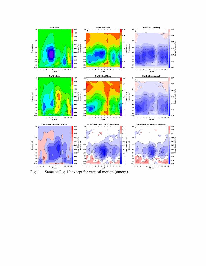
Fig. 11. Same as Fig. 10 except for vertical motion (omega).

Table 1. Resolutions of the various datasets used in this publication Dataset Temporal Areal Height ARM SGP MMCR 5 min < 60m (0.2° Beam) 90m GOES VISST ~15-30 min 0.5°x0.5° 3 levels NASA GISS SCM 1 hour 2.0°x2.5° 35 levels, ~25mb NARR Reanalysis 3 hour 0.3°x0.3° 29 levels, ~25mb ARM Cont. Forcing 1 hour 2.0°x2.5° 37 levels, ~25mb Table 2. Averaged cloud fraction (CF) and frequency of occurrence (Freq) from observations and model simulations during the period of 1999-2001.

Radar SAT(0.5o) SAT(2.5o) SCM(2.5o)

CF / Freq. CF / Freq. CF / Freq. CF / Freq. TOTAL 0.44 / 0.57 0.46 / 0.62 0.44 / 0.74 0.33-0.39 / 0.48

HIGH 0.30 / 0.42 0.21 / 0.36 0.19 / 0.46 0.15-0.18 / 0.19

MID 0.20 / 0.30 0.16 / 0.38 0.14 / 0.51 0.16-0.20 / 0.24

LOW 0.20 / 0.29 0.14 / 0.35 0.12 / 0.45 0.21-0.28 / 0.40

Table 3. Percentage of high cloud fraction occurring during stratiform conditions (omega ≥ 0) at the 500 mb level. Year DJF MAM JJA SON RAD Percentage 0.36 0.33 0.32 0.47 0.36 SCM Percentage 0.21 0.19 0.23 0.25 0.23

Table 4. Monthly linear Pearson correlation coefficients for observed and modeled cloud fractions with (a) relative humidity and (b) vertical pressure velocity. Values are given for both the ARM continuous forcing and NARR datasets. a. Relative Humidity 925mb 500mb 300mb CLDFR ARM NARR ARM NARR ARM NARR ARM TOTAL 0.65 0.73 0.7 0.72 0.84 0.89 ARM LOW 0.52 0.64 0.51 0.51 0.66 0.73 ARM MID 0.56 0.68 0.63 0.67 0.64 0.74 ARM HIGH 0.67 0.69 0.72 0.75 0.85 0.85 SCM TOTAL 0.84 0.57 0.57 SCM LOW 0.9 0.42 0.51 SCM MID 0.61 0.48 0.22 SCM HIGH 0.8 0.62 0.64 b. Omega 925mb 500mb 300mb CLDFR ARM NARR ARM NARR ARM NARR ARM TOTAL -0.01 0.02 -0.28 -0.48 -0.37 -0.69 ARM LOW -0.04 0.07 -0.18 -0.45 -0.3 -0.65 ARM MID 0.02 0.02 -0.21 -0.41 -0.3 -0.59 ARM HIGH -0.05 -0.03 -0.35 -0.42 -0.44 -0.62 SCM TOTAL -0.26 -0.6 -0.68 SCM LOW -0.25 -0.65 -0.73 SCM MID -0.27 -0.63 -0.63 SCM HIGH -0.32 -0.65 -0.75 Note that the strongest correlation in each row is given in bold. Values with a magnitude greater than 0.6 are considered to have a strong correlation, while those between 0.3-0.6 are moderate, and those less than 0.3 are weak.