Evaluation of the Information Content of Sedimentation Equilibrium Data in Self-Interacting Systems

Full Paper

798

Evaluation of the Information Contentof Sedimentation Equilibrium Data inSelf-Interacting Systems

Shirley Ang, Arthur J Rowe*

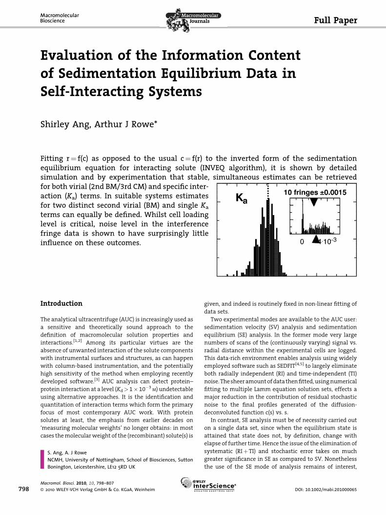
Fitting r¼ f(c) as opposed to the usual c¼ f(r) to the inverted form of the sedimentationequilibrium equation for interacting solute (INVEQ algorithm), it is shown by detailedsimulation and by experimentation that stable, simultaneous estimates can be retrievedfor both virial (2nd BM/3rd CM) and specific inter-action (Ka) terms. In suitable systems estimatesfor two distinct second virial (BM) and single Ka

terms can equally be defined. Whilst cell loadinglevel is critical, noise level in the interferencefringe data is shown to have surprisingly littleinfluence on these outcomes.

Introduction

The analytical ultracentrifuge (AUC) is increasingly used as

a sensitive and theoretically sound approach to the

definition of macromolecular solution properties and

interactions.[1,2] Among its particular virtues are the

absence of unwanted interaction of the solute components

with instrumental surfaces and structures, as can happen

with column-based instrumentation, and the potentially

high sensitivity of the method when employing recently

developed software.[3] AUC analysis can detect protein–

protein interaction at a level (Kd> 1� 10�3M) undetectable

using alternative approaches. It is the identification and

quantitation of interaction terms which form the primary

focus of most contemporary AUC work. With protein

solutes at least, the emphasis from earlier decades on

‘measuring molecular weights’ no longer obtains: in most

cases themolecularweight of the (recombinant) solute(s) is

S. Ang, A. J RoweNCMH, University of Nottingham, School of Biosciences, SuttonBonington, Leicestershire, LE12 5RD UK

Macromol. Biosci. 2010, 10, 798–807

� 2010 WILEY-VCH Verlag GmbH & Co. KGaA, Weinheim

given, and indeed is routinely fixed in non-linear fitting of

data sets.

Two experimental modes are available to the AUC user:

sedimentation velocity (SV) analysis and sedimentation

equilibrium (SE) analysis. In the former mode very large

numbers of scans of the (continuously varying) signal vs.

radial distance within the experimental cells are logged.

This data-rich environment enables analysis using widely

employed software such as SEDFIT[4,5] to largely eliminate

both radially independent (RI) and time-independent (TI)

noise.Thesheeramountofdata thenfitted,usingnumerical

fitting to multiple Lamm equation solution sets, effects a

major reduction in the contribution of residual stochastic

noise to the final profiles generated of the diffusion-

deconvoluted function c(s) vs. s.

In contrast, SE analysis must be of necessity carried out

on a single data set, since when the equilibrium state is

attained that state does not, by definition, change with

elapse of further time. Hence the issue of the elimination of

systematic (RIþ TI) and stochastic error takes on much

greater significance in SE as compared to SV. Nonetheless

the use of the SE mode of analysis remains of interest,

DOI: 10.1002/mabi.201000065

Evaluation of the Information Content of Sedimentation . . .

inasmuch as the time-invariance of the final state of the

system satisfies the requirements for true thermodynamic

analysis of that state, in which the ‘virial’ terms tradition-

ally used in the parameterization of the expansion with

respect to concentration of the chemical activity of the

solute(s) can be directly employed,[6] without a need for

consideration of ‘hydrodynamic non-ideality’ terms, as is

necessary in SV mode. An additional – but not necessarily

trivial – advantage of the SE mode is that both the total

experimental time takenand the amountof solutematerial

required for a seriesof experimentsareappreciably lower in

SE than in SV mode: especially since the use of multi-

channel cells enables three times more experiments to

be conducted in a given run in the formermode than in the

latter. To quantify this, let us briefly consider the resource

cost (i.e., 10mg�ml�1 solutematerial plus instrument time)

of estimatingasingleKavalue. For SVthedefinitionofans-c

isotherm over a set of seven concentrations (0.5–

10mg �ml�1, load volume 400 ml) would require � 13mg

in total over seven cells. Only 1Ka value can be evaluated

per run. In contrast, by SE, with only 80ml load volume, just

0.8mg is required, as a single SE experiments suffices to

establishvalues for the interaction term, the SEdistribution

itself sampling over a range of solute concentration. The

resource advantage of SE over SV become even more

markedwhenwe note that in a single SE run no fewer than

21Kavalues canbeevaluated (7� 3multi-sector cells). True,

an SE run takes longer than an SV run: but the difference in

resource requirement totally outweighs this factor.

However, the issue of the effects of error in the data sets

acquired in SE mode needs to be addressed, before we

confirm with confidence the above assertion, that ‘one

experiment suffices’. We find that in any attempt to fit SE

data, all of the following conditions need to be satisfied:

(i) t

Macro

� 20

he errors (systematic and stochastic) in the raw signal

values, and also in the radial values should have been

pre-determined for the instrument (the latter value is

trivial, it may be set at �0.5 pixel for Rayleigh

interference optics)

(ii) i
n every fit, the algorithm employed (Marquardt–
Levenberg or other) should incorporate the appro-

priate use of these provided error estimates in the

minimization (of the SSR or whatever) procedure

(iii) e
specially where the error surface is complex, the
Marquardt–Levenberg (ML) algorithm may not be

stable in use, even when initial parameter guesses

which are not unreasonable are provided.[7] Alter-

native algorithms need to be available for initial or

even final fitting, algorithms which may be slower

than ML but which can give stable initial estimates –

which should themselves be multiple[7] – for the

‘floated’ parameters. Our approach to obtaining a

stable fit involves three progressive steps: (i) use of

mol. Biosci. 2010, 10, 798–807

10 WILEY-VCH Verlag GmbH & Co. KGaA, Weinheim

real-time interactive manual fitting to obtain a good

approximation to optimal parameter values; (ii)

improvement of these estimates by re-fitting (without

statistical analysis but with input of data error

estimates) using a Robust algorithm; (iii) final re-

fitting using theML algorithmwith 500 iterations and

a confidence interval of 68.4%.

Wehavebeenable to satisfyall of theaboveconditionsby

performing our fits within the curve fitting and data

analysis packagepro Fit (QuantumSoft, Zurich) onanApple

Macintosh computer running under OS-X. This software is

capable, without user programming input, of meeting in a

user-friendly mode all of the requirements defined above.

Boot-strapping of parameter estimates and errors, for

example, is effected by simply entering in a dialog box

the estimated errors in the raw data, the number of iter-

ations required and the associated confidence interval (we

use the default of 68.4%). Completion of the fit then gen-

erates, in addition to the results, a full set of 500 estimates

for each floated parameter together with estimates for the

appropriate confidence intervals. Via a ‘Binning’ option

histogramsof theseparameterestimateare thengenerated.

As will be seen, the distribution of these estimates can be

very ‘non-Gaussian’ indeed.

Thevalueswhichweuse for our estimates of errors in the

raw data values are obtained experimentally, by a simple

subtractive procedure which eliminates – to a first

approximation – TI noise (RI noise is not relevant, since a

‘baseline offset’, which is in essence an RI noise value, is

floated in all our fits). Details of our approach, including our

handling of the issue of baseline distortion, are given below

(Experimental Part).

All our analyses are carried out using the INVEQ

functions, in which instead of fitting signal values as a

function of radial values, an inverse fit is performed, of

radial values as a function of signal value. The details are

given below. It needs to be emphasized that no ‘new

equation’ is being employed, merely a conventional

equation for SE, fitted after inversion as a means for

avoiding problems with the transcendental nature of the

equation as conventionally written. The INVEQ approach

hasbeenemployedsuccessfullybyourselvesandothers ina

range of applications.[6,8–12] In this present studywe define

more fully the extent to which a range of parameters can

be defined, showing that it is possible to retrieve sensible

values for interaction termsup to at least the 3rd virial term

in a single (but potentially self-interacting) solute system,

and we define the solute concentration values which are

called for. We find, perhaps surprisingly, that (all other

factors being equal) the level of the cell-loading concentra-

tion is considerably more crucial to success than is the

level of error in the raw signal data. We confirm via the

distribution of boot-strapped parameter estimates that our

www.mbs-journal.de 799

S. Ang, A. J. Rowe

800

earlier finding[6] concerning the complexnature of the error

surface in SE fitting is correct. Finally, we present

experimental data on a well-defined protein (RNAse A)

which show consistency with the results from our

simulations, and illustrate that results obtained by varying

the ionic strength of the solvent are consistent with

expectation in respect of the values of the interaction terms

yielded.

Experimental Part

Simulation

Simulated sedimentation equilibrium data were produced by

using the ‘Tabulate’ optionwithin pro Fit after appropriate values

for the selected parameters had been entered into the parameter

window, within the selected INVEQ function (inveq5aBC). Values

for the reference radius (rref) and for the reduced flotational

molecular weight (s) were fixed: other parameters, namely

reference solute concentration (cref), baseline offset (E), second

virial term(s) BMi, the third virial term CM, and the interaction

constant Ka were fixed for simulation, but floated for data

analysis. Note, the second and third virial ‘terms’ are the algebraic

product of the monomer molecular mass and the appropriate

‘virial coefficient’.

The simulations presented (selected from a more extensive set)

are for cell loading concentrations of ten fringe (�3mg �ml�1

protein) and 30 fringe (�10mg �ml�1 protein) with a reduced

floatational weight (see below) of s¼1.5, Ka¼0.0015 fringe�1,

BM¼0.0015ml � fringe�1 and CM¼ � 2e–6 fringe�2. These would

correspond to a Kd�14� 10�3M (at least one order of magnitude

weaker than a value measurable by other technologies), and

2BM�10 g �ml�1, not untypical for a globular proteinwith a small

net charge. The value for CM is at the lowest end of themagnitude

expected to be found for such a protein. It is not readily compared

with literature values, these being close to non-existent. All these

values are ‘conservative’, in the sense that they present a ‘case of

maximum difficulty’ for analysis. The reduced floatational weight

of s¼1.5 is again chosen partly in the interests of being

conservative. However there is also a practical reason for not

using larger values: at 30 fringe cell loading, no higher level is

feasible in ‘real life’ as thegradientsbecometoo steep tobe resolved

by the camera system of the Beckman XL-I. If one is performing

single runs at lower concentrations then of course the s value

(based upon rotor speed, see equation (2) below) can be increased,

with consequent gain in precision in parameter estimates. But

often inpractice onewill be runningmultiple samples together in a

rotorovera rangeof concentrations, and in this case the speedmust

be restricted to the speed appropriate to the highest concentration

used.

Data Analysis

The INVEQfunctions, as initiallydefined [8], fit thedatasetof (r,c) to

the followingequation,which is the simple algebraic inverse of the

conventionally defined equation for sedimentation equilibrium in

a system where a single second virial term BM defines the



expansion in c of the chemical potential at any radial position (r)

within the cell:

r ¼n�

ln cr=cið Þ þ 0:5� sw= 1þ 2BMcrð Þð Þ � r2i

�.�0:5� sw= 1þ 2BMcrð Þð Þ

�o0:5

(1)

where r is any radial position at which the solute concentration c

has the value cr, and ri and ci are the values of these parameters at

a defined reference position. The choice of this latter radial

position is not critical: it can sensibly be taken as being close to the

‘hinge point’ at which initial, cell-loading concentration is

conserved. The parameter s is the reduced molecular weight of

the solute, defined as

s ¼ M 1� vrð Þv2�RT (2)

where M is the molecular weight of the solute, v (ml � g�1) partial

specific volume, r the density of the solvent, v (radians/sec)

the angular velocity of the rotor, R the gas constant and T the

temperature (K). sw is the weight averaged value over the

monomer and the dimer, computed during every iteration during

the non-linear fitting of the parameters associated with

Equation (1) by solving from current value of Ka within the

iteration for a, the weight fraction of the total mass concentration

of the solute in dimer form at defined radial locus,

It must be stressed that Equation (1) is in no sense a ‘new’

equation. It is simply an inversion of the basic equation describing

the distribution at sedimentation equilibrium for the i’th solute

component as:

cr ¼ ca exp 0:5si 1þ @ ln g ið Þ=@crð Þcrf g r2a � r2� ��

(3)

where g i is the activity coefficient of that component. Clearly

for fitting purposes the activity term must be expressed in

terms of definite parameters, and a summation effected over all

species present. For present purposes we restrict ourselves to

two species (monomer and its dimer) being present, whose

weights are given via the law of mass action, characterized by

an equilibrium constant Ka. We follow conventional practice

and express the interaction in terms of the inverse of Ka, namely

Kd. In terms of a single second virial term, BM, (optionally)

assumed to be common to monomer and dimer, then

Equation (3) is written as

cr ¼ ca exp 0:5sw 1þ 2BMcrf g r2a � r2� ��

Z (4)

and the inversion of Equation (4) is seen to yield Equation (1).

There is however no limit in principle to the number of interaction

terms which could be written into Equation (3) prior to inversion.

The inner bracketed term can be written as

sw 1þ 2BMcr þ 3CMc2r�

(5)

for the case of values common to monomer and to dimer of

the second (2BM) and third (3CM) virial terms. Equally, for

two non-identical second virial terms, (BM)1 and (BM)2

DOI: 10.1002/mabi.201000065


characterizing the monomer and dimer, respectively, the inner

term is given as

Macrom

� 2010

s 1þ 2 a� 1ð Þ BMð Þ1cr þ 2a BMð Þ2cr�

(6)

where a represents the fraction of the total concentration of

monomers in dimer form, again derived directly from the Ka value

(which within the fit will be the current estimate of that

parameter).

It is important to understand however that there is a practical

limit to thenumberof interaction termswhich canbeadded, not in

terms of theory but in terms of the stability of the numerical

solutionswhichcanbeextracted. There isnopoint inaddinga large

numberof terms inanattempttoachieve ‘rigour’ if theoutcomeisa

set of equations incapable of simultaneous solution in terms of

numerical estimates obtainable for all these parameters.

In this latter context we must briefly address a recent doubt

whichhas been expressed[13]with regard to the INVEQapproach. It

is alleged that our derivation of the inverted equation (Equation 1)

requires the use of the Fujita-Adams[14] approximation; and also

attempts the algebraically impossible in defining both thermo-

dynamic and mass interaction parameters. Leaving aside the

(irrelevant) issue as towhether the assumption that (BM)1¼ (BM)2is or is not correctly attributed to ‘Fujita-Adams’, this assumption is

indeed onewhichwe havemade formany purposes: but it is in no

way required. No new equation is being ‘derived’, merely a re-

arrangementby trivial algebraofanexisting (universally accepted)

equation (Equation (3) above), with assignation of discrete

parameters to the thermodynamic interaction terms. As regards

the second allegation, we accept of course that in the limit of

infinite dilution the resolution of thermodynamic and interaction

termscannotbepossible, sinceonlya ‘limitingslope’, single-valued

of necessity, can be defined for the c-dependence: but we are not

restricting ourselves to this limiting state. Our present work

establishes further that not only is the INVEQ approach algebrai-

cally sound, but that the precision in experimental data is more

than sufficient for its practical implementation. Finally, as wewill

discuss further, we note that other workers using other methods

have successfully implemented an algorithm and practical

methods for the separate resolution of the thermodynamic and

mass interaction terms.[15] In particular, Zorrilla et al[15] – not

cited[13] – have described a ‘general model for self-association and

non-ideal repulsive interaction in a solution containing a single

solute component’ and formulated ‘an algorithm for simulta-

neously calculating the composition of solute species and signal

average buoyant molar mass of the solute as a function of its total

concentration’ (loci cit). A particular model (the long-established

‘hard sphere’ model) is used, and a long-duration, long-column

experimental system is employed, but the outcome is similar to

that given by the use of the (model free) INVEQ algorithm.

At this juncture, we note that there is an infinite set of

combinations of parameters which could be assigned when

we parameterize Equation (3). After second and third, why could

we not add fourth, fifth or higher virial terms? Why not assign

multiple Ka values for complex interactions? It has been our

intention in the work now presented to define just how many

stable parameter estimates it is possible to retrieve froma set of SE

data, at a level of precisionwhichyields results ‘of interest’. Initially

ol. Biosci. 2010, 10, 798–807

WILEY-VCH Verlag GmbH & Co. KGaA, Weinheim

and in our work published to date we have confined our enquiry –

subjectively – to the evaluation of lower (i.e., second) order

‘thermodynamic interaction parameters’, defined by conventional

virial terms, and by a single specific ‘weak’ (i.e., Kd� 0.1�10�3M)

interaction term. Thesehavebeen entered into the programcodeof

the function used as given in Equation (5) and (6).

Finally, the analysis of the data set, whether for simulated or for

real data, is routinely carried out within pro Fit (although the

precise software used is not critical, provided that the conditions

earlier defined aremet in the implementation). A single data point

in the region of the ‘hinge point’ of the equilibrium is selected, and

the co-ordinates (rref, cref) entered into the parameter window

associated with the function being employed. Estimates are

entered for the s value of the solute monomer derived via

SEDNTERP software for real solutes, for all the interaction terms

which are to be floated, and for a baseline offset E. Errors in initial

estimates for the latter quantity are generally large. But the INVEQ

functionshavebeencoded insuchawaythat cref is expectedtobe in

the form (signal þE) rather than signal, which causes the function

curve displayed in the Preview Window to rotate around the

selected central point as E is varied. Hence a surprisingly good

estimate for E can be obtained by simply ‘dragging’ this curvewith

E as the variable.

If this manual fit is clearly very close to the curve, then a ML fit

with 500 iterations using input error estimates for raw data is

performed, followed by binning and plotting out of histograms for

the parameter estimates. Otherwise, and in most cases, further

fitting in which the estimates for the interaction parameters are

refined is carried out, followed by the use of a Robust algorithm to

generate near-optimal parameter estimates prior toMLfitting. The

limits given for each parameter by the boot-strapping procedure at

the end of the MANUAL/Robust/ML fitting procedure are taken as

defining the quality of the estimate.

AUC Analysis

Highly purified salt-free lyophilized Bovine Pancreatic Ribonu-

clease A was purchased from Teknova (Hollister, California, USA).

After dissolving in PBS (phosphate buffered saline) adjusted to pH

7.0, or in this solvent pre-diluted to varying ionic strengths, the

concentration was checked spectrophotometrically and adjusted

by dilution to the required concentration. The nominal ionic

strengthof PBSwas taken for practical purposes to be 150�10�3M;

the exact value would vary slightly with pH. Simple proportional

dilution with water was performed to give a range of (again,

nominal) ionic strengths. A nominal ‘zero ionic strength’ solution

was achieved by dissolving the protein in water without pH

adjustment. Ultracentrifugal analysis was performed at 20 8C in a

Beckman XL-I Analytical Ultracentrifuge, using Rayleigh Inter-

ference Optics. A 2.5mm solution column length for both solution

and reference solventwas employed,withmeniscus level carefully

matched. Initial scans at 3 000 rpm.were recorded, to check for the

presence of any large aggregates. None were found. After

acceleration of the rotor to final speed (20 000 rpm) scans were

recorded immediately, and then every 2h until the patterns

recorded became time-invariant. Our instrument gives very level

fringepatterns for the ‘no redistribution’ case, andsuchvariation in

level along the course of the data region (TI noise) is small and not


S. Ang, A. J. Rowe

802

obviously reproducible from cell to cell. The use of a ‘blank’ cell is

thus pointless – a better removal of the TI noise is achieved by

subtracting the first scan at speed from the final selected scan, and

this we do. All scans were logged to disc using the Beckman

ProteomeLab software.

Results

Estimation of Error in Raw Data

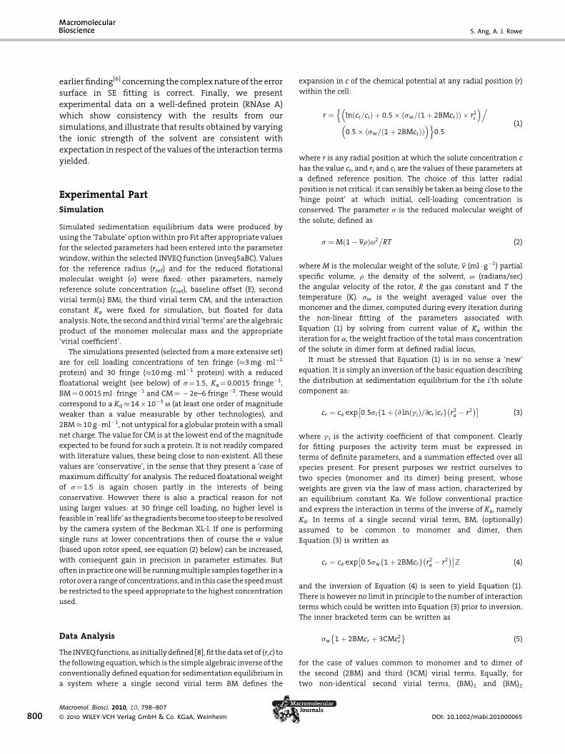
AsimpleExcel routine (FringeNoise.xls)hasbeenemployedto

attempt to eliminate TI noise and to give an estimate for the

stochasticnoise.Thetabulatedvaluesforthefringeincrement

over a range of 200 radial values are subtracted from the

values for the increment at the same radial values in the

preceding scan, and the tabulated differences thus produced

are plotted against radial value. This should eliminate TI

noise. Andwhere the average difference is clearly close to an

integral, then thealgebraic valueof that integral is subtracted

from the initial difference value, whichmostly eliminates RI

noise. Typical results are shown in Figure 1.

Clearlyhowever there is residual final (TI) noise present in

the distribution generated, over and above the (obvious)

stochastic noise. This residual noisewe termLow-Frequency

Anharmonicnoise (LFAnoise). It lacks repeating structure, as

investigated by Fourier analysis (not presented), and has an

Figure 1. Analysis of the error distribution in the Rayleigh interferenceof a sedimentation equilbrium scan from its predecessor scan (bothdeconvoluted into a low frequency noise component (2) and a high frthe distribution of the amplitudes in the latter yields an estimate (uppevery case refers to the index number, range 1–200, of consecutive



individualdistribution foreverypairofdata setsdifferenced.

Presumably some instrumental factor is involved, possibly

heat effects from the diffusion pump, or pixel instability in

the camera. We have achieved a deconvolution of the LFA

noise fromthe stochastic noise byuse of anO(12) orthogonal

polynomial fit (Figure 1). The stochastic noise is well

characterized, with a Gaussian distribution of values about

the mean, and a standard deviation from the mean of

�0.0015 fringe (1.5millifringe). This represents the ultimate

optimal performance of our instrument. The LFA noise is by

contrast clearly structured within its domain, and the

distribution about the mean cannot be truly Gaussian. We

have little choice however but to force a Gaussian fit onto

the values, and this yields an estimate of �0.0070 fringe

(7.0 millifringe) for the precision which obtains in actual

practice. The latter value we have used for the fitting of

practical data. We have however used both of these values

for simulationpurposes, in order tounderstand the extent to

which the elimination of this unwanted effect might

improve the precision of our parameter estimates.

Analysis of Simulated Data

Followingourearlierwork,wehave investigated theeffects

of solute loading concentration and of level of stochastic

optical system. The subtraction of 200 points from the central regionscans at equilibrium) results in a complex distribution (1) which is

equency stochastic noise component (1–2: bottom right). Analysis ofer, right) for the standard deviation of the central value. The x-axis indata points from the mid-region of the scan.

DOI: 10.1002/mabi.201000065


noise in the data on the precision of retrieval of input

parameters. Selected data from regions critical for valid

parameter retrieval are presented. Initiallywehave studied

the case of floating (Ka, BM) together with the baseline

offsetEandareferenceconcentrationvalue,uncorrected for

E, at a radial value located (butnot critically) in the regionof

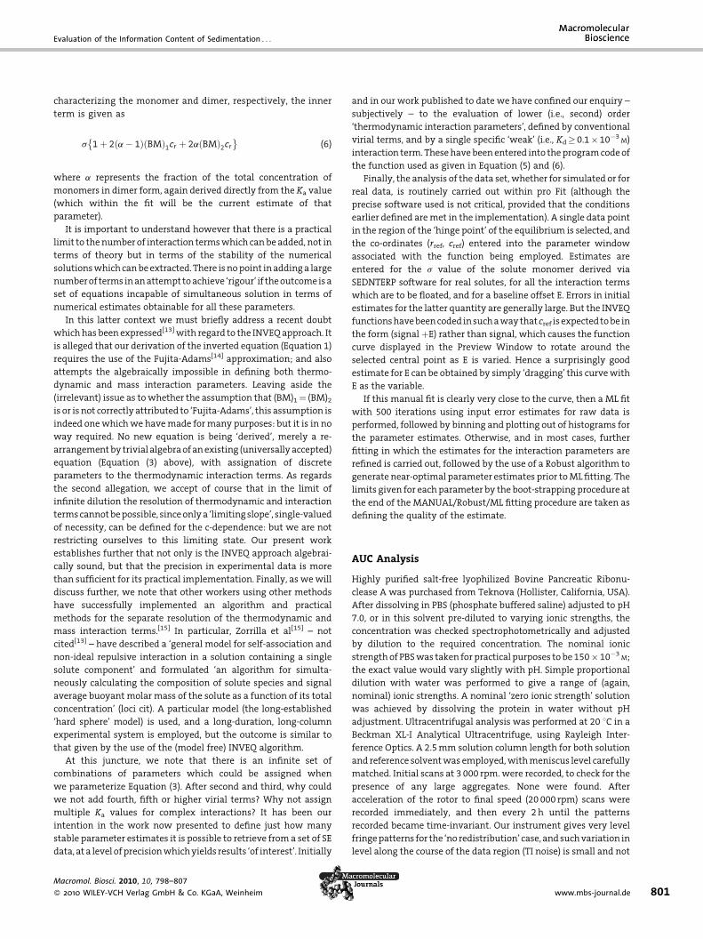
the ‘hingepoint’. Figure 2 (mainplots) shows the results of a

comparison of two cell loading concentrations (10 fringe or

30 fringe load) at two different levels of precision: namely

an ‘optimal’ data set with true stochastic noise only

(�0.0015 fringe) and a ‘realistic’ data set, in which the

LFA noise is present, and the overall distribution of the

total noise set is approximated by a gaussian distribution

(�0.0070 fringe). As is evident, very little difference

between the twoparameter sets is returned. Theparameter

distributions are all close to Gaussian, and on this basis a

standard deviation (SD) of the parameters Ka and BM

around the final estimate is calculated as � �1–3%. Thus

the level of error assumed to be present in the datamakes –

perhaps surprisingly– little ornodifference to theoutcome.

When the cell loading concentration is reduced to 3

fringe, however, the parameter distributions are very

Figure 2. Analysis for Ka and BM values in simulated data sets: s¼concentration¼ 10 fringe (main images) or 3 fringe (smaller inserted iParameter estimates are obtained from 500 iterations of the fit, errincrement) and �0.0002 (radial value) at 68.4% confidence interval. Vinserts, upward pointing arrows and downward pointing arrows indicaparameter estimates respectively



different (Figure 2, inset plots). Reflecting the known

complexity of the error surface for these fits, there is no

single peak present, but rather an approximately bi-modal

distribution, strongly skewed. The fit by ML is better than

might be expected, within �50% of input value, and the

weight-average of the parameters in the distribution is

even closer to input value (Figure 2, inset plots). However,

we are clearly on (or over) the borderline beyondwhich the

methodology is of practical use. Again, the level of error

added to the simulated data seems to have little relevance.

When an additional term (the third virial term, CM) is

added, then we would expect that higher cell loading

concentrations would need to be employed to obtain stable

fits. This is found to be the case. In Figures (main and inset

plots)we see the effect of theuse of concentrations of 30 and

10 fringe. At 30 fringe cell loading (main plots) it is clearly

possible to retrieve stable estimates for CM, SD� 5%, even at

the verynumerically low simulated value employed. For the

parameters Ka and BM the additional cell loading concen-

tration approximately compensates for the employment of

an additional parameter (CM) in the fit, and the precision

found for the parameters Ka and BM approximates to that

1.5; Ka¼BM¼0.0015 (fringe concentration units), with referencemages) and with normal random error added at the levels indicated.ors in the fitting routine fixed at �0.007 or þ0.0015 (for the fringeertical dashed lines indicate the input value of the parameter. On thete the estimates given by the LM fit and by the algebraic mean of the


S. Ang, A. J. Rowe

804

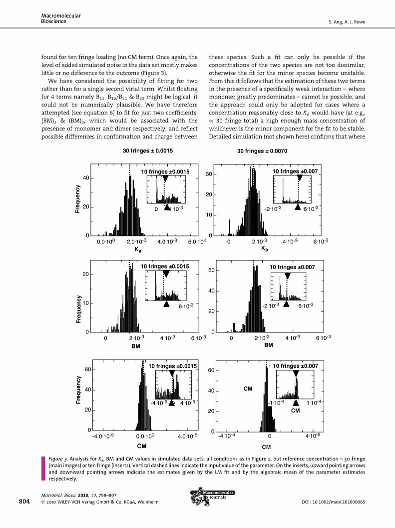
found for ten fringe loading (no CM term). Once again, the

level of added simulated noise in the data set mostly makes

little or no difference to the outcome (Figure 3).

We have considered the possibility of fitting for two

rather than for a single second virial term. Whilst floating

for 4 terms namely B11, B12/B21 & B22 might be logical, it

could not be numerically plausible. We have therefore

attempted (see equation 6) to fit for just two coefficients,

(BM)1 & (BM)2, which would be associated with the

presence of monomer and dimer respectively, and reflect

possible differences in conformation and charge between

Figure 3. Analysis for Ka, BM and CM values in simulated data sets: a(main images) or ten fringe (inserts). Vertical dashed lines indicate theand downward pointing arrows indicate the estimates given by threspectively.



these species. Such a fit can only be possible if the

concentrations of the two species are not too dissimilar,

otherwise the fit for the minor species become unstable.

From this it follows that the estimation of these two terms

in the presence of a specifically weak interaction – where

monomer greatly predominates – cannot be possible, and

the approach could only be adopted for cases where a

concentration reasonably close to Kd would have (at e.g.,

� 30 fringe total) a high enough mass concentration of

whichever is the minor component for the fit to be stable.

Detailed simulation (not shown here) confirms that where

ll conditions as in Figure 2, but reference concentration¼ 30 fringeinput value of the parameter. On the inserts, upward pointing arrowse LM fit and by the algebraic mean of the parameter estimates

DOI: 10.1002/mabi.201000065


these conditions can be met, then two second virial terms

can be defined: but few real-life systems will meet these

conditions. The resolution of two second virial terms must

thus be regarded as algebraically possible, but algorithmi-

cally impracticable in most cases.

Analysis of Experimental Data

We have examined sedimentation equilibrium data for a

range of concentrations of RNAse A. To demonstrate the

precision and power of the methodology, as applied to real

data, we have examined the way in which the parameter

set (Ka, BM, CM) is affected by variation in ionic strength.

Low or very low ionic strength should, in terms of simple

theory, lead to an expansion of the electrical double layer,

causing the inter-molecular repulsion to increase, and

henceKa to decrease, whilst charge effects would cause BM

to increase and a significant CM term to appear.

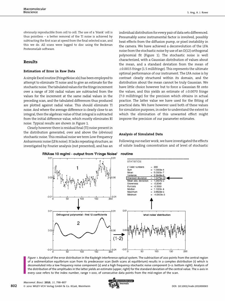
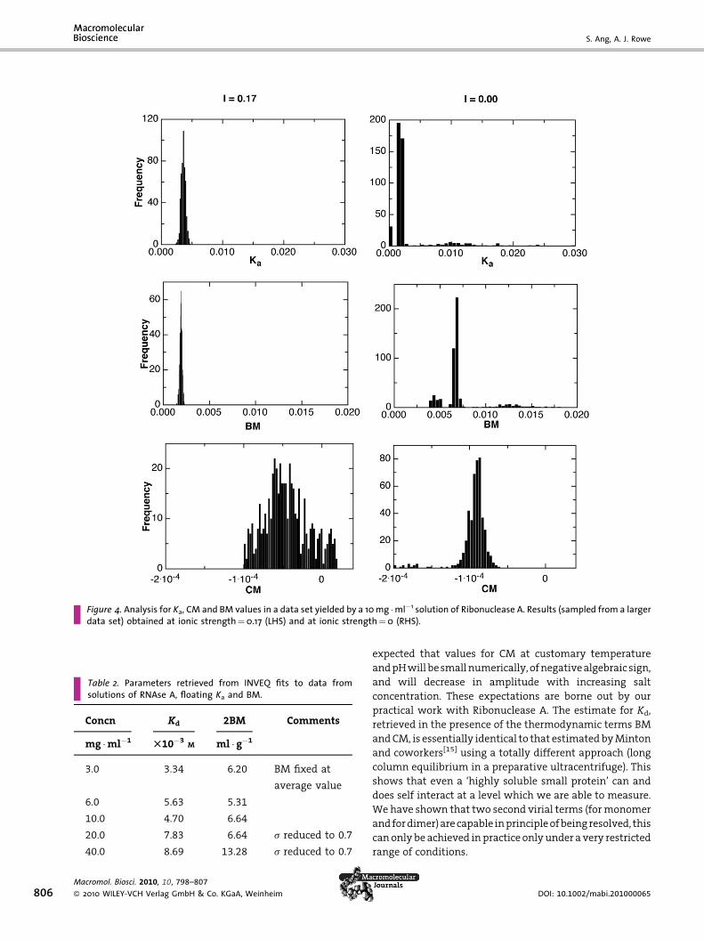
The results which we obtain are given in Table 1, and

illustrated in Figure 4. We note that the parameter

distributions are in some cases a little less unimodal than

in the simulations, but overall, expectations are borne out.

The precision with which quality estimates for CM can be

retrievedunder conditionswhere itwill besmall invalue isa

little less good than simulation might suggest, and the

spreadof theCMparameterestimatesunder suchconditions

(Figure 4) is rather wide. The possibility that fourth virial

term(s) couldbepresentmightbea factorhere.Butexactlyas

predicted, we see that an expansion of the electrical double

layer causes results inadecrease inKa, an increase inBMand

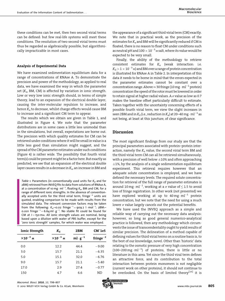
Table 1. Parameters (in conventionally used units for Kd and for2BM) retrieved from INVEQ fits to data from solutions of RNAse A,at a concentration of 10 mg �ml�1, floating Ka, BM and CM, for arange of different ionic strengths. In the absence of convention-ally accepted units for the third virial term, fringe�2 units arequoted, enabling comparison to be made with results from thesimulated data. The relevant conversion factors may be takenfrom the following: Ka:–0.02 fringe�1¼909.7 l �mol�1; 2BM:–0.001 fringe�1¼6.64 ml �g�1. No stable fit could be found forCM at I¼ 150 mM. All ionic strength values are nominal, beingbased upon a dilution with water of PBS buffer, except for the‘zero ionic strength’ samples, for which water was employed.

Ionic Strength Kd 2BM CM�1e5

T10�3M T10�3

M ml � g�1 fringe�2

0.0 12.2 44.4 �9.00

3.0 15.7 21.1 �6.35

5.0 15.1 32.0 �6.76

9.0 15.7 21.1 �5.40

17.0 2.9 27.4 �0.77

150 4.7 6.6 ND



theappearanceof a significant thirdvirial term (CM)exactly.

We note that in practical work, as the precision of the

estimates forKa andBMwill be significantly reduced if CMis

floated, there is no reason to float CMunder conditions such

asneutralpHand100� 10�3Msalt,where itsvaluewouldbe

expected to be very small.

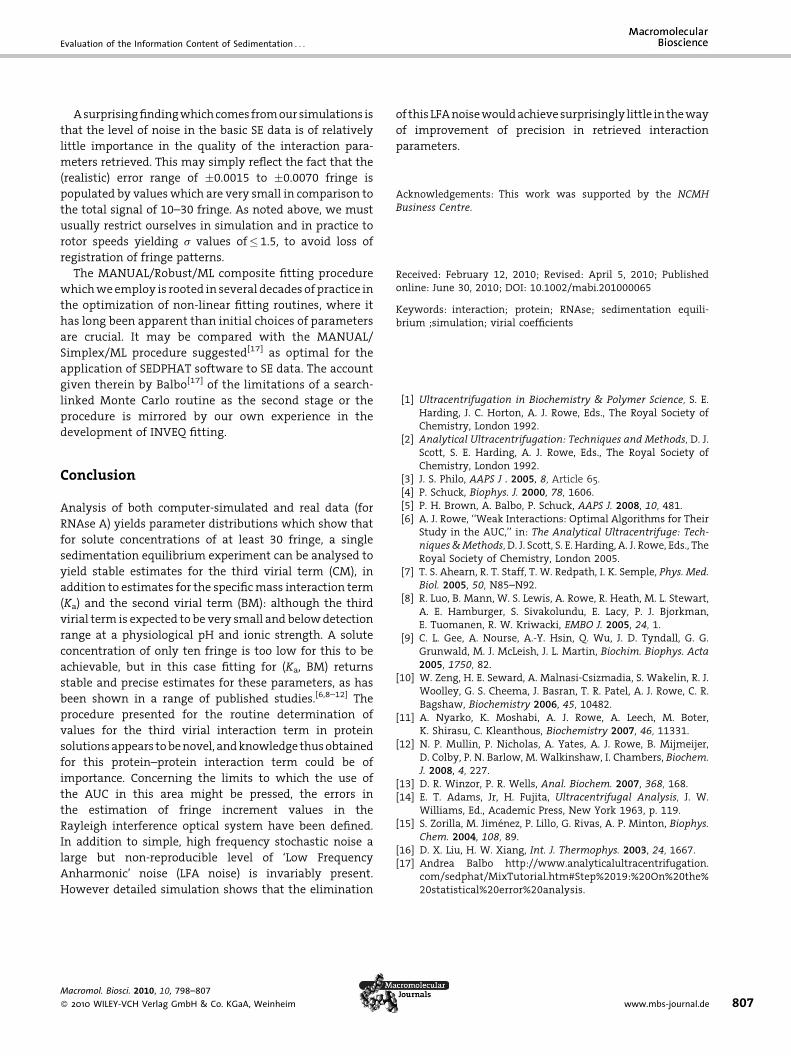
Finally, the ability of the methodology to retrieve

consistent estimates for Ka (weak interaction: i.e.

Kd> 1� 10�3M)andBMoverarangeofproteinconcentration

is illustrated for RNAse A in Table 2. In interpretation of this

data it needs to be borne inmind that the errors expected in

the parameter estimates cannot be constant over a

concentrationrange.Above�30fringe (10mg �ml�1protein)

concentration the speedof the rotormustbe lowered inorder

to retain signal at higher radial values. A s value as lowas 0.7

makes the baseline offset particularly difficult to estimate.

Taken together with the uncertainty concerning effects of a

possible fourth virial term, we view the slight increases in

seen2BMand inKd (i.e., reduction inKa) at20–40mg �ml�1as

not being, at least at this juncture, of clear significance.

Discussion

The most significant findings from our study are that the

principal parameters associatedwith protein–protein inter-

action, namely the Ka value, the second virial term BM and

the third virial termCM can all be retrieved simultaneously,

with a precision ofwell below�10% and often approaching

�1%, by the analysis of a single sedimentation equilibrium

experiment. This retrieval requires however that an

adequate solute concentration is employed, and we have

defined the necessary levels. The required solute concentra-

tion for retrieval of the full range of parameter estimates is

around 10mg �ml�1, working at a s value of� 1.5 to avoid

loss of fringe registration. In other work (not presented) we

have explored working at up to 40mg �ml�1 protein

concentration, but we note that the need for using a much

lower s value largely cancels out the potential benefits.

We have used the INVEQ approach as a simple and

reliable way of carrying out the necessary data analysis:

however, so long as good general numerico-analytical

practice is followed, then any methodology which circum-

vents the issueof transcendentality ought toyield results of

similar precision. The delineation of a method capable of

defining values for third virial terms on a routine basis is, to

the best of our knowledge, novel. Other than ‘historic’ data

relating to the osmotic pressure of very high concentration

(100–200mg �ml�1) of proteins, there is little or no

literature in this area. Yet since the third viral term defines

an attractive force, and its contribution to the total

interaction between protein monomers is not negligible

(current work on other proteins), it should not continue to

be overlooked. On the basis of limited theory[16] it is


S. Ang, A. J. Rowe

Figure 4. Analysis for Ka, CM and BM values in a data set yielded by a 10 mg �ml�1 solution of Ribonuclease A. Results (sampled from a largerdata set) obtained at ionic strength¼0.17 (LHS) and at ionic strength¼0 (RHS).

Table 2. Parameters retrieved from INVEQ fits to data fromsolutions of RNAse A, floating Ka and BM.

Concn Kd 2BM Comments

mg �ml�1 T10�3M ml � g�1

3.0 3.34 6.20 BM fixed at

average value

6.0 5.63 5.31

10.0 4.70 6.64

20.0 7.83 6.64 s reduced to 0.7

40.0 8.69 13.28 s reduced to 0.7

806Macromol. Biosci. 2010, 10, 798–807


expected that values for CM at customary temperature

andpHwillbesmallnumerically, ofnegativealgebraic sign,

and will decrease in amplitude with increasing salt

concentration. These expectations are borne out by our

practical work with Ribonuclease A. The estimate for Kd,

retrieved in the presence of the thermodynamic terms BM

andCM, is essentially identical to that estimatedbyMinton

and coworkers[15] using a totally different approach (long

column equilibrium in a preparative ultracentrifuge). This

shows that even a ‘highly soluble small protein’ can and

does self interact at a level which we are able to measure.

We have shown that two second virial terms (formonomer

andfordimer)arecapable inprincipleofbeingresolved, this

canonlybe achieved inpractice onlyunder a very restricted

range of conditions.

DOI: 10.1002/mabi.201000065


Asurprisingfindingwhichcomes fromoursimulations is

that the level of noise in the basic SE data is of relatively

little importance in the quality of the interaction para-

meters retrieved. This may simply reflect the fact that the

(realistic) error range of �0.0015 to �0.0070 fringe is

populated by valueswhich are very small in comparison to

the total signal of 10–30 fringe. As noted above, we must

usually restrict ourselves in simulation and in practice to

rotor speeds yielding s values of� 1.5, to avoid loss of

registration of fringe patterns.

The MANUAL/Robust/ML composite fitting procedure

whichweemploy is rooted in several decades of practice in

the optimization of non-linear fitting routines, where it

has long been apparent than initial choices of parameters

are crucial. It may be compared with the MANUAL/

Simplex/ML procedure suggested[17] as optimal for the

application of SEDPHAT software to SE data. The account

given therein by Balbo[17] of the limitations of a search-

linked Monte Carlo routine as the second stage or the

procedure is mirrored by our own experience in the

development of INVEQ fitting.

Conclusion

Analysis of both computer-simulated and real data (for

RNAse A) yields parameter distributions which show that

for solute concentrations of at least 30 fringe, a single

sedimentation equilibrium experiment can be analysed to

yield stable estimates for the third virial term (CM), in

addition to estimates for the specificmass interaction term

(Ka) and the second virial term (BM): although the third

virial term is expected to be very small and belowdetection

range at a physiological pH and ionic strength. A solute

concentration of only ten fringe is too low for this to be

achievable, but in this case fitting for (Ka, BM) returns

stable and precise estimates for these parameters, as has

been shown in a range of published studies.[6,8–12] The

procedure presented for the routine determination of

values for the third virial interaction term in protein

solutionsappears tobenovel, andknowledge thusobtained

for this protein–protein interaction term could be of

importance. Concerning the limits to which the use of

the AUC in this area might be pressed, the errors in

the estimation of fringe increment values in the

Rayleigh interference optical system have been defined.

In addition to simple, high frequency stochastic noise a

large but non-reproducible level of ‘Low Frequency

Anharmonic’ noise (LFA noise) is invariably present.

However detailed simulation shows that the elimination



of this LFAnoisewouldachievesurprisingly little in theway

of improvement of precision in retrieved interaction

parameters.

Acknowledgements: This work was supported by the NCMHBusiness Centre.

Received: February 12, 2010; Revised: April 5, 2010; Publishedonline: June 30, 2010; DOI: 10.1002/mabi.201000065

Keywords: interaction; protein; RNAse; sedimentation equili-brium ;simulation; virial coefficients

[1] Ultracentrifugation in Biochemistry & Polymer Science, S. E.Harding, J. C. Horton, A. J. Rowe, Eds., The Royal Society ofChemistry, London 1992.

[2] Analytical Ultracentrifugation: Techniques and Methods, D. J.Scott, S. E. Harding, A. J. Rowe, Eds., The Royal Society ofChemistry, London 1992.

[3] J. S. Philo, AAPS J . 2005, 8, Article 65.[4] P. Schuck, Biophys. J. 2000, 78, 1606.[5] P. H. Brown, A. Balbo, P. Schuck, AAPS J. 2008, 10, 481.[6] A. J. Rowe, ‘‘Weak Interactions: Optimal Algorithms for Their

Study in the AUC,’’ in: The Analytical Ultracentrifuge: Tech-niques&Methods,D. J. Scott, S. E. Harding, A. J. Rowe, Eds., TheRoyal Society of Chemistry, London 2005.

[7] T. S. Ahearn, R. T. Staff, T. W. Redpath, I. K. Semple, Phys. Med.Biol. 2005, 50, N85–N92.

[8] R. Luo, B. Mann, W. S. Lewis, A. Rowe, R. Heath, M. L. Stewart,A. E. Hamburger, S. Sivakolundu, E. Lacy, P. J. Bjorkman,E. Tuomanen, R. W. Kriwacki, EMBO J. 2005, 24, 1.

[9] C. L. Gee, A. Nourse, A.-Y. Hsin, Q. Wu, J. D. Tyndall, G. G.Grunwald, M. J. McLeish, J. L. Martin, Biochim. Biophys. Acta2005, 1750, 82.

[10] W. Zeng, H. E. Seward, A. Malnasi-Csizmadia, S. Wakelin, R. J.Woolley, G. S. Cheema, J. Basran, T. R. Patel, A. J. Rowe, C. R.Bagshaw, Biochemistry 2006, 45, 10482.

[11] A. Nyarko, K. Moshabi, A. J. Rowe, A. Leech, M. Boter,K. Shirasu, C. Kleanthous, Biochemistry 2007, 46, 11331.

[12] N. P. Mullin, P. Nicholas, A. Yates, A. J. Rowe, B. Mijmeijer,D. Colby, P. N. Barlow, M. Walkinshaw, I. Chambers, Biochem.J. 2008, 4, 227.

[13] D. R. Winzor, P. R. Wells, Anal. Biochem. 2007, 368, 168.[14] E. T. Adams, Jr, H. Fujita, Ultracentrifugal Analysis, J. W.

Williams, Ed., Academic Press, New York 1963, p. 119.[15] S. Zorilla, M. Jimenez, P. Lillo, G. Rivas, A. P. Minton, Biophys.

Chem. 2004, 108, 89.[16] D. X. Liu, H. W. Xiang, Int. J. Thermophys. 2003, 24, 1667.[17] Andrea Balbo http://www.analyticalultracentrifugation.

com/sedphat/MixTutorial.htm#Step%2019:%20On%20the%20statistical%20error%20analysis.


Evaluation of the Information Content of Sedimentation Equilibrium Data in Self-Interacting Systems

Documents

Transcript of Evaluation of the Information Content of Sedimentation Equilibrium Data in Self-Interacting Systems