EVALUATION OF THE DETECTION AND … · iii LIST OF FIGURES Figure 1. ... CSD Cutter Suction Dredger...
72
EVALUATION OF THE DETECTION AND QUANTIFICATION OF SEDIMENT PLUMES CAUSED BY DREDGING ACTIVITIES USING A MULTIBEAM ECHOSOUNDER Nils Lowie Student number: 01200387 Promotor: Prof. dr. David Van Rooij Copromotor: Koen Degrendele Jury: Prof. dr. Marc De Batist, dr. Michael Fettweis Master’s dissertation submitted in partial fulfilment of the requirements for the degree of Master of Science in Geology Academic year: 2016 – 2017
Transcript of EVALUATION OF THE DETECTION AND … · iii LIST OF FIGURES Figure 1. ... CSD Cutter Suction Dredger...

EVALUATION OF THE DETECTION AND
QUANTIFICATION OF SEDIMENT
PLUMES CAUSED BY DREDGING
ACTIVITIES USING A MULTIBEAM
ECHOSOUNDER
Nils Lowie Student number: 01200387
Promotor: Prof. dr. David Van Rooij
Copromotor: Koen Degrendele
Jury: Prof. dr. Marc De Batist, dr. Michael Fettweis
Master’s dissertation submitted in partial fulfilment of the requirements for
the degree of Master of Science in Geology
Academic year: 2016 – 2017


i
ACKNOWLEDGEMENTS
Writing a master thesis is a work to which a lot of people contributed in a direct or indirect way. It is
also the crown on my education of five years. It would therefore like to use this page to thank everyone
who helped and supported me in this journey, including you, the reader, for taking interest in this.
Several times throughout the process of writing this work and more in general my study I could make
the comparison with a multibeam survey. Therefore I’ll tell this story in analogy to a survey vessel.
Firstly I have to thank the captains who guided the vessel through the weather. I would like to thank
my promotors who helped me getting this thesis written in particular. Thank you prof. Van Rooij for
the reads of the drafts, constructive comments and trusting me into doing my own thing in a relatively
unsearched field under the good guidance of my co-promotors. One of the most important guys I have
to thank for this work, probably the head-captain of this ship, is my co-promoter Koen Degrendele.
Thank you for the discussions on this topic and other, for letting me write at my own (slow) pace, and
thank you for the reading and corrections. Together with Marc you gave me every possible chance (I
refer to the ‘Story of My Research’ part for this). I learned a lot from all the presentations in which you
guided me and it helped me to be more confident in presenting. It even helped me to get the dream
job I wanted at one of my dream companies, and therefore I am forever grateful to the both of you.
A vessel is nothing without its crewmembers to operate everything and keep things going. I would like
to thank prof. Bertrand, Elke and Loic for guiding me into the world of grain size analysis and thank
them for their time explaining everything related to it. Thank you to the crew of RV Simon Stevin and
thank you to my colleagues at the CSS for their pleasant company at noon when eating.
A vessel cannot navigate without fuel, which I consider as both emotional as financial support. For the
latter I would like to thank the FPS Economy for paying my trip to Rennes and travel expenses. Lastly
as for emotional support I would like to thank the following people.
Lies(beth), although our ways have parted now, I thank you for the first four years of my study in which
you were my biggest support. Not mentioning you here would be unfair to the truth and I will not
forget the big part of you in this story.
Thank you to my friends, for all the (un)forgettable nights out and the stud(ie)ing together. Thank you
to my classmates and Geologica friends for the nice moments and excursions. Thank you to some best
friends in particular: Simon, Dolf, Ricardo, Mathias, Rob and Stan, especially for your special support
during the beginning and first semester of this last studying year. Thank you Eline for your recent
support!
Merci oma en pepe en de rest van mijn familie voor de steunende berichtjes voor een examen. Lars,
Amber en Jinte, merci om mijn soms rare stressdansjes te verdragen, mijn plagende opmerkingen en
meer gedurende examenperiodes en periodes van stress (dat wil niet zeggen dat jullie er nu van af
zijn!).
Mama en papa. Deze campagne was een campagne met veel storm en mooi weer afgewisseld. Weer
is altijd de onzekere factor, maar er was doorheen mijn studie één zekerheid: jullie waren de sterke
mast van het schip die alles overeind hield, ervoor zorgde dat het schip niet zonk, het onderdeel van
het geheel waar ik altijd kon op rekenen. Bedankt om doorheen woelige periodes met veel stress en
mijn niet altijd vriendelijk zijn toch achter mij te blijven staan en mij onvoorwaardelijk te steunen.
Merci om mij de kans te geven om te studeren en dus de financiële support. Ik kon mij geen betere
ouders/houvast voorstellen.

ii

iii
LIST OF FIGURES
Figure 1. The Belgian Continental Shelf with the sandbanks and the sectors of monitoring on it
(Degrendele et al., 2014). ......................................................................................................................... 2
Figure 2. Extracted volume per month, cumulative volume and mean depth difference with reference
model of S1a (2001-2004) calculated along a profile in monitoring zone TBMAB (Roche et al., 2017). . 2
Figure 3. Illustration of the overspill from the barge and the dragging of the suction head, which will
lead to a dynamic sediment plume and a passive sediment plume (Spearman et al., 2011).................. 4
Figure 4. Location and bathymetry of the North Sea situated northwest of Europe. ............................ 5
Figure 5. Semidiurnal tides M2 and S2 in the North Sea (Pohlmann and Sündermann, 2011). ............. 6
Figure 6. The Belgian Continental Shelf with its sandbanks. Mathys (2009) modified from Le Bot et al.
(2003).. ..................................................................................................................................................... 7
Figure 7. Patch line test to determine the time delay. Figure from Mann (1998) modified after (Godin,
1996). ..................................................................................................................................................... 13
Figure 8. Patch line test to determine the pitch bias. Figure from (Mann, 1998) modified after (Godin,
1996). ..................................................................................................................................................... 13
Figure 9. Calculation of the yaw bias. Figure by courtesy of L3 Communications ELAC Nautik. ........... 14
Figure 10. Screenshot from FMMidwater. Fan view of the water column. ........................................... 20
Figure 11. Screenshot from FMMidwater. Stacked view of the water column.. ................................... 20
Figure 12. Screenshot of the water column backscatter histogram. ..................................................... 20
Figure 13. The echo-integration principle. (Figure by courtesy of IFREMER). ....................................... 21
Figure 14. Workflow chart of the processing in Voxler. ........................................................................ 23
Figure 15. The coordinate transformation program written by the CSS ............................................... 25
Figure 16. The backscatter extraction program written by the CSS. ..................................................... 26
Figure 17. The vessel track comparison program written by the CSS. .................................................. 26
Figure 18. Bathymetry of a part of the Thorntonbank which shows the general outline of this particular
area with an outlet in which later-on the TSHD will pass. ..................................................................... 27
Figure 19. Bathymetry of the track following the Ruyter (TBMAB16-730)............................................ 28
Figure 20. Shaded relief grid of the track following the Ruyter (TBMAB16-730) .................................. 28
Figure 21. Difference grid of the Ruyter track (1m resolution) ............................................................. 29
Figure 22. Bathymetry of the Thorntonbank two months after the studied dredging took place. ....... 29
Figure 23. Backscatter mosaic of a part of the Thorntonbank which shows the uniform backscatter. 30
Figure 24. Backscatter grid of the Ruyter track (TBMAB16-730) made using FMGT. ............................ 31
Figure 25. Backscatter grid of the Ruyter track (TBMAB16-730) made using Sonarscope. ................... 31
Figure 26. Intensity of the sediment plume resulting from the SonarScope echo-integration algorithm.
................................................................................................................................................................ 33

iv
Figure 27. Raw backscatter values from a part of the sediment plume caused by TSHD the Ruyter.. . 34
Figure 28. Volume render of the sediment plume caused by TSHD the Ruyter .................................... 35
Figure 29. Face render of the sediment plume caused by TSHD the Ruyter ......................................... 35
Figure 30. Plume intensity in function of the distance between TSHD the Ruyter and RV Simon
Stevin. ..................................................................................................................................................... 36
Figure 31. Plume intensity in function of the distance between TSHD the Ruyter and RV Simon
Stevin. ..................................................................................................................................................... 36
Figure 32. Comparison between the in-situ grain size data and the grain size data from the dredged
material itself. ........................................................................................................................................ 38
Figure 33. Plot of the navigation data on the shaded relief map following TSHD Ruyter ..................... 39
Figure 34. Plume intensity along TSHD Ruyter track. The vectors show the current direction. ........... 41
Figure 35. Intensity of the sediment plume resulting from the SonarScope echo-integration algorithm
not taking the outer 35 degrees into account of the water column on both sides ............................... 42
Figure 36. Stacked view of line 32 of the Ruyter track. ......................................................................... 43
Figure 37. Sideway look on the resulting face render model for line 32 of the Ruyter track. ............... 43
Figure 38. Echogram of water column with a good range set to filter out side lobe interference. ...... 44
Figure 39. The accompanying stacked view of figure 38. ...................................................................... 45

v
LIST OF TABLES
Table 1. Location offsets on RV Simon Stevin. ....................................................................................... 12
Table 2. Offset angles (degrees) for the calibration of the EM2040 echosounder of RV Simon Stevin.15
Table 3. Location, date and remarks of the 9 samples acquired during survey TBMAB16-310.. .......... 17
Table 4. Location, date and remarks of the 3 samples acquired during survey TBMAB16-730. ........... 17
Table 5. Overview of the bathymetric results for all the tracks. ........................................................... 30
Table 6. Overview of the seafloor backscatter results for all the tracks in FMGT. ................................ 32
Table 7. Overview of the seafloor backscatter results for all the tracks in SonarScope. ...................... 32
Table 8. Overview of the correlation coefficient results for all tracks. .................................................. 37
Table 9. Grain size results of the fraction less than 1 mm from the samples on the Thorntonbank. ... 37
Table 10. Grain size results of the three taken samples after dredging along the track of the TSHD
Interballast. Only the fraction smaller than 1mm was analysed. .......................................................... 38
Table 11. Grain size results of a total of 46 samples taken from the dredged material that is used in
building applications. ............................................................................................................................. 38

vi
LIST OF ABBREVIATIONS
ADCP Acoustic Doppler Current Profiler
BCS Belgian Continental Shelf
BD Backhoe Dredger
BPNS Belgian Part of the North Sea
CSD Cutter Suction Dredger
CTD Conductivity, Temperature and Depth
CUBE Combined Uncertainty and Bathymetry Estimator
dB Decibel
EEZ Exclusive Economic Zone
FMGT FlederMaus Geocoder Toolbox
IFREMER Institut Français de Recherche pour l’Exploitation de la Mer
MBES Multibeam Echosounding System
PSU Practical Salinity Unit
RTK Real Time Kinematic
RV Research Vessel
SBS Seafloor Backscatter
SPI Sediment Profile Images
SPM Suspended Particulate Matter
SVP Sound Velocity Probe
TSHD Trailing Suction Hopper Dredger
WCBS Water Column Backscatter

vii
TABLE OF CONTENTS
CHAPTER I INTRODUCTION ..................................................................................................... 1
1.1. Sand extraction on the Belgian Continental Shelf ...................................................................... 1
1.2. Objectives ................................................................................................................................... 3
CHAPTER II GEOLOGICAL SETTING ............................................................................................ 5
2.1. The North Sea ............................................................................................................................. 5
2.2. The Belgian part of the North Sea .............................................................................................. 7
2.3. The Thorntonbank ...................................................................................................................... 8
CHAPTER III MATERIAL AND METHODS ..................................................................................... 9
3.1. Dredging ...................................................................................................................................... 9
3.1.1. Different kind of dredging vessels ...................................................................................... 9
3.1.2. Dredging vessels followed in this work ............................................................................. 10
3.1.3. Electronic Monitoring Systems ......................................................................................... 10
3.2. Surveying ................................................................................................................................... 11
3.2.1. Principle and calibration of MBES ..................................................................................... 11
3.2.2. Bathymetry and Seafloor backscatter .............................................................................. 15
3.2.3. Water column backscatter ................................................................................................ 15
3.2.4. Sampling ............................................................................................................................ 16
3.3. Processing of acoustic data ....................................................................................................... 18
3.3.1. Processing in Qimera ........................................................................................................ 18
3.3.2. Processing in FMGeocoder Toolbox (FMGT) .................................................................... 19
3.3.3. Processing in FMMidwater ............................................................................................... 19
3.3.4. Processing in SonarScope ................................................................................................. 21
3.3.5. Processing in Surfer 12...................................................................................................... 22
3.3.6. Processing in Voxler .......................................................................................................... 22
3.4. Processing of the sand samples ................................................................................................ 23
3.5. Processing of navigation files and EMS..................................................................................... 24
3.5.1. Influence of distance on the detection of sediment plumes ............................................ 25
3.5.2. Influence of time since passing on the detection of sediment plumes ............................ 26

viii
CHAPTER IV RESULTS .............................................................................................................. 27
4.1. Bathymetry ............................................................................................................................... 27
4.1.1. Bathymetry right before dredging .................................................................................... 27
4.1.2. Bathymetry directly after dredging .................................................................................. 27
4.1.3. Bathymetry two months after dredging ........................................................................... 29
4.1.4. Overview all tracks ............................................................................................................ 30
4.2. Seafloor backscatter ................................................................................................................. 30
4.2.1. Seafloor backscatter right before and two months after dredging .................................. 30
4.2.2. Seafloor backscatter directly after dredging .................................................................... 31
4.2.3. Overview of all tracks ........................................................................................................ 32
4.3. Water column backscatter ........................................................................................................ 33
4.3.1. Two-dimensional results ................................................................................................... 33
4.3.2. Three-dimensional results ................................................................................................ 34
4.4. Influence of time or distance between vessels on the plume intensity ................................... 36
4.4.1. Results for TSHD Ruyter .................................................................................................... 36
4.4.2. Overview results for the other tracks ............................................................................... 37
4.5. Grain size analysis ..................................................................................................................... 37
CHAPTER V DISCUSSION ........................................................................................................ 39
5.1. Evolution of the tracks on bathymetry ..................................................................................... 39
5.2. Impact and evolution on seafloor with SBS .............................................................................. 40
5.3. Visualization of the sediment plumes....................................................................................... 41
5.3.1. Quality of the visualizations in two and three dimensions............................................... 41
5.3.2. The difficulty of processing water column data with sediment plumes........................... 44
5.4. Possible grain size of the sediment plume ............................................................................... 45
5.5. Impact of measurement conditions on results ......................................................................... 45
CHAPTER VI CONCLUSION ....................................................................................................... 47
REFERENCES ........................................................................................................................... 49
APPENDIX ........................................................................................................................... 55

ix
THE STORY OF MY RESEARCH
The story of my research can be told from the initial beginning, which probably even dates back to
when I was 13 to 14 years old. As a young student in secondary school I was always fascinated by
nature, watching a lot of documentaries on television, always interested in how things worked. I
studied Latin in my first four years of middle school, followed by a transition to the science-
mathematics direction in my last two years. I was very interested in the whole of sciences with mainly
physics and geography as highest interests. This preference for sciences made me after a long
consideration choose for trying to obtain a bachelor’s degree in geology at Ghent University because
of its combining of biology, chemistry, physics, geography, geology and a bit of mathematics.
It was only in my third bachelor year that I really came in contact with my main interest in geology: the
marine geology branch. Courses such as geophysics, marine geology and tele-detection were my
favourite ones back then. Moreover, in our last bachelor year we were given the chance to choose our
own topic for our bachelor thesis. I chose for a topic outside the university about sand and gravel
extraction on the Belgian Continental Shelf with Lies De Mol from the Continental Shelf Service (CSS)
as my tutor. I had to work with them for almost six weeks, a period in which I learned a lot about
acquiring bathymetric data, processing and interpreting it. I was even given the chance to go on a
surveying campaign on RV Belgica for some days which only enhanced my interest in surveying and
marine geology even more. At the Continental Shelf Service I also met Koen Degrendele and Marc
Roche for the first time who now helped me for this master thesis.
After my bachelor thesis I started a master in geology of basins. In the second term of the first master
I had a window I which I had to choose 30 credits of elective courses. I chose to maximise the courses
related to marine geology and learned a lot of new things from ‘Marine surveying’, ‘Ocean drilling’,
‘Dredging and offshore’ and several other courses. It was also at that time that the master thesis
subject came available. I had already thought about which direction I wanted to specialize myself in
and it was back then that I decided to ask Koen and Marc of the CSS if they had any topic for me. Gladly
for me they indeed could propose me a subject about water column backscatter which I happily
accepted.
For the last year now I have been writing my thesis. During that period I spent around five days on sea,
acquiring my own data on board of RV Simon Stevin which is always a pleasant experience. The most
interesting part of it is exploring and working on it at your own pace and time. Exploring new fields
comes with new challenges and limitations which make the work even more enjoyable. In January
Marc and Koen encouraged me to send in an extended abstract of my ongoing research with which I
was selected to do a pitch presentation on the VLIZ Marine Science Day. In April I even had the
opportunity to go with them to the Catalyst Workshop on Water Column Data to present some more
of my research. Both presentations helped me to become more experienced and confident in
presenting. In the end all these things told here helped me to already sign a contract signed as surveyor
at one of the world’s biggest dredging firms, and therefore my next challenge already awaits in
October.

x

1
CHAPTER I INTRODUCTION
1.1. Sand extraction on the Belgian Continental Shelf
Sand extraction on the Belgian Continental Shelf (BCS) started in 1976 and has increased ever since
(FPS Economy S.M.E.s Self-employed and Energy, 2014). The extraction of sand on land is becoming
more difficult because of environmental and spatial policies as legislation and laws got stricter over
these 40 years of extraction. Moreover sand from the sea has some advantages over sand gained on
land. It is easier to extract in general, cheaper and the composition is more consistent (FPS Economy
S.M.E.s Self-employed and Energy, 2014). Almost no clay and silt is present and only the most resistant
particles are concentrated, the sand fraction itself (Mathys, 2009). This sand is mainly used for two
purposes (Van De Kerckhove, 2011). In the construction industry sand is used as one of the main
components of concrete, but also for foundations and asphalt. Another important use of the Belgian
marine sand is coastal defence. Due to big storms (the so called superstorms) and a generally rising
sea level (Lebbe et al., 2008), the Belgian beaches could erode and be destroyed. On the 10th of June
2011 the Flemish government approved a Masterplan of Coastal Defence (Flemish Government
Department Coastal Safety, 2014) in which the beaches and dunes of the 10 Flemish coastal cities will
be enforced against the erosion due to the sea.
Since 1999 the Continental Shelf Service (CSS) of the Belgian Federal Government is responsible for
the monitoring and regulation of all the extraction. The CSS issues the exploitation permits and
monitors the impact of the extraction by gathering and processing multibeam echosounding system
(MBES) data and by comparing this with data from Electronic Monitoring Systems (EMS), the so called
‘black box’ data of the dredging vessels. Moreover they can advise the closure of certain extraction
areas where more than five meter of sand is extracted compared to a reference level (FPS Economy
S.M.E.s Self-employed and Energy, 2014). The extraction areas mainly lie on the Flemish banks (sector
1), the Hinder banks (sector 4) and the Thorntonbank (sector 3) (Fig. 1). Monitoring zone TBMAB
situated on the Thorntonbank is the zone in which this study is situated.
The sand used from the BCS is not unlimited and is getting scarcer (Roche et al., 2017). An estimation
along a profile inside zone TBMAB shows that since 2008 the extracted volume per month has risen
from 1 000 m³ to 7 000 m³ on the Thorntonbank, with a sharp increase since 2013 (Fig. 2). Studies have
recently been succeeded to map the exploitable sand reserves and based on this several manageable
changes for the limits of sand extraction have been proposed (Degrendele et al., 2017).
On the BCS, exploitation is only allowed with trailing suction hopper dredgers (TSHD) (FPS Economy
S.M.E.s Self-employed and Energy, 2014). This type of dredging vessel is obliged to be constantly
moving when extracting and sucks up the sand by means of a suction head. This way of dredging has
both direct and indirect impacts for the seafloor and the water column. The aim of this work is to find
a more extensive way to monitor these changes in space and in time through the use of a MBES.

Chapter I – Introduction
2
Figure 1. The Belgian Continental Shelf with the sandbanks and the sectors of monitoring on it. Zone 1: Thorntonbank, zone 2: Flemish Banks, zone 3: Sierra Ventana, zone 4: Hinder Banks (Degrendele et al., 2014). Projection of the map is WGS84.
Figure 2. Extracted volume per month, cumulative volume and mean depth difference with reference model of S1a (2001-2004) calculated along a profile in monitoring zone TBMAB (Roche et al., 2017).
Zone 4
Zone 1
Zone 3
Zone 2

Chapter I – Introduction
3
1.2. Objectives
To be able to more extensively monitor dredging, several topics will be investigated. Firstly the real-
time impact of a TSHD on seafloor bathymetry and backscatter properties will be investigated and an
identification and characterisation of the real-time dredging track will be carried out. These represent
the direct impact of dredging. The eventual fading or replenishing of the dredging track will be
investigated during the next step in the investigation. This will be studied by using bathymetric and
backscatter data, obtained during campaigns before and after the dredging.
The water column is also affected by dredging, representing the indirect impact of sand extraction. A
TSHD causes sediment plumes which will disperse scatters (so the fine dredged fraction itself) in the
water column. A differentiation is made between a sediment plume caused by the overspill of the
TSHD, which is seawater with suspended particulate matter (SPM) and the sediment plume caused by
dragging the suction head on the seafloor (Spearman et al., 2011). This will lead in the end to two sorts
of plumes: the active plume and the passive plume (Fig. 3). Sediment plumes due to dredging have
already been studied before (Duelos et al., 2013; Evangelinos, 2015; Nieuwaal, 2001; Spearman et al.,
2011; Van Lancker et al., 2014).
But sediment plumes are also formed in other circumstances. Next to dredging they are also formed
during bottom trawling (Jones, 1992; Palanques et al., 2001; Pilskaln et al., 1998), under influence of
wind farms (Booth et al., 2000; Vanhellemont and Ruddick, 2014) and even natural conditions (storms,
river run off) (Gabrielson and Lukatelich, 1985; Richards and Leighton, 2003).Water column data of
MBES is up until now mostly used to detect gas venting, near surface bubbles, imaging of internal
waves and imaging of turbulence. Also large applications are to be found in fishery research and
detection of shipwrecks (Colbo et al., 2014).
The cumulative influence of sediment plumes can have big consequences for marine life. Negative
impacts of sediment plumes are related to marine ecology, the overall quality of the water, and
influence on fish communities (Nieuwaal, 2001). Some examples of these negative impacts can be
stated. SPM will trouble the water near the dredging site, leading to light attenuation, light that is
needed for corals to survive (Erftemeijer et al., 2012). Also interference of SPM with respiration and
the filter feeding systems of some organisms should be avoided (Taylor et al., 2011). SPM causes
reduction of photosynthesis by plankton, algae and vegetation. This reduction eventually disturbs the
food chain (Nieuwaal, 2001). Increases in SPM concentration will cause reduction of oxygen in the
water and eventually the release of heavy metals (Kim, 2011).
Up until now most research and knowledge of water column data is specific to these cases and could
not really be used for the specific case of sediment plumes. Moreover when sediment plumes are
studied in most cases Acoustic Doppler Current Profilers (ADCP) or Optical Backscatter (OBS) is used
(Battisto and Friedrichs, 2003). Therefore this work will give a first insight in the early possibilities of
usage of water column data derived from MBES for the detection of sediment plumes. This research
should in the end be part of a bigger research question in which the feasibility to use MBES to obtain
a SPM concentration will be investigated, which is currently ongoing (Best et al., 2010; Simmons et al.,
2010)
By using the water column data an evaluation will be made of the parameters that affect the water
column backscatter (WCBS) using a MBES in order to obtain a better comprehension of the sediment
plumes and to better map these sediment plumes in the future. As there is a dataset at hand which
represents the real time dredging changes, several correlations will be investigated to obtain an insight

Chapter I – Introduction
4
in this. The distance in space and time between dredger and survey ship will be used to assess the
impact on the WCBS. For this, correlations of time differences between vessels and the WCBS value
will be investigated. In other words the speed at which the sediment plume fades will be researched.
Also the importance of at what distance the dredger should be followed to capture the plume will be
researched. Additional samples are available to be used for information of the sediment itself.
A last goal of this work is to visualize the sediment plumes using the water column data and convert
this to maps of plume intensity and even a three-dimensional model of the plume. The possibilities of
treating raw water column data will be given with the problems encountered and the advantages and
disadvantages of the used software.
Figure 3. Illustration of the overspill from the barge and the dragging of the suction head, which will lead to a dynamic sediment plume and a passive sediment plume (Spearman et al., 2011).

5
CHAPTER II GEOLOGICAL SETTING
2.1. The North Sea
The North Sea is an epicontinental shelf sea and lies in between France, Belgium, The Netherlands,
Denmark, Germany, Norway and Great Britain (Fig. 4). It has exchanges with the Atlantic Ocean in the
north, through the Norwegian Sea, as well as in the south where the Strait of Dover (40 km wide in
between Calais and Dover) and The Channel form a corridor to the Atlantic Ocean. The Kattegat in
between Denmark and Sweden forms the connection with the Baltic Sea in Scandinavia. The surface
area of the North Sea is 575 000 km² with an estimated water volume of 54000 km³ (De Moor, 1986).
The water depth of the North Sea ranges mainly from several meters to 100 meters in the central part
of the North Sea, with deeper parts (till 200 m depth) at the coast of Norway and in the Kattegat (Fig.
4). The average depth of the North Sea is 80 m, the maximum water depth is 800 m in the Norwegian
Trench (Pohlmann and Sündermann, 2011).
Figure 4. Location and bathymetry of the North Sea situated northwest of Europe. The boundary of the Belgian Continental Shelf is shown with a thick black line. Bathymetry is retrieved from EMODnet. UTM zone 31N WGS84.

Chapter II – Geological setting
6
In terms of geology the North Sea is a continental rift depression of Mesozoic age with a north-south
axis (Mathys, 2009). It is underlain by Caledonian basement (Ziegler, 1992). Rifting started in the area
during the Triassic-Early Jurassic and was related to the opening of the Atlantic Ocean. In the post-rift
phase several Mesozoic and Cenozoic packages are deposited from the surrounding mountain ranges
in mainly Scandinavia and the Alps (Mathys, 2009). These deposits make up the larger part of the North
Sea geology.
During the Quaternary the above mentioned deposits were covered by major ice sheets when even
Scottish and Scandinavian ice sheets covered large parts of the North Sea during the Last Glacial
Maximum (Carr et al., 2006). During these glacial periods several rivers incised in the Mesozoic cover
because the sea level was lower at those moments and relocation occurred of the rivers due to the far
southward extension of the ice caps (De Moor, 1996). These large rivers (Thames, Meuse, Rhine)
traversed the southern part of the North Sea basin during glacial stages and carried a lot of sediment
into the southern North Sea Basin (Mathys, 2009). This led to the configuration of the North Sea basin
as it is today. At present rivers provide a steady input of fresh water in the North Sea, with the main
contributors the Rhine and Elbe. In Belgium the Meuse and the Scheldt rivers contribute to the fresh
water input in the North Sea.
Characteristic for the whole North Sea is the large periodic variation in the sea level due to the tides
(Fig. 5). Tide currents in general have two main causing forces: the gravitational forces of the sun and
the moon. The lunar semi-diurnal constituent, M2 is of the most importance in the North Sea, followed
by the solar semi-diurnal constituent, S2 (Briere et al., 2010). The M2 tide component has a period of
12 hours and 25.2 minutes whereas the S2 tide component had a period of 12 hours. These tide
components together with some smaller components which cannot be neglected such as spring and
neap tide (due to alignment or perpendicular position of sun, moon and earth) will interplay with the
resulting tide as we observe it.
Figure 5. Semidiurnal tides M2 and S2 in the North Sea. Solid lines are co-phased lines (hours) whereas the dashed lines represent the co-range lines (meters) (Pohlmann and Sündermann, 2011)

Chapter II – Geological setting
7
2.2. The Belgian part of the North Sea
Figure 6. The Belgian Continental Shelf with its sandbanks. 1: the Coastal Banks; 2: the Flemish Banks; 3: the Thorntonbank, Grootebank and Akkaertbank; 4: the Hinderbanks. Mathys (2009) modified from Le Bot et al. (2003). UTM zone 31N, Projection: WGS84.
The Belgian part of the North Sea (BPNS), commonly referred to as the Belgian Continental Shelf (BCS)
is found in the southern part of the North Sea. The BCS occupies an area of 3500 km² (Mathys, 2009).
The BCS also compromises the whole Exclusive Economic Zone (EEZ) of Belgium. This is the zone in
which Belgium has rights for the usage of its marine resources and the exploration of it. It stretches
out further seaward than the Belgian territorial waters that are limited to the 12 nautical miles
boundary. At the boundary of Belgians EEZ lie the Exclusive Economic Zones of France, the United
Kingdom and The Netherlands. The depth of the waters of the BCS is relatively shallow with an average
depth of about 20 m (Fig. 6).
Chapter II – Geological setting
8
The BCS is composed of several layers. At a depth of 450 m at the Dutch border, and at a depth of 250
m the Paleozoic basement can be found (Le Bot et al., 2003). This London-Brabant Massif flooded since
Late-Cretaceous times during which chalk layers were deposited. The top of this layer is nowadays
found at a depth of 150 to 350 m (increasing to the NE) (De Batist, 1989). On top of this Paleogene
deposits are found between the covering Quaternary sediments. These deposits were determined to
be of Thanetian to Rupelian age and range from a -10 m to -60 m (MLLWS) depth (De Batist, 1989).
The Quaternary deposits are separated from the Paleogene substratum by an angular unconformity
(De Batist, 1989). This is thought to be caused by both marine and fluvial circumstances over a long
period of climatic changes during the Quaternary. In these deposits a striking feature was found called
the ‘Ostend Valley’ which is thought to be the seaward extension of the Flemish and Coastal Valley
(Henriet et al., 1989).
In terms of tides, current velocities were calculated for the whole BCS by mathematically deriving the
tide curves to the time. Values of 75 to 125 cm/s peak velocity were found (Van Lancker et al., 2007).
2.3. The Thorntonbank
All the data acquired in this study is more specifically from monitoring zone TBMAB on the
Thorntonbank in the eastern part of the BCS (Fig. 1). The Thorntonbank is the most northern sandbank
of the Zeelandbanks. Neighbouring sandbanks are the Hinderbanks north of it, the Flemish banks west
of it and the coastal banks with the traffic gullies to Antwerp and Zeebrugge in the south (Fig. 6). The
crests of the Thornton sandbank in the study area lie at a depth of more or less -17 m lowest
astronomical tide (LAT), whereas the gullies in between have a depth of around -25 m maximum. The
overall orientation of the whole sandbank is ENE-WSW, with perpendicular current ripples with WNW-
ESE orientation.
The eastern part of the Thorntonbank is occupied by windmill parks (Degraer et al., 2013) , but the
western part is available for sand extraction. In the Belgian legislation this area is defined as extraction
zone 1 (Fig. 3). The mean composition of the sand on the Thorntonbank is 400 µm and uniform on the
whole bank (De Backer et al., 2014). The main grain size fraction is therefore medium sand and makes
up for 60 % of the fractions, a coarse sand fraction amounts up to 20 % of the Thorntonbank.
In terms of geology the Thorntonbank is a Holocene tidal sandbank. This means that it consists of
Quaternary deposits on top of the Tertiary substrate. The characterisation of this Belgian sandbank
was mainly executed using seismic investigation. In this way at least three depositional sequences have
been described (Le Bot et al., 2003). Qt1 represents the most lower sequences and is incised in the
Tertiary substratum. It represents a complex channel infill facies. The maximum thickness of this layer
can count up to 10 m. The Qt2 sequences can only be found in the south-eastern part of the
Thorntonbank at places where Qt1 is absent. Maximum thickness of this layer is 8 m. The upper
depositional sequence on of the Thorntonbank is called the Qt3. These layers represent the upper
Quaternary sediments and strongly vary in thickness. It is subdivided in Qt3a, a reflection free facies
and Qt3b, representing prograding clinoforms.

9
CHAPTER III MATERIAL AND METHODS
The most important campaign, in which the larger part of data was gathered, was cruise No 16-730 on
board of RV Simon Stevin. This campaign (TBMAB16- 730) lasted from 13 September until 15
September 2016. The main objective of this campaign was to closely monitor the impact of sand
extraction activities with the EM2040 MBES by Kongsberg mounted on RV Simon Stevin. Therefore
during this campaign three TSHD’s were followed namely the Interballast III, the Ruyter and the
Schotsman. For this purpose all possible data was logged which means bathymetric data, seafloor
backscatter (SBS) data and WCBS data is at hand. Also additional ground truthing was performed using
a Reineck box corer along the track of the Schotsman.
As the CSS monitors the Thorntonbank frequently, also additional bathymetric and backscatter data is
available from additional monitoring campaigns in 2016. All survey data is named by an acronym. In
this case for the Thorntonbank surveys TBMAB stands for ThorntonBankMonitoringszoneAB. The
following extra surveys were used:
• TBMAB1610; 10 March 2016: a campaign conducted using RV Belgica
• TBMAB16-310; 13 and 14 March 2016: a campaign conducted using RV Simon Stevin.
• TBMAB16-900; 22 and 23 November 2016: a campaign conducted using RV Simon Stevin.
• TBMAB16-930; 7 December 2016: campaign conducted using RV Simon Stevin
This chapter will in the first part give an overview of the dredging vessels followed and their
specifications, the survey ship used and some main principles regarding MBES. In the second part the
methodology of the processing will be given.
3.1. Dredging
Dredging includes extraction and is executed underwater to gather sediments going from clay, sand
and even hard rock. In case of loose material these are then dumped somewhere else through the
bottom of the ship itself or by transporting it to the shore through floating pipelines or simply by
unloading with a crane. Also the extracted material can be used for land reclamation, a process in
which new land is made by ‘rainbowing’ it elsewhere. Belgium is known for its dredging industry, as
Jan De Nul and DEME, two big dredging companies, are based in Belgium.
3.1.1. Different kind of dredging vessels
In dredging activities several types of vessels can be used. Depending on which type of soil that has to
be dredged, three main types of dredgers can be distinguished (Todd et al., 2015):
Cutter suction dredgers (CSD) have a rotating cutter head which is used to remove harder sediments
to even hard rock. The fragments are sucked up and charged into a pipeline or in split hopper barges.
These sort of vessels have two spud poles from which one is pushed into the ground. The suction head
then makes a swinging movement around this spud pole. When a full swing is performed, the other
spud pole is pushed in, the first one pulled up and the position of the whole vessel is shifted a bit
relative to the spud pole. In this way the suction head advanced some meters and then the whole
process is repeated again (Todd et al., 2015).

Chapter III – Material and methods
10
Backhoe dredgers (BD) are used for digging trenches and channels. They consist of an excavation crane
on the back of a small vessel which can be stabilized with spud poles. The excavated material is again
dropped in a barge vessel. In this way depths to up to 25 m can be dredged.
TSHD’s are dredging vessels where big suction heads are dragged rearward next to the vessel on the
seafloor to excavate (Todd et al., 2015). These type of vessels are mainly used for unconsolidated
material, mainly sand and gravel. The material is brought up from the suction head to the loading space
of the vessel by large dredging pumps which create an under pressure in order to suck up the material
into the hopper. Once in the loading space the dredged material settles and the additional water will
discharge again into the ocean by means of an overflow. TSHD’s are the most common dredgers and
exist in different sizes. Whereas some of the biggest TSHDs in the world have a capacity of 46 000 m³
(i.e. Cristobal Colon and Leiv Eiriksson) (Jan De Nul, 2017), the TSHDs used to extract sand from the
BPNS only have a capacity of 1500 to 2000 m³.
3.1.2. Dredging vessels followed in this work
The Interballast III is a TSHD owned by Group De Cloedt n.v. and its main harbour is in Ghent (Group
De Cloedt N.v., 2011). It was built in 1980 and sails under the Dutch flag. The vessel has an overall
length of 69.89 m and can reach a speed of 12 knots. It has accommodation for 9 crew members. The
capacity of the vessel is 1886 m³ (the largest capacity of all three) and the suction pipe has a width of
600 mm. The vessel can be used for excavations up to 20 m at an angle of 45 degrees of the suction
pipes. The capacity of the dredging system is set to 700 m³ per hour. It has hydraulic bottom door for
unloading.
The Ruyter is a TSHD owned by Noordzeezand BV. Since it was built in 1994, it sails under the Dutch
flag (Dredgepoint, 2017a). The length of the vessel is 82 m and it has a hopper capacity of 1600 m³.
The Ruyter can dredge up to 30 meters depth and has one dredging pipe with a suction pipe diameter
of 0.65 m.
At last in this research also the Schotsman was followed, which is also a TSHD. This vessel was built in
1983 and is currently owned by Transport Maatschappij “Terneuzen” B.V (Dredgepoint, 2017b). It is
the longest of all three, with a length of 89.97 m. The hopper volume on the other hand is the least:
1500 m³. The vessel can dredge to up to 25 m, has one dredging pipe with a suction pipe diameter of
0.6 m.
3.1.3. Electronic Monitoring Systems
The data used in this work coming from the TSHD’s is stored by an Electronic Monitoring System (EMS)
(Van den Branden et al., 2014). Licenses to extract sand from the BCS allow a maximum extraction of
15 million m³ sand over a time span of 5 year, within the control zones that are granted to the dredger
(FOD Economie, K.M.O. Middenstand en Engergie, 2014). In control zone 1, 2 and 4 (Fig. 1) only TSHD’s
are allowed. Additionally a mean speed relative to the seafloor of 0.5 knots has to be maintained. This
extraction is controlled by using EMS. It automatically registers the following parameters: ID of the
extraction vessel, date of the registration, time (U.T.C.) of the registration, position of the extraction
vessel, speed of the extraction vessel, status of the pumps (on/ off) and status of extraction (yes/ no).
The effective load has to be added manually in cubic meter as soon as it is calculated. This EMS- data
is available for the Interballast III, Ruyter and Schotsman the September campaign and will be used to
research the key correlations of plume intensity in function of time/distance.

Chapter III – Material and methods
11
3.2. Surveying
In all the campaigns discussed in this work, either research vessel (RV) Belgica or RV Simon Stevin was
used. Campaign TBMAB1610 was conducted using a Kongsberg EM3002D shallow water MBES on
board of RV Belgica. This vessel is owned by the Federal Science Policy Office and has been in use since
1984 (OD Nature, 2014). The EM3002D was operated at a frequency of 300 kHz and has a range of 1
m up to 150 à 300 m. The sonar heads on RV Belgica are installed on blisters on each side of the ship
for the best acoustic conditions during sailing.
All other data from the other campaigns (TBMAB16-310, TBMAB16-730, TBMAB16-900 and TBMAB-
930) were retrieved using the Kongsberg EM2040 MBES on board of RV Simon Stevin. Operating since
2012, the vessel is owned by VLOOT whereas VLIZ (Flanders Marine Institute) is responsible for the
management and installation of all the equipment of the vessel. The vessel is constructed with funds
of the Flemish Government (Flanders Marine Institute, 2017).
3.2.1. Principle and calibration of MBES
A MBES is based on SONAR (Sound Navigation And Ranging) principles (Lurton, 2002). By means of a
transducer, sound pulses are sent out into the water . These interact with the seafloor and water
column and reflect. Between emission and receival of the reflected sound pulse, the time is recorded.
This is called the two-way travel time, so the time to go back and forth between transducer, seafloor
and again transducer. Additionally the intensity of this reflected pulse is recorded, which is used to
make backscatter maps. When taking into account the geometry of the array of beams, and using the
sound velocity of the beam in the water, a depth value can be calculated to make bathymetric maps:
𝑑 =𝑣 ∗ 𝑡
2
With d = depth (m), v = sound velocity in water (m/s), t = two-way travel time (s). Note that this formula
is only valid for depth right underneath the ship. Beams can also be sent out under an angle to focus
the beam over a broader swath. Therefore with one ping a broader swath width can be achieved. This
‘steering of the beam’ can be performed by using a shift in phase in the hydrophone to strengthen it
into one direction.
As the sound velocity changes throughout the water column, a sound velocity profile has to be made.
Sound velocity is already being measured at the transducers, but differences in salinity or temperature
can create water bodies with different sound velocity properties. This can lead to refraction of the
beam at the boundary between water bodies and therefore a wrongly calculated depth. A sound
velocity profile is the solution to account for this problem. It can be made in two ways: by measuring
the three main variables that affect sound velocity (conductivity/ salinity, temperature and depth) or
by directly measuring the sound velocity with a Sound Velocity Probe (SVP). In the first case a
Conductivity, Temperature & Depth Probe (CTD Probe) is lowered throughout the water column. By
measuring conductivity, a salinity in Practical Salinity Unit (PSU) can be calculated, temperature is
measured using a normal thermometer in degrees Celsius and depth in meter can be calculated using
a pressure value. Eventually the sound velocity in function of depth can be calculated by using one of
many formulas.

Chapter III – Material and methods
12
The frequently used formulas are:
𝑣 = 1448.96 + 4.59𝑡 − 0.053𝑡2 + 1.34(𝑆 − 35) + 0.016 (m/s)
(simplified from Mackenzie (1981) and Del Grosso (1974))
𝑣 = 1449 + 4.6𝑡 − 0.055𝑡2 + (1.39 − 0.012𝑡)(𝑠 − 35) + 0.017𝑑 (m/s)
(Wilson, 1960)
The sound velocity in water can also be directly measured by using a sound velocity probe (SVP). This
probe consist of a cylindric tube which mainly consists of batteries with the actual measuring sensor
at the base. When lowering this probe the sound velocity is directly measured in function of the depth.
It must however be noted that through experience of the CSS over the years the sound velocity is
almost uniform in the North Sea. This because the water is almost always well mixed and so no
thermoclines or haloclines are to be found. Therefore these above described methods to find velocity
profiles are not used for bathymetric measurements at the Thornton bank, Hinder bank and Flemish
banks. For these measurements vertical constant velocity profiles are used that match the measured
sound velocity at the transducers. For measurements in the Scheldt Estuary, still the normal above
described procedure is used.
A depth value is of no use if its location is not known. Therefore the exact position of the research
vessel and the offsets of different component relative to the GPS have to be known. For this we have
to know the position of the GPS, motion sensor and transducer in a reference system when
multibeaming. It is common to take the position of the motion sensor as zero, and therefore the offsets
of the GPS and transducers have to be measured when the vessel is in drydock. These offsets for RV
Simon Stevin can be found in table 1.
Table 1. Location offsets on RV Simon Stevin. The motion sensor is used as zero point of the whole system.
Location Offset (m) Forward (X) Starboard (Y) Downward (Z)
Position GPS antenna 0.2972 0.5025 -13.5341
TX Transducer 0.052 -0.369 2.167
RX Transducer 0.049 -0.064 2.153
The rotating movements of a vessel can occur around different axis. The sign convention for a
reference system of a vessel is that the y-axis is positively directed to the bow of the ship, the x-axis
positively directed to the left, looking to the port side of the ship, and the z-axis positively directed
perpendicular to the x and y axis, in direction of the sky. The rotation around the x-axis of the vessel is
called the pitch, the roll is the rotation around y-axis, and the yaw is the rotation around z-axis. These
different motions are corrected for in real-time by means of a motion sensor.
Offset angles of the transducers have to be known as otherwise wrong depth values will be acquired
due to alignment errors. The offset angles are determined by running patch test lines (Mann, 1998).
First of all the positioning time delay has to be corrected for. This delay is caused by time lags between
the receival of the position by the system and the time this position is processed in the logging module.
Time delay can be determined by detecting a slope along the same line in the same direction, but each

Chapter III – Material and methods
13
time with a different speed. In this way considering figure 7 the time delay formula can be calculated
(Mann, 1998):
𝑇𝐷 = 𝑑𝑎
𝑣ℎ − 𝑣𝑖
With TD = time delay in seconds, 𝑑𝑎 = the along-track displacement, 𝑣ℎ = the higher vessel speed and
𝑣𝑖 = the lower vessel speed.
Figure 7. Patch line test to determine the time delay. Figure from Mann (1998) modified after (Godin, 1996).
After the time delay correction the pitch offset is determined. For this a suitable feature has to be
found on the seafloor. A wrong mounting angle of the transducers directing ahead or to the rear can
cause the detection of two virtual objects whereas there is only one real object when doing lines back
and forth. This pitch bias (Fig. 8) can be calculated using the following formula (Mann, 1998):
𝑑𝛼 = arctan (𝑑𝑎
2𝑧)
with z = depth, da = separation of target and dα = pitch offset.
Figure 8. Patch line test to determine the pitch bias. Figure from (Mann, 1998) modified after (Godin, 1996).

Chapter III – Material and methods
14
A yaw/ heading offset again leads to the detection of two virtual objects when doing lines back and
forth next to a feature. The angle of this offset can easily be calculated by using geometric formulas.
Considering figure 9 it can be stated that:
∝1= arctan (𝑦1
𝑥1)
With ∝1 = offset angle, y1 = the distance between the centres of the real and virtual object and x1 = the
lateral distance from the navigated track to the virtual object. However, y1 cannot be measured, so
therefore another relationship has to be used:
(𝑥1
𝑦1) = (
𝑥2
𝑦2) = (
𝑥
𝑦)
In this way it can be stated that:
∝1= arctan (𝑦
𝑥)
And x = distance between the two track lines = x1 + x2; y = separation distance between the two virtual
objects = y1 + y2. This yaw/ heading offset has to be measured for port side by measuring the object
along track one and two, whereas for the starboard side tracks three and four will have to be navigated.
Figure 9. Calculation of the yaw bias. Figure by courtesy of L3 Communications ELAC Nautik.
At last also the offset angle for the roll has to be determined, as this can cause large depth errors at
the outer beams it is the most critical one. The cause for a roll bias can be unequal mounting angles
and leads to a virtual slope on the seafloor. The roll offset angle can be found by surveying reciprocal
lines in shallow water at a low constant speed on a flat surface. By using the following formula the
angle can be calculated (Mann, 1998):
𝜃 =arctan (
𝑑𝑧𝑑𝑎
)
2
In which 𝜃 = roll offset, 𝑑𝑧 = depth difference, 𝑑𝑎 = the across-track distance.
Chapter III – Material and methods
15
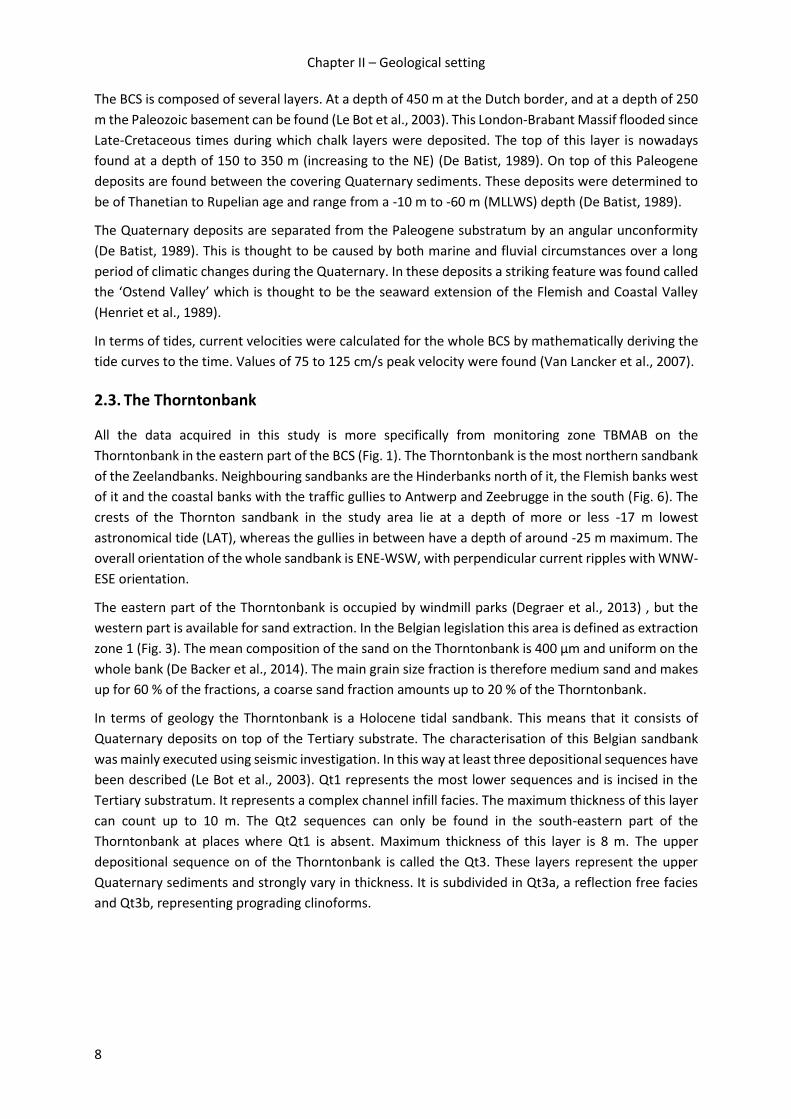
An overview of the calibration results of the Kongsberg EM2040 on RV Simon Stevin is given in table 2.
Table 2. Offset angles in degrees for the calibration of the EM2040 echosounder of RV Simon Stevin.
Offset angles (deg.) Roll Pitch Heading
TX transducer 0.250 0.815 0.240
RX transducer 0.300 -2.220 0.325
GPS antenna 0.200 0.000 0.100
Motion sensor 0.000 0.000 0.000
When everything is calibrated well and every offset is known relative to the zero point of the reference
system, precise location data can be acquired with the on board positioning system. Real Time
Kinematic (RTK) corrections were also received to enhance the precision. Due to the availability of RTK
corrections no tide or draught corrections had to be performed in the processing, as these were already
included in the RTK corrections.
3.2.2. Bathymetry and Seafloor backscatter
The data on board was acquired using the Kongsberg Seafloor Information System software
(Kongsberg Maritime AS, 2007). It has a user friendly interface and visualises the data in real-time.
During all campaigns bathymetry was logged which is automatically calculated by means of the two-
way travel time and the speed of sound in the water. This is not the only thing that is logged. Also the
intensity of the reflected ping is stored. This is commonly known as the backscatter value and is
represented by a value in decibels (dB). The scattering of an emitted ping can occur in the water column
itself or at the seafloor. The SBS is commonly logged together with the bathymetric information and
gives more information about the characteristics of the underground, as it can be used for habitat
mapping and to detect changes in lithology (Lurton, 2002). The on board ADCP of RV Simon Stevin was
switched of due to interference with the WCBS.
3.2.3. Water column backscatter
Due to the large storage capacity needed to store water column data compared to the amount of
information in it (Gee et al., 2012), and the difficulty of processing and calibrating it (Lamarche et al.,
2017), the water column data is mostly not acquired. During the September campaign in this work
however, this data was logged to visualise and process the caused sediment plumes by dredging. The
MBES was set to acquire the data in three sector mode. In this section an overview will be given of the
applications and fields in which WCBS is currently being used.
Water column data is being used in the last decades for the detection of several targets. A detection
in the water column is dependant of two main things: the system and the target. The MBES can be
controlled by changing sonar frequency, vessel speed, acquisition settings, whereas the target that has
to be detected cannot be controlled. Target strength in the water column is dependent on density,
size, orientation, geometry, depth and behaviour of the target itself.
One of the most used applications of water column data from MBES is the detection of gas bubbles.
Imaging of natural gas seepage has already been performed in a lot of instances, mainly for the
detection of methane at seeps in sea (Greinert et al., 2010; Jones et al., 2010; Nikolovska et al., 2008;

Chapter III – Material and methods
16
Ostrovsky et al., 2008; Skarke et al., 2014), methane vents in lakes (Scandella et al., 2016) or mud
volcanoes (Greinert et al., 2006) .
A way of data processing for bubble detection at seeps and black smoker have already been proposed
by Schneider Von Deimling and Papenberg (2012) and Rona et al. (1998). Because of the strong
impedance level between gas bubbles and the water a strong backscatter occurs of the transmitted
acoustic pulse (Greinert, 2008) which makes them fairly easier to detect and process than other
targets. Scandella et al. (2016) gave a more in depth view of the multibeam backscatter physics of the
gas bubbles. By using echo-integration algorithms bubble abundance can be approached instead of
simply counting the individual bubble echoes (Bayrakci et al., 2014), in this way the gas vents can be
quantified. By using split-beam echosounders bubble flow rates have been quantified (Veloso et al.,
2015).
Water column data can also be used for research into submerged vegetation. Mapping the seafloor
vegetation can have benefits for easier environmental monitoring and even enhances the performance
of mine hunting sonars in littoral regions (McCarthy and Sabol, 2000). Echosounders have been proven
useful for environmental monitoring, mainly spatial distribution and biomass analysis of algae (Kruss
et al., 2015, 2011, 2008). Fisherman have used several acoustic methods to enhance their fish gaining.
Sonars can be used for detection of mammals (Pyć et al., 2016), for a density calculation of krill (Cox et
al., 2011) and for normal acoustic observations of several normal sorts of fish (Weber et al., 2009).
Cochrane et al. (2003) and Melvin and Cochrane (2014) go deeper into the physics of using MBES for
fishery research. Other targets studied in the water column are shipwrecks, to detect the least depths
(Wyllie et al., 2015), and water mass differences to determine thermoclines and freshwater influx
(Schneider Von Deimling and Weinrebe, 2014).
More important for this specific work is previous research into the study of sediment plumes using
MBES. The knowledge in this field of science is rather scarce as most research is executed using ADCP
and OBS (Battisto and Friedrichs, 2003). Simmons et al. (2010) showed an early quantitative and
temporal characterisation of sediments in a river mixing interface. By using MBES water column data
and water calibration samples a rough SPM concentration was calculated. However it was stated that
further research was needed in a range of environments and a suitable way had to be found to
calibrate the whole system. This was further applied by Best et al. (2010) to a specific case, namely the
leeside of a low-angle sand dune. Both papers state a workflow that could be applied and propose
further research. However in this work itself the setting is more complex as a detection of the sediment
plume formed by dredging is more difficult as several parameters have to be taken into account.
3.2.4. Sampling
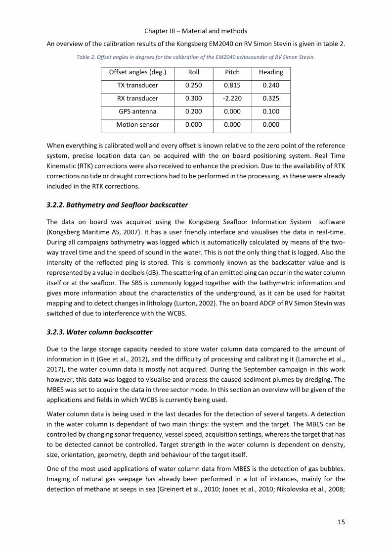
During the March campaign (TBMAB16-310) nine samples were taken on the Thorntonbank. These
were named SPI 1-9 as at that place also Sediment Profile Images (SPI) were taken. Sampling was
performed using a Reineck box corer, with subsampling of the above 15 cm in a plastic bags. Location
and remarks of these samples can be found in table 3.
Three additional samples were taken during the September campaign (TBMAB16-730) along the
dredged track of the Ruyter. This was performed using the same procedure. Info about location of the
samples on the Thorntonbank can be found in table 4.
Chapter III – Material and methods
17
Table 3. Location, date and remarks of the 9 samples acquired during survey TBMAB16-310..
Sample LAT (theorical) LONG
(theorical) Date
Mean Time (UTC)
Remarks IMAGE FILE
NUMBER
SPI 1 51.49071070 2.76368120 12-Apr-16 13:41 Sandy gravel with shells, coarse heterogenous
2552 2553
SPI 2 51.49361122 2.76612752 12-Apr-16 14:02 Sandy gravel with shells, coarse heterogenous
2554 2555
SPI 3 51.49556843 2.76962040 12-Apr-16 14:18 Gravel, soft cobbles of mud
2556 2557
SPI 4 51.49611780 2.77870642 12-Apr-16 14:39 Sand with fragmented shells, homogenous
2558
SPI 5 51.49660047 2.78400605 12-Apr-16 14:49 Sand with fragmented shells, homogenous
2560
SPI 6 51.50009977 2.79099617 12-Apr-16 15:00 Sand with fragmented shells, homogenous
2561 2562
SPI 7 51.50437455 2.80252893 12-Apr-16 15:22
Fine rippled sand, few fragmented shells, homogenous
2563 2564
SPI 8 51.50573652 2.80413288 12-Apr-16 15:34
Fine rippled sand, few fragmented shells, homogenous
2565 2566
SPI 9 51.51114288 2.82219887 12-Apr-16 15:37
Fine rippled sand, few fragmented shells, homogenous
2567 2568
Table 4. Location, date and remarks of the 3 samples acquired during survey TBMAB16-730.
Sample LAT (theorical) LONG
(theorical) Date
Mean Time (UTC)
Remarks IMAGE FILE
NUMBER
R1 51.50445 2.845406 14-Sep-16 10:57 / /
R2 51.50925 2.852442 14-Sep-16 11:29 / /
R3 51.51266 2.863126 14-Sep-16 11:57 / /

Chapter III – Material and methods
18
3.3. Processing of acoustic data
Due to the large extent of the whole dataset, several types of data were combined using multiple
software packages. Qimera and FMGT were used to study the direct impact of dredging (bathymetric
and SBS grids respectively). To study the indirect impact (the suspended sediment plumes caused by
the dredging) FMMidwater, Sonarscope and Voxler were used to visualize the intensity of the plume
in 2D, 3D and even roughly quantify the plume volume. As the processing of water column data in
relation to the specific case of sediment plumes is not common, the methodology in this work will be
an important part and therefore explained more thoroughly.
Firstly all the software processing will be explained with an overview of which features of each program
were used and the to what values the parameters were set. Lastly also the whole processing of the
sand samples to obtain the grain size will be explained.
3.3.1. Processing in Qimera
Qimera is a program developed by QPS (QPS hydrographic and marine software solutions, 2016). It can
be used to process both bathymetry and water column data but was only used for the processing of
the bathymetry in this specific study. The bathymetric raw data consist of all the ‘pings’, which are
points that are georeferenced. The raw data can therefore be simply imagined by a point cloud that
has to be converted to a grid. First step was to import the raw bathymetric data files as they were
acquired in SIS on board of the survey ship. These are the files which have an ‘.all’ extension. After all
the files were imported, the vertical reference separation model was selected. This file was available
at the CSS for the whole BCS. By using the vertical reference separation model all the depth values of
the pings were recalculated from the original depth on the WGS84 ellipsoid to a depth value in Lowest
Astronomical Tide (LAT). Also the real time corrected positions were selected so no additional tide or
draft correction had to be applied as they were already interbedded in the RTK corrections.
After this correction, the point data could be gridded. This was processed with a Combined Uncertainty
and Bathymetry Estimator (CUBE) algorithm (Calder and Wells, 2003). The algorithm focuses on
estimation of true depth, rather than selecting the best soundings. The algorithm uses an estimation
of bathymetry using all the information at hand combined with the uncertainty on that depth estimate.
The use of the CUBE algorithm tremendously improved the speed and efficiency of bathymetric data
processing and provides a quality control needed to optimise surveying (Ladroit et al., 2012). The CUBE
algorithm was applied to all the raw data to provide a dynamic surface. This reduced the amount of
‘faulty’ pings and outliers. The CUBE algorithm settings were ‘shallow water’ as all data acquired was
max 25 m depth LAT, the fixed distance was set on 0.35 m, the number of samples offset 2.00.
Resolution for al grids was set to 1 m in x and y direction as this will give a good equilibrium between
what is needed for discussion of the features and storage capacity needed and calculating time of the
computers on the other side.
At last the pings were visually checked for leftover outliers and if needed flagged out. The eventual
dynamic grids were then definitively exported in asci format to be visualised in Surfer. In the end also
the processed information files where exported in ‘.gsf’ format to be used in FMGT.

Chapter III – Material and methods
19
3.3.2. Processing in FMGeocoder Toolbox (FMGT)
The Fledermaus Geocoder Toolbox module (QPS hydrographic and marine software solutions, 2017)
designed by QPS was used to process the SBS. In this module the files with ‘.gsf’ format were imported
which were already filtered by the CUBE (Calder and Wells, 2003) algorithm and visually corrected
further. No additional processing was required as the SBS mosaic could directly be calculated. The
resolution was set to 1 m and the radius of search to obtain the gridded value was set to 10 m. FMGT
then directly shows the needed memory space. In case the resolution is set to high, the needed mosaic
memory will show up in red and the resolution should be changed accordingly. The end result of the
processing in FMGT is a mosaic with SBS intensity in decibel value.
3.3.3. Processing in FMMidwater
To process the water column data the Fledermaus Midwater module developed by QPS was used (QPS
hydrographic and marine software solutions, 2017). The raw water column data files which have the
‘.wcd’ extension were imported, together with the ‘.all’ files which contain all seafloor pings. In
FMMidwater the water column can be visualized in different ways. It can be visualized as a slice
perpendicular on the survey vessel track like in figure 10.
Visualization can also be performed in stacked view, which is the nadir view along the track of the
vessel (Fig. 10). In all these views the different colours stand for different WCBS values in decibel. In
both figures the sediment plumes can be observed in green as when the dredging vessels were not
followed, so when no sediment is present, these views were plain blue. On the stacked view (Fig. 11)
the seafloor can be observed as a very high scatter (positive decibel values). When looking in fan mode
the seafloor is also detected (the red line in figure 10). Next step is to select the right range to filter out
all the side lobe interference and multiples. This to only have the pure water column itself in the end.
The histogram (Fig. 12) shows that the backscatter values of the sediment plume were filtered out by
trial and error on sight. For the Ruyter track only the backscatter values between -60 to -30 dB were
retained as this represented the first peek in the histogram and corresponded roughly with the
sediment plumes on sight.
At last the remaining backscatter values were exported in text format to be further processed
(additional filtering) and visualized in Voxler. This resulted in a text file with four columns, the first one
the coordinates along x-axis in meter in UTM 31N, the second column the coordinates along y-axis in
meter in UTM 31N, the third axis the depth in meter LAT and the fourth column the backscatter value
in decibels.

Chapter III – Material and methods
20
Figure 10. Screenshot from FMMidwater. Fan view of the water column. The centre blue part with green scatters are the actual water column with the sediment plume in green. The red line at the bottom is the seafloor detection. All the additional green at the sides is due to side lobe interference and multiples. The two black lines show the boundaries between the three sectors in which the water column was recorded.
Figure 11. Screenshot from FMMidwater. Stacked view of the water column. The bottom red part is the seafloor with above the water column containing the sediment plume (in green).
Figure 12. Screenshot of the water column backscatter histogram. The turquoise shows the distribution of the decibel values. The first peak corresponds to the sediment plumes on sight.
22 m
10 m
Relative
count
15 m
100 m
-120 dB
-50 dB
20 dB
-50 dB
20 dB
-120 dB

Chapter III – Material and methods
21
3.3.4. Processing in SonarScope
SonarScope is a software package which is developed by the French Institut Français de Recherche
pour l’Exploitation de la Mer (IFREMER) in France (IFREMER, 2017). The software is programmed in
MATLAB, which makes it very modifiable. The sediment plume was processed by the CSS using the
echo-integration algorithm. In this process a vertical average of backscatter intensity is calculated from
a time angle ring where the specular echo (due to side lobe interference) was already filtered out (Fig.
13). The result of this algorithm is a colour intensity value ranging from 0 to 255 which means that the
original backscatter value is not retained in decibels. The result of the echo-integration can be
visualized for each echogram i.e. ping as a graph in which the echo-integration intensity is plotted in
function of the across distance. A two-dimensional grid can also be made which then shows the
intensity of the sediment plume georeferenced in x and y direction.
From all the water column files the ring in between time angle 0 and 96 was used. This means that the
resulting grids represent the sediment plume generated in the whole water column. Additionally also
echo-integrated grids were computed where not the whole coverage of the water column was used.
The outer 35 degrees on each side of the normal coverage were filtered out as these parts already
have a large degree of interference.
Figure 13. The echo-integration principle. The left upper figure represents the filtering of the side lobe interference and the extraction of the time-angle ring of interest. The left lower graph shows the result of the echo-integration algorithm for each ping. When stacking these pings next to each other, a two-dimensional grid can be made with the plume intensity (right figure) (Figure by courtesy of IFREMER).
.

Chapter III – Material and methods
22
3.3.5. Processing in Surfer 12
All the two-dimensional visualisations were performed using Surfer 12 software (Golden Software Inc.,
2012a). The bathymetric and backscatter grids are just imported as they were exported in the
processing software. Additional data can be visualized on top of these grids such as current files.
Current data at the time of the campaign was retrieved from the website of BMM. This was saved as a
text file with three columns, one with the date, the time and the tide in TAW in centimetre. It is
important to note that the retrieved tide data is from the measuring station ‘De Wandelaar’ which is
at about a distance of 20 kilometres.
Next step in the making of the current vector files was by combining the navigation files of the survey
ship with the current file. The resulting current vector file was therefore prepared by using the time as
connecting factor. The coordinates of the survey ship at the time of each current measurement were
searched and put in a text file with four columns: x coordinates in UTM 31N, y coordinates in UTM
31N, the current orientation in degrees relative to the north in clockwise rotation and the current
velocity in meters per second. This file could then be visualized as a 2-grid vector layer which results in
an overlay with the direction of the arrows indicating the current direction and with their length a
relative measure of the current velocity strength.
Additional methods helped to visualize certain features more clearly. Rather than just importing the
bathymetric and backscatter two-dimensional grids as they were, shaded relief visualizations could be
used to enhance the dredging induced changes. In a shaded relief map the bathymetry is enlightened
from a certain wind direction (in this case the north-western direction), at an angle of 45 degrees with
the horizontal plane. This makes the dredging induced trace more clearly visible, mostly if the dredging
track is perpendicular on the enlightening direction.
Part of the research question was to study the dredging trace and study how fast it changes or becomes
replenished. This is studied by making difference maps between moments in time, represented by the
data acquired at two different campaigns. By making a difference map between the bathymetry of a
campaign before dredging and right afterward, the dredging traces in that time interval can be
visualised. The replenishment of the trace can be studied in the same way by making a difference map
between the situation right after dredging and bathymetry of a campaign afterward.
At last also other data can be plotted such as navigational data of both the dredging vessel, which is to
be found in the EMS data, and the navigational data of the survey vessel. This is performed by adding
as a ‘post’ map and then selecting the right columns of the data file for x coordinates and y coordinates.
3.3.6. Processing in Voxler
Voxler is a software package developed by GoldenSoftware that makes it possible to visualize 3D data
(Golden Software Inc., 2012b). It was used to make a three dimensional model of the already pre-
filtered backscatter data in FMMidwater. The data was converted to voxels, which are a short for
volume pixel, that’s the smallest distinguishable box-shaped part of a three-dimensional image.
First step was to import this data as a text file which consists of four columns like exported in
FMMidwater (X, Y, Z and backscatter value). Once imported an additional filter was applied which
filtered the data further based on the backscatter value. This applied filter was tested using several
ranges, but eventually for all results a filter that only retained the backscatter values in between -40
and -55 was used. As these data were still point data after this operation, the next logical step was to
grid the data. This is executed by the gridder module implemented in Voxler. The voxel geometry was

Chapter III – Material and methods
23
set to 1 m along x and y axis, whereas along z-axis the resolution was set to 0.5 m (due to the smaller
range in depth). The gridding method was an isotropic inverse distance to power algorithm, with power
two. This means that for each value the pings closest to that point will weigh more on the eventual
calculated value than the other pings further away. A one meter radius was used in which minimum 1
ping and maximum 50 pings were used to calculated a grid value.
At last several output geometries were created using several modules. The most important one of
these is the FaceRender module which displays non-interpolated cubes of the gridded input lattice.
Each unit of the grid is visualized as a block with a colour value corresponding to the component value
which is in this case the WCBS value itself. The component value presented are calculated by summing
the values at each of the corner points and dividing them by eight. If one of these neighbouring
components has a null value, the cube will not be displayed. This module actually visualized the
sediment plume as blocks of half a cubic meter, with their colour corresponding to a backscatter value.
The workflow chart as used in Voxler is shown in figure 14. Additionally also other visualization
methods can be used to explore the data more thoroughly like the ‘Contour module’ and the
‘OrthoImage module’. The ‘VolRender module’ was used but did not work out as the volume was not
smooth enough like some other objects in the water column as fish and mines.
Figure 14. Workflow chart of the processing in Voxler. Firstly and additional filter is applied on the already pre-filtered data exported from FMMidwater, then the gridding is performed with then finally the visualisation methods.
3.4. Processing of the sand samples
Firstly the bags with approximately a weight of 2 kg each were oven dried at 40 degrees Celsius to
remove the water content. As the passive plume, processing of the sand samples was firstly performed
by sieving of all the bags on a 1 mm dry sieve. Both fractions, the one higher than 1 mm and the one
smaller than 1 mm were weighed. The fraction smaller than 1 mm was further prepared to then be put
in a Malvern Mastersizer 3000 to be analysed in greater detail. This preparation consisted of an organic

Chapter III – Material and methods
24
matter removal by adding H2O2. (35% solution) and then boiling the mixture until the reaction stopped.
After allowing the sediment to settle again (approximately one day) the liquid was decanted.
Carbonates and/or biogenic silica was not removed as this was not deemed necessary within the
requirements of this study. At last the samples were also treated with Calgon ((NaPO3)6) to make sure
the particles do not stick together when analysed by the Malvern Mastersizer.
Gradistat Version 8.0 (Blott and Pye, 2001) was used to process grain size data. It is freely available and
is mostly used for the rapid analysis of grain size statistics. Several parameters are automatically
calculated such as mean grain size, mode and skewness. Additionally other statistics are calculated
logarithmically (phi units) (Krumbein and Pettijohn, 1938), geometrically (metric units) and
arithmetically using Folk and Ward methods (Folk and Ward, 1957). Also frequency and ternary plots
can be made. It can also provide a description of the textural group and the name of the sediment
(Folk, 1954). The program itself runs in excel which makes everything easy to modify by just pasting
the desired statistics and manipulate them. The raw data is the text file provided from the Malvern
Mastersizer 3000. This file contains general information as operator name, date and time, sample
name, laser obscuration and mode count plus the results of the grain size which is in format of
percentage above certain values. It is only these data that is imported in Gradistat to perform the
processing. As only the general characteristics of all samples were needed, the ‘Multiple Sample Data
Input’ was used to calculate all the parameters.
Additional data was at hand of the grain sizes of the dredged material for all fractions. As this had to
be compared to the in-situ grain size data (of the fraction smaller than 1 mm) all the cumulative
percentages had to be recalculated so that 1 mm corresponded to 100%. By using the grain sizes of
both the in-situ material along the track of the Interballast and this additional grain size data of the
dredged material, the possible fraction that forms the sediment plume can be found.
3.5. Processing of navigation files and EMS
Two main correlations were researched by using the EMS-data files of the dredger and the navigational
data of the survey vessel combined with the echo-integrated grids made in SonarScope. This was
researched by using self-written programs of the CSS, manipulation of all these data and making graphs
and correlation coefficients later-on in Microsoft Office Excel. Two coefficients were calculated, a
Spearman’s ranking coefficient and a Pearson’s correlation coefficient, if possible.
The Pearson’s correlation coefficient, which is mostly symbolised as ‘r’ measures the linear relationship
between two quantitative variables. It is the covariance of the variables divided by the product of their
standard deviations. It can be calculated by the correlation function in Excel. The outcome value lies
always in between -1 and +1, with a total non-correlation at 0 and a positive correlation at +1 and
negative correlation at -1. Some assumptions for the Pearson’s correlation have to be made, with the
most important one here that the variables are approximately normally distributed. This is most of the
time not the case as non-detection of the plume shows extremely low values whereas detection of it
shows high backscatter values. Therefore one should be sure that the plume is relatively well detected
before the relationship between plume intensity and the distance/ time is researched.
The Spearman’s rank correlation, symbolised as the Greek letter ρ (rho) is a non-parametric measure
of rank correlation. It gives a measure of how well the ranked values of both variables correlate to each
other and is therefore less sensitive for outliers than the Pearson’s correlation. Also the variables
shouldn’t necessarily be normally distributed. In this work the Pearson’s correlation coefficient was
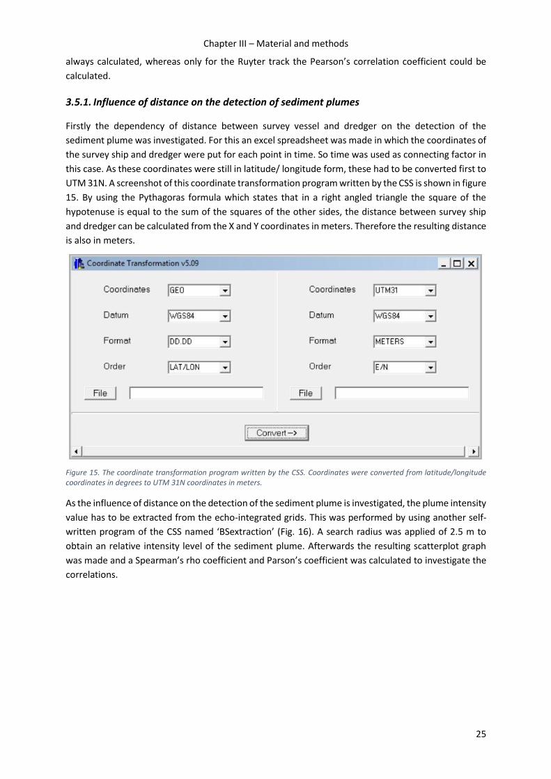
Chapter III – Material and methods
25
always calculated, whereas only for the Ruyter track the Pearson’s correlation coefficient could be
calculated.
3.5.1. Influence of distance on the detection of sediment plumes
Firstly the dependency of distance between survey vessel and dredger on the detection of the
sediment plume was investigated. For this an excel spreadsheet was made in which the coordinates of
the survey ship and dredger were put for each point in time. So time was used as connecting factor in
this case. As these coordinates were still in latitude/ longitude form, these had to be converted first to
UTM 31N. A screenshot of this coordinate transformation program written by the CSS is shown in figure
15. By using the Pythagoras formula which states that in a right angled triangle the square of the
hypotenuse is equal to the sum of the squares of the other sides, the distance between survey ship
and dredger can be calculated from the X and Y coordinates in meters. Therefore the resulting distance
is also in meters.
Figure 15. The coordinate transformation program written by the CSS. Coordinates were converted from latitude/longitude coordinates in degrees to UTM 31N coordinates in meters.
As the influence of distance on the detection of the sediment plume is investigated, the plume intensity
value has to be extracted from the echo-integrated grids. This was performed by using another self-
written program of the CSS named ‘BSextraction’ (Fig. 16). A search radius was applied of 2.5 m to
obtain an relative intensity level of the sediment plume. Afterwards the resulting scatterplot graph
was made and a Spearman’s rho coefficient and Parson’s coefficient was calculated to investigate the
correlations.

Chapter III – Material and methods
26
Figure 16. The backscatter extraction program written by the CSS. This program is used to extract the intensity values of the echo-integrated sediment plume maps.
3.5.2. Influence of time since passing on the detection of sediment plumes
Secondly also the dependency of the time that has passed since the dredging took place and the
passing of the survey vessel, and its influence on the detection of the sediment plume was researched.
This was mainly performed in the same way as in the previous paragraph, by using a self-made program
of the CSS and processing of raw text data files in Excel. A program Vesseltracks (Fig. 17) was used to
search for each position of the dredging vessel for the position of the surveying vessel that was the
closest to that track. From both logs then the time at which they passed at that point was used to
calculate a time difference. Next step was to again extract sediment plume intensity values from the
echo-integrated grids and draw out the scatterplot which shows the plume intensity in function of the
time since passing.
Figure 17. The vessel track comparison program written by the CSS. This program is used to calculate the time difference between two the two nearest data point between the track of the dredger and the survey ship.

27
CHAPTER IV RESULTS
In this chapter all the results are shown starting with the bathymetric and SBS results and the
comparison with before and after the dredging. This is followed by the results from the water column
data in both two and three dimensions. In the last two sections the results of the grain size analysis
and the researched correlations are shown.
4.1. Bathymetry
All the shown grids in the following paragraphs are grids applied to the specific situation of following
TSHD Ruyter. These data most clearly show the dredging induced changes. The resolution of all the
grids shown is 1 meter. All coordinates are in WGS 84 UTM 31N format which means they also show
the scale as these coordinates are expressed in meters. All depth values are expressed with respect to
the Lowest Astronomical Tide (LAT).
4.1.1. Bathymetry right before dredging
The bathymetry that was acquired before TSHD Ruyter was followed in this area shows several
longitudinal depressions in the entire area (the mainly blue fine lines on figure 18). Clear sand dune
crests (red) with their accompanying throughs (blue) can be distinguished which are crosscut by
longitudinal depressions that mainly have a NW-SE orientation or E-W orientation. Note that in the
zoom-in box all crests are undisturbed.
Figure 18. Bathymetry of a part of the Thorntonbank which shows the general outline of this particular area with an outlet in which later-on the TSHD will pass.
4.1.2. Bathymetry directly after dredging
The bathymetric situation moments after the dredging of TSHD Ruyter can be observed in figure 19.
Important is the fact that a new longitudinal depression is to be observed (encircled area on figure 19)
which clearly crosscuts the sand crests which were previously undisturbed in figure 18. This
longitudinal depression is even more distinctive on a shaded relief grid on which the feature is depicted

Chapter IV - Results
28
as enlightened from the north-eastern corner under a vertical angle of 45 degrees with the horizon
(Fig. 20).
Figure 19. Bathymetry of the track following the Ruyter (TBMAB16-730). The encircled in the zoom-in box is a depression line which crosses the sand crests. In the south-western part of the track, several of these lines can be differentiated.
Figure 20. Shaded relief grid of the track following the Ruyter (TBMAB16-730). The grid is enlightened from the northwest, under a degree of 45° with the horizon. The depression features are best visualised on this grid, as again in the zoom-in one track can be visualised whereas in the southwestern part of all the data a hot spot of depressions can be found.
The depth of the depression can be estimated by calculating a difference map between bathymetric
charts of two different moments in time. The calculated difference between the bathymetric situation
right before and right after dredging shows that the depressions mainly have a depth ranging from
0.20 m to 0.30 m (greenish to yellow colour) (Fig. 21). At some points the depression even adds up to
0.50 m. At the outer sides of the grid the differences add up to more than 0.5 m (red and greenish
colour). The width of the depression was measured in Surfer itself by counting about two pixels, which

Chapter IV – Results
29
means the width is one to two meters. This has also been confirmed by making a cross section in
Qimera.
Figure 21. Difference grid of the Ruyter track (1m resolution). Bathymetry of the September campaign (TBMAB16-730) was subtracted from the previous April campaign bathymetry (TBMAB16-310). Therefore the positive difference is sand that was dredged.
4.1.3. Bathymetry two months after dredging
At last also the bathymetry that was surveyed two months after the studied dredging can be shown
(Fig. 22). This shows that the sand crests are replenished again, the previous depressions on the crests
are not visible anymore. In the through some bit of the dredging track can still be observed.
Figure 22. Bathymetry of the Thorntonbank two months after the studied dredging took place. The sand crests are again replenished although the depression in the troughs remain
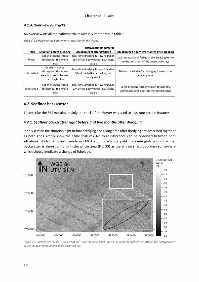
Chapter IV - Results
30
4.1.4. Overview all tracks
An overview off all the bathymetric results is summarized in table 5.
Table 5. Overview of the bathymetric results for all the tracks.
4.2. Seafloor backscatter
To describe the SBS mosaics, mainly the track of the Ruyter was used to illustrate certain features.
4.2.1. Seafloor backscatter right before and two months after dredging
In this section the situation right before dredging and a long time after dredging are described together
as both grids simply show the same features. No clear difference can be observed between both
situations. Both the mosaics made in FMGT and SonarScope yield the same grids and show that
backscatter is almost uniform in the whole area (Fig. 23) as there is no sharp boundary somewhere
which should implicate a change of lithology.
Figure 23. Backscatter mosaic of a part of the Thorntonbank which shows the uniform backscatter. Also in the enlarged part of our study area nothing is to be observed yet.
Track Situation before dredging Situation right after dredging Situation half hour/ two months after dredging
Ruyter
Lot of dredging traces
throughout the whole
area
Real-time dredging furrow found on
85% of the bathymetric line, clearly
visible
Data not available/ fading of the dredging furrow
on the crest, rest of the depression stays
Bathymetry (in Qimera)
Dredging traces
throughout the whole
area, but less to be seen
than Ruyter line
Real-time dredging furrow found on
5% of the bathymetric line, but
poorly visible
Data not available/ no dredging furrow to be
seen anymoreInterballast
Schotsman
Lot of dredging traces
throughout the whole
area
Real-time dredging furrow found on
50% of the bathymetric line, clearly
visible
Same dredging furrow visible/ bathymetry
unavailable (track outside monitoring zone)

Chapter IV – Results
31
4.2.2. Seafloor backscatter directly after dredging
The backscatter mosaic of the situation directly after dredging however reveals more interesting
things. Backscatter grids were performed using both FMGT and Sonarscope. Figure 24 shows the
resulting SBS grid made in FMGT whereas figure 25 shows the resulting backscatter grid made using
the SonarScope software. The small depression lines can once again be differentiated (the small thin
line of high scattering values).
However there is a remarkable fact when comparing the FMGT and SonarScope grid. Although the
resolution of both grids is one meter, there is a difference to be observed between figure 24 and figure
25. On figure 25 the depression is accompanied with a ‘halo’ of high scatters on the south-eastern side.
This ‘halo’ consists of scatters which yield a value between -32 to -40 dB and is found throughout the
whole track next to the depression line (Fig. 20). This ‘halo’ is not visible on the FMGT mosaic (Fig. 24).
Figure 24. Backscatter grid of the Ruyter track (TBMAB16-730) made using FMGT.
Figure 25. Backscatter grid of the Ruyter track (TBMAB16-730) made using Sonarscope. Note the ‘halo’ of high scatters at the south-eastern side of the depression line.

Chapter IV - Results
32
4.2.3. Overview of all tracks
An overview of all the backscatter data of all tracks processed in this study and their results is shown
in table 6 and table 7. It shows that the ‘halo’ is not to be observed on the FMGT grids, whereas they
are observed directly after dredging on the SonarScope grids.
Table 6. Overview of the seafloor backscatter results for all the tracks in FMGT.
Table 7. Overview of the seafloor backscatter results for all the tracks in SonarScope.
Track Situation before dredging Situation right after dredging Situation half hour/ two months after dredging
Seafloor backscatter (in FMGT)
Data not available/ nothing special to be seen,
some interferenceRuyter
Interballast Uniformous backscatter
Higher backscatter in the real-time
dredging furrow, accompanied by a
lower backscattervalues next to it,
no halo
Data not available/ nothing special to be seen
Uniformous backscatter,
in the NE slightly higher
backscatter overall
Higher backscatter in the real-time
dredging furrow, accompanied by a
lower backscattervalues next to it,
no halo
Nothing special to be seen / nothing Special to be
seen
Higher backscatter in the real-time
dredging furrow, accompanied by a
lower backscattervalues next to it,
no halo
Uniformous backscatter,
slightly higher backscatter
in the centre of the track
Schotsman
Track Situation before dredging Situation right after dredging Situation half hour after dredging/ two months
Seafloor backscatter (in SonarScope)
Uniformous backscatter,
slightly higher backscatter
in the centre of the track,
no halo
Ruyter
Uniformous backscatter,
in the NE slightly higher
backscatter overall, no
halo
Higher backscatter in the real-time
dredging furrow, accompanied by a
lower backscattervalues next to it,
halo
Uniformous backscatter,
no haloInterballast
Schotsman
Higher backscatter in the real-time
dredging furrow, accompanied by a
lower backscattervalues next to it,
halo
Not available/ no halo visible
Not available/ no halo visible
Half an hour later, the halo of higher backscatter
values is gone / no halo visible
Higher backscatter in the real-time
dredging furrow, accompanied by a
lower backscattervalues next to it,
halo

Chapter IV – Results
33
4.3. Water column backscatter
Water column processing mainly resulted in the visualization of it in two dimensions and possibly in
three dimensions. A calculation of sediment plume volume was performed using the amount of
sediment plume voxels, this will give a rough quantification of the sediment plume. Firstly the results
of processing in FMMidwater and SonarScope will be shown, followed by the three dimensional
visualizations in Voxler.
4.3.1. Two-dimensional results
The water column was processed using two software packages. By using the echo-integration
algorithm in SonarScope a grid could be made with the plume intensity. This intensity is not retained
in original decibel value but converted to a colour value between 0 and 256. The results of this echo-
integration for the plume of the Ruyter can be observed in figure 26. The centre part of the grid shows
high plume intensities whereas at the border blue bands of low intensity are found. The plume
intensity value diminishes from centre to the border of the footprint.
Figure 26. Intensity of the sediment plume resulting from the SonarScope echo-integration algorithm. All sectors of the water column were used. The original decibel backscatter values are not retained.

Chapter IV - Results
34
4.3.2. Three-dimensional results
To better visualize the made three dimensional model, only a part of the sediment plume caused by
TSHD Ruyter will be shown in the following figures. In this case the data from line 31 was used.
Figure 27 shows the first step in making the model, namely the raw pre-filtered backscatter values
ranging from -60 to -30 decibels, exported from FMMidwater. Therefore it is important to note that all
the values that are observed are already the sediment plume itself, as most of the backscatter values
of the water column were already filtered out in FMMidwater.
Figure 28 shows the results of the VolumeRender module that was applied on the gridded values. The
resulting model shows the sediment plume in a transparent way. In this way it can be found where the
higher intensities are inside the sediment plume itself. The question in this case is if these higher values
ranging from -49 to -40 decibels are related to a denser sediment plume (higher sediment
concentration) or related to fish which cause the higher values.
The results of the FaceRender module are shown in figure 29. This shows the sediment plume modelled
in blocks of half a cubic meter (1 m resolution in x and y, 0.5 m resolution in z direction). The colour
once again shows the mean backscatter value for that block, which are here at the outside in the range
of -55 to -52 decibels. In the FaceRender module itself an approximate calculation was shown of the
volume of voxels. This results in an approximate volume of 2003 m³ for line 31 of the data of following
the Ruyter. In analogy this was calculated for the whole track (so all lines from the Ruyter track). This
resulted in a volume of 48520 m³.
Figure 27. The raw backscatter values from a part of the sediment plume caused by TSHD the Ruyter. Colours correspond to the backscatter values in decibel, which are mainly in the range of -52 to -55 decibels.

Chapter IV – Results
35
Figure 28. Volume render of the sediment plume caused by TSHD the Ruyter. In the inside of the plume high scattering values are to be found (ranging from -49 to -40 decibels).
Figure 29. Face render of the sediment plume caused by TSHD the Ruyter. The sediment plume is visualised as built up from blocks of half a cubic meter (one meter resolution in x and y, half a meter resolution along z axis. Their intensities is again
show by their colour (mainly purple and blue on the outside).

Chapter IV - Results
36
4.4. Influence of time or distance between vessels on the plume intensity
4.4.1. Results for TSHD Ruyter
The first of the two key correlations that were researched was to research if the distance between
dredger and survey ship had an influence on the intensity of the sediment plume (Fig. 30). It shows a
cluster of points with the majority of plume intensities ranging in between 60 and 100. The distance at
which the Ruyter was followed was always in between 400 and 600 m. Additionally also a Spearman’s
rho rank correlation coefficient and a Pearson’s correlation coefficient was calculated. These were -
0.20 and -0.14 respectively.
Figure 30. Plume intensity in function of the distance between TSHD the Ruyter and RV Simon Stevin.
The second correlation investigated was to investigate what the influence was of the time since passing
on the intensity of sediment plumes. The resulting scatterplot of this can be found in figure 31. The
time difference was as in the previous correlation constant, ranging in between 900 and 1200 seconds
that have passed since the dredging ship passed. Intensities of the sediment plume lie mainly in
between 60 and 110, with one outlier around 40. For this correlation the Spearman’s rho rank
correlation coefficient was -0.41, and the Pearson’s r correlation could not be calculated as the time
values were not normally distributed, which was one of the requirements of calculating a Pearson’s r
coefficient.
Figure 31. Plume intensity in function of the distance between TSHD the Ruyter and RV Simon Stevin.
0
50
100
150
0 100 200 300 400 500 600 700
plu
me
inte
nsi
ty
(dim
ensi
on
less
)
distance between vessels (m)
Correlation distance between vessels vs. plume intensity caused by TSHD Ruyter
0
50
100
150
0 200 400 600 800 1000 1200 1400
plu
me
inte
nsi
ty
(dim
ensi
on
less
)
time (s)
Correlation time between passing of the vessels and plume intensity caused by TSHD Ruyter

Chapter IV – Results
37
4.4.2. Overview results for the other tracks
The results from the other tracks (Table 8) show that for the Interballast track nothing correlates at all,
whereas for the Schotsman higher Spearman’s correlation coefficients are found than those shown for
the Ruyter track. As in the discussion time range and distance range will be of an importance, these
are also given in table 8. Only for the distance – plume intensity correlation of the Ruyter track a
Pearson’s coefficient was calculated as in other cases, either the distance or time or plume intensity
was not normally distributed.
Table 8. Overview of the correlation coefficient results for all tracks.
4.5. Grain size analysis
The grain size analysis of the fraction smaller than 1 mm of the samples ‘SPI1-9’, the samples that were
taken on the Thorntonbank in the April campaign, show that the sand fraction is dominantly medium
sand. A brief summary of some selected statistical parameters is given in table 9Table 9.
Table 9. Grain size results of the fraction less than 1 mm from the samples on the Thorntonbank.
Results of the grain size analyses of the samples taken in the September campaign along the track of
TSHD Interballast are shown in table 10. Table 11 shows the mean grain size distribution of the dredged
material (46 samples) on the Thorntonbank that in the end is used in building materials. This data was
provide by the CSS. In both cases the highest increase in cumulative percentage can be found in the
fraction between roughly 250 to 500 µm which means that the main grain size is medium sand (Fig.
32). However the dredged material also appears to be coarser overall. This is confirmed by the grain
size at 50 percent (D50). D50 for the in-situ seafloor material is 364.33 µm whereas it is 397.99 µm for
the dredged material.
Track Correlation Spearman's coefficient Pearson's coefficient Time range (s) Distance range (m)
Distance - plume intensity -0.20 -0.14 400-600
Time - plume intensity -0.41 not normally distributed 850-1200
Distance - plume intensity 0.01 not normally distributed 200-400
Time - plume intensity 0.04 not normally distributed 250-450
Distance - plume intensity -0.60 not normally distributed 150-550
Time - plume intensity -0.36 not normally distributed 0-550
Ruyter
Interballast
Schotsman
SAMPLE NAME: SPI 1 SPI 2 SPI 3 SPI 4 SPI 5 SPI 6 SPI 7 SPI 8 SPI 9
MEAN 360.18 304.21 370.24 384.27 406.16 389.71 393.80 361.51 385.07
SORTING 1.51 1.60 1.43 1.38 1.39 1.37 1.39 1.36 1.46
SKEWNESS -0.03 -0.09 -0.02 0.00 0.00 0.00 -0.01 -0.01 0.03
KURTOSIS 0.96 1.04 0.93 0.96 0.95 0.96 0.95 0.95 0.95
D10 (mm): 209.39 163.17 231.32 253.43 265.92 257.97 256.51 242.77 238.76
D50 (mm): 361.83 308.39 371.26 384.20 406.71 389.66 394.06 361.90 383.41
D90 (mm): 608.73 536.83 586.00 579.75 620.81 584.72 600.87 540.38 634.83
(D90 / D10) (mm): 2.91 3.29 2.53 2.29 2.33 2.27 2.34 2.23 2.66
(D90 - D10) (mm): 399.34 373.66 354.68 326.32 354.89 326.75 344.35 297.61 396.07
(D75 / D25) (mm): 1.78 1.87 1.66 1.56 1.58 1.55 1.58 1.54 1.70
(D75 - D25) (mm): 210.31 195.11 190.64 172.22 186.39 173.22 181.61 157.20 205.46
Well
Sorted
Medium
Well
Sorted
Medium
Moderately
Well Sorted
Medium
SEDIMENT NAME:
Moderately
Well Sorted
Medium Sand
Moderately
Well Sorted
Medium
Moderately
Well Sorted
Medium
Well
Sorted
Medium
Well
Sorted
Medium
Well
Sorted
Medium
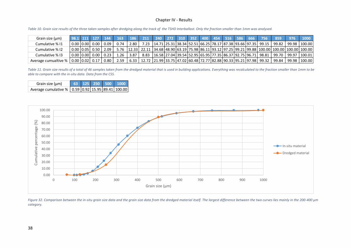
Chapter IV - Results
38
Table 10. Grain size results of the three taken samples after dredging along the track of the TSHD Interballast. Only the fraction smaller than 1mm was analysed.
Table 11. Grain size results of a total of 46 samples taken from the dredged material that is used in building applications. Everything was recalculated to the fraction smaller than 1mm to be able to compare with the in-situ data. Data from the CSS.
Figure 32. Comparison between the in-situ grain size data and the grain size data from the dredged material itself. The largest difference between the two curves lies mainly in the 200-400 µm category.
Grain size (µm) 98.1 111 127 144 163 186 211 240 272 310 352 400 454 516 586 666 756 859 976 1000
Cumulative % I1 0.00 0.00 0.00 0.09 0.74 2.80 7.23 14.71 25.31 38.34 52.51 66.25 78.17 87.38 93.66 97.35 99.15 99.82 99.98 100.00
Cumulative % I2 0.00 0.05 0.50 2.09 5.76 12.33 22.11 34.68 48.90 63.19 75.98 86.11 93.12 97.25 99.21 99.88 100.00 100.00 100.00 100.00
Cumulative % I3 0.00 0.00 0.00 0.23 1.26 3.87 8.83 16.58 27.04 39.54 52.95 65.95 77.35 86.37 92.75 96.71 98.81 99.70 99.97 100.01
Average cumualtive % 0.00 0.02 0.17 0.80 2.59 6.33 12.72 21.99 33.75 47.02 60.48 72.77 82.88 90.33 95.21 97.98 99.32 99.84 99.98 100.00
Grain size (µm) 63 125 250 500 1000
Average cumulative % 0.59 0.92 15.95 89.41 100.00
0.00
10.00
20.00
30.00
40.00
50.00
60.00
70.00
80.00
90.00
100.00
0 100 200 300 400 500 600 700 800 900 1000
Cu
mu
lati
ve p
erce
nta
ge (
%)
Grain size (µm)
In-situ material
Dredged material

39
CHAPTER V DISCUSSION
5.1. Evolution of the tracks on bathymetry
The depressions found on the bathymetric grids are clearly caused by the TSHD. When the navigation
data is plotted on the shaded relief map, one particular trace stands out that matches the track of
TSHD Ruyter. This can be observed in figure 33 where the navigation data of the Ruyter (in green)
corresponds to a clear longitudinal depression. The approximate dredged depth of about 0.2 to 0.3 m
corresponds to the typical amount of sand that is scraped from the bottom by a TSHD (Mills and Kemps,
2016). The track was not yet visible on the situation before dredging (Fig. 18). Moreover the width of
the track is in the same order of magnitude as the width of the suction head of a TSHD. In the specific
case of the Ruyter, the width of the suction head is not known, but the diameter of the suction pipe is
0.65 m (Dredgepoint, 2017a). The suction head will therefore be approximately 1 to 2 m wide and this
is almost the same and at least in the same order of magnitude as the width of the longitudinal
depression.
The estimation of how well the dredging furrow was observed in table 5 was performed in the same
way as in figure 33. The data of the Ruyter represents the dredging induced changes the best as along
that track almost 85% of the real-time dredging furrow was captured. The data acquired following the
Interballast only shows an estimated 15% of the dredging track which makes it difficult to study the
dredging induced consequences as to be observed on SBS and possibly also the WCBS as the surveyed
track was further of the dredged furrow. Also only 50% of the dredging track was captured when
following TSHD Schotsman which makes it also less ideal to be studied.
Figure 33. Plot of the navigation data on the shaded relief map following TSHD Ruyter. The red crosses form the track of RV Simon Stevin whereas the green crosses form the track of TSHD Ruyter. One clear dredging trace matches the navigation data of TSHD Ruyter

Chapter V - Discussion
40
As for the fading of the dredging track this could just be due to the instability of the crest together with
the influence of currents. Previous research already showed that the sand crests move and generally
become lower due to the extraction in that area (Roche et al., 2017)). Sand does not replenish as once
again recent publications of the CSS showed (Degrendele et al., 2010; Roche et al., 2013), but small
depressions appear to fade probably due to current.
It can therefore be proven that the real-time impact of dredging is recorded and therefore the
backscatter data acquired from the water column and seafloor can be investigated to research what
the consequences of dredging give on these type of data.
5.2. Impact and evolution on seafloor with SBS
Firstly the difference between the backscatter grid made in FMGT and the one made in SonarScope
has to be explained. On the grid made using SonarScope a clear ‘halo’ of high scatters was observed
next to the real-time dredging trace. This ‘halo’ is not observed on the FMGT grid. Both grids have a
one meter resolution so this difference is not caused by a different resolution. As the ‘halo’ was also
observed on the SonarScope grids next to the real-time dredging track following TSHD Interballast and
TSHD Schotsman, it can firstly be said that the ‘halo’ of high scatters really is there and is caused by
the dredging operation itself. The question that arises then is why this ‘halo’ is not visible on the grid
made in FMGT.
As stated in the report of the GEOHAB working group about calibration and processing of SBS data,
most post-processing software’s implement a long processing chain to reach the resulting backscatter
mosaic (Lurton and Lamarche, 2015). This chain of processing the raw data, going from decoding of
raw measurements to the whether or not correcting for static and time-varying gain, source level and
transmit and receive level, propagation losses, correcting for ensonified areas or volumes and/or
correcting for angular dependence can be the cause of this difference between the two grids.
As in FMMidwater only the resolution and search radius have to be set, one does not always know
what goes on when the backscatter mosaic is created. Therefore further research is needed into these
specific processing chains of both software packages as it could be important in this case, and in the
general case of processing SBS. Especially in the case of the research and attempts in the recent years
to calibrate the SBS (Lurton and Lamarche, 2015) to be able to compare results acquired with different
systems, this proves once again that also software processing can lead to large differences in outcome
grids, even when using the same raw data.
For the cause of the observed ‘halo’ several hypothesis were made. First of all it should be noted that
this ‘halo’ is a really temporary thing which is clearly dredging induced and which also fades a half hour
after dredging. One hypothesis that was discussed with members of the CSS to explain this onset of
higher scatters and the following fading afterwards, was the possibility of temporal relative enrichment
of the coarse fraction (shells and gravel) due to the finer fraction going temporarily into suspension
because of the dragging of the suction head on the seafloor. The drag head of the TSHD causes
turbulence which leads to a sediment plume and temporarily less fine sediment on the seafloor. The
following disappearance of the ‘halo’ could then be explained by the settlement of the sediment plume
again which will lead to an again normal SBS value.
As shown in the next section also the sediment plume will be gone, so the sediment cloud settles in
more or less the same place and is not transported with the current, additional proof of this is shown
by the vector map (Fig. 34). This shows that the sediment plume was transported for several meters

Chapter V – Discussion
41
by the current, although after calculations with the current speed at hand and the mean time
difference between the dredging operation and the actual surveying, the sediment plume should be
way of the place where it was detected here. The mean time is around 1000 seconds, the mean current
around 0.4 m/s which means that the cloud should have drifted off for 400 m whereas here it only
drifted off for 50- 100 meter. A possible explanation for this is that the plume is stable, which means
that it is not very much influenced by the current. This would also fit in the hypothesis of the ‘halo’,
which states that the sediment plume has to settle at more or less the same place in order to explain
the disappearance of the ‘halo’ half an hour after dredging.
Figure 34. Plume intensity along TSHD Ruyter track. The vectors show the current direction. The black crosses show the navigation data of the dredger. Current info retrieved for measuring station ‘De Wandelaar’ (Meetnet Vlaamse Banken, 2017).
5.3. Visualization of the sediment plumes
Processing of the water column resulted in clear representations of the water column in both two
dimensions and three dimensions. During the processing and interpretation several problems were
encountered and advantages and disadvantages were found which will be discussed in the next
section.
5.3.1. Quality of the visualizations in two and three dimensions
The resulting grids of the echo-integration in SonarScope give a more or less decent representation of
the sediment plume intensity in two dimensions although insights were gathered in some flaws
incorporated in it. Figure 26 showed the echo-integration of almost the whole water column (upper
96 percent). What stands out on that grid were the bands of lower plume intensity at the sides of the
track with a clear abrupt shift in plume intensity value. This shift was hypothesised to have three
possible causes.
Firstly one can think of an actual decrease of plume intensity, this would mean that the sediment plume
was perfectly captured and the blue colour values at the sides would then actually mean a non-
detection of the sediment plume. However this would be a lot of coincidence. It would mean that
throughout the whole track the sediment plume was followed and recorded perfectly. It would be
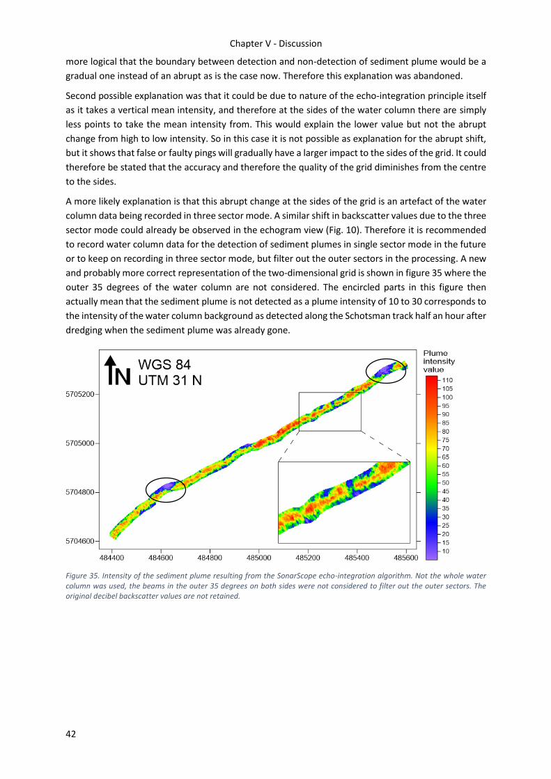
Chapter V - Discussion
42
more logical that the boundary between detection and non-detection of sediment plume would be a
gradual one instead of an abrupt as is the case now. Therefore this explanation was abandoned.
Second possible explanation was that it could be due to nature of the echo-integration principle itself
as it takes a vertical mean intensity, and therefore at the sides of the water column there are simply
less points to take the mean intensity from. This would explain the lower value but not the abrupt
change from high to low intensity. So in this case it is not possible as explanation for the abrupt shift,
but it shows that false or faulty pings will gradually have a larger impact to the sides of the grid. It could
therefore be stated that the accuracy and therefore the quality of the grid diminishes from the centre
to the sides.
A more likely explanation is that this abrupt change at the sides of the grid is an artefact of the water
column data being recorded in three sector mode. A similar shift in backscatter values due to the three
sector mode could already be observed in the echogram view (Fig. 10). Therefore it is recommended
to record water column data for the detection of sediment plumes in single sector mode in the future
or to keep on recording in three sector mode, but filter out the outer sectors in the processing. A new
and probably more correct representation of the two-dimensional grid is shown in figure 35 where the
outer 35 degrees of the water column are not considered. The encircled parts in this figure then
actually mean that the sediment plume is not detected as a plume intensity of 10 to 30 corresponds to
the intensity of the water column background as detected along the Schotsman track half an hour after
dredging when the sediment plume was already gone.
Figure 35. Intensity of the sediment plume resulting from the SonarScope echo-integration algorithm. Not the whole water column was used, the beams in the outer 35 degrees on both sides were not considered to filter out the outer sectors. The original decibel backscatter values are not retained.
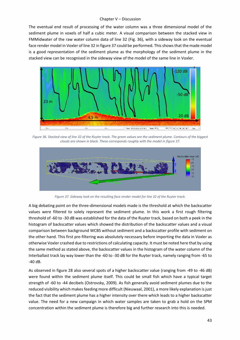
Chapter V – Discussion
43
The eventual end result of processing of the water column was a three dimensional model of the
sediment plume in voxels of half a cubic meter. A visual comparison between the stacked view in
FMMidwater of the raw water column data of line 32 (Fig. 36), with a sideway look on the eventual
face render model in Voxler of line 32 in figure 37 could be performed. This shows that the made model
is a good representation of the sediment plume as the morphology of the sediment plume in the
stacked view can be recognised in the sideway view of the model of the same line in Voxler.
Figure 36. Stacked view of line 32 of the Ruyter track. The green values are the sediment plume. Contours of the biggest clouds are shown in black. These corresponds roughly with the model in figure 37.
Figure 37. Sideway look on the resulting face render model for line 32 of the Ruyter track.
A big debating point on the three-dimensional models made is the threshold at which the backscatter
values were filtered to solely represent the sediment plume. In this work a first rough filtering
threshold of -60 to -30 dB was established for the data of the Ruyter track, based on both a peek in the
histogram of backscatter values which showed the distribution of the backscatter values and a visual
comparison between background WCBS without sediment and a backscatter profile with sediment on
the other hand. This first pre-filtering was absolutely necessary before importing the data in Voxler as
otherwise Voxler crashed due to restrictions of calculating capacity. It must be noted here that by using
the same method as stated above, the backscatter values in the histogram of the water column of the
Interballast track lay way lower than the -60 to -30 dB for the Ruyter track, namely ranging from -65 to
-40 dB.
As observed in figure 28 also several spots of a higher backscatter value (ranging from -49 to -46 dB)
were found within the sediment plume itself. This could be small fish which have a typical target
strength of -60 to -44 decibels (Ostrovsky, 2009). As fish generally avoid sediment plumes due to the
reduced visibility which makes feeding more difficult (Nieuwaal, 2001), a more likely explanation is just
the fact that the sediment plume has a higher intensity over there which leads to a higher backscatter
value. The need for a new campaign in which water samples are taken to grab a hold on the SPM
concentration within the sediment plume is therefore big and further research into this is needed.
23 m
4.5 m
-50 dB
20 dB
-120 dB

Chapter V - Discussion
44
5.3.2. The difficulty of processing water column data with sediment plumes
First of all it should be noted that processing of the water column takes a lot of storage capacity relative
to normal bathymetric data. One minute of water column data recorded along track on the
Thorntonbank takes around 25 Mb. This means that one hour of recording already adds up to 1.5 Gb.
This led to problems when processing the raw point data, with sometimes calculating times of several
minutes when processing one line at a time. Especially when visualizing all the raw data Voxler crashed
most of the times. It was only by pre-filtering to reduce the size of the files by an order magnitude that
the several modules in Voxler could be applied to the data to be further processed. This problem can
be solved in two ways. Either supercomputers have to be used with higher calculating and visualising
capacities or the water column data acquiring software needs an implementation to reduce or
compress the water column data.
The biggest minor side of the two-dimensional grids in SonarScope that show the plume intensity is
the fact that the echo-integration algorithm in SonarScope does not retain the original backscatter
value in decibels. It recalculates the values to a colour intensity value which is actually loss of
information. It would therefore be an interesting feature if the developers update the software to
make sure it retains the original backscatter value. In that way also the influence of scatters in the
water column on the SBS can be investigated directly.
One last big problem was the inability of FMMidwater to automatically select the right range for each
echogram. When in fan view (Fig. 38) this range can be manually set to specifically match that
echogram. However this range will not be the right range for every echogram as the water column
height is never constant due to sand dunes and ripples. This will lead to a situation in stacked view as
observed in figure 39 where in a part of the water column the range will be set to high which leads to
plume and water column data being lost when exporting. At other parts the range will be set to low,
which means that parts of the seafloor and side lobe interference will be incorporated in the exported
data.
In all the models of this work the range was set high enough so not to incorporate the seafloor and
side lobe interference. This means that the models made in Voxler miss some small lower part of the
water column data and that the volume calculations in the face render module are actually
underestimated. An automatic detection of the right range for each echogram would therefore be a
useful feature in the future.
Figure 38. Echogram of water column with a good range set to filter out side lobe interference. The red line is the boundary, only the coloured part is retained.
20 m -50 dB
20 dB
-120 dB
100 m

Chapter V – Discussion
45
Figure 39. The accompanying stacked view of figure 38. Only the parts above the grey zone were retained. The thin central black line corresponds to echogram shown in figure 38.
5.4. Possible grain size of the sediment plume
Figure 32 showed the difference in grain size distribution between what is available at the seafloor on
the Thorntonbank, and the eventual grain size of the dredged material. Although less data of this
dredged material was available (only cumulative percentages of five grain sizes) a cautious statement
can be made. As the difference between the cumulative percentages in figure 32 becomes bigger in
between a grain size of approximately 175 µm and 250 µm, this could possibly indicate the grain size
of the SPM in the water column, being medium sand.
It will be important in future research to have more extended grain size data of the dredged material
to exactly compare it and calculate what the fraction is of the SPM. Maybe more accurate would be
the direct measurement of SPM concentration in the water column using water samples. When this
concentration is known it can be further researched what the influence is of the concentration of that
actual suspended fraction on the backscatter values.
5.5. Impact of measurement conditions on results
First of all it should be noted that the effective capture of the sediment plume is a prerequisite to
research the correlation between distance/time and plume intensity. A non-detection of sediment
plume (intensity ranging from 5 to 30) will only add random water column noise data points. Therefore
when looking to the two-dimensional plume intensity grid only the data from the Ruyter track was
considered and only these calculated coefficients should be used. This because only along that track
the sediment plume was captured along the whole water column.
The researched dependence of distance between survey and dredging vessel and the plume intensity
for the Ruyter track shows that in that case it seems to not matter much for the intensity of the
sediment plume if the survey vessel navigates close by or further away from the dredger. With a
Pearson’s correlation coefficient of -0.14 and a Spearman’s rho rank correlation coefficient of -0.20 an
almost non-correlation is proven. A fixed or varying distance between both vessels will have no
implications on the acquired backscatter strength value of the sediment plume.
-50 dB
20 dB
-120 dB
20 m
10 m

Chapter V - Discussion
46
The dependence of time since passing between dredger and survey vessel versus the intensity of the
sediment plume shows a moderate negative Spearman’s rho rank correlation coefficient of -0.41. This
means that the longer the time in between dredging and surveying, the lower the intensity of the
plume will be. This implicates that the time since passing of dredger before detection by the survey
ship has a ‘moderate’ relation to the plume intensity. This is in one way also logical as this is probably
due to the sediment plume that disperses with a lower backscattering of the SPM as consequence.
Combining both points shows that there is a certain flexibility in detecting sediment plumes. Distance
can vary in some way, there is no need to always stay at a certain fixed space behind the dredger. As
for time there is a slightly higher dependence but this data showed that even after 1000 seconds the
sediment plume is still visible. All this shows that the sediment plume has a certain consistency and is
more or less stable and does not change or disperses that fast.
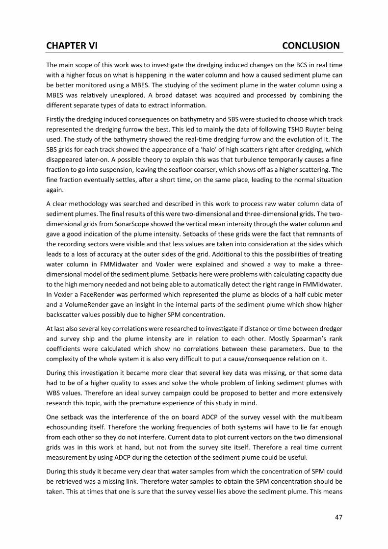
47
CHAPTER VI CONCLUSION
The main scope of this work was to investigate the dredging induced changes on the BCS in real time
with a higher focus on what is happening in the water column and how a caused sediment plume can
be better monitored using a MBES. The studying of the sediment plume in the water column using a
MBES was relatively unexplored. A broad dataset was acquired and processed by combining the
different separate types of data to extract information.
Firstly the dredging induced consequences on bathymetry and SBS were studied to choose which track
represented the dredging furrow the best. This led to mainly the data of following TSHD Ruyter being
used. The study of the bathymetry showed the real-time dredging furrow and the evolution of it. The
SBS grids for each track showed the appearance of a ‘halo’ of high scatters right after dredging, which
disappeared later-on. A possible theory to explain this was that turbulence temporarily causes a fine
fraction to go into suspension, leaving the seafloor coarser, which shows off as a higher scattering. The
fine fraction eventually settles, after a short time, on the same place, leading to the normal situation
again.
A clear methodology was searched and described in this work to process raw water column data of
sediment plumes. The final results of this were two-dimensional and three-dimensional grids. The two-
dimensional grids from SonarScope showed the vertical mean intensity through the water column and
gave a good indication of the plume intensity. Setbacks of these grids were the fact that remnants of
the recording sectors were visible and that less values are taken into consideration at the sides which
leads to a loss of accuracy at the outer sides of the grid. Additional to this the possibilities of treating
water column in FMMidwater and Voxler were explained and showed a way to make a three-
dimensional model of the sediment plume. Setbacks here were problems with calculating capacity due
to the high memory needed and not being able to automatically detect the right range in FMMidwater.
In Voxler a FaceRender was performed which represented the plume as blocks of a half cubic meter
and a VolumeRender gave an insight in the internal parts of the sediment plume which show higher
backscatter values possibly due to higher SPM concentration.
At last also several key correlations were researched to investigate if distance or time between dredger
and survey ship and the plume intensity are in relation to each other. Mostly Spearman’s rank
coefficients were calculated which show no correlations between these parameters. Due to the
complexity of the whole system it is also very difficult to put a cause/consequence relation on it.
During this investigation it became more clear that several key data was missing, or that some data
had to be of a higher quality to asses and solve the whole problem of linking sediment plumes with
WBS values. Therefore an ideal survey campaign could be proposed to better and more extensively
research this topic, with the premature experience of this study in mind.
One setback was the interference of the on board ADCP of the survey vessel with the multibeam
echosounding itself. Therefore the working frequencies of both systems will have to lie far enough
from each other so they do not interfere. Current data to plot current vectors on the two dimensional
grids was in this work at hand, but not from the survey site itself. Therefore a real time current
measurement by using ADCP during the detection of the sediment plume could be useful.
During this study it became very clear that water samples from which the concentration of SPM could
be retrieved was a missing link. Therefore water samples to obtain the SPM concentration should be
taken. This at times that one is sure that the survey vessel lies above the sediment plume. This means

48
that the ideal time to take these samples is in between high and low tide as the current is minimal at
that moment. This way of directly measuring of what the sediment plume consists will be more
accurate than calculating the difference between the in-situ results and the grain size results of the
dredged material. The data of water samples can then be used in the calibration process and to
research if the higher backscatter values inside the plume correspond to higher SPM concentration
within that plume
One of the things that has to be monitored further is the behaviour and stability of the sediment plume.
This research already showed that there is a flexibility in the distance at which a dredger is followed
and the time since passing of the dredger. By following a sediment plume and staying stationary above
it one could maybe study how fast or slow the SPM settles or disperses.
Due to the complexity of the whole SPM and its backscatter in the water column and the still too poorly
known factors influencing it, the usage of MBES to obtain a SPM concentration will require more
extensive studies, although this work provides a small base to start from in this great endeavour.

49
REFERENCES
Scientific paper references
Battisto, G., Friedrichs, C., 2003. Monitoring suspended sediment plume formed during dredging using ADCP, OBS and bottle sample. Coastal Sediments 2003: Crossing Disciplinary Boundaries 1–12.
Bayrakci, G., Scalabrin, C., Dupré, S., Leblond, I., Tary, J.-B., Lanteri, N., Augustin, J.-M., Berger, L., Cros, E., Ogor, A., Tsabaris, C., Lescanne, M., Géli, L., 2014. Acoustic monitoring of gas emissions from the seafloor. Part II: a case study from the Sea of Marmara. Marine Geophysical Research 35, 211–229.
Best, J., Simmons, S., Parsons, D., Oberg, K., Czuba, J., Malzone, C., 2010. A new methodology for the quantitative visualization of coherent flow structures in alluvial channels using multibeam echo-sounding (MBES). Geophysical Research Letters 37, 1–6.
Blott, S., Pye, K., 2001. Gradistat: A grain size distribution and statistics package for the analysis of unconcolidated sediments. Earth Surface Processes and Landforms 26, 1237–1248.
Booth, J., Miller, R., Mckee, B., Leathers, R., 2000. Wind-induced bottom sediment resuspension in a microtidal coastal environment. Continental Shelf Research 20, 785–806.
Briere, C., Roos, P., Garel, E., 2010. Modelling the morphodynamics of the Kwinte Bank , subject to sand extraction. Journal of Coastal Research SI, 117–126.
Calder, B., 2003. Automatic statistical processing of multibeam echosounder data. The International Hydrographic Review 4, 53–68.
Calder, B., Wells, D., 2007. CUBE User’s Manual. Technical report. Center for Coastal Ocean Mapping, and NOAA/UNH Joint Hydrographic Center, University of New Hampsire, pp. 54.
Carr, S.J., Holmes, R., Van Der Meer, J.J.M., Rose, J., 2006. The Last Glacial Maximum in the North Sea Basin : micromorphological evidence of extensive glaciation. Journal of Quaternary Science 21, 131–153.
Cochrane, N.A., Li, Y., Melvin, G.D., 2003. Quantification of a multibeam sonar for fisheries assessment applications. The Journal of the Acoustical Society of America 114, 745–758.
Colbo, K., Ross, T., Brown, C., Weber, T., 2014. A review of oceanographic applications of water column data from multibeam echosounders. Estuarine, Coastal and Shelf Science 145, 41–56.
Cox, M.J., Borchers, D.L., Demer, D.A., Cutter, G.R., Brierley, A.S., 2011. Estimating the density of Antarctic krill (Euphausia superba) from multi-beam echo-sounder observations using distance sampling methods. Journal of the Royal Statistical Society Series C-Applied Statistics 60, 301–316.
De Backer, A., Hillewaert, H., Van Hoey, G., Wittoeck, J., Hostens, K., 2014. Structural and functional biological assessment of aggregate dredging intensity on the Belgian part of the North Sea, in: Which Future for the Sand Extraction in the Belgian Part of the North Sea. FPS Economy, Brussels, pp. 29–58.
De Batist, M., 1989. Seismostratigrafie en struktuur van het Paleogeen in de zuidelijke Noordzee. PhD Thesis, Ghent University, Ghent, 107 pp.
De Moor, G., 1996. De zanden van de Vlaamse Vallei, in: Delfstoffen in Vlaanderen. Brussel Ministerie van de Vlaamse Gemeenschap. Departement Natuurlijke Rijkdommen 1996, pp. 63–68.
De Moor, G., 1986. Het continentaal platform van de Noordzee gedurende het Kwartair. Tijdschrift over Waterproblematiek 31, 6–9.
50
Degraer, S., Brabant, R., Rumes, B., 2013. Environmental impacts of offshore wind farms in the Belgian part of the North Sea. Royal Belgian Institute of Natural Sciences (RBINS), Operational Directorate Natural Environment, Marine Ecology and Management Section, Brussels, 239 pp.
Degrendele, K., Roche, M., De Mol, L., Schotte, P., Vandenreyken, H., 2014. Synthesis of the monitoring of the aggregate extraction on the Belgian Continental Shelf from 2011 till 2014, in: Which Future for the Sand Extraction in the Belgian Part of the North Sea. FPS Economy, Brussels, pp. 3–29.
Degrendele, K., Roche, M., Schotte, P., Van Lancker, V., Bellec, V., 2010. Morphological evolution of the Kwinte Bank central depression before and after the cessation of aggregate extraction. Journal of Coastal Research SI, 77–86.
Degrendele, K., Roche, M., Vandenreyken, H., 2017. New limits for the sand extraction on the Belgian part of the North Sea, in: Belgian Marine Sand: A Scarce Resource? FPS Economy, Brussels, pp. 135–147.
Del Grosso, V.A., 1974. New equation for the speed of sound in natural waters (with comparisons to other equations). The Journal of the Acoustical Society of America 56, 1084.
Duelos, P.A., Lafite, R., Le Bot, S., Rivoalen, E., Cuvilliez, A., 2013. Dynamics of turbid plumes generated by marine aggregate dredging: an example of a macrotidal environment (the Bay of Seine, France). Journal of Coastal Research 29, 25–37.
Erftemeijer, P., Riegl, B., Hoeksema, B., Todd, P., 2012. Environmental impacts of dredging and other sediment disturbances on corals : a review. Marine Pollution Bulletin 64, 1737–1765.
Evangelinos, D., 2015. Dispersion and deposition of sediment plumes, resulting from intensive marine aggregate extraction. Master Thesis, University of Ghent, Ghent, 42 pp.
Flemish Government Department Coastal Safety, 2014. Het masterplan kustveiligheid. Flemish Government, Ostend, 32 pp.
Folk, R.L., 1954. The distinction between grain size and mineral composition in sedimentary-rock nomenclature. The Journal of Geology 62, 344–359.
Folk, R.L., Ward, W.C., 1957. Brazos River bar: a study in the significance of grain size parameters. Journal of Sedimentary Research 27, 3–26.
FPS Economy S.M.E.s Self-employed and Energy, 2014. Zand- en grindwinning in het Belgische deel van de Noordzee. FPS Economy, Brussels, Belgium, pp. 30.
Gabrielson, J., Lukatelich, R.J., 1985. Wind-related resuspension of sediments in the Peel-Harvey estuarine system. Estuarine, Coastal and Shelf Science 20, 135–145.
Gee, L., Doucet, M., Parker, D., Weber, T., Beaudoin, J., 2012. Is multibeam water column data really worth the disk space? “Hydro12 - taking care of the sea,” in: Conference Proceedings 12-15 November 2012. Rotterdam, the Netherlands, pp. 81–86.
Godin, A., 1996. Field procedures for the calibration of shallow water multibeam echo-sounding systems, in: Canadian Hydrographic Conference 1996. Canadian Hydrographic Service, Halifax, Nova Scotia.
Golden Software Inc., 2012a. Surfer 11 Quick Start Guide. Technical Report. Golden Software Inc, Colorado, U.S.A., pp. 60.
Golden Software Inc., 2012b. Voxler User’s Guide. Technical Report. Golden Software Inc, Colorado, U.S.A., pp. 72.
Greinert, J., 2008. Monitoring temporal variability of bubble release at seeps: the hydroacoustic swath system GasQuant. Journal of Geophysical Research: Oceans 113, 1–20.

51
Greinert, J., Artemov, Y., Egorov, V., De Batist, M., McGinnis, D., 2006. 1300-m-high rising bubbles from mud volcanoes at 2080 m in the Black Sea: hydroacoustic characteristics and temporal variability. Earth and Planetary Science Letters 244, 1–15.
Greinert, J., Faure, K., Von Deimling, J.S., McGinnis, D.F., Kipfer, R., Linke, P., 2010. Methane seepage along the Hikurangi Margin of New Zealand: geochemical and physical data from the water column, sea surface and atmosphere. Marine Geology 272, 170–188.
Group De Cloedt N.v., 2011. Interballast III. Technical Report. Group De Cloedt n.v., Brussels, Belgium, pp. 2.
Henriet, J.-P., De Moor, G., De Batist, M., 1989. The Quaternary and Tertiary geology of the Southern Bight, North Sea. Ministry of Economic Affairs, Belgian Geological Survey, Brussels, 241 pp.
Jones, A.T., Greinert, J., Bowden, D.A., Klaucke, I., Petersen, C.J., Netzeband, G.L., Weinrebe, W., 2010. Acoustic and visual characterisation of methane-rich seabed seeps at Omakere Ridge on the Hikurangi Margin, New Zealand. Marine Geology 272, 154–169.
Jones, J., 1992. Environmental impact of trawling on the seabed : a review. New Zealand Journal of Marine and Freshwater Research 26, 59–67.
Kim, H., 2011. Effect of resuspension on the release of heavy metals and water chemistry in anoxic and oxic sediments. Soil, Air, Water 39, 908–915.
Kongsberg Maritime AS, 2007. Seafloor Information System: operator manual. Technical report. Kongsberg Maritime AS, Horten, Norway, pp. 551.
Krumbein, W.C., Pettijohn, F.J., 1938. Manual of sedimentary petrography I. sampling, preparation for analysis, mechanical analysis and statistical analysis. Appleton-Century-Crofts, New York.
Kruss, A., Blondel, P., Tegowski, J., 2011. Mapping macrophytes and habitats: single-beam and multibeam imaging in the Arctic, in: 4th International Conference and Exhibition on “Underwater Acoustic Measurements: Technologies and Results.” pp. 1687–1694.
Kruss, A., Blondel, P., Tegowski, J., Wiktor, J., Tatarek, A., 2008. Estimation of macrophytes using single-beam and multibeam echosounding for environmental monitoring of arctic fjords (Kongsfjord, West Svalbard Island). The Journal of the Acoustical Society of America 123, 3213.
Kruss, A., Madricardo, F., Sigovini, M., Christian, F., Montereale Gavazzi, G., 2015. Assessment of submerged aquatic vegetation abundance using multibeam sonar in very shallow and dynamic environment. The Lagoon of Venice (Italy) case study. 2015 IEEE/OES Acoustics in Underwater Geosciences Symposium (RIO Acoustics) 1–7.
Ladroit, Y., Lurton, X., Sintès, C., Augustin, J.M., Garello, R., 2012. Definition and application of a quality estimator for multibeam echosounders, in: Conference Proceedings 2012 Oceans - Yeosu. pp. 1–7.
Lamarche, G., Le Gonidec, Y., Greinert, J., Lucieer, V., Lurton, X., 2017. Building capability for in situ quantitative characterisation of the ocean water column using acoustic multibeam backscatter data, Workshop report - 25-28 April 2017 - Rennes France. The Water Column Imaging Working Group, Rennes, France.
Le Bot, S., Van Lancker, V., Deleu, S., De Batist, M., Henriet, J.P., 2003. Tertiary and quaternary geology of the Belgian Continental Shelf, in: Scientific Support Plan for a Sustainable Development Policy. PPS Science Policy, Brussels, p. 76.
Lebbe, L., Van Meir, N., Viaene, P., 2008. Potential implications of sea-level rise for Belgium. Journal of Coastal Research 24, 358–366.
Lurton, X., 2002. An introduction to underwater acoustics: principles and applications. Springer, New York.

52
Lurton, X., Lamarche, G., 2015. Backscatter measurements by seafloor - mapping sonars guidelines and recommendations, in: A Collective Report by Members of the GeoHab Backscatter Working Group. p. 200.
Mackenzie, K. V., 1981. Nine-term equation for sound speed in the oceans. The Journal of the Acoustical Society of America 70, 807.
Mann, R., 1998. Field calibration procedures for multibeam sonar systems. US Army Corps of Engineers Topographic Engineering Center, Virginia, 13p.
Mathys, M., 2009. The Quaternary geological evolution of the Belgian Continental Shelf, southern North Sea. PhD Thesis, Ghent University, Ghent, 382 pp.
McCarthy, E.M., Sabol, B., 2000. Acoustic characterization of submerged aquatic vegetation: military and environmental monitoring applications, in: Conference Proceedings 2000 Oceans. pp. 1957–1961.
Melvin, G.D., Cochrane, N.A., 2014. Multibeam acoustic detection of fish and water column targets at high-flow sites. Estuaries and Coasts 38, 227–240.
Mills, D., Kemps, H., 2016. Generation and release of sediments by hydraulic dredging : a review, in: WAMSI Dredging Science Node Report of Theme 2 - Project 2.1. Dredging Science Node, Western Australian Marine Science Institution, Perth, Western Australia, p. 97.
Nieuwaal, M., 2001. Requirements for sediment plumes caused by dredging. PhD Thesis, Delf University of Technology, Delft, 89 pp.
Nikolovska, A., Sahling, H., Bohrmann, G., 2008. Hydroacoustic methodology for detection, localization, and quantification of gas bubbles rising from the seafloor at gas seeps from the eastern Black Sea. Geochemistry, Geophysics, Geosystems 9, 1–13.
OD Nature, 2014. Oceanographic research vessel Belgica: technical description. Technical Report. OD Nature, Brussels, pp. 23.
Ostrovsky, I., 2009. Fish and methane bubbles in aquatic ecosystems: hydroacoustic separation and quantification. Verhandlungen des Internationalen Verein Limnologie 30, 870–873.
Ostrovsky, I., McGinnis, D.F., Lapidus, L., Eckert, W., 2008. Quantifying gas ebullition with echosounder: the role of methane transport by bubbles in a medium-sized lake. Limnology and Oceanography: Methods 6, 105–118.
Palanques, A., Guille, J., Puig, P., 2001. Impact of bottom trawling on water turbidity and muddy sediment of an unfished continental shelf. American Society of Limnology and Oceanography 46, 1100–1110.
Pilskaln, C.H., Churchill, J.H., Mayer, L.M., Pilskaln, C.H., Churchill, J.H., Mayert, L.M., 1998. Resuspension of sediment by bottom trawling in the Gulf of Maine and potential geochemical consequences. Conservation Biology 12, 1223–1229.
Pohlmann, T., Sündermann, J., 2011. A brief analysis of North Sea physics. Oceanologia 53, 663–689.
Pyć, C.D., Geoffroy, M., Knudsen, F.R., 2016. An evaluation of active acoustic methods for detection of marine mammals in the Canadian Beaufort Sea. Marine Mammal Science 32, 202–219.
QPS hydrographic and marine software solutions, 2017. Fledermaus 7.4 Documentation. Technical Report. QPS hydrographic and marine software solutions, Zeist, The Netherlands.
QPS hydrographic and marine software solutions, 2016. Qimera Reference Manual. Technical report. QPS hydrographic and marine software solutions, Zeist, the Netherlands.

53
Richards, S.D., Leighton, T.G., 2003. High frequency sonar performance predictions for littoral operations: the effect of suspended sediments and microbubbles. Journal of Defence Science 8, 1–7.
Roche, M., Degrendele, K., De Mol, L., Milano, R., Van den Branden, R., De Schepper, G., 2013. Essential facts of the monitoring of the sand extraction and its impact on the Flemish banks on the Belgian continental shelf from 2003 to 2012, in: Marine and River Dune Dynamics - Madrid IV - 15 & 16 April 2013. Bruges, Belgium, pp. 223–230.
Roche, M., Degrendele, K., Vandenreyken, H., Schotte, P., 2017. Multi time and space scale monitoring of the sand extraction and its impact on the seabed by coupling EMS data and MBES measurements, in: Belgian Marine Sand: A Scarce Resource? FPS Economy, Brussels, p. 164.
Rona, P., Bemis, K., Kenchammana-Hosekote, D., Silver, D., 1998. Acoustic imaging and visualization of plumes discharging from black smoker vents on the deep seafloor, in: Proceedings Visualization ’98. p. 4.
Scandella, B.P., Pillsbury, L., Weber, T., Ruppel, C., Hemond, H.F., Juanes, R., 2016. Ephemerality of discrete methane vents in lake sediments. Geophysical Research Letters 1–14.
Schneider Von Deimling, J., Papenberg, C., 2012. Technical note: detection of gas bubble leakage via correlation of water column multibeam images. Ocean Science 8, 175–181.
Schneider Von Deimling, J., Weinrebe, W., 2014. Beyond bathymetry: water column imaging with multibeam echosounder systems. Hydrographische Nachrichten 31 (97), 6–10.
Simmons, S.M., Parsons, R., Best, J.L., Orfeo, O., Lane, S.N., Kostaschuk, R., Hardy, R.J., West, G., Malzone, C., Marcus, J., Pocwiardowski, P., 2010. Monitoring suspended sediment dynamics using MBES. Journal of Hydraulic Engineering 136, 45–49.
Skarke, A., Ruppel, C., Kodis, M., Brothers, D., Lobecker, E., 2014. Widespread methane leakage from the sea floor on the northern US Atlantic margin. Nature Geoscience 7, 657–661.
Spearman, J., De Heer, A., Aarninkhof, S., Van Koningsveld, M., 2011. Validation of the TASS system for predicting the environmental effects of trailing suction hopper dredgers. Terra et aqua 125, 14–22.
Taylor, P., Wilber, D.H., Clarke, D.G., 2011. Biological effects of suspended sediments : a review of suspended sediment impacts on fish and shellfish with relation to dredging activities in estuaries. North American Journal of Fisheries Management 21, 37–41.
Todd, V.L.G., Todd, I.B., Gardiner, J.C., Morrin, E.C.N., Macpherson, N.A., Dimarzio, N.A., Thomsen, F., 2015. A review of impacts of marine dredging activities on marine mammals. ICES Journal of Marine Science 72, 328–340.
Van De Kerckhove, L., 2011. Sea-dredged sand in real terms, in: Marine Aggregate Extraction: Needs, Guidelines and Future Prospects. FPS Economy, Brussels, pp. 143–145.
Van den Branden, R., De Schepper, G., Naudts, L., 2014. Electronic Monitoring System (EMS) for sustainable management of sand and gravel resources, in: Which Future for the Sand Extraction in the Belgian Part of the North Sea. FPS Economy, Brussels, pp. 105–106.
Van Lancker, V., Baeye, M., Evangelinos, D., Eynde, D., 2014. Monitoring of the impact of the extraction of marine aggregates, in casu sand, in the zone of the Hinder Banks, in: Scientific Report 2 – January - December 2014. RBINS-OD Nature, Brussels, p. 384.
Van Lancker, V., Du Four, I., Verfaillie, E., Deleu, S., Schelfaut, K., Fettweis, M., Van Den Eynde, D., Francken, F., Monballiu, J., Giardino, A., Portilla, J., Lanckneus, J., Moerkerke, G., 2007. Management, research and budgetting of aggregates in shelf seas related to end-users (Marebasse). Belgian Science Policy, Brussels, p. 125.

54
Vanhellemont, Q., Ruddick, K., 2014. Turbid wakes associated with offshore wind turbines observed with Landsat 8. Remote Sensing of Environment 145, 105–115.
Veloso, M., Greinert, J., Mienert, J., De Batist, M., 2015. A new methodology for quantifying bubble flow rates in deep water using splitbeam echosounders: examples from the Arctic offshore NW-Svalbard. Limnology and Oceanography: Methods 13, 267–287.
Weber, T.C., Peña, H., Jech, J.M., 2009. Consecutive acoustic observations of an Atlantic herring school in the Northwest Atlantic. ICES Journal of Marine Science 66, 1270–1277.
Wilson, W.D., 1960. Equation for the speed of sound in sea water. The Journal of the Acoustical Society of America 32, 1357.
Wyllie, K., Weber, T., Armstrong, E., 2015. Using multibeam echosounders for hydrographic surveying in the water column: estimating wreck least depths, in: U.S. Hydrographic Conference 2015. National Harbor MD, p. 20.
Ziegler, P.A., 1992. North Sea rift system. Tectonophysics 208, 55–75.
Electronic references
Dredgepoint, 2017a, accessed 12 August 2017. Retrieved from:
https://www.dredgepoint.org/dredging-database/equipment/ruyter.
Dredgepoint, 2017b, accessed 12 August 2017. Retrieved from:
https://www.dredgepoint.org/dredging-database/equipment/schotsman.
Flanders Marine Institute, 2017, accessed 9 June 2017. Retrieved from:
http://www.vliz.be/en/technical-specifications.
IFREMER, 2017, accessed 1 August 2017. Retrieved from:
http://flotte.ifremer.fr/fleet/Presentation-of-the-fleet/Logiciels-embarques/SonarScope.
Jan De Nul, 2017, accessed13 March 2017. Retrieved from:
http://www.jandenul.com/en/equipment/fleet/trailing-suction-hopper-dredger.
Meetnet Vlaamse Banken, accessed 25 February 2017. Retrieved from:
http://meetnetvlaamsebanken.be/Measurement

55
APPENDIX
Appendix I. Bathymetry of the Schotsman track. The navigational data of the Interballast is represented with black crosses.
Appendix II. Echo-integration grid of the Schotsman track.

56
Appendix III. Backscatter map of the Schotsman track made using FMGT.
Appendix IV. Backscatter map of the Schotsman track made using SonarScope.

57
Appendix V. Bathymetry of the Interballast track. The navigational data of the Interballast is represented with black crosses.
Appendix VI. Echo-integrated grid of the Interballast track.
Appendix VII. Backscatter map of the Interballast track made using FMGT.

58
Appendix VIII. Backscatter map of the Interballast track made using SonarScope.
Appendix IX. Bathymetric grid from campaign TBMAB1610. Campaign conducted in March 2016.

59
Appendix X. Bathymetric grid from campaign TBMAB16-310. Campaign conducted in April 2016.
Appendix XI. Bathymetric grid from campaign TBMAB16-730. Campaign conducted in September 2016.

60
Appendix XII. Bathymetric grid from campaign TBMAB16-900. Campaign conducted in November 2016.
Appendix XIII. Bathymetric grid from campaign TBMAB16-930. Campaign conducted in December 2016.