EVALUATION OF STREAM TEMPERATURES BASED ONOBSERVATIONS OF JUVENILE COHO SALMON IN NORTHERN

CALIFORNIA STREAMS

DAVID HINESCampbell Timberland Management, Inc.

P. 0. Box 1228Fort Bragg, CA 95437

JONATHAN AMBROSENational Marine Fisheries Service777 Sonoma Avenue, Room 325

Santa Rosa, CA 95404

ABSTRACT

Field observations of juvenile coho salmon, Oncorhynchus kisutch, rearing in coastal streamsof northern Mendocino County, California, were used to define stream temperature thresholds.Data were collected over a five-year period from 1993 to 1997 at 32 sites in six watersheds. Tenstream temperature metrics, incorporating maximum weekly average temperatures (MWAT), and19 instream habitat variables other than temperature were fit to presence and absence data usinglogistic regression. The best model suggests that the number of days a site exceeded an MWATof 17.6”C was one of the most influential variables predicting coho salmon presence andabsence. Stream temperature thresholds should therefore incorporate a time-of-exposure limitwithin a significant range of temperatures rather than the single MWAT magnitude limit. Certainhabitat variables, in combination, also influenced the model, suggesting a synergistic interactionamong variables controlling the distribution of juvenile coho salmon. Of the habitat variables,pool depth was the most influential.

INTRODUCTION

The survival of coho salmon, Oncorhynchus kisutch, is based on a dynamic interactionbetween the species and its environment. The relationship of rearing juveniles to streamtemperature is one of many important components of this interaction. Elevated streamtemperatures can place increased metabolic demands on juvenile coho salmon (Thomas et al.1986) and directly or indirectly cause shifts in their distribution (Bjornn and Reiser 1991) inaddition to the direct mortality associated with more dramatic shifts (Brett 1952). Theseconsequences affect the probability of survival for coho salmon and can therefore reduce theproduction of individuals contributing to successive generations.

One of the first investigators to quantify the effects of temperature was Brett (1952) whoestimated optimal temperature for juvenile coho salmon at 12°C to 14°C’. This was supportedby the estimate of 11.8”C to 14.6”C by Reiser and Bjornn (1979). Brett (1952) provided themost thorough demonstration of upper temperature tolerance limits for Pacific salmon underlaboratory conditions. His work is the ultimate source for most quantitative criteria used in theevaluation of water temperatures for the beneficial use by juvenile salmonids (Brungs and Jones1977, Armour 1991). Others have demonstrated that elevated temperatures can inducebehavioral (Nielsen and Lisle 1994) and physiological (Thomas et al. 1986) responses thatadversely affect the growth and survival of juvenile salmonids (Hall and Lantz 1969, Holtby1988, Li et al. 1994). The method of measuring these temperatures and the establishment ofappropriate thresholds has not been consistently applied among land managers and regulatoryagencies in California.

An essential component of assessing stream temperature conditions is the ability to knowwhen the conditions are adversely affecting the species in question. It is the objective of thispaper to quantitatively define the point at which chronic exposure to given temperatures have thegreatest effect on deterring site selection by juvenile coho salmon. To achieve this, streamtemperatures were correlated with juvenile coho salmon presence and absence. Theseobservations of wild fish in their native environments served as a necessary complement tolaboratory experiments. Without these, the influence of variation in natural temperature regimes,and other ecological factors, on the distribution of the species could not be determined.

The process of determining appropriate temperature thresholds included and evaluation ofvarious temperature metrics and an analysis of the influence of temperature on coho site selectionrelative to the influence of other habitat variables. Finally, the results were applied in thedevelopment of a method for the evaluation of water temperature data.

METHODS

Study Area

The study area consists of six coastal watersheds ranging in size from 110,640 to 8,599 acres.All watersheds are located in the northwest portion Mendocino County, California between Usal

. Creek in the north and Salmon Creek in the south (Fig.1) and are therefore near the southernextent of the range of coho salmon. These watersheds are characterized by Franciscansedimentary rock that has formed convoluted and sometimes steep terrain through erosionalprocesses. They are also subject to the influence of fog and moderated air temperatures due totheir proximity to the coast. The principal land use throughout the area is timber production. Allsix watersheds are in various stages of re-growth following timber harvest.

Sample sites, though concentrated in the Ten Mile River watershed, are distributed throughoutthe six watersheds. All sites are within 11 miles of the coast and under 600 feet in elevation.The distribution of sample sites is not necessarily representative of the range of conditions thatcoho salmon are subject to. It is, however, assumed, because of genetic similarities, the speciesphysiological response to temperature is consistent within populations. It is also acknowledgedthat responses to temperature may vary in different ecological contexts.

In order to investigate how juvenile coho salmon distributed themselves within a systemcontaining various habitat conditions, several criteria had to be met. First, all six watershedschosen for study had to have coho salmon present in some portion of the watershed; conditions inunoccupied streams were not likely to provide meaningful habitat thresholds. Second, all 32sample sites had to be located in places physically accessible to salmonids. All watershedswithin the study area were habitat typed between 1994 and 1996 using the California Departmentof Fish and Game stream habitat typing protocol (Flosi and Reynolds, 1994). All sample siteswere within stream reaches accessible to salmonids and were in low gradient, fish bearingstreams, according to those results (Ambrose et. a1.3 1996). Steelhead trout were present at alllocations and there is evidence of historical coho salmon presence in over half of the samplelocations where they were no longer found (California Department of Fish and Game4 1961 a,California Department of Fish and Game’ 1961 b, Grass6 1983, Jones7 1991, Hines* 1998). As anadditional requisite, all 32 sites contained five years (160 site-years) of multiple-pass depletionsampling of salmonids and continuous temperature monitoring data throughout the summermonths for the same five years. Fourteen site-years were excluded from the analysis due to datagaps, leaving 146 site-years of data.

Selection of Thresholds to be Evaluated

Armour (1991) applied a method, originally developed by Brungs and Jones (1977) toestablish theoretical temperature tolerance limits for fish. This method was intended to aidbiologists in analyzing temperature regimes of streams and to prepare technically defensible

recommendations for fish protection. In that report, Armour presented the following formula asa means of calculating such a threshold:

MWAT = OT + (UUILT - OT)/3Where MWAT = maximum weekly average temperature, a theoretical value used to judge actualstream temperature conditions; OT = a reported optimal temperature for the particular life stageor function, and UUILT = the ultimate upper incipient lethal temperature (Fry et al. 1946), theupper lethal temperature where tolerance does not increase with increasing acclimationtemperatures. The UUILT is also a time-of-exposure dependent 50% mortality value.

Armour (199 1) intended values entered into the MWAT formula to be based on experimentaldata. The result would be a recommendation of an upper temperature limit for a specific lifestage of a particular species. However, estimates of OT and UUILT vary in the literature (Table1). The resulting value of an MWAT threshold is therefore dependent upon which estimated OTand UUILT value is entered into the formula and can vary dramatically.

A search of this subject yielded estimates of MWAT thresholds ranging from a high of 19.6”Cto a low of 15.9”C (Table 1). Five of these values were chosen to represent the full range ofproposed values. Four additional values were included to ensure the significant thresholds werebracketed. The additional four were not based on the MWAT formula and were, in that respect,arbitrary.

The establishment of an MWAT threshold is meaningless unless the in situ streamtemperature metric to which it is compared is defined. This study used a seven-day movingaverage of the daily maximum temperatures (7DMADM) to compare with the MWATthresholds. Increases in daily maximum stream temperatures are often accompanied byreductions of daily minimums (Beschta et al. 1987). In such cases, daily maxima may increasewhile daily averages remain relatively constant. Therefore, metrics incorporating dailymaximum temperatures are better able to discriminate temperature changes likely to bedetrimental to salmonids. Additionally, the use of a moving average, as defined below, moreclosely reflects the temperatures actually experienced in the aquatic system (Ferraro et al. 1978)than a straight average. For these reasons and because the 7DMADM is being used as a standardin Oregon (DEQ 1995), it is used in this analysis.

Data Collection

Stream temperatures were recorded with Hobo ?emp@ temperature loggers. Temperatureloggers typically recorded instream temperatures at 2.4-hour intervals, although some 1993 datawere recorded at 1.2-hour intervals. Data included in this analysis were collected from 1993through 1997 and were limited to an annual period of continuous sampling from the second weekof June through the last week in October.

Observations of behavioral thermoregulation in juvenile salmonids confirm that theypreferentially utilize pool habitats when thermally stressed (Nielsen 1992, Nielsen and Lisle1994). Therefore, pools were determined to be the most appropriate habitat type for temperaturemeasurements. Consequently, temperature loggers were placed in the water near the bottom ofthe deepest portion of the pool.

Fish sampling occurred during the months of August, September, and October. A backpackelectrofisher was used for multiple-pass depletion sampling of a 30 to 50 meter reach of stream

(Reynolds 1996). Each segment included the pool where corresponding temperature data werecollected.

Selection of Coho Site and Non-Coho Site Groups

The dataset described above was divided into two groups: 16 Coho Sites, and 16 Non-CohoSites, with 73 site-years each. Criteria for designation as a Coho Site included, 1) detection ofcoho salmon for a minimum of two years, and 2) at least 0.02 fish /m2 for at least one year atsites with only two years of coho salmon presence. The criterion of 0.02 fish/m2 was establishedto exclude areas with extremely low coho salmon detections. In these cases, detections wereassumed to be insignificant uses of habitat. Sites were designated as Non-Coho Sites if they didnot meet these criteria.

Additional Habitat Variables

Of the 19 habitat variables analyzed, 17 were collected in the field and two derived from maps(Table 2). Streamflows were measured using a Marsh-McBimey Flo-Mate Model 2000 flowmeter. Percent canopy was measured using a convex spherical densiometer. Stream dimensionswere measured with a stadia rod. Habitat types, cover values, and substrate compositions werevisually estimated. Visual estimation of stream habitat variables is an accepted method used bythe California Department of Fish and Game in their stream habitat typing protocol (Flosi andReynolds 1994). At least one of two permanent crew-members was present at all times to ensureconsistency of the estimates. The two watershed variables, acres and aspect, were measured fromtopographic maps. The analysis of habitat variables was limited to 1996 and 1997 because thedata was available only for those years.

Statistical Analysis

Logistic regression was used to relate stream temperature and habitat data to the presence andabsence of coho salmon. Two methods of analysis involving logistic regression were used. First.each variable was considered independent of the others in a logistic curve-fitting analysis. Thesecond logistic regression analysis considered the contribution of multiple variables to theprobability of coho salmon presence. The basis of this type of regression is the linearrelationship between the log of the odds ratio and a linear combination of habitat variables:

log (p/l-p) = a + bX1 + cX2 + dX3 + . . .,wherep is the probability that a stream will contain coho salmon, the Xis are the values of thevarious continuous habitat variables, and the, a, b, c, . . . are estimated constants.

An analysis of correlation and co-linearity among habitat variables was conducted prior to themultivariate logistic regression analysis. The regression assumes relationships among theindependent variables are not co-linear. This preliminary analysis was also useful in exploringthe relationships between habitat variables.

Ten alternative treatments of stream temperature data were fitted to logistic curves. The firstnine sets consisted of the number of 7DMADM data days that exceeded a given thresholdtemperature (the nine MWAT thresholds) for both the Coho Sites and Non-Coho Sites. Thetenth treatment consisted of the highest annual 7DMADM for Coho and Non-Coho Sites. This

metric did not measure the amount of time a site exceeded a given threshold, as did the first nine.Habitat variables were also fit to logistic curves.

A multivariate logistic regression analysis was subsequently conducted for five of the ten setsof stream temperature data and 16 of the habitat variables. Inclusion of a variable in this analysiswas based on its performance in the curve-fitting analysis and on the subjective judgment of theinvestigators. Certain variables such as highest annual 7DMADM and pool depth were includedin spite of their poor performance in the curve-fitting analysis because they were regarded aspotentially key variables. Even with the analysis limited to 2 1 variables, 2,097,15 1 possiblemodels could have been developed. One hundred and fifteen models were actually analyzed.The number of models generated and the choice of variables included in each model wasgoverned by the judgment of the investigators and by the necessity of having a manageable set ofresults. In particular, when the number of parameters exceeded 25% to 33% of the data points,models were judged over parameterized and were not considered.

The models were compared using the Akaike Information Criterion (AIC), the formula forwhich is:

AIC = -2*loglikelihood - 2*degrees of freedom.The model with the lowest AIC best balances goodness of tit (small first term) with simplicity(large second term). The balance of these two terms represents the best combination ofexplanation and parsimony when considering the factors controlling the distribution of juvenilecoho salmon.

AIC scores were then tested for significance using the Wilks’ likelihood-ratio test (Wilks,1938) as recommended by Agresti (1990). This test calculated -2(L2-Lt) where L2 is themaximized log-likelihood of a reduced model with n-q parameters and Ltis the maximized log-likelihood of a model with n parameters. This test statistic has a Chi-square (x2) distribution withq degrees of freedom. With q equal to one, the level of significance of p = 0.05, and x2 = 3.84.

RESULTS

Single Variable Analysis

When fitting individual variables to dichotomous variables using logistic regression, values of0.2 to 0.4 are considered good fits (Hensher and Johnson 198 1). It should also be understoodthat the use of single variables to predict phenomenon driven by complex interactions will notproduce very strong correlations. With these limitations in mind, the MWAT threshold values of15.9”C, 16.8”C, 17.6”C, and 18.3”C all had enough influence on the observed variation of cohosalmon presence and absence to warrant inclusion in the ensuing multivariate analysis (Table 3).The 17.6”C MWAT threshold explained the greatest degree of variability. The highest annual7DMADM-temperature metric was among the lowest values for the temperature data set. In nocase did the fitted logistic curve for a temperature metric exceed a probability of coho salmonpresence of 50%. Data associated with the lower thresholds of 12”C, and 13°C did not relatewell to coho salmon presence. Apart from temperature, acres and streamflow had the highest r2values.

Multivariate Logistic Regression Analysis

Ten variables were included in the multivariate analysis, including five temperaturetreatments. One hundred and twenty-four models were generated using subsets of these variablesand were assigned AIC scores. Fourteen of the most instructive models are presented in Table 4.Model one had the lowest score of any and was, therefore, considered the combination ofvariables best explaining the probability of coho salmon presence. These variables wereDays>1 7.6”C, Boulder (Cover), Boulders (Substrate), LWD (Cover), and Pool Depth. Modeltwo is similar to model one except no temperature variable is included. The absence of thetemperature variable significantly reduced the performance of the model (2 = 36.3) andillustrates the importance of temperature to model one. Model three excludes all of the habitatvariables other than temperature. The pronounced drop in performance (AIC = 161.85)demonstrates the important role these variables play in the model. Comparisons of model 3 withmodels where singular habitat variables were omitted illustrate the synergistic nature of thesevariables, Model seven is similar to model one except the Highest Annual 7DMADM treatmentwas substituted for Days>17.6”C. The significant reduction in model performance (x2 = 16.2)was useful in establishing the superiority of a metric containing the duration of temperatureexceedence over a metric of magnitude of temperature exceedence. Model twelve is similar tomodel one except for the absence of the Pool Depth variable. It too was significantly less able topredict coho salmon presence (x2 = 13.8). Pool Depth had a greater influence than any otherhabitat variable, other than temperature, on the model. Models one, four, five, and six compareand evaluate the performance of the four most promising threshold candidates: Days>1 5.9”C,Days>16.8”C, Days>17.6”C, and Days>18.3”C, all of which were substituted as the temperaturetreatment in their respective models. Model one, with Days>17.6”C, was significantly betterthan the others (x2 = 14.3, 11.6, and 14.8 respectively), which established it as the most predictivetemperature metric. However, models four, five, and six demonstrate that their respectivethreshold values still significantly contribute to model performances.

Fig. 2 represents the average temperature conditions for Coho Sites and is the proposedthreshold condition. Fig. 3 demonstrates how site-specific data can be plotted onto the thresholdcurve for comparison.

The proposed temperature threshold is, therefore, expressed as the time-of-exposure to each ofthese temperatures within a significant range (Fig. 2). The proposed duration curve alsorepresents the average conditions for juvenile coho salmon. Temperature monitoring data canthen be plotted against this duration curve as a means of evaluating the site-specific data. In theexample given, the site should be considered temperature limiting because it exceeds thethreshold curve at 15.9”C (Fig. 3).

DISCUSSION

The initial goal of this study was to evaluate several proposed MWAT thresholds using field-based observations of the presence and absence of juvenile coho salmon. As the analysisdeveloped, it became apparent that the existing method of setting MWAT thresholds usingtemperature magnitude limits was not the most biologically relevant approach. Singletemperature values, represented by conventional MWAT thresholds (i. e. magnitude limits),

correlated poorly with presence and absence. The evaluation of stream temperature conditionsusing a time-of-exposure curve (i.e. the time a site is above a given temperature) (Fig. 2)provides a more meaningful assessment in that it is associated with observed summer habitatselection of wild juvenile coho salmon. The suggested duration curve is simply a measure ofhow many times a given MWAT value was exceeded.

The purpose of a threshold is to discriminate favorable from unfavorable conditions. Existingforms of the MWAT metric fail in this regard, because they do not adequately account for howoften and how long a given threshold is exceeded. The MWAT, by definition, incorporates atime-of-exposure component, in the form of a weekly average, but this did not establish anassociation with fish habitat selection. This was evidenced in both the curve-fitting analysis andin the multivariate logistic regression analysis. When Days > 17.6”C was used in the logisticregression model (Table 4, model one), it scored significantly better than did the Highest Annual7DMADM metric (x2 = 16.2). Clearly, the number of days a site exceeds an MWAT of 17.6”C ismore useful than the magnitude of its highest 7DMADM in predicting whether or not juvenilecoho salmon will be present in a given habitat.

With the suggested threshold format, there is no single temperature that, if exceeded, wouldbe considered detrimental to coho salmon. Rather, there would be a limit to the number of dayseach temperature could be exceeded within a significant range of temperatures (Fig 2). As thetemperature increased, the allowable exceedence would decrease. Any value above this curvewould be considered unfavorable to juvenile coho salmon use; particularly if it exceeded thelimit of the upper confidence intervals. The curve in Fig. 2 was based on the average conditionsfor coho salmon presence. This threshold curve was defined, in part, by the total number of daysin the temperature sample and by the time of year the sample was taken. For this data set, thesample window consisted of a thirteen-week period defined as the 24* week of the year throughthe 35’h week. This corresponds roughly to a sample period beginning in mid-June and lastinginto early September. It is imperative that any comparison of site data to this threshold have thesame sample window.

An important consideration in determining thresholds from field observations is that fishpresence is only one measure of success. Persistence of fish under certain conditions does notimply health or success. The assumption that average conditions where fish are present willsuffice as target conditions may jeopardize the population if they are not actually thriving. Forexample, fish may be present at temperatures warmer than optimal for growth. This canadversely effect growth of juvenile coho salmon, decreasing their size at smoltification (Holtby1988). This, in turn, can effect their survival at sea and diminish the number of adults returningto spawn (Pearcy 1992). Although fish may persist, temperature conditions may be contributingto their decline. Therefore, setting a threshold curve based on the average condition of occupiedsites does not necessarily reflect ideal temperature conditions for survival of juvenile cohosalmon rearing in streams. It does however, provide a reasonable way to rule out unacceptabletemperature conditions. Because of the potential for this method to overestimate properlyfunctioning temperature conditions, it should be considered a liberal threshold definition. Itsprimary purpose should be to rule out proposed thresholds in the higher temperature range. Morediscriminating thresholds will need to use condition factors of fish in natural environments inorder to demonstrate that average conditions are not adequate for the protection of juvenile cohosalmon.

Another important function of the multivariate analysis was to establish the relativeimportance of each variable to the presence and absence of coho salmon. A comparison ofmodels one and two in Table 4 demonstrates that water temperatures were significantlyinfluencing the observed variability in coho salmon presence and absence. However, modelthree, with all the habitat variables absent, scored very poorly. This clearly indicated thattemperature was not alone in influencing the presence of coho salmon. But, when removed oneat a time, the habitat variables did not affect the model dramatically. It therefore appears thevariables, in combination, create a synergistic effect far exceeding that of any individual variable.

A comparison of models one and 12 in Table 4 suggests pool depth was second only totemperature in its importance as a factor in site selection by coho salmon. Though ancillary tothe focus of this study, this observation provides useful support to suggestions that pool habitat isimportant to juvenile salmonids (Ruggles 1966, Nielsen 1992, Matthews et al. 1994, Nakamoto1994, Nielsen and Lisle 1994). Deep pools are often associated with cooler water temperatures.both of which were associated with coho salmon presence in this study.

A comparison of models, one, four, five, and six illustrate the relative importance of the fourtop candidates for stream temperature threshold. In this case 17.6”C is the best performer withthe others being slightly less influential. If a simple threshold were to be considered best, itwould be 17.6”C. However, for reasons already described, a stand alone number is notrecommended.

The map in Fig. 1 shows the distribution of Non-Coho Sites was skewed toward the upperreaches of the study streams, particularly within the Ten Mile River watershed. This suggests thepossibility that stream gradient could be controlling the distribution of coho salmon. While thismay be possible, all streams within the study area, including the upper reaches of the Ten Mileriver, were surveyed according the California Department of Fish and Game stream habitattyping protocol (Flosi and Reynolds 1994). These surveys indicated that access was notrestricted by gradient or by any other factor.

9

Stream temperature thresholds used as water quality standards for the protection of juvenile cohosalmon habitat should take into account the amount of time a site is at or above a giventemperature (i.e. time-of-exposure). A meaningful threshold can be defined at or below averageconditions for habitats where coho salmon are present. However, it must be understood that thisdoes not necessarily represent ideal conditions. This approach would be no less restrictive than aconventional MWAT threshold, yet it seems to provide a stronger relation to fish habitatselection in northern California. Because fish presence does not necessarily signify optimalenvironmental conditions, further field investigations into the condition of the fish should beperformed as an additional biological foundation for the establishment of any threshold proposedas a standard of protection.

ACKNOWLEDGMENTS

The authors would like to thank the following people who have assisted in data collectionover the past five years: E. Bell, T. Burnett, J. Dreier, J. Drew, J. Feola, J. Gragg, A. Hayes, D.Hines, D. Lundby, S. Montgomery, K. Roberts, and D. Wright. Thanks also to R. Taylor for hisstatistical services and guidance, S. Kramer for her editorial comments, T. Lewis and the ForestScience Project for assistance with data compilation, and D. White for her statisticalcontributions.

LITERATURE CITED

Agresti, A. 1990. Categorical data analysis. J. Wiley & Sons, New York, New York, USA.Armour, C. L. 1991. Guidance for evaluating and recommending temperature regimes to protect

fish. Instream flow information paper 27 US Fish and Wildlife Service, BiologicalReport. 90(22), Fort Collins, Colorado.

Becker, C. D., and R. G. Genoway. 1979. Evaluation of the critical thermal maximum fordetermining thermal tolerance of freshwater fish. Environmental Biology of Fishes4:245-256.

Beschta, R. L., R. E. Bilby, G. W. Brown, L. B. Hdltby, and T. D. Hofstra. 1987. Streamtemperature and aquatic habitat: fisheries and forestry interactions. Pages 19l-232 inSalo and Cundy, editors. Streamside Management: Forestry and fishery interactions.University of Washington Institute of Forest Resources, Contribution 57, Seattle,Washington, USA.

Bjornn, T. C., and D. W. Reiser. 1991. Habitat requirements of salmonids in streams. Pages 83-138 in: W. R. Meehan, editor. Influences of forest and rangeland management onsalmonid fishes and their habitat. American Fisheries Society Special Publication 19.

Brett, J. R. 1952. Temperature tolerance in young Pacific salmon, genus Oncorhynchus.Journal of the Fisheries Research Board of Canada 9:265-323.

Brungs, W. A., and B. R. Jones. 1977. Temperature criteria for freshwater fish: protocol andprocedures. US Environmental Protection Agency, Environmental Research Laboratory,EPA-600/3-77-061, Duluth, Minnesota, USA.

1 0

DEQ (Oregon Department of Environmental Quality). 1994. 1992- 1994 water quality standardsreview. Final issue papers: Temperature, Portland, Oregon, USA.

Feraro, F. A., A. E. Gaulke, and C. M. Loeffelman. 1978. Maximum weekly averagetemperature for 3 16(a) demonstrations. Pages 1255-l 36 in Biological Data in WaterPollution Assessment: Quantitative and Statistical Analyses. ASTM STP 652. K. L.Dickson, et al., editors. American Society for Testing and Materials, Philadelphia,Pennsylvania, USA.

Fry, F. E., J. S. Hart, and K. F. Walker. 1946. Lethal temperature relations for a sample ofyoung speckled trout, Salvelinus fontinalis. University of Toronto Stud., BiologicalService, Ontario Fisheries Research Laboratory 66:9-35.

Hall, J. D., and R. L. Lantz. 1969. Effects of logging on the habitat of coho salmon andcutthroat trout in coastal streams. Pages 355-375 in T. G. Northcote, editor. Symposiumon salmon and trout in streams. H. R. MacMillan Lectures in Fisheries. University ofBritish Columbia, Vancouver, Canada.

Hensher, Johnson. 1981. Applied discrete-choice modeling. Croom Helm, London, England.Holtby, L. B. 1988. Effects of logging on stream temperatures in Carnation Creek, British

Columbia, and associated impacts on the coho salmon (Oncorhynchus kisutch). CanadianJournal of Fisheries and Aquatic Sciences 45:502-515.

Li, H. W., G. A. Lamberti, T. N. Pearsons, C. K. Tait, J. L. Li, and J. C. Buckhouse. 1994.Cumulative effects of riparian disturbances along high desert trout streams of the JohnDay Basin, Oregon. Transactions of the American Fisheries Society 123:627-640.

Matthews, K. R., N. H. Berg, D. L. Azuma, and T. R. Lambert. 1994. Cool water formation andtrout habitat use in a deep pool in the Sierra Nevada, California. Transactions of theAmerican Fisheries Society 123:549-564.

Nakamoto, R. J. 1994. Characteristics of pools used by adult summer steelhead oversummeringin the New River, California. Transactions of the American Fisheries Society 123:757-765.

Nielsen, J. L. 1992. The role of cold-pool refugia in the freshwater fish assemblage in northernCalifornia rivers. Pages 79-88 in H. Kemer, editor. Proceedings of the symposium onbiodiversity of northwestern California. University of California, Berkeley, USA.

Nielsen, J. L., and T. E. Lisle. 1994. Thermally stratified pools and their use by steelhead innorthern California streams. Transactions of the American Fisheries Society 123: 613-626.

Pearcy, W. G. 1992. Ocean ecology of north Pacific salmonids. University of WashingtonPress, Seattle, Washington, USA.

Reiser, D. W., and T. C. Bjornn. 1979. Influence of forest and rangeland management onanadromous fish habitat in western north America: Habitat requirements of anadromoussalmonids. Idaho Cooperative Fisheries Research Unit, University of Idaho. US ForestService, Technical Report PNW-96, Moscow, Idaho, USA.

Reynolds, J. B. 1996. Electrofishing. Pages 221-251 in B. R. Murphy and D. W. Willis, editors.Fisheries techniques, 2”d edition. American Fisheries Society, Bethesda, Maryland, USA.

Ruggles, C. P. 1966. Depth and velocity as a factor in stream rearing and production of juvenilecoho salmon. Canadian Fish Culturist 38:35-53.

11

Thomas, R. E., J. A. Gharrett, M. G. Carls, S. D. Rice, A. Moles, and S. Kom. 1986. Effects offluctuating temperature on mortality, stress, and energy reserves of juvenile coho salmon.Transactions of the American Fisheries Society 115:52-59.

Wilks, S. S. 1938. The large-sample distribution of the likelihood-ratio for testing compositehypotheses. Annual Mathematics Statistics 9:60-62.

FOOTNOTES

1 This estimate of optimal temperature was mentioned as part of a general narrative in whichBrett lumped the results of pink, sockeye, chum, and coho salmon together. However,when he presented the optimal temperatures graphically by individual species the meanvalue for coho salmon was slightly above 10°C with a standard deviation ofapproximately 1 “C ,

2 Flosi, G., and F. L. Reynolds. 1994. California salmonid stream habitat restoration manual, 2ndedition. California Department of Fish and Game, Sacramento, California, USA.

3 Ambrose, J., D. H. Hines, D. I. Hines, D. Lundby, J. Drew. 1996. Ten mile river watershed1995 instream monitoring results. Unpublished report. Georgia-Pacific West, Inc., FortBragg, California, USA.

4 California Department of Fish and Game. 1961a. Stream survey of the south fork ten mileriver. Unpublished report. Ukiah, California, USA.

5 California Department of Fish and Game. 1961b. Stream survey of redwood creek.Unpublished report. Ukiah, California, USA.

6 Grass, A. 1983. Field Note. Unpublished electrofishing records for the ten mile river.California Department of Fish and Game, Ukiah, California, USA.

7 Jones, W. 1991. Unpublished electrofishing records for the ten mile river. CaliforniaDepartment of Fish and Game, Ukiah, California, USA.

8 Hines, D. 1998. . Unpublished electrofishing records for the ten mile river. Georgia-PacificWest, Inc., Fort Bragg, California, USA.

1 2

FIGURE CAPTIONS

Figure 1. Study area, sample sites and indications of juvenile coho salmon presence and

absence used in the analysis of stream temperature data.

Figure 2. Proposed chronic stream temperature threshold. The duration of exposures for

the given temperatures also represent average temperature conditions for juvenile coho

salmon in the study. Error bars indicate 95% confidence intervals.

Figure 3. Example of site data plotted against proposed chronic stream temperature

threshold. Error bars indicate 95% confidence intervals.

2 2

Ii Area of Detail (shaded)

Pacific Ocean

Ten Mile River

Pudding Creek

8”

AFort Bragg

\ Watershed Boundaries~\ Streamsn C o h o Sitesl N o n - c o h o Sites

3 Novo River

23

50.0

; 40.0zi:: 30.0

W

“ , 20.0zE 10.0

0 . 0

(Sample period: week # 24-35)

1 5 17 1 8

Temperature (Celsius)

19 20

24

50.0

; 40.0%:: 30.0

w3 20.00z 10.0

0.0

(Sample period: week # 24-35)

15 1 6 17 18Temperature (Celsius)

.

25

Table 1. MWAT thresholds and associated references evaluated for their effectiveness using

observations of coho salmon presence and absence on managed forestlands in Northern California.

MWAT

19.6

OT

15.0

18.3 15.0

17.6 14.0

16.8 13.2

15.9 11.8

15.0 none

14.0 none

13.0 none

12.0 none

Source

(USDI 1970 in Brungs and

Jones 1977)

(USDI 1970 in Brungs and

Jones 1977)

(Brett 1952)

(Reiser and Bjom 1979)

(Reiser and Bjom 1979)

UUILT Source

28.8 (Becker and Genoway 1979)

25.0 (Brett 1952)

25.0 (Brett 1952)

24.0 (Brett 1952 in Brungs and Jones 1977)

24.0 (Brett 1952 in Brungs and Jones 1977)

none

none

none

none

2 6

Table 2. Definitions of habitat variables collected at 32 monitoring sites on managed forestlands

in the study area. These variables were tested for correlations with the presence and absence of

juvenile coho salmon.

Name

% canopy

% Pool

% Riffle

% Run

Acres

Aspect

Pool depth

Relative cover:

Boulder

LWD

Terrestrial vegetation

S W D

Undercut

Definition

Average percent canopy cover over stream at sample site

Percent of surface area occupied by pool

Percent of surface area occupied by riffle

Percent of surface area occupied by run

Acres of watershed draining into a given site

Cardinal direction of stream flow

Deepest portion of sample unit

Percent contribution of each cover type to the total instream cover

Any inorganic substrate providing cover

Large woody debris (diameter>3Ocm)

Overhanging vegetation.

Small woody debris (diameter<3Ocm)

Undercut stream bank

27

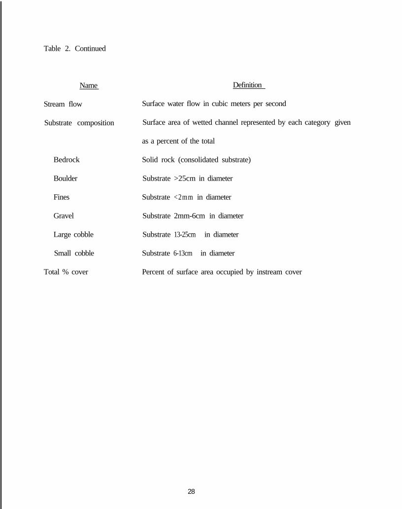
Table 2. Continued

Name

Stream flow

Substrate composition

Bedrock

Boulder

Fines

Gravel

Large cobble

Small cobble

Total % cover

Definition

Surface water flow in cubic meters per second

Surface area of wetted channel represented by each category given

as a percent of the total

Solid rock (consolidated substrate)

Substrate >25cm in diameter

Substrate <2mm in diameter

Substrate 2mm-6cm in diameter

Substrate 13-25cm in diameter

Substrate 6-13cm in diameter

Percent of surface area occupied by instream cover

28

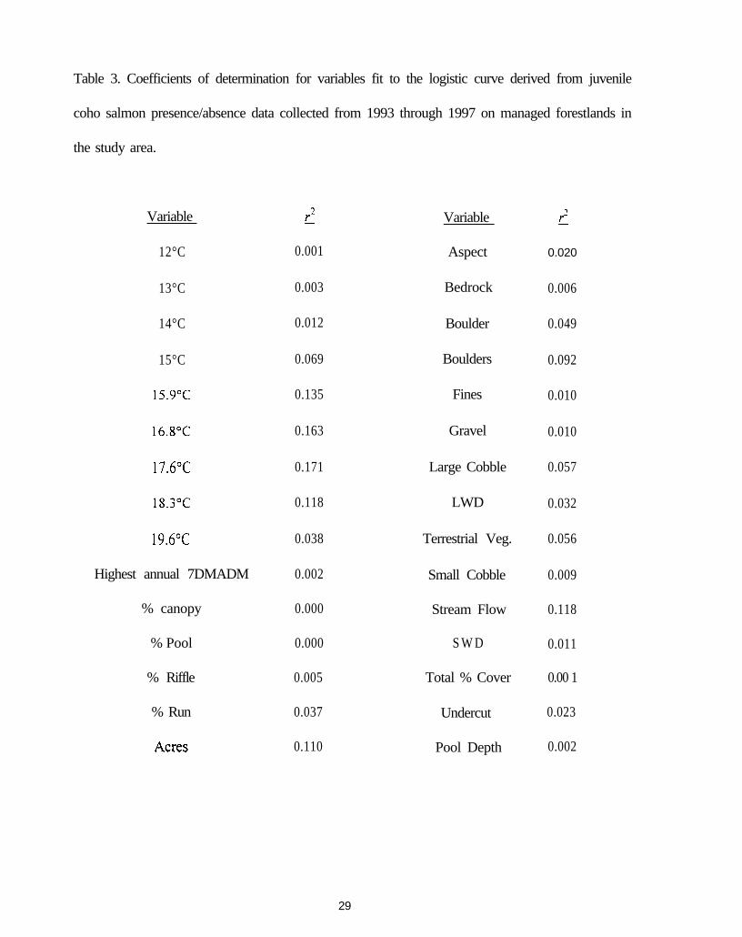
Table 3. Coefficients of determination for variables fit to the logistic curve derived from juvenile

coho salmon presence/absence data collected from 1993 through 1997 on managed forestlands in

the study area.

Variable

12°C

2r

0.001

13°C 0.003

Variable

Aspect

Bedrock

2.L

0.020

0.006

14°C 0.012 Boulder 0.049

15°C 0.069 Boulders 0.092

15.9”C 0.135 Fines 0.010

16.8”C 0.163 Gravel 0.010

17.6”C 0.171 0.057

18.3”C 0.118

Large Cobble

LWD 0.032

19.6”C

Highest annual 7DMADM

% canopy

% Pool

% Riffle

% Run

0.038 Terrestrial Veg.

Small Cobble

Stream Flow

S W D

Total % Cover

Undercut

Pool Depth

0.056

0.002

0.000

0.000

0.005

0.037

0.110

0.009

0.118

0.011

0.00 1

0.023

0.002

29

Table 4. Multivariate logistic regression models useful in describing the relationship of habitat variables to the presence and absence

of coho salmon within the study area. The X symbol indicates the variable in the respective row was included in the model. The AIC

score reflects the model’s performance. The model with the lowest score is best able to explain the presence and absence of juvenile

coho salmon. The log-likelihood is used for significance testing.

Variable

Days >15.9”CDays >16,8”CDays >17.6”CDays >18.3”C

H. A. 7DMADMBoulder (cover)

Boulders(substrate)

LWD (cover)Ter. veg. (cover)

Pool depthAIC score

I 2 1 4 5

XX

X XL

x x x xx x x x

x x x x

x x x x35.6 73.6 161.9 48.5 45.9

Model #

6 2 s 2 10

x x xX

Xx x x Xx x x x

x x x x xX x x

x x x x x49.0 54.5 36.2 38.8 37.3

II

X

XX

XX

38.0

X

XX

XX

48. I

13 14

x x

X

XX

x x

38.6 81.7Log-likelihood -11.79 -31.79 -78.93 -18.27 -16.93 -18.51 -21.23 -11.12 -12.41 -12.65 -12.99 -18.03 -15.27 -35.85

30