Evaluation of seepage problem under a concrete dam …€¦ · · 2009-09-08Evaluation of seepage...
7
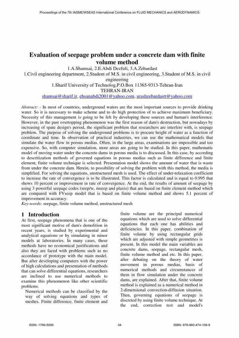
Evaluation of seepage problem under a concrete dam with finite volume method 1.A.Shamsai, 2.E.Abdi Dezfuli, 3.A.Zebardast 1.Civil engineering department, 2.Student of M.S. in civil engineering, 3.Student of M.S. in civil engineering 1.Sharif University of Technolog,P.O.Box 11365-9313-Tehran-Iran TEHRAN-IRAN [email protected] , [email protected] , [email protected] Abstract: - In most of countries, underground waters are the most important sources to provide drinking water. So it is necessary to make scheme and to do high protection of to achieve maximum beneficiary. Necessity of this management is going to be felt by developing these sources and human's interference. However, in the past overtopping phenomenon was the first reason of dam's destruction, but nowadays by increasing of spate design's period, the significant problem that researchers are interfere with, is seepage problem. The purpose of solving the underground problems is to procure height of water as a function of coordinate and time. In observation of practical industries, we can use the mathematical models that simulate the water flow in porous medias. Often, in the large areas, examinations are impossible and too expensive. So, with computer simulation, more areas are going to be studied. In this paper, mathematic model of moving water under the concrete dams in porous media is to discussed. In this case, by according to descritization methods of governed equations in porous medias such as finite difference and finite element, finite volume technique is selected. Presentation model shows the amount of water that is waste from under the concrete dam. Herein, to possibility of solving the problem with this method, the media is simplified. For solving the equations, unstructured mesh is used. The effect of under-relaxation coefficient to increase the rate of convergence is to be illustrated. This factor is calculated and is equal to 0.995 that shows 10 percent or improvement in rate of convergence. At the end, the results of amount of seepage by using 3 powerful seepage codes (seep/w, mseep and plaxis) that are based on finite element method which are compared with FVseep model that is based on finite volume method and shows 5.1 percent of improvement in accuracy. Key-words: seepage, finite volume method, unstructured mesh 1 Introduction At first, seepage phenomena that is one of the most significant motive of dam's demolition in recent years, is studied by experimental and analytical equations or by simulating in minor models at laboratories. In many cases, these methods have no economical justifications and also they are faced with problems such as no accordance of prototype with the main model. But after developing computers with the power of high calculations and presentation of methods that can solve differential equations, researchers are inclined to use numerical methods to examine this phenomenon like other scientific problems. Numerical methods can be classified by the way of solving equations and types of meshes. Finite difference, finite element and finite volume are the principal numerical equations which are used to solve differential equations that each one has abilities and deficiencies. In this paper, combination of finite volume by using rectangular grids which are adjusted with simple geometries is present. In this model the main variables are concrete dams, seepage, rectangular mesh, finite volume method and etc. In this paper, after debating on the theory of water movement in porous medias, basis of numerical methods and circumstances of them in flow simulation under the concrete dams, are explained. After that, finite volume method is explained as a numerical method in 2-dimensional convection-diffusion situation. Then, governing equations of seepage is discreted by using finite volume technique. At the end, correction test and model's Proceedings of the 7th IASME/WSEAS International Conference on FLUID MECHANICS and AERODYNAMICS ISSN: 1790-5095 34 ISBN: 978-960-474-106-9
Transcript of Evaluation of seepage problem under a concrete dam …€¦ · · 2009-09-08Evaluation of seepage...
Evaluation of seepage problem under a concrete dam with finite
volume method 1.A.Shamsai, 2.E.Abdi Dezfuli, 3.A.Zebardast
1.Civil engineering department, 2.Student of M.S. in civil engineering, 3.Student of M.S. in civil
engineering
1.Sharif University of Technolog,P.O.Box 11365-9313-Tehran-Iran
TEHRAN-IRAN
[email protected], [email protected], [email protected]
Abstract: - In most of countries, underground waters are the most important sources to provide drinking
water. So it is necessary to make scheme and to do high protection of to achieve maximum beneficiary.
Necessity of this management is going to be felt by developing these sources and human's interference.
However, in the past overtopping phenomenon was the first reason of dam's destruction, but nowadays by
increasing of spate design's period, the significant problem that researchers are interfere with, is seepage
problem. The purpose of solving the underground problems is to procure height of water as a function of
coordinate and time. In observation of practical industries, we can use the mathematical models that
simulate the water flow in porous medias. Often, in the large areas, examinations are impossible and too
expensive. So, with computer simulation, more areas are going to be studied. In this paper, mathematic
model of moving water under the concrete dams in porous media is to discussed. In this case, by according
to descritization methods of governed equations in porous medias such as finite difference and finite
element, finite volume technique is selected. Presentation model shows the amount of water that is waste
from under the concrete dam. Herein, to possibility of solving the problem with this method, the media is
simplified. For solving the equations, unstructured mesh is used. The effect of under-relaxation coefficient
to increase the rate of convergence is to be illustrated. This factor is calculated and is equal to 0.995 that
shows 10 percent or improvement in rate of convergence. At the end, the results of amount of seepage by
using 3 powerful seepage codes (seep/w, mseep and plaxis) that are based on finite element method which
are compared with FVseep model that is based on finite volume method and shows 5.1 percent of
improvement in accuracy.
Key-words: seepage, finite volume method, unstructured mesh
1 Introduction At first, seepage phenomena that is one of the
most significant motive of dam's demolition in
recent years, is studied by experimental and
analytical equations or by simulating in minor
models at laboratories. In many cases, these
methods have no economical justifications and
also they are faced with problems such as no
accordance of prototype with the main model.
But after developing computers with the power
of high calculations and presentation of methods
that can solve differential equations, researchers
are inclined to use numerical methods to
examine this phenomenon like other scientific
problems.
Numerical methods can be classified by the
way of solving equations and types of
meshes. Finite difference, finite element and
finite volume are the principal numerical
equations which are used to solve differential
equations that each one has abilities and
deficiencies. In this paper, combination of
finite volume by using rectangular grids
which are adjusted with simple geometries is
present. In this model the main variables are
concrete dams, seepage, rectangular mesh,
finite volume method and etc. In this paper,
after debating on the theory of water
movement in porous medias, basis of
numerical methods and circumstances of
them in flow simulation under the concrete
dams, are explained. After that, finite volume
method is explained as a numerical method in
2-dimensional convection-diffusion situation.
Then, governing equations of seepage is
discreted by using finite volume technique. At
the end, correction test and model's
Proceedings of the 7th IASME/WSEAS International Conference on FLUID MECHANICS and AERODYNAMICS
ISSN: 1790-5095 34 ISBN: 978-960-474-106-9

calibration is done by using 3 powerful
seepage codes (Mseep, Plaxis and Seep/w)
that are based on finite element method.
Scientists and researchers were interested in
seepage problems from the past. Henry Darcy
was one of the persons who tendered its basis
[1]. This phenomenon can be introduced by
Darci's Law and continuity equations.
Patankar has applied finite volume method to
evaluate heat transfer in 1972. Between 1978
and 1979, he has used finite volume method
to study the fluid mechanics and he got good
results. In 1980, he has used this procedure
with a high accuracy in fluid dynamics. This
method has a high flexibility even in
problems with unstructured meshes.
This system has been developed by White in
1986. At the same year, Anderson has done a
vast study on usage of this method to solve
differential equations and achieved valuable
results. In 1988, Wheiser used finite element
method to evaluate elliptic problems. At the
same time, Samon presented a new method that
is called quadratic convergence, to solve
differential equations and compare it with
classic methods and finally found out that this
method is adequate with finite volume
technique. In 1996, Baranger and his colleagues
studied corresponding between finite volume
method and finite element method and got
worth results. In 2003, Eymard used finite
volume method in solving Navier-Stokes
equations. At the same time, Angerman and his
assistants exhibited cell-centered style that
works with finite volume method and according
to achieved results we can assure that is a
idealist way to discrete differential equations. In
2004, Bertezolai investigated that finite volume
technique in solving convection diffusion
equations with non-structured grids. Finite
volume method analyzed by Domolo in 2005.
The advantage of finite volume method is to use
it in every grid and without any limitations.
2 Governing equations on seepage
in porous Medias: A public flow sources such as φ is
contemplated. By emphasizing on
conservation equations, the summation of φ
rate increasing by pure flow rate φ in one
element is equal to rate of increasing φ
because of diffusion and source. This
substance in mathematic is called convection
equation. We consider this equation in (1) as
below:
(1)
where, div ( ur
ρφ ) is the convection term and
( )φΓgrad is the diffusion term ( Γ is the
diffusion coefficient) [].
This equation is the first step on calculations
in finite volume method. If we integrate from
this equation in 3 dimensions, convection
equations will be gained.
(2)
By using Gauss Divergence Theory, we can
suppose that convection and diffusion term
can be explained as integral equations on
boundary condition surfaces:
(3)
In steady state problems, because of no
mutation toward time, we can compress
equation (3) and gain below equation:
(4)
In turbulent flows, we should integrate from
equation (2) between time t to t+ t∆ :
(5)
2.1. Finite volume method in diffusion: Diffusion equation can be obtained by
omitting the unsteady sources and convection
term:
(6)
0)( =+Γ φφ Sgraddiv
By integrating on equation (6), the final
equation has been prepared:
(7)
Now we can descrited the above equation in
2-D media.
2.2. Usage of finite volume method in 2-
D diffusion problems:
Governing equation on 2-D diffusion is
illustrated as equation (8):
( ) ( ) ( ) φφρφρφ
Sgarddivudivt
+Γ=+∂
∂ r
( ) ( ) ( ) ∀+∀Γ=∀+∀∂
∂∫∫∫∫
∀∀∀
dSdgraddivdudivdt
ccc
φφρφρφ r
( ) ( ) ∫∫∫∫∀
φ
∀
∀+φΓ=ρφ+∀ρφ∂
∂
cAAc
dSdAgrad.ndAu.ndt
r
( ) ( )∫ ∫ ∫∀
+Γ=A A C
dASdAgradndAun φφρφ ..r
( ) ( )∫ ∫∫∫∀∀∀
=∀+Γ=∀+∀ΓA CCC
dSdAgradndSdgraddiv 0. φφ φφ
0=+
∂
φ∂Γ
∂
∂+
∂
φ∂Γ
∂
∂S
yyxx
( ) ( )∫ ∫ ∫ ∫ ∫∫∫ ∫∆ ∆ ∆ ∀
φ
∆ ∀
∀+φΓ=ρφ+
∀ρφ
∂
∂
t A t t cAt c
dtdSdAdtgrad.ndAdtu.ndtdt
r
Proceedings of the 7th IASME/WSEAS International Conference on FLUID MECHANICS and AERODYNAMICS
ISSN: 1790-5095 35 ISBN: 978-960-474-106-9

un
PN
nnS
SP
SS
E
pE
ee
w
wp
WW
PP
pN
nn
PN
Ss
wp
Ee
wp
w
Sy
A
Y
A
x
A
x
A
Sy
A
Y
A
x
A
x
wA
+φ
∂
Γφ+
∂
Γφ
∂
Γ+φ
∂
Γ
=φ
−
∂
Γ+
∂
Γ+
∂
Γ+
∂
Γ
In figure (1) we can observe part of a 2-D grid
that is used for descriting equations.
Figure (1).2-D grids
In 2-D grids, in addition to points which are
situated on right (E) and left (W), two more
points denominated N and S are positioned on
up and down. Now, we can use the (8) equation
as (9):
(9)
According to yAA we ∆==
and xAA sn ∆== , equation (9) can be
corrected as follows:
(10)
0=∀∆+
∂
φ∂Γ−
∂
φ∂Γ+
∂
φ∂Γ−
∂
φ∂Γ s
yA
yA
xA
xA
s
ss
n
nn
w
ww
e
ee
As is mentioned before, this equation shows the
equilibrium of φ in a control volume.
Therefore, we can calculate the transmission
flow in a control volume as below equations:
Transmission flow from left
(11) ( )
wp
wp
ww
w
wwx
Ax
Aδ
φ−φΓ=
∂
φ∂Γ
Transmission flow from right
( )
pE
pe
ee
e
eex
Ax
Aδ
φφφ −Γ=
∂
∂Γ (12)
Transmission flow from top
(13)
Transmission flow from below
(14)
By substituting these equations in (10)
equation, we can have equation (15):
( ) ( ) ( ) ( )
0=∀∆+δ
φ−φΓ−
δ
φ−φΓ+
δ
φ−φΓ−
δ
φ−φΓ S
yA
yA
xA
xA
sp
SP
SS
PN
PN
nn
wp
WP
WW
PE
P
eeE
(15)
If we consider the source term as a linear
equation, equation (15) can be illustrated like
equation (16) as follows:
(16)
This equation is a final form of Laplace
equation and we should program our code in
Matlab software. This code is called
"FVseep" that contains sub-programs that
each one calculates particular things. These
sub-programs are managed by a main m-file
and after preparing unstructured meshes, flow
lines and potential lines and also the amount
of wasting water are calculated.
2.3. Presentation of FVseep Model: Fvseep model has a main routine and four
sub-routines. The main program is managed
sub-routines and controlled them. At first, by
calling sub-programs, Laplace equation has
solved in porous media. This program has got
some abilities like soil situation definition,
soil porosity and hydraulic conductivity in
two directions.
2.3.1. Structure of sub-routines: Sub-programs have below roles in FVseep
model:
- Geometry Definition
- Calculations of control volume
- Calculating governing equations
- Preparing graphical solutions
This model, divides the porous media by
rectangular meshes. In this case, we have 504
elements that intersect the media into smaller
pieces. An appropriate grid in numerical
methods is a grid that can increase the rate of
solutions in calculation's procedure and
causes the best accuracy with minimum
iterations. So, type and the geometry of grids
∫∫∫∀∆
φ
∀∆∀∆
=∂∀+∂∂
∂
φ∂Γ
∂
∂+∂∂
∂
φ∂Γ
∂
∂0Syx
yyyx
xx
( )
PN
PNnn
n
nny
Ay
Aδ
φ−φΓ=
∂
φ∂Γ
( )
sp
SPSS
S
Ssy
Ay
Aδ
φ−φΓ=
∂
φ∂Γ
unnssEEWWpp Saaaaa +φ+φ+φ+φ=φ
Proceedings of the 7th IASME/WSEAS International Conference on FLUID MECHANICS and AERODYNAMICS
ISSN: 1790-5095 36 ISBN: 978-960-474-106-9
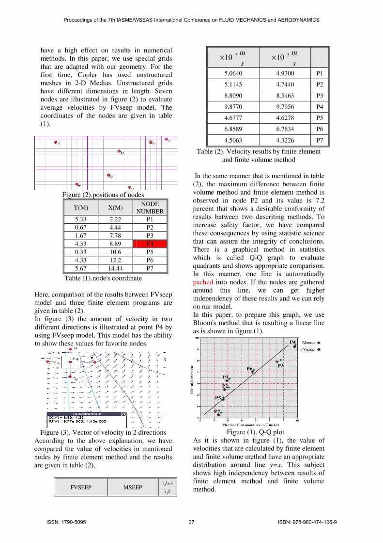
have a high effect on results in numerical
methods. In this paper, we use special grids
that are adapted with our geometry. For the
first time, Copler has used unstructured
meshes in 2-D Medias. Unstructured grids
have different dimensions in length. Seven
nodes are illustrated in figure (2) to evaluate
average velocities by FVseep model. The
coordinates of the nodes are given in table
(1).
Figure (2).positions of nodes
NODE
NUMBER X(M) Y(M)
P1 2.22 5.33
P2 4.44 0.67
P3 7.78 1.67
P4 8.89 4.33
P5 10.6 0.33
P6 12.2 4.33
P7 14.44 5.67
Table (1).node's coordinate
Here, comparison of the results between FVseep
model and three finite element programs are
given in table (2).
In figure (3) the amount of velocity in two
different directions is illustrated at point P4 by
using FVseep model. This model has the ability
to show these values for favorite nodes.
Figure (3). Vector of velocity in 2 directions
According to the above explanation, we have
compared the value of velocities in mentioned
nodes by finite element method and the results
are given in table (2).
شمارة
گرهMSEEPFVSEEP
s
m510−× s
m510−×
P1 4.9300 5.0640
P2 4.7440 5.1145
P3 8.5163 8.8090
P4 9.7956 9.8770
P5 4.6278 4.6777
P6 6.7634 6.8589
P7 4.3226 4.5063
Table (2). Velocity results by finite element
and finite volume method
In the same manner that is mentioned in table
(2), the maximum difference between finite
volume method and finite element method is
observed in node P2 and its value is 7.2
percent that shows a desirable conformity of
results between two descriting methods. To
increase safety factor, we have compared
these consequences by using statistic science
that can assure the integrity of conclusions.
There is a graphical method in statistics
which is called Q-Q graph to evaluate
quadrants and shows appropriate comparison.
In this manner, one line is automatically
pached into nodes. If the nodes are gathered
around this line, we can get higher
independency of these results and we can rely
on our model.
In this paper, to prepare this graph, we use
Bloom's method that is resulting a linear line
as is shown in figure (1).
Figure (1). Q-Q plot
As it is shown in figure (1), the value of
velocities that are calculated by finite element
and finite volume method have an appropriate
distribution around line y=x. This subject
shows high independency between results of
finite element method and finite volume
method.
Proceedings of the 7th IASME/WSEAS International Conference on FLUID MECHANICS and AERODYNAMICS
ISSN: 1790-5095 37 ISBN: 978-960-474-106-9

In figure (2), deviation of velocity values are
illustrated. As it is shown, similar nodes
approximately have the same distance from
normal line.
Figure(2).deviation from normal line
So, we can trust the results of FVseep model
with high safety factor. In continue, we
precisely analyzed the amount of seepage under
a small concrete dam by using 3 powerful
software that are based on finite element method
and then compared their results by FVseep
model.
Figure (4) shows geometry of this case study.
This figure shows a small concrete dam.
Potential head on upstream is 10 m and on
down stream is 1 m. hydraulic conductivity
coefficient in 2 directions is s
m410−. This area
is supposed to be porous media, rectangular and
has a 15 m in length and 6 m in height.
Figure (4).Geometry of porous media
The amount of error in all soft wares is 6105.0 −× and the maximum of iterations is
1000. In figure (5) are shown flow lines which
are solved by finite element method and finite
volume method.
Figure (5).finite element and volume flow
lines
As it is seen, they have approximately similar
graphical results. In table (3) velocity and
amount of discharge results are given. By
according to these values, difference between
the results is about 5.1 percent that is
appropriate with numerical methods.
Proceedings of the 7th IASME/WSEAS International Conference on FLUID MECHANICS and AERODYNAMICS
ISSN: 1790-5095 38 ISBN: 978-960-474-106-9
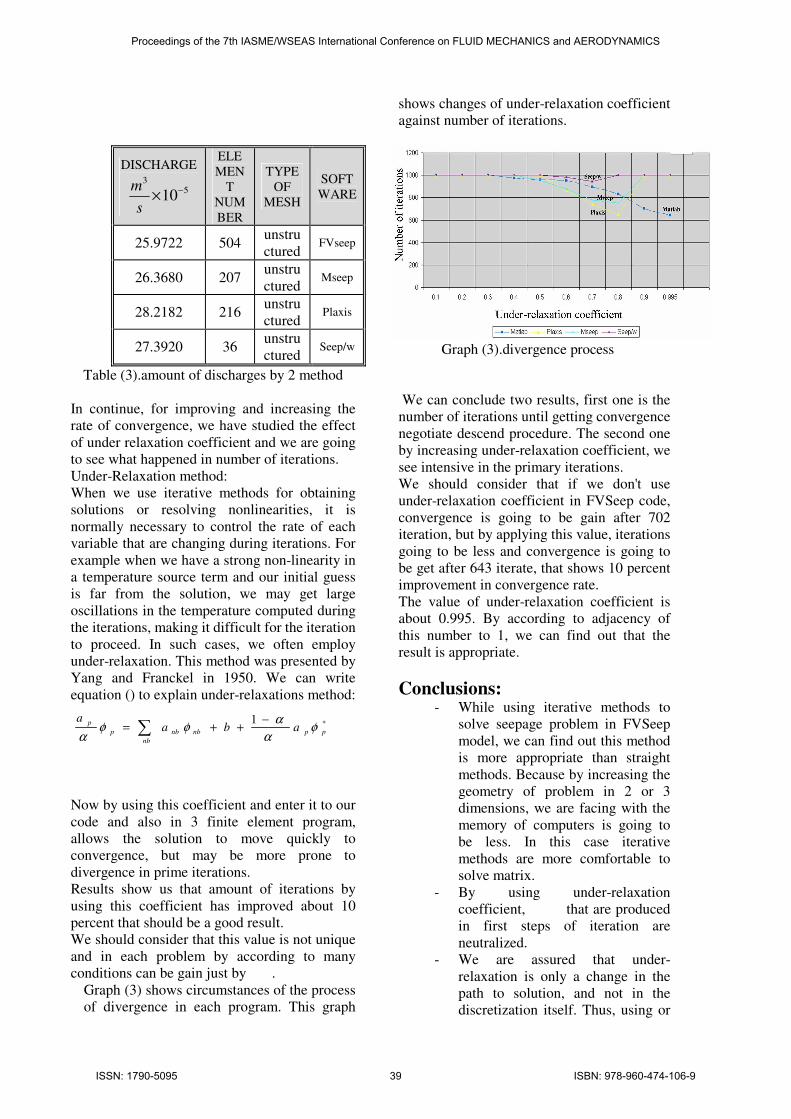
SOFT
WARE
TYPE
OF
MESH
ELE
MEN
T
NUM
BER
DISCHARGE
53
10−×s
m
FVseep unstru
ctured 504 25.9722
Mseep unstru
ctured 207 26.3680
Plaxis unstru
ctured 216 28.2182
Seep/w unstru
ctured 36 27.3920
Table (3).amount of discharges by 2 method
In continue, for improving and increasing the
rate of convergence, we have studied the effect
of under relaxation coefficient and we are going
to see what happened in number of iterations.
Under-Relaxation method:
When we use iterative methods for obtaining
solutions or resolving nonlinearities, it is
normally necessary to control the rate of each
variable that are changing during iterations. For
example when we have a strong non-linearity in
a temperature source term and our initial guess
is far from the solution, we may get large
oscillations in the temperature computed during
the iterations, making it difficult for the iteration
to proceed. In such cases, we often employ
under-relaxation. This method was presented by
Yang and Franckel in 1950. We can write
equation () to explain under-relaxations method:
Now by using this coefficient and enter it to our
code and also in 3 finite element program,
allows the solution to move quickly to
convergence, but may be more prone to
divergence in prime iterations.
Results show us that amount of iterations by
using this coefficient has improved about 10
percent that should be a good result.
We should consider that this value is not unique
and in each problem by according to many
conditions can be gain just by .
Graph (3) shows circumstances of the process
of divergence in each program. This graph
shows changes of under-relaxation coefficient
against number of iterations.
Graph (3).divergence process
We can conclude two results, first one is the
number of iterations until getting convergence
negotiate descend procedure. The second one
by increasing under-relaxation coefficient, we
see intensive in the primary iterations.
We should consider that if we don't use
under-relaxation coefficient in FVSeep code,
convergence is going to be gain after 702
iteration, but by applying this value, iterations
going to be less and convergence is going to
be get after 643 iterate, that shows 10 percent
improvement in convergence rate.
The value of under-relaxation coefficient is
about 0.995. By according to adjacency of
this number to 1, we can find out that the
result is appropriate.
Conclusions: - While using iterative methods to
solve seepage problem in FVSeep
model, we can find out this method
is more appropriate than straight
methods. Because by increasing the
geometry of problem in 2 or 3
dimensions, we are facing with the
memory of computers is going to
be less. In this case iterative
methods are more comfortable to
solve matrix.
- By using under-relaxation
coefficient, that are produced
in first steps of iteration are
neutralized.
- We are assured that under-
relaxation is only a change in the
path to solution, and not in the
discretization itself. Thus, using or
∑−
++=nb
ppnbnbp
paba
a*1
φα
αφφ
α
Proceedings of the 7th IASME/WSEAS International Conference on FLUID MECHANICS and AERODYNAMICS
ISSN: 1790-5095 39 ISBN: 978-960-474-106-9

deny using of this method have no
effect in results and just rate of
convergence is going to increase.
- The optimum value of α depends
strongly on the nature of the system
of equations we are solving, on how
strong the non-linearities are, on
grid size and so on. A value close to
unity allows the solution to move
quickly towards convergence, but
may be more prone to divergence.
References:
[1] Darcy, H., Les fontaines de la ville de
Dijon, Dalmont, Paris, 1856.
[2] Patankar, S.V, Numerical heat transfer
and fluid flow, Hemisphere, Washington,
D.C. .,1980.
[3] Manteufel, T. & White, A. The
numerical solution of second-order
boundary value problems on nonuniform
meshes. Math. Comput., 47, pp:511-535.,
1986.
[4] Weiser, A. & Wheeler, M. On
convergence of block-centered finite
difference for elliptic problems. SIAM J.
Numer. Anal., 25, pp:351-375,. 1988.
[5] Forsyth, P. & Sammon,P. Quadratic
convergence for cell-centered grids. Appl.
Numer: Math., 4, pp:377-394,. 1988.
[6] Baranger, J., Maitre, J. F. & Oudin, F.
Connection between finite volume and
mixed finite element methods, Math, Mod.
Numer: Anal., 30, pp:445-465,. 1996.
[31] Eymard,R., Gallouet, T. & Herbin, R.
Finite volume methods, Handbook of
Numerical Analysis, vol. 7 (P.Ciarlet & J.-
L. Lions, eds). Amesterdam: North Holland,
pp:723-1020,. 2000.
[7] Eymard, T. & Herbin, R. Afinite volume
scheme on general meshes for the steady
Navier-Stokes problem in two space
dimensions. Technical report, LAPT, Aix-
Marseille 1,. 2003.
[8] Angermann, L. Node-centered finite
volume schemes and primal-dual mixed
formulations. Commun Appl. Anal., 7,
pp:529-566,. 2003.
[9] Bertolazzi, E. & Manzini, G. A cell-
centered second-order accurate finite
volume method for convection-diffusion
problems on unstructured meshes. Math.
Models Methods Appl.Sci., 14, pp:1235-
1260,. 2004.
[10] Domelevo, K. & Omnes, P. Afinite
volume method for the Laplace equation o
almost arbitrary two-dimensional grids.
ESAIM: Math. Model. And Num. Anal. (to
appear),. 2005.
[11] Droniou, J. & Eymard, R. A mixed
finite volume scheme for anisotropic
diffusion problems on any grid. Preprint
available at http://hal.ccsd.cnrs.fr/ccsd-
00005565 (submitted),.2005.
Proceedings of the 7th IASME/WSEAS International Conference on FLUID MECHANICS and AERODYNAMICS
ISSN: 1790-5095 40 ISBN: 978-960-474-106-9