Evaluation of policies for water quality improvement in ...

1

Evaluation of policies for water quality improvement

in the Upper Waikato catchment

Graeme J. Doole1

1 Department of Economics, Waikato Management School, University of Waikato, Private

Bag 3105, Hamilton, New Zealand.

2

1. Introduction

The National Policy Statement (NPS) for Freshwater Management 2011 provides the

foundation for regional councils in New Zealand to set the appropriate objectives and targets

for freshwater quality. The National Objectives Framework (NOF) provides guidance to

regional bodies for this activity, while also providing some national integration. The NOF

primarily provides an extensive list of potential values—such as electricity generation,

swimming, and irrigation—that regions can determine as appropriate activities to safeguard

from water quality decline. Two values are compulsory across all regions: (1) ecosystem

health and general protection for indigenous species, and (2) safety for secondary human

contact. Each value has a set of related attributes of water quality; for example, irrigation

requires that Escherichia coli, flows, and sediment levels are appropriately managed. The

NOF provides specific water quality targets—organised into A, B, C, and D bands—

associated with each attribute. The D level is not an appropriate goal, but rather represents

deterioration beyond an acceptable standard. Each region can select which values are

important to safeguard and to what degree these should be satisfied, on a case-by-case basis.

By design, policies to improve the quality of freshwater resources have strong potential to

impact current and future management through manipulating the set of incentives that various

stakeholders face. Achieving water quality improvement in many New Zealand catchments

will likely require significant manipulation of existing land management, given the intensive

nature of New Zealand’s agricultural industries and that point sources have been now been

well regulated in most places. The New Zealand Government seeks to support regional

bodies in managing water quality. Accordingly, the Ministry for the Environment, DairyNZ,

Waikato River Authority, and Waikato Regional Council have recently combined within the

Waikato Joint Venture Project (WJVP) to provide robust input into water quality outcomes in

the Waikato River catchment.

The primary objective of this study, as a project funded by the WJVP, is to assess the

economic impact of various policies to improve water quality outcomes in the Upper Waikato

catchment. Economic modelling provides an important means to assess the cost and

distributional implications of alternative policies associated with improved water quality

(Doole, 2012). Accordingly, a flexible framework for land-use optimisation within the

context of various policy options is developed and applied.

3

The report is structured as follows. Section 2 provides a concise description of the model and

summarises the policy scenarios. Section 3 presents results and discussion, while Section 4

summarises the key findings of this research.

2. Methods

2.1 The Land Allocation and Management (LAM) model

The applied framework—the Land Allocation and Management (LAM) model—integrates

information from a variety of sources to provide steady-state predictions of the possible

impacts of agri-environmental policy (Doole et al., 2013). Variants of this framework have

been applied throughout New Zealand (Howard et al., 2013) and Australia (Doole et al.,

2013). The LAM model is a nonlinear optimisation model (Bazaraa et al., 2006) that

identifies the land-use pattern and the management within each land use that maximises

profit. Different policy instruments may be simulated through setting constraints on relevant

decision variables within the model. For example, the NPS scenarios in the following

application involve median nitrate and chlorophyll-A concentrations not going above their

current level. This is simulated through setting constraints on these quantities.

This section describes the LAM model and how different policy scenarios are simulated. The

model is based on two important concepts. A land use describes the type of enterprise that

exists on that parcel of land (e.g. dairy, forestry). A management option for a given land use

represents a specific type of management within that land use.

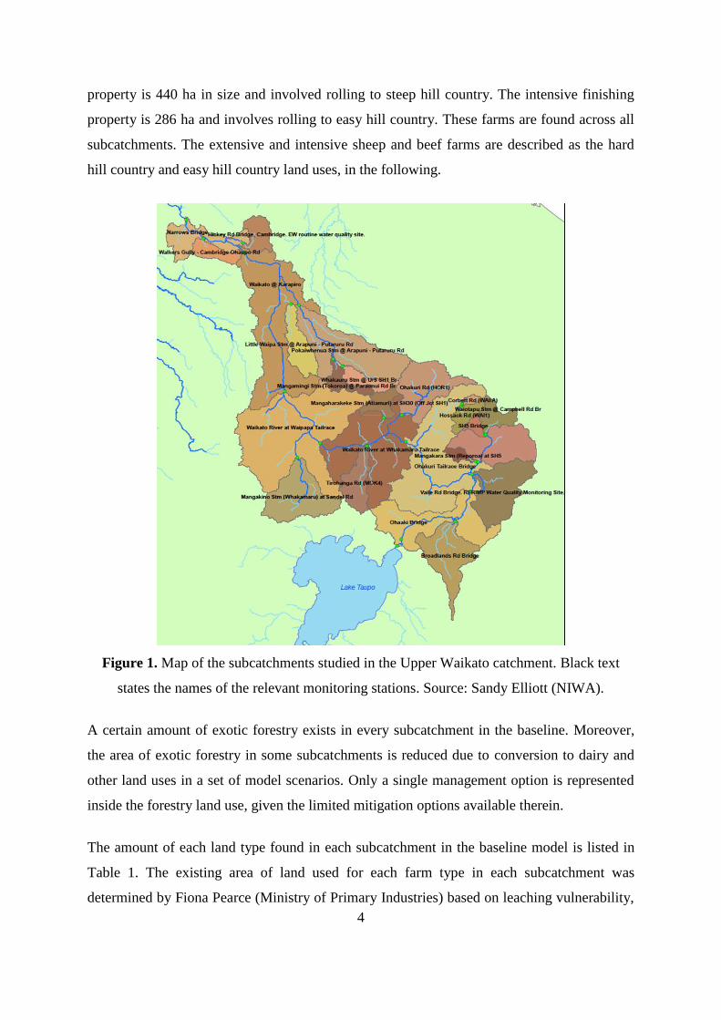
The Upper Waikato catchment represented in this study consists of 24 subcatchments (Figure

1) that have been formulated based on their common hydrological attributes and placement

relative to Waikato Regional Council water monitoring stations. Each one of these

subcatchments is associated with a given monitoring station at its terminal point. The

economic model is thus defined over a set of 24 subcatchments.

DairyNZ divided the dairy farming systems found across the catchment into 14 representative

types or clusters, which are scattered across 23 of the 24 subcatchments in the absence of

dairy conversion and all of the subcatchments in the presence of dairy conversion. AgFirst

divided the sheep and beef farming systems found across the catchment into 2 representative

types: an extensive hill property, and an intensive finishing property. The extensive hill

4

property is 440 ha in size and involved rolling to steep hill country. The intensive finishing

property is 286 ha and involves rolling to easy hill country. These farms are found across all

subcatchments. The extensive and intensive sheep and beef farms are described as the hard

hill country and easy hill country land uses, in the following.

Figure 1. Map of the subcatchments studied in the Upper Waikato catchment. Black text

states the names of the relevant monitoring stations. Source: Sandy Elliott (NIWA).

A certain amount of exotic forestry exists in every subcatchment in the baseline. Moreover,

the area of exotic forestry in some subcatchments is reduced due to conversion to dairy and

other land uses in a set of model scenarios. Only a single management option is represented

inside the forestry land use, given the limited mitigation options available therein.

The amount of each land type found in each subcatchment in the baseline model is listed in

Table 1. The existing area of land used for each farm type in each subcatchment was

determined by Fiona Pearce (Ministry of Primary Industries) based on leaching vulnerability,

5

slope, and current land use information. Leaching vulnerability is used to classify different

dairy farms, according to their respective impact of on water quality outcomes. However, it is

recognised that this is not currently used by most, if not all, dairy farmers when making land

use decisions. Urban and miscellaneous land uses do not change across scenarios and have a

fixed leaching load associated with them.

Table 1. Areas of each subcatchment in the Upper Waikato catchment model.

Subcatchment

name

Dairy

area

Suppor

t area

Easy

hill

Hard

hill

Exotic

forest

Urba

n

Misc. Total

Pueto 0 0 1,881 36 16,728 56 1,327 20,029

Waikato at

Ohaaki 2,792 572 9,247 611 8,130 699 6,958 29,009

Torepatutahi 7,342 1,504 898 62 11,126 54 736 21,721

Waiotapu at

Campbell 378 77 1,566 370 2,955 2 731 6,079

Kawaunui 1,103 226 233 147 214 0 211 2,134

Mangakara 387 79 890 412 42 0 425 2,235

Waiotapu at

Homestead 6,134 1,256 417 34 10,247 13 2,376 20,478

Whirinaki 136 28 557 340 0 0 19 1,080

Otamakokore 2,113 433 831 222 81 21 871 4,573

Waikato at

Ohakuri 12,972 2,657

17,00

5 5,392 8,306 26 6,781 53,139

Tahunaatara 4,682 959 4,163 863 5,153 0 4,996 20,816

Mangaharakek

e 823 169 179 14 4,230 0 0 5,415

Waipapa

Stream 2,965 607 2,789 127 885 2 2,674 10,049

Waikato at

Whakamaru 7,362 1,508 4,524 1,358 24,116 36 5,762 44,665

Mangakino 4,795 982 6,340 704 1,252 0 8,112 22,186

Waikato at

Waipapa 9,271 1,899 8,233 1,496 28,662 351

19,48

0 69,392

Whakauru Stm 1,329 272 1,267 32 1,720 146 537 5,302

Mangamingi 2,024 415 280 52 1,137 679 589 5,175

Pokaiwhenua 10,684 2,188 1,579 92 14,418 28 3,713 32,701

Little Waipa 6,678 1,368 1,094 66 807 0 637 10,649

Waikato at

Karapiro 21,216 4,346 8,907 2,000 5,680 195

11,62

4 53,969

Karapiro

Stream 1,989 407 2,629 614 66 0 1,036 6,741

Mangawhero 2,778 569 463 157 11 33 1,337 5,347

Waikato at

Narrows 5,048 1,034 394 165 79 895 5,372 12,987

Totals 115,00 23,555 76,36 15,36 146,04 3,236 86,30 465,871

6

1 6 6 5 4

The proportion of each land use in the Upper Waikato catchment is represented in Figure 2.

Land use within each of the farm types is allocated between a range of management options.

For example, if 200 ha is allocated to dairy farming in a given subcatchment, then this will be

split between a set of management options (e.g. 150 ha to standard production and 50 ha with

standard production and a stand-off pad). Each of the 14 dairy farm types have 7 basic

management options that represent a range of farming systems. These management options

differ markedly, but are designed so that leaching rates range from the baseline level to 50%

of the baseline level. This diversity allows the analysis of broad changes in dairy farm

management under a given policy. These 7 management options are replicated across 3

different situations: (1) spray effluent from the sump, (2) spray effluent from a holding pond,

and (3) use a stand-off pad and spray effluent from a holding pond. Thus, there is a total of 21

dairy farm management options within each of the 14 farm types. The production,

management, and leaching loads associated with each management option are determined

using DairyNZ information, nutrient modelling using OVERSEER (Wheeler et al., 2006),

and optimisation modelling using GSL (Ridler et al., 2001).

Figure 2. The proportion of each land use in the Upper Waikato catchment.

There are 28 management options for each of the hard hill country and easy hill country land

uses. The production, management, and leaching loads associated with each option are

25%

5%

16%

3%

31%

1%

19%

Dairy

Support

Easy hill

Hard hill

Forest

Urban

Misc.

7

determined by AgFirst using FARMAX, discounted cash flow modelling, and OVERSEER

modelling. Forestry options generated by AgFirst are not considered since Scion information

provides more accurate values for the value of forestry management in each subcatchment.

Also, 2m riparian strips considered in the AgFirst data are not replicated in the model since

Waikato Regional Council has confirmed that these are not generally considered of

appropriate effectiveness in the study region to be incorporated. However, 4m and 6m

riparian strips considered in the AgFirst data are incorporated.

The catchment model identifies the decision variables that maximise the total operating

surplus, subject to the constraints defined in the model. It is appropriate to study operating

surplus in the model, as a lack of information prevents an accurate depiction of how tax,

depreciation, drawings, and interest payments affect returns on all land uses

(especially forestry and sheep and beef land). The primary decision variables in the

model are those representing the area (ha) allocated to each management option within

each land use. The total operating surplus is determined through multiplication of the

area of each land use option employed and its associated level of operating surplus per

ha. The total nitrogen load for each subcatchment is computed through the multiplication

of the area of each land use option employed and the nitrogen leaching load per ha

associated with each management option. The total phosphorus load for each subcatchment

is computed through the multiplication of the area of each land use option employed and the

phosphorus leaching load per ha associated with each option.

The nutrient loads for each subcatchment are subject to attenuation (nutrient losses

between their source and subsequent monitoring stations), described through a

hydrological model (Elliott and Semadeni-Davies 2013) that has been replicated in the

economic model. The incorporation of these factors allows the nutrient load arising from

each subcatchment reaching the monitoring station within another subcatchment to be

explicitly defined. The loads present at each monitoring station are used as inputs to

calculate median total nitrate, total N (TN), and total P (TP) concentrations at each

station, for catchment equilibrium conditions.

The hydrological model is described further in Elliott and Semadeni-Davies (2013), but

is summarised briefly here.

8

The catchment is broken into 24 subcatchments, based on the location of water quality

monitoring stations. For each subcatchment, the mean annual load of nutrients generated

within the catchment is determined based on a) pasture losses, as provided by the

economic model; b) exotic forest, urban, and other diffuse losses (e.g. scrub),

determined from land areas multiplied by yield coefficients; c) point sources, derived

from discharge records; and d) geothermal inputs of nitrogen, derived from analysis of

stream water quality.

The diffuse sources are subject to attenuation before entry into the main stem of the river

network. The subcatchment-average attenuation factors for phosphorus are taken from

the CLUES catchment model and then modified to improve the match to measured mean

annual loads for TP. For TN, the situation is more complicated, and it is inappropriate to

calibrate solely to measured loads, because the current measured TN load may

underestimate the equilibrium situation, due to groundwater lags. An approach is

adopted whereby three different levels of attenuation are analysed, bracketing the expected

range. The largest attenuation is estimated by calibrating to match current measured mean

annual loads exactly; this will over-estimate the attenuation in many cases, because the

current load at calibration sites will be lower than the steady-state value. Some judicious

lumping of decay coefficients between adjactent subcatchments is required to avoid

unreasonable decay coefficients (such as negative attenuation). The resulting loss

percentages ranged from 0 to 75%, with a median of 45%. The low attenuation scenario

applied an estimated lower bound of the attenuation coefficient, generally a loss of 20%,

except where the ‘maximum’ attenuation as described above was already less than this

value. This approach will tend to be conservative, in the sense that it will tend to

provide higher load estimates. An intermediate attenuation scenario is also applied, in

which the attenuation was between the maximum and minimum values, and typically

represented a 30% loss.

Attenuation within the main-stem (including the hydro reservoirs) is also applied. This

attenuation, which is generally only a few percent, is taken from the CLUES catchment

model (which uses an effective settling velocity), with an adjustment in some cases for TN

to ensure that the within-catchment attenuation is within reasonable bounds.

9

The resulting load at a monitoring station is then determined as the sum of the loads from

upstream, discounted for within-subcatchment and mainstem attenuation.

The mean annual concentrations are then determined from load in the following way. For

TP, the proportional change in load under a scenario is applied to the current measured TP

concentration to derive the predicted concentration for the scenario. For example, if the

loads increased by 10% at a monitoring station, then the concentration increases by 10%

from the current mean value. For TN, a similar approach is adopted, except that the

proportional increase in load is determined with reference to the current concentration as

estimated from the low-attenuation scenario (which matches current measured loads, where

available).

The TN and TP concentrations are each related to chlorophyll-A concentration at 5 sites

along the Waikato River: Ohaaki, Ohakuri, Whakamaru, Waipapa, and the Narrows. The

relationship between nutrients and chorophyll is derived from regression relationships going

down the stream network, with an adjustment to ensure that the predicted value at a

particular station matches the current measured value. The hydrological model provided by

NIWA computes two quantities of chlorophyll-A: one quantity of chlorophyll-A

determined as a function of N, and one quantity of chlorophyll-A determined as a function

of P. Constraints placed on chlorophyll-A in the simulations require both quantities to be

less than the relevant threshold. This is necessary because the joint distribution of

chlorophyll-A as a function of both N and P is unknown and could not be determined from

the available data. However, this implies that neither of these nutrients is specifically

limiting chlorophyll-A populations in this waterway. Any interpretation of model output

must account for this limitation, given that a management focus on one nutrient, relative to

less attention paid to another, may be warranted if one is specifically limiting.

Land use allocation is governed by a series of model constraints. The total land allocated

between the management options in a given land use is constrained by the maximum area

covered by that land use in each subcatchment (Table 1). Each dairy management option

requires a given number of rising 1-year old, rising 2-year old, and mature cows to be grazed

off farm for a proportion of the year. The total number of each type of cow that requires

grazing off for a given set of management options is computed. Equations are then defined to

ensure that each cow type can be supported, under an assumption that 10% of cows are

10

grazed outside of the catchment (Ross Abercrombie, pers. comm.). Cows can be grazed on

the dedicated area of the catchment that consists of support blocks for dairy farms or on the

easy hill country (Table 1).

A high proportion of dairy farmers currently use holding ponds for effluent treatment.

(Survey information from DairyNZ highlights that this proportion is around 72% in the

catchment.) The proportion of farmers in each dairy farm type in each subcatchment with a

holding pond is drawn from DairyNZ survey information. A constraint for each subcatchment

is then defined to set a lower bound for the use of holding ponds. Holding ponds are more

expensive than spraying from the sump; thus, this constraint is met with equality in the

optimal solution. However, the proportion of farms with a holding pond supersedes this

baseline level when greater mitigation using this strategy is cost-effective.

The dynamics of land use change are difficult to describe in a land use optimisation model.

However, some land use change is permitted in this model to ensure that simulated targets are

feasible. By allowing this to happen, it is demonstrated how extreme remediation activity has

to be to achieve certain goals. There are several ways that land use can change away from its

baseline in the model. First, sheep and beef operations in the hard hill area can change their

sheep:beef ratio. Second, sheep and beef operations in the easy hill area can change their

sheep:beef ratio, fatten bulls, or graze dairy cows. Third, sheep and beef operations on the

easy and hard hill areas can be planted to exotic forest. Last, dairy and support land can be

planted to exotic forest or be used for sheep and beef farming. Simulating the afforestation of

agricultural land is controversial, but is undertaken in this study, given that NPS standards

cannot be met under the existing land allocation. While land use change is possible in the

model, it is only employed if on-farm mitigation practices within a given land use are

relatively unprofitable.

The model is solved using nonlinear programming with the CONOPT4 solver in the General

Algebraic Modelling System (GAMS) (Brooke et al., 2012). The catchment model contains

around 3,000 equations and around 18,000 decision variables.

11

2.2 Annual returns for dairy farms

Annual returns are computed with more detail for dairy farms, relative to the sheep and beef

farms incorporated in the catchment model, because of the detailed information provided by

the WJVP partner, DairyNZ. The method used and its description here follows Howard et al.

(2013).

Each dairy farm type contains a given number of farms in the baseline; these are considered

as individual enterprises in the model. We do not consider sharemilkers receiving only a

proportion of farm revenue. This is consistent with the available data and sharpens the focus

on the impact of alternative N leaching goals on farm profitability and viability.

Annual returns per ha for a single dairy farm are computed as: returns = surplus + dividend –

tax – depreciation – drawings – interest. Annual returns are computed with drawings (denoted

WD) and without drawings (denoted WOD) included, to demonstrate the impact of their

inclusion on annual returns. Farm operating surplus for a given farm type is mean operating

surplus per ha for that type. This is determined within the objective function of the model for

each farm type. Dividend is calculated through computation of mean milk production per ha

for that cluster. The assumption that a dividend of $0.35 per kilogram of milk solids is paid is

provided by DairyNZ. It is assumed that all farms in the catchment receive a dividend. This is

necessary since the number of suppliers to competing processing companies is unknown and

we do not know how the DairyBase data used to estimate debt level (see below) is impacted

by money borrowed to finance share purchases.

Tax is only borne if taxable income is positive. Taxable income is profit per ha after interest

payments and depreciation, but before drawings, have been accounted for. The tax rate is set

at $0.28 per dollar of taxable income based on the New Zealand company tax rate. Asset

depreciation is determined as a function of milk production. The $0.31 per kg MS assumption

for depreciation is taken from 2011/12 DairyBase data collected from 125 owner-operators in

the Waikato region. Drawings are calculated using the 2012 DairyBase labour adjustment for

management to represent the cost of owner-operator labour. This is determined as a function

of the number of cows on a given farm.

12

Annual interest costs are computed through multiplication of the interest rate and the total

debt level measured through closing term liabilities. (Liabilities and interest costs are

therefore underestimated due to the exclusion of current liabilities.) Annual interest costs (r)

are assumed to be 7 per cent of closing term liabilities (McCall, 2012). Closing term

liabilities per ha are taken from 2011/12 DairyBase data collected from 125 owner-operators

in the Waikato region. A cumulative distribution function for closing term liabilities is

estimated from this data using a kernel density estimator implemented in MATLAB (Miranda

and Fackler, 2002). Kernel density estimation is a non-parametric statistical estimation

technique that overcomes the need to make strong assumptions regarding the distribution of

the probability density function associated with a given data set (Greene, 2012). This function

is then used to generate a cumulative distribution function for each cluster for closing term

liabilities.

Land use change has no effect on the proportion of farmers who can cover costs in the model.

Given a lack of suitable resources, there is no link represented between these processes in the

model. Thus, the costs of land use change are not transferred to other land uses. The only

costs faced by dairy farmers are those imposed on dairy land that remains in dairy production.

As abatement costs are borne, this increases costs and hence decreases the proportion able to

cover costs.

A limitation of the approach described in this section is that debt levels are not related to

other farm factors, such as production and profitability. Thus, low-producing farms may end

up with higher debt levels that could be observed in reality. However, based on the same

arguments, high-producing farms may end up with lower debt levels also. The extent to

which effect is dominant is unknown.

2.3 Model runs

A number of different scenarios are simulated. These are listed in Table 2. Scenarios 1–3 are

the baseline solutions for the model, representing the current situation under different

assumptions regarding attenuation. This is justified since all subcatchments currently meet

the NOF standards, no trading takes place under current management, and no dairy

conversion is simulated within these runs.

13

Three different goals are simulated. Some relate to the historic medians of nitrate and

chlorophyll-A concentrations. The historic median for nitrate is the 20-year corrected median

(Sandy Elliott, pers. comm.). The historic median for chlorophyll-A is the 5-year uncorrected

median (Sandy Elliott, pers. comm.). The NOF goal requires that chlorophyll-A targets to

attain the Level C grade (less than 0.012 g/m3) are met at the Ohaaki, Ohakuri, Whakauru,

Waipapa, and Narrows stations on the Waikato River. Moreover, nitrate levels must achieve

at least a Level C grade (less than 6.9 g/m3) at all stations. Thus, nitrate and chlorophyll-A

levels may get worse than their current point, provided they do not reach the C grade. NOF

standards for TN and TP are not focused on specifically, as the chlorophyll-A target accounts

for these, at least to some extent, through its explicit relationship with these nutrient levels.

The NPS-av (NPS-average) standards are defined through requiring that the average

chlorophyll-A level across the Ohaaki, Ohakuri, Whakauru, Waipapa, and Narrows stations

on the Waikato River is maintained or improved. Additionally, the average nitrate level

across all relevant sites must be maintained or improved. This scenario is consistent with the

overall maintenance or improvement of water quality standards across the catchment,

allowing water quality in some specific subcatchments to degrade relative to the current

baseline and improve at others, provided the overall average is maintained or improved. The

NPS-all standards are defined through requiring that the chlorophyll-A levels at the Ohaaki,

Ohakuri, Whakauru, Waipapa, and Narrows stations on the Waikato River are maintained at

or below their historic medians. Additionally, nitrate levels must not surpass their historic

medians at all stations. The stringency of these simulated environmental standards increases

as we move rightwards across the list of: NOF – NPS-av – NPS-all.

Three assumptions regarding attenuation are simulated. An optimistic (high attenuation)

(HAT) scenario is simulated, in which high attenuation rates are used that are consistent with

existing increasing trends of N in the Upper Waikato catchment levelling off at the present

level from the current period onwards. A pessimistic (low attenuation) (LAT) scenario is also

simulated, in which low attenuation rates are used that are consistent with current increasing

trends of N in the Upper Waikato catchment continuing at their present rate to the point

where the concentrations reach a limit based on loading and with a small amount of

attenuation. A third scenario, a low-moderate attenuation (LMAT) rate, is also simulated for

illustrative purposes. It should be noted that there is considerable uncertainty around

14

estimates of attenuation. The HAT, LMAT, and LAT scenarios are consistent with average

losses across the catchment of 50%, 30%, and 20% between source and measurement.

The high attenuation scenario is consistent with short lag times between N loss and its

expression in waterways, and thus infers that there is a minor N load to come. In contrast, the

low attenuation scenarios are consistent with long lag times between N loss and their

expression in waterways, and thus infer that there is a significant N load arising from past

agricultural production yet to arrive.

The presence of different assumptions regarding attenuation rate alter the relationship

between the extent of mitigation activities and their impact on water quality outcomes. This

obviously has broad implications for the adoption of such activities and the associated

abatement cost. The concentration of chlorophyll-A is determined based on fixed

relationships that determine a level based on either TN and TP concentration, which are

computed from post-attenuated loads of N and P, respectively. However, within the results of

the economic modelling, the chlorophyll-A concentrations vary greatly across the different

scenarios (Table 9), in response to variation in TN and TP. This arises directly from the fact

that optimal levels of TN and TP change within each scenario, as alternative attenuation

assumptions are simulated.

Two scenarios are simulated for forestry conversion. First, a baseline case with no conversion

is simulated. This is based on the fact that water in the catchment is at, or close to being fully

allocated, constraining conversion. Second, the Waikato Regional Council, the Ministry for

the Environment, the Waikato River Authority, and DairyNZ have provided a scenario

whereby 25,000 ha is converted from exotic forestry to dairy production. This is based on the

assumption that some allocated water is not currently utilised, and/or that trading of water

may enable some conversions to take place. The subcatchments in which the hypothetical

conversions could potentially take place are unknown. For the purposes of this modelling

exercise, the areas have been allocated across subcatchments with significant areas on

forestry on easier country.

Table 2. Scenarios evaluated in the model. Scenarios 1–3 represent the baseline solutions

under the different attenuation assumptions.

15

No. Goal Trading Attenuation

assumption

Dairy conversion

(ha)

1 NOF No HAT 0

2 NOF No LMAT 0

3 NOF No LAT 0

4 NOF No HAT 25,000

5 NOF No LMAT 25,000

6 NOF No LAT 25,000

7 NPS-av No HAT 0

8 NPS-av No LMAT 0

9 NPS-av No LAT 0

10 NPS-av No HAT 25,000

11 NPS-av No LMAT 25,000

12 NPS-av No LAT 25,000

13 NPS-all No HAT 0

14 NPS-all No LMAT 0

15 NPS-all No LAT 0

16 NPS-all No HAT 25,000

17 NPS-all No LMAT 25,000

18 NPS-all No LAT 25,000

19 NOF Yes HAT 0

20 NOF Yes LMAT 0

21 NOF Yes LAT 0

22 NOF Yes HAT 25,000

23 NOF Yes LMAT 25,000

24 NOF Yes LAT 25,000

25 NPS-all Yes HAT 0

26 NPS-all Yes LMAT 0

27 NPS-all Yes LAT 0

28 NPS-all Yes HAT 25,000

29 NPS-all Yes LMAT 25,000

30 NPS-all Yes LAT 25,000

Scenarios are further distinguished by the absence or the presence of a trading program. The

solutions obtained in Scenarios 1–18 are consistent with trading occurring at the

subcatchment level, in accordance with standard environmental economics theory. However,

it is infeasible to run a trading program within each individual subcatchment, based on the

high administration costs involved and the possibility of thin markets given limited land use

heterogeneity in some of them. Accordingly, a trading system is simulated based on the

chlorophyll-A level at the terminal node of the Upper Waikato catchment (the Narrows

station on the Waikato River). The two relevant levels involve:

16

1. The chlorophyll-A target under the trading system within the NOF scenario is that

chlorophyll-A at the Narrows must be less than 0.012 g/m3. Additionally, total nitrate

levels must satisfy the NOF standards.

2. The chlorophyll-A target under the trading system within the NPS-all scenario is that

chlorophyll-A at the Narrows must be equal to or less than its historic median of

0.008 g/m3. Additionally, total nitrate levels must satisfy the NPS-all standards.

Table 3 describes the key variables used to describe model output. Operating surplus is

important because it indicates the overall cost to land managers of a given policy simulation.

Land use areas are significant since they indicate the most cost-effective land use allocation

associated with reaching a certain goal. These are most informative when they are considered

relative to the baseline land use allocation. Levels of agricultural output indicate the degree of

land-use change required within a given policy, while also showing how the change in land

use and management affects production. The flow-on effects of this decreased production are

important. For example, if milk production falls by 20%, then it is imperative to consider the

impacts of this fall in production on regional economies. This is beyond the scope of this

analysis, but is nevertheless important. The WJVP partner, DairyNZ, provided detailed

information that allowed a rich description of the region’s dairy farms to be modelled.

17

Table 3. Description of key output variables used in tables providing model output.

Variable Unit Description

Operating surplus $m This is the total operating surplus earned in the catchment

from all land uses.

Land use areas

Dairy ha Total area of dairy farms, incorporating the current area

and that from forest conversion.

Support ha Dedicated support land linked to dairy farms.

Easy sheep ha Sheep and beef farms on easy hill country.

Easy support ha Dairy support by sheep farms on easy hill.

Hard sheep ha Sheep and beef farms on hard hill country.

Forest ha Total forest area in the catchment.

Production

Milk t MS Tonnes of milk solids produced.

Wool t Tonnes of wool produced.

Mutton t Tonnes of mutton carcass produced.

Lamb t Tonnes of lamb carcass produced.

Beef t Tonnes of beef carcass produced.

Timber m m3 Annual timber production for all forestry land. This is

measured in millions of cubic metres.

Dairy statistics

Milk production t MS Milk solids produced.

Cows head Number of dairy cows milked.

N fertiliser t urea Urea applied on dairy land.

Supplement t DM Supplement fed on dairy land.

Farm labour FTE On-farm labour on dairy land.

% VWD % Percentage of viable dairy farmers that can cover all

costs, when drawings are considered.

% VWOD % Percentage of viable dairy farmers that can cover all

costs, when drawings are not considered.

% FSS % Percentage of farmers that spray effluent from the sump.

A proportion of farmers still do this in the catchment.

% FHP % Percentage of farmers that spray effluent from a holding

pond. Most dairy farmers in the catchment do this at

present.

% FSO % Percentage of farmers that spray effluent from a holding

pond and use a stand-off pad.

18

3. Results and Discussion

3.1 Simulation of NOF standards without trade

Table 4 reports the output for Scenarios 1–6 concerning simulation of the NOF standards

without trade. Scenarios 1–3 replicate the baseline land use pattern provided by MPI. This is

achieved without the use of calibration functions. Thus, movements away from the baseline

scenario do not reflect arbitrary weighting factors imposed when trying to make landuse

allocation within the baseline model match reality (Doole and Marsh, 2013). The historic

medians for nitrate concentration attain Level C, Level B, and Level A in 24, 22, and 16 of

the 24 subcatchments, under the NOF standards. The historic medians for chlorophyll-A

concentration attain Level C, Level B, and Level A in 5, 3, and 1 of the 5 subcatchments in

which this concentration is measured, under the NOF standards. Thus, the historic median

concentrations for each subcatchment already satisfy these standards in the simulated NOF

scenarios. This is identified in the equivalency of results for the baseline model (Scenarios 1–

3), where the simulation of NOF standards does not restrict nitrate or chlorophyll-A levels.

The baseline operating surplus is around $506m. Dairy conversion of 25,000 ha is simulated

(Section 2.3). This will increase operating surplus by around $56m (~11%), while promoting

milk production by around 14%. An increase of around 200 units of on-farm labour may also

be expected. Converted land is allocated between dairy production and associated support

blocks. However, the additional dairy and support land does not sum to 25,000 ha since to

satisfy the NOF standards, a total of 2,918 ha (12% of potentially-converted land) must

remain in forest. Some of this forest must remain in place across all subcatchments in which

conversion is expected to take place. If more than 22,000 ha of dairy conversion occurs, it is

predicted in the model that NOF standards will be breached in at least 1 subcatchment. This

outcome is observed under all attenuation scenarios.

19

Table 4. Key model output for Scenarios 1–6. No trading takes place within these scenarios.

Variable Unit Sc. 1 Sc. 2 Sc. 3 Sc. 4 Sc. 5 Sc. 6

Goal - NOF NOF NOF NOF NOF NOF

Attenuation - HAT LMAT LAT HAT LMAT LAT

Conversion ha 0 0 0 25,000 25,000 25,000

Surplus $m 505.72 505.72 505.72 562.22 562.22 561.90

Land use

Dairy ha 115,001 115,001 115,001 132,833 132,833 132,983

Support ha 23,554 23,554 23,554 27,804 27,804 27,804

Easy sheep ha 39,239 39,239 39,239 34,926 34,926 34,928

Easy supp. ha 37,124 37,124 37,124 41,437 41,437 41,435

Hard sheep ha 15,365 15,365 15,365 15,365 15,365 10,835

Forest ha 146,099 146,099 146,099 124,017 124,017 128,397

Production

Milk t MS 115,024 115,024 115,024 130,983 130,983 130,943

Wool t 1,739 1,739 1,739 1,609 1,609 1,445

Mutton t 921 921 921 848 848 772

Lamb t 4,755 4,755 4,755 4,400 4,400 3,951

Beef t 10,339 10,339 10,339 9,296 9,296 9,048

Timber m m3 4.85 4.85 4.85 4.02 4.02 4.18

Dairy stats.

Cows head 281,350 281,350 281,350 321,066 321,066 321,066

N fertiliser t urea 9,498 9,498 9,498 10,309 10,309 10,252

Supplement t DM 152,398 152,398 152,398 159,437 159,437 158,416

Farm labour FTE 1,504 1,504 1,504 1,715 1,715 1,715

% VWD % 68 68 68 67 67 67

% VWOD % 78 78 78 77 77 77

% FSS % 22 22 22 22 22 22

% FHP % 78 78 78 78 78 78

% FSO % 0 0 0 0 0 0

20

3.2 Simulation of NPS-av standards without trade

Table 5 reports the output for Scenarios 7–12 concerning simulation of the NPS-av standards

without trade. Scenario 7 replicates the baseline solutions found in Scenarios 1–3 above

(Table 4). Maintenance of average nitrate and chlorophyll-A levels across the catchment

under the LMAT case (Scenario 8) lowers operating surplus by 4%, with 90% and 40% of the

hard and easy sheep land, respectively, being planted to forest. Surplus is not greatly

impacted, given the relative value of forestry and sheep and beef returns, though the time

required to achieve forestry returns, relative to the current use, is obviously broadly

dissimilar. The intensity of dairy farming is also reduced. Cow number is reduced by 8%,

while N fertiliser and supplement use decrease by 20% and 25%, respectively. Moreover, 9%

of producers use holding ponds, instead of spraying effluent directly from the sump, while

over half use stand-off pads. Maintenance of average nitrate and chlorophyll-A levels across

the catchment under the LAT case (Scenario 9) lowers operating surplus by 8%, with 100%

and 45% of the hard and easy sheep land, respectively, being planted to forest. Cow number

drops by 11%, due to a reduction in dairy area and farm intensity (e.g. the stocking rate over

the catchment falls by around 10%). Around 75% of dairy farmers must also use a stand-off

pad. Overall, these factors demonstrate that with a high expected load of N to come under the

LAT scenario, there will be a moderate drop in surplus across the catchment. Importantly,

these losses occur under the NPS-av case since they are more binding than the national

bottom lines simulated here within the NOF case.

Dairy conversion of 25,000 ha is simulated. This will increase operating surplus by around

$60m (~11%), while promoting milk production by around 12%. This increase in surplus is

higher than that observed in the equivalent NOF scenario (Scenario 4 in Table 4), as allowing

degradation and improvement across sites within the catchment introduces a flexibility that is

absent when requiring the NOF standards to be met at all sites concomitantly. An increase of

around 200 units of on-farm labour may also be expected. Converted land is allocated

between dairy production and associated support blocks. However, the additional dairy and

support land does not sum to 25,000 ha since to satisfy the standards levied on the catchment

averages, a total of 2,794 ha (11% of potentially-converted land) must remain in forest, while

2,094 ha (8% of potentially-converted land) is allocated to bull production. Some of this

forest must remain in place across all subcatchments in which conversion is expected to take

21

place. If more than 22,206 ha of dairy conversion occurs, it is predicted in the model that

NOF standards will be breached in at least 1 subcatchment.

The simulation of moderate to high N loads to come in the LMAT and LAT scenarios,

respectively, has significant implications. 8,415 ha (34%) of potentially-converted land must

remain in forest in the LMAT case, while 14,182 ha (57%) of potentially-converted land

mush remain in forest in the LAT case. An additional 7% and 10% of dairy farmers are

unable to cover their costs in the LMAT and LAT cases. Sheep and beef production also

declines by around 50%. The cost of this standard is $52m (9%) in the LMAT case, and

$75m (13%) in the LAT case. This cost consists of the opportunity cost of foregone

conversion and the need to reduce the intensity of dairy farms across the catchment. Various

mitigations are necessary across the dairy land. First, N fertiliser use and supplement use

drops. For example, N fertiliser application and supplement feeding fall by 30% and 25%,

respectively, in the LAT case due to foregone conversion and de-intensification of existing

systems. Cow number drops significantly, but this occurs largely due to the reduction in dairy

area and not reductions in stocking rate on land that remains in dairy farming. These factors

are discussed further in Section 3.6. Second, discrete mitigations must be adopted by a high

proportion of farmers. Around 80% of producers must use a stand-off pad within the LMAT

and LAT scenarios with dairy conversion (Table 5).

Overall, the results reported in Table 5 show the significant sensitivity of the results to

different assumptions regarding attenuation level. Moreover, the NPS-av case provides more

flexibility in that water quality at some sites can be degraded below its current level, provided

that water quality is improved in others. However, the goal to maintain or improve water

quality at the catchment level is more restrictive than the NOF case. Accordingly, the cost

accruing to the NPS-av case is higher than that associated with reaching the national bottom

lines simulated in the NOF case.

22

Table 5. Key model output for Scenarios 7–12. No trading takes place within these scenarios.


Goal - NPS-av NPS-av NPS-av NPS-av NPS-av NPS-av


Conversion ha 0 0 0 25,000 25,000 25,000

Surplus $m 505.72 484.47 465.91 565.23 513.67 489.97

Land use

Dairy ha 115,001 115,001 111,483 132,958 127,907 122,140

Support ha 23,554 22,679 22,983 23,554 27,233 27,233

Easy sheep ha 39,239 23,780 21,661 30,916 23,532 20,699

Easy supp. ha 37,124 35,440 32,277 44,516 35,924 32,118

Hard sheep ha 15,036 2,000 0 9,913 0 0

Bull beef ha 0 0 0 2,039 0 0

Forest ha 146,428 177,482 187,978 132,486 161,786 174,192

Production

Milk t MS 115,024 110,074 105,142 128,787 119,557 113,005

Wool t 1,727 788 652 1,290 708 623

Mutton t 916 435 366 689 398 350

Lamb t 4,722 2,156 1,783 3,529 1,937 1,704

Beef t 10,321 5,865 5,242 9,101 5,695 5,009

Timber m m3 4.86 5.87 6.09 4.23 5.09 5.3

Dairy stats.

Cows head 281,350 258,356 249,460 315,853 294,092 277,406


Supplement t DM 152,398 113,266 98,229 135,380 108,415 101,590

Farm labour FTE 1,504 1,441 1,379 1,688 1,567 1,477

% VWD % 68 66 64 67 60 58

% VWOD % 78 77 74 77 71 68

% FSS % 22 13 9 21 9 10

% FHP % 78 33 17 73 12 8

% FSO % 0 54 74 6 79 82

23

3.3 Simulation of NPS-all standards without trade

Table 6 reports the output for Scenarios 13–18 concerning simulation of the NPS-all

standards without trade. The NPS-all standards are much more stringent than the NOF

standards, as the median nitrate and chlorophyll-A concentrations observed at the given

subcatchments are, in most cases, well below the relevant NOF standards. Moreover, the

NPS-all standards are more restrictive than the NPS-av standards because degradation of

individual sites, provided this loss in water quality is compensated elsewhere, is not

permitted. Rather, the NPS-all standards require the maintenance or improvement of water

quality at each site. This emphasises the need to practice mitigation across all subcatchments,

as spatial diversity in abatement cost cannot be exploited to improve water quality at the

catchment level.

The optimal solution for Scenario 13 is equivalent to that for the baseline model (Scenarios

1–3 in Table 4). In the absence of dairy conversion, operating surplus decreases by around

$59m (~12%) and $85m (~17%), relative to the baseline, under the LMAT (Scenario 14) and

LAT (Scenario 15) cases. These costs are significantly higher than the 4% and 8% losses

experienced in the equivalent LMAT and LAT scenarios in the NPS-av simulations (Table 5).

This emphasises the cost associated with maintaining or improving water quality at all sites,

relative to maintaining water quality above the national bottom lines or at the catchment

average, when there is a significant N load to come.

Significant land-use change occurs in Scenarios 14 and 15, to satisfy the stricter NPS limits

under the lower attenuation cases (LMAT and LAT). An additional 49,651 ha (~34%) and

66,097 ha (~45%) of forest is grown in the LMAT and LAT cases, while dairy and sheep

farming also contract significantly in both scenarios. Substantial afforestation is required

because the available mitigations simulated in each land use are insufficient in their

effectiveness to meet the NPS standards, without significant land use change, when lower

attenuation cases are simulated.

The dairy industry is significantly impacted under the LMAT and LAT assumptions in

Scenarios 14–15. In Scenario 14, the optimal cow number declines by 36,590 cows (~13%)

and milk production falls by 16,154 t MS (~14%). Also around 200 on-farm dairy jobs are

lost. In Scenario 15, the optimal cow number declines by 57,511 cows (~20%) and milk

24

production falls by 24,269 t MS (~21%). Also, around 300 on-farm dairy jobs are lost. An

additional 7% and 10% of dairy farms are unable to cover their costs in an average year under

the NPS standards in the LMAT and LAT scenarios, respectively, in the absence of dairy

conversion. Around 70% of remaining dairy farmers must utilise a stand-off pad when lower

attenuation scenarios (LMAT and LAT) are simulated in the absence of dairy conversion.

This shows that while significant land use change is required to achieve the more stringent

NPS standards, it also requires considerable on-farm mitigation by a large proportion of the

dairy farms within the catchment.

Additionally, beef and lamb production decline by more than half under the lower attenuation

scenarios (LMAT and LAT) in the absence of dairy conversion. The lower profitability of

sheep and beef farming, relative to dairy production, necessitates greater afforestation of this

land to achieve the NPS targets.

Dairy conversion adds around $55m (~11%) in the HAT case (Scenario 16). However, dairy

conversion reduces operating surplus across the catchment by 8% and 14% in the LMAT and

LAT scenarios (Scenarios 17–18), respectively, since the profitability of all forms of

agriculture in this scenario is constrained by the more stringent degree of environmental

regulation and a lower amount of nutrients are lost to attenuation. Not all deforested land is

used for dairy production within the dairy conversion scenarios. It is again apparent that it is

necessary to keep a proportion of this land within exotic forest to ensure that the

environmental standards are not breached. To satisfy the NPS-all standards in the HAT case,

a total of 6,361 ha (25% of potentially converted land) must remain in forest, across all

subcatchments in which conversion takes place. To satisfy the NPS-all standards in the

LMAT case, around 22,808 ha (91%) potentially-converted land must remain in forest. To

satisfy the NPS-all standards in the LAT case, all potentially converted land must remain in

forest. More forest should remain under the NPS scenarios involving dairy conversion

(Scenarios 10–12 and 17–18), relative to the NOF scenarios involving dairy conversion

(Scenarios 4–6), given the more stringent requirements simulated within the NPS scenarios.

Accordingly, the model predicts that the NPS standards will be breached in at least 1

subcatchment if the full 25,000 ha of forest is converted to dairy production.

Significant land-use change occurs in Scenario 17, to satisfy the stricter NPS limits under the

LMAT case with dairy conversion. Mainly, an additional 48,591 ha (~35%) of forest is

25

grown relative to the case where dairy conversion occurs under high attenuation (Scenario

16), while dairy and sheep and beef farming all contract significantly. Thus, though dairy

conversion takes place in some key areas, significant afforestation is required to satisfy the

NPS standards given the low-moderate level of attenuation that occurs. This indicates that

flexibility around the placement of dairy farming and forestry through the allowance of

conversion does allow greater income to be earned within the catchment.

The dairy industry is significantly impacted under Scenario 17. Cow number declines by

56,131 cows (~18%) and milk production falls by 23,875 t MS (~19%), relative to the case

where dairy conversion occurs under high attenuation (Scenario 10). Also, around 300 on-

farm dairy jobs are lost. An additional 12% of farms are unable to cover their costs in an

average year under the NPS-all standards with the LMAT case and dairy conversion

(Scenario 17). Around 68% of dairy farmers must utilise a stand-off pad in Scenario 11.

Moreover, beef and lamb production decline by around 40% and 45%, respectively.

Significant land-use change occurs in Scenario 18, to satisfy the stricter NPS-all limits under

the low attenuation scenario case with dairy conversion. Mainly, an additional 67,181 ha

(~49%) of forest is grown relative to the case where dairy conversion occurs under high

attenuation (Scenario 10), while dairy and sheep and beef farming all contract significantly.

This leads to a decline in beef and lamb production by more than half. Thus, though dairy

conversion takes place, significant afforestation is required to satisfy the NPS-all standards

with lower attenuation rates.

The dairy industry is significantly impacted under Scenario 18. Cow number declines by

78,444 cows (~25%) and milk production falls by 32,195 t MS (~25%), relative to the case

where dairy conversion occurs under high attenuation (Scenario 10). Also, around 400 on-

farm dairy jobs are lost. An additional 16% of farms are unable to cover their costs in an

average year under the NPS-all standards in the low attenuation case with dairy conversion

(Scenario 12). Additionally, around 75% of dairy farmers must utilise a stand-off pad in

Scenario 12.

26

Table 6. Key model output for Scenarios 13–18. No trading takes place within these

scenarios.


Goal - NPS-all NPS-all NPS-all NPS-all NPS-all NPS-all


Conversion ha 0 0 0 25,000 25,000 25,000

Surplus $m 505.72 446.52 420.6 560.68 466 438.27

Land use

Dairy ha 115,001 105,781 97,241 132,958 114,446 104,196

Support ha 23,554 22,051 22,051 24,236 26,301 26,301

Easy sheep ha 39,239 20,370 16,705 30,065 18,566 14,635

Easy supp. ha 37,124 29,705 25,464 43,714 28,398 23,972

Hard sheep ha 15,036 2,725 2,725 8,038 2,709 2,726

Forest ha 146,428 195,750 212,196 137,371 185,962 204,552

Production

Milk t MS 115,024 98,870 90,755 128,475 104,600 96,280

Wool t 1,727 712 602 1,197 657 539

Mutton t 916 390 328 643 359 293

Lamb t 4,722 1,947 1,646 3,273 1,797 1,475

Beef t 10,321 5,079 4,192 7,717 4,642 3,692

Timber m m3 4.86 6.2 6.46 4.35 5.48 5.75

Dairy stats.

Cows head 281,350 244,760 223,839 314,962 258,831 236,518


Supplement t DM 152,398 88,986 78,205 134,303 88,310 79,397

Farm labour FTE 1,504 1,305 1,204 1,684 1,384 1,268

% VWD % 68 61 58 67 56 52

% VWOD % 78 71 68 78 65 62

% FSS % 22 7 7 22 7 8

% FHP % 78 22 25 63 24 27

% FSO % 0 71 68 15 68 75

27

3.4 Simulation of NOF, NPS-av, and NPS-all standards with trading

The solutions for each scenario are the same, with and without trading. Thus, model output

for scenarios 1–6 is equivalent to that for scenarios 19–24, and model output for scenarios

13–18 is equivalent to that for scenarios 25–30. The linked nature of the catchment network

means that satisfaction of the NOF and NPS standards for chlorophyll-A at solely the

terminal node (Waikato River at the Narrows) requires the satisfaction of the NOF and NPS-

all standards, respectively, for chlorophyll-A at the other four nodes at which chlorophyll-A

is measured. Also, the maintenance of constraints on nitrate levels in each individual

subcatchment within the trading scenarios reduces the amount of N reaching the main stem of

the Waikato River and consequently contributing to promoting the chlorophyll-A

concentration found there.

Experiments with the model show that the nitrate constraints under the NPS scenarios are the

most important in the LMAT and LAT cases because the NOF/NPS-all standards for

chlorophyll-A are automatically satisfied downstream when the NOF/NPS-all standards for

nitrate within each subcatchment are met. However, this changes with the high attenuation

case. Here, chlorophyll-A constraints are the most binding. This finding motivates the

simulation of two additional scenarios, which are run for the LMAT and LAT cases with

dairy conversion. These runs involve the definition of NPS standards requiring that the

chlorophyll-A levels at the relevant sites on the Waikato River are maintained at or below

their historic medians. In contrast to earlier runs, nitrate levels are not constrained to be

beneath their historic medians. This scenario is not repeated for the high attenuation (HAT)

case since the result is equivalent to the output reported for Scenario 16 in Table 6.

Results for the sensitivity analysis are reported in Table 7. Setting a constraint on

chlorophyll-A levels in the LMAT and LAT cases increases operating surplus in the

catchment by around $20m. This increase mainly arises from a larger dairy sector, in which

production is 6% and 8% higher in the LMAT and LAT cases, respectively, relative to when

nitrate is constrained in each subcatchment, as well. Also, with constraints only set upon

chlorophyll-A levels, the area of forestry decreases by around 5,500 ha and 8,000 ha in the

LMAT and LAT cases, respectively, while around 20% more dairy farmers use a stand-off

pad to decrease their leaching rates.

28

Table 7. Key model output for sensitivity analysis scenarios.

Variable Unit Sc. 17 Chl.-A only Sc. 18 Chl.-A only

Goal - NPS NPS NPS NPS

Attenuation - LMAT LMAT LAT LAT

Conversion ha 25,000 25,000 25,000 25,000

Surplus $m 466 486.6 438.27 460.05

Land use

Dairy ha 114,446 118,182 104,196 109,286

Support ha 26,301 27,804 26,301 27,804

Easy sheep ha 18,566 19,349 14,635 15,859

Easy supp. ha 28,398 30,785 23,972 26,944

Hard sheep ha 2,709 0 2,726 0

Forest ha 185,962 180,262 204,552 196,489

Production

Milk t MS 104,600 111,046 96,280 103,537

Wool t 657 582 539 477

Mutton t 359 327 293 268

Lamb t 1,797 1,592 1,475 1,305

Beef t 4,642 4,682 3,692 3,838

Timber m m3 5.48 5.4 5.75 5.64

Dairy stats.

Cows head 258,831 273,097 236,518 253,369

N fertiliser t urea 5,911 6,386 5,319 5,185

Supplement t DM 88,310 97,639 79,397 92,580

Farm labour FTE 1,384 1,457 1,268 1,348

% VWD % 56 57 52 54

% VWOD % 65 67 62 63

% FSS % 7 8 8 3

% FHP % 24 6 27 0

% FSO % 68 86 75 97

29

3.5 Water quality with NOF, NPS-av, and NPS-all standards

Table 8 reports nitrate concentrations for the HAT and LAT cases for each standard with

forest conversion. It is most profitable to degrade 21 of the 24 sites below current water

quality standards under the NOF scenarios in the HAT case. Moreover, it is most profitable to

degrade 22 of the 24 sites below current water quality standards under the NOF scenarios in

the LAT case. Overall, it is evident for the NOF scenarios that the nitrate concentrations

reported at each site are substantially below the national bottom lines. The Managamingi site

records the highest nitrate levels under the NOF scenario. In the HAT scenario, it has a nitrate

concentration of 4.39 g m-3

. This is 57% higher than its baseline value, but is still well below

the national bottom line of 6.9 g m-3

.

The NPS-av scenarios allow nitrate concentrations to go above and below their baseline

values, provided that the average across the catchment is either maintained or improved. The

HAT scenario is characterised by small deviations above and below the baseline medians. In

contrast, the LAT scenario is characterised by larger deviations, overall. For example, the

concentration at Torepatutahi is more than double its baseline, while that for Kawaunui is a

quarter of its baseline value, under the LAT scenario. This pattern is evident since less

attenuation infers there is a high N load to come in the model, and greater spatial diversity in

the placement of mitigation strategies, particularly exotic forestry, is required to maintain the

catchment average.

The NPS-all scenarios require nitrate concentrations to be equal or beneath their median

value. Accordingly, this output shows that concentrations computed in the model are less

than or equal to their measured median values. One evident trend is that nitrate concentration

is well below its baseline value at some sites in both the HAT and LAT cases. For example,

in the LAT scenario, the concentration is below the baseline level at more than half of the

sites. The subcatchments throughout the catchment are hydrologically linked, such that

nutrient loads in one subcatchment can influence those in others. Hence, it is sometimes

important to mitigate below current median levels in one subcatchment, to achieve

downstream goals with regards to both nitrate and chlorophyll A concentrations. Indeed, all

subcatchments are linked to Subcatchment 24 (Waikato River at the Narrows) that is the

terminal node for the catchment. The nitrate concentration is satisfied with equality at this

30

site (Table 8), reflecting that mitigation beyond the current median is required within many

linked subcatchments to allow for targets to be met upon aggregation at this downstream site.

Table 8. Nitrate concentrations (g m-3

) at each subcatchment monitoring site for different

scenarios.

Subcatchment

name

Current

median

Sc. 4 Sc. 6 Sc. 10 Sc. 12 Sc. 16 Sc. 18

Goal NOF NOF NPS-av NPS-av NPS-all NPS-all

Attenuation HAT LAT HAT LAT HAT LAT

Conversion 25,000 25,000 25,000 25,000 25,000 25,000

Pueto 0.48 0.747 0.781 0.64 0.437 0.478 0.47

Waikato at

Ohaaki 0.04 0.048 0.049 0.044 0.031 0.04 0.034

Torepatutahi 0.56 0.673 1.841 0.672 1.268 0.56 0.56

Waiotapu at

Campbell 0.93 1.36 1.235 1.126 0.543 0.93 0.635

Kawaunui 2.71 2.748 2.612 1.954 0.668 2.141 1.014

Mangakara 1.41 1.604 1.995 1.268 0.713 1.362 1.358

Waiotapu at

Homestead 1.37 1.601 1.807 1.365 0.965 1.328 1.112

Whirinaki 0.78 1.216 1.447 0.872 0.249 0.78 0.336

Otamakokore 0.81 0.815 1.362 0.781 0.496 0.785 0.577

Waikato at

Ohakuri 0.1 0.108 0.152 0.1 0.091 0.097 0.098

Tahunaatara 0.57 0.666 1.068 0.643 0.765 0.57 0.57

Mangaharakeke 0.62 0.619 0.573 0.538 0.449 0.538 0.362

Waipapa

Stream 1.28 1.323 2.046 1.304 1.678 1.278 0.918

Waikato at

Whakamaru 0.13 0.147 0.212 0.136 0.135 0.13 0.13

Mangakino 0.67 0.715 0.892 0.672 0.779 0.654 0.572

Waikato at

Waipapa 0.19 0.209 0.306 0.197 0.214 0.19 0.19

Whakauru Stm 0.29 0.285 0.600 0.294 0.521 0.281 0.238

Mangamingi 2.79 2.802 4.392 2.811 3.936 2.767 2.789

Pokaiwhenua 1.84 2.084 3.368 2.077 2.874 1.84 1.84

Little Waipa 1.66 1.706 3.479 1.679 2.843 1.66 1.66

Waikato at

Karapiro 0 0 0 0 0 0 0

Karapiro

Stream 0.59 0.665 0.665 0.665 0.557 0.589 0.589

Mangawhero 2.29 2.351 2.289 2.289 1.896 2.288 2.221

Waikato at 0.28 0.302 0.412 0.291 0.31 0.28 0.28

31

Narrows

Table 9 reports chlorophyll-A concentrations for the HAT and LAT cases for each standard

with forest conversion. These concentrations are equivalent or above their current median

values under the NOF scenarios. This is also observed with the NPS-av scenarios. All values

are still well below the national bottom lines set within the NOF standards (0.012 g m-3

). The

NPS-all standards also have little impact on the baseline levels of chlorophyll-A.

Table 9. Chlorophyll-A concentrations (g m-3

) at each relevant monitoring site for different

scenarios.

Subcatchment

name

Current

median

Sc. 4 Sc. 6 Sc. 10 Sc. 12 Sc. 16 Sc. 18

Goal NOF NOF NPS-av NPS-av NPS-all NPS-all

Attenuation HAT LAT HAT LAT HAT LAT

Conversion 25,000 25,000 25,000 25,000 25,000 25,000

Waikato at

Ohaaki 0.0009 0.001 0.001 0.0009 0.00028 0.0009 0.00041

Waikato at

Ohakuri 0.0033 0.004 0.004 0.003 0.003 0.003 0.002

Waikato at

Whakamaru 0.0059 0.007 0.007 0.006 0.006 0.0059 0.004

Waikato at

Karapiro 0.004 0.004 0.004 0.004 0.005 0.004 0.003

Waikato at

Narrows 0.0077 0.008 0.008 0.008 0.009 0.0077 0.006

3.6 Impacts of different environmental standards on dairy farms

Table 10 presents more detailed data for dairy farms under the NOF standards for both the

HAT and LAT cases, with and without dairy conversion. Only output for the extreme

scenarios incorporating high and low attenuation is reported, given that the intermediate case

provides little additional insight. It is apparent that NOF standards have little impact on key

output computed per ha for the dairy farms. This is intuitive given that the simulation of the

NOF standards has such a small overall impact on model output, given that they define a

threshold substantially above what exists presently.

32

Table 10. Key per ha output for dairy farms for selected scenarios.

Variable Unit Sc. 1 Sc. 3 Sc. 4 Sc. 6

Goal - NOF NOF NOF NOF

Attenuation - HAT LAT HAT LAT

Conversion ha 0 0 25,000 25,000

Mean return WD $ 326 326 219 219

Mean return WOD $ 684 684 516 516

Stocking rate cows 2.81 2.81 2.78 2.78

Milk production kg MS 1,150 1,150 1,133 1,132

N fertiliser kg urea 95 95 89 89

Supplement t DM 1.52 1.52 1.38 1.37

N leaching kg N 32.31 32.31 31.74 31.67

P leaching kg P 2.56 2.56 2.56 2.56

Table 11 presents more detailed data for dairy farms under the NPS-av standards for both the

HAT and LAT cases, with and without dairy conversion. Mean returns are considerably

reduced by a need to satisfy the NPS-av standards, particularly when drawings are included.

However, the effect of policy on mean returns has the greatest effect in the dairy conversion

scenario, as existing farmers must perform substantial mitigation to allow the expansion of

the dairy industry within this catchment. For example, around 80% of farmers must use a

stand-off pad in the LAT case with dairy conversion (Scenario 12). Stocking rates only

change a little (~5%) when the NPS-av standards have to be met in the LAT case.

Additionally, milk production changes little (~6%), while N fertiliser and supplement use

decrease by around a third. This highlights that the most-profitable mitigation incorporated in

the model requires afforestation on the least-efficient dairy farms and efficient conversion of

inputs to milk on the remaining farms, if the NPS-av standards are to be met. Low N leaching

rates are evident on dairy farms in the LAT case. This indicates the broad adoption of stand-

off pads on dairy farms in Scenarios 9 and 12 (Table 5).

33



Goal - NPS-av NPS-av NPS-av NPS-av


Conversion ha 0 0 25,000 25,000

% viable WD % 68 64 67 58

% viable WOD % 78 74 77 68

Mean return WD $ 326 165 216 -1

Mean return WOD $ 684 509 511 278




Supplement t DM 1,52 1.01 1.17 0.98

N leaching kg N 32.31 23.6 30.57 22.67

P leaching kg P 2.56 2.54 2.55 2.52

Table 12 presents more detailed data for dairy farms under the NPS-all standards for both the

HAT and LAT cases, with and without dairy conversion. Mean returns are considerably

reduced by a need to satisfy the NPS-all standards, particularly when drawings are included.

Stocking rates only change a little (~5%) when the NPS-all standards have to be met in the

LAT case. Additionally, milk production changes little (~5%), while N fertiliser and

supplement use decrease by around a third. This highlights that the most-profitable mitigation

incorporated in the model requires afforestation on the least-efficient dairy farms and

efficient conversion of inputs to milk on the remaining farms, if the NPS-all standards are to

be met. Low N leaching rates are evident on dairy farms in the LAT case. This indicates the

broad adoption of stand-off pads on dairy farms in Scenarios 15 and 18 (Table 5).

34



Goal - NPS-all NPS-all NPS-all NPS-all


Conversion ha 0 0 25,000 25,000

% viable WD % 68 58 67 52

% viable WOD % 78 68 78 62

Mean return WD $ 326 -40 206 -187

Mean return WOD $ 684 283 501 72




Supplement t DM 1.52 0.94 1.16 0.91

N leaching kg N 32.31 23.7 29.35 23.7

P leaching kg P 2.56 2.53 2.55 2.48

4. Conclusions

The primary objective of this study, as a project funded by the WJVP, is to assess the

economic impact of various policies to improve water quality outcomes in the Upper Waikato

catchment. Economic modelling provides an important means to assess the cost and

distributional implications of alternative policies associated with improved water quality

(Doole, 2012). A large nonlinear optimisation model, the Land Allocation and Management

(LAM) framework, is employed to evaluate these standards. The LAM model provides a

flexible and rich framework in which to consider the integrated economic and hydrological

implications of various policies for water quality improvement.

A number of key findings are apparent:

Model output indicates that the achievement of NOF standards does not require any

change of land use or management in the absence of dairy conversion. This statement

remains valid regardless of which assumption regarding attenuation is utilised.

35

Maintaining or improving water quality across the catchment as a whole (the NPS-av

scenario) in the absence of dairy conversion has a cost of 4% and 8% in the LMAT

and LAT cases, respectively. These scenarios require a 21% and 29% increase in

forest area, with sheep and beef production falling by around 50%. More than half of

dairy farmers must also use a stand-off pad.

Maintaining or improving water quality at all sites (the NPS-all scenario) in the

absence of dairy conversion has a cost of 12% and 17% in the LMAT and LAT cases,

respectively. These scenarios require a 34% and 45% increase in forest area, with

sheep and beef production falling by around 60%. Around 70% of dairy farmers must

also use a stand-off pad. An additional 7% and 10% of dairy farmers are unable to

cover their costs in the LMAT and LAT cases, when water quality cannot degrade at

any site.

Dairy conversion adds around $56m (~11%) to operating surplus within the

catchment. This also leads to an additional 200 labour units on dairy farms. The NOF

standards are maintained, provided that only 22,000 of the 25,000 ha of forest is

converted. If more than 22,000 ha of forest is converted, then the national bottom

lines will be breached in at least 1 subcatchment.

The NPS-av standards can be satisfied with no change in management in the absence

of dairy conversion and with high attenuation. However, the dairy conversion

scenario requires some forest that could potentially be converted to remain in forest, if

the NPS-av standards are to be satisfied in the HAT case.

The NPS-all standards cannot be satisfied without a change in management in the

absence of dairy conversion and with high attenuation.

Dairy conversion adds 2% and -3% of surplus in the LMAT and LAT cases when

seeking to maintain or improve water quality at all sites (the NPS-av scenarios). It is

necessary to maintain a significant proportion of potentially-converted land as forest.

For example, 34% and 57% of this land must remain in forest in the LMAT and LAT

cases, respectively.

The NPS-av scenarios require large changes to the dairy industry with high N loads to

come. Cow number declines by 8% and 11% in the LMAT and LAT cases,

respectively. Moreover, an additional 12% and 16% of farmers are unable to cover

their costs. Around 70% of farmers must also use a stand-off pad in both scenarios.

36

This requires significant capital investment and for some farms this is not a viable

option. 300 and 400 jobs on dairy farms are also lost in the LMAT and LAT cases,

respectively.

Dairy conversion reduces surplus by 8% and 13% in the LMAT and LAT cases,

respectively, when seeking to maintain or improve water quality at all sites (the NPS-

all scenarios). It is necessary to maintain a significant proportion of potentially-

converted land as forest. For example, 91% and 100% of this land must remain in

forest in the LMAT and LAT cases, respectively.

The NPS-all scenarios require large changes to the dairy industry with high N loads to

come. Cow number declines by 18% and 25% in the LMAT and LAT cases,

respectively. Moreover, an additional 7% and 9% of farmers are unable to cover their

costs. Around 80% of farmers must also use a stand-off pad in both scenarios. This

requires significant capital investment and for some farms this is not a viable option.

Experiments with the model show that nitrate standards for each individual

subcatchment are critical in the lower attenuation cases, compared with chlorophyll-A

targets. Indeed, satisfaction of the nitrate standards in each subcatchment, within

either the NOF or NPS programmes, causes downstream targets for chlorophyll-A to

be automatically satisfied in the lower attenuation (LMAT and LAT) cases. Model

output suggests that setting a constraint just on chlorophyll-A within the NPS

program, and not nitrate, could yield an additional $20m in farm surplus through

allowing expansion of the dairy sector within this catchment.

When there is a considerable N load to come, significant afforestation is required

within the NPS-av and NPS-all scenarios because the available mitigations are

insufficiently effective to meet them without land use change.

Achievement of the NPS-av and NPS-all standards under the low-moderate and low

attenuation cases will have a significant impact on agriculture.

Achievement of NPS standards requires afforestation of the least-efficient dairy farms

and efficient conversion of inputs to milk on the remaining farms. Stand-off pads will

be required on around 70–85% of remaining farms, to allow them to reduce leaching

rates while maintaining production levels.

The simulated standards will be breached in at least 1 subcatchment if the full 25,000

ha of forest is converted to dairy production and associated support.

37

The optimal placement of forest that is allocable towards conversion, but is not

optimal to fell, is within each subcatchment in which dairy conversion is permitted to

occur. This highlights that the amount and placement of dairy conversion should be

considered carefully if environmental standards are to be achieved across all

subcatchments.

References

Bazaraa, M.S, Sherali, H.D., and Shetty, C.M. (2006), Nonlinear programming: theory and

algorithms, Wiley, New York.

Brooke, A., Kendrick, D., Meeraus, A., and Raman, R. (2012), GAMS—A user’s guide,

GAMS Development Corporation, Washington D. C.

Doole, G.J. (2012), ‘Cost-effective policies for improving water quality by reducing nitrate

emissions from diverse dairy farms: an abatement-cost perspective’, Agricultural Water

Management 104, pp. 10–20.

Doole, G.J., and Marsh, D.K. (2013), ‘Methodological limitations in the evaluation of

policies to reduce nitrate leaching from New Zealand agriculture’, Australian Journal

of Agricultural and Resource Economics, forthcoming.

Doole, G.J., Vigiak, O.V., Pannell, D.J., and Roberts, A.M. (2013), ‘Cost-effective strategies

to mitigate multiple pollutants in an agricultural catchment in North-Central Victoria,

Australia’, Australian Journal of Agricultural and Resource Economics 57, pp. 441–

460.

Elliott, A.H., and Semadeni-Davies, A. (2013), Catchment-scale models for prediction

of nutrients and microbes in the Upper Waikato catchment, NIWA Client Report

2013, Hamilton.

Howard, S., Romera, A. J., and Doole, G. J. (2013), Selwyn-Waihora nitrogen loss reductions

and allocation systems, DairyNZ, Hamilton.

Miranda, M.J., and Fackler, P.L. (2002), Applied computational economics and finance, MIT

Press, Cambridge.

Ridler, B.J., Rendel, J.M., and Baker, A. (2001), ‘Driving innovation: application of linear

programming to improving farm systems’, Proceedings of the New Zealand Grasslands

Association 63 pp. 295–298.

38

Wheeler, D.M, Ledgard, S.F., Monaghan, R.M., McDowell, R., and de Klein, C. (2006),

‘OVERSEER nutrient budget model—what it is, what it does’. In: Currie, L.D., and

Hanly, J.A. (Eds.), Implementing sustainable nutrient management strategies in

agriculture, Fertiliser and Lime Research Centre Occasional Report 19, Palmerston

North, pp. 231-236.

Evaluation of policies for water quality improvement in ...

Documents

Transcript of Evaluation of policies for water quality improvement in ...