Evaluation of mobility concept for a Martian-rover

Ambroise Krebs, Thomas Thueer, Cedric Pradalier, Roland SiegwartAutonomous Systems Lab, ETH Zurich, 8092 Zurich, Switzerland

firstname.lastname@mavt.ethz.ch

Abstract— Evaluation and comparison of locomotion perfor-mance of rovers is a difficult, though very important issue. Inthe first part of this work, three different rovers were analyzed.Based on a kinematic model, the optimal velocities at the actualposition were calculated for all wheels and used for charac-terization of the suspension of the different rovers. Simulationresults show significant differences between the rovers and thus,the utility of the chosen metric. The focus is then on a researchaiming at implementing an enhanced control to drive the sixwheeled rover CRAB based on an optimal set of torques. Theresults include testing and comparison of the controller with astandard velocity controller in simulation which showed verypromising performance. Further, the development of a tactilewheel, which allows measuring the wheel ground contact angle,is described. This component completes the necessary hardwaresetup for real testing of torque control.

I. INTRODUCTION

In the context of all-terrain exploration robotics, the loco-motion performance of a rover is due to several factors.

First, there are the mechanical aspects of the locomotionsystem defining its mobility. This includes, for example, thenumber of wheels, the suspension system, and the size ofthe rover [1], [2]. Thus, it is obvious that a four wheeledrover has reduced performances compared to the well knownMars Exploration Rovers [3] (MER) rover in rough terrain.However, in most of the cases, the evaluation and comparisonof locomotion performance of rovers is a difficult issue.

Then, the locomotion performance of a given rover is notonly based on its mechanics but is also highly dependenton its ability to interact with the environment. Thus, thedifference of a controller integrating or not the model ofthe rover will greatly affect its performance and behavior.

This paper addresses these issues as follows. Section IIaddresses the problem of the evaluation and comparisonof locomotion performance of rovers and evaluate themusing a new metric. Three rovers, MER, as a representa-tive of the rocker-bogie (RB) system, CRAB and RCL-Eare presented and compared. The next section presents anenhanced controller applied to the CRAB rover. It is anoptimal torque control which aims at optimizing the rovertraction and thus, increasing its terrainability. Section IVshows the development of a piece of hardware called tactilewheel. This was specifically developed for the CRAB andprovides necessary input for the torque controller. The paperis concluded with the summary of this paper a content aswell as the future work orientation.

II. ROVER COMPARISON

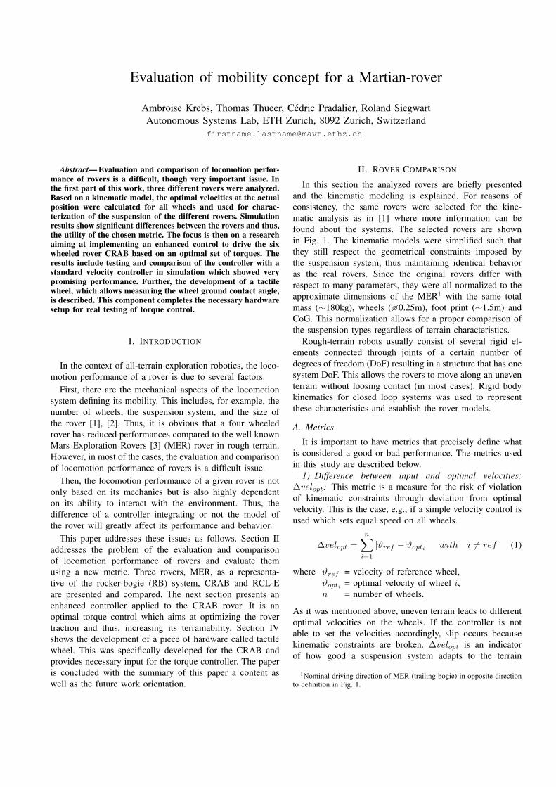
In this section the analyzed rovers are briefly presentedand the kinematic modeling is explained. For reasons ofconsistency, the same rovers were selected for the kine-matic analysis as in [1] where more information can befound about the systems. The selected rovers are shownin Fig. 1. The kinematic models were simplified such thatthey still respect the geometrical constraints imposed bythe suspension system, thus maintaining identical behavioras the real rovers. Since the original rovers differ withrespect to many parameters, they were all normalized to theapproximate dimensions of the MER1 with the same totalmass (∼180kg), wheels (�0.25m), foot print (∼1.5m) andCoG. This normalization allows for a proper comparison ofthe suspension types regardless of terrain characteristics.

Rough-terrain robots usually consist of several rigid el-ements connected through joints of a certain number ofdegrees of freedom (DoF) resulting in a structure that has onesystem DoF. This allows the rovers to move along an uneventerrain without loosing contact (in most cases). Rigid bodykinematics for closed loop systems was used to representthese characteristics and establish the rover models.

A. Metrics

It is important to have metrics that precisely define whatis considered a good or bad performance. The metrics usedin this study are described below.

1) Difference between input and optimal velocities:∆velopt: This metric is a measure for the risk of violationof kinematic constraints through deviation from optimalvelocity. This is the case, e.g., if a simple velocity control isused which sets equal speed on all wheels.

∆velopt =n∑

i=1

|ϑref − ϑopti| with i 6= ref (1)

where ϑref = velocity of reference wheel,ϑopti = optimal velocity of wheel i,n = number of wheels.

As it was mentioned above, uneven terrain leads to differentoptimal velocities on the wheels. If the controller is notable to set the velocities accordingly, slip occurs becausekinematic constraints are broken. ∆velopt is an indicatorof how good a suspension system adapts to the terrain

1Nominal driving direction of MER (trailing bogie) in opposite directionto definition in Fig. 1.

Breadboard Schematic view Kinematic model

Rocker-bogie (MER by NASA)

CRAB by ASL (symmetric structure based on four parallel bogies)

RCL-E by RCL (three parallel bogies, no differential mechanism)

Fig. 1. Selected rovers: MER, CRAB and RCL-E.

while respecting kinematic constraints and not needing asophisticated controller. If this value is small it is easierto control the rover because the kinematics impose similarwheel velocities, and the risk of slip is smaller.

2) Slip: Slip is defined as the difference between the dis-placement of a wheel measured at the wheel center point andthe displacement derived from wheel rotation measurementwith encoders.

slip =n∑

i=1

|∆poswheelcenteri−∆posencoderi

| (2)

Slip is bad for the odometry and it is a waste of energybecause it does not contribute to the movement of the rover.Therefore this value must be small for good performance.

B. Simulation setup

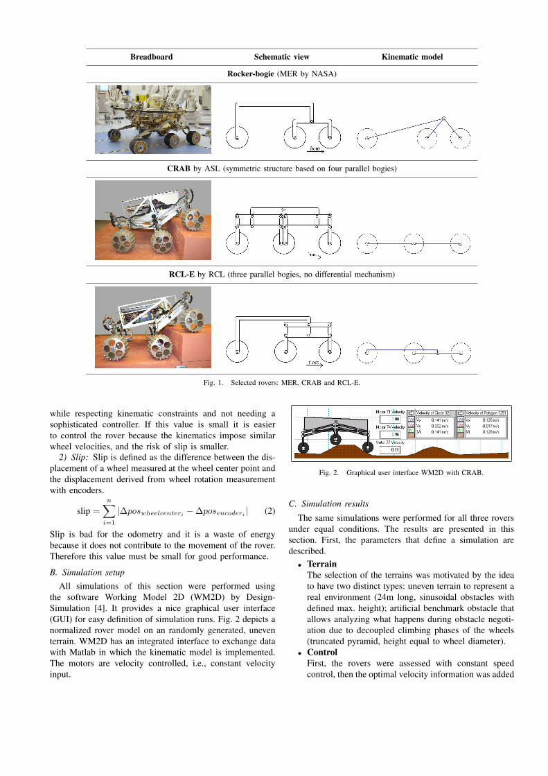
All simulations of this section were performed usingthe software Working Model 2D (WM2D) by Design-Simulation [4]. It provides a nice graphical user interface(GUI) for easy definition of simulation runs. Fig. 2 depicts anormalized rover model on an randomly generated, uneventerrain. WM2D has an integrated interface to exchange datawith Matlab in which the kinematic model is implemented.The motors are velocity controlled, i.e., constant velocityinput.

Fig. 2. Graphical user interface WM2D with CRAB.

C. Simulation results

The same simulations were performed for all three roversunder equal conditions. The results are presented in thissection. First, the parameters that define a simulation aredescribed.

• TerrainThe selection of the terrains was motivated by the ideato have two distinct types: uneven terrain to represent areal environment (24m long, sinusoidal obstacles withdefined max. height); artificial benchmark obstacle thatallows analyzing what happens during obstacle negoti-ation due to decoupled climbing phases of the wheels(truncated pyramid, height equal to wheel diameter).

• ControlFirst, the rovers were assessed with constant speedcontrol, then the optimal velocity information was added

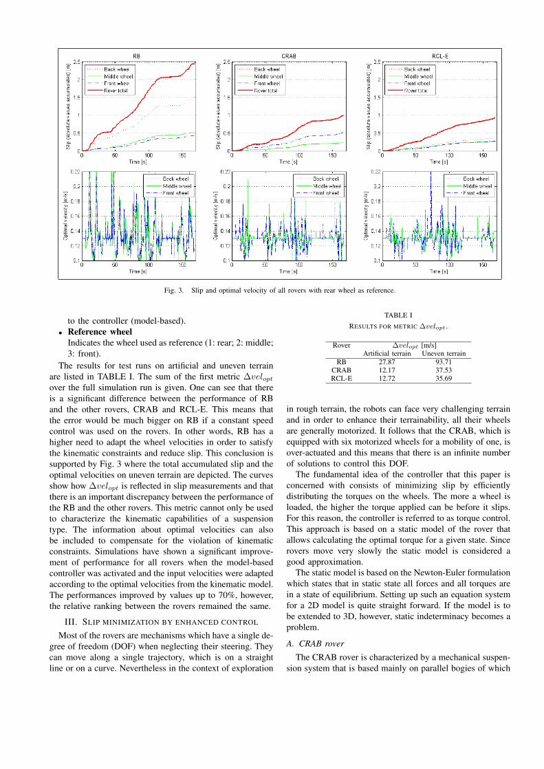
Fig. 3. Slip and optimal velocity of all rovers with rear wheel as reference.

to the controller (model-based).• Reference wheel

Indicates the wheel used as reference (1: rear; 2: middle;3: front).

The results for test runs on artificial and uneven terrainare listed in TABLE I. The sum of the first metric ∆velopt

over the full simulation run is given. One can see that thereis a significant difference between the performance of RBand the other rovers, CRAB and RCL-E. This means thatthe error would be much bigger on RB if a constant speedcontrol was used on the rovers. In other words, RB has ahigher need to adapt the wheel velocities in order to satisfythe kinematic constraints and reduce slip. This conclusion issupported by Fig. 3 where the total accumulated slip and theoptimal velocities on uneven terrain are depicted. The curvesshow how ∆velopt is reflected in slip measurements and thatthere is an important discrepancy between the performance ofthe RB and the other rovers. This metric cannot only be usedto characterize the kinematic capabilities of a suspensiontype. The information about optimal velocities can alsobe included to compensate for the violation of kinematicconstraints. Simulations have shown a significant improve-ment of performance for all rovers when the model-basedcontroller was activated and the input velocities were adaptedaccording to the optimal velocities from the kinematic model.The performances improved by values up to 70%, however,the relative ranking between the rovers remained the same.

III. SLIP MINIMIZATION BY ENHANCED CONTROL

Most of the rovers are mechanisms which have a single de-gree of freedom (DOF) when neglecting their steering. Theycan move along a single trajectory, which is on a straightline or on a curve. Nevertheless in the context of exploration

TABLE IRESULTS FOR METRIC ∆velopt .

Rover ∆velopt [m/s]Artificial terrain Uneven terrain

RB 27.87 93.71CRAB 12.17 37.53RCL-E 12.72 35.69

in rough terrain, the robots can face very challenging terrainand in order to enhance their terrainability, all their wheelsare generally motorized. It follows that the CRAB, which isequipped with six motorized wheels for a mobility of one, isover-actuated and this means that there is an infinite numberof solutions to control this DOF.

The fundamental idea of the controller that this paper isconcerned with consists of minimizing slip by efficientlydistributing the torques on the wheels. The more a wheel isloaded, the higher the torque applied can be before it slips.For this reason, the controller is referred to as torque control.This approach is based on a static model of the rover thatallows calculating the optimal torque for a given state. Sincerovers move very slowly the static model is considered agood approximation.

The static model is based on the Newton-Euler formulationwhich states that in static state all forces and all torques arein a state of equilibrium. Setting up such an equation systemfor a 2D model is quite straight forward. If the model is tobe extended to 3D, however, static indeterminacy becomes aproblem.

A. CRAB rover

The CRAB rover is characterized by a mechanical suspen-sion system that is based mainly on parallel bogies of which

it has two on each side. They are connected at the bottomnext to the axis of the middle wheel and at the top throughan articulated rocker. A differential mechanism between theleft and right suspension levels the pitch angle of the chassis.

The mobility of a rover should be one and can be com-puted with Grubler’s formula [5]:

MO = 6 · n− 5 · f1 − 4 · f2 − 3 · f3 − 2 · f4 − f5 (3)

where MO is the mobility of the system (the rover in thiscase), n the number of mechanical parts and fj the numberof joints of all types (j = 1 . . . 5).

The mechanical structure of the CRAB suspension systemis composed of 30 parts and 41 pivot joints. To that, the sixwheel-ground contacts have to be added which are assumedto be spherical joints (DOF = 3). Using these numbersthe result of Eq. 3 is −43 for the CRAB’s mobility insteadof 1. This result is due to the multiples kinematic loops inthe structure and redundancy of joints that provoke staticindeterminacy. Therefore, the model has to be modifiedin order to conform to the mathematical constraints whilepreserving the real behavior (Fig. 4).

Fig. 4. CRAB rover schematic. All modified DOF joints in the model areindicated by red circles.

The first modification (A) concerns the wheel groundinteraction as only two wheels out of the six can take lateralforces in order to avoid hyperstatism. Thus, four contactsare modeled as joints with 4 DOF instead of three. As aresult only the left front and the right rear wheels take uplateral forces. In a next step (B) three joints of every parallelbogie (green) are given more DOF to be compliant withthe constraints implied by these parallel mechanisms andthe multiple loops induced. The third change (C) affects asingle joint on each side of the structure. It concerns theloop formed by the parallel bogies and the articulated rocker(green and blue). Finally (D), the joints in the loop formedby the differential (yellow), the main body and the structureson both sides are modified to reduce the number of blockedDOF.

These changes lead to a CRAB model with a mobilityof 1. Tests of the model representing various typical roverstates showed that the equation system can be solved and theresults conform to the rover behavior.

B. Equation system

The CRAB consists of 30 parts and can be characterizedby 6*30 = 180 independent equations describing the staticequilibrium of each body and involving 14 external groundforces, 6 internal torques and 165 internal forces for a totalof 185 unknowns. The mechanical structure is consideredmassless whereas the weight of the main body and the wheelsis taken into account.

As no interest is held in the internal variables, it is possibleto simplify the equation system. The variables of interestare the wheel torques and the wheel ground contact forceswhich constitute a total of 20 variables and can be expressedby 25 equations. Nevertheless, the reduction of the systemdimension comes with an increase of equation complexity.For this reason, 23 internal forces remain in the final equationsystem additionally to the forces and torques of interest.

C. Optimization

In order to solve such an equation system n-1 parameterscan be chosen and input to the system (n = number ofwheels). In the torque control algorithm this free choiceis exploited in the sense that the torques are subject to anoptimization algorithm. The criterion for the optimizationcan be described as minimization of the variance of therequired friction coefficient Gi, as illustrated in Eq. 5. Gi isdefined as ratio between tangential Ri and normal Ni contactforce (Eq. 4) and its optimal value is equal for all wheels.The equation for the ith wheel is:

Gi =Ri

Ni(4)

The optimal set of torques ~T ? is determined heuristicallyby Eq. 5 while respecting the mechanical constraints result-ing from the rover structure.

~T ? = arg min~T

(∑i

(Gi(~T )− G(~T )

)2)

(5)

where G is the mean required friction coefficient.This solution has the lowest friction requirements for the

ground. The risk that the rover actually starts to slip in such aposition is minimized although the terrain type is unknown.This solution corresponds to the best possible performanceof the mechanical structure in terms of friction requirement.

D. Simulation

The simulations served several purposes: implementationand testing of the CRAB model; development of the controlalgorithms which will also be used on the breadboard;reproduction of former results adapted to current hardware(CRAB instead of the SOLERO rover [6]).

a) Controller: Different types of controllers for vehi-cles operating in uneven terrain have been proposed. In orderto show the advantages of the traction maximizing control al-gorithm (torque control) it was compared to velocity controlwith wheel synchronization.

b) Torque control: The basic idea of the optimal torquecontrol algorithm is to set torques according to the loaddistribution on the wheels in order to maximize traction. Thestatic model presented above provides the torques that areneeded to maintain the rover in a static state of equilibrium.In order to make the rover move, a PID controller whichtakes the velocity error as input and generates a correctiontorque as output is added to the control loop. The samecontrol scheme as in [6] was used. This is depicted in Fig. 5.

Fig. 5. Control scheme for optimal torques.

c) Wheel velocity synchronization: This algorithm aimsat synchronizing the velocities of all wheels by detectingoutliers, i.e. wheels that rotate at significantly higher speedthan the others. Once the outliers are identified the meanrotation velocity of the wheels can be estimated more accu-rately. Based on the deviation of a wheel’s rotational velocityfrom the estimated mean velocity a velocity correction termcan be calculated [7].

Fig. 6. CRAB rover during simulation.

E. Results

For the simulations, performed in ODE, [8] three differentterrains were used. The rover was tested on all terrains,once with each controller. distance was slightly more than4 m. An example is given in Fig. 7. which depicts thetrajectories of the wheels and the rover body on terrainnumber 3. The terrains differ in number and size of bumpsand are well suited for performance comparison. Threeterrains are certainly not sufficient for a statistically completeanalysis but the tests on those terrains provide enough datato illustrate the potential of torque control on uneven terrain.

The metric for the performance evaluation was slip. Thischoice was motivated by the fact that several aspects of arover mission demand for as little slip as possible. Navigationis more accurate if the rover does not slip; since slippingwheels do not contribute to the rovers movement it is a lossof energy; slip can increase the risk of an operation failuredue to loss of control over the vehicle.

There are two situations where slip occurs: the wheelsare fighting each other due to uneven terrain or differentvelocities; the applied torque is too high and the groundcannot sustain the created traction. Torque control tries toavoid the latter by assigning bigger torques on wheels wherethe load is bigger because more traction can be generated.

The results of the simulations on the three terrains withboth controllers (µ = 0.4) are listed in Table 2. It can beseen that torque control helps reducing slip significantly.The improvement, however, depends on the terrain whichis reflected in a range of 23 to 42% less slip. Even thoughthis range is quite large, it promises a valuable gain in perfor-mance compared to the one of known, existing controllers.

Fig. 7. Wheel and body trajectories on terrain number 3.

The total accumulated slip and the total slip per time stepof all wheels together, while moving over terrain number3, are depicted in Fig. 8. The graphs show the comparisonbetween torque and velocity control, each for a differentfriction coefficient (0.4 to 0.6 top to bottom).

One can see that the rover slips less if driven with torquecontrol but this difference decreases with an increasing fric-tion coefficient. The more traction the ground can provide,the less important becomes the choice of the wheel torques.The remaining slip is mainly caused by wheels rotating atdifferent velocities due to the uneven ground, not by lack oftraction.

TABLE IICOMPARISON OF TOTAL ACCUMULATED SLIP WITH DIFFERENT

CONTROL TYPES AND µ = 0.4 (TOTAL TRAVELED DISTANCE OF ALL

WHEELS TOGETHER ≈ 25m).

Control TypeTerrain Torque Velocity Diff

1 1.41 m 2.41 m 42 %2 1.02 m 1.60 m 37 %3 1.97 m 2.56 m 23 %

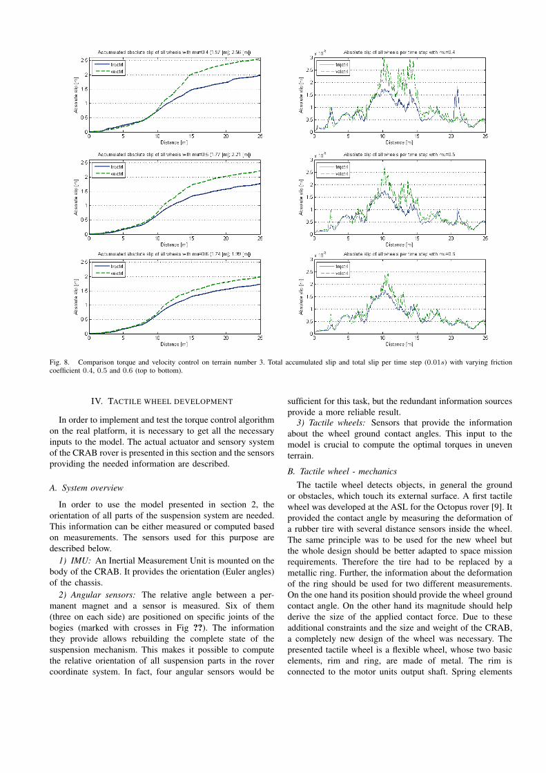
Fig. 8. Comparison torque and velocity control on terrain number 3. Total accumulated slip and total slip per time step (0.01s) with varying frictioncoefficient 0.4, 0.5 and 0.6 (top to bottom).

IV. TACTILE WHEEL DEVELOPMENT

In order to implement and test the torque control algorithmon the real platform, it is necessary to get all the necessaryinputs to the model. The actual actuator and sensory systemof the CRAB rover is presented in this section and the sensorsproviding the needed information are described.

A. System overview

In order to use the model presented in section 2, theorientation of all parts of the suspension system are needed.This information can be either measured or computed basedon measurements. The sensors used for this purpose aredescribed below.

1) IMU: An Inertial Measurement Unit is mounted on thebody of the CRAB. It provides the orientation (Euler angles)of the chassis.

2) Angular sensors: The relative angle between a per-manent magnet and a sensor is measured. Six of them(three on each side) are positioned on specific joints of thebogies (marked with crosses in Fig ??). The informationthey provide allows rebuilding the complete state of thesuspension mechanism. This makes it possible to computethe relative orientation of all suspension parts in the rovercoordinate system. In fact, four angular sensors would be

sufficient for this task, but the redundant information sourcesprovide a more reliable result.

3) Tactile wheels: Sensors that provide the informationabout the wheel ground contact angles. This input to themodel is crucial to compute the optimal torques in uneventerrain.

B. Tactile wheel - mechanicsThe tactile wheel detects objects, in general the ground

or obstacles, which touch its external surface. A first tactilewheel was developed at the ASL for the Octopus rover [9]. Itprovided the contact angle by measuring the deformation ofa rubber tire with several distance sensors inside the wheel.The same principle was to be used for the new wheel butthe whole design should be better adapted to space missionrequirements. Therefore the tire had to be replaced by ametallic ring. Further, the information about the deformationof the ring should be used for two different measurements.On the one hand its position should provide the wheel groundcontact angle. On the other hand its magnitude should helpderive the size of the applied contact force. Due to theseadditional constraints and the size and weight of the CRAB,a completely new design of the wheel was necessary. Thepresented tactile wheel is a flexible wheel, whose two basicelements, rim and ring, are made of metal. The rim isconnected to the motor units output shaft. Spring elements

transmit the torque from the rim to the flexible ring andkeep the two elements at a well defined distance relativeto each other. The selection of the spring elements wascritical since they influence torque transmission and wheeldeformation significantly. Four different concepts were testedand evaluated. They are depicted in Fig. 9: wheels a) andb), called MOVE and Sinus respectively, were developed byDLR [10], while c) and d) are ASL designs [11].

Fig. 9. Four spring concepts studied and tested for use in a metallic flexiblewheel.

The arrangement as well as dimensions and thickness ofthe springs have an impact on the characteristic of the wheel.In order to measure deformations and characterize the wheelsin terms of important properties like linearity and amplitudeof the deformation a test bench was built.

The first inspected feature was the radial deformation ofthe wheel when exerting a radial force on the wheel at dif-ferent angles. The desired characteristic was a homogeneousradial deformation. The second characteristic measured wasthe relative angular displacement of the rim with respect tothe ring when applying a given torque to the rim. In the thirdtest, the axial displacement of the rim with respect to the ringwas determined. Ideally, both values should be as small aspossible.

Another parameter of the wheel design was the numberof rows of springs. Up to three rows with relative angulardisplacements of 30o and 60o were tested. The differentspring concepts were not combined to additional designs.

The forces applied to measure the radial deformation werefrom 20N to 100N in steps of 20N . This order of magnitudewas defined based on simulations of the CRAB on a stepobstacle performed with a 2D simulator [12]. An exampleof the test results is shown in Fig 10.a) and b) for the MOVEwheel and the iWheel12 respectively. It was to be expectedthat the curve of the iWheel12 would be more linear since

it has more springs integrated. However, the tests revealedthat it is necessary to have this number of springs to get thedesired behavior that allows determining the applied forcebased on the amplitude of the deformation. Furthermore, ithas to be pointed out that the design of the MOVE wheeldoes not allow increasing the number of springs enough.

The graphs of Fig 10 have different scales. The defor-mation of the iWheel12 is between 0 and 5.5mm and issmaller compared to the MOVE type results (i.e. between0 and 9mm). The iWheel12 is harder than the MOVEtype wheel, but its deformation is more uniform, which isimportant. While the iWheel12 showed the smallest angulardisplacement in the second test, there were no noticeabledifferences of axial displacement in test three.

The results of the tests show the best performance ofthe iWheel12 with two rows of springs. Since the secondrow of springs points in the opposite direction a Sinus typeconfiguration is formed as can be seen in Figure 11.a). Onlytwo rows of springs are used, whereas it would be necessaryto use four rows of Sinus type springs to have the samenumber of support points on the outer ring.

���

���

���

Fig. 10. Wheel deformation depending on the applied force. a) MOVE (2rows of springs) b) iWheel12 (2 rows of springs) c) illustrates the measuringmechanism.

Fig. 11. iWheel12 flexible wheel a) Front view. b) Rear view with sensorrack.

The selected spring arrangement allows an increase in thenumber of supporting points without the need of adding morerows of springs inside the wheel. Only the number of springs

per row has to be increased. This may be an option if theload on the wheel is increased.

C. Tactile wheel - electronics

To transform the flexible wheel presented in the last sec-tion into a tactile wheel, the deformation has to be measured.Therefore, infrared (IR) distance sensors were integratedinside the wheel. These are able to measure the distance fromthe sensor to the ring. A micro-controller drives the sensorsand calculates the location and the degree of deformation ofthe wheel. Finally, it outputs the wheel ground contact angle.

The selection of IR sensors was a result of a compre-hensive evaluation which included parameters like powerconsumption, size (volume) and mechanical complexity forintegration. Two methods for the measurement of the de-formation were considered. The direct method measures thedistance between ring and rim. Physical principles suited forthis method are return signal intensity measurement (light),triangulation (light), ultrasound, induction and linear poten-tiometer. The indirect method measures the real deformationon the ring or springs, for which strain gages could be used.The return signal intensity measurement was found to be thebest solution for this specific application and the existingconstraints. Inductive sensors are also an excellent meanto perform this task and have the advantage of not beingsensitive to dust. Unfortunately these sensors are spatiallytoo expensive and it would require a specific development.

The rack holding 19 sensors (Fig 11.b) is mounted on thenon rotating part of the wheel assembly. The sensors arepointing downward (Fig.10.c) covering slightly more than180o, which is enough for the presented application. Therack also protects the sensors and limits the deformation ofthe ring.

V. CONCLUSION

In the first part, the rover locomotion performance wasanalyzed from a kinematic point of view. The main focuswas laid on the characterization of suspension systems. Threedifferent systems were compared based on two different met-rics. The new metric ∆velopt was introduced with the aim tocharacterize the suspension systems in terms of compliancewith kinematic constraints while moving on uneven terrain.Slip was used as a second metric because it occurs whenkinematic constraints are violated. The rovers CRAB andRCL-E performed well with respect to both presented metricswhile RB’s performance was significantly inferior.

In the following part, the current state of the CRAB roboticstructure aiming at implementing an enhanced controller,using an optimal torque distribution, was presented. First, therover model was set up which required a significant effortdue to the complexity of the real system. The adaptationwith respect to the real mechanical structure in order toobtain an equivalent model with a mobility of one was anintricate process. This model provides the basis to computethe optimal torques which minimize slip on the rover’swheels. The heuristic for the selection of optimal torquesleading to equal friction requirements on all wheels was

given. The controller itself uses the optimally distributedtorques and adds a correction term based on the rover’svelocity. It was compared to a standard velocity controller. Itshowed very encouraging results. The torque based controllerhad slip values reduced by 23 % to 42 %, depending on thesimulation settings.

As this controller is supposed to be used on the real CRABrover in the near future, the hardware has to provide allthe necessary information which describes the rover’s state.The last part of this paper presents the sensors available aswell as the development of a tactile wheel. It is based ona flexible wheel whose deformation is measured to providethe wheel-ground contact angle. The next step lies in actuallyintegrating the controller on the real platform and testing it.All the various components are now available, only theirintegration on the CRAB is missing. This is one of the mainobjectives of future research at ASL.

REFERENCES

[1] T. Thueer, A. Krebs, P. Lamon, and R. Siegwart, “Performancecomparison of rough-terrain robots - simulation and hardware,” In-ternational Journal of Field Robotics Vol.24 Issue 3 (Special Issue onSpace Robotics Part I), Wiley, 2007.

[2] T. Thueer, A. Krebs, and R. Siegwart, “Comprehensive locomotionperformance evaluation of all-terrain robots,” in IEEE InternationalConference on Intelligent Robots and Systems (IROS’06), Beijing,China, 2006.

[3] R. A. Lindemann and C. J. Voorhees, “Mars exploration rover mo-bility assembly design, test and performance,” in IEEE InternationalConference on Systems, Man and Cybernetics, 2005, vol. 1, Waikoloa,Hawaii, USA, 2005, pp. 450–455.

[4] Design-Simulation, “Working model 2d, http://www.design-simulation.com/wm2d/,” 2006.

[5] M. Grubler, Getriebelehre: Eine Theorie des Zwanglaufes und derebenen Mechanismen. Springer, 1917.

[6] P. Lamon and R. Siegwart, “Wheel torque control in rough terrain -modeling and simulation,” in ICRA, Barcelona, Spain, 2005.

[7] E. T. Baumgartner and H. Aghazarian, “Rover localization results forthe fido rover.” SPIE 4571: 34-44., 2001.

[8] Http://ode.org.[9] M. Lauria, Y. Piguet, and R. Siegwart, “Octopus: An aoutonomous

wheeled climbing robot,” 2002.[10] Http://www.rcom.marum.de/Moving Lander.html.[11] E. Carrasco, “Development of tactile wheel for space application,”

2007, master Thesis, ETHZ, April.[12] A. Krebs, T. Thuer, and R. Siegwart, “Performance optimization of

all-terrain robots: A 2d quasi-static tool,” in IROS, Beijing, China,2005.