Evaluation of Local 3-D Point Cloud Descriptors in Terms of Suitabilityfor Object Classification

Jens Garstka and Gabriele PetersHuman-Computer Interaction, Faculty of Mathematics and Computer Science,

University of Hagen, D-58084 Hagen, Germany{jens.garstka, gabriele.peters}@fernuni-hagen.de

Keywords: Local 3-D Feature Descriptors, Performance Evaluation, Object Classification.

Abstract: This paper investigates existing methods for local 3-D feature description with special regards to their suitabil-ity for object classification based on 3-D point cloud data. We choose five approved descriptors, namely SpinImages, Point Feature Histogram, Fast Point Feature Histogram, Signature of Histograms of Orientations, andUnique Shape Context and evaluate them with a commonly used classification pipeline on a large scale 3-Dobject dataset comprising more than 200000 different point clouds. Of particular interest are the details of thechoice of all parameters associated with the classification pipeline. The point clouds are classified by usingsupport vector machines. Fast Point Feature Histogram proves to be the best descriptor for the method ofobject classification used in this evaluation.

1 INTRODUCTION

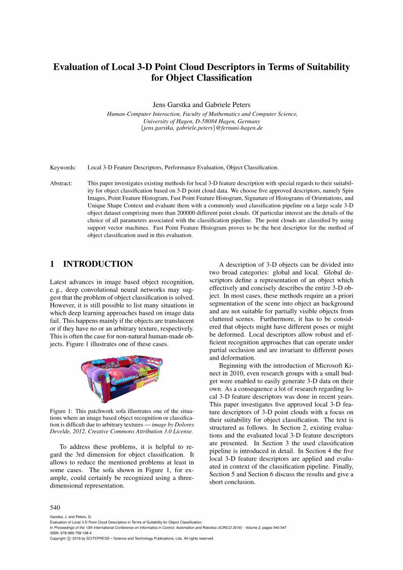
Latest advances in image based object recognition,e. g., deep convolutional neural networks may sug-gest that the problem of object classification is solved.However, it is still possible to list many situations inwhich deep learning approaches based on image datafail. This happens mainly if the objects are translucentor if they have no or an arbitrary texture, respectively.This is often the case for non-natural human-made ob-jects. Figure 1 illustrates one of these cases.

Figure 1: This patchwork sofa illustrates one of the situa-tions where an image based object recognition or classifica-tion is difficult due to arbitrary textures — image by DoloresDevelde, 2012, Creative Commons Attribution 3.0 License.

To address these problems, it is helpful to re-gard the 3rd dimension for object classification. Itallows to reduce the mentioned problems at least insome cases. The sofa shown in Figure 1, for ex-ample, could certainly be recognized using a three-dimensional representation.

A description of 3-D objects can be divided intotwo broad categories: global and local. Global de-scriptors define a representation of an object whicheffectively and concisely describes the entire 3-D ob-ject. In most cases, these methods require an a priorisegmentation of the scene into object an backgroundand are not suitable for partially visible objects fromcluttered scenes. Furthermore, it has to be consid-ered that objects might have different poses or mightbe deformed. Local descriptors allow robust and ef-ficient recognition approaches that can operate underpartial occlusion and are invariant to different posesand deformation.

Beginning with the introduction of Microsoft Ki-nect in 2010, even research groups with a small bud-get were enabled to easily generate 3-D data on theirown. As a consequence a lot of research regarding lo-cal 3-D feature descriptors was done in recent years.This paper investigates five approved local 3-D fea-ture descriptors of 3-D point clouds with a focus ontheir suitability for object classification. The text isstructured as follows. In Section 2, existing evalua-tions and the evaluated local 3-D feature descriptorsare presented. In Section 3 the used classificationpipeline is introduced in detail. In Section 4 the fivelocal 3-D feature descriptors are applied and evalu-ated in context of the classification pipeline. Finally,Section 5 and Section 6 discuss the results and give ashort conclusion.

540Garstka, J. and Peters, G.Evaluation of Local 3-D Point Cloud Descriptors in Terms of Suitability for Object Classification.In Proceedings of the 13th International Conference on Informatics in Control, Automation and Robotics (ICINCO 2016) - Volume 2, pages 540-547ISBN: 978-989-758-198-4Copyright c© 2016 by SCITEPRESS – Science and Technology Publications, Lda. All rights reserved

2 RELATED WORK

Subsequently, already published evaluations of local3-D feature descriptors and the local 3-D feature de-scriptions considered in this paper are introduced.

2.1 Existing Evaluations

There is a number of publications that deal with evalu-ations of 3-D feature descriptors in the last five years.A survey and evaluation of local shape descriptors(Heider et al., 2011) divides existing local descriptorsinto three classes. Focus of the evaluation are 3-Dmeshes and only local shape descriptors for meshesare examined.

The evaluation of local shape descriptors for 3-Dshape retrieval (Tang and Godil, 2012) is similar tothe work of (Heider et al., 2011), with the differencethat they perform the tests of 6 simple mesh descrip-tors on the SHREC 2011 Shape Retrieval Contest ofNon-rigid 3D Watertight Meshes dataset (Lian et al.,2011).

An evaluation from Alexandre with focus on local3-D descriptors for object and category recognition(Alexandre, 2012) is the publication that is themati-cally most similar to our work. The tested algorithmsare the same ones as those examined in this paper.However, the pipeline proposed by Alexandre is un-suitable for a larger amount of data.

The evaluation of local 3-D feature descriptors fora classification of surface geometries in point clouds(Arbeiter et al., 2012) investigates how local 3-D fea-ture descriptions can be used to classify primitive lo-cal surfaces such as cylinders, edges, or corners inpoint clouds. Arbeiter et al. compare a small selec-tion of three local 3-D feature descriptors.

The goal of the evaluation of 3-D feature descrip-tors in the work of (Kim and Hilton, 2013) is a multi-modal registration of 3-D point clouds, meshes, andimages. Although the descriptors used in this workare the same as in this paper, conclusions regardinga classification of 3-D point clouds can hardly be de-rived from their results.

Finally, a survey on 3-D object recognition in clut-tered scenes with local surface features (Guo et al.,2014) provides a good overview of the available de-scriptors and divides them with a taxonomy into dif-ferent descriptor types. In addition, there is an infor-mal comparison of the performance of each descrip-tor, which, however, is based on the statements givenin each individual publication and not on an own eval-uation.

2.2 Local 3-D Feature Descriptors

The goal of local 3-D feature descriptors is the de-scription of particularly “interesting” local areas of a3-D object. The advantages of local representationsconsist in their robustness with respect to noise, andtheir variability concerning object shape and partialocclusions. A wide variety of methods exists (Guoet al., 2014), but not all are suitable for 3-D pointclouds, but rather meshes or depth images. The fol-lowing five local 3-D feature descriptors are suitablefor the local description of 3-D point clouds and areevaluated in this paper.

The Spin Image (SI) descriptor (Johnson andHebert, 1998; Johnson and Hebert, 1999) is arguablythe most cited and approved local 3-D descriptor. Itis a histogram based method that requires a normalvector as a rotation axis. In a nutshell, all 3-D pointsof the local environment are collected while the 2-Dhistogram is rotated around the normal vector.

The Point Feature Histogram (PFH) (Rusu et al.,2008a) is a histogram based approach as well. Rusuet al. compute Darboux frames (Rusu et al., 2008a)for each 3-D point of a local spherical environment.The three angles of each Darboux frame are subdi-vided into 5 intervals and filled in a histogram with125 bins.

Since the computational complexity for the deter-mination of Darboux frames at each point within ak-neighborhood is O(k2), the computation of PFH isrelatively slow. For this reason, Rusu et al. proposeda simplified version of PFH named Fast Point Fea-ture Histogram (FPFH) (Rusu et al., 2009). They pre-served the basic characteristics of the descriptor, butreplaced the computation of the Darboux frame withan approximation of it.

Tombari et al. propose a descriptor called Signa-tures of Histograms of Orientations (SHOT) (Tombariet al., 2010b; Salti et al., 2014). A spherical neigh-borhood is divided into several segments. For eachsegment a histogram is filled with the cosine valuesof the angles between the z-axis of the local referenceframe and the normal vectors of all points that are partof the currently considered segment.

Another local 3-D feature descriptor introducedby Tombari et al. is Unique Shape Context (USC)(Tombari et al., 2010a). It is an extension of the 3-DShape Context (3DSC) (Frome et al., 2004), whichessentially consists of a spherical histogram dividedinto radial, elevation, and azimuth divisions. Tombariet al. determine a unique local reference frame to en-sure that the histogram has unique orientation.

Evaluation of Local 3-D Point Cloud Descriptors in Terms of Suitability for Object Classification

541

KeypointSelection

FeatureDescriptionPoint Cloud Bag of Words Classification

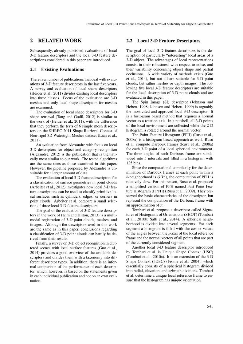
Figure 2: The classification pipeline used for the evaluation of local 3-D feature descriptors. It consists of four main steps:keypoint selection, feature descriptions, a bag-of-words model, and the classification.

3 CLASSIFICATION PIPELINE

At a conceptual level, a 3-D classification pipeline isbased on four main steps. These are the keypoint se-lection (Salti et al., 2011; Dutagaci et al., 2012; Filipeand Alexandre, 2013), the extraction of local featuredescriptions (Alexandre, 2012; Guo et al., 2014), abag-of-words model (Wu and Lin, 2011; Cholewa andSporysz, 2014), and a machine learning method forthe classification task for which support vector ma-chines (Toldo et al., 2010) are widely used. Figure 2depicts these steps with a conceptual illustration ofsuch a pipeline. The individual steps and their param-eters are discussed in detail in the next subsections.

3.1 Point Clouds

The dataset used in the context of this work is theRGB-D Object Dataset (Lai et al., 2011). The datasetcontains 51 object classes, e. g., banana, calculator,glue stick, or sponge. Each object class comprisesseveral different objects of the same object class. Theobject class coffee mug, for example, contains 8 dif-ferent types of coffee cups. In summary, the datasetscontains 300 different objects where each object wascaptured in different poses. This results in 207841distinct point clouds. The mean point cloud resolu-tion (pcr) of these point clouds is ≈ 0.001295.

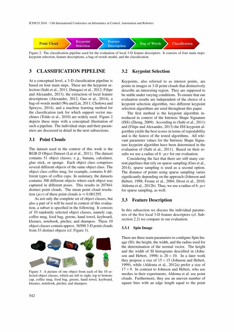
As not only the complete set of object classes, butalso a part of it will be used in context of this evalua-tion, a subset is specified in the following. It consistsof 10 randomly selected object classes, namely cap,coffee mug, food bag, greens, hand towel, keyboard,kleenex, notebook, pitcher, and shampoo. These 10object classes contain approx. 36500 3-D point cloudsfrom 53 distinct objects (cf. Figure 3).

Figure 3: A picture of one object from each of the 10 se-lected object classes, which are left to right, top to bottom:cap, coffee mug, food bag, greens, hand towel, keyboard,kleenex, notebook, pitcher, and shampoo.

3.2 Keypoint Selection

Keypoints, also referred to as interest points, arepoints in images or 3-D point clouds that distinctivelydescribe an interesting region. They are supposed tobe stable under varying conditions. To ensure that ourevaluation results are independent of the choice of akeypoint selection algorithm, two different keypointselection algorithms are used throughout this paper.

The first method is the keypoint algorithm in-troduced in context of the Intrinsic Shape Signature(ISS) (Zhong, 2009). According to (Salti et al., 2011)and (Filipe and Alexandre, 2013) the ISS keypoint al-gorithm yields the best scores in terms of repeatabilityand is the fastest of the tested algorithms. All rele-vant parameter values for the Intrinsic Shape Signa-ture keypoint algorithm have been determined in theevaluation of (Salti et al., 2011). Based on their re-sults we use a radius of 6 · pcr for our evaluation.

Considering the fact that there are still many cur-rent pipelines that rely on sparse sampling (Guo et al.,2014), sparse sampling is used as a second option.The distance of points using sparse sampling variessignificantly depending on the approach (Johnson andHebert, 1998; Frome et al., 2004; Drost et al., 2010;Aldoma et al., 2012b). Thus, we use a radius of 6 · pcrfor sparse sampling, as well.

3.3 Feature Description

In this subsection we discuss the individual parame-ters of the five local 3-D feature descriptors (cf. Sub-section 2.2) we compare in our evaluation.

3.3.1 Spin Image

There are three main parameters to configure Spin Im-age (SI): the height, the width, and the radius used forthe determination of the normal vector. The heightand the width of SI histograms described in (John-son and Hebert, 1998) is 20× 10. In a later workthey propose a size of 15× 15 (Johnson and Hebert,1999), while (Aldoma et al., 2012a) prefer a size of17× 9. In contrast to Johnson and Hebert, who usemeshes in their experiments, Aldoma et al. use pointclouds. Furthermore, they use an uneven number ofsquare bins with an edge length equal to the point

ICINCO 2016 - 13th International Conference on Informatics in Control, Automation and Robotics

542

cloud resolution to take account of the sparse distri-bution of point clouds. Therefore, we decided to fol-low Aldoma et al. and use spin images with a size of17×9 = 153 bins for our evaluation. The normal vec-tor will be calculated based on the same radius usedto compute the histogram: 9 · pcr.

3.3.2 Point Feature Histogram

PFH requires two radii, the spherical support area anda radius to approximate the normal vectors of the Dar-boux frames. The size of the spherical support ar-eas, i. e., the k-neighborhoods, are given by (Rusuet al., 2008a) in meters and centimeters within an in-terval of [2.0cm,3.5cm] for an indoor kitchen sceneand [50cm,150cm] for an outdoor urban scene. Ourtest data mainly includes household objects with asize of at most 30cm. Thus, we can assume that lo-cal features can be limited to a size of 5cm or a k-neighborhood with a radius of 2.5cm, which fits tothe radii that are used by Rusu et al. for the kitchenscene and is approximately equivalent to 19.3 · pcr.

An indication of the size of the area used forthe approximation of the normal vectors is given by(Alexandre, 2012). He proposes a radius of 1cmwhich is ≈ 7.7 · pcr in our dataset. Therefore, we usea radius of 20 · pcr for the spherical support area, anda radius of 8 · pcr to approximate the normal vector.

3.3.3 Fast Point Feature Histogram

As the Fast Point Feature Histogram (Rusu et al.,2009) is based on the Point Feature Histogram andfollows the same mechanism, we use the same radiias for the Point Feature Histogram.

3.3.4 Signatures of Histograms of Orientations

(Tombari et al., 2010b) recommend histograms with11 bins and a segmentation of the spherical environ-ment with 8 azimuth divisions, 2 elevation divisions,and 2 radial divisions. Additionally, Tombari et al.specify the size of the support area with 15 · pcr. Wewill use all these parameter values for our evaluation,too.

3.3.5 Unique Shape Context

All required parameter values for USC are given by(Tombari et al., 2010a): 10 radial divisions, 14 az-imuth divisions, and 14 elevation divisions. The outerradius of the spherical histogram is 20 · pcr, the innerradius of the spherical histogram is 2 · pcr, the radiusto approximate the normal vector is 20 · pcr, and thedensity radius is 2 · pcr. We use these values in ourevaluations as well.

3.4 Bag-of-words

A bag-of-words model is used to count the occur-rences of words of a text in a histogram. In the sameway a bag-of-words model can be used to count theoccurrences of local feature descriptions. In this con-text it is often called a bag-of-features.

The only parameter required in advance is thenumber of bins of the histogram. For each bin, a rep-resentative local 3-D feature description is required.These descriptions are taken from the centers of eachcluster determined by k-means clustering on precom-puted local 3-D feature descriptions. The initial cen-ters of the clusters are chosen at random by using ak-means variant named k-means++ (Arthur and Vas-silvitskii, 2007). The distance measure used is theEuclidean distance.

Depending on the referred source, the selectednumber of clusters k differs by orders of magnitude.Toldo et al. use values of k between 20 and 80 (Toldoet al., 2009) and values from 50 to 150 (Toldo et al.,2010), Knopp et al. use 10% of all feature descriptionsextracted from a training set as a value of k (Knoppet al., 2010). Madry et al. use between 7 and 300clusters (Madry et al., 2012; Madry et al., 2013) andYi et al. use 20% of the average number of featuresthey extracted for each patch of all objects in theirtraining set (Yi et al., 2014). For this reason, 7 dif-ferent histogram sizes, i. e., 10, 20, 50, 100, 200, 500,and 1000 will be compared in this evaluation.

3.5 Classification

Most of the classification approaches in (Toldo et al.,2009; Toldo et al., 2010; Knopp et al., 2010; Madryet al., 2012; Madry et al., 2013; Seib et al., 2013; Yiet al., 2014) use support vector machines as underly-ing technique. Only the approach proposed by Yi isbased on a different concept using a language model.

Rusu et al. state, that support vector machineshave already been used for a classification based ona bag-of-features model for color images with greatsuccess (Rusu et al., 2008b; Rusu, 2010). In the refer-enced works, Rusu et al. test support vector machines,k-nearest neighbor searches, and k-means clusteringin different configurations against each other. Thebest results are achieved using an SVM with a ra-dial basis function (RBF) as kernel. There are someother approaches, e. g., the work presented by (Laiet al., 2011), where in some cases an alternative ma-chine learning approach leads to slightly better re-sults. However, since SVMs are the most widelyused classification method in this problem domain,the evaluation presented here will also use SVMs as

Evaluation of Local 3-D Point Cloud Descriptors in Terms of Suitability for Object Classification

543

binary classifier for each object class. Accordingly, aGaussian radial basis function is used as kernel.

3.6 Summary

In summary, for a given 3-D point cloud we ex-tract a set of keypoints with ISS and sparse sam-pling. For each keypoint we compute a local 3-D fea-ture description based on one of the five selected al-gorithms and determine the nearest representative tocount the feature description in the corresponding binof the bag-of-features histogram. Finally, the bag-of-features histogram is used as input vector for the SVMof each object class and the best matching object classis selected based on the SVM responses.

4 EVALUATION

In this section the evaluation of local 3-D feature de-scriptors is presented in detail. Initially, the most ap-propriate keypoint algorithm, the optimal size of abag-of-features histogram, and the best SVM trainingparameters are determined. This is done in Subsec-tion 4.1, 4.2, and 4.3. In these subsections, all pipelineparameters are optimized to maximize the correct as-signment of an object corresponding to object class Cto C. Subsequently, Subsection 4.4 merges these opti-mizations to an overall classification. Subsection 4.5examines the computation times required to classify3-D point clouds this way.

4.1 SVM-parameters

A Gaussian radial basis functionK(xi,x j) = e−γ‖xi−x j‖2 ,γ > 0

requires the specification of a single parameter γwhich has to be determined depending on the datawhich is used to train the support vector machine. Ad-ditionally, the support vector machine requires a pa-rameter C > 0, which is the penalty parameter of theerror term, i. e., a multiplier of the distance of mis-classified samples to their region.

A Note on SVM Training Histograms:

The following subsections contain small SVM train-ing histograms with the size of 4× 4 bins. All thesehistograms have the same axes and labels. To retainreadability, the axes and labels are not included foreach histogram. Instead, the labels and axes of allhistograms are shown only once in Figure 4. The val-ues of C increase from left to right, while the valuesof γ increase from top to bottom.

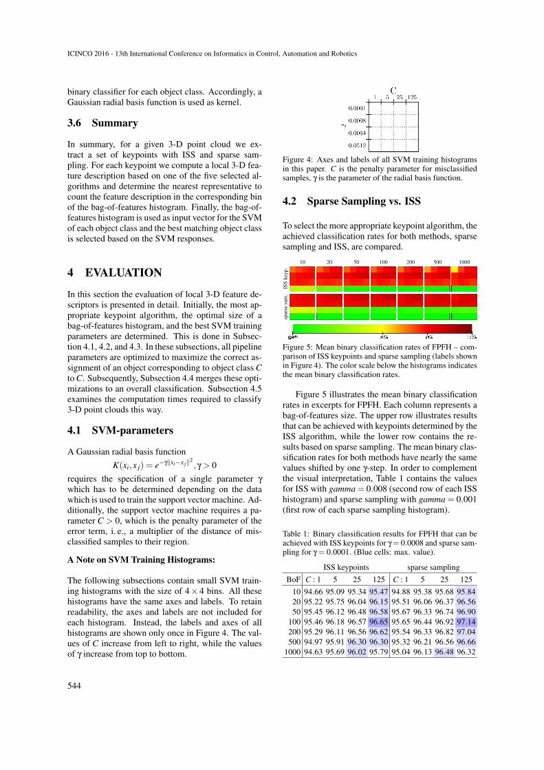
Figure 4: Axes and labels of all SVM training histogramsin this paper. C is the penalty parameter for misclassifiedsamples, γ is the parameter of the radial basis function.

4.2 Sparse Sampling vs. ISS

To select the more appropriate keypoint algorithm, theachieved classification rates for both methods, sparsesampling and ISS, are compared.

10 20 50 100 200 500 1000

ISS

keyp

.sp

arse

sam

.

Figure 5: Mean binary classification rates of FPFH – com-parison of ISS keypoints and sparse sampling (labels shownin Figure 4). The color scale below the histograms indicatesthe mean binary classification rates.

Figure 5 illustrates the mean binary classificationrates in excerpts for FPFH. Each column represents abag-of-features size. The upper row illustrates resultsthat can be achieved with keypoints determined by theISS algorithm, while the lower row contains the re-sults based on sparse sampling. The mean binary clas-sification rates for both methods have nearly the samevalues shifted by one γ-step. In order to complementthe visual interpretation, Table 1 contains the valuesfor ISS with gamma = 0.008 (second row of each ISShistogram) and sparse sampling with gamma = 0.001(first row of each sparse sampling histogram).

Table 1: Binary classification results for FPFH that can beachieved with ISS keypoints for γ = 0.0008 and sparse sam-pling for γ = 0.0001. (Blue cells: max. value).

ISS keypoints sparse samplingBoF C : 1 5 25 125 C : 1 5 25 125

10 94.66 95.09 95.34 95.47 94.88 95.38 95.68 95.8420 95.22 95.75 96.04 96.15 95.51 96.06 96.37 96.5650 95.45 96.12 96.48 96.58 95.67 96.33 96.74 96.90

100 95.46 96.18 96.57 96.65 95.65 96.44 96.92 97.14200 95.29 96.11 96.56 96.62 95.54 96.33 96.82 97.04500 94.97 95.91 96.30 96.30 95.32 96.21 96.56 96.66

1000 94.63 95.69 96.02 95.79 95.04 96.13 96.48 96.32

ICINCO 2016 - 13th International Conference on Informatics in Control, Automation and Robotics

544

The differences in classification rates between ISSand sparse sampling are always less than 0.5%. Thiscannot be denoted as significant. For this reason, thenumber of keypoints should be considered with re-spect to the computation time. The average numberof approx. 355 keypoints per point cloud identifiedby sparse sampling is more than two and a half timeshigher, than the average number of approx. 132 key-points determined by ISS. Accordingly, sparse sam-pling will not be used due to the larger number of fea-tures to be calculated.

4.3 Local 3-D Feature Descriptors

10 20 50 100 200 500 1000

SIPF

HFP

FHSH

OT

USC

Figure 6: Mean binary classification rates of all evaluatedlocal 3-D feature descriptors (labels shown in Figure 4).The color scale below the histograms indicates the meanbinary classification rates.

Figure 6 illustrates the binary classification resultsfor different local 3-D feature descriptors. The lowclassification results of SI are immediately apparent.Additionally, the darkest shade of red indicating thebest classification results can be found for C = 125(right column) and γ = 0.0008 (second row) of eachhistogram. Table 2 summarizes the best configura-tion of parameters for each of the evaluated local 3-Dfeature descriptors, as well as the corresponding clas-sification rates.

Table 2: Classification rate of the considered descriptorswith final set of pipeline parameters. (KP: keypoint algo-rithm, BoF: size of bag-of-features).

KP BoF C γ rateSI ISS 50 125 0.008 92.80%PFH ISS 100 125 0.008 96.56%FPFH ISS 100 125 0.008 96.65%SHOT ISS 100 125 0.008 96.27%USC ISS 200 125 0.008 97.62%

4.4 Overall Classification Results

The mean binary classification rates shown so far,consider only how well an object corresponding toobject class C is correctly assigned to C. In prac-tice, however, it is decisive how often an object cor-responding to object class C is incorrectly assigned toanother objects class C′. This value is relatively highdue to the fact that the shapes of many objects are verysimilar. Thus, the overall classification rate is by farlagging behind the mean binary classification rate ofapprox. 96%. In fact, an exact assignment (a pointcloud is only assigned to the correct object class andall other SVMs reject the point cloud) can neither beachieved considered all 51 object classes, nor whileusing the subset of 10 object classes (see Section 3.1).

However, when choosing only that object classwhere the corresponding SVM returns the highestdistance between the input vector (i. e., the bag-of-features histogram) with respect to the separating hy-perplane, the classification rates shown in Table 3 canbe achieved. Above that, the classification rates thatcan be achieved for 10 object classes are only slightlylower than those that were achieved by (Alexandre,2012).

Table 3: Overall classification rates that can be achievedconsidering the highest distance between the input vectorand the separating hyperplane for each SVM.

51 classes 10 classesSI 7.4% 23.8%PFH 6.0% 62.9%FPFH 9.4% 65.0%SHOT 3.6% 22.8%USC 8.5% 59.7%

4.5 Computation Times

The computation times of the five local 3-D featuredescriptors may be of particular interest to select oneof these algorithms depending on the requirements.Table 4 gives a brief overview of the system used forall computations.

Table 4: System used for evaluation.

ConfigurationCPU Intel Xeon E5630 @2.53GHzMemory 12GB DDR3 @1066MHzOS Debian 8.0 GNU/Linux 64bit

The average computation times to classify a 3-Dpoint cloud with one of the five local 3-D feature de-scriptors are shown in Table 5. The values reflect the

Evaluation of Local 3-D Point Cloud Descriptors in Terms of Suitability for Object Classification

545

computation times that are required for classification.The computation of keypoints, local 3-D feature vec-tors, and bag-of-feature are not taken into account.

Table 5: Average classification times. The values indicatethe time to classify the bag-of-features histogram withineach SVM.

10 classes all 51 classesSI ≈ 2.13ms ≈ 10.9msPFH ≈ 7.40ms ≈ 37.8msFPFH ≈ 2.29ms ≈ 11.7msSHOT ≈ 5.85ms ≈ 29.8msUSC ≈ 3.40ms ≈ 17.3ms

Table 6 shows the mean computation times of asingle local 3-D feature description and a factor thatenables a quick comparison of the computation timeswith respect to the fastest algorithm SI.

Table 6: Computation times of 3-D feature description al-gorithms used within the experiments in ascending order.The last column shows the factor with respect to the fastestalgorithm SI.

Time FactorSI ≈ 0.045ms 1SHOT ≈ 0.28ms ≈ 6FPFH ≈ 6.69ms ≈ 150USC ≈ 9.95ms ≈ 220PFH ≈ 64.51ms ≈ 1430

5 DISCUSSION

Our evaluation of five local 3-D feature descriptorswith a focus on 3-D object classification shows, thatit is possible to achieve approx. 60% to 65% correctclass assignments with PFH, FPFH, and USC (cf. Ta-ble 3). The two other algorithms, SI and the SHOTachieve classification rates of only 22% and 23%.In case of SI the mean binary classification rate of92.80% is considerably lower compared to the otheralgorithms. The reason for the bad results of SHOTremains unclear. Considering the algorithms with re-spect to the computation and classification times, SIand SHOT are by far the fastest methods (cf. Table 5and 6). However, the classification rates of these twoalgorithms are so low that the two algorithms shouldnot be used in this context. Of the remaining three al-gorithms FPFH is the fastest and best method, i. e., themethod with the highest classification rate at the sametime. However, considering the classification resultsof all local 3-D feature descriptors in context of thefull test dataset using all 51 object classes (cf. Table 3)it turns out that a classification of 3-D objects, that are

almost indistinguishable in terms of shape, is in factnot possible. For this reason, the use of local 3-Dfeatures can only be seen as a complement to color-based object classification. This is in particular thecase when ambiguous textures or bad lighting condi-tions complicate a color image based method.

6 CONCLUSION

Summarizing, the Fast Point Feature Histogram pro-vides the best results in terms of computation time andclassification rate. However, it has to be taken into ac-count that an object classification on the sole basis of3-D representations only works when the classes aresufficiently different.

REFERENCES

Aldoma, A., Marton, Z.-C., Tombari, F., Wohlkinger, W.,Potthast, C., Zeisl, B., Rusu, R., Gedikli, S., andVincze, M. (2012a). Tutorial: Point cloud library:Three-dimensional object recognition and 6 dof poseestimation. Robotics Automation Magazine, IEEE,19(3):80–91.

Aldoma, A., Tombari, F., Rusu, R. B., and Vincze, M.(2012b). Our-cvfh–oriented, unique and repeat-able clustered viewpoint feature histogram for ob-ject recognition and 6dof pose estimation. In PatternRecognition, pages 113–122. Springer.

Alexandre, L. A. (2012). 3d descriptors for object and cate-gory recognition: a comparative evaluation. In Work-shop on Color-Depth Camera Fusion in Robotics atthe IEEE/RSJ International Conference on IntelligentRobots and Systems (IROS), Vilamoura, Portugal.

Arbeiter, G., Fuchs, S., Bormann, R., Fischer, J., and Verl,A. (2012). Evaluation of 3d feature descriptors forclassification of surface geometries in point clouds.In 2012 IEEE/RSJ International Conference on In-telligent Robots and Systems, IROS 2012, Vilamoura,Algarve, Portugal, October 7-12, 2012, pages 1644–1650.

Arthur, D. and Vassilvitskii, S. (2007). k-means++: Theadvantages of careful seeding. In Proceedings of theeighteenth annual ACM-SIAM symposium on Discretealgorithms, pages 1027–1035. Society for Industrialand Applied Mathematics.

Cholewa, M. and Sporysz, P. (2014). Classification of dy-namic sequences of 3d point clouds. In Artificial Intel-ligence and Soft Computing, pages 672–683. Springer.

Drost, B., Ulrich, M., Navab, N., and Ilic, S. (2010). Modelglobally, match locally: Efficient and robust 3d objectrecognition. In Computer Vision and Pattern Recogni-tion (CVPR), 2010 IEEE Conference on, pages 998–1005. IEEE.

Dutagaci, H., Cheung, C. P., and Godil, A. (2012). Eval-uation of 3d interest point detection techniques via

ICINCO 2016 - 13th International Conference on Informatics in Control, Automation and Robotics

546

human-generated ground truth. The Visual Computer,28(9):901–917.

Filipe, S. and Alexandre, L. A. (2013). A comparative eval-uation of 3d keypoint detectors. In 9th Conference onTelecommunications, Conftele 2013, pages 145–148,Castelo Branco, Portugal.

Frome, A., Huber, D., Kolluri, R., Bulow, T., and Malik,J. (2004). Recognizing objects in range data usingregional point descriptors. In Proceedings of the Eu-ropean Conference on Computer Vision (ECCV).

Guo, Y., Bennamoun, M., Sohel, F., Lu, M., and Wan,J. (2014). 3d object recognition in cluttered sceneswith local surface features: A survey. Pattern Analy-sis and Machine Intelligence, IEEE Transactions on,36(11):2270–2287.

Heider, P., Pierre-Pierre, A., Li, R., and Grimm, C. (2011).Local shape descriptors, a survey and evaluation. InProceedings of the 4th Eurographics conference on3D Object Retrieval, pages 49–56. Eurographics As-sociation.

Johnson, A. and Hebert, M. (1999). Using spin images forefficient object recognition in cluttered 3d scenes. Pat-tern Analysis and Machine Intelligence, IEEE Trans-actions on, 21(5):433–449.

Johnson, A. E. and Hebert, M. (1998). Surface matchingfor object recognition in complex three-dimensionalscenes. Image and Vision Computing, 16(9):635–651.

Kim, H. and Hilton, A. (2013). Evaluation of 3d feature de-scriptors for multi-modal data registration. In 2013 In-ternational Conference on 3D Vision, 3DV 2013, Seat-tle, Washington, USA, June 29 - July 1, 2013, pages119–126.

Knopp, J., Prasad, M., Willems, G., Timofte, R., andVan Gool, L. (2010). Hough transform and 3d surf forrobust three dimensional classification. In ComputerVision–ECCV 2010, pages 589–602. Springer.

Lai, K., Bo, L., Ren, X., and Fox, D. (2011). A large-scale hierarchical multi-view rgb-d object dataset. InRobotics and Automation (ICRA), 2011 IEEE Interna-tional Conference on, pages 1817–1824. IEEE.

Lian, Z., Godil, A., Bustos, B., Daoudi, M., Hermans, J.,Kawamura, S., Kurita, Y., Lavoue, G., Van Nguyen,H., Ohbuchi, R., et al. (2011). Shrec’11 track: Shaperetrieval on non-rigid 3d watertight meshes. 3DOR,11:79–88.

Madry, M., Afkham, H. M., Ek, C. H., Carlsson, S., andKragic, D. (2013). Extracting essential local objectcharacteristics for 3d object categorization. In Intelli-gent Robots and Systems (IROS), 2013 IEEE/RSJ In-ternational Conference on, pages 2240–2247. IEEE.

Madry, M., Ek, C. H., Detry, R., Hang, K., and Kragic, D.(2012). Improving generalization for 3d object cate-gorization with global structure histograms. In Intelli-gent Robots and Systems (IROS), 2012 IEEE/RSJ In-ternational Conference on, pages 1379–1386. IEEE.

Rusu, R., Blodow, N., and Beetz, M. (2009). Fast point fea-ture histograms (fpfh) for 3d registration. In Roboticsand Automation, 2009. ICRA ’09. IEEE InternationalConference on, pages 3212–3217.

Rusu, R. B. (2010). Semantic 3d object maps for every-day manipulation in human living environments. KI-Kunstliche Intelligenz, 24(4):345–348.

Rusu, R. B., Blodow, N., Marton, Z. C., and Beetz, M.(2008a). Aligning point cloud views using persistentfeature histograms. In Intelligent Robots and Systems,2008. IROS 2008. IEEE/RSJ International Conferenceon, pages 3384–3391. IEEE.

Rusu, R. B., Marton, Z. C., Blodow, N., and Beetz, M.(2008b). Learning informative point classes for theacquisition of object model maps. In Control, Automa-tion, Robotics and Vision, 2008. ICARCV 2008. 10thInternational Conference on, pages 643–650. IEEE.

Salti, S., Tombari, F., and Stefano, L. D. (2011). A per-formance evaluation of 3d keypoint detectors. In3D Imaging, Modeling, Processing, Visualization andTransmission (3DIMPVT), 2011 International Con-ference on, pages 236–243. IEEE.

Salti, S., Tombari, F., and Stefano, L. D. (2014). Shot:Unique signatures of histograms for surface and tex-ture description. Computer Vision and Image Under-standing, 125(0):251 – 264.

Seib, V., Christ-Friedmann, S., Thierfelder, S., and Paulus,D. (2013). Object class and instance recognition onrgb-d data. In Sixth International Conference on Ma-chine Vision (ICMV 13), pages 90670J–90670J. Inter-national Society for Optics and Photonics.

Tang, S. and Godil, A. (2012). An evaluation of lo-cal shape descriptors for 3d shape retrieval. CoRR,abs/1202.2368.

Toldo, R., Castellani, U., and Fusiello, A. (2009). A bag ofwords approach for 3d object categorization. In Com-puter Vision/Computer Graphics CollaborationTech-niques, pages 116–127. Springer.

Toldo, R., Castellani, U., and Fusiello, A. (2010). The bagof words approach for retrieval and categorization of3d objects. The Visual Computer, 26(10):1257–1268.

Tombari, F., Salti, S., and Di Stefano, L. (2010a). Uniqueshape context for 3d data description. In Proceedingsof the ACM workshop on 3D object retrieval, pages57–62. ACM.

Tombari, F., Salti, S., and Di Stefano, L. (2010b). Uniquesignatures of histograms for local surface descrip-tion. In Computer Vision–ECCV 2010, pages 356–369. Springer.

Wu, C.-C. and Lin, S.-F. (2011). Efficient model detectionin point cloud data based on bag of words classifica-tion. Journal of Computational Information Systems,7(12):4170–4177.

Yi, Y., Guang, Y., Hao, Z., Meng-Yin, F., and Mei-ling,W. (2014). Object segmentation and recognition in 3dpoint cloud with language model. In Multisensor Fu-sion and Information Integration for Intelligent Sys-tems (MFI), 2014 International Conference on, pages1–6. IEEE.

Zhong, Y. (2009). Intrinsic shape signatures: A shape de-scriptor for 3d object recognition. In Computer VisionWorkshops (ICCV Workshops), 2009 IEEE 12th Inter-national Conference on, pages 689–696. IEEE.

Evaluation of Local 3-D Point Cloud Descriptors in Terms of Suitability for Object Classification

547