Evaluation of Integrals - SKKUlab.icc.skku.ac.kr/~yeonlee/Eng_Math/Kreyszig_10.pdf ·...
22
Kreyszig by YHLEE;100607; 10-1 Chapter 10 Vector Integral Calculus 10.1 Line Integrals A definite integral () b a f x dx ∫ → Integrate the integrand ( ) f x from x=a to x=b A line integral (or curve integral) → integration along a curve C. In parametric representation, ( ) ( ) ( ) ( ) ˆ ˆ ˆ rt xti yt j ztk = + + . : path of integration In the positive direction of C, the parameter t increases. C is a smooth curve if () rt ′ is continuous. In a closed curve the initial and the terminal points coincide. A piecewise smooth curve has finitely many smooth curves. Definition and Evaluation of Line Integrals A line integral of a vector function () Fr over a curve C ( ) ( ) () () b c a dr t Fr dr Frt dt dt • = • ∫ ∫ Since ˆ ˆ ˆ dr dxi dy j dzk = + + 1 2 3 1 2 3 () ( ) b c c a dx dy dz Fr dr F dx F dy F dz F F F dt dt dt dt ⎛ ⎞ • = + + = + + ⎜ ⎟ ⎝ ⎠ ∫ ∫ ∫ Example 1 Line integral in the plane Find the line integral of ˆ ˆ () Fr yi xy j =− − over the circular arc. solution: ˆ ˆ () cos sin rt ti tj = + , : 2 0 t π ≤ ≤ ˆ ˆ () sin cos rt ti tj ′ =− + → ˆ ˆ () sin cos sin Fr ti t tj =− − → ( ) ( ) 2 0 ˆ ˆ ˆ ˆ sin cos sin sin cos c F dr ti t tj ti t j dt π • = − − •− + ∫ ∫ ( ) 2 2 2 0 1 sin cos sin 4 3 t t t dt π π ⇒ − ⇒ − ∫ Example 2 Line integral in space Find the line integral of F along a helix C. ˆ ˆ ˆ F zi xj yk = + + , C : ˆ ˆ ˆ () cos sin 3 rt ti tj tk = + + , (0 2) t ≤ ≤ π → ˆ ˆ ˆ ˆ ˆ ˆ () 3 cos sin sin cos 3 F rt ti tj tk ti tj k ⎡ ⎤ ⎡ ⎤ ′ • = + + •− + + ⎣ ⎦ ⎣ ⎦ ( ) 2 2 0 3 sin cos 3sin 7 c F dr t t t t dt π • = − + + ⇒ π ∫ ∫
Transcript of Evaluation of Integrals - SKKUlab.icc.skku.ac.kr/~yeonlee/Eng_Math/Kreyszig_10.pdf ·...

Kreyszig by YHLEE;100607; 10-1 Chapter 10 Vector Integral Calculus
10.1 Line Integrals A definite integral
( )b
a
f x dx∫
→ Integrate the integrand ( )f x from x=a to x=b
A line integral (or curve integral) → integration along a curve C. In parametric representation,
( ) ( ) ( ) ( ) ˆˆ ˆr t x t i y t j z t k= + + . : path of integration
In the positive direction of C, the parameter t increases. C is a smooth curve if ( )r t′ is continuous. In a closed curve the initial and the terminal points coincide. A piecewise smooth curve has finitely many smooth curves. Definition and Evaluation of Line Integrals A line integral of a vector function ( )F r over a curve C
( ) ( )( ) ( )
b
ca
dr tF r dr F r t dt
dt• = •∫ ∫
Since ˆˆ ˆdr dx i dy j dzk= + +
1 2 3 1 2 3( ) ( )b
c ca
dx dy dzF r dr F dx F dy F dz F F F dt
dt dt dt⎛ ⎞• = + + = + +⎜ ⎟⎝ ⎠∫ ∫ ∫
Example 1 Line integral in the plane
Find the line integral of ˆ ˆ( )F r y i xy j= − − over the circular arc.
solution:
ˆ ˆ( ) cos sin r t t i t j= + , : 20 t π≤ ≤
ˆ ˆ( ) sin cos r t t i t j′ = − +
→ ˆ ˆ( ) sin cos sin F r t i t t j= − −
→ ( ) ( )2
0
ˆ ˆ ˆ ˆsin cos sin sin cos cF dr t i t t j t i t j dt
π
• = − − • − +∫ ∫ ( )2
2 2
0
1 sin cos sin
4 3t t t dt
π
π⇒ − ⇒ −∫
Example 2 Line integral in space Find the line integral of F along a helix C.
ˆˆ ˆF zi xj yk= + + , C : ˆˆ ˆ( ) cos sin 3 r t t i t j t k= + + , (0 2 )t≤ ≤ π
→ ˆ ˆˆ ˆ ˆ ˆ( ) 3 cos sin sin cos 3F r t t i t j t k t i t j k⎡ ⎤ ⎡ ⎤′• = + + • − + +⎣ ⎦ ⎣ ⎦
( )2
2
0
3 sin cos 3sin 7cF dr t t t t dt
π
• = − + + ⇒ π∫ ∫

Kreyszig by YHLEE;100607; 10-2 Simple general properties of the line integrals
C C
kF dr k F dr• = •∫ ∫ : k, constant
( )C C C
F G dr F dr G dr+ • = • + •∫ ∫ ∫
1 2C C C
F dr F dr F dr• = • + •∫ ∫ ∫
Theorem 1 Direction‐Preserving Parametric Transformation
Any representations of C having the same positive direction yield the same value of the line integral.
proof:
b
C a
F dr F r dt′• = •∫ ∫ , a t b≤ ≤
Assume *( )t t= φ , a function of another variable *t
→ * * *( ) ( ( )) ( )r t r t r t⇒ φ ⇒ , * * *a t b≤ ≤
→ * *
* *
( ) ( )r t dt dr tdt dt dt
=
( ) ( ) ( ) ( ) ( ) ( ) ( ) ( )* *
* *
* *
* * * * * ** *
( ( )) ( ( )) ( )b b b b
C a aa a
dr t dr drdF r dr F r t dt F r t dt F r t d F r dr
d ddt dt
φ φφ• ⇒ φ • ⇒ φ • ⇒ • φ⇒ •
φ φ∫ ∫ ∫ ∫ ∫
Motivation of the Line Integral: Work Done by a Force The work done by a force F in displacing a small body
along a line segment d .
W F d= • • The work done in displacing along a curve C Work done between 1 and m mt t +
[ ] { } [ ]1( ) ( ) ( ) ( ) ( )m m m m m mW F r t r t r t F r t r t t+ ′Δ = • − ≈ • Δ
The total work done
[ ]1
0
lim ( ) ( )bn
m mnm a
W F r t r t t F r dt−
→∞=
′ ′= • Δ = •∑ ∫ : line integral
Example 4 Work Done Equals the Gain in Kinetic Energy Let F be a force. The work done
2
'2 2
t bb b b
t aa a a
v v mW F r dt mv vdt m dt v
=
=
•⎛ ⎞′= • ⇒ • ⇒ ⇒⎜ ⎟⎝ ⎠∫ ∫ ∫
'
↑ ↑ ( ) ( )" ', 'F mr mv r t v t= = = . kinetic energy

Kreyszig by YHLEE;100607; 10-3 Other Forms of Line Integrals 1 ,
C
F dx∫ 2 ,C
F dy∫ 3C
F dz∫ .
↑ ↑ ↑ 1
ˆF F i= 2ˆF F i= 3
ˆF F i=
( )( ) ( )( ) ( )( ) ( )( )1 2 3( ) , , b b
C a a
F r dt F r t dt F r t F r t F r t dt⎡ ⎤⇒ ⇒ ⎣ ⎦∫ ∫ ∫ .
( )( ) ( )b
C a
f r dt f r t dt=∫ ∫ .
Example 5 Line Integral in Other Forms Integrate ( ) [ ], , F r xy yz z= along the helix in Example 2
The position vector of helix
ˆˆ ˆ( ) cos sin 3 r t t i t j t k= + + ↑ ↑ ↑ = ( )x t = ( )y t = ( )z t
The integral is
( ) [ ]22 2
2 2 2
0 0 0
1 3( ) cos sin , 3 sin , 3 cos , 3sin 3 cos , 0, 6 , 6
2 2F r t dt t t t t t dt t t t t t
ππ π ⎡ ⎤ ⎡ ⎤⇒ ⇒ − − ⇒ − π π⎢ ⎥ ⎣ ⎦⎣ ⎦∫ ∫
Path Dependence Theorem 2 Path Dependence
The line integral generally depends not only on F and end points of the path, but also on the path itself.
Example Dependence of a line integral on path
2 ˆˆ ˆ5F zi xyj x zk= + + Two curves with same end points : (0,0,0), : (1,1,1)A B ,
1C : straight line segment : 1ˆˆ ˆ( ) , 0 1r t ti tj tk t= + + ≤ ≤
2C : parabolic arc : 22
ˆˆ ˆ( ) , 0 1r t ti tj t k t= + + ≤ ≤
solution:
( ) 2 31
ˆˆ ˆ( ) 5F r t ti t j t k= + + , 1ˆˆ ˆr i j k′ = + +
→ 1
12 3
0
1(5 )
4C
F dr t t t dt• = + + =∫ ∫
Similarly
2 2 42
ˆˆ ˆ( ( )) 5F r t t i t j t k= + + , 2ˆˆ ˆ 2r i j tk′ = + +
→ 2
12 2 5
0
2(5 2 )
3C
F dr t t t dt• = + + =∫ ∫
In general, a line integral depends on , , and F A B C

Kreyszig by YHLEE;100607; 10-4 10.2 Path Independent of Line Integrals A line integral
( ) 1 2 3ˆˆ ˆ( )
C C
F r dr F dx F dy F dz dr dx i dy j dz k• = + + = + +∫ ∫
We shall find the condition under which the integral is path independent. Theorem 1 Independence of Path
A line integral cF dr•∫ is path independent in a domain D
if and only if F is the gradient of a scalar function f in D. ↑ F f=∇
Proof :
Let F f=∇ and C : ˆˆ ˆ( ) ( ) ( ) ( )r t x t i y t j z t k= + + , a t b≤ ≤
→ 1 2 3
b b
C C C a a
f f f f x f y f z fF dr F dx F dy F dz dx dz dz dt dt
x y z x t y t z t t∂ ∂ ∂ ∂ ∂ ∂ ∂ ∂ ∂ ∂⎛ ⎞ ⎛ ⎞
• = + + ⇒ + + ⇒ + + ⇒⎜ ⎟ ⎜ ⎟∂ ∂ ∂ ∂ ∂ ∂ ∂ ∂ ∂ ∂⎝ ⎠ ⎝ ⎠∫ ∫ ∫ ∫ ∫
[ ] ( ) ( ) ( ) ( )( ), ( ), ( ) ( ), ( ), ( ) ( ), ( ), ( )t b
t af x t y t z t f x b y b z b f x a y a z a f B f A
=
=⇒ ⇒ − ⇒ −
The below formula can be just used if the path independence is already known,
( )1 2 3 ( ) ( )B
A
F dx F dy F dz f B f A+ + = −∫ , where F f=∇ , f is potential
Example 1 Path Independence
Show that ( )2 2 4C C
F dr xdx ydy zdz• = + +∫ ∫ is path independent and
find its value for end points ( ) ( ): 0,0,0 and : 2,2,2A B .
F is the gradient of 2 2 22f x y z= + + . : The integral is path independent. Its value is ( ) ( ) ( ) ( )2,2,2 0,0,0 4 4 8 16f B f A f f− = − = + + =
Example 2 Path Independence
Find 2 2(3 2 )C
I x dx yzdy y dz= + +∫ from A :(0, 1, 2) to B :(1, ‐1, 7) by showing F has a potential.
Let F f=∇ → 21 3
fF x
x∂
= =∂
, 2 2f
F yzy∂
= =∂
, 23
fF y
z∂
= =∂
→ 3 ( , )f x g y z= + , ∂ ∂
⇒ =∂ ∂
2f g
yzy y
and 2 ( )g y z h z= + , 3 2 ( )f x y z h z= + + , 2 2f hy y
dz z∂ ∂
⇒ + =∂
and .h const=
→ 3 2f x y z C= + + Then, (1, 1,7) (0,1,2) 6I f f= − − ⇒

Kreyszig by YHLEE;100607; 10-5 Path Independence and Integration Around Closed Curves Theorem 2 Path Independence
A line integral of F is path independent in D if and only if every closed line integral of F is zero in D
Proof : The line integral is zero for every closed path.
1 2
0C C
F dr F dr• + • =∫ ∫ , 1 3
0C C
F dr F dr• + • =∫ ∫ , . . . .
Since •∫1C
F dr is common
→ 2 3
....C C
F dr F dr• = • =∫ ∫ : Path independent
F is called conservative, in this case Path Independence and Exactness of Differential Forms The exact differential of f
f f fdf dx dy dz
x y z∂ ∂ ∂
= + +∂ ∂ ∂
The line integral
1 2 3( )C C
F dr F dx F dy F dz• = + +∫ ∫
↑
The parenthesis is exact if it is the exact differential of a function f, ∂ ∂ ∂
= = =∂ ∂ ∂1 2 3, , f f f
F F Fx y z
=∇or F f
Theorem 3 Path Independence
The line integral C
F dr•∫ is path independent in D
if and only if 1 2 3, , F F F are continuous and F dr• is exact in D.
• Simply connected domain D Every closed curve in D can be continuously shrunk to any point in D
a cube a cube with finite a cube with a smaller number of points missing. cube missing inside
Torus (a doughnut shape) not simply connected

Kreyszig by YHLEE;100607; 10-6 Theorem 3 Criterion for Exactness and Path Independence
The line integral
1 2 3( )C C
F dr F dx F dy F dz• = + +∫ ∫
with continuous 1 2 3, , F F F and continuous first partial derivatives.
(a) If F dr• is exact, then the integral is path independent and 0F∇× =
or 3 32 1 2 1, , F FF F F F
y z z x x y
∂ ∂∂ ∂ ∂ ∂= = =
∂ ∂ ∂ ∂ ∂ ∂.
(b) If 0F∇× = in a simply connected domain D,
then F dr• is exact and the integral is path independent.
Example 3 Exactness and Independence of path Show that the differential form is exact and find I from A : (0, 0, 1) to B : (1, π /4 , 2).
( ) ( )2 2 2 22 cos 2 cosC
I xyz dx x z z yz dy x yz y yz dz⎡ ⎤= + + + +⎣ ⎦∫
23 22 cos sinF F
x z yz yz yzy z
∂ ∂= + − ⇒
∂ ∂
31 4FF
xyzz x
∂∂= ⇒
∂ ∂
22 12F F
xzx y
∂ ∂= ⇒
∂ ∂
→ I is independent of path Let's find f
22f
xyzx∂
=∂
→ 2 2 ( , )f x yz g y z= +
2 2f gx z
y y∂ ∂
= +∂ ∂
⇒ 2 2 cosx z z yz+ → sin ( )g yz h z= + → 2 2 sin ( )f x yz yz h z= + +
22 cosf h
x yz y yzz z∂ ∂
= + +∂ ∂
⇒ 22 cosx yz y yz+ → .h const= → 2 2 sinf x yz yz c= + +
( )1, ,2 0,0,1 14
I f fπ⎛ ⎞= − ⇒ π+⎜ ⎟
⎝ ⎠

Kreyszig by YHLEE;100607; 10-7 Example 4 Simple Connectedness
1 2 32 2 2 2, , 0
y xF F F
x y x y= − = =
+ +
curl 0F = in xy plane excluding the origin.
The domain D is chosen as 2 21 32 2
x y⟨ + ⟨ in xy plane to exclude the origin.
(Not simply connected)
A closed curve is chosen as a circle with radius 1
ˆ ˆ( ) cos sin , 0 2r t t i t j t= + ≤ ≤ π ↑ ↑ x(t) y(t) sin dx t dt= − , cos dy t dt= The closed curve integral
1 2C C
I F dr F dx F dy= • ⇒ +∫ ∫
( )( ) ( )( )2
2 20
sin sin cos cosC
ydx xdyt t t t dt
x y
π− +⇒ ⇒ − − +⎡ ⎤⎣ ⎦+∫ ∫
2
0
2dtπ
⇒ ⇒ π∫ ,
Even if curl 0F = , the line integral is not path independent because the domain is not simply connected.
10.3 Double integrals
( ) ( )0
1
lim , ,n
k k kDk R
f x y A f x y dxdy→
=
Δ ≡∑ ∫∫
↑ ↑ ↑ Max. diagonal of rectangles A point inside the k‐th rectangle Area of the k‐th rectangle • Properties of double integrals
R R
kf dxdy k f dxdy=∫∫ ∫∫
( ) R R R
f g dxdy f dxdy g dxdy+ = +∫∫ ∫∫ ∫∫
1 2
R R R
f dxdy f dxdy f dxdy= +∫∫ ∫∫ ∫∫ , where 1 2R R R= +
• Mean value theorem
( )0 0( , ) ,R
f x y dxdy f x y A=∫∫
↑ ↑ Area of R A point in R
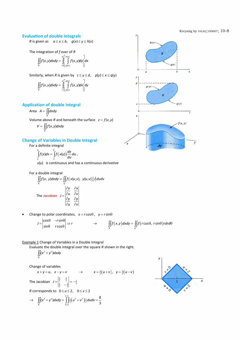
Kreyszig by YHLEE;100607; 10-8 Evaluation of double integrals R is given as , ( ) ( )a x b g x y h x≤ ≤ ≤ ≤
The integration of f over of R
( )
( )
( , ) ( , )h xb
R a g x
f x y dxdy f x y dy dx⎡ ⎤
= ⎢ ⎥⎢ ⎥⎣ ⎦
∫∫ ∫ ∫
Similarly, when R is given by , ( ) ( )c y d p y x q y≤ ≤ ≤ ≤
( )
( )
( , ) ( , )q yd
R c p y
f x y dxdy f x y dx dy⎡ ⎤
= ⎢ ⎥⎢ ⎥⎣ ⎦
∫∫ ∫ ∫
Application of double integral Area
R
A dxdy= ∫∫
Volume above R and beneath the surface ( , )z f x y=
( , )R
V f x y dxdy= ∫∫
Change of Variables in Double Integral For a definite integral
( )( ) ( )b
a
dxf x dx f x u du
du
β
α
=∫ ∫ ,
( )x u is continuous and has a continuous derivative For a double integral
( )( , ) ( , ), ( , )R R
f x y dxdy f x u v y u v J dudv=∫∫ ∫∫
The Jacobian
x xu vJy yu v
∂ ∂∂ ∂=∂ ∂∂ ∂
• Change to polar coordinates, cos , sinx r y r= θ = θ
cos sin
sin cos
rJ r
r
θ − θ= ⇒
θ θ → ( ) ( )
*
, cos , sinR R
f x y dxdy f r r rdrd= θ θ θ∫∫ ∫∫
Example 1 Change of Variables in a Double Integral Evaluate the double integral over the square R shown in the right.
2 2( )R
x y dxdy+∫∫
Change of variables , x y u x y v+ = − = → ( ) ( )1 1
2 2, x u v y u v= + = −
The Jacobian 1 12 2 1
21 12 2
J = = −−
R corresponds to 0 2, 0 2u v≤ ≤ ≤ ≤
→ ( )2 2
2 2 2 21 12 2
0 0
8( )
3R
x y dxdy u v dudv+ = + =∫∫ ∫ ∫

Kreyszig by YHLEE;100607; 10-9 10.4 Green's Theorem in the plane Theorem 1 Green's theorem in the plane (Transformation between Double Integrals and Line Integrals)
R : closed bounded region in xy‐plane C : boundary of R Then
( )2 11 2c
R
F Fdxdy F dx F dy
x y
∂ ∂⎛ ⎞− = +⎜ ⎟∂ ∂⎝ ⎠
∫∫ ∫
In vectorial form
( ) ˆ R C
F k dxdy F dr∇× • = •∫∫ ∫
(Right hand rule between k̂ and C ) Proof : The region R is given as , ( ) ( )a x b u x y v x≤ ≤ ≤ ≤ or , ( ) ( )c y d p y x q y≤ ≤ ≤ ≤
The second integral on the left side
( ) ( )( )
1 11 1
( )
, ( ) , ( )v xb b
R a u x a
F Fdxdy dy dx F x v x F x u x dx
y y
⎡ ⎤∂ ∂⇒ ⇒ −⎡ ⎤⎢ ⎥ ⎣ ⎦∂ ∂⎢ ⎥⎣ ⎦
∫∫ ∫ ∫ ∫ ( ) ( )1 1, ( ) , ( )b a
a b
F x u x dx F x v x dx⇒ − −∫ ∫
* **
1 1( , ) ( , )C C
F x y dx F x y dx⇒− −∫ ∫ 1( , )C
F x y dx⇒−∫ ↑ reversed range
The first integral
( ) ( )( )
2 22 2
( )
( ), ( ),q yd d c
R c p y c d
F Fdxdy dx dy F q y y dy F p y y dy
x x
⎡ ⎤∂ ∂⇒ ⇒ +⎢ ⎥
∂ ∂⎢ ⎥⎣ ⎦∫∫ ∫ ∫ ∫ ∫ 2 ( , )
C
F x y dy⇒ ∫
↑ reversed range By combining
( )2 11 2
R C
F Fdxdy F dx F dy
x y
∂ ∂⎛ ⎞− ⇒ +⎜ ⎟∂ ∂⎝ ⎠
∫∫ ∫
• In general R can be subdivided
Kreyszig by YHLEE;100607; 10-10 Example 1 2
1 7F y y= − , 2 2 2F xy x= + C : a circle 2 2 1x y+ =
Then
( ) ( )2 1 2 2 2 7 9 9R R R
F Fdxdy y y dxdy dxdy
x y
∂ ∂⎛ ⎞− ⇒ + − − ⇒ ⇒ π⎡ ⎤⎜ ⎟ ⎣ ⎦∂ ∂⎝ ⎠
∫∫ ∫∫ ∫∫
The curve is represented
ˆ ˆ( ) cos sin r t t i t j= + 0 2t≤ ≤ π
ˆ ˆ( ) sin cos r t t i t j′ = − + On C 2
1 sin 7sinF t t= − , 2 2cos sin 2cosF t t t= +
( )( ) ( )2
2
0
' sin 7sin sin 2cos sin 2cos cosC C
F dr F r dt t t t t t t t dtπ
⎡ ⎤• = • ⇒ − − + +⎣ ⎦∫ ∫ ∫ ⇒9π
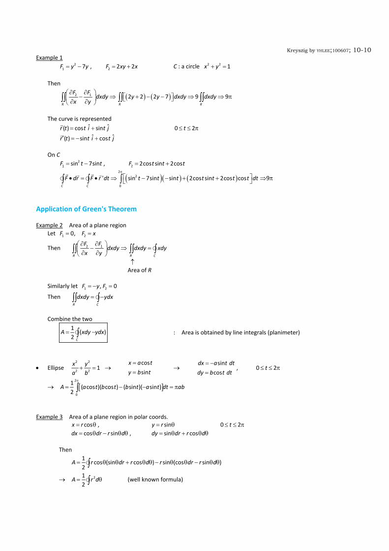
Application of Green's Theorem Example 2 Area of a plane region Let 1 20, F F x= =
Then 2 1
R R C
F Fdxdy dxdy xdy
x y
∂ ∂⎛ ⎞− ⇒ =⎜ ⎟∂ ∂⎝ ⎠∫∫ ∫∫ ∫
↑ Area of R Similarly let 1 2, 0F y F= − =
Then R C
dxdy ydx= −∫∫ ∫
Combine the two
1
( )2 C
A xdy ydx= −∫ : Area is obtained by line integrals (planimeter)
• Ellipse 2 2
2 21
x ya b
+ = → cos
sin
x a t
y b t
==
→ sin
cos
dx a t dt
dy b t dt
= −=
, 0 2t≤ ≤ π
→ [ ]2
0
1( cos )( cos ) ( sin )( sin )
2A a t b t b t a t dt ab
π
= − − = π∫
Example 3 Area of a plane region in polar coords. cosx r= θ , siny r= θ 0 2t≤ ≤ π cos sindx dr r d= θ − θ θ , sin cosdy dr r d= θ + θ θ Then
1
cos (sin cos ) sin (cos sin )2
A r dr r d r dr r d= θ θ + θ θ − θ θ − θ θ∫
→ 212
A r d= θ∫ (well known formula)

Kreyszig by YHLEE;100607; 10-11 Example 4 Transformation of a double integral of the Laplacian into a line integral
Let w(x,y) be defined in R in xy plane and ( )F wk≡∇× −
ˆ( )R C
F kdxdy F dr∇× • = •∫∫ ∫
→ 2 ˆ ˆ ˆ( ) ( )R C
drwk kdxdy wk ds
ds∇ • = ∇× − •∫∫ ∫
↑ ↑ 2
0
ˆ ˆ ˆ( ) ( ) ( )F wk wk wk⇒
∇× =∇×∇× − ⇒∇∇• − −∇ − ,
From ( )u v v u u v∇• × = •∇× − •∇×
⇒ ˆ ˆ( ) ( )dr dr
wk wkds ds
⎡ ⎤ ⎡ ⎤∇ • − × + ∇× • −⎢ ⎥ ⎢ ⎥⎣ ⎦ ⎣ ⎦
⇒ ˆ ˆdr drw k w k
ds ds⎡ ⎤ ⎡ ⎤∇ • − × + ∇• − ×⎢ ⎥ ⎢ ⎥⎣ ⎦ ⎣ ⎦
+0
ˆ ˆ( ) ( )dr dr
w k kds ds
⇒
⎡ ⎤⎛ ⎞∇• × − +∇× − •⎢ ⎥⎜ ⎟⎝ ⎠⎢ ⎥⎣ ⎦
⇒ ˆ drw k
ds⎡ ⎤∇ • − ×⎢ ⎥⎣ ⎦
↑ = n̂ Therefore
2 ˆ R C
w dxdy w n ds∇ = ∇ •∫∫ ∫
n̂ , outer unit normal to C
10.5 Surfaces for Surface Integrals Representations of surfaces In xyz‐space ( , ) or ( , , ) 0z f x y g x y z= =
• Parametric representation
ˆˆ ˆ( , ) ( , ) ( , ) ( , )r u v x u v i y u v j z u v k= + + , : ( , ) in u v R

Kreyszig by YHLEE;100607; 10-12 Example 1 Parametric Representation of a Cylinder 2 2 2 , 1 1x y a z+ = − ≤ ≤
Parametric representation
ˆˆ ˆ( , ) cos sin r u v a u i a u j vk= + + where 0 2u≤ ≤ π , 1 1v− ≤ ≤ Example 2 Parametric Representation of a Sphere 2 2 2 2x y z a+ + = Parametric representation (different from spherical coordinates.)
ˆˆ ˆ( , ) cos cos cos sin sin r u v a v u i a v u j a v k= + +
where 0 2u≤ ≤ π for meridian, 2 2
vπ π
− ≤ ≤ for parallel
Example 3 Parametric Representation of a Cone
2 2 , 0z x y z H= + ≤ ≤
ˆˆ ˆ( , ) cos sin r u v u v i u v j u k= + + , where 0 , 0 2u H v≤ ≤ ≤ ≤ π
Tangent Plane and Surface Normal Tangent plane of S at P : Plane containing tangent vectors of S at P Normal vector of S at P : A vector perpendicular to the tangent plane • Parametric representation of S : ( , )r u v
A curve C on S : ( ) 1( ), ( ) ( )r u t v t r t≡
A tangent vector of C : 11 ( )
dr r rr t u v
dt u v∂ ∂′ ′ ′= ⇒ +∂ ∂
↑ ↑ Tangent vectors of S at P
A normal vector of S at P : u v
r rN r r
u v∂ ∂
= × ≡ ×∂ ∂
The unit normal vector : ˆ Nn
N=
• When S is given by ( , , ) 0g x y z =
The surface normal vector : N g=∇

Kreyszig by YHLEE;100607; 10-13 Example 4 Unit Normal Vector of a Sphere 2 2 2 2( , , ) 0g x y z x y z a= + + − =
→ ˆˆ ˆgrad 2 2 2g xi yj zk= + +
→ ˆˆ ˆˆ x y zn i j k
a a a= + +
Example 5 Unit Normal Vector of a Cone
( ) 2 2, ,g x y z z x y= − + +
→ 2 2 2 2
ˆˆ ˆx yg i j k
x y x y∇ = + −
+ +
→ 2 2 2 2
1 ˆˆ ˆˆ2
x yn i j k
x y x y
⎛ ⎞⎜ ⎟= + −⎜ ⎟+ +⎝ ⎠
10.6 Surface Integrals A surface S in parametric representation : ˆˆ ˆ( , ) ( , ) ( , ) ( , )r u v x u v i y u v j z u v k= + +
The surface normal vector : u v
r rN r r
u v∂ ∂
= × ≡ ×∂ ∂
, 1
n̂ NN
=
The element of area of S : ˆ ˆ ˆu v u vNdudv n r r dudv n r du r dv ndA⇒ × ⇒ × ⇒
A surface integral of ( )F r over S
ˆS S R
F dA F ndA F N dudv• ≡ • = •∫∫ ∫∫ ∫∫
If (Volume density of fluid Velocity)F v= ρ × → The integral gives the flux across S
↑ (Mass crossing S per unit time) Flux density(Mass per unit time per unit area) • The surface integral in component form Using [ ]1 2 3, ,F F F F= , [ ]1 2 3, ,N N N N= and [ ]ˆ cos , cos , cosn = α β γ
( )
( )
( )
1 2 3
1 2 3
1 1 2 2 3 3
cos cos cos
S S
S
R
F dA F F F dA
F dydz F dzdx F dxdy
F N F N F N dudv
• = α + β+ γ
= + +
= + +
∫∫ ∫∫
∫∫
∫∫
Note cos , cos , cosdA dydz dA dzdx dA dxdyα = β = γ =

Kreyszig by YHLEE;100607; 10-14 Example 1 Flux through a Surface Find the flux of water through 2 : , 0 2, 0 3S y x x z= ≤ ≤ ≤ ≤
The water velocity 2 ˆˆ ˆ3 6 6F z i j xzk= + + [m/sec]
Let 2, ,x u z v y u= = =
The surface S
2 ˆˆ ˆr ui u j vk= + + → ˆ ˆ2ur i uj= + , ˆvr k=
ˆ ˆ2u vN r r ui j= × ⇒ −
On S
2 ˆˆ ˆ 3 6 6F v i j uvk= + + → 26 6F N uv• = − The surface integral
( ) ( )3 2 3 3
32 2 2 2 3
00 0 0 0
(6 6) 3 6 12 12 72[ / ]u
R
F Ndudv uv dudv u v u dv v dv m s=
• ⇒ − ⇒ − ⇒ − ⇒∫∫ ∫ ∫ ∫ ∫
• Check
ˆ ˆ ˆ ˆ2 2N ui j x i j= − ⇒ − → cos 0, cos 0 cos , not presentα > β < γ
( )3 4 2 3
21 2 3
0 0 0 0
3 6 72S
F dydz F dzdx F dxdy z dydz dzdx+ + ⇒ − ⇒∫∫ ∫ ∫ ∫ ∫
↑ Minus sign because cos 0β <
Example 2 Surface Integral
Find the surface integral of 2 2 ˆˆ 3F x i y k= + over S: x+y+z=1 in the first octant. Solution : Let , , then 1x u y v z u v= = = − −
The surface S
ˆˆ ˆ( , ) (1 )r u v ui vj u v k= + + − − → ˆˆ ˆu vN r r i j k= × ⇒ + +
On S
2 2 ˆˆ 3F u i v k= + → 2 23F N u v• = + Then
( ) ( )1 1 1
32 2 2 2 2
0 0 0
1 1( 3 ) ( 3 ) 1 3 1
3 3
v
R R
F N dudv u v dudv u v dudv v v v dv− ⎡ ⎤• ⇒ + ⇒ + ⇒ − + − ⇒⎢ ⎥⎣ ⎦∫∫ ∫∫ ∫ ∫ ∫

Kreyszig by YHLEE;100607; 10-15 Orientation of Surfaces Theorem 1 Change of Orientation in a Surface Integral
If n̂ is replaced by n̂− , the surface integral is multiplied by ‐1 N is reversed if u and v are interchanged. v u u vr r r r N× = − × ⇒ −
Orientation of Smooth Surfaces A surface S is orientable if its normal direction can be defined uniquely and continuously over S. Then, the normal direction is associated with the direction of the boundary C. (Right hand rule) The piecewise smooth surface is orientable if the direction of *C for 1S is opposite to that for 2S .
Nonorientable surface
Surface Integrals Without Regard to Orientation
( ) ( )( ) ( ) , ,S R
G r dA G r u v N u v dudv⇒∫∫ ∫∫
↑ u vdA N dudv r r dudv= = × in
R
F N dudv•∫∫
• Area of S
u vS R
A dA r r dudv= = ×∫∫ ∫∫

Kreyszig by YHLEE;100607; 10-16 • When a surface S is given by z=f(x,y) We let x=u, y=v.
→ ˆˆ ˆ( , ) ( , )r u v ui v j f u v k= + +
→ ˆˆ ˆu v u vN r r f i f j k= × ⇒ − − + , 2 21 u vN f f= + +
( )*
22
( ) , , ( , ) 1S R
f fG r dA G x y f x y dxdy
x y∂ ∂⎛ ⎞⎛ ⎞= + + ⎜ ⎟⎜ ⎟∂ ∂⎝ ⎠ ⎝ ⎠
∫∫ ∫∫
where *R : projection of S on xy plane Area of S in this case
*
22
1R
f fA dxdy
x y∂ ∂⎛ ⎞⎛ ⎞= + + ⎜ ⎟⎜ ⎟∂ ∂⎝ ⎠ ⎝ ⎠∫∫
Example 4 Area of a Sphere A sphere with radius a
ˆˆ ˆ( , ) cos cos cos sin sin r u v a v u i a v u j a v k= + + where 0 2 , / 2 / 2u v≤ ≤ π − π ≤ ≤ π
Find
2 2 2 2 2cos cos , cos sin , cos cosu vr r a v u a v u a v u⎡ ⎤× = ⎣ ⎦
r r a vu v× = 2 cos
Then
/2 2
2 2
/2 0
cos 4A a v dudv aπ π
−π
= = π∫ ∫
10.7 Triple Integrals. Divergence Theorem of Gauss A triple integral of f over region T
( )0
1
lim , , ( , , )n
k k k kDk T
f x y z V f x y z dxdydz→
=
Δ ≡∑ ∫∫∫ or ( , , )T
f x y z dV∫∫∫
↑ ↑ ↑ Max. diagonal of cubes A point in the k‐th cube Volume of the k‐th cube Divergence Theorem of Gauss Triple integral ↔ Closed surface integral

Kreyszig by YHLEE;100607; 10-17 Theorem 1 Divergence Theorem of Gauss (Transformation between Triple and Surface Integrals)
T is a bounded region whose boundary is a piecewise smooth orientable surface S. ( , , )F x y z is continuous and has continuous first part derivative in T.
Then
T S
F dV F dA∇• = •∫∫∫ ∫∫
ˆdA ndA= , n̂ is the outer unit surface normal vector
→ 31 21 2 3( cos cos cos )
T S
FF Fdxdydz F F F dA
x y z
∂∂ ∂⎛ ⎞+ + = α + β+ γ⎜ ⎟∂ ∂ ∂⎝ ⎠
∫∫∫ ∫∫
= 1 2 3R
F dydz F dzdx F dxdy+ +∫∫
where 1 2 3ˆˆ ˆF F i F j F k= + + ,
ˆˆ ˆˆ cos cos cos n i j k= α + β + γ
Prove term by term .
First, consider 33 cos
T S
Fdxdydz F dA
dz
∂= γ∫∫∫ ∫∫ .
1S : Upper surface, z = h(x,y).
2S : Lower surface, z= g(x,y).
3S : Side surface.
Then, the left term
[ ]( , )
3 33 3
( , )
( , , ( , )) ( , , ( , ))h x y
T R g x y R
F Fdxdydz dz dxdy F x y h x y F x y g x y dxdy
z z
⎡ ⎤∂ ∂⇒ ⇒ −⎢ ⎥
∂ ∂⎢ ⎥⎣ ⎦∫∫∫ ∫∫ ∫ ∫∫
The right term
1 2
3 3 3 3cos ( , , ( , )) ( , , ( , ))S S S R R
F dA F dxdy F x y h x y dxdy F x y g x y dxdy+
γ ⇒ ⇒ −∫∫ ∫∫ ∫∫ ∫∫
↑ ↑ Minus sign because cos 0γ <
dxdy is the projection of dA onto xy‐plane Similarly, one can prove the other terms. Example 2 Verification of the Divergence Theorem Evaluate the integral over the sphere 2 2 2: 4S x y z+ + =
( )ˆˆ7S
x i z k dA− •∫∫
(a) Using Divergence theorem
( )34 2ˆˆ ˆ7 6
3S T
x i z k n dA F dVπ
− • = ∇• ⇒ ⋅∫∫ ∫∫∫
↑ 7 1 6F∇• = − =

Kreyszig by YHLEE;100607; 10-18
(b) Direct calculation
Using 2cos sin , 2sinx v u z u= = , the vector function is
The surface integral
( )/2 2
3 2 2
/2 0
56cos cos 8cos sinv u
v u v v dudvπ π
=−π =
−∫ ∫
Coordinate Invariance of the Divergence Mean value theorem for triple integrals
( ) ( ) ( ), , , ,o o o oT
f x y z dV f x y z V T=∫∫∫
↑ ↑ Volume of T. A point in T. Apply this to the Divergence theorem
div T S
F dV F dA= •∫∫∫ ∫∫ → ( ) ( ) ( )
1div , ,o o o
S T
F x y z F dAV T
= •∫∫
↑ ( ) ( )div , ,o o oF x y z V T
Let T shrink down to P.
( ) ( )0
1div lim
TS
F P F dAV T→
= •∫∫
Theorem 2 Invariance of the Divergence
Divergnece of F with continuous first partial derivatives is independent of the particular choice of Cartesian coordinates.
10.8 Further Applications of the Divergence Theorem Potential Theory. Harmonic Functions
Solving the Laplace equation 2 2 2
22 2 2
0f f f
fx y z∂ ∂ ∂
∇ = + + =∂ ∂ ∂
: Potential theory
Its solution with continuous second‐order partial derivatives :Harmonic function

Kreyszig by YHLEE;100607; 10-19 Example 1 A Basic Property of Solution of Laplace’s equation From divergence theorem
ˆ T S
F dV F ndA∇• = •∫∫∫ ∫∫
Let gradF f=
→ 2( )F f f∇• ⇒∇• ∇ ⇒∇
ˆ ˆF n f n• ⇒∇ •
→ 2 T S
ff dV dA
n∂
∇ =∂∫∫∫ ∫∫
Example 5 Green's Theorem Let F f g= ∇
→ 2( )F f g f g f g∇• ⇒∇• ∇ ⇒ ∇ +∇ •∇
ˆ ˆ ˆ( ) ( )g
F n f g n f n g fn∂
• ⇒ ∇ • ⇒ •∇ ⇒∂
From ˆ T S
F dV F n dA∇• = •∫∫∫ ∫∫
→ 2( )T S
gf g f g dV f dA
n∂
∇ +∇ •∇ =∂∫∫∫ ∫∫ : Green's first formula
Let F g f= ∇ , and obtain the similar equation. From the difference of the two
2 2( ) ( )T S
g ff g g f dV f g dA
n n∂ ∂
∇ − ∇ = −∂ ∂∫∫∫ ∫∫ : Green's second formula
Theorem 2 Harmonic Functions
Let ( ), ,f x y z be harmonic and zero at every point on a closed surface S,
Then f is identically zero in the region enclosed by S. Theorem 3 Uniqueness Theorem for Laplace’s Equation
A harmonic function f(x,y,z) is uniquely determined in the inside of T by its values on the enclosing surface S.
Proof: Let 1 2 and f f be harmonic functions with the same boundary condition on S.
Let 1 2g f f= −
→ 0g = on S Then, from theorem 2, → 1 2 0g f f= − =

Kreyszig by YHLEE;100607; 10-20
10.9 Stokes's Theorem Theorem 1 Stokes’s Theorem (Transformation between Surface and Line Integrals)
Let S be a piecewise smooth oriented surface whose boundary is a piecewise smooth simple closed curve C. Let ( , , )F x y z be a continuous vector function with continuous first partial derivatives.
( )S C
F dA F dr∇× • = •∫∫ ∫
( )ˆ , 'dA n dA dr r s ds= =
Using n̂dA Ndudv=
3 32 1 2 11 2 3
R
F FF F F FN N N dudv
y z z x x y
⎡ ⎤∂ ∂∂ ∂ ∂ ∂⎛ ⎞ ⎛ ⎞⎛ ⎞− + − + −⎢ ⎥⎜ ⎟ ⎜ ⎟⎜ ⎟∂ ∂ ∂ ∂ ∂ ∂⎝ ⎠⎝ ⎠ ⎝ ⎠⎣ ⎦∫∫
( )1 2 3C
F dx F dy F dz= + +∫
Proof: Prove the theorem term by term
1 12 3 1
R C
F FN N dudv F dx
z y
∂ ∂⎛ ⎞− =⎜ ⎟∂ ∂⎝ ⎠
∫∫ ∫ , 2 21 3 2
R C
F FN N dudv F dy
z x
∂ ∂⎛ ⎞− + =⎜ ⎟∂ ∂⎝ ⎠∫∫ ∫ , 3 31 2 3
R C
F FN N dudv F dz
y x
∂ ∂⎛ ⎞− =⎜ ⎟∂ ∂⎝ ⎠
∫∫ ∫
Consider the first term
1 12 3 1
R C
F FN N dudv F dx
z y
∂ ∂⎛ ⎞− =⎜ ⎟∂ ∂⎝ ⎠
∫∫ ∫
The surface S can be given by ( ),z f x y= , ( ),y g x z= , or ( ),x h y z=
Let u=x, v=y for a parametric representation of S
→ ( ) ˆˆ ˆ( , ) ,r x y x i y j f x y k= + +
ˆˆ ˆ
ˆˆ ˆ1 0 /
0 1 /x y x y
i j k
N r r f x f i f j k
f y
= × ⇒ ∂ ∂ ⇒ − − +∂ ∂
,
Projection of S onto xy plane → * * with boundary S C Then, the left term
*
1 1( )yS
F Ff dxdy
z y
∂ ∂⎡ ⎤− −⎢ ⎥∂ ∂⎣ ⎦∫∫
The right term
* *
11
C S
FF dx dxdy
y
∂⇒ −
∂∫ ∫∫*
1 1( , , ) ( , , )
S
F x y f F x y f fdxdy
y f y
∂ ∂ ∂⎡ ⎤⇒ − −⎢ ⎥∂ ∂ ∂⎣ ⎦∫∫ , where ( , )z f x y=
↑
From the Green's theorem, ( )2 11 2c
R
F Fdxdy F dx F dy
x y
∂ ∂⎛ ⎞− = +⎜ ⎟∂ ∂⎝ ⎠∫∫ ∫

Kreyszig by YHLEE;100607; 10-21 Example 1 Verification of Stokes’s Theorem
Let [ ], , F y z x= and S is the paraboloid, ( ) ( )2 2, 1z f x y x y= = − + for 0z ≥ .
The curve ( ) [ ]cos , sin , 0r s s s=
→ ( ) [ ]' sin , cos , 0r s s s= −
On the curve [ ] [ ], , sin , 0, cosF y z x s s= =
Hence
( )( ) ( ) ( )( )2 2
0 0
' sin sin 0 0C
F dr F r s r s ds s s dsπ π
• ⇒ • ⇒ − + + = −π⎡ ⎤⎣ ⎦∫ ∫ ∫
• The surface integral
ˆˆ ˆ
ˆˆ ˆ
i j k
F x i j kx y zy z x
∂ ∂ ∂∇× = ⇒ − − −
∂ ∂ ∂
( ) ˆˆ ˆ( , ) ,r x y x i y j f x y k= + +
ˆˆ ˆ
ˆˆ ˆ1 0 /
0 1 /x y x y
i j k
N r r f x f i f j k
f y
= × ⇒ ∂ ∂ ⇒ − − +∂ ∂
⇒ + + ˆˆ ˆ2 2x i y j k
( ) ( ) ( ) ( )2 1
0 0
2 2 1 2 cos sin 1S R R r
F dA F N dxdy x y dxdy r rdrdπ
θ= =
∇× • = ∇× • ⇒ − − − ⇒ − θ+ θ − θ = −π⎡ ⎤⎣ ⎦∫∫ ∫∫ ∫∫ ∫ ∫
↑ In cylindrical coordinates Example 4 Physical Meaning of the Curl in Fluid Motion. Circulation Let
orS be a circular disk of radius or centered at P with boundary
orC
Let ( , , )F x y z be a vector function Then
( ) *at ˆ ˆ( )
o
r ro o
rPC S
F dr F ndA F n A• = ∇× • ⇒ ∇× •∫ ∫∫
↑ ↑ ↑ ↑ Area of or
S
Stokes's theorem A point in or
S
Mean value theorem,
→ ( ) *at
1ˆo ro
Pr C
F n F drA
∇× • = •∫
↑

Kreyszig by YHLEE;100607; 10-22 Circulation of F around
orC
→ ( )at 0
1ˆ limr
P rr C
F n F drA→
∇× • = •∫
Therefore
Circulation of in the plane perpendicular to
curl in direction = Area enclosed by the curve
FF
ξξ
Stokes's theorem Applied to Path Independence
If the line integral C
F dr•∫ is independent of path, then curl 0F = (proved in the previous section)
If curl 0F = , then C
F dr•∫ is independent of path.
It can be proved using Stokes's theorem.
→ ( ) 0C S
F dr F dA• = ∇× • ⇒∫ ∫∫ ,
↑ Because 0F∇× = Since the closed line integral of F is always zero regardless of C,
the line integral C
F dr•∫ is independent of path.