Evaluation of Instream Flow Needs in the Lower Klamath River
247
Evaluation of Instream Flow Needs in the Lower Klamath River Phase II Final Report Prepared for: U.S. Department of the Interior Prepared by: Dr. Thomas B. Hardy Dr. R. Craig Addley Dr. Ekaterina Saraeva Institute for Natural Systems Engineering Utah Water Research Laboratory Utah State University Logan, Utah 84322-4110 July 31, 2006
-
Upload
nguyenduong -
Category
Documents
-
view
215 -
download
1
Transcript of Evaluation of Instream Flow Needs in the Lower Klamath River

Evaluation of Instream Flow Needs in the Lower Klamath River
Phase II
Final Report
Prepared for:
U.S. Department of the Interior
Prepared by:
Dr. Thomas B. Hardy Dr. R. Craig Addley
Dr. Ekaterina Saraeva Institute for Natural Systems Engineering
Utah Water Research Laboratory Utah State University
Logan, Utah 84322-4110
July 31, 2006

i
This report is dedicated to the memory of
Ronnie Pierce (1942 – 2005)
She held everyone accountable to the truth, their actions, and attitudes without regard to race, color, creed, political position, or
affiliation on any issue dealing with salmon in the Klamath Basin. We can all learn from her unwavering dedication to salmon restoration.

ii
Acknowledgements The completion of this work in large part can be attributed to the efforts of the U.S. Fish and Wildlife Service Arcata Field Office staff and in particular to Mr. Thomas Shaw for providing much of the supporting site-specific field data, habitat mapping, and fisheries data used in the analyses. The efforts of the various Tribal fisheries personnel were critical in supplying additional fisheries collection data, and intensive site substrate and cover mapping; in particular, the efforts of Tim Hayden, Charlie Chamberlain and Mike Belchik. USGS personnel from the Midcontinent Ecological Science Center provided valuable assistance. Mr. Gary Smith and Mike Rode of the California Department of Fish and Game also provided critical information on site-specific habitat suitability criteria and conceptual foundations for the escape cover analysis used in the habitat simulations. Much of this later work was supported by work of Tim Harden (Harden and Associates). The Bureau of Reclamation also provided valuable input during the Phase II study process on Klamath Project operations. Special thanks to Mr. Mike Deas (Water Course Engineering, Inc.) for providing water temperature simulations below Iron Gate Dam. The Technical Team also provided critical input and review of all technical elements of this work as well as providing reviews of the report. Finally, the completion of this work would not have been possible without the tireless efforts of Jennifer Ludlow, Mark Winkelaar, James Shoemaker, Shannon Clemens, Jerilyn Brunson, William Bradford, Sarah Blake, Brandy Blank, Matt Combes, Leon Basdekas, Lisa Kent, Carri Richards, and Aaron Hardy at the Institute for Natural Systems Engineering, Utah State University.
Purpose of the Report The purpose of this report is to recommend instream flows on a monthly basis for specific reaches of the main stem Klamath River below Iron Gate Dam by different water year types. These recommendations specify flow regimes that will provide for the long-term protection, enhancement, and recovery of the aquatic resources within the main stem Klamath River in light of the Department of the Interior’s trust responsibility to protect tribal rights and resources as well as other statutory responsibilities, such as the Endangered Species Act. The recommendations are made in consideration of all the anadromous species and life stages on a seasonal basis and do not focus on specific target species or life stages (i.e., coho).

iii
Executive Summary This report details the analytical approach and modeling results from site-specific studies conducted within the main stem Klamath River below Iron Gate Dam downstream to the estuary. Study results are utilized to make revised interim instream flow recommendations necessary to protect the aquatic resources within the main stem Klamath River between Iron Gate and the estuary. This report was developed for the Department of the Interior (DOI) who provided access to a technical review team composed of representatives of the U.S. Fish and Wildlife Service, Bureau of Reclamation, Bureau of Indian Affairs, U.S. Geological Survey, and the National Marine Fisheries Service. The technical review team also included participation by the Yurok, Hoopa Valley, and Karuk Tribes given the Departments trust responsibilities and the California Department of Fish and Game as the state level resource management agency. Subsequent to the initial draft, participation included representatives from the Oregon Department of Fish and Wildlife, PacifiCorp, and consultants to the Klamath Water User Association. The technical team provided invaluable assistance in the review of methods and results used in the analysis, provided data and supporting material for use in completion of the Phase II report, and valuable comments/suggestions on the draft report. In addition, several agencies and private individuals provided written comments on the Draft Report, which have been addressed in this report where appropriate. This report is organized to follow the general process used to implement the technical studies. It first provides important background information on the historical and current conditions of the anadromous species, highlights factors that have contributed to their decline, and provides an overview of the Phase II technical study process. Key sections address methods and findings for each technical component such as study design, study site selection, field methods, analytical approaches, modeling approaches, summary results, recommended instream flows, and justifications/rationale for these recommendations. The Phase II study relied on state-of-the-art field data collection methodologies and modeling of physical habitat for target species and life stages of anadromous fish. We also relied on bioenergetic based modeling of growth and salmon production estimates to evaluate our recommendations in light of existing conditions. Physical habitat modeling for target species and life stages of anadromous fish were validated against empirical fish observations from the main stem Klamath River. Temperature simulations were utilized to examine thermal niche implications of the flow regime on rearing, upstream migration, outmigration, and disease factors. These results were also related to behavioral thermoregulation by salmon. The integration of the habitat modeling with the unimpaired hydrology was used from the perspective of the Natural Flow Paradigm to develop recommendations for flow regimes that mimic the expected characteristics of the natural flow regime. This was approached by linking target instream flow regimes on a monthly basis to the annual inflow exceedence levels for net Upper Klamath inflows.
iv
The flow recommendation process considered all species and life stages present in a given month when defining flow needs. In general, the methodology strived to maintain habitat and flow conditions to within the expected monthly variation based on the use of stochastic time series of monthly flows generated from the Bureau of Reclamation’s Natural Flow Study. The flow recommendations developed in the Iron Gate to Shasta River reach were ‘propagated’ downstream to each study site by addition of reach gains and evaluated based on modeled conditions derived from site-specific data in each reach. Flow recommendations are provided for the following components of the flow regime based on NRC (2005), but also address ramping rates and fish disease issues:
• Over Bank Flows • High Flow Pulses • Base Flows • Subsistence Flows • Ecological Base Flows
v
Table of Contents Acknowledgements ..........................................................................................................ii Purpose of the Report ......................................................................................................ii Executive Summary ........................................................................................................ iii Table of Contents............................................................................................................ v List of Figures................................................................................................................ viii List of Tables.................................................................................................................xvi Introduction ..................................................................................................................... 1 Background ..................................................................................................................... 2 Overview of Fisheries Resources.................................................................................... 3
Historical Distribution ................................................................................................... 3 Steelhead (Oncorhynchus mykiss)........................................................................... 3 Coho Salmon (Oncorhynchus kisutch)..................................................................... 4 Chinook Salmon (Oncorhynchus tshawytscha)........................................................ 4 Green and White Sturgeon (Acipenser medirostris and A. transmontanus)............. 4 Coastal Cutthroat Trout (Oncorhynchus clarki clarki)............................................... 5 Eulachon (Candlefish) (Thaleichthys pacificus) ....................................................... 5 Pacific Lamprey (Lampetra tridentata) ..................................................................... 5
Current Distribution...................................................................................................... 5 Overall Population Trends in Anadromous Species..................................................... 6
Steelhead................................................................................................................. 6 Coho ........................................................................................................................ 6 Chinook.................................................................................................................... 7
Factors Attributed to the Decline of Anadromous Species........................................... 7 Basin Wide Overview ............................................................................................... 7 The Upper Klamath Basin ...................................................................................... 10 The Shasta Subbasin............................................................................................. 11 The Scott Subbasin................................................................................................ 12 The Salmon Subbasin............................................................................................ 13 The Mid-Klamath Subbasin.................................................................................... 14 The Trinity Subbasin .............................................................................................. 15 The Lower Klamath Subbasin ................................................................................ 19
Life History Traits....................................................................................................... 20 Steelhead............................................................................................................... 20 Coho Salmon ......................................................................................................... 21 Chinook Salmon..................................................................................................... 21 Green Sturgeon...................................................................................................... 22 Coastal Cutthroat Trout.......................................................................................... 23 Eulachon (Candlefish)............................................................................................ 23 Pacific Lamprey...................................................................................................... 23
Hydrology ...................................................................................................................... 23 Assessment of Hydrologic Alterations ....................................................................... 24
Empirical Based Estimates of the Main Stem Klamath River Historical Flows at Keno and Iron Gate................................................................................................ 24

vi
Seasonal Changes in the Main Stem Klamath River Hydrology at Keno and Iron Gate ....................................................................................................................... 26 Klamath Project Operations and Flows downstream of Iron Gate Dam ................. 27
Simulated Unimpaired and Natural Flows in the main stem Klamath River ............... 31 Upper Klamath Lake Level Pool-Consumptive Use Based Estimated Unimpaired Hydrology............................................................................................ 32 BOR Natural Flow Study Hydrology ....................................................................... 33 Estimation of Unimpaired Accretions ..................................................................... 33 Comparison of Estimated Hydrology...................................................................... 34
Water Quality and Temperature Evaluations................................................................. 37 Water Quality/Temperature Modeling ........................................................................ 38
SIAM-MODSIM/HEC-5Q........................................................................................ 38 RMA-2/11............................................................................................................... 39 Relationship between Flow Model Computational Nodes and USU Study Sites.... 40
Comparison of Estimated Thermal Regimes ............................................................. 40 Assessment of Water Quality and Thermal Alterations.............................................. 43
Geomorphic and Riparian Evaluations .......................................................................... 48 Phase II Integrated Assessment Framework................................................................. 49 Phase II General Process ............................................................................................. 50
Study Design ............................................................................................................. 51 River Reach Stratification .......................................................................................... 52 Overview of Study Site Selection............................................................................... 53
Habitat Mapping ..................................................................................................... 54 Selection of USU Study Sites................................................................................. 57
Channel Characterization .......................................................................................... 58 USU Field Methodologies for Channel Characterization ........................................ 58 Water Surface Elevation and Water Velocity Mapping........................................... 72 Substrate and Vegetation Mapping ........................................................................ 73
Stochastic Time Series Modeling for Flows ............................................................... 80 Hydraulic Modeling .................................................................................................... 86
Development of Computational Meshes ................................................................ 86 Water Surface Modeling......................................................................................... 87 Velocity Modeling ................................................................................................... 91 Ranges of Simulated Flows ................................................................................... 93
Fish Habitat Utilization ............................................................................................... 93 Selection of Target Species and Life Stages for Phase II Evaluations ...................... 94 Species and Life Stage Periodicities.......................................................................... 95
Monthly Species and Life Stage Critical Factors Related to Flows ........................ 95 The Ecological Basis of Habitat Suitability Criteria (i.e. Niche Theory) ...................... 98 Development of Site Specific HSC .......................................................................... 101
Substrate and Vegetation Coding for HSC........................................................... 101 Chinook Spawning ............................................................................................... 101 Chinook Fry.......................................................................................................... 104 Chinook Juvenile.................................................................................................. 107 Steelhead 1+ (Juveniles) ...................................................................................... 110 Coho Fry .............................................................................................................. 112

vii
Literature Based HSC.............................................................................................. 115 Coho Juvenile ...................................................................................................... 115 Steelhead Fry....................................................................................................... 117
Two-dimensional Based Habitat Modeling............................................................... 121 Habitat Computational Mesh Generation ............................................................. 121 Development of Conceptual Physical Habitat Models.......................................... 123 Habitat Modeling Field Validation......................................................................... 125 Study Site Level Habitat Results .......................................................................... 148 River Reach Level Habitat Results....................................................................... 155
Habitat Time Series Modeling.................................................................................. 165 A Background Perspective on Instream Flows............................................................ 168
Flow and Temperature Based Instream Flow Needs............................................... 171 Components of the Flow Regime Used to Guide the Recommendations.................... 173 Flow Recommendation Methodology .......................................................................... 174
Over Bank Flows ..................................................................................................... 174 High Flow Pulses ..................................................................................................... 174 Base Flows .............................................................................................................. 175
Natural Flow Paradigm Derived Flow Estimates .................................................. 175 Physical Habitat Derived Flow Estimates............................................................. 179 Integrated Flow and Habitat Based Flow Recommendations............................... 180 Extension of Flow Recommendations to Downstream Study Sites ...................... 182
Subsistence Flows................................................................................................... 182 Ecological Base Flows............................................................................................. 183
Evaluation and Justification of Proposed Flow Recommendations ............................. 189 Anadromous Use of the Main Stem and the Thermal Regime................................. 189 Implications of Recommended Flows on the Thermal Regime................................ 193 Temperature and Bioenergetics .............................................................................. 196 Modeled Fish Growth............................................................................................... 200
Chinook................................................................................................................ 200 Steelhead............................................................................................................. 206
Estimated Chinook Outmigrants using SALMOD .................................................... 208 Fish Passage........................................................................................................... 209
Upstream Migration.............................................................................................. 209 Outmigration......................................................................................................... 213
Fish Disease............................................................................................................ 214 Ramping Rates........................................................................................................ 214 Potential Upstream Consequences on Klamath Project Operations........................ 214
Conclusions................................................................................................................. 215 Literature Cited............................................................................................................ 216

viii
List of Figures Figure 1. Klamath River Basin with major subbasin delineations. ................................ 2 Figure 2. Keno mean monthly flows estimated from the 1905 to 1912 gage data
and adjusted mean monthly flows for above normal precipitation during this period (see text). ................................................................................... 25
Figure 3. Relationship between Link River and Keno discharges and Lower Klamath Lake elevations from 1904 to 1923 (from USFWS 2006). ............. 26
Figure 4. Estimated historical mean monthly flows at Keno and Iron Gate compared to the mean monthly flows at Keno (1949 to 2000) and Iron Gate (1961 to 2000). ................................................................................... 27
Figure 5. Simulated hourly flows below Iron Gate and at Seiad based on a RMA2 simulations of no project versus project operations for 2000 and 2001. Left side panels are Iron Gate and right side panels are at Seiad (after PacifiCorp 2004).......................................................................................... 29
Figure 6. Annual peak flows below Iron Gate Dam for the 1960 to 2004 period (after PacifiCorp 2004). ............................................................................... 30
Figure 7. Annual flow duration plots at Iron Gate for the observed and estimated flows based on the BOR natural flow study and level pool-consumptive use based methodologies............................................................................ 35
Figure 8. Monthly time series plots at Iron Gate for the observed and estimated flows based on the BOR natural flow study and level pool-consumptive use based methodologies............................................................................ 35
Figure 9. Estimated mean monthly flows at Iron Gate Dam (1905 to 1912 adjusted from Keno); the 1961-2000 period based on the BOR level-pool routing “consumptive use” based unimpaired and natural flow study results; and Iron Gate observed flows for the 1961-2000 period. ...... 36
Figure 10. Comparison of the flow and daily mean thermal regimes predicted using SIAM and RMA modeling systems for the calendar year 2000 and 20002. ......................................................................................................... 42
Figure 11. Comparison of SIAM and RMA simulated mean daily river temperatures below Iron Gate Dam for calendar year 2000.............................................. 42
Figure 12. Comparison of hourly temperature simulations below Iron Gate Dam under Existing Conditions (EC) and the PacifiCorp (2006) Without Project (WOP). ........................................................................................................ 44
Figure 13. Longitudinal and seasonal thermal regimes in the Klamath River during the 2000 to 2004 period under existing conditions (after Dunsmoor and Huntington 2006, with permission). ............................................................. 46
Figure 14. Longitudinal and seasonal thermal regimes in the Klamath River during the 2000 to 2004 period under without project conditions (after Dunsmoor and Huntington 2006, with permission)...................................... 46
Figure 15. Multidisciplinary assessment framework utilized for Phase II. ..................... 50 Figure 16. River reach delineations, USGS/USFWS (1-D) and USU (intensive)
study site locations, river mile, and SIAM control point (CP) locations within the main stem Klamath River. ........................................................... 54

ix
Figure 17. Mean gradient for mesohabitat types found between Iron Gate Dam and Seiad Creek, October and November 1996. Error bars represent +/- 1 standard error (USFWS 2004). ........................................................... 55
Figure 18. Three-dimensional representation of a study site based on field data collection methodologies employed by USU for Phase II. ........................... 59
Figure 19. Example of the low elevation high-resolution imagery for the RRanch study site employed by USU for Phase II characterizations of the river channel........................................................................................................ 60
Figure 20. Orthophotograph of the USU RRanch study site......................................... 63 Figure 21. Orthophotograph of the USU Trees of Heaven study site. .......................... 64 Figure 22. Orthophotograph of the USU Brown Bear study site................................... 65 Figure 23. Orthophotograph of the USU Seiad study site. ........................................... 66 Figure 24. Orthophotograph of the USU Rogers Creek study site. .............................. 67 Figure 25. Orthophotograph of the USU Orleans study site. ........................................ 68 Figure 26. Orthophotograph of the USU Saints Rest Bar study site............................. 69 Figure 27. Orthophotograph of the USU Young’s Bar study site (Note: This site
was dropped from further analyses based on poor calibration of the hydrodynamic model as discussed in the Hydraulic Modeling Section). ..... 70
Figure 28. USU integrated boat mounted hydro-acoustic mapping instrument package....................................................................................................... 71
Figure 29. Typical GPS track (green lines) of the USU integrated boat mounted hydro-acoustic mapping instrument package while collecting bottom topographies at a river site. Red points identify photogrammetry derived terrain points and green dots represent the corresponding terrain points derived from the acoustic mapping. Note: Only a representative GPS track is shown. ............................................................ 71
Figure 30. Spatial distribution of delineated substrate and vegetation at the USU RRanch study site. ...................................................................................... 74
Figure 31. Spatial distribution of delineated substrate and vegetation at the USU Trees of Heaven study site.......................................................................... 75
Figure 32. Spatial distribution of delineated substrate and vegetation at the USU Brown Bear study site. ................................................................................ 76
Figure 33. Spatial distribution of delineated substrate and vegetation at the USU Seiad study site. .......................................................................................... 76
Figure 34. Spatial distribution of delineated substrate and vegetation at the USU Rogers Creek study site. ............................................................................. 77
Figure 35. Spatial distribution of delineated substrate and vegetation at the USU Orleans study site........................................................................................ 78
Figure 36. Spatial distribution of delineated substrate and vegetation at the USU Saints Rest Bar study site. .......................................................................... 79
Figure 37. Spatial distribution of delineated substrate and vegetation at the USU Young’s Bar study site................................................................................. 79
Figure 38. Observed and synthetic time series at Keno . ............................................. 81 Figure 39. Residual histogram for RMSE between observed and synthetic time
series at Keno. ............................................................................................ 82 Figure 40. Mean values for observed and synthetic time series at Keno. .................... 82

x
Figure 41. Variance values for observed and synthetic time series at Keno. ............... 83 Figure 42. White noise variance for fitted model. ......................................................... 83 Figure 43. Autocorrelation at lag 1 for observed and synthetic .................................... 84 Figure 44. Autocorrelation at lag 2 for observed and synthetic. ................................... 84 Figure 45. Ensemble range in simulated monthly flows at Iron Gate Dam over
different exceedence levels. ........................................................................ 85 Figure 46. Example of the hydrodynamics computational mesh at RRanch used in
the hydrodynamic modeling of water surface elevations and velocities at USU study sites....................................................................................... 87
Figure 47. Example of spatially explicit assignment of variable roughness for different substrate and vegetation codes within the USU RRanch study site (vegetation roughness is in green and substrate roughness is in red). ............................................................................................................. 88
Figure 48. Difference between measured and modeled water surface elevations at the USU RRanch study site at a flow rate of 157 cubic meters per second (~5,544 cfs). Note the legend is in meters. ..................................... 89
Figure 49. Frequency distribution of measured minus modeled water surface elevations from 18 study sites using the two-dimensional hydrodynamic model employed in this study. ..................................................................... 91
Figure 50. Frequency distribution of measured minus modeled velocities from 18 study sites using the two-dimensional hydrodynamic model employed in this study. .................................................................................................... 92
Figure 51. Frequency distribution and HSC values for Chinook spawning for velocity from the Klamath River................................................................. 102
Figure 52. Frequency distribution and HSC values for Chinook spawning for depth from the Klamath River.............................................................................. 103
Figure 53. Frequency distribution and HSC values or Chinook spawning for substrate from the Klamath River. ............................................................. 103
Figure 54. Frequency distribution and HSC values for Chinook fry for velocity from the Klamath River. ..................................................................................... 104
Figure 55. Frequency distribution and HSC values for Chinook fry for depth from the Klamath River. ..................................................................................... 105
Figure 56. HSC for Chinook fry escape cover types based on field observations from the Klamath River.............................................................................. 106
Figure 57. Relationship between frequency of observations (red) and the cumulative percent of observations used to define the distance to escape cover for Chinook fry as a binary value equal to 1.0 for all depths < 2.0 feet........................................................................................ 107
Figure 58. Frequency distribution and HSC values for Chinook juveniles for velocity from the Klamath River................................................................. 108
Figure 59. Frequency distribution and HSC values for Chinook juveniles for depth from the Klamath River.............................................................................. 108
Figure 60. HSC for Chinook juvenile escape cover types based on field observations from the Klamath River. ....................................................... 109

xi
Figure 61. Relationship between frequency of observations and the cumulative percent of observations and distance to escape cover used to define the distance to escape cover for Chinook juvenile. ................................... 109
Figure 62. Distance to escape cover for Chinook juvenile.......................................... 110 Figure 63. Frequency distribution and HSC values for steelhead 1+ velocity from
the Klamath River. ..................................................................................... 110 Figure 64. Frequency distribution and HSC values for steelhead 1+ depth from the
Klamath River............................................................................................ 111 Figure 65. Frequency distribution and HSC values for steelhead 1+ escape cover
from the Klamath River.............................................................................. 111 Figure 66. Relationship between frequency of observations and the cumulative
percent of observations and distance to escape cover used to define the distance to escape cover for steelhead juveniles. ............................... 112
Figure 67. Frequency distribution (bars) and HSC values for coho fry for velocity from the Klamath River.............................................................................. 113
Figure 68. Frequency distribution (bars) and HSC values for coho fry for depth from the Klamath River.............................................................................. 113
Figure 69. HSC for coho fry escape cover types based on field observations from the Klamath River. ..................................................................................... 114
Figure 70. Relationship between frequency of observations and the cumulative percent of observations and distance to escape cover used to define the distance to escape cover for coho fry as a binary value equal to 1.0 for all depths < 2.0 feet.............................................................................. 114
Figure 71. Literature based HSC and envelope HSC for coho juvenile velocity. ........ 116 Figure 72. Literature based HSC and envelope HSC for coho juvenile depth............ 117 Figure 73. Literature based HSC and envelope HSC for steelhead fry velocity. ........ 118 Figure 74. Literature based HSC and envelope HSC for steelhead fry depth. ........... 118 Figure 75. Conceptual representation of a stream reach by computational cells
with attributes of depth, velocity, and channel index used in habitat modeling.................................................................................................... 120
Figure 76. Verification of depth and velocity interpolation results at the RRanch study site at a flow rate of 503 cfs. Top left is velocity for the 2-foot mesh; top right is the velocity from the hydrodynamic model. Bottom left is depth for the 2-foot mesh; bottom right is the depth from the hydrodynamic model. ................................................................................ 123
Figure 77. Suitability of predicted habitat (1393 cfs) versus observed locations (1307 cfs) for Chinook spawning at the RRanch study site. ...................... 127
Figure 78. Suitability of predicted habitat (1393 cfs) versus observed locations (1377 cfs) for Chinook spawning at the RRanch study site. ...................... 128
Figure 79. Suitability of predicted habitat (1900 cfs) versus observed locations (1766 cfs) for Chinook spawning at the RRanch study site. ...................... 128
Figure 80. Suitability of predicted habitat (1224 cfs) versus observed locations (1307 cfs) for Chinook spawning at the Trees of Heaven study site. The slightly lower simulated flow accounts for the apparent lack of predicted habitat at redd locations at the center right channel location. .... 129
xii
Figure 81. Suitability of predicted habitat (1224 cfs) versus observed locations (1377 cfs) for Chinook spawning at the Trees of Heaven study site. The slightly lower simulated flow accounts for the apparent lack of predicted habitat at redd locations at the center right channel location..................... 130
Figure 82. Suitability of predicted habitat (1629 cfs) versus observed locations (1766 cfs) for Chinook spawning at the Trees of Heaven study site.......... 131
Figure 83. Suitability of predicted habitat (1629 cfs) versus observed locations (1483 cfs) for Chinook spawning at the Brown Bear study site. ................ 131
Figure 84. Suitability of predicted habitat (1469 cfs) versus observed locations (1766 cfs) for Chinook spawning at the Seiad study site. Fish at upper left in image are outside the boundary of computational mesh.................. 132
Figure 85. Suitability of predicted habitat (2083 cfs) versus observed locations (1801 cfs) for Chinook spawning at the Seiad study site. Fish at upper left and lower right in image are outside the boundary of computational mesh. ........................................................................................................ 132
Figure 86. Suitability of predicted habitat (5548 cfs) versus observed locations (5226 cfs) for Chinook fry at the RRanch study site. ................................. 133
Figure 87. Suitability of predicted habitat (5221 cfs) versus observed locations (5191 cfs) for Chinook fry at the Trees of Heaven study site..................... 134
Figure 88. Suitability of predicted habitat (5858 cfs) versus observed locations (5968 cfs) for Chinook fry at the Trees of Heaven study site..................... 134
Figure 89. Suitability of predicted habitat (5489 cfs) versus observed locations (5191 cfs) for Chinook fry at the Brown Bear study site. ........................... 135
Figure 90. Suitability of predicted habitat (6180 cfs) versus observed locations (5862 cfs) for Chinook fry at the Brown Bear study site. ........................... 135
Figure 91. Suitability of predicted habitat (8380 cfs) versus observed locations (8475 cfs) for Chinook fry at the Seiad study site. Note that the patch of suitable habitat adjacent to the fish at this simulated flow expands in area at next higher simulated flow (9340 cfs) and overlaps these fish locations. ................................................................................................... 136
Figure 92. Suitability of predicted habitat (8380 cfs) versus observed locations (8475 cfs) for Chinook fry at the Seiad study site. ..................................... 136
Figure 93. Suitability of predicted habitat (3198 cfs) versus observed locations (3355 cfs) for Chinook fry at the Orleans study site................................... 137
Figure 94. Suitability of predicted habitat (1393 cfs) versus observed locations (1307 cfs) for steelhead fry at the RRanch study site. ............................... 138
Figure 95. Suitability of predicted habitat (1393 cfs) versus observed locations (1342 cfs) for steelhead fry at the RRanch study site. ............................... 139
Figure 96. Suitability of predicted habitat (1393 cfs) versus observed locations (1342 cfs) for Chinook juvenile at the RRanch study site. ......................... 140
Figure 97. Suitability of predicted habitat (6496 cfs) versus observed locations (6427 cfs) for Chinook juvenile at the Trees of Heaven study site............. 141
Figure 98. Suitability of predicted habitat (1393 cfs) versus observed locations (1307 cfs) for coho juvenile at the RRanch study site. .............................. 142
Figure 99. Suitability of predicted habitat (1393 cfs) versus observed locations (1342 cfs) for coho juvenile at the RRanch study site. .............................. 142
xiii
Figure 100. Suitability of predicted habitat (1393 cfs) versus observed locations (1307 cfs) for steelhead juvenile at the RRanch study site. .................... 143
Figure 101. Suitability of predicted habitat (1393 cfs) versus observed locations (1342 cfs) for steelhead juvenile at the RRanch study site. .................... 144
Figure 102. Suitability of predicted habitat (5858 cfs) versus observed locations (5968 cfs) for steelhead juvenile at the Trees of Heaven study site........ 144
Figure 103. Suitability of predicted habitat (1469 cfs) versus observed locations (1518 cfs) for steelhead juvenile at the Seiad study site. ........................ 145
Figure 104. Suitability of predicted habitat (1469 cfs) versus observed locations (1554 cfs) for steelhead juvenile at the Seiad study site. ........................ 145
Figure 105. Suitability of predicted habitat (1469 cfs) versus observed locations (1624 cfs) for steelhead juvenile at the Seiad study site. ........................ 146
Figure 106. Suitability of predicted habitat (2120 cfs) versus observed locations (2225 cfs) for steelhead juvenile at the Orleans study site. Fish at lower right are outside computational mesh............................................ 147
Figure 107. Site-specific weighted useable area versus simulated discharges at the RRanch study site. ............................................................................ 148
Figure 108. Site-specific weighted useable area versus simulated discharges at the Tree of Heaven study site. ................................................................ 149
Figure 109. Site-specific weighted useable area versus simulated discharges at the Brown Bear study site. ...................................................................... 149
Figure 110. Site-specific weighted useable area versus simulated discharges at the Seiad study site................................................................................. 150
Figure 111. Site-specific weighted useable area versus simulated discharges at the Rogers Creek study site.................................................................... 150
Figure 112. Site-specific weighted useable area versus simulated discharges at the Orleans study site. ............................................................................ 151
Figure 113. Site-specific weighted useable area versus simulated discharges at the Saints Rest Bar study site. ................................................................ 151
Figure 114. Site-specific percent of maximum habitat versus simulated discharges at the RRanch study site. ........................................................................ 152
Figure 115. Site-specific percent of maximum habitat versus simulated discharges at the Tree of Heaven study site. ............................................................ 152
Figure 116. Site-specific percent of maximum habitat versus simulated discharges at the Brown Bear study site. .................................................................. 153
Figure 117. Site-specific percent of maximum habitat versus simulated discharges at the Seiad study site............................................................................. 153
Figure 118. Site-specific percent of maximum habitat versus simulated discharges at the Rogers Creek study site................................................................ 154
Figure 119. Site-specific percent of maximum habitat versus simulated discharges at the Orleans study site. ........................................................................ 154
Figure 120. Site-specific percent of maximum habitat versus simulated discharges at the Saints Rest Bar study site. ............................................................ 155
Figure 121. Example of the overlay of field based habitat mapping results on the RRanch study site used as a basis to assign habitat type attributes to each computational node element. ......................................................... 156

xiv
Figure 122. Reach scaled weighted useable area versus simulated discharges at the RRanch study site. ............................................................................ 158
Figure 123. Reach scaled weighted useable area versus simulated discharges at the Tree of Heaven study site. ................................................................ 158
Figure 124. Reach scaled weighted useable area versus simulated discharges at the Brown Bear study site. ...................................................................... 159
Figure 125. Reach scaled weighted useable area versus simulated discharges at the Seiad study site................................................................................. 159
Figure 126. Reach scaled weighted useable area versus simulated discharges at the Rogers Creek study site.................................................................... 160
Figure 127. Reach scaled weighted useable area versus simulated discharges at the Orleans study site. ............................................................................ 160
Figure 128. Reach scaled weighted useable area versus simulated discharges at the Saints Rest Bar study site. ................................................................ 161
Figure 129. Reach scaled percent of maximum habitat versus simulated discharges at the RRanch study site....................................................... 161
Figure 130. Reach scaled percent of maximum habitat versus simulated discharges at the Tree of Heaven study site. .......................................... 162
Figure 131. Reach scaled percent of maximum habitat versus simulated discharges at the Brown Bear study site. ................................................ 162
Figure 132. Reach scaled percent of maximum habitat versus simulated discharges at the Seiad study site. ......................................................... 163
Figure 133. Reach scaled percent of maximum habitat versus simulated discharges at the Rogers Creek study site.............................................. 163
Figure 134. Reach scaled percent of maximum habitat versus simulated discharges at the Orleans study site. ...................................................... 164
Figure 135. Reach scaled percent of maximum habitat versus simulated discharges at the Saints Rest Bar study site........................................... 164
Figure 136. Habitat durations for Chinook spawning at the RRanch study site in October based on the estimated Natural Flow study, Level-pool unimpaired flows, and existing impaired flows. ....................................... 166
Figure 137. Habitat durations for steelhead 1+ (juveniles) at the RRanch study site in July based on the estimated Natural Flow study, Level-pool unimpaired flows, and existing impaired flows. ....................................... 166
Figure 138. Habitat durations for coho fry at the RRanch study site in April based on the estimated Natural Flow study, Level-pool unimpaired flows, and existing impaired flows. .................................................................... 167
Figure 139. Ensemble derived mean, 5 to 95 percentile ranges, and BOR Natural Flow Study average simulated monthly habitat durations at Iron Gate Dam over different exceedence levels for Chinook juveniles at the RRanch Study Site (see text for description of stochastic modeling). ..... 168
Figure 140. Illustration of over bank, high pulse, base, and subsistence components of an annual flow regime. ................................................... 169
Figure 141. Simulated minimum, mean, and maximum water temperatures under existing conditions and without project.................................................... 172
xv
Figure 142. Example of the relationships between mean monthly flows and annual exceedence ranges for net Upper Klamath Lake inflows. ....................... 177
Figure 143. Example of consumptive use, natural flow, existing conditions, flow based recommendations, habitat based recommendations, and the final flow recommendations at the 50 percent exceedence level. ........... 181
Figure 144. Example of determination of an EBF (after Brizga and Arthington 2001)....................................................................................................... 185
Figure 145. Example of flow regimes derived using the BBM (after Tharme & King 1998)....................................................................................................... 186
Figure 146. Relationship between flow exceedence level and rate of habitat change (after Acreman et al., 2006)........................................................ 188
Figure 147. Observed temperature differences between main stem and refugia temperatures within the Klamath River, June to September 2002. ......... 191
Figure 148. Summer fish sampling in the main stem Klamath River upstream of temperature refugia locations (areas without temperature refugia). The highest temperatures were in July and August. The total number of fish in the plot is 56,808 (Chinook 0+ = 30%, steelhead 0+ = 15%, steelhead 1+ = 55%, steelhead 2+ = 10%, and there were 344 coho).... 192
Figure 149. Simulated minimum, mean, and maximum daily water temperatures for a typical August period in the main stem Klamath River below Iron Gate Dam downstream to Seiad Valley (data from Deas (2000), used with permission). Vertical lines denote location of key tributaries with the average August flow rate (cfs) indicated above the name................. 194
Figure 150. Empirical data for Chinook salmon growth in the main stem Klamath River below Iron Gate Dam (USFWS unpublished data). ....................... 201
Figure 151. Estimated weight and length of Chinook below Iron Gate, Seiad, and Orleans for 2000 based on application of the Wisconsin bioenergetics model (see text for description)............................................................... 202
Figure 152. Estimated weight and length of Chinook below Iron Gate, Seiad, and Orleans for 2001 based on application of the Wisconsin bioenergetics model (see text for description)............................................................... 203
Figure 153. Estimated weight and length of Chinook below Iron Gate, Seiad, and Orleans for 2002 based on application of the Wisconsin bioenergetics model (see text for description)............................................................... 204
Figure 154. Estimated weight and length of Chinook below Iron Gate, Seiad, and Orleans for 2003 based on application of the Wisconsin bioenergetics model (see text for description)............................................................... 205
Figure 155. Estimated steelhead growth at Iron Gate, Seiad, and Orleans for existing conditions, without project, and instream flow recommendations. .................................................................................. 207
Figure 156. Estimated total Chinook exiters based on application of SALMOD for each flow scenario. ................................................................................. 208
Figure 157. Summary comparison of estimated Chinook exiters for each flow scenario based on SALMOD simulations for the main stem Klamath River below Iron Gate Dam..................................................................... 209
xvi
Figure 158. Weekly average water temperatures within the main stem Klamath River during the spring migration period for anadromous adults (after, Dunsmoor and Huntington 2006, used with permission)......................... 210
Figure 159. Weekly average water temperatures within the main stem Klamath River during the fall migration period for anadromous adults (after, Dunsmoor and Huntington 2006, used with permission)......................... 210
Figure 160. Contour plot of thermal conditions within the main stem Klamath River during 2002, 2003, and 2004 for steelhead and adult salmon showing the run timing of Chinook returning to Iron Gate Hatchery (after Dunsmoor and Huntington 2006, used with permission)......................... 211
Figure 161. Relationship between scaled passage area and discharge for upstream migrating adult Chinook at Pecwan Riffle in the main stem Klamath River. ........................................................................................ 212
Figure 162. Relationship between discharge and travel time in the main stem Klamath River below Iron Gate Dam to approximately Seiad Valley. Solid lines mark locations of thermal refugia associated with creek inflows. (Travel times computed from Deas and Orlob (1999), used with permission). ..................................................................................... 213
List of Tables Table 1. Peak flow analyses below Iron Gate Dam 1960 to 2004 (after PacifiCorp
2004). ......................................................................................................... 30 Table 2. Annual low flow statistics below Iron Gate Dam for the 1960 to 2004
period (after PacifiCorp 2004). ................................................................... 31 Table 3. Monthly flow changes (in 1,000 ac-ft/mo) due to Klamath Irrigation
Project operations predicted by KPOPSIM for the Klamath River below Iron Gate dam for the 1961-97 period (after PacifiCorp 2004). Note that 1,000 ac-ft/mo is approximately 17 cfs over the entire month. ................... 32
Table 4. Relationship between flow model control points and USU study site locations. .................................................................................................... 40
Table 5. Starting, ending, and total length of river miles for each river reach segment identified for Phase II studies....................................................... 53
Table 6. Criteria used to define mesohabitat types in the Klamath River from Iron Gate Dam to the confluence of Trinity River. .............................................. 56
Table 7. Proportion of available mesohabitat types within each river reach. Note: Mesohabitat types are defined as: LS = Low Slope, MS = Moderate Slope, SS = Steep Slope, P = Pool, POW = Pocket Water. ....................... 57
Table 8. Dates of image collection, flight elevations, and flow rates measured at the eight USU study sites. Note that the flight elevations are in meters. .... 61
Table 9. Dates, flow rates, and number of data points collected during acoustic mapping at each intensive study site.......................................................... 72
Table 10. Dates of collection and flow rates for each calibration data set at USU study sites (WSE = Water Surface Elevation at the downstream boundary of the site, cms = cubic meters per second). .............................. 73

xvii
Table 11. Standardized codes used for field delineations of polygons associated with substrate and vegetation at study reaches.......................................... 74
Table 12. Hydraulic roughness assigned to classes of vegetation used in the 2-dimensional hydrodynamic modeling at USU study sites. .......................... 88
Table 13. Study site mean annual flow, measured calibration discharges, and number of points used for the assessment of depth and velocity modeling errors........................................................................................... 90
Table 14. Species and life stages used in quantitative assessments of instream flow requirements for the main stem Klamath River. .................................. 94
Table 15. Species and life stage periodicities for the main stem Klamath River between Iron Gate Dam and the estuary (hatching indicates occasional usage for that month). ................................................................................ 96
Table 16. Priority species and life stage flow dependent needs on a monthly basis for the main stem Klamath River. ............................................................... 97
Table 17. Substrate and vegetation coding scheme used for all HSC...................... 102 Table 18. Source, curve type, and location of coho juvenile HSC used for the
development of the velocity envelope HSC. ............................................. 116 Table 19. Source, curve type, and location of coho juvenile HSC used for the
development of the depth envelope HSC. ................................................ 116 Table 20. Source, curve type, and location of steelhead fry HSC used for the
development of the velocity and depth envelope HSC. ............................ 117 Table 21. Number of columns, rows and mesh points used in the curvilinear
orthogonal mesh for habitat simulations at each study site based on interpolation of the hydraulic computational meshes at ~1.6 meters to ~ 0.61 meters spatial resolution................................................................... 122
Table 22. Habitat model parameters for escape cover depth and velocity thresholds for each relevant species and life stage. ................................. 125
Table 23. Starting and ending river miles for each river segment and proportion of available mesohabitat types within each segment.................................... 157
Table 24. Example of assignment of annual exceedence levels to monthly flows.... 176 Table 25. Example of estimated flows, habitat, and upper and lower limits for flow
and habitat calculated based from the stochastic time series for the target fish species and life stages for October and February (see text for explanation). ............................................................................................. 177
Table 26. Example of lower and upper limits of flow and habitat for the target fish species and life stages, as well as the associated habitat based recommended flows for October and February. ....................................... 180
Table 27. Instream flow recommendations by annual exceedence levels for net inflows to Upper Klamath Lake on a monthly basis below Iron Gate Dam.182
Table 28. Numbers of anadromous fish collected from the main stem Klamath River during 2002 on a monthly basis showing the distribution by life stage (USFWS unpublished data). ........................................................... 193
Table 29. Summary of temperature considerations for salmon and trout life stages from the EPA Region 10 Guidance for Pacific Northwest State and Tribal temperature water standards (EPA 910-B-03-002, April 2003, Table 1). . 197
1
Introduction The determination of necessary instream flow requirements in the main stem Klamath River has received heightened attention since the passage of the 1986 Klamath River Basin Restoration Act, the development of annual and longer-term operations plans for the Bureau of Reclamation’s Klamath Project, and the listing or proposed listings of Klamath River Basin anadromous fish. For the past 38+ years, instream flows within the Klamath River below Iron Gate Dam have been substantially determined by the minimum flow regime specified at Iron Gate Dam under PacifiCorp’s license from the Federal Energy Regulatory Commission (FERC). Although PacifiCorp is obligated to meet FERC minimum flows, they have generally operated the facility according to the Bureau of Reclamation Annual Operating Plans for the Klamath Project since 1996. Interim flow recommendations for the Department of Interior were developed for the main stem Klamath River in Phase I (Hardy, 1999) using hydrologic methods based on the data available at that time. Those recommendations were made to address instream flows required to support the ecological needs of aquatic resources, particularly anadromous fish species, in the Klamath River below Iron Gate Dam. The Phase I report provided a review of available historical information on the physical, chemical and biological conditions within the Klamath River, and included information on the principal tributary systems in the Klamath Basin: Shasta, Scott, Salmon and Trinity Rivers. It included a synoptic overview of the life history requirements, spatial and temporal distributions, and potential limiting factors that may influence anadromous fish and other flow related aquatic resources. Phase I provided a discussion of the hydrology based methods and analyses utilized for recommending interim instream flows. It emphasized the need for an ecologically based flow regime in order to protect the physical, chemical and biological processes necessary to aid in the restoration and maintenance of the aquatic resources in the main stem Klamath River. The recommended instream flows in Phase I were made on an interim basis pending the completion of more intensive, site-specific instream flow analyses that are the subject of this report (Phase II). Revised recommendations are made based on site-specific hydraulic, habitat, water quality and temperature analyses and the life history requirements of the anadromous species. Figure 1 provides an overview of the Klamath River Basin and shows the subbasin delineations used below in the description of factors affecting anadromous species. The Phase II technical assessments were confined to the main stem Klamath River between Iron Gate Dam and the estuary; however, consideration of the importance of restoration within the tributaries is qualitatively addressed throughout the report.

2
Figure 1. Klamath River Basin with major subbasin delineations.
Background In this section of the report, key background information developed during the Phase I efforts are summarized. This information is intended to set the historical and existing context of the fisheries resources in the Klamath River Basin as a whole while providing specific information on the main stem Klamath River below Iron Gate Dam. Both historical and existing distribution maps for fisheries resources within the Klamath River Basin developed by the US Fish and Wildlife Service (USFWS) were a major source of information (CH2MHILL 1985). Additional information was used as noted in the citations below.
3
Overview of Fisheries Resources The National Research Council (NRC) (2004) reports that 19 species of native fish are found within the Lower Klamath basin of which eight were recognized as important tribal trust species. The instream flow assessment; however, is focused primarily on anadromous species represented by salmon and steelhead. The historical (pre-development) distribution of anadromous species within the Klamath River Basin extended above Upper Klamath Lake into the Sprague and Williamson River systems and Spencer Creek (Coots 1962, Fortune et al., 1966, Hamilton et al., 2005). Historical distributions in the Lower Klamath Basin (i.e., below Klamath Lake) included the Klamath main stem, Shasta, Scott, Salmon, and Trinity Rivers including many of the smaller tributary streams within the Lower Klamath River Basin. The anadromous species that utilized the Upper Klamath River Basin included Chinook (Oncorhynchus tshawytscha) salmon and probably included steelhead (Oncorhynchus mykiss) and coho (Oncorhynchus kisutch) (e.g., Coots 1954, Hamilton et al., 2005). The anadromous species in the Lower Klamath Basin include spring/summer, fall and winter run steelhead, spring and summer/fall run Chinook, and coho. Other salmon reported from the Klamath include the chum (Oncorhynchus keta) and pink (Oncorhynchus gorbuscha) (Snyder 1930). The Klamath Basin Ecosystem Restoration report (Garret 1997) lists chum salmon as being extirpated from the Klamath Basin but infrequent captures of both chum and pink salmon still occur. Other important fisheries resources include white sturgeon (Acipenser transmontanus), green sturgeon (Acipenser medirostris), pacific lamprey (Lampertra tridentate), coastal cutthroat trout (Oncorhynchus clarki clarki), and eulachon (candlefish) (Thaleichthys pacificus) (KRBFTF 1991, NRC 2004). However, lack of historical quantitative collection data (i.e., pre-1900's) makes the determination of the historical distribution of these species difficult beyond that of the main stem and tributaries in the Lower Klamath River. Historical Distribution The following section highlights anadromous species with recognized tribal trust importance within the Lower Klamath River (NRC 2004). Steelhead (Oncorhynchus mykiss) Historically, the Klamath supported large populations of spring/fall/winter run steelhead populations (Snyder 1930, CDFG 1959). Steelhead were distributed throughout the main stem and principal tributaries within the Lower Klamath Basin such as the Shasta, Scott, Salmon, and Trinity River basins, and many of the smaller tributary streams. Steelhead were also likely distributed in upstream tributaries of Upper Klamath Lake in the Upper Klamath Basin. Snyder (1930) and Fortune et al., (1966) indicate that steelhead were likely present in the Upper Basin in the Sprague and Williamson Rivers

4
but that the historical data is inconclusive. Since it is common that Chinook and steelhead have overlapping distributions, the range of steelhead should be similar if not greater than Chinook extending into the tributaries to Upper Klamath Lake (Hamilton et al., 2005). Historically, fall and winter run steelhead utilized the majority of accessible tributaries with suitable holding, rearing and spawning habitat. Juveniles could also take advantage of non natal rearing habitat in tributaries lacking spawning habitat. Summer run steelhead utilized tributaries with ample holding habitats and suitable summer temperature regimes such as the Salmon, New, Scott and South and North Fork Trinity Rivers, Wooly, Redcap, Elk, Bluff, Dillon, Indian, Clear, Canyon, Camp, Blue, Grider and Ukonom Creeks (see citations in KRBFTF 1991). Coho Salmon (Oncorhynchus kisutch) The historical distribution of coho salmon in the Klamath River Basin is reported to have included 113 tributary streams in the Klamath-Trinity River drainage (Brown and Moyle 1991). Their historical utilization of the Upper Klamath Basin is not known from conclusive records (Fortune et al., 1966). Historical data document the collection of coho as far upstream as the Klamathon Racks (Snyder 1930). Hamilton et al., 2005 reported that the upper Klamath coho distribution likely extended at least to the vicinity of Spencer Creek. It is assumed that all tributaries with sufficient access and habitat supported coho. Chinook Salmon (Oncorhynchus tshawytscha) The historical distribution of Chinook salmon in the Klamath River Basin is known to have extended above Klamath Lake into the Sprague and Williamson Rivers (Fortune et al., 1966, Hamilton et al., 2005). They were also distributed throughout the Lower Klamath Basin in the principal tributaries (i.e., Trinity, Scott, Shasta, Beaver, Thompson, Elk, Indian, Grider, Red Cap, Bogus, Salmon Rivers, etc.) and several of the smaller stream systems above Iron Gate dam such as Fall and Jenny creeks (Coots 1962). Historically, spring Chinook runs were considered to be more abundant prior to the turn of the century (Moyle 1976, Moyle et al., 1989) when compared to the dominance of summer/fall runs since that time (Snyder 1930). Spring Chinook were historically collected in the vicinity of the current Iron Gate Dam (Iron Gate Hatchery records). During the pre-1900s some of the spring run Chinook were destined for the Salmon River (Salmon River still has a population of Spring Chinook), other lower main stem tributaries and likely tributaries upstream of Klamath Lake (Snyder 1930, Fortune et al., 1966). The apparent shift to a summer/fall run population occurred by the end of the first decade following 1900 (see citations in Snyder 1930, Moffett and Smith 1950). Green and White Sturgeon (Acipenser medirostris and A. transmontanus) No quantitative data on the historical upstream distribution of green or white sturgeon are known but they have been observed in the main stem Klamath River as far upstream as Iron Gate Dam. It is not known whether Klamath Lake would have posed an upstream migration barrier. White sturgeon are still found in Klamath Lake but are
5
thought to be extremely rare (M. Belchik, personal communication). Green sturgeon have also been observed in the Trinity and South Fork Trinity Rivers, and in the Salmon River (see citations in KRBFTF 1991). Coastal Cutthroat Trout (Oncorhynchus clarki clarki) Coastal cutthroat trout are known to be distributed throughout the lower Klamath River tributaries but the population status and distributions are poorly known. Collections from the estuary, lower tributaries, and Hunter Creek are documented (see citations in KRBFTF 1991). Eulachon (Candlefish) (Thaleichthys pacificus) Eulachon are thought to be extremely rare or extirpated in the Klamath River (M. Belchik, personal communication). Historical data suggests that they utilized the lower 5 to 7 miles of the Klamath River during March and April for spawning. Eggs incubate for approximately two to three weeks and the larvae then migrate back to the ocean (Moyle 1976 as cited in KRBFTF 1991; Larson and Belchik 1998). Pacific Lamprey (Lampetra tridentata) The distribution of lamprey in the Klamath River is poorly known. Lamprey have been observed on salmon (Klamath River lamprey, Lampetra similis), at the Klamathon Racks and they have been collected from Cottonwood Creek near Hornbrook (Coots 1962). This may represent a non-anadromous form in the Klamath Basin. Lamprey have also been observed in the Trinity River and dwarfed landlocked forms have also been reported from the Klamath River above Iron Gate Dam and in Upper Klamath Lake. It is assumed that all tributaries with sufficient access and habitat supported lamprey. Current Distribution At the present, habitat of anadromous salmonids is limited in the Klamath River Basin to the main stem and tributaries downstream of Iron Gate Dam. Upstream distribution in several of the tributaries (e.g., Trinity) has also been limited due to construction of dams and diversions. Access to the Upper Klamath Basin by anadromous species was effectively stopped with the completion of Copco Dam No. 1 in 1918 although reduced access to tributaries in the Upper Klamath Basin likely occurred starting as early as the 1912-14 period with construction of the Lost River diversion canal and completion of Chiloquin Dam. Access to the upper reaches of the Trinity River and its tributaries were blocked in 1963 with completion of Lewiston Dam. The final reduction in upstream main stem habitat access occurred in 1962 with the completion of Iron Gate Dam. The following synopsis on the existing distribution of key species was primarily adopted from CH2MHILL (1985) and USBR (1997) and references contained in the annotated bibliography of Appendix C in the Phase I report.

6
Overall Population Trends in Anadromous Species The following section provides a brief synopsis of the population trends for steelhead, coho, and Chinook salmon within the Klamath Basin. Unless otherwise noted, this material is taken from the coho and steelhead status review documents of the National Marine Fisheries Service and the Biological Assessment on the Klamath Project 1997 Operations Plan. Steelhead Run sizes prior to the 1900s are difficult to ascertain, but were likely to have exceeded up to several million fish. This is based on the descriptions of the salmon runs near the turn of the century provided in Snyder (1933). The best quantitative historical run sizes in the Klamath and Trinity river systems were estimated at 400,000 fish in 1960 (USFWS 1960, cited in Leidy and Leidy 1984), 250,000 in 1967 (Coots 1967), 241,000 in 1972 (Coots 1972) and 135,000 in 1977 (Boydston 1977). Busby et al., (1994) reported that the hatchery influenced summer/fall-run in the Klamath Basin (including the Trinity River stocks) during the 1980's numbered approximately 10,000 while the winter-run component of the run was estimated to be approximately 20,000. Monitoring of adult steelhead returns to the Iron Gate Hatchery have shown wide variations since monitoring began in 1963. However, estimates during the 1991 through 1995 period have been extremely low and averaged only 166 fish per year compared to an average of 1935 fish per year for 1963 through 1990 period (Hiser 1994). In 1996, only 11 steelhead returned to Iron Gate Hatchery. The National Marine Fisheries Service (NMFS) considers that based on available information, Klamath Mountain Province steelhead populations are not self-sustaining and if present trends continue, there is a significant probability of endangerment (NMFS 1998); however, steelhead were not listed under the Endangered Species Act of 1973 (ESA). Coho At present, coho populations are substantially lower than historical population levels evident at the turn of the century and are listed as threatened under the ESA. NMFS estimated that at least 33 populations are at moderate to high risk of extinction at this time. Coho populations within the Southern Oregon/Northern California Coast Evolutionarily Significant Unit (ESU), which includes the Klamath River Basin, are severely depressed and that within the California portion of the ESU, approximately 36 percent of coho streams no longer have spawning runs (NMFS 1997). Annual spawning escapement to the Klamath River system in 1983 was estimated to range from 15,400 to 20,000 (Leidy and Leidy 1984). These estimates, which include hatchery stocks, could be less than 6 percent of their abundance in the 1940's and populations have experienced at least a 70 percent decline in numbers since the 1960's (CDFG 1994 as cited by Weitkamp et al., 1995). Monitoring of coho returns at the Iron Gate Hatchery have ranged from 0 fish in 1964 to 2,893 fish in 1987 and are highly variable. Based on limited monitoring data from the Shasta River, coho returns have been variable since 1934 and show a great decrease in returns for the past decade.

7
Chinook The total annual catch and escapement of Klamath River Chinook salmon in the period between 1915 and 1928 was estimated at between 300,000 and 400,000 (Rankel 1982). Coots (1973) estimated that 148,500 Chinook entered the Klamath River system in 1972. Between 1978 and 1995 the average annual fall Chinook escapement, including hatchery-produced fish was 58,820 with a low of 18,133 (CDFG 1995). Overall, fall Chinook numbers have declined drastically within the Klamath Basin during this century. As noted previously, spring Chinook runs appear to be in remnant numbers within the Klamath River Basin (Salmon River) and have been completely extirpated from some of their historically most productive streams, such as the Shasta River (Wales 1951). Factors Attributed to the Decline of Anadromous Species Habitat alterations within tributary systems and the main stem, flow alterations due to agricultural and hydropower operations and thermal stress (including disease induced mortalities) during spring, summer and fall months are believed to be a major factor in the observed decline of anadromous fish populations in the Klamath Basin (W.M. Keir Associates, 1991; Williamson and Foote, 1998; McCullough, 1999, NRC 2004). Although the instream flow assessments will primarily focus on flow, physical habitat, and temperature related factors within the main stem Klamath River below Iron Gate Dam, the following section highlights the broader factors at the basin scale that are considered important to the over all decline in anadromous species. Basin Wide Overview The decline of anadromous species within the Klamath River Basin can be attributed to a variety of factors which include both flow and non-flow factors (NRC 2004). These include overharvest, affects of land-use practices such as logging, mining, and stream habitat alterations, as well as agriculture. Other important factors have included climatic change, flood events, droughts, El Nino, fires, changes in water quality and temperature, introduced species, reduced genetic integrity from hatchery production, predation, disease, and poaching. Significant effects are also attributed to water allocation practices such as construction of dams that blocked substantial areas from upstream migration and have included flow alterations in the timing, magnitude, duration and frequency of flows in many stream segments on a seasonal basis. The following synopsis is taken primarily from CH2MHILL (1985), USBR (1997), KRBFTF (1991), NRC (2004) and references contained in the annotated bibliography in Appendix C of the Phase I report. Based on a review of the literature examined during the Phase I study, it is reasonable to assume that the Klamath River Basin was primarily in a natural state prior to about 1800. However, by the mid 1800s a variety of factors were already contributing to the

8
decline of the anadromous stocks. During this period both accelerated timber harvest, placer/gravel/suction mining, and commercial exploitation of salmon stocks were underway. Overexploitation of the commercial fisheries (ocean and in river), placer mining, and local dam construction were attributed to declining salmon stocks as early as the 1920s. Snyder (1930) considered the decline of the spring run Chinook to have occurred prior to the closure of the river at Copco in 1917 and attributed this decline primarily to overexploitation of the salmon stocks and activities associated with placer, gravel, and suction mining in the Basin. The concern of overexploitation and declines in the anadromous stocks of the Klamath River Basin led to the closure of commercial fishing in 1933. Prior to the 1990's, excessive ocean harvest rates seriously reduced salmon stock abundance in the Klamath River System. Passage of the Pacific Fisheries Management Council’s Salmon Plan in 1978, followed by the formation of the Klamath River Salmon Management Group in 1985 and the Klamath River and the Klamath Fisheries Management Council in 1987 has led to improved management of Klamath Basin fisheries resources. During the 1980's, ocean harvest rates on age-4 Klamath fall Chinook averaged 53 percent (PFMC 1991); however, since 1991 the average age-4 ocean harvest is less than 12.5 percent (PFMC 1998). This reduction in ocean harvest is partially due to the recognition of river tribal fishing rights, as well as to regulations for conservation of Klamath Basin fall Chinook. Age-4 river harvest rates have also substantially declined since 1990, dropping from an average of 65 percent from 1986-1989 to an average of 32 percent following 1989. Timber harvest activities within the Klamath River Basin have also contributed to the long-term decline in the salmon stocks beginning from the turn-of-the-century. This included deterioration of habitat from increased sediment loading and general deterioration of large-scale watershed areas. The extensive placer/gravel/suction mining within the Basin resulted in serious habitat modifications beginning in the early 1900s and directly impacted salmon runs during this period. The extensive habitat modifications to both the main stem and tributary systems are still evident today (e.g., the Scott River). Although upstream migration of the anadromous stocks were effectively blocked with the construction of Copco Dam in 1917, water allocation practices to meet agricultural demands in the upper Klamath Basin continued to affect downstream anadromous species due to alteration in the shape and magnitude of the hydrograph below Iron Gate Dam. Diversion of water to meet agricultural demands in both the Scott and the Shasta River systems has been implicated as causing significant reductions in habitat availability and quality for spawning and rearing Chinook. Depletions of stream flow in the Scott River and almost every tributary within this subbasin are associated with severe limitations for coho and steelhead juvenile rearing habitat availability and stranding of juvenile fall Chinook, coho, and steelhead during the irrigation season in average and below

9
average water years. Diversion of water for agricultural purposes and the associated return flows are responsible for higher than normal water temperatures and degraded water quality in both the Shasta and Scott River systems. Spring run Chinook and spring run steelhead are considered to be extinct or at remnant population levels in the Scott and Shasta rivers largely as a result of poor summer flow conditions. Iron Gate Dam has also blocked access to several cool water springs and tributaries (Jenny and Fall Creeks) below Copco Dam that were utilized by spring Chinook. These creeks and the main stem Klamath River supported Chinook prior to construction of Iron Gate Dam (Kent Bulfinch, personal communication cited by Belchik, personal communication). Although historical data does not exist to determine the temperature and water quality regime of the main stem Klamath River below Klamath Lake, existing flows below the Scott River during the late summer period have been associated with lethal combinations of high temperature and low dissolved oxygen, as evidenced by fish kills. Bartholow (1995) evaluated available water temperature data in the Klamath Basin and generally concluded that during low flow summer periods the natural conditions in the Klamath main stem are likely marginal for anadromous species due to elevated temperature; however, existence and use of thermal refugia is well documented. It is evident from a review of the available data that the completion of Copco Dam in 1917 and completion of Trinity Dam in 1962 significantly reduced the Basin wide distribution of anadromous species. However, the construction of localized dams associated with placer, gravel, and suction mining, timber harvest, and fisheries practices impacted anadromous species prior to these major dams. For example, a splash dam constructed on the main stem Klamath River at Klamathon in 1889 likely affected upstream migration of anadromous species to the upper Klamath Basin until 1902, but the degree (if any) is unknown. For example, Hamilton et al., (2005) shows a photo of Upper Klamath River salmon captured in 1891 which conflicts with the migration blocking comment) Effective blockage of several tributary streams by dams for mining also occurred in the 1930s, many of which were not removed until the 1950s. This included Hopkins, Camp, Indian, Beaver, Dutch and Cottonwood Creeks on the main stem Klamath, and several tributaries in both the Salmon and Scott River basins. Dwinell Dam was completed in 1928 on the upper Shasta River, which effectively blocked upstream migration. No minimum instream flow was required at this facility. The existence of Trinity/Lewiston Dams, and Iron Gate Dam, and Dwinell Dam have also contributed to negative changes to the quality and quantity of available spawning gravels suitable for use by anadromous species below these facilities. Prior to the construction of Iron Gate Dam, hydropower releases (i.e., rapid flow ramping) were also associated with deleterious conditions for spawning and young of the year anadromous species in the main stem Klamath River. Iron Gate operations have flow ramping rate criteria under Article 40 of PacificCorp FERC License that states that a ramping rate not

10
to exceed 3 inches per hour or 250 cfs/hour, whichever produces the least amount of fluctuation as measured at the Iron Gate gage. PacificCorp voluntarily targets ramp rates at Iron Gate gage to approximate two inches per hour (Frank Shrier, personal communication). Large-scale changes in the channel form below Trinity Dam are also known to have resulted in loss of productive salmon rearing habitat. Restoration of the channel is being recommended in the Trinity River Flow Evaluation Report (USFWS et al., 1998). Recommendations from this study include modifications in the minimum instream flow requirements as well as the release of flood flows for rehabilitation of the riparian community and stream channel. Additional factors that impacted the anadromous species in the Klamath Basin have included high pre-spawning mortalities in the 1950 through 1953 period and adverse effects due to extreme flooding in 1955, 1964, and 1974 and drought during 1976-77. The pre-spawning mortality was associated with hatchery produced fall Chinook returning to the Fall Creek Hatchery where overescapement to the Hatchery resulted in fish being forced back into the Klamath River where a lack of natural spawning gravel caused redd superimposition. In addition, higher mortalities associated with angling are also suspected (see Appendix C in Phase I report). The extensive and extreme magnitude of fires in 1987 is also considered to have been deleterious to anadromous species due to the increased run off from the disturbed watersheds within the Klamath Basin. Cumulative impacts to many of the tributary watersheds in conjunction with alteration of the hydrograph below Iron Gate Dam have contributed to the formation and persistence of large delta fans at tributary confluences. These fans during periods of low flow may inhibit or have completely blocked access to these tributaries by anadromous species. Finally, concern has been raised over increased predation of anadromous species by the resurgence of the sea lion populations at the mouth of the Klamath River and predation by brown trout below Lewiston Dam on the Trinity River. Although these other cumulative factors have contributed to limiting conditions for many of the aquatic resources, reduction in habitat access due to existing dams and continuing alterations of the flows (with associated deteriorated water quality) remain important limiting factors. In particular, this includes the main stem Klamath River. The Upper Klamath Basin The construction of Copco Dam was started in 1910 and likely impacted upstream migration of anadromous species at that time. The Dam was completed in 1918 and effectively eliminated over 100 miles of potential anadromous fish habitat in the upper Klamath Basin. The continuing effect on the Lower Klamath Basin is primarily due to changes in the hydrology and potentially water quality. Releases below Iron Gate Dam have been associated with water temperatures above acute salmonid exposure criteria (i.e., 20 C) and dissolved oxygen below chronic exposure levels (i.e., 7 mg/l) during the

11
late summer. Most water quality problems within the main stem Klamath River associated with fish kills have been reported below the Scott River. Although as noted previously, naturally high water temperatures likely existed prior to main stem dam construction. This was due to the large surface areas associated with Upper and Lower Klamath Lakes. Some mitigating cool water inflows from springs and tributaries likely offset these temperatures to some extent and provided cool or cold water refugia to salmonids. Water allocation practices to meet agricultural demands now result in higher winter flows and lower summer flows compared to the natural hydrograph. Poor water quality arising from Upper Klamath Lake and return flows at Klamath straits drain are a combination of natural high concentrations of nutrients in tributaries of Klamath Lake and nutrient enrichment due to land-use practices in the upper Basin. It may be difficult to ameliorate water quality in the Lower Klamath Basin given the water quality characteristics in the Upper Klamath Basin. Increased flows are anticipated to improve water quality to some degree, but changes in water management and land use practices may also be required to fully address water quality issues in the lower basin. The Shasta Subbasin Water quality in the Shasta River has been impacted by the creation of Lake Shastina in 1928. This reservoir receives high nutrient loading due to upstream land-use practices. Problems associated with adverse water temperatures for anadromous species have been recognized in the Shasta River for over 20 years, which are attributable to the numerous water diversions on the Shasta River and its tributaries and agricultural practices within the Basin. The Shasta River has been highly impacted from grazing practices. The lack of large woody debris in the stream and loss of recruitment potential has decreased the complexity of the river channel for many years. The loss of significant riparian areas from overgrazing has also contributed to elevated adverse water temperatures. Several tributaries are also poorly connected to the main stem Shasta (e.g., Little Shasta Creek) and very low dissolved oxygen levels occur in some reaches during critical low flow summer periods (Deas, personal communication). Historical anadromous fish using the Shasta River basin include fall Chinook, spring Chinook, coho, fall steelhead and Pacific lamprey. Historical data indicate a decline in Chinook spawning runs within the Shasta Basin since the 1930s. Available data for both coho and steelhead spawning runs are not entirely reliable to ascertain long-term population trends, although steelhead is considered to have experienced declines. It is estimated that the Shasta River presently maintains approximately 35 miles of fall Chinook habitat and 38 miles of coho habitat and are similar to values reported in 1955, but remain below pre-development levels; however, actual utilization of this remaining habitat is contingent upon suitable flow conditions that may not be met during average and dry years due to water diversion. Fall steelhead habitat is estimated at approximately 55 miles and is somewhat reduced compared to estimates derived in 1955.

12
Lake Shastina has likely blocked suitable habitat upstream that was historically utilized by steelhead in the headwaters of the Shasta River. The lack of gravel recruitment below Lake Shastina may also negatively affect river morphology and fish habitat. Accessibility to the currently available steelhead habitat is contingent upon suitable flow conditions and lack of migration barriers at agricultural diversions (see Appendix A in Phase I report). Overall, anadromous fish production in the Shasta River basin is thought to be limited by low flows and high summer water temperatures, stream diversions and degraded spawning gravels. Cumulative depletions of water for agricultural use during the May through October period of average and dry years may restrict access by fall Chinook to the lower 10 to 15 miles of the river. Low flow conditions during these types of water years also reduce suitable rearing habitat for both coho and steelhead juveniles. Stressful conditions have been associated with increased water temperatures that can exceed upper limits for the anadromous species. These conditions have resulted in known fish kills for juvenile steelhead. In this area, however, water quality in the Big Springs area remains tolerable for rearing juveniles through the summer months due to the lower temperature and better water quality contributed by the springs. Additional impacts within the Basin are associated with grazing practices that can result in increases in sedimentation that adversely affects steelhead spawning and rearing habitats. No quantitative data on the distribution or abundance of Pacific lamprey is currently known. The Scott Subbasin Principal factors affecting the distribution and quality of habitat within the Scott River basin are associated with the numerous agricultural diversions along the main stem of the River and its tributaries as well as grazing, levies and the loss of beavers, which have contributed to degradation of habitat and alterations in the Scott River channel. Existing diversions within the main stem Scott River and its tributaries exceed 650 cfs. The cumulative effects of these diversions are severely depleted instream flows in many sections. Additional flow reductions, including dry channels, have been associated with groundwater pumping for irrigated land use, which affect tributary streams as well as the lower main stem Scott River. Current anadromous use of the Scott River includes fall Chinook salmon, coho salmon, fall steelhead, and Pacific lamprey. Fall Chinook salmon are known to utilize the main stem Scott River and several of its major tributaries. It is believed that both coho and steelhead are more widely distributed but no quantitative information exists to estimate runs sizes. Trend data on Chinook salmon would appear to indicate a general decline in the Scott River basin since the 1960s at least. In the absence of more quantitative data it is assumed that the trends in coho and steelhead within the Scott subbasin are reflected in the overall trends for the remainder of the Klamath Basin at-large. During the past decade, however, steelhead numbers (fall, winter and spring/summer-run) have declined dramatically on the Klamath River side of the Klamath Basin relative
13
to numbers found on the Trinity River side. Many of the index streams in this area of the Basin have their headwaters in wilderness areas, suggesting the limiting environmental bottleneck is in the main stem Klamath River (CDFG, personal communication). It is estimated that approximately 59 total river miles of habitat within the Scott River, East Fork Scott River and lower Mill Creek currently exist for fall Chinook. The estimated historical miles of available coho salmon habitat in the Scott River basin were 126 miles. Available data suggests that existing habitat now constitutes approximately 88 miles. The estimated extent of steelhead habitat is approximately 142 miles within this Basin (see Appendix A in Phase I report). The anadromous fish production within the Scott River basin is impacted by reduced flows, degraded spawning habitat, high summer water temperatures, and several un-screened diversions. Cumulative water withdrawals in conjunction with groundwater pumping during the agricultural season of May to October currently limits upstream migration for fall Chinook at approximately River mile 42. In average to dry years these low flows severely limit both coho and steelhead juvenile rearing habitat suitability and availability during the May to October period. These low flows in conjunction with agricultural return flows are also associated with high water temperatures in the main stem Scott River and many of its tributaries. Land-use practices have been noted to cause increased sedimentation problems over most of the main stem Scott River. The Salmon Subbasin The Salmon River represents one of the most pristine watersheds still existing within the entire Klamath River basin. Although a high percentage of the Salmon River is under a wilderness designation, other areas have significant road networks and have undergone significant timber harvest. In addition to the timber harvest practices, grazing and the 1987 fire have had negative affects on the Salmon River watershed and Salmon River channel. The Salmon River supports spring and fall Chinook salmon, coho salmon, spring and fall steelhead, Pacific lamprey and green sturgeon. Fall Chinook populations within the Salmon River have shown declines that are associated with factors external to the Salmon River. Insufficient data presently exists to make inferences on the status of coho populations within the Salmon River, but they are believed to reflect overall trends within the Lower Klamath River Basin. The current status of steelhead populations are also not known, but again, summer steelhead numbers have remained depressed in the Salmon River drainage and numerous other tributaries such as Clear Creek, Bluff Creek and Dillon Creek (CDFG, personal communication). No quantitative information on the distribution and status of Pacific lamprey is known. No quantitative information on the status of green sturgeon populations is known, although they are considered to inhabit the lower six miles of the Salmon River. Current estimates of fall Chinook habitat within the Salmon River are approximately 81 miles, which is approximately nine miles less than the highest historical estimates. Historical estimates of coho habitat within the Salmon River and its tributaries are

14
approximately 105 miles. Existing estimates are approximately 85 miles. Historical estimates for steelhead within the Salmon River do not exist but they are assumed to be similar to that of coho and therefore are approximately 109 miles (see Appendix A in Phase I report). No significant impediments to anadromous fish production within the Salmon River basin currently exist. However, areas of unstable spawning gravels have been identified in reaches of both the North Fork and South Fork Salmon Rivers. Finally, elevated water temperatures that exceed upper growth requirements for salmonid juveniles have occasionally been reported. These events are attributed to natural climatic factors. The Mid-Klamath Subbasin The Klamath Task Force defines the Mid-Klamath subbasin as the main stem Klamath River from Iron Gate Dam to Weitchpec. This section of the main stem Klamath River can be impacted by water quality from upstream releases at Iron Gate during low flow periods. Elevated water temperatures during the late summer period have been observed. In the past decade this reach of the main stem Klamath River has been impacted by reductions in water quality as a consequence of timber management and mining activities. These are primarily associated with increased turbidity. Water releases at Iron Gate Dam due to Klamath Project operations impact main stem river flows in this reach of river. Water allocation practices within both the Shasta and Scott River basins also contribute to flow alterations in this reach of river. Changes in the flow regime are generally reflected in increased winter flows and reduced summer flows when compared to historical conditions as noted by USGS (1995) and Balance Hydrologics, Inc (1996). The main stem Klamath River and many of its tributaries are utilized by spring and fall Chinook salmon, coho, and spring and fall steelhead. Pacific lamprey and green sturgeon are also known to utilize this reach of river. The main stem Klamath should not be considered only a migration corridor. In 1995, over 6,000 fall Chinook spawned in the main stem (USFWS personal communication). The production from these spawners must rear in the main stem until smoltification occurs. In addition to the main stem recruitment, tributary pre-smolt outmigrants must rear in the main stem until smoltification. These fish rely on the main stem Klamath River for up to 2 years. Lamprey and sturgeon rely on rearing in the Klamath River for up to 5 or 6 years and 1 to 3 years, respectively. In addition, spawning in the main stem by Chinook is known to occur from below Iron Gate downstream to Orleans. Overall trends in anadromous fish for this subbasin generally reflect the long-term declines for the Klamath River basin as noted previously. The remaining Chinook populations are primarily composed of fall run. The specific status of coho within this reach of the main stem Klamath River and tributaries is also difficult to ascertain due to lack of site-specific quantitative data. Coho do spawn in the mainstem Klamath, but not in large numbers. In general, it is assumed that populations follow the general trend for the Lower Klamath River basin; this also applies to steelhead. No quantitative data are available on the status or distribution of

15
Pacific Lamprey but they are believed to be distributed similar to that of steelhead. No quantitative data for green sturgeon populations are available for this reach of river. Estimated available habitat for spring and fall Chinook is approximately 168 miles within this subbasin. The estimated available habitat for steelhead within this section of the mid Klamath Basin is approximately 250 miles of spawning and rearing habitat. Coho are estimated to have access to approximately 190 miles (see Appendix A in Phase I report). Principal factors affecting anadromous fish production within this section of the Klamath Basin include high water temperatures and poor water quality (e.g., pH and dissolved oxygen), disease, suspected loss of spawning gravels, flow reductions for some tributary systems, flow depletions within the Upper Klamath River Basin and altered characteristics in the timing and magnitude of main stem flows. In addition, Highway 96 and parallel roads to the main stem and tributaries have impacted fish habitats and access. Alterations in the channel due to upstream dams have been associated with armoring of the stream bed and lack of gravel recruitment from blocked upstream sources. Land-use practices in several of the tributaries have resulted in sedimentation that has adversely impacted fall Chinook, steelhead, and coho production in Dry, Ten Mile, Elk, Indian, and Thompson Creeks. Several tributaries are also impacted by agricultural diversions either from un-screened diversions or flow reductions during the agricultural season. Land use practices such as logging, homesteading, road building, grazing, etc, have impacted many tributaries within this subbasin, and those mentioned previously are just examples. The Trinity Subbasin In the following section for the Trinity subbasin, the discussion of the factors that have affected anadromous species are broken down into the three distinct areas. These three areas are the Upper, Middle, and Lower Trinity subbasins. This convention was retained to be consistent with previous work and is the terminology utilized in the Phase I report. Upper Trinity Subbasin With the completion of Trinity Dam and Lewiston Dam, access to the entire upper Trinity subbasin was effectively blocked for all anadromous species in 1962. This included spring and fall Chinook salmon, coho, steelhead, and Pacific lamprey that were known to utilize this subbasin for spawning and rearing habitat (see Appendix A in Phase I report). Estimated losses for Chinook spawning habitat are 59 miles and 109 miles for steelhead habitat. It is unknown how much coho habitat was lost but it would likely be similar to Chinook. Prior to 1981, flows in the Trinity River below Lewiston were reduced by approximately 80 percent. In addition to a substantial reduction in the base flow regime, operations

16
eliminated almost all flood events. This resulted in substantial channel alterations in the main stem of the Trinity River that are associated with deleterious conditions for anadromous species and major changes in the channel form. Flows releases are now implemented according the Record of Decision (USDI 2000) and evaluated based on estimated water year type. The Mid-Trinity Subbasin Flow releases below Lewiston Reservoir had historically resulted in colder water temperatures during the summer and warmer temperatures during the winter when compared to natural conditions, and these conditions have adversely impacted anadromous species. Alterations in the flow regime to address these issues are currently underway. During the period of 1963 and 1981 flows in the main stem Trinity below Lewiston Dam were reduced by approximately 80 percent and peak flows were essentially eliminated. This resulted in a substantial narrowing of the river channel and fossilization of point bars by riparian vegetation. This was associated with reduced quantity and quality of anadromous rearing habitat. Subsequently, improved minimum instream flows as well as initiation of higher flow events have been undertaken in an attempt to rehabilitate the river channel and associated riparian community. Utilization of the mid-Trinity subbasin by anadromous species includes fall and spring Chinook, coho, spring and fall steelhead, green sturgeon, and Pacific lamprey. Overall populations of Chinook are considered to have declined within this basin. Although escapement estimates for coho vary, there has not been a discernible decline noted for this basin since closure of Lewiston Dam. The estimates of the escapement from this section of the Klamath Basin clearly indicate a substantial decline for steelhead. No quantitative data exists to estimate population status or trends for either the Pacific lamprey or green sturgeon. Available habitat for both coho and Chinook salmon are estimated at about 140 miles. Total estimated habitat for steelhead is approximately 225 miles. Green sturgeon are considered to have access to approximately 41 miles of the main stem Trinity River downstream of Burnt Ranch (see Appendix A in Phase I report). Although the most significant reduction in both quantity and quality of available habitat for anadromous species occurred with the construction of the Lewiston and Trinity dams, where 109 miles of Chinook and 59 miles of steelhead habitat was lost, other factors such as poor land-use practices have also contributed. Additionally, significantly degraded habitat is attributed to the 1964 flood. Problems continue within this subbasin due to erosion, bank instability, and sediment input which had adverse impacts on available anadromous fish habitat. The primary factors that are considered to limit anadromous fish production in the Trinity River subbasin include reduced flows from agricultural diversions, migration barriers, sedimentation, and riparian encroachment on the main stem Trinity River channel. Formation of tributary deltas has also occurred due to the lack of higher flow releases

17
from the upstream dams that can inhibit or preclude access to tributaries by anadromous species during low flow periods. Formation of these deltas is also associated with increased sediment loads due to poor land-use practices in several of the tributaries. As noted previously, the lack of high flow events since closure of Lewiston Dam has resulted in significant encroachment by riparian vegetation that has led to alteration in the physical characteristics of the river channel. This general narrowing and deepening has resulted in significant losses to important early life stage rearing habitats for many of the anadromous species. Both the increased minimum flows and prescribed high flow events from Lewiston Dam are anticipated to improve these conditions. Although not a major factor, some agricultural diversions in the basin may unnecessarily reduce access to spawning and rearing areas for anadromous species. Finally, hydraulic and dredge mining activities have impacted the Trinity and its tributaries for many years. The South Fork Trinity Subbasin The primary factors that affect anadromous fish production include sedimentation, reduced water quality, areas of reduced flows from agricultural diversions, hydroelectric developments, and upstream migration barriers at agricultural diversions. Adverse impacts due to sedimentation have been a historical problem throughout the subbasin due to the natural characteristics of the underlying geology. These problems, however, have increased due to some historical land-use practices primarily associated with timber harvesting. Although natural in origin, the 1964 flood resulted in serious sediment-induced problems such as disruption of spawning riffles, and filling of rearing and holding habitats (i.e., pools); in many locations stream channels were significantly widened and became shallower. In some instances, the loss of the riparian community in conjunction with the widening of the stream channel has been attributed as the mechanism causing elevated water temperatures that may limit the amount of anadromous species habitat in this system. Agricultural diversions, primarily during the irrigation season, are known to result in reduced flows in several of the tributaries that may impact rearing habitat for anadromous species in the Hayfork Creek watershed. Historical distributions of anadromous species within the South Fork Trinity subbasin include fall, winter, and spring run steelhead, spring and fall Chinook salmon, coho, green sturgeon, and Pacific lamprey. Overall, trends for the anadromous species are generally considered to be in decline reflective of the entire Lower Klamath Basin. No quantitative data presently exists to determine the population status for Pacific lamprey and green sturgeon. Existing estimates of available anadromous species habitat are considered to be nearer historical conditions than in previous decades after the 1800's and are attributable to habitat improvement efforts over the past 20 years. The estimated steelhead distribution indicates they have access to approximately 190 miles of river habitat, which include both spawning and rearing areas. Estimated coho habitat is approximately 115 miles in this basin. The current distribution of Chinook within the basin indicates that existing available habitat is near historical levels and is approximately 115 miles.

18
Although no quantitative data exists to estimate the distribution of Pacific lamprey they are currently believed to have access to similar areas as that of steelhead (see Appendix A in Phase I report). The Lower Trinity Subbasin Major factors that impact the salmonid production capacity in the lower Trinity River are due to upstream water allocation practices at Lewiston and Trinity dams. As noted previously, these diversions have resulted in a 70 to 90 percent reduction in base flows with operation of the Trinity River Division (now about 50 percent). This reach of the Trinity River has also experienced elevated water temperatures during the summer that has been attributed to reduced summer flows from upstream diversions in conjunction with lost riparian vegetation shading. Lewiston releases in the summer can actually be artificially higher and have substantially cooler temperatures. Slightly increased releases subsequent to 1981 from Lewiston Dam have had no appreciable effect on the thermal regime or anadromous species habitat within this segment of the river; however, the minimum prescribed flow, still represents the third lowest flow of record. Zedonis (1997, 2002, 2004, 2005) shows Lewiston releases can affect temperatures in the lower Trinity and Klamath near the Trinity confluence during summer months. Historical water pollution problems have also been associated with fish kills within this section of the river but are not known to occur today. This segment of the Trinity River contains important habitat for spawning fall Chinook, spring Chinook, winter and fall steelhead, coho, green sturgeon, and Pacific lamprey. Many of the tributary streams in this segment of the river are also important rearing habitats for these anadromous species. Coho are known to require one year of freshwater growth. Coho that exit tributaries within or outside of this subbasin that are pre-smolts must rear in the main stem Klamath River until smoltification has completed. The overall population trends for Chinook salmon follow those described for other segments of the Trinity River. Historical utilization of the Trinity by coho salmon is not well understood. It is likely that a few coho currently utilize this segment of the river for spawning and rearing. Reliable quantitative data for population trends for steelhead, spring Chinook, green sturgeon and Pacific lamprey are not available for this area of the river. It is generally believed, however, that steelhead numbers are below historical conditions in this basin (see Appendix A in Phase I report). The historical data on the distribution of Chinook only indicate utilization of the main stem, and the degree to which tributary systems were utilized is unknown. No historical distribution data exists to estimate habitat use for coho, steelhead, green sturgeon, or Pacific lamprey. It should be noted that considerable restoration efforts for habitat improvement in the post 1964 flood event have occurred within this and upstream segments of the Trinity basin as a whole. The primary factors that are considered to limit anadromous fish production in the lower Trinity subbasin include loss of juvenile rearing habitat as a consequence of high summer water temperatures within the main stem, reduction in suitable spawning

19
gravels by sedimentation from several tributaries, reduction in steelhead rearing habitat due to water diversion practices, and migration barriers due to agricultural diversions. Many of the sedimentation problems, however, can be attributed to natural processes. Adverse logging practices in the tributaries to the Trinity River have also been associated with degradation of anadromous fish habitat. Adult Chinook and coho hatchery strays have been recorded spawning below Lewiston Dam and juvenile hatchery releases have potential negative impacts on wild fish. For example, releases of large numbers of juveniles can cause wild juvenile fish to move earlier than expected, result in higher predation rates from these fish. The Lower Klamath Subbasin The Lower Klamath subbasin is defined by the Klamath Task Force starting at Weitchpec to the mouth. Flows and water quality in this section of the main stem Klamath River can be dominated by tributary inflows and releases from Iron Gate Dam during low flow periods. Outside of the high spring runoff period, flow patterns are affected by the cumulative water allocation practices in the respective tributaries and operation of the Klamath Project, especially during below normal water years and during summer and fall months. Anadromous species that use the main stem Klamath River include spring and fall Chinook salmon, spring, fall and winter steelhead, coho, Pacific lamprey and green sturgeon. This section of the main stem represents an important migration corridor for these anadromous species; however, CDFG has presented information that suggests that there is a delay in movement of fish through the lower Klamath (Wallace, CDFG, personal communication). This information indicates the importance of adequate flows for rearing life stages of fall Chinook and other species. Pre-smolt coho and steelhead originating from upstream and adjacent tributaries must also reside in the lower Klamath main stem until smoltification has completed. Furthermore, this section of the main stem represents the principal holding and spawning areas for green sturgeon. Although definitive data does not exist to quantitatively assess the status of the anadromous stocks, the available data indicate that fall Chinook populations are severely below historical levels. Current populations of coho may be reflective of levels indicative of the 1960s, but are considered below historical numbers. As has been indicated previously, steelhead are considered to have declined from historical levels. Estimated habitat use within this section of the Klamath Basin indicates that approximately 100 miles of spawning and incubation habitat are utilized by Chinook. The estimated available coho habitat is approximately 130 miles, while estimated steelhead habitat is approximately 150 miles. Green sturgeon are considered to utilize the entire lower main stem Klamath River. Distribution information for Pacific lamprey is not available but is considered approximately the same as that noted for steelhead. Generally, the current distributions of available habitat for these anadromous species are considered to represent historical conditions (see Appendix A in Phase I report). Although available habitat is near historical levels in terms of miles, alterations in the

20
flow pattern and water quality effectively reduce the amount of effective habitat during seasonal periods. The primary factors which are considered to potentially limit anadromous fish production in this segment of the main stem Klamath River are associated with historical degradation of habitat due to land-use practices such as timber management as well as by the cumulative effects of upstream flow depletions and alterations in the seasonal hydrograph. These impacts are associated with degradation of spawning gravel from sedimentation and historically from the creation of migration barriers. At present, migration barriers in this section of the main stem and tributaries are not considered problematic. This section of the main stem Klamath River is also known to experience elevated summer water temperatures. These temperatures can often exceed optimal limits for rearing of juvenile spring Chinook, coho, and steelhead and likely underscore the importance of localized thermal refugia. In the latter half of September 2002, a massive fish die-off was recorded within the lower 30 miles of the main stem Klamath River. Estimated mortalities were in excess of 30,000 fish with estimated mortalities represented by approximately 95% Chinook, 4% steelhead, and 0.5% coho. The direct causes of mortality were associated with disease outbreaks of Ichthyopithirius multifilis and Flavobacter columnare while indirect causes were hypothesized to be related to low flows and high water temperatures under crowded fish conditions (NRC 2004, CDFG 2004, USFWS 2003a, USFWS 2003b). This is addressed in more detail later in the report as part of the factors used in making flow recommendations. Life History Traits The following section provides a brief synoptic description of key life history traits for each of the species. For a more complete treatment of life history traits the reader is referred to Leidy and Leidy (1984), USBR (1997), CH2MHILL (1985) KRBFTF (1991) and NRC (2004). More detailed information related to temperature and disease factors are addressed later in the report. Steelhead The Klamath Basin supports three runs of steelhead generically referred to as spring/ summer, fall and winter runs. Typically mature spring/summer steelhead enter the Klamath River between mid-April to late May. These fish migrate upstream to most of the principal tributaries including many of the larger creeks where they hold until spawning between January/April of the next year. Weir counts on the New River, a tributary of the Trinity River that is approximately 84 miles from the Klamath River delta showed adult summer steelhead upstream migration in mid-March, peaked in mid-April and diminished by the end of May (Shaw et al., 1997). Fall run steelhead will typically enter the Klamath River as early as July, but primarily during October and November where they hold for several months before moving to spawning areas in smaller tributaries. Winter run steelhead typically move into the Klamath River between December through February and may continue through May while migrating to their spawning areas. Approximately 16 to 22 percent of spawning steelhead are repeat

21
spawners (Shaw et al., 1997) One of the more unique characteristics of the Klamath River Basin is the presence of half-pounders. These steelhead are immature (non-spawning) males and females that are found in the summer and fall run steelhead migrations. Half-pounders that enter the Klamath River generally return to the ocean the following winter or spring. After egg deposition, eggs typically incubate from 4 to 7 weeks with the fry typically emerging during March through June. The length of time for egg incubation is a function of water temperature. The juveniles may remain in fresh water for one to three years before emigration. Emigration of natural steelhead smolts from the Klamath Basin typically occurs from March to late July. Field collections suggest that most emigrating steelhead arrive in the estuary during April and May. Although steelhead utilizes the Klamath River as a migratory corridor to access spawning tributaries, some spawning does occur in the main stem. Its importance to resident life stages throughout the year cannot be understated. For example, a large percentage of wild Klamath River steelhead show two years of freshwater growth, and a half-pounder life stage exists. Tributary out-migration data show that a large percentage of steelhead entering the Klamath are fry and yearlings that must rear in the main stem for an additional year or two. Half-pounders rear in the Klamath and tributaries from August to April. Steelhead prefer water temperatures that range between 7.2 and 14.4°C. Optimal growth temperatures range have been reported to be between 10.0 and 12.8°C. Upper lethal limits on temperature have been reported as 23.9°C. Coho Salmon Coho typically migrate into the Klamath River during mid-September through mid-January. Upstream migrations are typically associated with pulse flows due to fall rain events. Although coho primarily spawn in tributary streams from November through January they have been observed spawning in side channels, at tributary confluences, and suitable shoreline habitats in the main stem. Egg incubation lasts approximately seven weeks and typically occurs during November through March. Alevins remain in the gravel approximately two to three weeks and then emerge as free-swimming fry during February to mid-May with the peak in April and May. Coho will typically rear in freshwater for one year before immigrating to the ocean. This usually occurs in the spring following the first winter. Outmigration can begin as early as February and continue through mid-June, with peak numbers arriving in the estuary during April and May. Optimal temperature ranges for coho are 3.3 to 20.5 C, although preferred rearing temperatures are 12.0 to 14.0°C. Upper lethal temperatures have been reported as 25.6°C. Chinook Salmon Spring Chinook salmon typically enter the Klamath River as early as February through the month of July. Peek immigration has been reported as occurring from March to mid-June. Migrating adults tend to hold in deeper pools of the tributaries where they remain throughout the summer before spawning in the fall. Spawning may occur from September through mid-November. Spring Chinook spawning in the Salmon River
22
occurs from mid-September through mid-October. Spring Chinook are generally believed to migrate farther upstream than the fall runs. Once the eggs are deposited, incubation generally occurs from 40 to 60 days. Alevins and fry remain in the gravel for approximately two to four weeks and begin to emerge during December; however, USFS emergence traps on the Salmon River show emergence extending into late May. Optimal incubation temperatures range between 4.4 and 13.3°C. Spring Chinook will typically hold in freshwater for approximately one year with emigration generally occurring through March to July although USFS Salmon River outmigration traps show that spring Chinook smolts emigrate during fall and spring months. Typical rearing habitats for juvenile spring Chinook are runs and pools. Optimal temperature for juvenile spring Chinook ranges between 13.9°C and 19.4°C. Upper threshold temperature for juveniles has been reported as 25°C. Fall Chinook are typically separated into two runs, fall and late fall runs. The fall run enters the Klamath River from mid-July through mid-October while the late fall run occurs from November through December with some as late as February. Fall Chinook spawning occurs throughout the lower reaches of tributaries with less than one-third of the total fall Chinook run utilizing the main stem Klamath River for spawning. Although approximately 50 percent of the main stem Klamath spawning occurs in the upper 5 miles, significant spawning occurs as far downstream as Happy Camp at river mile 110. Spawning, in limited numbers, has been observed downstream as far as Orleans. Egg incubation generally requires 50 to 60 days at water temperatures that range between 5°C and 14.4°C. Some have reported emergence of the fry from the gravel during the November to February period; however, Klamath River main stem spawning and temperature data collected by the USFWS in 1993 and 1994 was used to predict emergence timing for the 1994 and 1995 water years using daily temperature units. Emergence from the 1993 run began in early February and peaked in early March 1994 compared to water year 1995 when emergence began in early March and peaked in early April (Shaw et al., 1997). Emergence timing in the spring dominated tributaries is believed to be earlier than the main stem. Due to different life history strategies, outmigration of natural Chinook is year round. Type I Chinook outmigrate in the spring and early summer months. Type II outmigrate in the fall and Type III hold over through the winter and migrate in early spring (Sullivan 1989). The majority of Klamath River Chinook outmigrate using the Type I strategy. Mid-Klamath River tributaries such as Elk Creek have a Type II strategy. A wet and cold spring can cause a shift of the peak outmigration up to one month later than a dry warm water year. Young of year Chinook out migrating past the Big Bar trap subside in early August. Shasta River Chinook outmigrate from late January through early May. Green Sturgeon Both white and green sturgeon have been found in the Klamath River; however, the green sturgeon is the most abundant of the two. The white sturgeon are known to periodically migrate up the Klamath River (see citations in CH2MHILL 1985). Green sturgeon typically enter the Klamath River in late February and may continue to do so

23
through late July. Although sturgeon have been observed as far upstream as Iron Gate Dam they typically do not migrate above Ishi Pishi Falls on the main stem Klamath. As noted previously migrating sturgeon also utilize the Trinity, South Fork Trinity, and lower Salmon River. Spawning typically occurs during March to July with peak spawning occurring during April/May to mid-June. Emigration of post-spawning adults generally occurs throughout the summer and fall with peaks in August and September. Outmigration of sturgeon juveniles may occur when they are less than one year old or as long as two years old. Outmigration begins in the upper reaches of the basin as early as July while peaking in September in downstream areas. Coastal Cutthroat Trout It is believed that coastal cutthroat trout enter the Klamath River during the November through March period and spawn during the spring, primarily in small tributaries throughout the lower basin. Juveniles may rear for up to one or two years in either streams or the estuary before migrating to the ocean. Eulachon (Candlefish) Eulachon typically enter the Lower Klamath River during the March and April period and spawn immediately in gravel riffles (NRC 2004). Eggs typically incubate for two to three weeks after which the larvae outmigrate to the estuary. Pacific Lamprey Very little information is known about the Pacific lamprey within the Klamath River Basin. The Yurok Tribal Fisheries Program has documented lamprey entering the Klamath River from October through April with the peak often occurring in December or January. Lamprey are thought to spawn during April to July. Egg incubation typically occurs over a two- to three-week period with the ammocoetes remaining in the substrate for up to five or six years before outmigrating (NRC 2004). Emigration is thought to typically occur during the late summer months; however, observed immigrations in March appear to be associated with high flows (Walt Lara Sr. personal communication cited by Belchik personal communication). Lamprey have been observed spawning in Dillon Creek in June and eyed juveniles as free-swimming individuals and attached to steelhead in cool water refugia from Bluff Creek to Bogus Creek (Belchik, unpublished data).
Hydrology Anthropogenic-induced changes to land use and water resources throughout the entire Klamath Basin have impacted the quantity and quality of river flows within the main stem Klamath River since the 1800’s. These changes, as noted above, have contributed in part to the current degraded status of the native aquatic resources including the anadromous fishes. Land use and water allocation changes in tributary

24
systems to Upper Klamath Lake, wetland complexes throughout the Upper Klamath Basin, operations of the Klamath Project and PacifiCorp hydroelectric facilities have directly and indirectly impacted riverine conditions to the detriment of the aquatic resources within the main stem Klamath River below Iron Gate Dam. Alterations within the major tributaries of the Lower Klamath Basin such as the Scott, Shasta, Salmon, and Trinity rivers are well documented and have contributed to the negative impacts. Logging, placer mining, water diversions, and agriculture have resulted in habitat changes in most of the approximate 50 smaller tributary drainages within the Lower Klamath Basin and have directly and indirectly impacted flows and water quality within the Klamath River downstream of Iron Gate Dam (USGS 1995, NRC 2004). Assessment of Hydrologic Alterations In this section of the report, alterations to the flow regime within the main stem Klamath River are examined. These changes are examined from an annual, monthly, and daily perspective. Simulated ‘natural’ or ‘unimpaired’ flows are derived from two different modeling approaches provided by the BOR, while estimated natural flows for tributaries were provided by the BOR or developed by USU as noted below. Existing conditions were either derived from observed gage records or in comparative simulations using the USGS SIAM system. Empirical Based Estimates of the Main Stem Klamath River Historical Flows at Keno and Iron Gate Understanding the natural hydrology of the Klamath River is both controversial and difficult due to the lack of pre-development gage records. The Hardy Phase I report relied upon data collected at the Keno gage during the 1905 to 1912 period adjusted for the above-average precipitation during this period and are shown in Figure 2 (USGS 1995, Balance Hydrologics 1996, Hardy 1999). Comments received in the review of Phase I and the Draft Phase II report (although the Draft Phase II did not rely on these Keno gage data) suggested that these data are higher than would be expected due to impacts associated with channel modifications to restrict flows into Tule Lake and Lower Klamath Lake during this period. Specifically, comments suggested that these flows were inflated due to the channel modifications associated with the dike across the Lost River Slough (~1891) and construction of the railroad dike across Lower Klamath Lake in 1907/08 that was finally closed in ~ 1917, and construction of the Link River Dam begun in 1918.
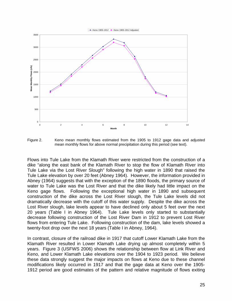
25
Figure 2. Keno mean monthly flows estimated from the 1905 to 1912 gage data and adjusted
mean monthly flows for above normal precipitation during this period (see text). Flows into Tule Lake from the Klamath River were restricted from the construction of a dike “along the east bank of the Klamath River to stop the flow of Klamath River into Tule Lake via the Lost River Slough” following the high water in 1890 that raised the Tule Lake elevation by over 20 feet (Abney 1964). However, the information provided in Abney (1964) suggests that with the exception of the 1890 floods, the primary source of water to Tule Lake was the Lost River and that the dike likely had little impact on the Keno gage flows. Following the exceptional high water in 1890 and subsequent construction of the dike across the Lost River slough, the Tule Lake levels did not dramatically decrease with the cutoff of this water supply. Despite the dike across the Lost River slough, lake levels appear to have declined only about 5 feet over the next 20 years (Table I in Abney 1964). Tule Lake levels only started to substantially decrease following construction of the Lost River Dam in 1912 to prevent Lost River flows from entering Tule Lake. Following construction of the dam, lake levels showed a twenty-foot drop over the next 18 years (Table I in Abney, 1964). In contrast, closure of the railroad dike in 1917 that cutoff Lower Klamath Lake from the Klamath River resulted in Lower Klamath Lake drying up almost completely within 5 years. Figure 3 (USFWS 2006) shows the relationship between flow at Link River and Keno, and Lower Klamath Lake elevations over the 1904 to 1923 period. We believe these data strongly suggest the major impacts on flows at Keno due to these channel modifications likely occurred in 1917 and that the gage data at Keno over the 1905-1912 period are good estimates of the pattern and relative magnitude of flows exiting
0
500
1000
1500
2000
2500
3000
3500
0 2 4 6 8 10 12 14
Month
Mea
n M
onth
ly F
low
s (c
fs)
Keno 1905-1912 Keno 1905-1912 Adjusted
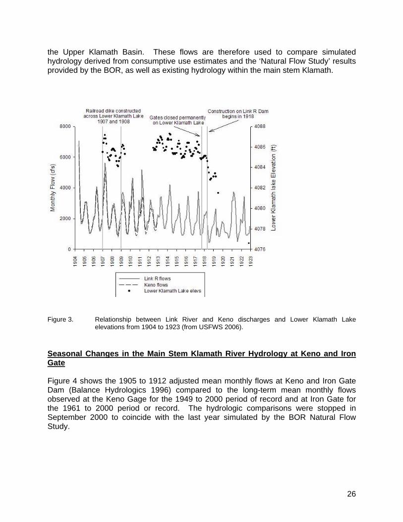
26
the Upper Klamath Basin. These flows are therefore used to compare simulated hydrology derived from consumptive use estimates and the ‘Natural Flow Study’ results provided by the BOR, as well as existing hydrology within the main stem Klamath.
Figure 3. Relationship between Link River and Keno discharges and Lower Klamath Lake
elevations from 1904 to 1923 (from USFWS 2006). Seasonal Changes in the Main Stem Klamath River Hydrology at Keno and Iron Gate Figure 4 shows the 1905 to 1912 adjusted mean monthly flows at Keno and Iron Gate Dam (Balance Hydrologics 1996) compared to the long-term mean monthly flows observed at the Keno Gage for the 1949 to 2000 period of record and at Iron Gate for the 1961 to 2000 period or record. The hydrologic comparisons were stopped in September 2000 to coincide with the last year simulated by the BOR Natural Flow Study.

27
Figure 4. Estimated historical mean monthly flows at Keno and Iron Gate compared to the mean
monthly flows at Keno (1949 to 2000) and Iron Gate (1961 to 2000). These data show that the peak flows in the hydrograph have shifted from April to March and that the mean minimum flows are lower. It is also apparent that the low-flow conditions during the summer period have also been extended compared to unimpaired historical conditions. Fall flows, however, are now higher. Quantitative assessments of changes in the hydrology suggest that the annual runoff volume from the upper basin has declined by about 370,000 acre-feet since construction of the Klamath Project and that the changes in the hydrograph are a direct consequence of water resource practices in the upper basin (Balance Hydrologics 1996, USGS 1995, NRC 2004). Klamath Project Operations and Flows downstream of Iron Gate Dam Iron Gate Dam was constructed as a re-regulating reservoir to reduce the impacts of peaking operations down stream of the Copco No. 2 powerhouse. The current license conditions from FERC require a minimum flow release of 1,300 cfs from September through April, 1,000 cfs in May and August, and 710 cfs in June and July; however, since 1996, the BOR Klamath Project Operations Plans have dictated instream flow releases based on water year type. License conditions also specify ramping rates of the lesser of 3 inches/hour or 250 cfs/hour. This is in contrast to the BOR operations plan down-ramping criteria that specifies:
(1) decreases in flows of 300 cfs or less per 24-hour period and no more than 125 cfs per 4-hour period when Iron Gate dam flows are above 1,750 cfs; and
0
500
1000
1500
2000
2500
3000
3500
4000
4500
Oct Nov Dec Jan Feb Mar Apr May Jun Jul Aug Sep
Month
Mea
n M
onth
ly F
low
s (c
fs)
Keno 1905-1912 Adjusted Keno 1949-2000 Observed Iron Gate 1905-1912 Adjusted Iron Gate 1961-2000 Observed

28
(2) (2) decreases in flow of 150 cfs or less per 4-hour period and no more than 50 cfs per 2-hour period when Iron Gate dam flows are 1,750 cfs or less.
PacifiCorp (2004) utilized RMA2 modeling simulations for the 2000 and 2001 period to evaluate the downstream impacts of their project facilities and the effects of the BOR Klamath Project, including a hypothetical no project condition. Figure 5 shows the hourly time series data for the no project versus project operations based on RMA2 simulations at Iron Gate and Seiad. What these simulation results illustrate is that project operations induce a much lower variation in the hourly flow regimes compared to the no project conditions and that these affects are propagated downstream over 40 miles below the confluence of both the Scott and Shasta River during low flow conditions. Although the facilities have ramping rate restrictions, stranding of young fish have been observed below Iron Gate Dam associated with changes in the base flow conditions (Tom Shaw, personal communication). It is important to note that although flow releases below Iron Gate constitute only a few percent of the total flow at the estuary during high flows, they can account for upwards of 45 to 75 percent of the total flow during late summer in critically dry periods. Under these conditions, exaggerated hourly flow fluctuations can be detrimental to young fish confined to the stream margins due to stranding and increase energetic costs associated with concurrent high water temperatures during these low flow periods.
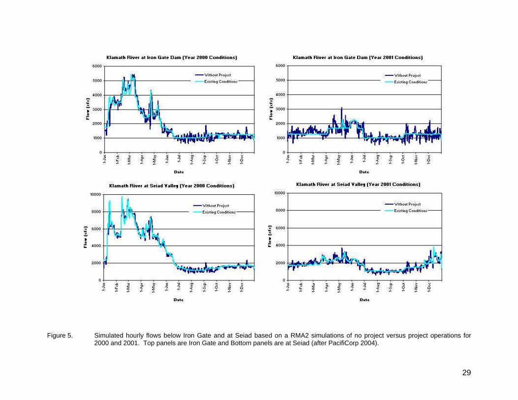
29
Figure 5. Simulated hourly flows below Iron Gate and at Seiad based on a RMA2 simulations of no project versus project operations for
2000 and 2001. Top panels are Iron Gate and Bottom panels are at Seiad (after PacifiCorp 2004).

30
PacifiCorp also analyzed the peak flow series for the period of record 1960-present downstream of Iron Gate dam (USGS Gauge No. 11516530) using the HEC-FFA model. Results of are shown in Table 1 and graphically in Figure 6. Table 1. Peak flow analyses below Iron Gate Dam 1960 to 2004 (after PacifiCorp 2004).
Estimated Peak Annual Return Period Exceedence Probability Flows at Iron Gate
Gauge (years) (%) (cfs)
100 1.0 38,200 50 2.0 31,100
20 5.0 23,000
10 10.0 17,600 5 20.0 12,700 2 50.0 6,830
1.25 80.0 3,600
Figure 6. Annual peak flows below Iron Gate Dam for the 1960 to 2004 period (after
PacifiCorp 2004). As noted in the section on geomorphic and riparian evaluations, these data suggest that larger flood events continue to occur within the river from the upper basin and given the cumulative affects of tributary inflows during many of these events, both channel and riparian maintenance flow processes are likely being maintained within the main stem Klamath River.

31
PacifiCorp (2004) also examined the annual low flow statistics below Iron Gate Dam for the 1960 to 2004 period and the results are provided in Table 2. Table 2. Annual low flow statistics below Iron Gate Dam for the 1960 to 2004 period (after
PacifiCorp 2004).
Annual Percent Chance of Occurrence
Days 50 20 10 5
1 689 593 562 543
3 694 597 565 547
5 700 601 569 549
7 703 603 570 550
30 757 637 579 532
Although extensive quantitative data based on daily flows for natural or unimpaired conditions are not available for the main stem Klamath River below Iron Gate Dam, ancillary data suggests that upstream depletions above Upper Klamath Lake in combination with depletions associated with the Klamath Project have altered the frequency and magnitude of low flows. The impact of the Klamath Project operations on monthly flows below Iron Gate Dam were estimated by PacifiCorp (2004) for the 1961 to 1997 period based on the BOR KPOPSIM model. These results are shown in Table 3. The simulations results suggest that during the spring, average depletions to the main stem Klamath River below Iron Gate Dam are greater than 50,000 ac-ft/mo (900+ cfs). Simulated Unimpaired and Natural Flows in the main stem Klamath River Given the lack of extensive pre-development hydrology for the main stem Klamath River, two different modeling approaches were undertaken by the BOR for use in the instream flow analyses. These modeling results were provided to USU for use in the Phase II assessments. The first approach relies upon a level-pool routing of Upper Klamath Lake using historical net inflows plus estimates of consumptive use depletions (i.e., accounts for upstream depletions) and no deliveries to the Klamath Project to estimate unimpaired flows. The second approach represents simulated natural flows at Keno developed by the BOR as part of their ‘Natural Flow Study’ (Perry et al., 2005).

32
Table 3. Monthly flow changes (in 1,000 ac-ft/mo) due to Klamath Irrigation Project operations predicted by KPOPSIM for the Klamath River below Iron Gate dam for the 1961-97 period (after PacifiCorp 2004). Note that 1,000 ac-ft/mo is approximately 17 cfs over the entire month.
Upper Klamath Lake Level Pool-Consumptive Use Based Estimated Unimpaired Hydrology The BOR provided estimated unimpaired monthly flows at Link River and Iron Gate (1961 to 2004 period) using a level pool routing in Upper Klamath Lake based on the observed net inflows to Upper Klamath Lake and adjusting the inflows to account for estimated consumptive uses. The monthly flows at Link River were then ‘routed’ downstream to Iron Gate Dam assuming no Klamath Project demands. These estimated flows ‘replace’ the original unimpaired flows utilized in the Draft Phase II report analyses. The flows originally used in the Draft Phase II analyses were developed as part of the Alternative Dispute Resolution process of the Upper Klamath Basin adjudication in Oregon and provided to USU. Subsequent to release of the Draft Phase II report, USU was informed that permission from ADR participants to use the original estimated unimpaired flows could not be obtained and therefore the BOR provided these independently derived flow estimates. Accretions between Upper Klamath Lake and Iron Gate Dam were based on those currently employed by the BOR in their operations models for the Klamath Project and therefore represent impaired accretions. USU used the level-pool routing consumptive use based estimated
Water Year Oct. Nov. Dec. Jan. Feb. Mar. Apr. May Jun. Jul. Aug. Sep. Total 1961 -17.3 -58.4 -34.9 -29.2 -113.1 -92 -37.2 -34.1 -14.2 30.4 -0.2 -6.9 -407.21962 -6.1 -4.9 -38.6 -13.9 -104.8 -113.4 -76.7 -73.8 3.7 22.7 2 3.7 -400.31963 -79.2 -12.2 -25.4 -10.9 -149.8 -27.3 -24.6 -27.6 -21 1.4 19.6 14.8 -342.31964 -11.7 -17 40.4 0.5 -42.8 -97.8 -72.9 -73.2 -69.1 0.6 5.6 14.1 -323.21965 16.3 -45.3 -260.8 51.5 70.6 90.6 -115.7 -106.4 -62.7 -28.7 -26.9 28.2 -389.21966 44.5 75.3 9 -14.1 -63.4 -134.2 -87.8 -61.9 -30.1 1.2 23.1 -15.2 -253.41967 0.4 -40.6 -30.1 -23.8 -20.6 -120.5 -82.3 -44.4 -68.7 10.9 22.8 13 -383.81968 -16.8 2.3 11.9 -47 -136.9 -45.7 -14.8 -30.5 3.3 7.5 -33.5 -23.6 -323.71969 -20.6 -61.8 -63.7 -94.8 -12.4 -89.2 -72.5 -60.7 -59.5 6 18.3 6.1 -504.81970 -18.3 39 -70.7 -151.8 14.6 -19 -68.4 -67.7 -32.6 1.4 40.5 -4.5 -337.61971 -37.1 -49.8 16.9 -76.7 -51.6 -80.3 2.2 -70.3 -66.3 -41.8 -0.3 -39.1 -494.21972 29.2 -3.8 24.5 -51.1 -69.9 -15.5 -62.8 -75.5 -64.6 -5.4 -15.9 -6.9 -317.61973 -23.7 2.4 -18.7 -21.4 -40.3 -54.4 -54.3 -51.1 9.9 12.4 -6.7 -42 -287.81974 -48.5 -126.1 -44.1 -44.2 -20.5 -41.4 -26.1 -81.6 -85.9 -42.3 -17.2 -18.4 -596.21975 -21.4 19.3 -2.4 -9.5 -42.7 -70.9 -47.5 -72 -97.9 -30.9 -12.8 -17.6 -406.21976 -0.4 10.9 17.7 -16.2 -36.1 -67.7 -76.9 -73.1 -38.9 -17.2 -65.5 -15.8 -379.21977 -11 37.3 -12.5 -21 -56.4 -103.8 -42.8 -57.2 -12.8 33.4 1.7 -27.6 -272.71978 -20.7 -68.8 -47.4 -35.1 -35.8 -57.1 -40.1 -42.7 -29.4 -10.1 12.2 -33.7 -408.61979 -14.8 -9.6 -28.4 -51 -68 -48.2 -60.5 -46.4 8.4 12.9 16.3 2.4 -286.91980 -39.8 -79.7 -86.9 -97.9 -50.3 -29.7 -60.7 -43.8 -32.3 5.8 38.2 -4.5 -481.51981 -8.1 -43.4 -70.9 -64.6 -91.2 -39.4 -35.1 -31.4 5.3 19.1 36.3 0.3 -323.21982 -56 -125.1 -94.8 10 -113.9 36.8 -19.6 -82.4 -94.8 1.9 3.3 -20.9 -555.51983 -17.3 20.1 8.2 -38.2 -80.2 -26.1 -47.9 -56.5 -57.9 -52.2 -35.6 -15.5 -399.21984 26.8 26.3 -2.7 -32.9 -52.4 -69.8 -42.5 -56.3 -67.5 -33.9 -19.4 -39.4 -363.51985 13.1 27.4 31.8 -38.1 -77.5 -90.9 -61.8 -67.8 -32.1 -0.3 -9.2 -38.9 -344.41986 -32.8 -29.8 16.9 -84.3 -97.9 -2.5 -44.1 -70.3 -46.9 -4.1 9.5 -44.5 -430.71987 -22.8 -42.1 -19.3 -63.2 -42.7 -64.6 -59.1 -27.7 -28.9 -21.1 -0.8 -3.2 -395.51988 -11 -33 -95.9 -75.9 -59.7 -67.4 -57.7 -40.8 -39.5 30.9 21.4 2.3 -426.21989 -22.3 -93.5 -55.2 -50.2 -31.9 -105.3 -63 -61.5 -19.7 16 8.7 -26.3 -504.11990 -28.9 -34.4 -32.6 -32.4 -41.3 -90.4 -51.9 -42.5 -20.3 7 -4.6 -8.3 -380.51991 -11.5 -26.7 -1.9 -54.7 -77.6 -115.5 -73.7 -62.3 -17.8 0.6 4.4 -14.4 -450.91992 -22.7 -61.5 -64 -61.5 -65.3 -74.6 -47.5 -13.8 10.4 -11.1 6.1 -11.6 -417.11993 -19.8 -52.8 -67.2 -73.2 -79.8 -151.1 -43 -71.5 -10.7 2.9 16.6 16.3 -533.41994 -21.4 -9 -39.9 -54.7 -67.5 -80.2 -56.8 -38.3 8.5 23.1 11.8 13.2 -311.21995 -11.7 -57.6 -52.1 -130.6 -146.1 -72 -51 -19 -51.2 -3.7 40.1 20.5 -534.31996 -6.4 -24 -142.7 -50.7 -41.2 -28.8 -53.4 -45 -10.4 7.7 3.3 -1.7 -393.31997 -29.9 -76.2 -136.7 -16.9 -20.9 -49.5 -78.4 -48.1 -18.6 -9 -4 -34.6 -522.6
-15.8 -25.4 -37.5 -45.5 -57.8 -58.5 -53.8 -55.1 -35.9 -4.7 2.3 -10.7 -398.3Average (1963-88, 1990-97)

33
monthly flows at Keno and added our estimated unimpaired accretions (see Estimation of Unimpaired Accretions below) to obtain flows at Iron Gate Dam. General modeling methods and results of flow routing through Upper Klamath Lake can be found in PWA (2002) while Appendix A provides a description of the methodology used by the BOR to derive the consumptive use based flows at Iron Gate Dam provided to USU. The monthly flow estimates below Iron Gate Dam for the 1961 to 2000 period were then routed to the estuary by adding estimated unimpaired accretions from tributaries on a monthly basis. Primarily the 1961 to 2000 period of record was utilized for comparative modeling since one of the tools used in our instream flow analysis, the System Impact Assessment Model (SIAM) (see discussion below), relies on this period of record. BOR Natural Flow Study Hydrology The other estimate of unimpaired flows is the BOR study by Perry et al., (2005) that derives estimated mean monthly ‘natural flows’ for the 1949 to 2000 period. These flows and the technical report are currently under review by the National Academy of Science but are used here as provided. We routed the monthly flows to the estuary and added our estimated unimpaired accretions from tributaries as described below. The 1961 to 2000 period of record was utilized for comparative simulations in SIAM; however, the full-simulated period of record is also utilized for some comparisons. Estimation of Unimpaired Accretions Estimations of the unimpaired accretions for tributaries from Keno to the estuary were derived from several sources. Spring inflow at J.C. Boyle was set at a constant value of 225 cfs based on the hydrologic summaries submitted by PacifiCorp as part of their re-licensing documentation. Estimated unimpaired monthly flows for the Shasta River (near Yreka, California) and the Scott River (at Fort Jones) were provided by the BOR for the1949 to 2000 period of record. The estimated flows for the Scott River at Fort Jones were adjusted to the confluence with the main stem Klamath River by adjusting the flows using the percentage of the drainage area between the two locations to account for additional tributary accretions. Unimpaired flows for the Salmon River were calculated using daily flows recorded at the USGS gage 11522500 (Salmon River at Somes Bar, California) for the period of record given the relative lack of impacts within the basin (USGS 1995, Balance Hydrologics 1996, NRC 2004). Estimated unimpaired flows for the Trinity River at Weitchpec were derived from a simple mass balance of the unimpaired daily flows at Hoopa plus the difference between the Hoopa flows and Lewiston Dam releases assuming a two day lag time (Scott McBain, personal communication). Summary tables and monthly time series plots for these main tributaries are provided in Appendix B. This appendix also provides the summary tables for estimated natural and unimpaired flows at Keno and Iron Gate Dam, which are graphically compared to existing flow conditions in the ‘Comparison of Estimated Hydrology’ section below.
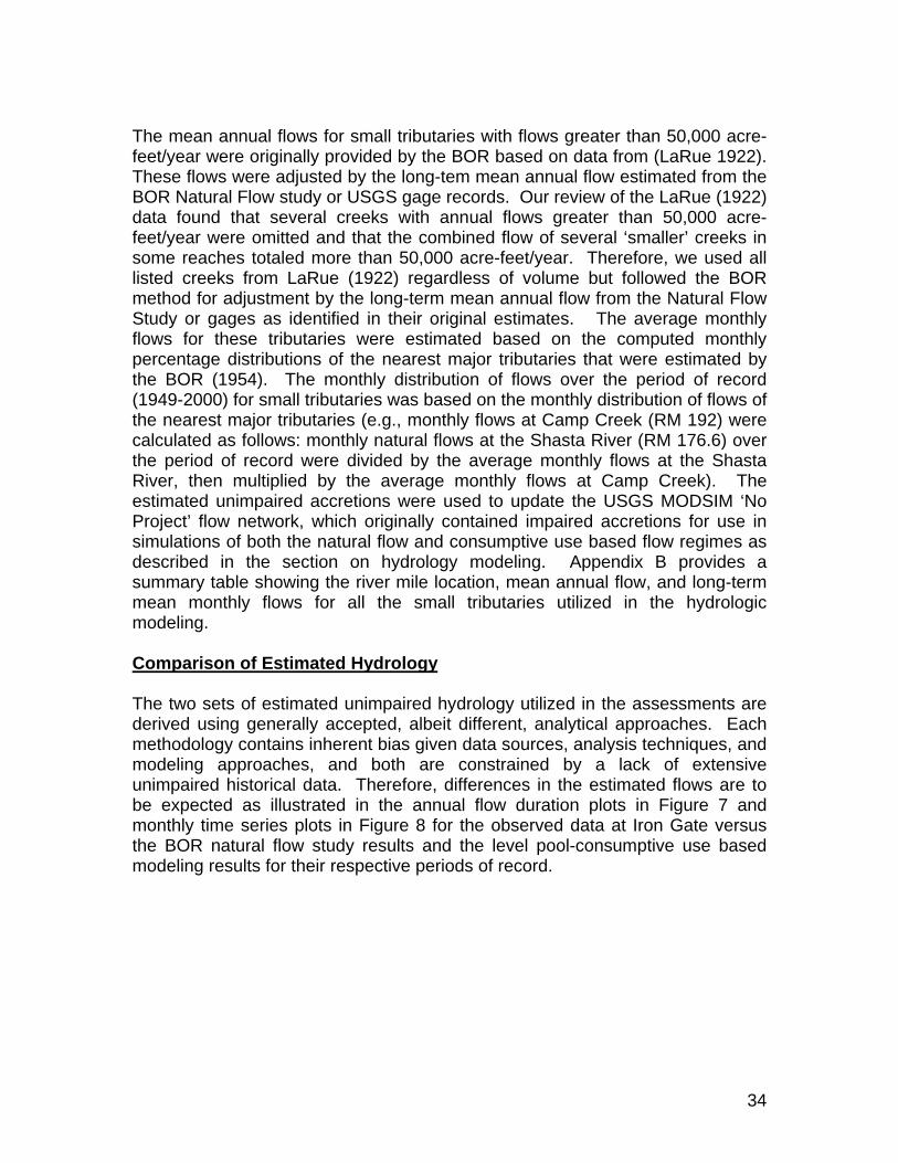
34
The mean annual flows for small tributaries with flows greater than 50,000 acre-feet/year were originally provided by the BOR based on data from (LaRue 1922). These flows were adjusted by the long-tem mean annual flow estimated from the BOR Natural Flow study or USGS gage records. Our review of the LaRue (1922) data found that several creeks with annual flows greater than 50,000 acre-feet/year were omitted and that the combined flow of several ‘smaller’ creeks in some reaches totaled more than 50,000 acre-feet/year. Therefore, we used all listed creeks from LaRue (1922) regardless of volume but followed the BOR method for adjustment by the long-term mean annual flow from the Natural Flow Study or gages as identified in their original estimates. The average monthly flows for these tributaries were estimated based on the computed monthly percentage distributions of the nearest major tributaries that were estimated by the BOR (1954). The monthly distribution of flows over the period of record (1949-2000) for small tributaries was based on the monthly distribution of flows of the nearest major tributaries (e.g., monthly flows at Camp Creek (RM 192) were calculated as follows: monthly natural flows at the Shasta River (RM 176.6) over the period of record were divided by the average monthly flows at the Shasta River, then multiplied by the average monthly flows at Camp Creek). The estimated unimpaired accretions were used to update the USGS MODSIM ‘No Project’ flow network, which originally contained impaired accretions for use in simulations of both the natural flow and consumptive use based flow regimes as described in the section on hydrology modeling. Appendix B provides a summary table showing the river mile location, mean annual flow, and long-term mean monthly flows for all the small tributaries utilized in the hydrologic modeling. Comparison of Estimated Hydrology The two sets of estimated unimpaired hydrology utilized in the assessments are derived using generally accepted, albeit different, analytical approaches. Each methodology contains inherent bias given data sources, analysis techniques, and modeling approaches, and both are constrained by a lack of extensive unimpaired historical data. Therefore, differences in the estimated flows are to be expected as illustrated in the annual flow duration plots in Figure 7 and monthly time series plots in Figure 8 for the observed data at Iron Gate versus the BOR natural flow study results and the level pool-consumptive use based modeling results for their respective periods of record.
35
Figure 7. Annual flow duration plots at Iron Gate for the observed and estimated flows based on the BOR natural flow study and level pool-consumptive use based methodologies.
Figure 8. Monthly time series plots at Iron Gate for the observed and estimated flows
based on the BOR natural flow study and level pool-consumptive use based methodologies.
0
2000
4000
6000
8000
10000
12000
0.0 10.0 20.0 30.0 40.0 50.0 60.0 70.0 80.0 90.0 100.0
Exceedence Probability, %
Flow
rate
, cfs
Consumptive Use UnimpairedBOR Nat. FlowImpaired
Klamath at Iron Gate (Gage 11516530)
Time Series - Klamath at Iron Gate (Gage 11516530)
0
1000
2000
3000
4000
5000
6000
7000
8000
Oct-60 Mar-66 Sep-71 Mar-77 Aug-82 Feb-88 Aug-93 Jan-99
Time
Flow
rate
, cfs
Consumptive Use UnimpairedBOR Nat. Flow

36
These results clearly show that the level pool-consumptive use based approach consistently generates higher estimated flows compared to the natural flow study. The flow exceedence plot (Figure 7) shows that the estimated natural flow or unimpaired flows are typically much higher than the impaired flows over most exceedence ranges. However, at low exceedence values (e.g., < 10%) the existing impaired flows are higher than the either the natural flows or unimpaired flows. We attribute this to the monthly time step used in the simulated unimpaired flows that do not reflect large daily flows recorded in the USGS gage data. The long-term mean monthly flows based on the natural flow study and level-pool routing hydrology are compared to the 1905-1912 adjusted flows at Iron Gate Dam in Figure 9.
Figure 9. Estimated mean monthly flows at Iron Gate Dam (1905 to 1912 adjusted from
Keno); the 1961-2000 period based on the BOR level-pool routing “consumptive use” based unimpaired and natural flow study results; and Iron Gate observed flows for the 1961-2000 period.
These data show that the consumptive use and natural flow study based results generally follow the seasonal pattern of the hydrograph when compared to the Iron Gate flows derived from the adjusted Keno gage readings over the 1905-1912 period. It appears that the natural flow study results may be under
0
500
1000
1500
2000
2500
3000
3500
4000
4500
Oct Nov Dec Jan Feb Mar Apr May Jun Jul Aug Sep
Month
Mea
n M
onth
ly F
low
s (c
fs)
Iron Gate 1905-1912 Adjusted Unimpaired Consumptive Use Natural Flow Study Iron Gate Impaired
37
predicting the flows during the February through about July period and over estimates the flows during November. However, the long-term averages during the August through October period are essentially the same as the adjusted historical Iron Gate flows. The consumptive use based estimates on the other hand appear to systematically overestimate the monthly flows except for the April through June period where they compare favorably with the adjusted historical Iron Gate flows. The results also show the impaired flows below Iron Gate Dam are much lower in the April through August period reflecting the Klamath Project operations. There are also somewhat higher flows with the impaired hydrology during the December and January period. Appendix C provides annual flow durations, monthly flow durations, and monthly time series result comparisons for the impaired (i.e., observed), natural flow study and level pool-consumptive use based modeling results for Keno, Iron Gate, Seiad, Orleans, and Klamath gages. Both the natural flow study and level-pool-consumptive use based modeling results at these gage locations contain the estimated unimpaired accretions developed by USU. The results show that as tributary accretions accumulate (e.g., the Seiad gage) the influence of these differences between modeling approaches become substantially less given the large volume of water in the main stem Klamath River below the Shasta and Scott Rivers. The monthly flow duration comparisons at Keno and Iron Gate also demonstrate the seasonal variability of these differences.
Water Quality and Temperature Evaluations The Klamath and Shasta Rivers are currently on the California 303(d) List of Impaired Water Bodies (California Environmental Protection Agency, accessed April 2004). The Klamath River was listed due to high water temperatures, low dissolved oxygen, and excess nutrients. The Shasta River was listed due to high water temperatures and low dissolved oxygen. These impaired conditions have been implicated as contributing factors associated with fish die-offs in the main stem Klamath River (NRC 2004, CDFG 2004, USFWS 2004). Based on an analysis of meteorological and water temperature data within the basin, Bartholow (2005) suggests that large-scale decadal climatic patterns may be inducing a warming trend of 0.58 C/decade in water temperatures, and if true, would pose an increased risk to all aquatic species in the river basin already exposed seasonally to acute/chronic ranges of temperature and associated disease factors. We consider temperature a critical factor in setting flow recommendations during all months of the year given the developmental, behavioral, and disease risk factors of anadromous species, thermal requirements of aquatic macroinvertebrates, and known thermal regimes within the main stem Klamath River. Temperature regimes control fish and other aquatic poikilotherms (e.g., macroinvertebrates) at the individual, population, and community levels (e.g., Beacham and Murray 1990, Huff et al., 2005, Ward and Stanford 1982). (NRC

38
2004) highlighted the thermal regime in the main stem Klamath in terms of its impact on coho, Chinook, and steelhead bioenergetics, importance of thermal refugia, and flow as key elements to consider in any flow recommendation. We defer our use and discussion of the ecological implications of water quality and temperature to the Evaluation and Justification of Proposed Flow Recommendations section of this report. Water Quality/Temperature Modeling An extensive body of empirical data and modeling results can be found in work supported by the Klamath Task Force (e.g., SIAM), Deas and Orlob (1999), PacifiCorp (2006) filings, CDFG (2004), USFWS (2003a, b), Flint and Flint (2006), migration studies (Strange 2006), and the thermal refugia work of Belchik (1997,2003). Additional empirical data (USFWS, unpublished field data) not found in the work cited above have also been incorporated into the report. Two different hydrologic/water quality “models” were used in the assessments. The first was the Systems Impact Assessment Model (SIAM) that incorporates both a water quantity component (MODSIM) and a water quality and temperature component (HEC-5Q). SIAM was utilized in the simulation of system behavior under several flow scenarios as described below. The second modeling approach relied upon simulation results from PacifiCorp (2006) developed as part of their Klamath Project re-licensing process and simulation modeling provided by the North Coast Regional Water Quality Control Board (NCRWQB 2006). These efforts relied upon RMA-2 (hydrodynamics) and RMA-11 (water quality/temperature) as part of the Klamath TMDL studies. These simulations were utilized for examination of differences in flows under their assumed ‘natural flow conditions’ for calendar year 2000 and existing conditions for the 2000 and 2002 calendar years. Risley and Rounds (2006) provides a broad based comparison between SIAM and RMA modeling systems applied in the Klamath and recommend that RMA be used for regulatory purposes. Presentation of water quality and modeling results in light of their ecological implications are deferred to the section on Instream Flow Recommendations. SIAM-MODSIM/HEC-5Q The Systems Impact Assessment Model (SIAM) (Bartholow et al., 2003) is a modeling interface used to simulate flow, water quality, and salmon production in the Klamath River under different flow alternatives. Three stand-alone models have been integrated into SIAM to achieve this purpose. The models are: MODSIM (flows), HEC-5Q (water quality), and SALMOD (fisheries). We primarily utilized the MODSIM and HEC-5Q components of SIAM to facilitate the modeling of hydrology and water quality below Iron Gate Dam for use in the physical habitat based assessments and instream flow recommendations.

39
MODSIM relies on a prioritization scheme for water allocations within a water resource network (Labadie 1988). MODSIM utilizes measured gage data and reservoir operation rules (i.e., storage, releases, and demands) on the main stem Klamath River under existing or for a ‘without project’ condition. The without project conditions approximates the routing of water from Upper Klamath Lake downstream to the estuary as if the Klamath Project did not exist and the PacifiCorp facilities were removed. MODSIM includes major tributaries (Shasta, Scott, Salmon, and Trinity Rivers) but they are not modeled except as inflow points using USGS gage records at or near their confluence with the Klamath River. Computational networks are composed of predefined river segment and node definitions that correspond to input or output locations for flows and water quality. These computational networks govern how the mass balance calculations are implemented for a specific ‘structure’ of the river system. Scott and Flug (1998) and Flug and Scott (1998) provide more specifics of the flow network for the Klamath River, calibration and validation, as well as the use of this simulation model for analyses. SIAM incorporates the HEC-5Q model developed by the U.S. Army Corps of Engineers Hydrologic Engineering Center’s HEC-5Q model (USACE 1986) to estimate water temperatures. A complete description of the HEC-5Q model adapted for the Klamath River can be found in Hanna and Campbell (2000). SIAM provides two preset flow scenarios and associated computational networks that were adopted for our analyses. The first represents the Klamath River ‘without’ the Klamath Project or dams (No Project) and the second (With Project) incorporates the existing water resource infrastructure. Both computational networks extend to the estuary. The ‘No Project’ computational network provided with SIAM utilized impaired accretions (Marshall Flug, USGS personal communication) and therefore was modified to incorporate the USU derived unimpaired accretions. This modified No Project network was used for simulation of the level-pool consumptive use and natural flow scenarios. The With Project network was used for all simulations under existing conditions and used impaired accretions as estimated by USGS. RMA-2/11 RMA2 is a two dimensional depth averaged finite element hydrodynamic numerical model that has been adapted to the Klamath River (Deas and Orlob, 1999; PacificCorp 2006, NCWQB 2006). RMA-11 uses the geometry and output of RMA-2 and solves the advection-diffusion equation to determine the fate and transport of up to 16 water quality constituents. These coupled models estimate within day thermal and water quality conditions important to understanding potential limiting factors. Simulations for the 2000 to 2004 calendar years for existing conditions and a ‘without project’ alternative were provided1. Detailed
1 USU had requested results for a derivative of the ‘Without Project’ alternative based on smoothing input flows referenced in Dunsmoor and Huntington (2006) but were refused access by PaCifiCorp owning to the status of their proceedings before FERC (July, 2006).
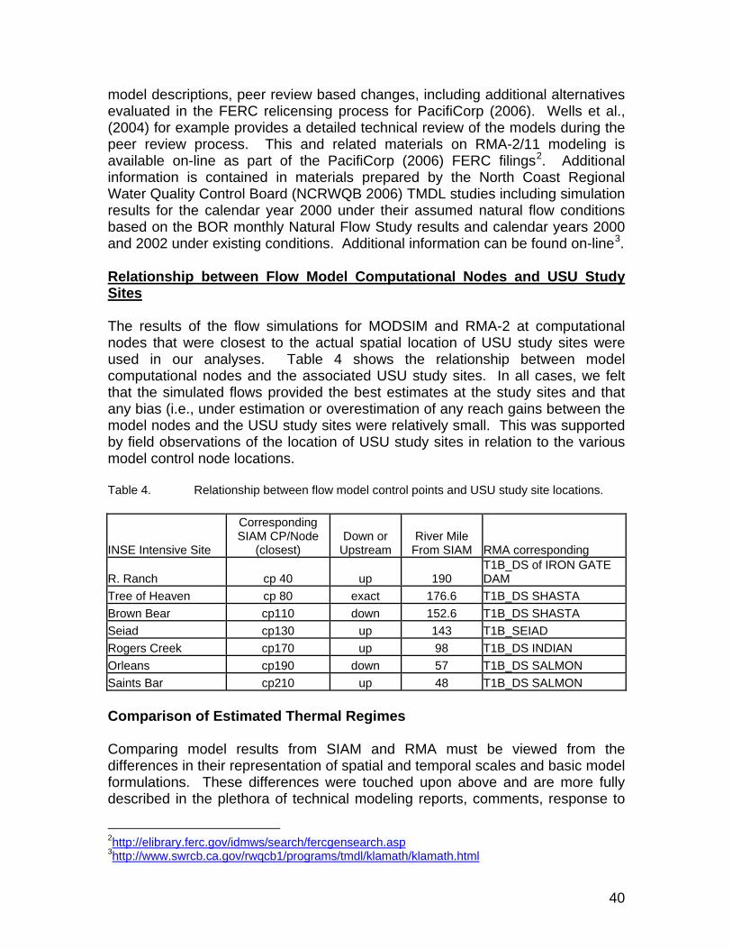
40
model descriptions, peer review based changes, including additional alternatives evaluated in the FERC relicensing process for PacifiCorp (2006). Wells et al., (2004) for example provides a detailed technical review of the models during the peer review process. This and related materials on RMA-2/11 modeling is available on-line as part of the PacifiCorp (2006) FERC filings2. Additional information is contained in materials prepared by the North Coast Regional Water Quality Control Board (NCRWQB 2006) TMDL studies including simulation results for the calendar year 2000 under their assumed natural flow conditions based on the BOR monthly Natural Flow Study results and calendar years 2000 and 2002 under existing conditions. Additional information can be found on-line3. Relationship between Flow Model Computational Nodes and USU Study Sites The results of the flow simulations for MODSIM and RMA-2 at computational nodes that were closest to the actual spatial location of USU study sites were used in our analyses. Table 4 shows the relationship between model computational nodes and the associated USU study sites. In all cases, we felt that the simulated flows provided the best estimates at the study sites and that any bias (i.e., under estimation or overestimation of any reach gains between the model nodes and the USU study sites were relatively small. This was supported by field observations of the location of USU study sites in relation to the various model control node locations. Table 4. Relationship between flow model control points and USU study site locations.
INSE Intensive Site
Corresponding SIAM CP/Node
(closest) Down or
Upstream River Mile
From SIAM RMA corresponding
R. Ranch cp 40 up 190 T1B_DS of IRON GATE DAM
Tree of Heaven cp 80 exact 176.6 T1B_DS SHASTA Brown Bear cp110 down 152.6 T1B_DS SHASTA Seiad cp130 up 143 T1B_SEIAD Rogers Creek cp170 up 98 T1B_DS INDIAN Orleans cp190 down 57 T1B_DS SALMON Saints Bar cp210 up 48 T1B_DS SALMON Comparison of Estimated Thermal Regimes Comparing model results from SIAM and RMA must be viewed from the differences in their representation of spatial and temporal scales and basic model formulations. These differences were touched upon above and are more fully described in the plethora of technical modeling reports, comments, response to
2http://elibrary.ferc.gov/idmws/search/fercgensearch.asp 3http://www.swrcb.ca.gov/rwqcb1/programs/tmdl/klamath/klamath.html

41
comments, and filings based on application the RMA system in the Klamath River FERC re-licensing process. Application of SIAM to the main stem Klamath below Iron Gate Dam by USGS has been noted throughout this report. The comparison of the estimated thermal regimes provides information about the various model behaviors and how they depart from reality, each other, flow or temperature bias (if any), and inherent uncertainty in making minimum, mean, and maximum temperature predictions at what locations in the river. The review by Risley and Rounds (2006) addresses some of these issues but more detailed discussion of boundary conditions and model parameters can be tracked through the PacifiCorp license filings and efforts of the Klamath TMDL process. We note the broader application of the RMA models within the institutional and regulatory setting (i.e., PacifiCorp and Klamath TMDL) as recommended by Risley and Rounds (2006) and therefore defer to the RMA simulations for much of our comparisons. SIAM is used to assess system trends over longer simulated periods not currently supported by the RMA models. Figures 10 compares the estimated flow and mean daily temperatures below Iron Gate for the 2000 and 2002 calendar years based on SIAM versus RMA approaches under existing conditions. Note in the SIAM based results the influence of the monthly time steps for the flow and daily time steps for the temperature, while the RMA models rely on daily hydrology and hourly time steps in computing temperatures. This is manifested most noticeably in the stair step nature of the simulated flow hydrographs. SIAM has some capacity to vary the flow regime within a month based on user-supplied heuristics but was not utilized in this study as noted below. Thermal buffering as a function of flow magnitude is reflected in the temperature plots and a reduction in the temporal variability starting in late summer and early fall. The temperature comparisons show that there can be a several degree difference between the two models on any given day and that the overall reduction in river temperatures are associated with the somewhat higher flows through early summer in 2000 compared to 2002 in both models. To further illustrate the differences in model behaviors, we compared the predicted mean daily temperatures below Iron Gate Dam using SIAM for the consumptive use, natural flow, and USGS no project alternatives and the RMA based no project simulations for the calendar year 2000 (see Figure 11).

42
Figure 10. Comparison of the flow and daily mean thermal regimes predicted using SIAM
and RMA modeling systems for the calendar year 2000 and 20002.
Figure 11. Comparison of SIAM and RMA simulated mean daily river temperatures below
Iron Gate Dam for calendar year 2000.
No Project Comparison (2000): Temperature
0
5
10
15
20
25
30
12/6/99 1/25/00 3/15/00 5/4/00 6/23/00 8/12/00 10/1/00 11/20/00 1/9/01 2/28/01
Date
Tem
pera
ture
, C
Consumptive Use Unimpaired BOR Nat. Flow USGS No Project RMA-11
43
It is apparent that the temperature simulations are somewhat sensitive to the input hydrology (i.e., compare the seasonal differences in temperature for the consumptive use and USGS no project based simulations). The RMA based results tend to show a much greater short term variance in sequential daily temperatures and exhibit a greater range in variability within a given time interval. A seasonal ‘flow induced bias’ between the different model simulations is also clear centered on a cross over point in approximately June in this example. We speculate that the seasonal pattern reflected by the ‘average daily temperatures’ of all the simulations likely reflects the underlying temporal characteristics of the thermal regime under natural conditions and that the range in the simulations are reflective of the temporal variability induced by stochastic meteorological conditions. We attempt to address model uncertainties, natural variability, and other aspects of the thermal regime in the section on Instream Flow Recommendations. In general, we rely on the RMA simulations where they are available and utilize SIAM only to examine at a courser level flow and temperature implications on flow regimes within the main stem Klamath given its longer simulation period capabilities. Assessment of Water Quality and Thermal Alterations The thermal regime below Iron Gate Dam is dominated by the shift in the seasonal hydrograph and flow magnitudes, the thermal buffering from main stem Klamath River dams, water resource project operations above Iron Gate Dam, and flow/temperature impacts associated with tributary systems. It is documented that existing project operations result in slightly cooler flows longer in the spring and more elevated temperatures are maintained in late fall due to the thermal mass of the reservoirs (NRC 2004, PacifiCorp 2006, Dunsmoor and Huntington 2006). The thermal buffering also manifests itself by a noticeable reduction in the daily minimum and maximum water temperature when compared to simulated conditions under a ‘no project’ alternative as illustrated in Figure 12 (e.g., see Dunsmoor and Huntington 2006).

44
Figure 12. Comparison of hourly temperature simulations below Iron Gate Dam under
Existing Conditions (EC) and the PacifiCorp (2006) Without Project (WOP). Inherently, the hydrologic shifts in timing and magnitude of flows propagate into changes in the thermal regime of the river below Iron Gate Dam. Analyses suggests that releases from the upstream system of reservoirs have likely increased October river temperatures and reduced July and August temperatures by a few degrees. Bartholow et al., (2005) used computer simulations to evaluate expected changes in Klamath River water temperatures and potential affects on Chinook life stages in the main stem Klamath River below Iron Gate ‘without dams’. Utilizing a flow release of ~ 38 cms that corresponds to a typical October flow and ~ 30+ percent of the flow at estuary, they suggest that the primary thermal affect of dam removal would be to shift the existing seasonal thermal regime approximately ~ 1-2 weeks earlier in the year with cooler overall water temperatures in the lower main stem. Conversely they speculate that the main stem would likely experience a wider range in daily water temperatures and an estimated increase in the average maximum daily temperature ~ 1.3°C in the mid-Klamath (i.e., Iron Gate to Seiad). They also note a loss of thermal damping associated with reservoir releases. Bartholow et al., (2005) caution that their results are only reliable in the Iron Gate Dam to Seiad reach of the river (i.e., the first ~ 110 river kilometers below the dam). PacifiCorp (2006) using hourly simulations for the 2000 to 2004 period under existing conditions and their ‘without project’ alternative generally concur with the general findings of changes in the thermal regime by Bartholow et al., (2005) within this same river reach.
Hourly Simulated Temperatures below Iron Gate Dam
0.00
5.00
10.00
15.00
20.00
25.00
30.00
1/1/20
00
1/15/2
000
1/29/2
000
2/12/2
000
2/26/2
000
3/11/2
000
3/25/2
000
4/8/20
00
4/22/2
000
5/6/20
00
5/20/2
000
6/3/20
00
6/17/2
000
7/1/20
00
7/15/2
000
7/29/2
000
8/12/2
000
8/26/2
000
9/9/20
00
9/23/2
000
10/7/
2000
10/21
/2000
11/4/
2000
11/18
/2000
12/2/
2000
12/16
/2000
12/30
/2000
Tem
pera
ture
(C)
WOP EC
45
At times, under combined basin wide low flow and warm climatic conditions, the flow induced thermal regime in the main stem Klamath River below Iron Gate Dame can be propagated over 238 km downstream (NRC 2004, Dunsmoor and Huntington 2006, Bartholow et al., 2005). Empirical data show that flow releases at Iron Gate Dam can make up more than the 30 percent of the flow at the estuary 238 km downstream (see example illustrated in Bartholow et al., (2005)). Changes in both flow and thermal regimes within tributary systems throughout the Lower Klamath Basin have also been impacted by anthropogenic factors and negatively affect the thermal regime within the tributaries as well as the main stem Klamath River (NRC 2004, Klamath TMDL, see additional references in the Estimated Unimpaired Hydrology Section). In many cases, habitat, flow, and thermal issues within tributaries are being addressed through active management practices (i.e., Trinity restoration program, CRIMPS, Klamath Task Force, Klamath River TMDL). These various modeling efforts however, provide an excellent insight into the expected thermal behavior of the system under more natural conditions4. We would postulate that in the late summer and early fall period, the main stem Klamath River in the region between Iron Gate Dam downstream to the vicinity of Seiad Valley would have had a more meteorological response system and in general, a greater between day and within day variation in the thermal regime compared to existing conditions as illustrated in Figure 12. We also maintain that the simulation results support the view that the length of periods and exposure times to deleterious thermal conditions were less under natural versus existing conditions. Dunsmoor and Huntington (2006) provided an excellent spatial and temporal comparison of existing conditions and without project thermal regimes below Iron Gate Dam based RMA simulations from 2000 to 2004 as shown in Figure 13 and 14.
4 We remind the reader that in the results for these particular models, the without project simulations utilized impaired inflows and accretions (see Dunsmoor and Huntington 2006) and therefore only indicative of expected results.
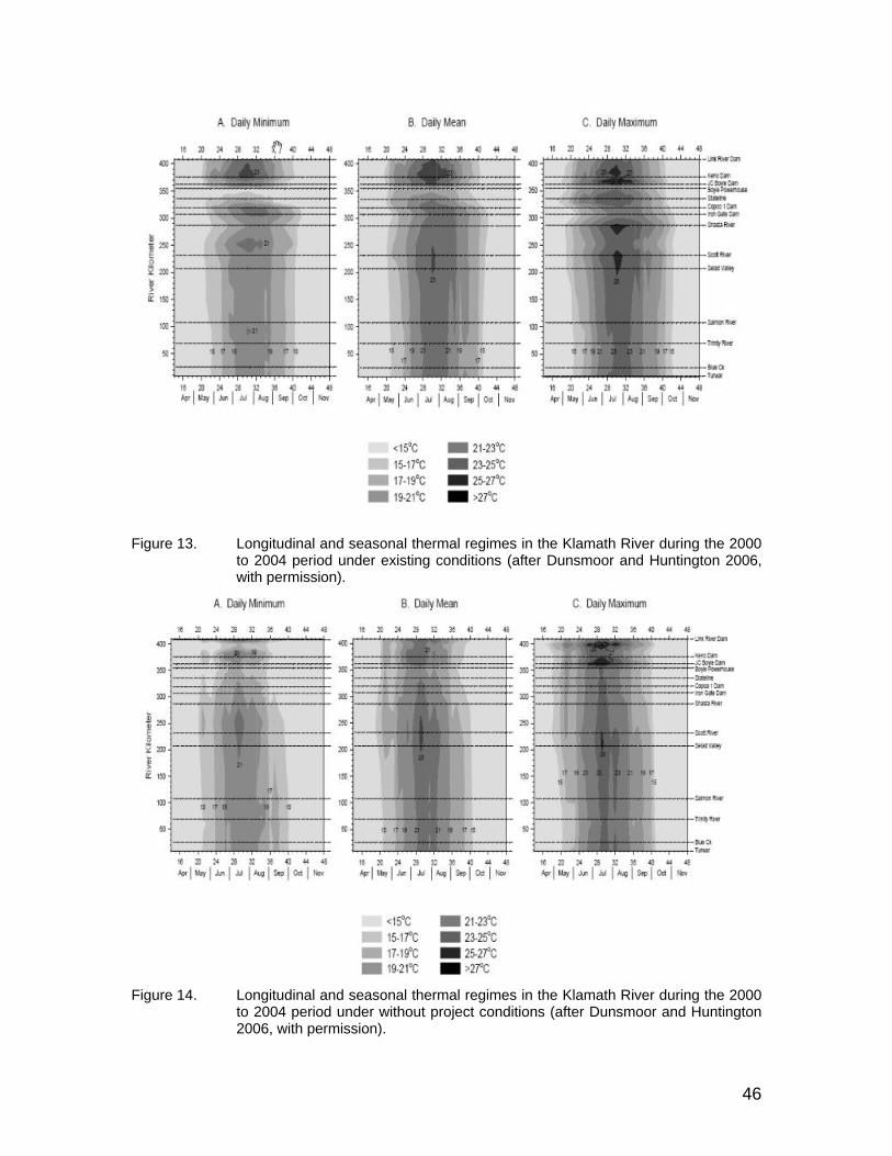
46
Figure 13. Longitudinal and seasonal thermal regimes in the Klamath River during the 2000
to 2004 period under existing conditions (after Dunsmoor and Huntington 2006, with permission).
Figure 14. Longitudinal and seasonal thermal regimes in the Klamath River during the 2000
to 2004 period under without project conditions (after Dunsmoor and Huntington 2006, with permission).

47
The results show that when the resulting temperature data are averaged over a week5 or 10 day period that the period of high summer temperatures is slightly narrower (less time with high temperatures) in the without project conditions than occurs for existing conditions. Also they show that the highest summer temperature occurs a bit sooner in the summer without project facilities than under existing conditions, but that later summer and fall temperatures remain cooler due to the thermal buffering of the reservoirs. The buffering affect is clearly manifested when the data of Dunsmoor and Huntington (2006) are plotted on a daily basis and reveals a much greater temperature variability in the section of the Klamath River where temperatures are currently tempered by the existing dams (i.e., below Iron Gate Reservoir). With “unimpaired” flows, there are increased peak temperature spikes as might be expected. These daily peak temperatures may actually increase the probability of exceeding acute temperature tolerances of fish. PacifiCorp (2006) and Dunsmoor and Huntington (2006) generally consider the downstream zone of influence due to operations at Iron Gate Dam to be ameliorated with increasing distance from the dam. They also note that from mid-July through August the existing project induces a delay in thermal response time seasonally, suppressed diel variability, which from mid-July through August, and may limit the periods of water temperatures less than 20°C. During the mid-August through September period, the delay in thermal cooling prorogates 112 km downstream to Seiad Valley. The without project temperatures were estimated to be frequently 3-5°C cooler than existing conditions below Iron Gate Dam at this time of year. Key findings from these studies on main stem Klamath River water temperatures are: 1) Higher flows in the spring from reservoir releases tend to be cooler than
would be expected under a natural flow regime due to the thermal mass in the reservoirs;
2) Thermal mass of the reservoirs is responsible for an increase in fall water temperature over what would be expected under a natural flow regime;
3) The reservoirs generally dampen the expected day-to-day and diurnal thermal cycle although releases below Iron Gate Dam imprints the flow and thermal signal downstream and reflects both operational changes in flow constrained by a limit on maximum turbine releases of 1735 cfs.
4) The operational zone of impact on the thermal regime is pragmatically confined from Iron Gate Dam downstream to the vicinity of Seiad Valley and dependant of flow release magnitudes at Iron Gate Dam.
The temporal and spatial implications of the thermal regime under recommended flows are considered later in the report. Based on the water quality simulations conducted to date in conjunction with the PacifiCorp re-licensing and the on-going TMDL for the Klamath Basin, we believe that dissolved oxygen and other 5 The Klamath TMDL process has proposed using the seven day average of the daily maximum temperature as part of their criteria, in part based on their review of the thermal literature.

48
water quality parameters are of secondary importance to our efforts compared to that of temperature.
Geomorphic and Riparian Evaluations An important aspect of providing flow recommendations that will protect the important physical, chemical, and biological processes of the river corridor relates to the dynamic processes associated with channel and riparian maintenance flows. This includes an assessment of existing channel conditions that may reflect anthropogenic disturbances and influence the assessment of instream flow needs based on the simulation of physical habitat and/or conditions necessary for salmon production. For example, it has been well documented that loss of flood flows within the Trinity River resulted in fossilization of point bars by mature riparian systems that ultimately resulted in a narrowing of the river channel and loss of alluvial functioning that directly and indirectly impacted young-of-the-year rearing habitat important to salmon production. Several studies of the Klamath River hydrology, geomorphology, riparian and channel form, and fish habitat have been conducted (Buer 1981, McBain and Trush 1995, Balance Hydrologics 1996, Ayres Associates 1999, PacifiCorp 2004). These studies generally document that historical anthropogenic activities associated with placer mining and sediment contributions from tributaries due to extensive logging impacted specific reaches within the main stem Klamath River. In addition, Iron Gate Dam (and upstream facilities) has resulted in trapping of sediments (Ayres 1999). There is some evidence that the bed material has become coarser but that fines are frequently flushed from pool and riffle habitats and that the bed remains mobile over flow ranges typically observed during normal and above normal water years. The primary area of impacted bed material below Iron Gate Dam is likely downstream to the confluence of Cottonwood Creek. Field observations on redd locations indicate suitable spawning gravels occur within a short distance downstream of the Dam although it is unclear if the quantity and/or quality of suitable spawning substrates have substantially changed from pre-dam (Iron Gate) conditions. A review of historical aerial photography over the 1955 to 2001 period (PacifiCorp 2006) suggests that the basic planform of the river at the reach scale has not changed over the past 50+ years. Localized changes were observed associated with tributary and in-channel mining activities (e.g., Humbug Creek, Trees of Heaven Campground, Seiad Valley). At these locations, the river channel was manipulated and the subsequent redistribution of large amounts of sediment in the river corridor altered the planform and bedform of the river. The downstream impacts from this redistribution of bed material are likely still occurring. Evidence suggests that most alluvial features and associated riparian vegetation communities remain dynamic.

49
Analyses conducted by Ayres (1999) and PacifiCorp (2004) suggest that riparian vegetation encroachment downstream of Iron Gate dam is not occurring due to the confined nature of the channel, frequent inundation, mobilization of the bed margins, and scour. This is further supported by flood frequency analyses, sediment transport analyses (PacifiCorp 2004), and observed flood events that show that flood magnitudes are sufficiently high and frequent to move most sediment fractions and cause substantial alterations in the riparian community structure and alluvial features throughout the main stem river corridor (see Table 1 and Figure 6 above).
Phase II Integrated Assessment Framework The primary objective for Phase II was to develop instream flow recommendations using best available science employing state-of-the-art field data collection and modeling techniques. This effort is focused on the use of physical habitat modeling as a central element although both temperature and salmon production estimates are also employed. The approach taken in Phase II focused on assessments of water quantity, temperature and water quality within the main stem Klamath River6 and relies on data, modeling results and supporting studies made available by collaborative efforts of state, federal and tribal resource agencies. The application and integration of the study components relied on a multidisciplinary assessment framework that parallels the Instream Flow Incremental Methodology (IFIM) developed by the U.S. Fish and Wildlife Service. This framework is illustrated in Figure 15. Figure 15 also illustrates the integrated nature of the physical, chemical, and biological processes and specific technical assessment components required to address instream flows in the main stem Klamath River. The initiation of the Strategic Instream Flow Assessment Plan component of this framework predates Phase I and Phase II. This component started with the identified need to assess the instream flow requirements in the main stem Klamath River as part of the objectives of the Klamath Restoration Act as well as on-going recovery actions by state, federal, tribal, local, and private groups. In addition, the USBR in collaboration with the USGS, BIA, USFWS, NMFS, Tribes, and the Technical Work Group from the Klamath River Basin Fisheries Task Force also facilitated the development of a long-term instream flow study plan for the Klamath River Basin to extend the work being conducted in Phase II.
6 USU initially proposed to incorporate tributary systems as part of the instream flow assessment process; however at the time, several members of the Klamath River Basin Fisheries Task Force opposed any instream flow assessment work in tributaries and therefore the study was confined to the main stem Klamath River below Iron Gate Dam.

50
Figure 15. Multidisciplinary assessment framework utilized for Phase II.
Phase II General Process The work conducted during Phase II followed a collaborative process and initially involved close coordination between USU and a technical review team. The team was composed of representatives of the U.S. Fish and Wildlife Service, Bureau of Reclamation, Bureau of Indian Affairs, U.S. Geological Survey, and the National Marine Fisheries Service. It also included participation by the Yurok, Hoopa Valley, and Karuk Tribes and the California Department of Fish and Game as the state level resource management agency. During the later part of the study process the technical team was expanded to include representatives of the Oregon Department of Fish and Wildlife, PacifiCorp, the Klamath Water Users Association and other interested parties/individuals. The expanded team reviewed all components of the study technical approaches in light of comments received from review of the draft report, and changes were made in analytical approaches where deemed appropriate.7,8 The technical team provided invaluable assistance throughout the study and provided data, analyses, supporting material for use in completion of the Phase II study. In addition, several agencies and private individuals provided written comments on the Preliminary Draft Report, which have been addressed where
7 The draft report was sent to three internationally recognized experts in instream flow assessments as well as a public review process that resulted in comments from 19 agencies, organizations, and individuals comprising 726 individual comments. 8 The only substantive remaining technical issue related to data collection, assessment methods, and analysis procedures not resolved during the complete review with the expanded team was how well existing study sites represented larger reaches of the river raised by the Klamath Water User Association technical consultant. Analyses begun by the consultant to document these concerns were never completed and interim data/results were not provided to the full technical team for review and evaluation. Therefore the existing data and methodologies for this component were unaltered.

51
appropriate. The Technical Team was utilized during the study for information and data exchange, technical discussions on methodologies, and review of study results. The team provided input and technical review for:
• Study design • Study reach selection • Study site selection • Field methods • Hydrology modeling • Hydraulic modeling calibration and simulations • Water quality modeling • Species and life stage periodicities • Species/life stage habitat suitability criteria development and validation • Habitat modeling development and validation • Integration of study results
In addition to technical review and input, most members of the Technical Team also provided technical assistance and collaborative efforts for field data collection and analyses. This included, for example, habitat mapping, collection of fish observation data, and analysis of habitat use data for development of habitat suitability criteria. Collaborative efforts are noted where appropriate throughout the remainder of the report. Based on the NRC (2005) review of the Texas Instream Flow Program9, the state adopted most of the committee’s recommendations when implementing their programmatic and technical instream flow programs. We closely follow the analytical and modeling techniques for field data collection, data reduction, hydraulic, aquatic habitat, water quality and temperature modeling adopted by the State of Texas based on the NRC (2005) review. Study Design The study design for the Phase II work was developed by USU after extensive discussions with state, federal, and tribal representatives during the Phase I process. This included input and discussions with the Technical Working Group of the Klamath Task Force. As noted previously, these discussions focused on specific technical approaches for:
a) The selection of study sites, b) Data collection strategies, c) Collaborative efforts with existing studies (e.g., USGS/USFWS
SIAM efforts), d) Analytical techniques, and e) Proposed modeling approaches for hydraulics, physical habitat, etc.
9 http://rio.twdb.state.tx.us/InstreamFlows/index.html

52
As noted above, the use of physical habitat modeling of salmonids parallels the conceptual application of the USFWS Physical Habitat Simulation System (PHABSIM) in terms of river reach stratification, habitat mapping, channel characterization, hydraulic model calibration and simulations, development of species habitat suitability criteria, habitat modeling, and integration of the habitat modeling with hydrology using habitat time series analyses. Each of these analytical components is described in the following sections. River Reach Stratification Input from the Technical Team was utilized to stratify the main stem Klamath River into ‘homogeneous’ study reaches. This stratification was primarily based on the junctions of major tributary systems within the main stem Klamath River. The purpose of this stratification was to delineate sections of river that function in a similar manner in terms of flow volumes and overall channel characteristics. The stratification also considered additional factors such as species and life stage distributions, access, locations of on-going fieldwork for other research (e.g., USGS/USFWS, Tribal fisheries programs), culturally sensitive areas for the tribes, existing modeling capabilities for water quantity and quality, and pragmatic factors dictated by time and budget constraints on field work for study site delineations. The Technical Team conducted a site reconnaissance of the main stem from Iron Gate Dam to the estuary as part of this stratification process. Based on the technical discussions and site reconnaissance, five river reaches were delineated:
1. Iron Gate Dam to the Shasta River 2. Shasta River to the Scott River 3. Scott River to the Salmon River 4. Salmon River to the Trinity River 5. Trinity River to the Estuary
These reach delineations are shown by different colors within the main stem Klamath River in Figure 16. Table 5 provides the starting, ending, and total length of river miles associated with each of these segments.

53
Table 5. Starting, ending, and total length of river miles for each river reach segment identified for Phase II studies.
Segments Iron Gate Dam
to Shasta River
Shasta River to Scott River
Scott River to Salmon River
Salmon River to Trinity River
Trinity River to Estuary
Starting Mile 0.00 13.45 46.94 125.23 148.10 Ending Mile 13.45 46.94 125.23 148.10 194.07 Segment Length (miles) 13.45 33.49 78.29 22.87 45.97 Overview of Study Site Selection The selection of study sites for Phase II were determined through a collaborative effort with the Technical Team and ongoing studies being conducted by the tribal, state, and federal resource agencies. Phase II study site locations were chosen to be broadly representative of channel characteristics within each delineated river reach and in some cases to overlap with existing USGS/USFWS SIAM study sites. These overlapping study sites were selected to permit comparison between USGS/USFWS study results with those generated in Phase II due to different field data collection and habitat modeling strategies between the two studies (1-dimensional cross-sections USGS/USFWS, 2-dimensional modeling USU). The process for selection of study sites involved the use of ground-based habitat mapping. This mapping effort characterized the available mesohabitats (i.e., fish habitat) within each river reach segment. Based on the mapping results, specific study site locations were selected based on the respective USGS/USFWS and Phase II study objectives.

54
Figure 16. River reach delineations, USGS/USFWS (1-D) and USU (intensive) study site
locations, river mile, and SIAM control point (CP) locations within the main stem Klamath River.
Habitat Mapping The USFWS, USGS, and Yurok Tribes undertook field-based mapping of mesohabitat types from Iron Gate Dam to the estuary. The mesohabitat classification scheme employed was developed by the USGS/USFWS SIAM study team in collaboration with other state, federal and tribal resource agencies and adopted for use in this study for consistency. The mesohabitat types were determined visually based primarily on gradient and secondarily on width, standing waves, presence of backwater and substrate (Table 6). Three levels of gradient were established: Low Slope (LS), Moderate Slope (MS), High Slope (HS) (same as Steep Slope (SS)), and Pools (P) as defined in Table 6. The gradients of 107 mesohabitats were measured in October and November 1996 with a Sokkia PowerSet 3000 as a way to verify visual determinations (Figure 17). A chi-square goodness of fit test was used to compare the frequency of mesohabitat types observed using visual estimation with the frequency of mesohabitat types expected based on defined gradients (Table 6).

55
There was no significant difference between observed and expected frequencies (p>.25) (USFWS 2004). Pools were defined as a reach controlled by a downstream hydraulic control. Runs were defined as having a low gradient and confined channel. Units that had characteristics of more than one mesohabitat type or were thought to fall in between two types were given a dominant and subdominant type. The dominant type was used for all data analysis. Starting at Iron Gate Dam, each mesohabitat unit encountered was enumerated, assigned to a specific mesohabitat classification, GPS coordinates delineated for the start of the feature, and maximum depth recorded with an acoustic bottom sounder. An Advantage Laser Atlanta laser range finder was used to determine lengths and widths of mesohabitat units. In addition main channel, side channels, and split channel classifications were made. According to the USGS/USFWS mapping protocol, a split channel was defined as a “permanent”, vegetated (trees) island that is not inundated even at a “high flow” (~ 10,000 cfs). A side channel has a temporary, un-vegetated or seasonally vegetated island (e.g., a gravel or sand bar) that is inundated by low or moderate flows (~ 3,000 – 6,000), typically annually. Whenever a split or side channel condition was encountered, mesohabitat mapping was conducted for the main channel and each side/split channel separately.
Figure 17. Mean gradient for mesohabitat types found between Iron Gate Dam and Seiad
Creek, October and November 1996. Error bars represent +/- 1 standard error (USFWS 2004).

56
Table 6. Criteria used to define mesohabitat types in the Klamath River from Iron Gate Dam to the confluence of Trinity River.
Mesohabitat Types
Criteria Pool Run Low Slope Moderate Slope
Steep Slope
Gradienta -- <0.3% <0.3% 0.3%-0.8% >0.8%
Channel Width
-- confined relatively unconfined
moderately confined
confined
Backwater yes no no no no
Substrate fines, sand, gravel --
gravel, small cobble
large cobble, small boulders
small and large boulders
Standing Waves none
<1/2' <1/2' 1/2'-1' >1'
aGradient = vertical drop / horizontal distance x 100 Table 7 provides a summary of the mesohabitat mapping results for each delineated river reach. The habitat mapping results were also utilized to extrapolate the modeled relationships between flow and available fish habitat within specific study sites to the reach level as described later in the report in the habitat modeling section. Note: The Trinity River to estuary reach has been omitted (see USU Two-dimensional Hydraulic Modeling section below).
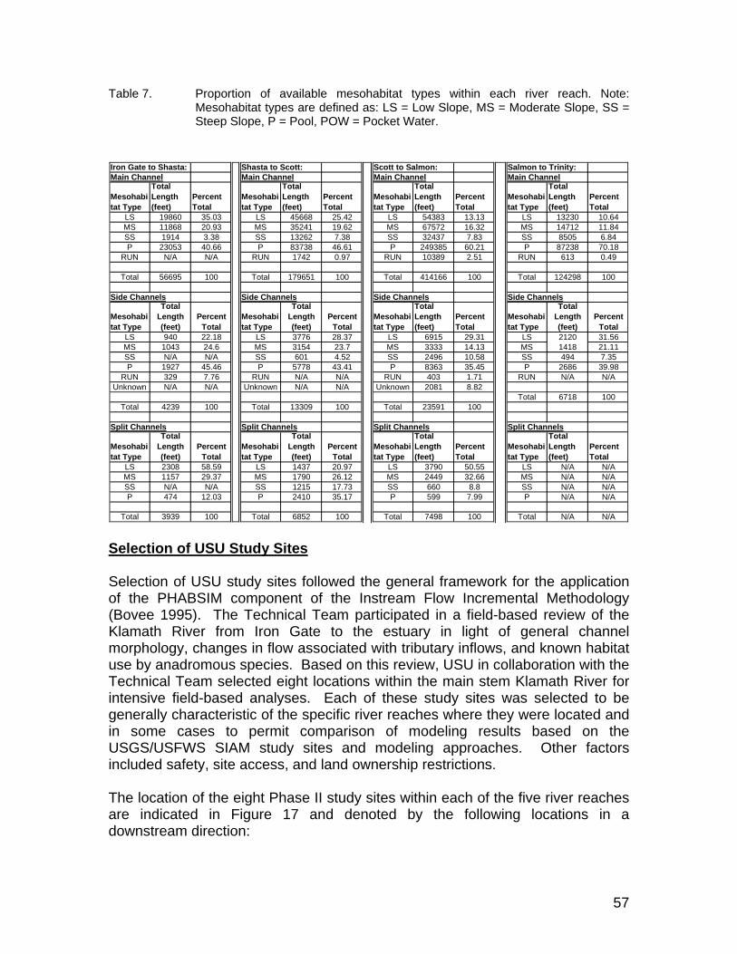
57
Table 7. Proportion of available mesohabitat types within each river reach. Note: Mesohabitat types are defined as: LS = Low Slope, MS = Moderate Slope, SS = Steep Slope, P = Pool, POW = Pocket Water.
Selection of USU Study Sites Selection of USU study sites followed the general framework for the application of the PHABSIM component of the Instream Flow Incremental Methodology (Bovee 1995). The Technical Team participated in a field-based review of the Klamath River from Iron Gate to the estuary in light of general channel morphology, changes in flow associated with tributary inflows, and known habitat use by anadromous species. Based on this review, USU in collaboration with the Technical Team selected eight locations within the main stem Klamath River for intensive field-based analyses. Each of these study sites was selected to be generally characteristic of the specific river reaches where they were located and in some cases to permit comparison of modeling results based on the USGS/USFWS SIAM study sites and modeling approaches. Other factors included safety, site access, and land ownership restrictions. The location of the eight Phase II study sites within each of the five river reaches are indicated in Figure 17 and denoted by the following locations in a downstream direction:
Iron Gate to Shasta: Shasta to Scott: Scott to Salmon: Salmon to Trinity:Main Channel Main Channel Main Channel Main Channel
Mesohabitat Type
Total Length (feet)
Percent Total
Mesohabitat Type
Total Length (feet)
Percent Total
Mesohabitat Type
Total Length (feet)
Percent Total
Mesohabitat Type
Total Length (feet)
Percent Total
LS 19860 35.03 LS 45668 25.42 LS 54383 13.13 LS 13230 10.64MS 11868 20.93 MS 35241 19.62 MS 67572 16.32 MS 14712 11.84SS 1914 3.38 SS 13262 7.38 SS 32437 7.83 SS 8505 6.84P 23053 40.66 P 83738 46.61 P 249385 60.21 P 87238 70.18
RUN N/A N/A RUN 1742 0.97 RUN 10389 2.51 RUN 613 0.49
Total 56695 100 Total 179651 100 Total 414166 100 Total 124298 100
Side Channels Side Channels Side Channels Side Channels
Mesohabitat Type
Total Length (feet)
Percent Total
Mesohabitat Type
Total Length (feet)
Percent Total
Mesohabitat Type
Total Length (feet)
Percent Total
Mesohabitat Type
Total Length (feet)
Percent Total
LS 940 22.18 LS 3776 28.37 LS 6915 29.31 LS 2120 31.56MS 1043 24.6 MS 3154 23.7 MS 3333 14.13 MS 1418 21.11SS N/A N/A SS 601 4.52 SS 2496 10.58 SS 494 7.35P 1927 45.46 P 5778 43.41 P 8363 35.45 P 2686 39.98
RUN 329 7.76 RUN N/A N/A RUN 403 1.71 RUN N/A N/AUnknown N/A N/A Unknown N/A N/A Unknown 2081 8.82
Total 6718 100Total 4239 100 Total 13309 100 Total 23591 100
Split Channels Split Channels Split Channels Split Channels
Mesohabitat Type
Total Length (feet)
Percent Total
Mesohabitat Type
Total Length (feet)
Percent Total
Mesohabitat Type
Total Length (feet)
Percent Total
Mesohabitat Type
Total Length (feet)
Percent Total
LS 2308 58.59 LS 1437 20.97 LS 3790 50.55 LS N/A N/AMS 1157 29.37 MS 1790 26.12 MS 2449 32.66 MS N/A N/ASS N/A N/A SS 1215 17.73 SS 660 8.8 SS N/A N/AP 474 12.03 P 2410 35.17 P 599 7.99 P N/A N/A
Total 3939 100 Total 6852 100 Total 7498 100 Total N/A N/A
58
1. RRanch 2. Trees of Heaven 3. Brown Bear 4. Seiad 5. Rogers Creek 6. Orleans 7. Saints Rest Bar 8. Young’s Bar10
Note in Figure 17 that the USGS/USFWS SIAM study sites are labeled to show where overlapping study sites exist between these two efforts. Channel Characterization The field methodologies used by USU for Phase II to characterize the channel at each study site delineated the channel characteristics (i.e., channel topography, substrate, and vegetation) in a spatially explicit manner over the entire study site. This approach to field data acquisition was based on data suitable for application of 2-dimensional hydraulic and habitat modeling. The use of this type of hydraulic modeling requires that 3-dimensional topography be collected for the each study site as illustrated in Figure 18. We assume that existing confined canyon areas and alluvial sections will remain in their approximate spatial locations and in roughly the same proportions as reflected in the habitat mapping data. We expect that dynamic transport of bed load and variable sized suspended load (physical and biological) is to be expected and likely alter smaller scale attributes within the major mesoscale features (i.e., low slope, moderate slope habitats). We believe this is an assumption that is supported by a number of analyses (e.g., Ayers 1999, PaciFiCorp 2006). Although these localized changes in channel topography (and vegetation responses to flow) were not modeled in this study, we maintain that the basic channel characteristics are provided by the study site results. More integrated modeling of the dynamic processes between flow, sediment movement, changes in channel topography and substrate characteristics that incorporate riparian vegetation succession modeling to project future conditions for anadromous rearing habitats is being undertaken as part of the Trinity Restoration Program and were beyond the scope of this study. USU Field Methodologies for Channel Characterization The 3-dimensional topography was generated by using low elevation high-resolution aerial softcopy photogrammetry and GPS linked hydroacoustic-based mapping of the channel topography. The aerial photogrammetry was utilized to acquire channel topographies that were above water, while the acoustic-based 10 This site was subsequently dropped from further analyses based on unsatisfactory data for the hydrodynamic modeling as discussed in the Hydraulic Modeling Section.
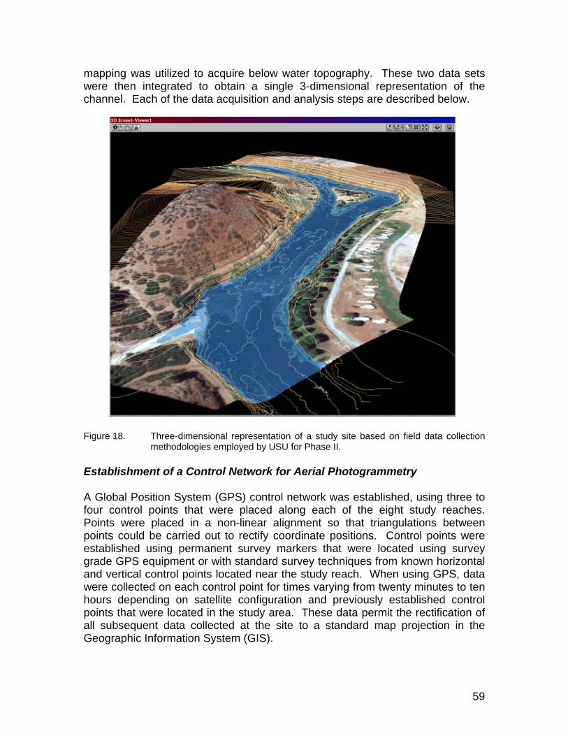
59
mapping was utilized to acquire below water topography. These two data sets were then integrated to obtain a single 3-dimensional representation of the channel. Each of the data acquisition and analysis steps are described below.
Figure 18. Three-dimensional representation of a study site based on field data collection
methodologies employed by USU for Phase II. Establishment of a Control Network for Aerial Photogrammetry A Global Position System (GPS) control network was established, using three to four control points that were placed along each of the eight study reaches. Points were placed in a non-linear alignment so that triangulations between points could be carried out to rectify coordinate positions. Control points were established using permanent survey markers that were located using survey grade GPS equipment or with standard survey techniques from known horizontal and vertical control points located near the study reach. When using GPS, data were collected on each control point for times varying from twenty minutes to ten hours depending on satellite configuration and previously established control points that were located in the study area. These data permit the rectification of all subsequent data collected at the site to a standard map projection in the Geographic Information System (GIS).
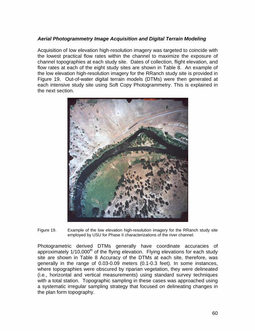
60
Aerial Photogrammetry Image Acquisition and Digital Terrain Modeling Acquisition of low elevation high-resolution imagery was targeted to coincide with the lowest practical flow rates within the channel to maximize the exposure of channel topographies at each study site. Dates of collection, flight elevation, and flow rates at each of the eight study sites are shown in Table 8. An example of the low elevation high-resolution imagery for the RRanch study site is provided in Figure 19. Out-of-water digital terrain models (DTMs) were then generated at each intensive study site using Soft Copy Photogrammetry. This is explained in the next section.
Figure 19. Example of the low elevation high-resolution imagery for the RRanch study site
employed by USU for Phase II characterizations of the river channel. Photogrametric derived DTMs generally have coordinate accuracies of approximately 1/10,000th of the flying elevation. Flying elevations for each study site are shown in Table 8 Accuracy of the DTMs at each site, therefore, was generally in the range of 0.03-0.09 meters (0.1-0.3 feet). In some instances, where topographies were obscured by riparian vegetation, they were delineated (i.e., horizontal and vertical measurements) using standard survey techniques with a total station. Topographic sampling in these cases was approached using a systematic irregular sampling strategy that focused on delineating changes in the plan form topography.

61
Table 8. Dates of image collection, flight elevations, and flow rates measured at the eight USU study sites. Note that the flight elevations are in meters.
Aerial Photogrammetry Data Reduction Aerial photography ground control targets were placed on the ground at each intensive study site and surveyed with GPS using the survey control network. All survey data were submitted to standard QA/QC checks at each site. This included for example, satellite configuration errors, checks on ellipsoid height errors, PDOP (point dilution of precision), L1/L2 fix statistics, etc. The aerial targets were used as horizontal and vertical control in the photogrammetry block adjustment process. Aerial photographs were scanned at 12 um using a high quality photogrammetric scanner. The interior orientation of each image was set in the photogrammetry software using the USGS camera calibration report parameters for the aerial camera. The ground control points in combination with between image tie-points were used within the photogrammetry software to perform a least-squares block bundle adjustment of all images. Statistics from this process were reviewed for accuracy with an allowable maximum Root Mean Square Error of 1.0 or less. Following this step, stereo pairs for use in digital terrain modeling were generated. The three-dimensional topography (DTM’s of above water topography) was then generated from the stereo pairs using standard softcopy
RRanch 8/24/1999 1-02 1059.809 1140 Youngs Bar 8/24/1999 9-05 481.776 30381-03 1064.617 9-07 456.7121-04 1065.222 9-08 464.5561-05 1058.915 9-09 467.831Average: 1062.141 9-10 470.365
9-11 471.526Seiad 8/24/1999 4-04 822.387 1470 Average: 468.794
4-05 826.8314-06 829.635 Trees of Heaven 8/24/1999 2-01 1014.172 12244-07 828.622 2-02 1018.8824-08 826.980 2-03 1025.2644-11 822.099 2-04 1032.1564-12 825.476 2-05 1041.4284-13 828.856 2-06 1048.0514-14 831.083 Average: 1029.9924-15 828.1804-16 821.511 Rogers Creek 8/24/1999 5-01 568.423 1832Average: 826.515 5-02 570.465
5-03 574.068Orleans 8/24/1999 6-03 521.449 2130 5-04 575.765
6-04 519.932 5-05 579.9706-05 515.774 5-06 585.3946-06 512.974 5-09 563.3586-07 510.109 5-10 571.0516-08 503.838 5-11 578.8136-09 507.045 Average: 574.1456-10 509.0996-11 511.487 Saints Rest Bar 8/24/1999 7-02 472.690 2130Average: 512.412 7-03 479.986
7-04 492.593Brown Bear 8/24/1999 3-06 915.235 1226 7-05 499.833
3-07 921.588 7-06 505.8183-08 927.421 Average: 490.1843-09 930.2483-10 932.148Average: 925.328
Flow Rate (cfs)Sites
Date of Image Collection
Image Frame
Flight Elevations Sites
Flow Rate (cfs)
Flight Elevations
Image Frame
Date of Image Collection
62
photogrammetry techniques. All topography work was reviewed by a second research technician as a QA/QC check. Following generation of the complete DTM’s, digital orthophotographs were produced for each study site. The orthophotographs were then used for the development of a GIS base map for each study site. This GIS (orthophotograph) base map was used primarily to overlay data from fisheries observations, substrate/cover mapping, hydrodynamic modeling (including computational meshes), topography contours, and fish habitat modeling results as described below. The orthophotographs for each of the eight study sites are provided in Figures 20 through 27. Hydro-acoustic Mapping of Underwater Topography and Data Reduction The hydroacoustic based mapping of the subsurface channel topography (i.e., under water topography) was undertaken with a boat mounted real-time kinematic differentially corrected survey grade GPS system integrated with a scientific grade single beam acoustic bottom profiling system. An acoustic doppler current profiling system (ADP) for measurement of the 3-dimensional velocity profile throughout the water column and depth was also integrated into the instrument package. The integrated boat mounted instrument package is shown in Figure 28. The hydroacoustic mapping was conducted at a discharge that was greater than the discharge at which the aerial photogrammetry was collected to ensure an overlap between the DTMs generated from these data sets and to minimize the potential for missing topographies where the acoustic mapping was limited by water depths at the stream margins. Figure 29 illustrates a typical GPS track of the USU integrated boat mounted hydro-acoustic mapping instrument package while collecting bottom topographies at a river site. This figure also illustrates out of water terrain points derived from soft copy photogrammetry. Table 9 lists the dates, flow rates, and number of sample points collected when acoustic mapping was conducted at each USU study site. Hydro-acoustic data reduction involved conversion of electronic data from field systems in the laboratory, data censoring, and QA/QC of the raw field data. Data censoring and QA/QC procedures were used to remove any data points where either bottom lock was lost on the hydro-acoustic profiling gear or GPS location data were degraded outside acceptable limits. In addition, the data were screened visually in the 3-dimensional photogrammetry software for outliers where shallow water interference caused errors in the hydro-acoustic data.

63
Figure 20. Orthophotograph of the USU RRanch study site.
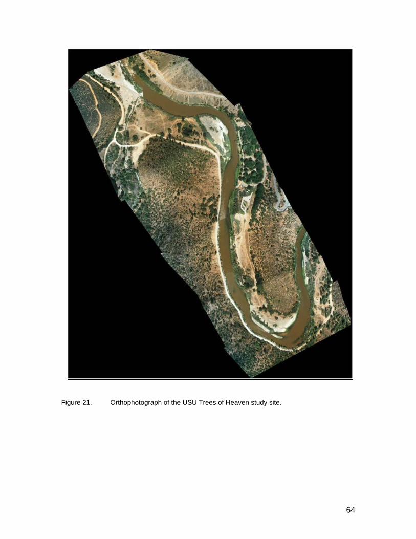
64
Figure 21. Orthophotograph of the USU Trees of Heaven study site.

65
Figure 22. Orthophotograph of the USU Brown Bear study site.

66
Figure 23. Orthophotograph of the USU Seiad study site.

67
Figure 24. Orthophotograph of the USU Rogers Creek study site.

68
Figure 25. Orthophotograph of the USU Orleans study site.
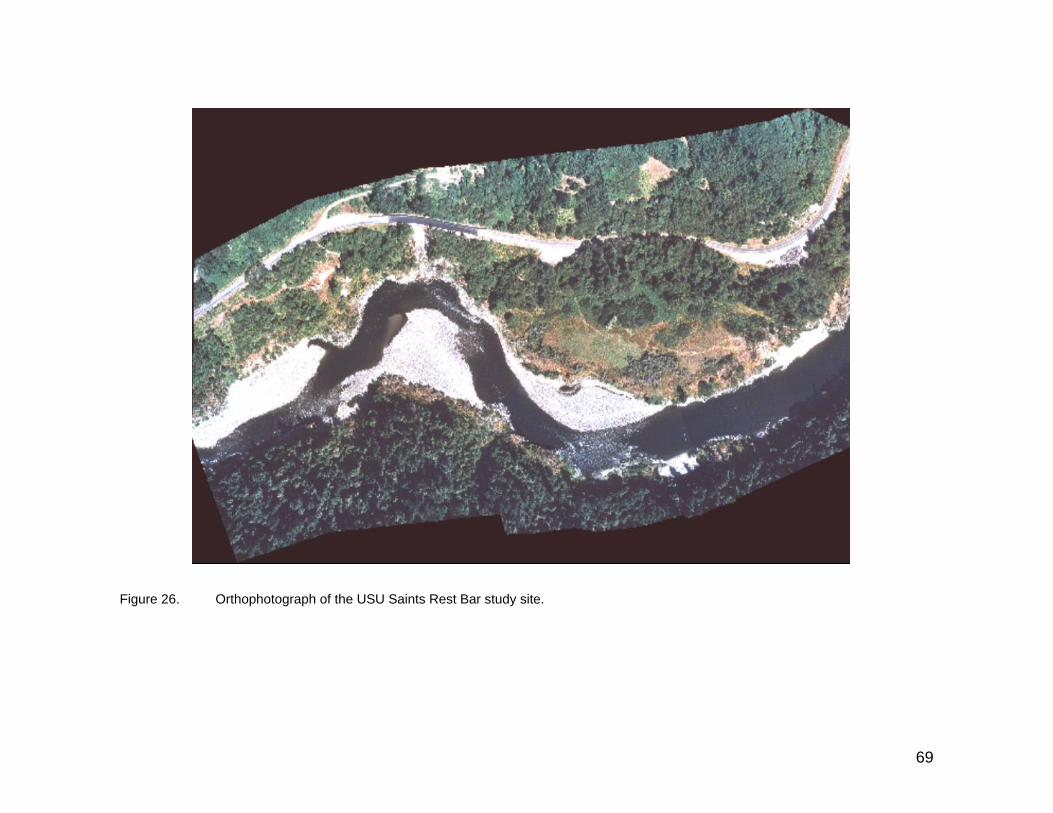
69
Figure 26. Orthophotograph of the USU Saints Rest Bar study site.

70
Figure 27. Orthophotograph of the USU Young’s Bar study site (Note: This site was dropped from further analyses based on poor
calibration of the hydrodynamic model as discussed in the Hydraulic Modeling Section).
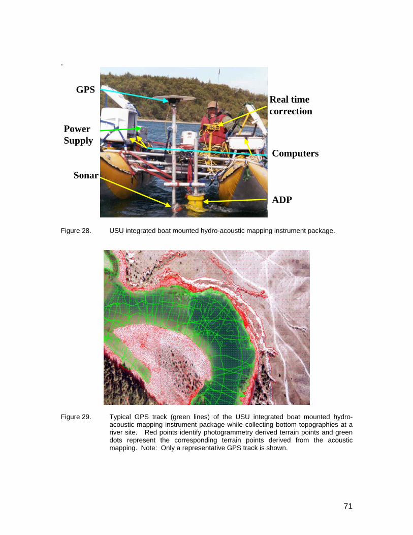
71
.
Figure 28. USU integrated boat mounted hydro-acoustic mapping instrument package.
Figure 29. Typical GPS track (green lines) of the USU integrated boat mounted hydro-
acoustic mapping instrument package while collecting bottom topographies at a river site. Red points identify photogrammetry derived terrain points and green dots represent the corresponding terrain points derived from the acoustic mapping. Note: Only a representative GPS track is shown.
GPS
Sonar
Computers
ADP
Real timecorrection
PowerSupply

72
Table 9. Dates, flow rates, and number of data points collected during acoustic mapping at each intensive study site.
Study Site Collection Dates Flow Rate(s) CFS Number of
Sonar Points RRanch 3/29-3/30/99 5550,5530 18540
Trees of Heaven 3/25-3/27/99 6496 36400 Brown Bear 3/23-3/24/99 7563 22021
Seiad 3/16-3/20; 3/22/99 10300,9490,9220,10900,12600,1160 47407 Rogers Creek 8/26-8/27/99 1832 6970*
Orleans 4/1-4/3/99 16700,16900 23439 Saints Rest Bar 4/6/1999 16600,16500 9893
Young’s Bar 4/7-4/8/99 22580,22500 14677 * Data collected using ADP. All other data collected using single beam sonar. Integration of Photogrammetry and Hydro-acoustic Data The integration of the DTM data derived from the softcopy photogrammetry and the DTM data derived from the hydro-acoustic data were integrated with conventional survey data to generate a single spatially explicit terrain model for each intensive study site. This terrain model was then used to develop 3-dimensional computational meshes for input into the 2-D hydrodynamics (i.e., hydraulic) model for each study site. The development of the computational meshes and hydrodynamic modeling is discussed below. Water Surface Elevation and Water Velocity Mapping The longitudinal profile of the water surface elevation within each study site was measured at a minimum of three calibration discharges. The survey data was tied directly to the upstream and downstream control cross sections at each intensive site. These water surface profiles were accompanied by an estimate of the discharge at the site. The discharge and water surface elevation data sets were used for 2-dimensional hydrodynamic model calibration as described below. Velocity measurements using a three-dimensional acoustic doppler current profiler (ADCP) were undertaken throughout the study sites at the discharge associated with the delineation of the channel topographies. Table 10 indicates the dates of hydraulic calibration data set collections and associated flow rates at each USU study site.
73
Table 10. Dates of collection and flow rates for each calibration data set at USU study sites (WSE = Water Surface Elevation at the downstream boundary of the site, cms = cubic meters per second).
Substrate and Vegetation Mapping Substrate and vegetation distributions were mapped at each study site by delineating field interpreted polygons on color aerial photograph prints and then digitizing these polygon data in the laboratory. Substrate and vegetation codes were standardized for the study and are provided in Table 11. Where substrate could not be delineated directly, snorkeling, and underwater video were utilized. This work was undertaken through a collaborative effort by the Yurok Tribal fisheries resource personnel assisting with the Phase II work. The digitized polygon data were then overlaid onto the orthophotographs in GIS in order to assign variable roughness values spatially within a study site at each computational mesh node location for use in the hydraulic modeling. As will be discussed below, the integration of the substrate and vegetation mapping with the hydraulic solutions at each computational mesh node were also used in the habitat modeling for fish. Figures 30 through 37 show the substrate and vegetation polygon distributions delineated for each intensive study site and overlaid on the study site orthophotographs.
Site Date High WSE (m) High Q (cms) Med WSE (m) Med Q (cms) Low WSE (m) Low Q (cms)Rranch 3/29/1999 624.99 157.164Rranch 6/3/1999 624.24 53.800Rranch 8/24/1999 623.99 32.280Trees of Heaven 3/27/1999 566.41 183.953Trees of Heaven 6/2/1999 565.29 57.599Trees of Heaven 8/24/1999 564.94 34.661Brown Bear 3/23/1999 471.23 214.168Brown Bear 6/9/1999 470.15 57.542Brown Bear 8/25/1999 469.76 34.718Seiad 3/16/1999 384.17 291.674Seiad 6/10/1999 383.58 128.563Seiad 8/26/1999 383.12 41.627Rogers Creek 4/14/2000 146.18 298.025Rogers Creek 6/29/1999 145.38 131.465Rogers Creek 8/26/1999 144.66 51.878Orleans 4/1/1999 87.49 472.909Orleans 6/14/1999 87.21 365.301Orleans 9/1/1999 86.09 60.034Saints Rest Bar 4/6/1999 464.41 32.487Saints Rest Bar 7/6/1999 146.97 31.203Saints Rest Bar 8/8/2000 63.18 30.212Youngs Bar 4/7/1999 639.42 7.983Youngs Bar 7/1/1999 275.53 6.583Youngs Bar 9/2/1999 88.95 5.674

74
Table 11. Standardized codes used for field delineations of polygons associated with substrate and vegetation at study reaches.
Code Substrate or Vegetation Type Code Substrate or Vegetation Type
1 Filamentous algae 18 Clay 2 Non emergent rooted aquatic 19 Sand and/or silt (<0.1") 3 Emergent rooted aquatic 20 Coarse Sand (0.1-0.2") 4 Grass 21 Small Gravel (0.2-1") 5 Sedges 22 Medium Gravel (1-2") 6 Cockle burs 23 Large Gravel (2-3") 7 Grape vines 24 Very Large gravel (3-4") 8 Willows 25 Small Cobble (4-6") 9 Berry vines 26 Medium Cobble (6-9") 10 Trees <4" 27 Large Cobble (9-12") 11 Trees >4" 28 Small Boulder (12-24") 12 Rootwad 29 Medium Boulder (24-48") 13 Aggregates of small veg dom <4" 30 Large Boulder (>48") 14 Aggregates of large veg dom>4" 31 Bedrock-smooth 15 Duff, leaf litter, organic debris 32 Bedrock-rough 16 Small Woody Debris (SWD) <4"x12" 17 Large Woody Debris (LWD)>4"x12"
Figure 30. Spatial distribution of delineated substrate and vegetation at the USU RRanch
study site.

75
Figure 31. Spatial distribution of delineated substrate and vegetation at the USU Trees of
Heaven study site.
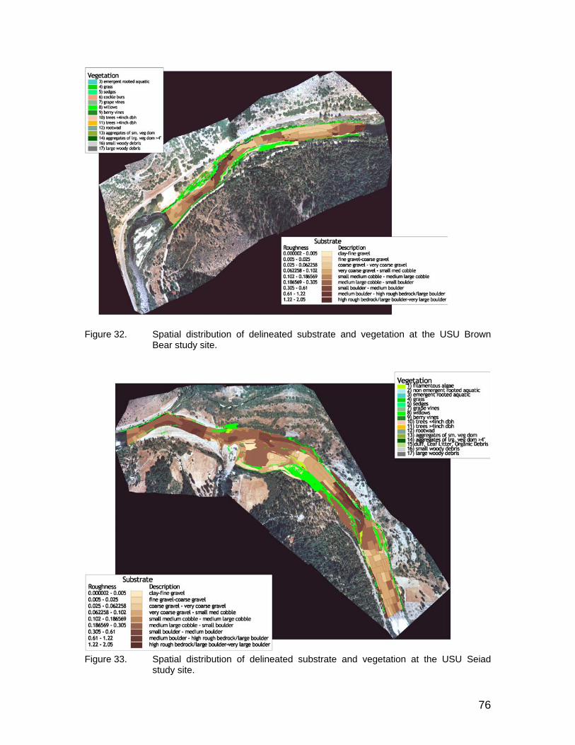
76
Figure 32. Spatial distribution of delineated substrate and vegetation at the USU Brown
Bear study site.
Figure 33. Spatial distribution of delineated substrate and vegetation at the USU Seiad study site.

77
Figure 34. Spatial distribution of delineated substrate and vegetation at the USU Rogers Creek study site.
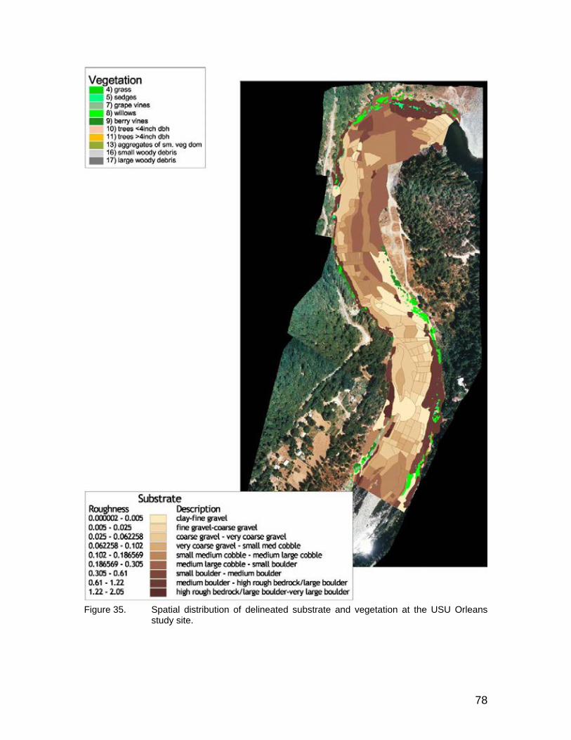
78
Figure 35. Spatial distribution of delineated substrate and vegetation at the USU Orleans
study site.

79
Figure 36. Spatial distribution of delineated substrate and vegetation at the USU Saints Rest Bar study site.
Figure 37. Spatial distribution of delineated substrate and vegetation at the USU Young’s
Bar study site.

80
Stochastic Time Series Modeling for Flows As noted previously in the report, the BOR Natural Flow Study level-pool consumptive use mean monthly flows were utilized to evaluate flow and temperature conditions for the 1963 to 2004 period of record using SIAM. In other analyses, the RMA modeling results for existing conditions or for without project or no project simulations for the 2000 to 2004 period. These sources of results are noted where appropriate. The NAS committee is evaluating the efficacy of the natural flow study results and we will defer to their assessments. We have assumed for the purposes of our modeling that they are generally reflective of the seasonal pattern and flow magnitudes. We recognize that there is a degree of uncertainty in the estimation of the natural flow or consumptive use based modeling results and the implications of using these flows (and others) in the flow recommendation process. The BOR Natural Flow Study results for estimated mean monthly flows at Iron Gate Dam from 1949-2000 were used in SAMS-2000 (Salas et al, 2000) to construct a Periodic Autoregressive Moving Average (PARMA) model. This model was used to generate 1000 synthetic monthly flow traces at Iron Gate Dam based on the underlying statistical characteristics of the estimated flows. PARMA models are popular due to their ability to represent seasonal fluctuations in the mean, standard deviation, and autocorrelation of flows. These models are robust in providing reliable simulations in the expected variation of estimated river flows. Although not part of our scope, we developed this stochastic time series model as a means of addressing the uncertainty in the input flow series from the BOR and providing a means of propagating that uncertainty at least to the calculation of physical habitat. No resources or time were available to link these simulations to either SIAM or RMA models. The basic structure of PARMAS(p,q)model is given the following equation.
∑∑=
−=
− −+=q
jjttt
p
jjttt jXjX
11)()( εθεφ
where p and q determine the order of the PARMA model in the form of lag and S represents the seasons. Xt and Xt-1 are the random variable values at time 't' and 't-1'. tε is the sequence of random variables with zero mean and a standard deviation of 1.0 and represent the residuals. Where as tφ and tθ respectively are the autoregressive and moving average parameters. Further details on formulation, parameterization, and analysis of PARMA models can be found in Salas (1993) and Tesfaye et al., (2006). In the current application, a seasonal PARMA12(5,0) model was fitted to the data.
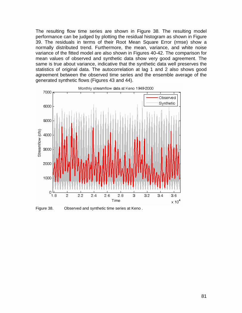
81
The resulting flow time series are shown in Figure 38. The resulting model performance can be judged by plotting the residual histogram as shown in Figure 39. The residuals in terms of their Root Mean Square Error (rmse) show a normally distributed trend. Furthermore, the mean, variance, and white noise variance of the fitted model are also shown in Figures 40-42. The comparison for mean values of observed and synthetic data show very good agreement. The same is true about variance, indicative that the synthetic data well preserves the statistics of original data. The autocorrelation at lag 1 and 2 also shows good agreement between the observed time series and the ensemble average of the generated synthetic flows (Figures 43 and 44).
Figure 38. Observed and synthetic time series at Keno .
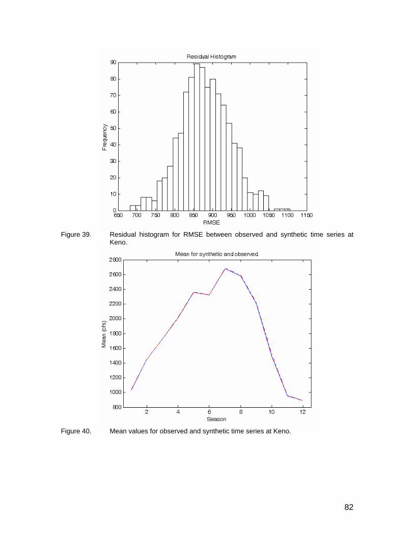
82
Figure 39. Residual histogram for RMSE between observed and synthetic time series at
Keno.
Figure 40. Mean values for observed and synthetic time series at Keno.

83
Figure 41. Variance values for observed and synthetic time series at Keno.
Figure 42. White noise variance for fitted model.
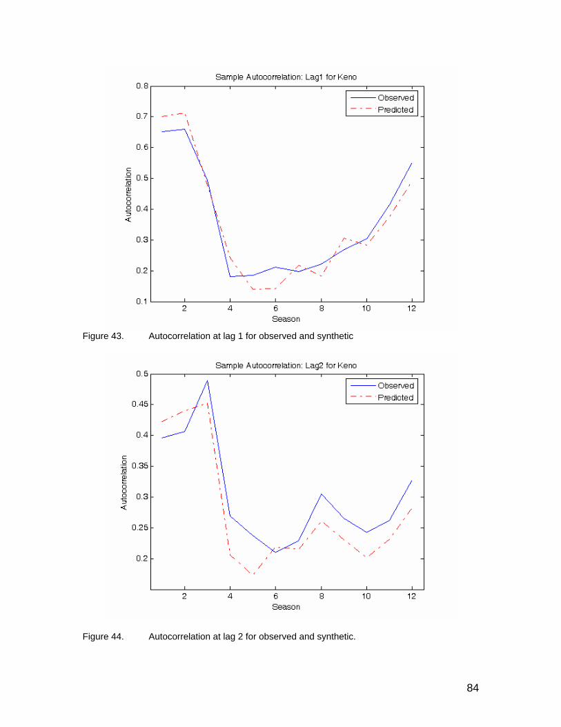
84
Figure 43. Autocorrelation at lag 1 for observed and synthetic
Figure 44. Autocorrelation at lag 2 for observed and synthetic.

85
The simulation results were utilized to estimate the expected variance in flow on a monthly basis over a range of exceedence levels. An example based on August at Keno is provided in Figure 45 and is illustrative of results in other months, which are provided in Appendix D.
Figure 45. Ensemble range in simulated monthly flows at Iron Gate Dam over different
exceedence levels. We believe the stochastic PARA model is biased in that it underpredicts the magnitude of the mean flows associated with exceedences greater than about 75 percent in most months (see Appendix D). Interestingly, when we fitted a multivariate seasonal model to the estimated natural flows at Keno, Shasta, Scott, Salmon, and Trinity for this same period of record the ensemble averages for all months were approximately 100 to 200 cfs higher than the BOR flows at Keno. Although we could not peruse this type of stochastic modeling for this report, we recommend that it be considered in future evaluations. We believe that linking up the spatial and temporal characteristics of at least the major tributaries would broaden insight to the spatial and temporal variations in flow and temperature expected within the main stem Klamath River. We are primarily interested in finding the expected variation rather than the accuracy of estimated mean flows. The stochastic simulation results would indicate that the flow variation between the 1st and 3rd quartiles are within about 10 to 15 percent of the monthly mean flow at a given exceedence level. However, we have confined the use of these results to the estimation of the uncertainty in the hydrologic regime in terms of expected ranges about the mean
August: Flow Duration Curve at Keno
0
400
800
1200
1600
2000
0 10 20 30 40 50 60 70 80 90 100Exceedence, %
Flow
, cfs
BOR Nat. Flow Stochastic: Mean Stochastic: 1st and 3rd Quartiles

86
and to examine how this range affects estimation of physical habitat. This subject is treated further in the section on Habitat Time Series Modeling below. Hydraulic Modeling Hydraulic modeling was accomplished using a 2-dimensional, quasi-3-dimensional model formulation that was developed and used extensively for research on rivers by Jonathan Nelson of the USGS (Nelson 1996, Thompson et al., 1998, Nelson et al., 1995, McLean et al., 1999, Topping et al., 2000). The model relies on 3-dimensional riverbed topography, flow rate, and stage (i.e., water surface elevations) boundary conditions to calculate flow, velocities, water surface elevations and boundary shear stresses in the channel. It has been used in channels with or without islands in both high and low Froude number flows (i.e., sub-critical and super-critical flow conditions). The model solves the two-dimensional vertically averaged flow equations on an orthogonal curvilinear grid. It uses a spatially variable, scalar kinematic eddy viscosity turbulence closure that emphasizes vertical diffusion of momentum. The program was written to accommodate spatially variable channel roughness and was further modified at USU to enhance the wetting-drying algorithm and initial condition capabilities. These modifications were made to enhance computational efficiency during the iterative process of model calibration and improve overall simulation results. The technical description of this model and underlying equations can be found in the citations noted above. Development of Computational Meshes The DTM generated from the spatial delineation of the study reach described above was used to create a curvilinear orthogonal mesh for the hydrodynamics and habitat modeling. The meshes were generated at each of the study sites using a smooth (gradually varying radius) stream centerline overlaid on the DTM. Hydrodynamic meshes were refined (i.e., number of mesh elements (nodes) and spacing between nodes) of each mesh as much as practical given the size of the intensive study sites and limitations associated with hydrodynamic model computational time requirements. The habitat modeling meshes were refined based on the minimum distance needed for the habitat modeling (e.g., minimum distance to cover). For this study, the computational meshes used in the hydraulic simulations at all sites contained nodes every 1.6 meters (5.25 feet) across the river and 1.7 meters (5.58 feet) in the longitudinal direction (i.e., up and down the river). An example of the computational mesh for the RRanch study site is illustrated in Figure 46. The hydraulic solutions at this mesh density were subsequently used to interpolate the hydraulic attributes on a 0.61meter (~ 2.0 feet) habitat modeling meshes for use in habitat modeling as described below.

87
Figure 46. Example of the hydrodynamics computational mesh at RRanch used in the
hydrodynamic modeling of water surface elevations and velocities at USU study sites.
Water Surface Modeling At each intensive study site, three sets of measured water surfaces and calibration discharges were surveyed (see Table 10) for use in calibration of the hydrodynamic model. The two-dimensional hydraulic model at each site was calibrated to measured water surfaces by adjusting roughness for each computational node. This calibration was facilitated from the overlays of the delineated substrate and vegetation polygons onto the computational meshes at each site as described previously (see Figures 30 through 37). For each substrate or vegetation type, we associated an estimated hydraulic roughness height based on the size of the particle size (or largest particle size when mixed substrates were delineated) or vegetation type in each substrate/vegetation category. In the case of substrates, the hydraulic roughness was based on a drag coefficient calculated from the roughness length (particle size) of each substrate category. In the case of vegetation, roughness was assigned according the morphometry and density of the vegetation delineated within a polygon (e.g., grass versus willows). Roughness values were assigned from published values in the literature for vegetation (Chow 1959, Arcement and Schneider 1989). The roughness associated with vegetation and substrate classes are provided in Table 12. An example of these assignments spatially within the USU RRanch study site is illustrated in Figure 47.

88
Table 12. Hydraulic roughness assigned to classes of vegetation used in the 2-dimensional hydrodynamic modeling at USU study sites.
Figure 47. Example of spatially explicit assignment of variable roughness for different
substrate and vegetation codes within the USU RRanch study site (vegetation roughness is in green and substrate roughness is in red).
Vegetation CodesRoughness Sparse (s) and Dense (d)
Hydrodynamic Roughness
Code Approximate Mannings nFilamentous Algae low (d&s) 500/500 High= 0.15Non Emergent Rooted Aquatic low (d&s) 500/500 Med High=0.10Emergent Rooted Aquatic high (d), med high (s) 900/800 Med=0.06Grass med (d), low (s) 700/500 Low=0.035Sedges med (d), low (s) 700/500Cockle Burs med (d), low (s) 700/500Grape Vines high (d), med (s) 900/700Willows high (d), med (s) 900/700Berry Vines high (d), med (s) 900/700Trees <4" dbh med high (d), med (s) 800/700Trees >4" dbh med high (d), med (s) 800/700Rootwad high (d), med (s) 900Aggregates of Small Veg Dom (<4") high (d), med (s) 900/700Aggregates of Small Veg Dom (>4") high (d), med (s) 900/700Duff, Leaf Litter, Organic Debris Typically use substrateSmall Woody Debris (SWD) <4"x12" high (d), med (s) 700Large Woody Debris (LWD) >4"x12" high (d), med (s) 900

89
This process assigned differential roughness spatially across all computational nodes as an initial starting point in the model calibration process. During the calibration phase of the hydrodynamics modeling, the roughness height assigned to specific nodes for substrate was increased or decreased by a constant percentage globally until the modeled water surface matched the measured water surface at that calibration flow. This was first undertaken at the high calibration flow. The calibrated roughness was then used in subsequent simulations to verify model performance at the medium and low calibration flows. When a channel roughness height adjustment was obtained throughout the study site that generated accurate water surface elevation predictions at all calibration flows, the hydrodynamics model was assumed to be calibrated. All subsequent hydraulic simulations for various flows used in the habitat modeling were modeled with these same calibrated channel roughness heights. Water surface modeling results were generally within 1 to 5 centimeters over the entire spatial domain of each study site. This is illustrated for the results at the USU RRanch study site in Figure 48. This figure shows the difference between measured and modeled water surface elevations at a flow rate of 157 cubic meters per second (~ 5,544 cfs). Appendix E contains plots of observed versus modeled water surface elevations at all calibration flows for all study sites.
Figure 48. Difference between measured and modeled water surface elevations at the USU
RRanch study site at a flow rate of 157 cubic meters per second (~5,544 cfs). Note the legend is in meters.

90
In some instances, because the measured water surfaces were based on point measurements along the margins of the stream (linear water surface created using a TIN) and the modeled waters surfaces were computed everywhere in the channel, there were some apparent differences between measured and modeled water surfaces in the middle of the channel that were simply an artifact of the comparison methodology. In general, only the differences along the margins of the channel are real differences. Bhosle (2004) examined the difference between predicted and observed depths (water surface elevation minus bed topography) at 18 study sites within the Nooksack River Basin, Washington based on the hydrodynamic model used in this study. Table 13 shows the mean annual flow, measured calibration discharges, and the number of points utilized in the assessment of modeling errors. Table 13. Study site mean annual flow, measured calibration discharges, and number of
points used for the assessment of depth and velocity modeling errors.
Study Sites Mean Annual Flow (cms)
Calibration Flows (cms)
Number of Nodes where velocity and depth points collected
Whatcom Creek 2.24 0.52 2.82 4.47 171234 Bertrand Creek 0.84 0.09 0.21 0.5 73738 Fishtrap Creek 0.92 0.21 0.4 1.23 12717 Ten Mile Creek 1 0.22 0.48 1.16 49266
Anderson Creek – Lower 0.33 0.03 0.18 0.38 42612 Anderson Creek – Upper 0.33 0.03 0.18 0.38 13608
Middle Fork Nooksack River 18.17 9.26 14.39 23 227447 Main stem Nooksack River near Ferndale 111.22 66.31 81.84 86.08 88641 Main stem Nooksack River near Everson 102.39 49.3 82.16 103.12 152625
Main stem Nooksack River near Demming 96.07 37.38 75.32 171.32 45904 Kendal Creek – Lower 1.09 0.01 0.1 1.21 31725 Kendal Creek – Upper 1.09 0.01 0.1 1.21 48242
Maple Creek 1.15 0.25 0.61 1.29 74385 South Fork Nooksack River – Upper 24.91 7.6 17.41 25.46 140850
Hutchison Creek 1.19 0.3 0.67 2.32 48013 Austin Creek – Lower 0.54 0.05 0.21 1.85 65527 Austin Creek – Upper 0.54 0.05 0.21 1.85 88641
Figure 49 shows the frequency distribution of measured versus modeled water depths derived from the spatial distribution of predicted water surface elevations at measured points. As this figure illustrates, the errors in modeled depths are approximately normally distributed with a mean of 0.002 meters and a variance of 0.001.
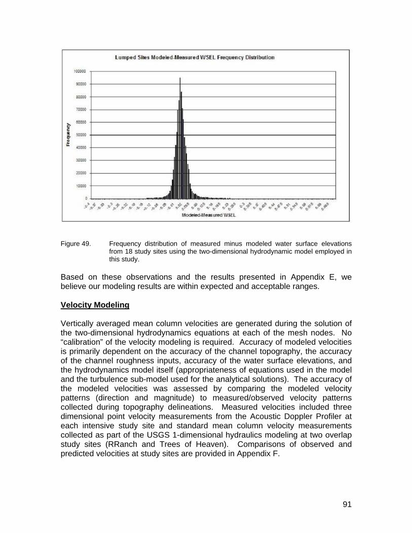
91
Figure 49. Frequency distribution of measured minus modeled water surface elevations
from 18 study sites using the two-dimensional hydrodynamic model employed in this study.
Based on these observations and the results presented in Appendix E, we believe our modeling results are within expected and acceptable ranges. Velocity Modeling Vertically averaged mean column velocities are generated during the solution of the two-dimensional hydrodynamics equations at each of the mesh nodes. No “calibration” of the velocity modeling is required. Accuracy of modeled velocities is primarily dependent on the accuracy of the channel topography, the accuracy of the channel roughness inputs, accuracy of the water surface elevations, and the hydrodynamics model itself (appropriateness of equations used in the model and the turbulence sub-model used for the analytical solutions). The accuracy of the modeled velocities was assessed by comparing the modeled velocity patterns (direction and magnitude) to measured/observed velocity patterns collected during topography delineations. Measured velocities included three dimensional point velocity measurements from the Acoustic Doppler Profiler at each intensive study site and standard mean column velocity measurements collected as part of the USGS 1-dimensional hydraulics modeling at two overlap study sites (RRanch and Trees of Heaven). Comparisons of observed and predicted velocities at study sites are provided in Appendix F.

92
Bhosle (2004) also examined the difference between predicted and observed velocities at the 18 study sites listed in Table 13. Figure 50 shows the frequency distribution of measured versus modeled velocities. As this figure illustrates, the errors in modeled velocities are approximately normally distributed with a mean of 0.012 m/s and a variance of 0.013.
Figure 50. Frequency distribution of measured minus modeled velocities from 18 study sites
using the two-dimensional hydrodynamic model employed in this study. Based on these observations and the results presented in Appendix F, we believe our modeling results are within expected and acceptable ranges for the application of this class of hydrodynamic model. QA/QC evaluations conducted by USU at the Young’s Bar study site indicated that modeling solutions were unacceptable. Our technical assessment indicated that the upstream boundary of the study site (see Figure 27) was being impacted by the large gravel bar that extended above the study site boundary. At different flow rates, water partitions between the main channel and a side channel on the left side of the bar (see lower right area in Figure 27). Insufficient channel topography existed to extend the study site upstream and insufficient data existed to allow an accurate partitioning of the flows into the top of the modeled reach. Based on these results, the Young’s Bar study site was dropped from the assessments.
93
Ranges of Simulated Flows The ranges of simulated flows for the models were based on the quality of the simulations and range of target flows desired for the assessments. Flow ranges between 400 and 8,000 cfs at stations in the river reach immediately below Iron Gate Dam are within what would be considered valid ranges for application of these modeling tools based on the measured calibration discharges and hydraulic modeling calibration and simulation results (Bovee 1995, Hardy 2000). For study sites in successive river reaches below Iron Gate Dam, the calibration data reflects increased flows associated with tributary accretions, and therefore, the range of simulated discharges increase proportionally. For example, at the Saints Rest Bar study site, the lower range of simulated flows is approximately 2200 cfs and the upper range is approximately 19,500 cfs. In all cases, the valid ranges of simulated flows generally encompass the expected monthly flow ranges for the main stem Klamath River germane to the assessment of instream flow recommendations. In some cases, however, especially at very low exceedence ranges (i.e., high flows), flow rates were higher than the simulated ranges for the hydraulics. This is addressed where appropriate in the development of the instream flow recommendations. Fish Habitat Utilization Fish habitat utilization data were collected to meet two critical study objectives. The first objective was to provide data suitable for development and testing of the conceptual physical habitat models for target species/life stages and subsequent validation of the habitat modeling results. The second objective was to obtain sufficient data to develop site-specific suitability criteria for use in the habitat models. Fisheries collection data at intensive study sites involved a number of sampling protocols depending on the species/life stage and specific objective(s). Redd survey data were obtained from either the USFWS or Tribal collaborators. These data included species, spatial location if within a study site, substrate type, depth, and velocity. Other data were collected but not utilized in the assessments. Data for other life stages were provided by CDFG, USFWS, and Tribal sources. The number of samples taken and number of sampling efforts over time varied between study sites as noted below. Life stages of fry and juveniles were sampled through a combination of gear types including direct observations, seining, and electrofishing. Each sampling location (or redd count) was located either using GPS or standard surveying equipment. When standard surveying was undertaken, the survey was tied to the control network at the study site. Available collection data were registered to the orthophotographs in GIS for Habitat Modeling and HSC validation as discussed later in the report.

94
Data collected specifically for use in the development of HSC also included collection of physical attributes such as depth, velocity, substrate, cover, and distance to cover for non-spawning life stages. This work was undertaken as part of ongoing study efforts by the USGS/USFWS, HSC development work contracted by the CDFG, with assistance from Tribal Fisheries Program personnel. Field collection efforts specifically targeted collection of fish location data to validate the habitat modeling results at USU study sites. Selection of Target Species and Life Stages for Phase II Evaluations Due to the limitations of availability of site-specific or literature based HSC for all native species and life stages within the main stem Klamath River only specific species and life stages were included for quantitative analyses in Phase II. The specific species and life stages included in the Phase II analyses are listed in Table 14. Table 14. Species and life stages used in quantitative assessments of instream flow
requirements for the main stem Klamath River.
Species Life Stages Steelhead Fry and 1+ (Juveniles) Chinook Spawning, Fry, and Juvenile Coho Fry and Juvenile
This list of species and life stages were derived from extensive discussions with the Technical Team. The selection of these species and life stages were made after reviewing simulation results using both site-specific and literature based HSC developed for the study. In addition, although some species and life stages were considered for inclusion based on available HSC in the literature (e.g., sturgeon), these curves were not considered appropriate for application to the Klamath River and therefore were not included in the analyses. NRC (2004) note that the main stem is ‘not as important’ as the tributaries for spawning and rearing for coho and that the main stem is generally avoided in the July through September period. They also note the importance of the main stem for Chinook and steelhead fry/juvenile life stages during this same period. We believe coho restoration efforts in tributary systems are critical for that species and these efforts will inherently benefit all aquatic species within the main stem Klamath River. However, it is important to note that that coho spawning is observed in the main stem Klamath River such as in 2004 at locations similar to surveys conducted in 2001. In 2004, redds were located in the main channel, split channel, and side channel areas of the main stem Klamath River, with the majority located between Iron Gate Dam and the Scott River. Coho fry have also been captured in Chinook out-migrant sampling efforts in the main stem Klamath River located below Bogus Creek, the I-5 Bridge, and above the Scott River
95
confluence. In 2002, over 4,000 fry were captured at these three locations. Based on juvenile Chinook sampling efficiencies, it is estimated that a total of over 1.2 million coho fry passed these three combined trapping locations (Tom Shaw, USFWS unpublished data). Even if the trapping efficiencies are significantly biased, there is still a large number of coho utilizing the main stem seasonally within the Klamath River. Stutzer et al., (2006) found that downstream migrating wild coho smolts held in main stem habitats between 1 and 37 days while hatchery tagged smolts held in main stem habitats between 2 and 30 days. Furthermore they report that their mobile and habitat use data collected during 2005 suggest that juvenile coho used the upper main stem Klamath River for rearing for significant periods. Based on these empirical observations, coho fry and juvenile life stages were considered in all months for which known use were documented. Species and Life Stage Periodicities Hardy (1999) provided an interim species and life stage periodicity for the anadromous species within the main stem Klamath River. The Technical Team reviewed existing fisheries collection data from the Klamath River and additional literature on known or suspected species distributions and life stage periodicities. This review included consideration of potential longitudinal and seasonal variation within the main stem Klamath River between Iron Gate Dam and the estuary. The revised species periodicity by reach segment was derived from this compiled information and input from the Technical Team. It is recognized that potential refinement of this information will continue as part of the long-term instream flow study being conducted by the USFWS and other collaborators. The species and life stage periodicity used in the assessment of instream flows is provided in Table 15.11 Monthly Species and Life Stage Critical Factors Related to Flows Table 16 provides a synopsis of critical life history needs associated with different species and life stages within the main stem Klamath River. This information supplements the basic periodicity data shown in Table 15 and provides the context of species/life stage needs necessary to be considered when evaluating instream flow needs.
11 Comments from Klamath Water Users Association takes issues with the ‘broad’ nature of the species periodicity used in our assessments. We disagree with this comment given known intra-annual variation in flows/temperature, known shifts in run timing of several weeks over the past 50 years, and unknown influence of long-term climate change that may further impact the timing of upstream and downstream migration. Our approach is conservative in this regard.
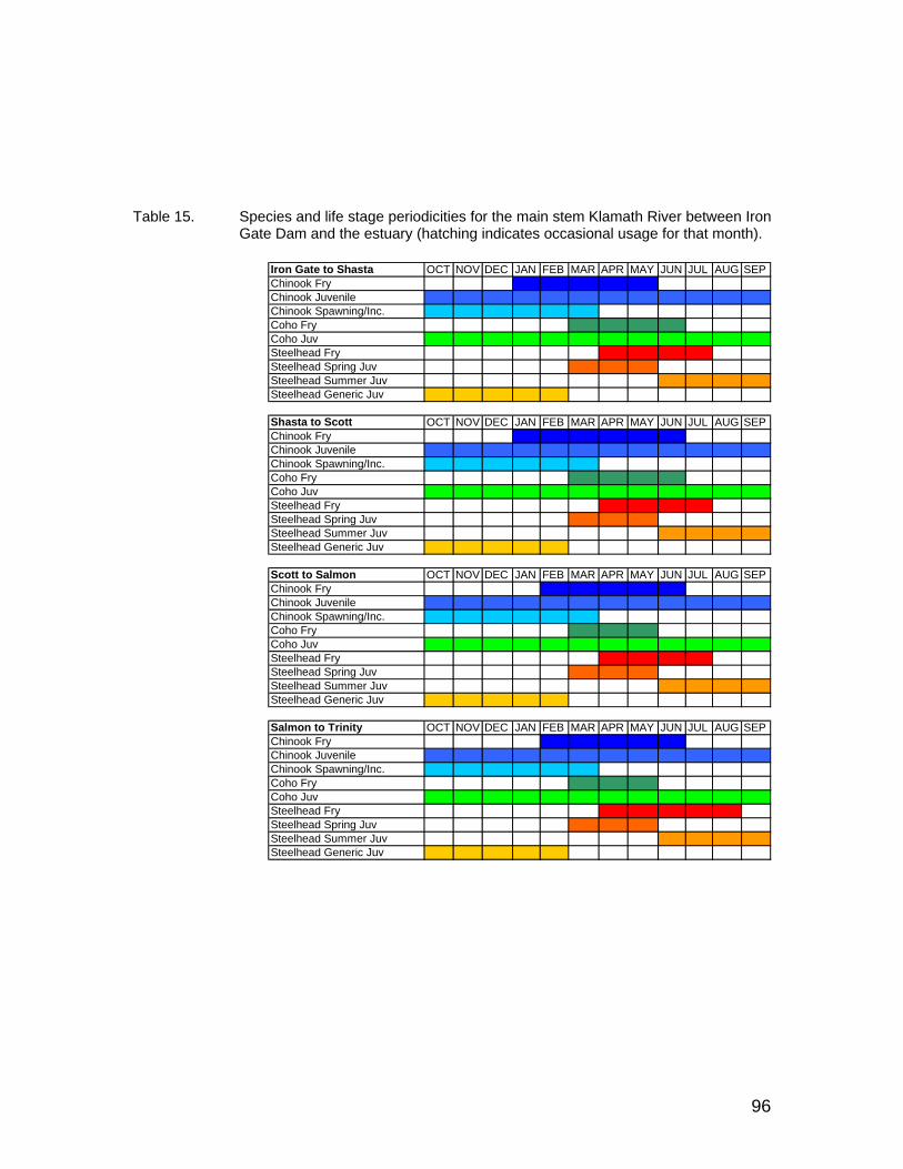
96
Table 15. Species and life stage periodicities for the main stem Klamath River between Iron
Gate Dam and the estuary (hatching indicates occasional usage for that month).
Iron Gate to Shasta OCT NOV DEC JAN FEB MAR APR MAY JUN JUL AUG SEPChinook Fry Chinook Juvenile Chinook Spawning/Inc. Coho Fry Coho JuvSteelhead Fry Steelhead Spring Juv Steelhead Summer Juv Steelhead Generic Juv
Shasta to Scott OCT NOV DEC JAN FEB MAR APR MAY JUN JUL AUG SEPChinook Fry Chinook Juvenile Chinook Spawning/Inc. Coho Fry Coho JuvSteelhead Fry Steelhead Spring Juv Steelhead Summer Juv Steelhead Generic Juv
Scott to Salmon OCT NOV DEC JAN FEB MAR APR MAY JUN JUL AUG SEPChinook Fry Chinook Juvenile Chinook Spawning/Inc. Coho Fry Coho JuvSteelhead Fry Steelhead Spring Juv Steelhead Summer Juv Steelhead Generic Juv
Salmon to Trinity OCT NOV DEC JAN FEB MAR APR MAY JUN JUL AUG SEPChinook Fry Chinook Juvenile Chinook Spawning/Inc. Coho Fry Coho JuvSteelhead Fry Steelhead Spring Juv Steelhead Summer Juv Steelhead Generic Juv
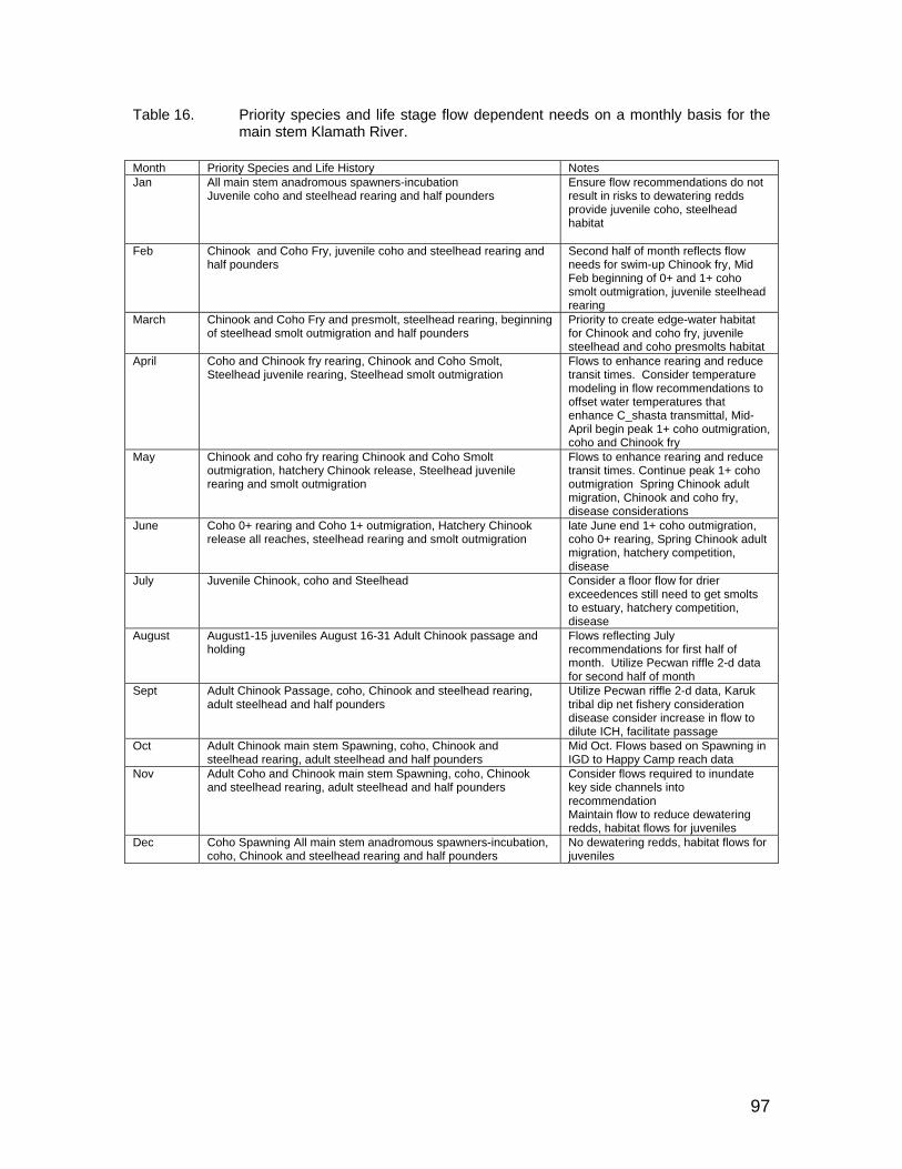
97
Table 16. Priority species and life stage flow dependent needs on a monthly basis for the main stem Klamath River.
Month Priority Species and Life History Notes Jan All main stem anadromous spawners-incubation
Juvenile coho and steelhead rearing and half pounders
Ensure flow recommendations do not result in risks to dewatering redds provide juvenile coho, steelhead habitat
Feb Chinook and Coho Fry, juvenile coho and steelhead rearing and half pounders
Second half of month reflects flow needs for swim-up Chinook fry, Mid Feb beginning of 0+ and 1+ coho smolt outmigration, juvenile steelhead rearing
March Chinook and Coho Fry and presmolt, steelhead rearing, beginning of steelhead smolt outmigration and half pounders
Priority to create edge-water habitat for Chinook and coho fry, juvenile steelhead and coho presmolts habitat
April Coho and Chinook fry rearing, Chinook and Coho Smolt, Steelhead juvenile rearing, Steelhead smolt outmigration
Flows to enhance rearing and reduce transit times. Consider temperature modeling in flow recommendations to offset water temperatures that enhance C_shasta transmittal, Mid- April begin peak 1+ coho outmigration, coho and Chinook fry
May Chinook and coho fry rearing Chinook and Coho Smolt outmigration, hatchery Chinook release, Steelhead juvenile rearing and smolt outmigration
Flows to enhance rearing and reduce transit times. Continue peak 1+ coho outmigration Spring Chinook adult migration, Chinook and coho fry, disease considerations
June Coho 0+ rearing and Coho 1+ outmigration, Hatchery Chinook release all reaches, steelhead rearing and smolt outmigration
late June end 1+ coho outmigration, coho 0+ rearing, Spring Chinook adult migration, hatchery competition, disease
July Juvenile Chinook, coho and Steelhead Consider a floor flow for drier exceedences still need to get smolts to estuary, hatchery competition, disease
August August1-15 juveniles August 16-31 Adult Chinook passage and holding
Flows reflecting July recommendations for first half of month. Utilize Pecwan riffle 2-d data for second half of month
Sept Adult Chinook Passage, coho, Chinook and steelhead rearing, adult steelhead and half pounders
Utilize Pecwan riffle 2-d data, Karuk tribal dip net fishery consideration disease consider increase in flow to dilute ICH, facilitate passage
Oct Adult Chinook main stem Spawning, coho, Chinook and steelhead rearing, adult steelhead and half pounders
Mid Oct. Flows based on Spawning in IGD to Happy Camp reach data
Nov Adult Coho and Chinook main stem Spawning, coho, Chinook and steelhead rearing, adult steelhead and half pounders
Consider flows required to inundate key side channels into recommendation Maintain flow to reduce dewatering redds, habitat flows for juveniles
Dec Coho Spawning All main stem anadromous spawners-incubation, coho, Chinook and steelhead rearing and half pounders
No dewatering redds, habitat flows for juveniles
98
The Ecological Basis of Habitat Suitability Criteria (i.e. Niche Theory) In general, it is commonly believed that it is most appropriate to develop site-specific HSC data from the river in which the instream flow assessment is undertaken. However, many factors such as under seeding, presence of predators, presence of introduced species, modified habitat, etc., can make development of HSC from the target stream system both infeasible and/or undesirable. Furthermore, poor field conditions (e.g., low water visibility) can also make collection of HSC data infeasible in many river systems on a seasonal basis. When site specific HSC cannot be developed then the next approach taken is to assess the applicability of HSC from another river. This should include observational data for target species and life stages in the stream under study in order to attempt a validation or transferability test of the HSC. Existing methods for testing applicability (transferability) of HSC (e.g., Thomas and Bovee 1993) are not widely accepted and are known to produce inconsistent results (Dunbar and Ibbotson 2001). Finally, in the absence of transferable HSC, literature based curves in conjunction with professional judgment by species experts are most often utilized to select HSC in applied instream flow assessments. This is the most commonly applied technique for HSC ‘development’ for instream flow assessments in the U.S. and internationally. In order to understand the distribution and abundance of a species it is necessary to know several things:
• The life history requirements of the species, • The resources that it requires (e.g., food, space), • The effects of environmental conditions (e.g., velocity, temperature), • The rates of birth, death, and migration, and the • Interactions with their own and other species (competition and predation).
One of the fundamental concepts that have helped ecologists understand the distribution and abundance of species is the ecological niche (Hutchinson 1957; Schoener 1988). The ecological niche is the set of environmental conditions (e.g., temperature, depth, velocity) and resources (things that are consumed such as food) that are required by a species to exist and persist in a given location. There are many environmental conditions and resources that make up a niche. Typically, each condition and resource is thought of as a dimension of the niche. Along an individual dimension of a niche (e.g., temperature) there is a range of values of the condition or resource that is suitable for the species. There is also a range that is beyond the ability of the organism to exist. The many individual dimensions of the niche interact to create a multidimensional “niche volume” of conditions and resources that provide a suitable environment for a species (e.g., temperature, velocity, depth, food). This environment of suitable conditions and resources has been defined as the fundamental niche of a species.

99
The fundamental niche of a species must exist in a location both temporally and spatially for a species to occupy that location. Whether or not a species actually occupies a location, however, also depends on whether or not the species has access to the location and whether or not it is precluded from occupying the location by other species because of competition or predation. The portion of a species fundamental niche that a species actually occupies is called its realized niche. The realized niche varies depending on the number, types, and effectiveness of competitors and predators. The realized niche also depends on availability and variability of conditions and resources in the environment. For riverine fishes, some of the most important niche dimensions are water temperature, hydraulics (interaction of depth and velocity), substrate, cover, and food. Multiple species can coexist in a river by utilizing a combination of niche dimensions differently. If two species utilize the same or nearly the same combination of resources and environmental conditions (niche) at the same time and in the same locations, the potential exists for the more competitive of the two species to exclude the other from the system or from much of its fundamental niche. Likewise, predators can exclude species from occupying much of their fundamental niche through intimidation or predation (Powers 1985; Schlosser 1987; and others). Species and life stage specific HSC as used in instream flow determinations are an attempt to measure the important niche dimensions of a particular species and life stage (Gore and Nestler 1988). These criteria are then used to identify how the amount of space corresponding to the measured niche changes with river discharge. The assumption then, is that there is a positive relationship between the amount of space that exhibits suitable niche conditions and the potential numbers of the species and life stage in the river (Orth and Maughan 1982; Jowett 1992; Nehring and Anderson 1993; and others). In principle, increasing the range, availability, and abundance (diversity) of the important niche dimensions utilized by riverine fishes can increase the number of potential niches that can coexist in a river and can increase the diversity of fish species and life stages in the river. Several investigators have shown that species and life stage diversity in rivers is directly related to the diversity of important niche dimensions (e.g., Gorman and Karr 1978, Schlosser 1987). Diversity of environmental conditions and resources results in biotic diversity (Allan 1995), but only if the spatial and temporal diversity is within a range of conditions to which the species are pre-adapted (only if diversity equates to a diversity of suitable niche conditions). For example, highly variable environmental conditions result in a diverse environment, but low species diversity (Horwitz 1978; Bain et al., 1988) because species are not adapted to the rapidly changing conditions. Several investigators have quantified the range of conditions and resources that various riverine fishes inhabit (Lobb and Orth 1991; Aadland 1993; Bain et al., 1988; Bowen et al., 1998), particularly with

100
respect to depth and velocity. They have identified species and life stage guilds that utilize the niche dimensions of depth and velocity in a similar manner. Guilds typically use a set of environmental conditions or resources similarly, but typically differ in the temporal or spatial use of these resources or differ along other niche dimensions (i.e., food utilization) to coexist. Because stream flow is one of the key factors that controls the temporal and spatial availability of stream hydraulics (interaction of depth and velocity), substrate, cover, food, and to a lesser extent temperature (e.g., Statzner and Higler 1986), stream flow within a given river system controls the abundance and diversity of niche dimensions and the diversity of species that can exist. One method of quantifying the effects of stream flow on riverine biota is to quantify the diversity of habitat types (types inhabited by typical riverine fish guilds) versus flow (e.g., Aadland 1993; Bowen et al., 1998). The diversity of the habitats types, particularly key bottleneck habitats that may affect recruitment of fishes at various times of the year (e.g., spawning or nursery habitat) can be used to identify stream flows that maintain habitats for a diversity of species and life stages (Bain et al., 1988; Scheidegger and Bain 1995; Nehring and Anderson 1993). A particularly useful complement to this method is to individually quantify habitat for important or key species and life stages. Analysis of individual species and life stages has been used for a long time in instream flow assessments. Unfortunately, many of these past assessments looked only at a few individual species and/or life stages. It is important, however, to analyze individual species and life stages in the context of the entire community and ecology of the river (e.g., Orth 1987). Given perfect knowledge of a species and life stage’s realized niche (seasonally and with respect to discharge) in a river system, it would be possible to quantify how the amount of its realized niche changes with flow. This could be used to generate a flow regime that minimizes habitat bottlenecks for target species and life stages. If this analysis was done in concert with a community wide assessment (see above), the flow regime could be generated that did not create undue bottlenecks for other species and life stages in the system. Perfect knowledge of a species and life stage niche is at a practical level unobtainable however, and as a result, approximations of the realized niche must suffice (i.e., HSC). HSC generated from fish observations in a river system are typically used to quantify the realized niche in terms of depth, velocity, substrate, and cover (although most investigators do not recognize them as such). However, generation of HSC is fraught with many difficulties. Some of the most serious of these are logistics constraints that affect the size, timing, and quality of the data sample, habitat availability biases that exist at the time of sampling and predation/competition biases that exist at the time of sampling.

101
HSC development is also complicated due to fish habitat use changes with fish size, season, temperature, activity, habitat availability, presence and abundance of competitors and predators, discharge, and changes between years (Orth 1987; Schrivell 1986; Heggenes 1990; Schirvell 1994; Smith and Li 1983; Bozek and Rahel 1992; Everest and Chapman 1972; Moore and Gregory 1988; Modde and Hardy 1992). These factors underscore the importance of validating the HSC, especially in terms of the habitat modeling results. This is specifically addressed below when reporting on the results of the habitat modeling. Development of Site Specific HSC Site-specific HSC were developed for the main stem Klamath River for Chinook spawning, fry, and juveniles; coho fry; and for steelhead 1+ (juvenile) life stages. The general methodologies for field data collection and data reduction can be found in Hardin et al., (2005). All depth and velocity HSC were developed using nonparametric tolerance limits (Bovee 1986) while substrate/escape cover HSC were fitted using normalized frequencies since their data were categorical. Distance to escape cover for Chinook and coho fry utilized a binary function based on the cumulative frequency of distance to cover. Distance to escape cover for Chinook, coho and steelhead used normalized frequencies over the ranges of distances in which 95 percent of fish were observed. Lack of empirical data from the Klamath River existed for the development of site-specific HSC for coho juveniles or steelhead fry so envelope curves were developed based on existing HSC in the literature (see below). Appendix G provides the tabular coordinates for all HSC while additional habitat modeling parameters for specific life stages are discussed in the section on Physical Habitat Modeling below. Substrate and Vegetation Coding for HSC Substrate and vegetation coding differed slightly between the 1999 and 2000 field assessments. Differences in the coding arose from participation of different study personnel. These differences were rectified into a common classification as shown in Table 17 where the ‘1 to 32’ code system was employed for the HSC and used in the coding of ‘channel index’ values in the habitat simulation models as explained below. Chinook Spawning Chinook spawning HSC for depth, velocity and substrate were derived from field data collections within the main stem Klamath River below Iron Gate Dam downstream to the confluence with the Scott River during 1998 and 1999. Tim Hardin and Associates collected these data at approximately 1,200 (mid- to late-October) and 1,800 cfs (early November) as part of California Department of Fish and Game’s on-going contributions to the instream flow assessments within the Klamath River. The study team sampled the river from below Iron Gate Dam to the Scott River during each sample period. The HSC curves were developed

102
from 290 observations taken at identified redd locations. The final HSC values for velocity, depth, and substrate are proved in Figures 51 to 53. Table 17. Substrate and vegetation coding scheme used for all HSC. Year 1999 substrate and vegetation codes
Year 2000 substrate and vegetation codes
Year 1999 substrate and vegetation codes
Year 2000 substrate and vegetation codes
Code Code Description Code Code Description
1 1 Filamentous algae 8 17 Large woody debris (LWD)>4"x12"
2 2 Non emergent rooted aquatic 12 18 Clay
3 3 Emergent rooted aquatic 12 19 S and and/or silt (<0.1")
4 4 Grass 12 20 Coarse sand (0.1-0.2")
4 5 Sedges 13 21 Small gravel (0.2-1")
4 6 Cockle burs 14 22 Medium gravel (1-2")
6 7 Grape vines 15 23 Large gravel (2-3")
6 8 Willows 16 24 Very large gravel (3-4")
6 9 Berry vines 16 25 Small cobble (4-6")
5 10 Trees <4" 17 26 Medium cobble (6-9")
5 11 Trees >4" 18 27 Large cobble (9-12")
10 12 Root wad 19 28 Small boulder (12-24")
11 13 Aggregates of small vegetation dominate <4" 20 29 Medium boulder (24-48")
11 14 Aggregates of large vegetation dominate >4" 21 30 Large boulder (>48")
7 15 Duff, leaf litter, organic debris 22 31 Bedrock-smooth
9 16 Small woody debris (SWD) <4"x12" 22 32 Bedrock-rough
Figure 51. Frequency distribution and HSC values for Chinook spawning for velocity from
the Klamath River.
Chinook Spawning Velocity Suitabilty
0
0.1
0.2
0.3
0.4
0.5
0.6
0.7
0.8
0.9
1
0.0 0.3 0.7 1.1 1.5 1.9 2.3 2.7 3.1 3.5 3.9 4.3 4.7 5.1 5.5 5.9
Velocity (ft/s)
Suita
bilit
y In
dex
0
5
10
15
20
25
30
35
40
Freq
uenc
y

103
Figure 52. Frequency distribution and HSC values for Chinook spawning for depth from the
Klamath River.
Figure 53. Frequency distribution and HSC values or Chinook spawning for substrate from the Klamath River.
Chinook Spawning
0
0.1
0.2
0.3
0.4
0.5
0.6
0.7
0.8
0.9
1
Filamentous A
lgae
Non-em
ergent Rooted A
quatic
Em
ergent Rooted A
quatic
Grass
Sedges
Cockle B
urs
Grape V
ines
Willow
s
Berry V
ines
Trees < 4" dbh
Trees > 4" dbh
Rootw
ad
Aggregates of sm
all veg. dom (<4")
Aggregates of large veg. dom
(<4")
Duff, Leaf Litter, O
rganic Debris
Sm
all Woody D
ebris < 4' x 12'
Large Woody D
ebris > 4' x 12'
Clay
Sand or S
ilt
Coarse S
and
Sm
all Gravel
Medium
Gravel
Large Gravel
Very Large G
ravel
Sm
all Cobble
Medium
Cobble
Large Cobble
Sm
all Boulder
Medium
Boulder
Large Boulder
Sm
ooth Bedrock
Rough B
edrock
Substrate and Vegetation
Suita
bilit
y In
dex
Chinook Spawning Depth Suitabilty
0
0.1
0.2
0.3
0.4
0.5
0.6
0.7
0.8
0.9
1
0.0 0.3 0.6 0.9 1.3 1.7 2.1 2.5 2.9 3.3 3.7 4.1 4.5 4.9 5.3 5.7 6.0
Depth (ft)
Suita
bilit
y In
dex
0
5
10
15
20
25
30
35
Freq
uenc
y
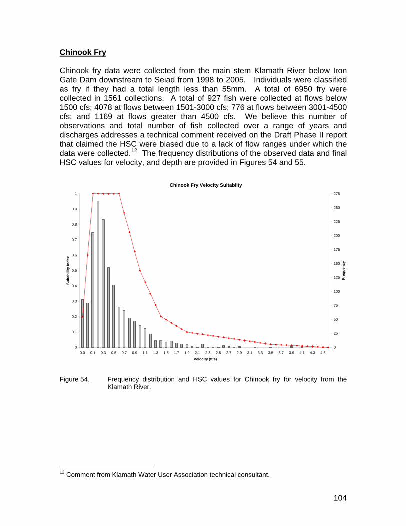
104
Chinook Fry Chinook fry data were collected from the main stem Klamath River below Iron Gate Dam downstream to Seiad from 1998 to 2005. Individuals were classified as fry if they had a total length less than 55mm. A total of 6950 fry were collected in 1561 collections. A total of 927 fish were collected at flows below 1500 cfs; 4078 at flows between 1501-3000 cfs; 776 at flows between 3001-4500 cfs; and 1169 at flows greater than 4500 cfs. We believe this number of observations and total number of fish collected over a range of years and discharges addresses a technical comment received on the Draft Phase II report that claimed the HSC were biased due to a lack of flow ranges under which the data were collected.12 The frequency distributions of the observed data and final HSC values for velocity, and depth are provided in Figures 54 and 55.
Figure 54. Frequency distribution and HSC values for Chinook fry for velocity from the
Klamath River.
12 Comment from Klamath Water User Association technical consultant.
Chinook Fry Velocity Suitabilty
0
0.1
0.2
0.3
0.4
0.5
0.6
0.7
0.8
0.9
1
0.0 0.1 0.3 0.5 0.7 0.9 1.1 1.3 1.5 1.7 1.9 2.1 2.3 2.5 2.7 2.9 3.1 3.3 3.5 3.7 3.9 4.1 4.3 4.5
Velocity (ft/s)
Suita
bilit
y In
dex
0
25
50
75
100
125
150
175
200
225
250
275
Freq
uenc
y

105
Figure 55. Frequency distribution and HSC values for Chinook fry for depth from the
Klamath River. HSC development also included an assessment of Chinook fry habitat use dependent on escape cover type. Figure 56 shows the relationship between Chinook fry and use of substrate and vegetation types delineated from field collections. An assessment was also made to evaluate the spatial relationship between observed fish location and the distance to escape cover derived from the field observations. This is shown in Figure 57.
Chinook Fry Depth Suitabilty
0
0.1
0.2
0.3
0.4
0.5
0.6
0.7
0.8
0.9
1
0.0 0.1 0.3 0.5 0.7 0.9 1.1 1.3 1.5 1.7 1.9 2.1 2.3 2.5 2.7 2.9 3.1 3.3 3.5 3.7 3.9
Depth (ft)
Suita
bilit
y In
dex
0
50
100
150
200
250
300
Freq
uenc
y
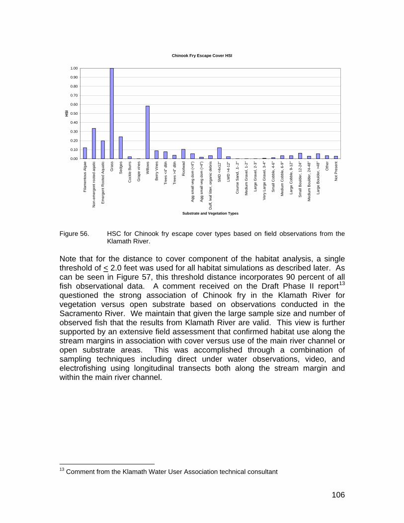
106
Figure 56. HSC for Chinook fry escape cover types based on field observations from the
Klamath River. Note that for the distance to cover component of the habitat analysis, a single threshold of < 2.0 feet was used for all habitat simulations as described later. As can be seen in Figure 57, this threshold distance incorporates 90 percent of all fish observational data. A comment received on the Draft Phase II report13 questioned the strong association of Chinook fry in the Klamath River for vegetation versus open substrate based on observations conducted in the Sacramento River. We maintain that given the large sample size and number of observed fish that the results from Klamath River are valid. This view is further supported by an extensive field assessment that confirmed habitat use along the stream margins in association with cover versus use of the main river channel or open substrate areas. This was accomplished through a combination of sampling techniques including direct under water observations, video, and electrofishing using longitudinal transects both along the stream margin and within the main river channel.
13 Comment from the Klamath Water User Association technical consultant
Chinook Fry Escape Cover HSI
0.00
0.10
0.20
0.30
0.40
0.50
0.60
0.70
0.80
0.90
1.00
Fila
men
tous
Alg
ae
Non
-em
erge
nt ro
oted
aqa
tic
Em
erge
nt R
oote
d A
quat
ic
Gra
ss
Sed
ges
Coc
kle
Burr
s
Gra
pe v
ines
Will
ows
Ber
ry V
ines
Tree
s <4
" dbh
Tree
s >4
" dbh
Roo
twad
Agg
sm
all v
eg d
om (<
4")
Agg
sm
all v
eg d
om (>
4")
Duf
f, le
af li
tter,
orga
nic
debr
is
SM
D <
4x12
"
LWD
>4-
12"
Cou
rse
San
d, .1
-.2"
Med
ium
Gra
vel,
1-2"
Larg
e G
rave
l, 2-
3"
Ver
y La
rge
Gra
vel,
3-4"
Sm
all C
obbl
e, 4
-6"
Med
ium
Cob
ble,
6-9
"
Larg
e C
obbl
e, 9
-12"
Sm
all B
ould
er, 1
2-24
"
Med
ium
Bou
lder
, 24-
48"
Larg
e B
ould
er, >
48"
Oth
er
Not
Pre
sent
Substrate and Vegetation Types
HSI
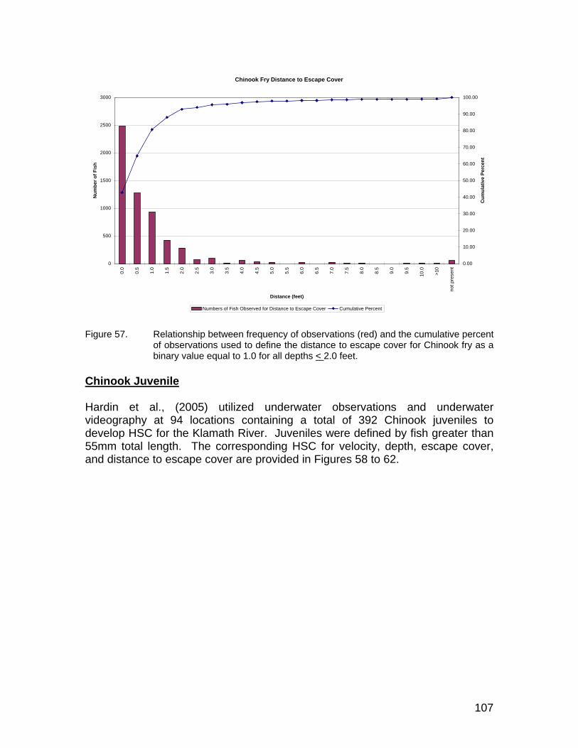
107
Figure 57. Relationship between frequency of observations (red) and the cumulative percent
of observations used to define the distance to escape cover for Chinook fry as a binary value equal to 1.0 for all depths < 2.0 feet.
Chinook Juvenile Hardin et al., (2005) utilized underwater observations and underwater videography at 94 locations containing a total of 392 Chinook juveniles to develop HSC for the Klamath River. Juveniles were defined by fish greater than 55mm total length. The corresponding HSC for velocity, depth, escape cover, and distance to escape cover are provided in Figures 58 to 62.
Chinook Fry Distance to Escape Cover
0
500
1000
1500
2000
2500
3000
0.0
0.5
1.0
1.5
2.0
2.5
3.0
3.5
4.0
4.5
5.0
5.5
6.0
6.5
7.0
7.5
8.0
8.5
9.0
9.5
10.0
>10
not p
rese
nt
Distance (feet)
Num
ber o
f Fis
h
0.00
10.00
20.00
30.00
40.00
50.00
60.00
70.00
80.00
90.00
100.00
Cum
ulat
ive
Perc
ent
Numbers of Fish Observed for Distance to Escape Cover Cumulative Percent

108
Figure 58. Frequency distribution and HSC values for Chinook juveniles for velocity from the
Klamath River.
Figure 59. Frequency distribution and HSC values for Chinook juveniles for depth from the
Klamath River.
Chinook Juvenile Depth Suitabilty
0
0.1
0.2
0.3
0.4
0.5
0.6
0.7
0.8
0.9
1
0.0 0.4 0.8 1.2 1.6 2.0 2.4 2.8 3.2 3.6 4.0 4.4 4.8 5.2 5.6 6.0 6.4 6.8 7.2
Depth (ft)
Suita
bilit
y In
dex
0
5
10
15
20
25
30
35
40
45
Freq
uenc
y
Chinook Juvenile Velocity Suitabilty
0
0.1
0.2
0.3
0.4
0.5
0.6
0.7
0.8
0.9
1
0.0 0.4 0.8 1.2 1.6 2.0 2.4 2.8 3.2 3.6 4.0
Velocity (ft/s)
Suita
bilit
y In
dex
0
10
20
30
40
50
60
70
80
Freq
uenc
y
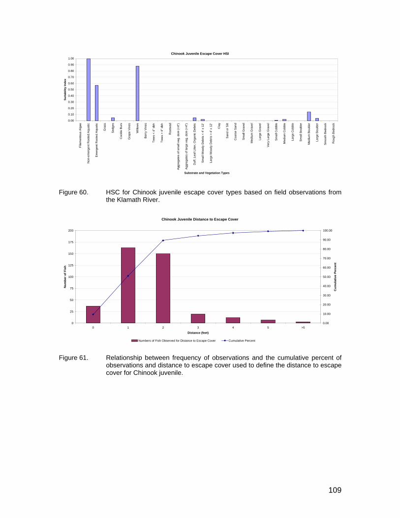
109
Figure 60. HSC for Chinook juvenile escape cover types based on field observations from
the Klamath River.
Figure 61. Relationship between frequency of observations and the cumulative percent of
observations and distance to escape cover used to define the distance to escape cover for Chinook juvenile.
Chinook Juvenile Escape Cover HSI
0.00
0.10
0.20
0.30
0.40
0.50
0.60
0.70
0.80
0.90
1.00
Fila
men
tous
Alg
ae
Non
-em
erge
nt R
oote
d A
quat
ic
Em
erge
nt R
oote
d A
quat
ic
Gra
ss
Sed
ges
Coc
kle
Bur
s
Gra
pe V
ines
Will
ows
Ber
ry V
ines
Tree
s <
4" d
bh
Tree
s >
4" d
bh
Roo
twad
Agg
rega
tes
of s
mal
l veg
. dom
(<4"
)
Agg
rega
tes
of la
rge
veg.
dom
(<4"
)
Duf
f, Le
af L
itter
, Org
anic
Deb
ris
Sm
all W
oody
Deb
ris <
4' x
12'
Larg
e W
oody
Deb
ris >
4' x
12'
Cla
y
San
d or
Silt
Coa
rse
San
d
Sm
all G
rave
l
Med
ium
Gra
vel
Larg
e G
rave
l
Ver
y La
rge
Gra
vel
Sm
all C
obbl
e
Med
ium
Cob
ble
Larg
e C
obbl
e
Sm
all B
ould
er
Med
ium
Bou
lder
Larg
e B
ould
er
Sm
ooth
Bed
rock
Rou
gh B
edro
ck
Substrate and Vegetation Types
Suita
bilit
y In
dex
Chinook Juvenile Distance to Escape Cover
0
25
50
75
100
125
150
175
200
0 1 2 3 4 5 >5
Distance (feet)
Num
ber o
f Fis
h
0.00
10.00
20.00
30.00
40.00
50.00
60.00
70.00
80.00
90.00
100.00
Cum
ulat
ive
Perc
ent
Numbers of Fish Observed for Distance to Escape Cover Cumulative Percent
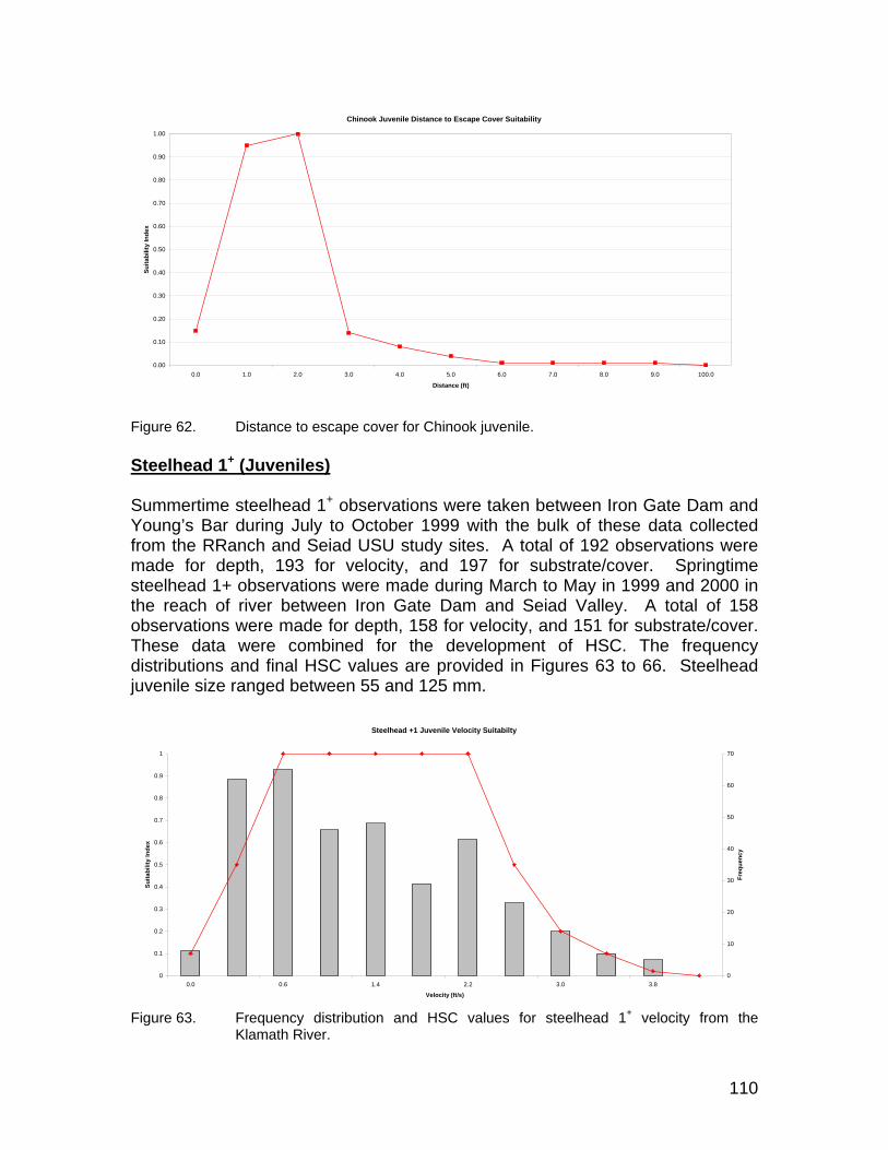
110
Figure 62. Distance to escape cover for Chinook juvenile. Steelhead 1+ (Juveniles) Summertime steelhead 1+ observations were taken between Iron Gate Dam and Young’s Bar during July to October 1999 with the bulk of these data collected from the RRanch and Seiad USU study sites. A total of 192 observations were made for depth, 193 for velocity, and 197 for substrate/cover. Springtime steelhead 1+ observations were made during March to May in 1999 and 2000 in the reach of river between Iron Gate Dam and Seiad Valley. A total of 158 observations were made for depth, 158 for velocity, and 151 for substrate/cover. These data were combined for the development of HSC. The frequency distributions and final HSC values are provided in Figures 63 to 66. Steelhead juvenile size ranged between 55 and 125 mm.
Figure 63. Frequency distribution and HSC values for steelhead 1+ velocity from the Klamath River.
Steelhead +1 Juvenile Velocity Suitabilty
0
0.1
0.2
0.3
0.4
0.5
0.6
0.7
0.8
0.9
1
0.0 0.6 1.4 2.2 3.0 3.8
Velocity (ft/s)
Suita
bilit
y In
dex
0
10
20
30
40
50
60
70
Freq
uenc
y
Chinook Juvenile Distance to Escape Cover Suitability
0.00
0.10
0.20
0.30
0.40
0.50
0.60
0.70
0.80
0.90
1.00
0.0 1.0 2.0 3.0 4.0 5.0 6.0 7.0 8.0 9.0 100.0
Distance (ft)
Suita
bilit
y In
dex

111
Figure 64. Frequency distribution and HSC values for steelhead 1+ depth from the Klamath
River.
Figure 65. Frequency distribution and HSC values for steelhead 1+ escape cover from the
Klamath River.
Steelhead +1 Juvenile Depth Suitabilty
0
0.1
0.2
0.3
0.4
0.5
0.6
0.7
0.8
0.9
1
0.0 0.6 1.4 2.2 3.0 3.8 4.6
Depth (ft)
Suita
bilit
y In
dex
0
10
20
30
40
50
60
70
80
90
Freq
uenc
y
Steelhead +1 Escape Cover HSI
0.00
0.10
0.20
0.30
0.40
0.50
0.60
0.70
0.80
0.90
1.00
Fila
men
tous
Alg
ae
Non
-em
erge
nt R
oote
d Aq
uatic
Emer
gent
Roo
ted
Aqua
tic
Gra
ss
Sedg
es
Coc
kle
Burs
Gra
pe V
ines
Willo
ws
Berry
Vin
es
Tree
s <
4" d
bh
Tree
s >
4" d
bh
Roo
twad
Aggr
egat
es o
f sm
all v
eg. d
om (<
4")
Aggr
egat
es o
f lar
ge v
eg. d
om (<
4")
Duf
f, Le
af L
itter
, Org
anic
Deb
ris
Smal
l Woo
dy D
ebris
< 4
' x 1
2'
Larg
e W
oody
Deb
ris >
4' x
12'
Cla
y
Sand
or S
ilt
Coa
rse
Sand
Smal
l Gra
vel
Med
ium
Gra
vel
Larg
e G
rave
l
Very
Lar
ge G
rave
l
Smal
l Cob
ble
Med
ium
Cob
ble
Larg
e C
obbl
e
Smal
l Bou
lder
Med
ium
Bou
lder
Larg
e Bo
ulde
r
Smoo
th B
edro
ck
Rou
gh B
edro
ck
Substrate and Vegetation Types
Suita
bilit
y In
dex

112
Figure 66. Relationship between frequency of observations and the cumulative percent of
observations and distance to escape cover used to define the distance to escape cover for steelhead juveniles.
Coho Fry Coho fry data from the Klamath River were collected from 1999 through 2005. A total of 66 fry were collected at flows less than 1500 cfs while 119 were collected at flow greater than 1500 cfs. These data were combined for the development of HSC. The frequency distributions and final HSC values are provided in Figures 67 to 70.
Steelhead 1+
0
50
100
150
200
250
300
0 and greater 3 and greater 6 and greater 9 and greater 12 and greater 15 and greater 18 and greater 21 and greater 24 and greater 27 and greater 30 and greater 33 and greater
Distance to Escape Cover (feet)
Cum
ulat
ive
Freq
uenc
y
0.00
0.10
0.20
0.30
0.40
0.50
0.60
0.70
0.80
0.90
1.00
HSC
Inde
x
Cumulative Frequency Index

113
Figure 67. Frequency distribution (bars) and HSC values for coho fry for velocity from the
Klamath River.
Figure 68. Frequency distribution (bars) and HSC values for coho fry for depth from the
Klamath River.
Coho Fry Velocity Suitabilty
0
0.1
0.2
0.3
0.4
0.5
0.6
0.7
0.8
0.9
1
0.0 0.1 0.3 0.5 0.7 0.9 1.1 1.3 2.8 3.5
Velocity (ft/s)
Suita
bilit
y In
dex
0
5
10
15
20
25
30
35
40
45
Freq
uenc
y
Coho Fry Depth Suitabilty
0
0.1
0.2
0.3
0.4
0.5
0.6
0.7
0.8
0.9
1
0.0 0.1 0.3 0.5 0.7 0.9 1.1 1.3 1.5 1.7 1.9 2.1 2.3 2.5 2.7 3.0
Depth (ft)
Suita
bilit
y In
dex
0
2
4
6
8
10
12
14
16
18
20
Freq
uenc
y

114
Figure 69. HSC for coho fry escape cover types based on field observations from the Klamath River.
Figure 70. Relationship between frequency of observations and the cumulative percent of observations and distance to escape cover used to define the distance to escape cover for coho fry as a binary value equal to 1.0 for all depths < 2.0 feet.
Coho Fry Escape Cover HSI
0.00
0.10
0.20
0.30
0.40
0.50
0.60
0.70
0.80
0.90
1.00
Fila
men
tous
Alg
ae
Non
-em
erge
nt ro
oted
aqat
ic
Em
erge
nt R
oote
dA
quat
ic Gra
ss
Sed
ges
Will
ows
Ber
ry V
ines
Tree
s <4
" dbh
Tree
s >4
" dbh
Roo
twad
SM
D <
4x12
"
LWD
>4-
12"
Med
ium
Cob
ble,
6-9
"
Larg
e C
obbl
e, 9
-12"
Sm
all B
ould
er, 1
2-24
"
Med
ium
Bou
lder
, 24-
48"
Larg
e B
ould
er, >
48"
Oth
er
Not
Pre
sent
Escape Cover
HSI
Coho Fry Distance to Escape Cover
0
20
40
60
80
100
120
140
160
0 0.5 1 1.5 2 2.5 3 3.5 4 >4 Not Present
Distance (feet)
Num
ber o
f Fis
h
0.00
10.00
20.00
30.00
40.00
50.00
60.00
70.00
80.00
90.00
100.00
Cum
ulat
ive
Perc
ent
Distance to IWOH by Numbers Cumulative Percent

115
Literature Based HSC Some investigators that have dealt with the inherent problems of HSC outlined in the discussion above have suggested that ‘enveloped HSC’ are a viable alternative solution when site-specific HSC are not available or concerns of bias may invalidate their application. In this context, enveloped HSC are derived by ‘drawing’ a composite HSC that envelops all the observation data or family of HSC derived from several sources. For example, Bozek and Rahel (1992) found differences in the suitability and preference (suitability criteria corrected for habitat biases) criteria of young cutthroat trout between years and between rivers. They found that composite models (combining data from rivers and years) provided a practical solution for representing the niche dimensions of depth and velocity. Jowett et al., (1991) found that using enveloped suitability criteria from four rivers performed almost as well as stream specific criteria, and very much better than functions developed at one river and applied to another. Based on these results, he advocated the use of generalized envelope criteria. Several authors, conversely, have advocated the use of only site-specific suitability criteria for describing the realized niche of a particular species and life stages (e.g., Moyle and Baltz 1985; Schirvell 1986; Gore and Nestler 1988). This is a reasonable approach where HSC development can be done properly, but the problems discussed previously are still inherent for site-specific data. In particular, when flows change or fish competitors/predators change the realized niche of a species or life stage, this change may not be encompassed in the potentially “narrowly” defined site specific data (also time, fish density, habitat availability, and flow specific data). In fact, narrowly defined site-specific curves frequently perform poorly when applied in locales other than where they were developed (e.g., Bozek and Rahel 1992; Jowett et al., 1991). At the present time, properly defined envelop curves appear to be one of the most practical approaches for describing the realized niche dimensions of species/life stages where high quality (properly developed) site specific data are not available (see Dunbar and Ibbotson 2001). Coho Juvenile Lack of sufficient data existed to develop site-specific HSC for coho juvenile within the Klamath River and therefore an envelope curve was developed. The source, type, and location of steelhead fry velocity literature HSC considered in the development of the envelope HSC are shown in Table 18 and Figure 71 shows the source data and final HSC.

116
Table 18. Source, curve type, and location of coho juvenile HSC used for the development of the velocity envelope HSC.
Source Curves Location
AEIDC (1981) Cat II Alaska Hampton (1988) Utilization; Cat II California Hampton (1988) Preference; Cat III California Suchanek et al., (1984a) Utilization; Cat II Susitna R., Alaska Suchanek et al., (1984b) Utilization; Cat II Lower Susitna R., Alaska USFWS (1998) Trinity River
Figure 71. Literature based HSC and envelope HSC for coho juvenile velocity. The source, type, and location of coho juvenile depth literature HSC considered in the development of the envelope HSC are shown in Table 19 and Figure 72 shows the source data and final HSC. Table 19. Source, curve type, and location of coho juvenile HSC used for the development
of the depth envelope HSC.
Source Curves Location AEIDC (1981) Cat II Alaska Hampton (1988) Utilization; Cat II California Bustard & Narver (1975) Utilization; Cat II; Temperature = 7 C; Winter B.C. Hampton (1988) Preference; Cat III California Suchanek et al., (1984a) Utilization; Cat II Susitna R., Alaska USFWS (1998) Trinity River
Coho Juvenile
0.00
0.10
0.20
0.30
0.40
0.50
0.60
0.70
0.80
0.90
1.00
0.00 0.50 1.00 1.50 2.00 2.50 3.00 3.50 4.00
Velocity (feet/second)
HSC
Inde
x.
AEIDC (1981) Hampton (1988a) Hampton (1988b) Suchanek (1984a) Suchanek (1984b) USFWS (1998) Envelope HSC

117
Figure 72. Literature based HSC and envelope HSC for coho juvenile depth. The escape cover and distance to escape cover relationships for Chinook juveniles were utilized for coho juveniles in the simulations given lack of literature data for these relationships. Steelhead Fry Lack of sufficient data existed to develop site-specific HSC for steelhead fry within the Klamath River and therefore an envelope curve was developed. The source, type, and location of steelhead fry velocity and depth literature HSC considered in the development of the envelope HSC are shown in Table 20. Table 20. Source, curve type, and location of steelhead fry HSC used for the development
of the velocity and depth envelope HSC.
Source Curves Location Hosey & Associates (1986) Suitability, Cat I Washington Hampton (1988) Utilization, Cat II California Beak Consultants (1985) Utilization, Cat II Oregon USFWS (1987) Probability-of-use, Cat II; Winter Run US Sanford (1984) Preference, Cat III Washington/Oregon USFWS (1998) Trinity River
Coho Juvenile
0.00
0.10
0.20
0.30
0.40
0.50
0.60
0.70
0.80
0.90
1.00
0.00 1.00 2.00 3.00 4.00 5.00 6.00
Depth (feet)
HSC
Inde
x
Hampton (1988a) Hampton (1988b) Suchanek (1984a) USFWS (1998) Envelope HSC

118
Each of these HSC sets for velocity and depth are shown in Figures 73 and 74. The envelope HSC is also contained in each of these figures.
Figure 73. Literature based HSC and envelope HSC for steelhead fry velocity.
Figure 74. Literature based HSC and envelope HSC for steelhead fry depth.
Steelhead Fry
0.00
0.10
0.20
0.30
0.40
0.50
0.60
0.70
0.80
0.90
1.00
0.00 0.50 1.00 1.50 2.00 2.50 3.00 3.50 4.00
Velocity (feet/second)
HSC
Inde
x
Hosey and Assoc (1986) Hampton (1988a) Beak (1985) USFWS (1987) Sanford (1984) USFWS (1998) Envelope HSC
Steelhead Fry
0.00
0.10
0.20
0.30
0.40
0.50
0.60
0.70
0.80
0.90
1.00
0.00 1.00 2.00 3.00 4.00 5.00 6.00
Depth (feet)
HSC
Inde
x
Hosey and Assoc (1986) Hampton (1988a) Beak (1985) USFWS (1987) Sanford (1984) USFWS (1998) Envelope HSC

119
Literature based HSC of escape cover and distance to escape cover could not be found so the escape cover and distance to escape cover HSC for Chinook fry were utilized for the purpose of modeling. The general assumption underlying habitat modeling is that aquatic species will react to changes in the hydraulic environment. This assumption is rooted in ecological principals and has been demonstrated to be valid in applied research (Stalnaker et al., 1995; Nehring and Anderson 1993; Bovee et al., 1994; Jager et al., 1993; Jowett 1992; Railsback et al., 1993; Studley et al., 1995). In physical habitat based modeling, an appropriate hydraulic model is applied to determine the characteristics of the stream in terms of depth and velocity as a function of discharge. This information is integrated with other variables such as substrate/cover and their associated habitat suitability curves for target species and life stages to produce a measure of available habitat as a function of discharge. The changes in hydraulic properties are simulated for each computational cell within the computational mesh throughout the study reach. The stream reach simulation takes the form of a multi-dimensional matrix of the calculated surface areas of a stream having different combinations of hydraulic parameters (i.e., depth, velocity, and substrate/cover), as illustrated in Figure 75. This figure shows the generalized representation of a segment of river for a series of computational elements that define a grid of habitat cells with their associated attributes of depth, velocity and channel index (i.e., substrate and cover). These cells represent the basic computational elements used by the habitat programs to derive relevant indices of available habitat. Depth and velocity attributes for each computational cell vary with simulated changes in discharge, and can result in changes in the amount and quality of available habitat.
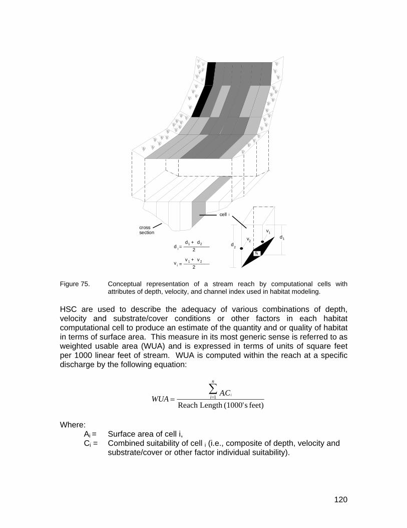
120
Figure 75. Conceptual representation of a stream reach by computational cells with
attributes of depth, velocity, and channel index used in habitat modeling. HSC are used to describe the adequacy of various combinations of depth, velocity and substrate/cover conditions or other factors in each habitat computational cell to produce an estimate of the quantity and or quality of habitat in terms of surface area. This measure in its most generic sense is referred to as weighted usable area (WUA) and is expressed in terms of units of square feet per 1000 linear feet of stream. WUA is computed within the reach at a specific discharge by the following equation:
Where: Ai = Surface area of cell i, Ci = Combined suitability of cell i (i.e., composite of depth, velocity and
substrate/cover or other factor individual suitability).
feet) s(1000' LengthReach1∑==
n
iCA
WUAii
dv 1
2
2d
v1
si
d
v
i
i
=
=
2d21d +__________
2v 21v +__________
cell
crosssection
i

121
The combined or composite suitability of the cell is derived from the aggregation of the individual suitability for depth, velocity, substrate/cover or other factors based on the simulated depth, velocity and substrate/cover attributes within a habitat computational cell. The individual suitabilities for depth, velocity and substrate/cover are obtained from the corresponding species and life stage HSC. The composite suitability can be computed by a number of methods. The most common are the multiplicative, geometric mean, or limiting value approaches. However, as will be discussed below, alternative methods can be used to meet specific modeling objectives. NRC (2004) opined that the modeling approach in the Draft Phase II report for coho was “flawed” given their view that habitat requirements for Chinook were used for coho (page 299) and given life history differences between these two species. We disagree with this contention in part since coho depth and velocity HSC were utilized in the assessments; although we did rely on Chinook escape cover relationships for coho given that these data did not exist. We maintain that coho reliance on cover is well documented in the literature (e.g., Giannico 2000, Hassler 1987, Heifetz et al., 1986) and recent work by Stutzer et al., (2006) in the Klamath River found that coho smolts were most often associated with dense aggregates of vegetation near shore, primarily willows, when not associated with velocity shear zones. This was clearly reflected in the escape cover relationships for Chinook used in the draft report. However, we believe that this issue has been addressed for coho fry with the current analyses that rely on site-specific data from the Klamath River to develop fry HSC, including escape cover relationships. Although we still rely on literature based HSC for coho juvenile and steelhead fry and rely on the corresponding Chinook juvenile or fry escape cover relationships, we believe these relationship adequately reflect escape cover associations for the purposes of modeling given known published literature on the importance of cover for steelhead fry and coho juveniles and from field observations by tribal, state and federal fisheries biologists with extensive experience on the Klamath River. Two-dimensional Based Habitat Modeling The two-dimensional based physical habitat modeling parallels the application of habitat modeling used in PHABSIM. However, due to the spatial nature of the three-dimensional habitat computational mesh a more ‘refined’ habitat analysis is possible compared to typical cross section based approaches employed in most PHABSIM studies as described below. Habitat Computational Mesh Generation As noted previously, the computational meshes used in the hydraulic simulations at all sites contained nodes every 1.6 meters (5.25 feet) across the river and 1.7 meters (5.58 feet) in the longitudinal direction (i.e., up and down the river). The hydraulic solutions at this mesh density were subsequently used to interpolate

122
the hydraulic attributes on 0.61 meter (~ 2.0 feet) meshes for use in habitat modeling as follows. A two-foot curvilinear orthogonal mesh was generated at each of the study sites using a smooth (gradually varying radius) stream centerline overlaid on the DTM of the study site. The spatially explicit substrate and vegetation mapping results, as well as the overlay of the meso-habitat mapping results for each study site was then overlaid on the revised computational mesh and utilized to assign substrate, vegetation and habitat type codes to every node in the refined mesh using the spatial join feature in GIS. GIS was used to construct Triangular Irregular Networks (TINs) from the original depth and velocity solution files at each study site for each simulated flow The TINs were then utilized to interpolate the corresponding depth and velocity at each node within the refined mesh using GIS functions. The interpolated depth and velocity data were compared to the original depth and velocity distributions at all flow rates and these comparisons are provided in Appendix H. Finally, the simulated depths at each modeled flow rate at each site were examined in GIS to identify modeling/interpolation artifacts such as isolated pockets of water in topography depressions and delineated with a polygon. These polygons were then overlaid on the revised computational meshes and used to assign a binary value at each node indicating whether the node should or should not be included when computing physical habitat. Table 21 shows the resulting number of mesh points at each study site used in the habitat simulations Table 21. Number of columns, rows and mesh points used in the curvilinear orthogonal
mesh for habitat simulations at each study site based on interpolation of the hydraulic computational meshes at ~1.6 meters to ~ 0.61 meters spatial resolution.
Study Site Columns Rows Nodes
RRanch 351 1542 541242Trees of Heaven 306 2291 701046Brown Bear 242 1279 309518Seiad 486 3103 1508058Rogers 324 2014 652536Orleans 324 1987 643788Saints Bar 354 1499 530732
Figure 76 shows an example of the verification results at the RRanch study site.

123
Figure 76. Verification of depth and velocity interpolation results at the RRanch study site at
a flow rate of 503 cfs. Top left is velocity for the 2-foot mesh; top right is the velocity from the hydrodynamic model. Bottom left is depth for the 2-foot mesh; bottom right is the depth from the hydrodynamic model.
At a given flow rate, for each node (cell) within the habitat modeling mesh, the integrated data sets included the x and y location, bed elevation, area, simulated depth and mean column velocity, substrate and/or vegetation code, habitat type, habitat exclude flag, and node mesohabitat weighting factor associated with the mesohabitat type (see River Reach Level Habitat Results below). Development of Conceptual Physical Habitat Models Conceptual physical habitat models for each species and life stage were developed through an iterative process that involved the evaluation of different forms of the habitat equations and specific modeling parameters. The iterative process was applied at the RRanch study site by a comparison of the habitat model outputs against the spatial distribution of observed target species and life stages at a single flow rate. Once the computational form of the model and associated parameters were selected, the modeling approach was ‘validated’ against data at the same site at a different flow rate and other study sites where observation data was available for specific species and life stages. Not all study sites or flow rates had fish observation for all species and life stages. Simulation results are only presented for the final model used in the instream flow assessments.

124
USU developed a computer model specifically to implement all the conceptual habitat models evaluated in the study. A test habitat computational grid was constructed with depth, velocity, substrate/vegetation, and habitat exclude variations that was used to manually verify all calculations for each conceptual habitat model against computed values using a spreadsheet. Chinook Spawning Habitat Modeling Chinook spawning habitat was computed on a node-by-node basis from the HSC values for depth, velocity, and substrate, which corresponds to the most commonly applied habitat variables in applied instream flow assessments this life stage across a wide array of salmonids species. The composite suitability (CSI) for a given node was computed as the geometric mean of the individual velocity (VelocitySI), depth (DepthSI) and channel index (substrate) suitabilities (SubstrateSI): CSI = (DepthSI * VelocitySI * SubstrateSI)1/3 Steelhead 1+ Habitat Modeling Based on comparisons between observed and predicted habitat utilization using a variety of computational approaches with combinations of depth, velocity, substrate, cover, and distance to escape cover, the best results for steelhead 1+ were obtained using only the geometric mean of the depth and velocity HSC: CSI = = (DepthSI * VelocitySI)1/2 Fry and Juvenile Escape Cover Modeling for Chinook and Coho The final form of the conceptual habitat models for these species and life stages utilized depth and velocity HSC in conjunction with escape cover types and distance from escape cover HSC. In addition, the conceptual habitat models for these species and life stages also incorporated parameters for an escape cover depth threshold and an escape cover velocity threshold. The basic form of the conceptual habitat model has the form:
CSI = (DepthSI * VelocitySI)1/2 * CompositeEscapeCoverSI Where the CompositeEscapeCoverSI is the area weighted average of the composite suitability of all nodes within the specified distance to escape cover relationship (DistECSI), having a specific type of escape cover (EscapeCoverSI) that meets the escape cover depth threshold (ECDepthThresholdSI) and the escape cover velocity threshold (ECVelThresholdSI) as noted below.
CompositeEscapeCoverSI = EscapeCoverSI * DistECSI * ECDepthThresholdSI * ECVelThresholdSI

125
The distance to escape cover was either binary (e.g., Chinook, coho, steelhead fry) or a functional relationship with distance (e.g., Chinook, coho, steelhead juvenile). The escape cover depth threshold (ECDepthThresholdSI) is a binary value and is utilized to ensure that any node within the specified distance to escape cover is at least that depth or more to ensure that the fish has access to the node at that flow rate. The escape cover velocity threshold (ECVelThresholdSI) is a binary value and is utilized to ensure that any node within the specified distance to escape cover has a velocity less than the indicated value at that flow rate to ensure the node does not have a limiting velocity. The depth and velocity threshold values were developed through discussions with the Technical Team. Table 22 provides a summary of the depth and velocity escape cover threshold values used for fry and juvenile modeling. Table 22. Habitat model parameters for escape cover depth and velocity thresholds for
each relevant species and life stage. Escape Cover Thresholds
Species/Life Stage Depth (ft) Velocity (ft/s) Chinook Juvenile 0.60 3.50 Coho Juvenile 0.60 2.50 Steelhead Juvenile 0.60 4.00 Chinook Fry 0.30 2.00 Coho Fry 0.30 1.50 Steelhead Fry 0.30 1.50
Habitat Modeling Field Validation Habitat simulations for each species and life stage were initially conducted at each study site without any reach level weightings (i.e., node weight values = 1.0). These site-specific habitat simulations were utilized at each intensive study site to empirically validate the habitat modeling. For any species and life stages evaluated in the habitat modeling for which actual fish observations were available, a comparison between fish location and habitat modeling results was undertaken. Field data collections undertaken by state, federal, and tribal biologists in support of the Phase II work were provided to USU. These data delineated the spatial location of specific species and life stages and the flow rate at which the data were observed. Several flow rates were typically sampled at each study location. The number of fish observations also varied by date, location, species, and life stage. All available fish observation data were utilized for the comparisons. These data were used to overlay the fish locations on the orthophotos at each study site and were represented as colored circles on the images.

126
The simulated combined suitability at all nodes associated with a particular flow rate was used to generate contours of suitable habitat between 0.00001 and 1.0 to visualize the spatial distribution of predicted habitat at each study site. Setting the lower threshold at 0.00001 eliminated completely non-suitable conditions from the contoured overlays of habitat. In the following figures, nodes with combined suitability less than this lower threshold are therefore ‘transparent’ and the underlying image of the river is visible. It should be noted when examining these results that the computational mesh for each study site does not encompass the extreme upstream or downstream sections of the visible river in each orthophotograph. Some fish observations shown at the extreme upstream and downstream sections in the images are in fact outside the ‘model spatial domain’ and modeling results should not be interpreted as providing no habitat values in these areas. These circumstances are noted where appropriate in the figure legends. Care should also be taken when comparing predicted habitat quality and fish observations. In several instances, observed flow rates associated with fish collections are not identical to the flow rates associated with the habitat simulations used in comparisons. This is noted where appropriate in the figure legends. It should also be understood that the flow depicted in the imagery (flow when aerial photos were taken) is not always near the flow magnitude used in the modeling comparisons. Therefore, modeled stream boundaries (i.e., edge of water) and fish locations may be higher or lower than the water depicted in the images. This is readily apparent in some instances where fish appear to be located on ‘dry ground’. It is also important to realize that fish observations occurred only within small sections of the study sites. Therefore, suitable habitat that contains no fish observations typically occur because no sampling occurred in these areas. Finally, it should be noted that fish observation data shown in the comparisons also contain observation data not utilized in the development of site-specific HSC and therefore we believe they represent validation data of the habitat modeling. Chinook Spawning Figures 77 through 85 show predicted habitat suitability (i.e., combined suitability at each node) versus the spatial location of Chinook spawning redds at different flow rates for various study sites where observation data was available. It is clear from an examination of these results that there is generally excellent agreement between predicted and observed spatial distribution of redds at different flow rates and locations within the main stem Klamath River. Note in Figures 78 and 79 that a few redd locations were found in a ‘patch’ of stream (upper right center) that the model indicates is not suitable (i.e., no color). This area has substrate delineations that are too coarse for Chinook spawning in the model although the depths and velocity were suitable. Field biologists indicate that this area has ‘small patches’ of suitable gravel behind large substrate
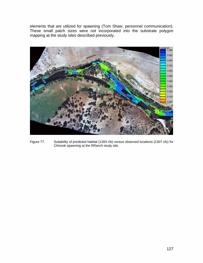
127
elements that are utilized for spawning (Tom Shaw, personnel communication). These small patch sizes were not incorporated into the substrate polygon mapping at the study sites described previously.
Figure 77. Suitability of predicted habitat (1393 cfs) versus observed locations (1307 cfs) for
Chinook spawning at the RRanch study site.

128
Figure 78. Suitability of predicted habitat (1393 cfs) versus observed locations (1377 cfs) for
Chinook spawning at the RRanch study site.
Figure 79. Suitability of predicted habitat (1900 cfs) versus observed locations (1766 cfs) for
Chinook spawning at the RRanch study site.

129
In the previous three images, the highly suitable habitat to the lower right of the island is know to contain spawning redds (USFWS, unpublished field observations) although these redd locations were not surveyed in the collections.
Figure 80. Suitability of predicted habitat (1224 cfs) versus observed locations (1307 cfs) for
Chinook spawning at the Trees of Heaven study site. The slightly lower simulated flow accounts for the apparent lack of predicted habitat at redd locations at the center right channel location.

130
Figure 81. Suitability of predicted habitat (1224 cfs) versus observed locations (1377 cfs) for
Chinook spawning at the Trees of Heaven study site. The slightly lower simulated flow accounts for the apparent lack of predicted habitat at redd locations at the center right channel location.

131
Figure 82. Suitability of predicted habitat (1629 cfs) versus observed locations (1766 cfs) for
Chinook spawning at the Trees of Heaven study site.
Figure 83. Suitability of predicted habitat (1629 cfs) versus observed locations (1483 cfs) for
Chinook spawning at the Brown Bear study site.

132
Figure 84. Suitability of predicted habitat (1469 cfs) versus observed locations (1766 cfs) for
Chinook spawning at the Seiad study site. Fish at upper left in image are outside the boundary of computational mesh.
Figure 85. Suitability of predicted habitat (2083 cfs) versus observed locations (1801 cfs) for
Chinook spawning at the Seiad study site. Fish at upper left and lower right in image are outside the boundary of computational mesh.

133
The simulation results shown above demonstrate that the habitat modeling works extremely well over a wide range of observed discharges and across a variety of study sites with very different habitat availability features. Based on these results we place a high degree of confidence in these modeling results and consider that the Chinook spawning habitat model has been validated. Chinook Fry Figures 86 through 96 show predicted habitat suitability (i.e., combined suitability at each node) versus the spatial location of Chinook fry collected at different flow rates for various study sites where observation data was available.
Figure 86. Suitability of predicted habitat (5548 cfs) versus observed locations (5226 cfs) for
Chinook fry at the RRanch study site.

134
Figure 87. Suitability of predicted habitat (5221 cfs) versus observed locations (5191 cfs) for
Chinook fry at the Trees of Heaven study site.
Figure 88. Suitability of predicted habitat (5858 cfs) versus observed locations (5968 cfs) for
Chinook fry at the Trees of Heaven study site.

135
Figure 89. Suitability of predicted habitat (5489 cfs) versus observed locations (5191 cfs) for
Chinook fry at the Brown Bear study site.
Figure 90. Suitability of predicted habitat (6180 cfs) versus observed locations (5862 cfs) for
Chinook fry at the Brown Bear study site.

136
Figure 91. Suitability of predicted habitat (8380 cfs) versus observed locations (8475 cfs) for
Chinook fry at the Seiad study site. Note that the patch of suitable habitat adjacent to the fish at this simulated flow expands in area at next higher simulated flow (9340 cfs) and overlaps these fish locations.
Figure 92. Suitability of predicted habitat (8380 cfs) versus observed locations (8475 cfs) for
Chinook fry at the Seiad study site.

137
Figure 93. Suitability of predicted habitat (3198 cfs) versus observed locations (3355 cfs) for
Chinook fry at the Orleans study site. The simulation results shown above for Chinook fry demonstrate that the habitat modeling works extremely well over a wide range of observed discharges and across a variety of study sites with very different habitat availability features. In particular, the incorporation of escape cover dependencies in the habitat simulations show a pattern of habitat in terms of spatial distribution and relative suitability that closely matches observed behavior and distribution in the river. It should be pointed out, that fish habitat utilization is not expected to always occur in the highest combined suitability habitats for a variety of reasons as discussed at the beginning of the HSC Section of the report (e.g., predation, temperature, food availability, presence of predators, etc). However, it is expected that fish distributions should be spatially distributed in a ‘presence or absence’ manner associated with useable (i.e., combined suitability > 0.0) versus non-usable (i.e., combined suitability = 0.0) habitats. Based on these results we place a high degree of confidence in these modeling results and consider the habitat model for Chinook fry to be validated. Steelhead Fry Figures 94 and 95 show predicted habitat suitability (i.e., combined suitability at each node) versus the spatial location of steelhead fry collected at a flow rate of 1307 and 1342 cfs at the RRanch study. These simulation results were generated using the generalized HSC as discussed above and therefore
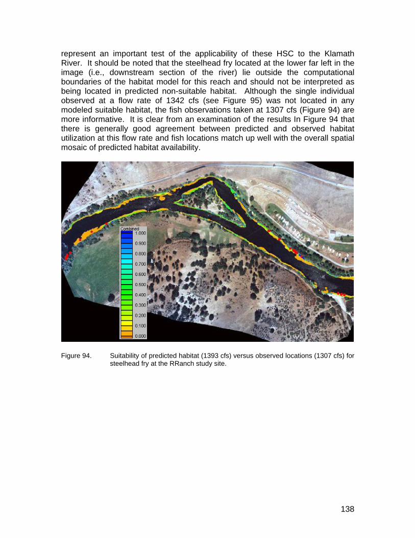
138
represent an important test of the applicability of these HSC to the Klamath River. It should be noted that the steelhead fry located at the lower far left in the image (i.e., downstream section of the river) lie outside the computational boundaries of the habitat model for this reach and should not be interpreted as being located in predicted non-suitable habitat. Although the single individual observed at a flow rate of 1342 cfs (see Figure 95) was not located in any modeled suitable habitat, the fish observations taken at 1307 cfs (Figure 94) are more informative. It is clear from an examination of the results In Figure 94 that there is generally good agreement between predicted and observed habitat utilization at this flow rate and fish locations match up well with the overall spatial mosaic of predicted habitat availability.
Figure 94. Suitability of predicted habitat (1393 cfs) versus observed locations (1307 cfs) for
steelhead fry at the RRanch study site.
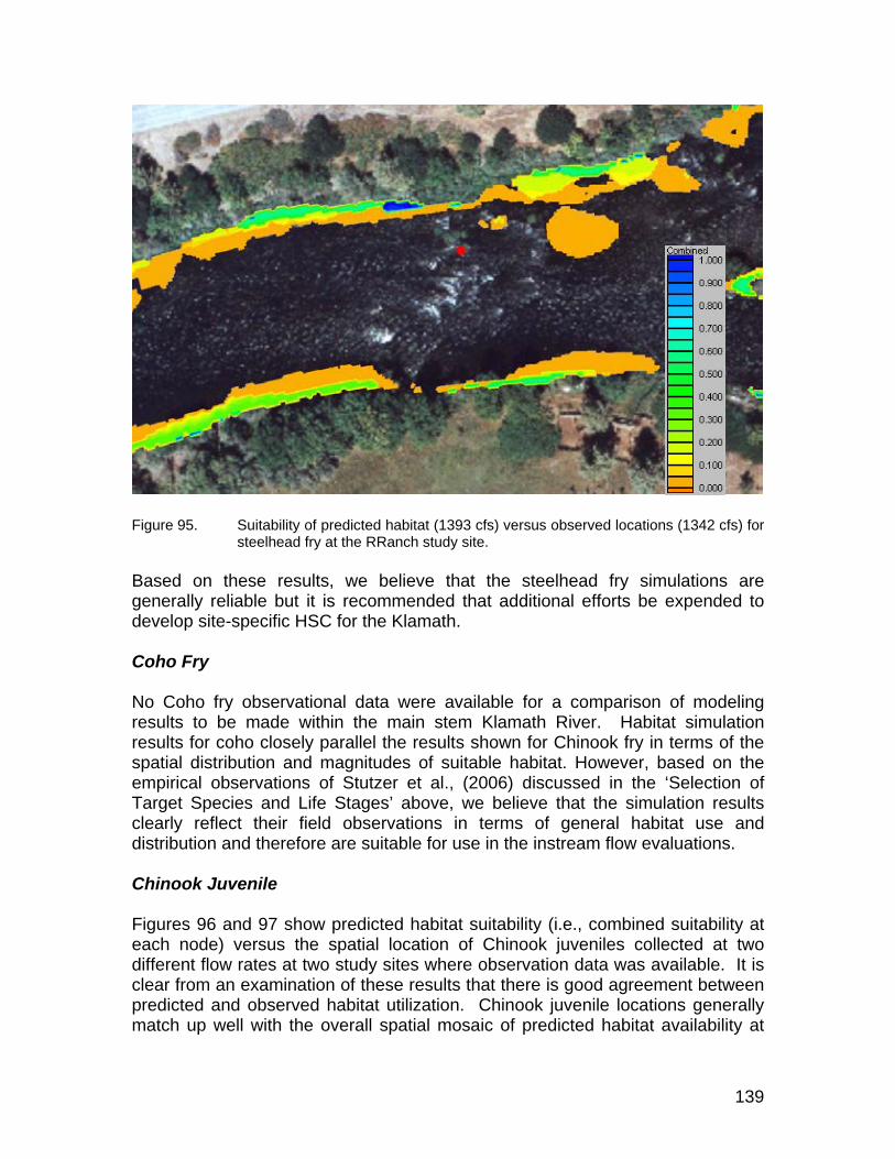
139
Figure 95. Suitability of predicted habitat (1393 cfs) versus observed locations (1342 cfs) for
steelhead fry at the RRanch study site. Based on these results, we believe that the steelhead fry simulations are generally reliable but it is recommended that additional efforts be expended to develop site-specific HSC for the Klamath. Coho Fry No Coho fry observational data were available for a comparison of modeling results to be made within the main stem Klamath River. Habitat simulation results for coho closely parallel the results shown for Chinook fry in terms of the spatial distribution and magnitudes of suitable habitat. However, based on the empirical observations of Stutzer et al., (2006) discussed in the ‘Selection of Target Species and Life Stages’ above, we believe that the simulation results clearly reflect their field observations in terms of general habitat use and distribution and therefore are suitable for use in the instream flow evaluations. Chinook Juvenile Figures 96 and 97 show predicted habitat suitability (i.e., combined suitability at each node) versus the spatial location of Chinook juveniles collected at two different flow rates at two study sites where observation data was available. It is clear from an examination of these results that there is good agreement between predicted and observed habitat utilization. Chinook juvenile locations generally match up well with the overall spatial mosaic of predicted habitat availability at

140
these sites. More extensive observational data at a wider range of flows and at more study site locations would benefit these comparisons. However, for the available data, the modeling results support the efficacy of the habitat modeling for Chinook juveniles in their application for instream assessments within the Klamath River.
Figure 96. Suitability of predicted habitat (1393 cfs) versus observed locations (1342 cfs) for
Chinook juvenile at the RRanch study site.
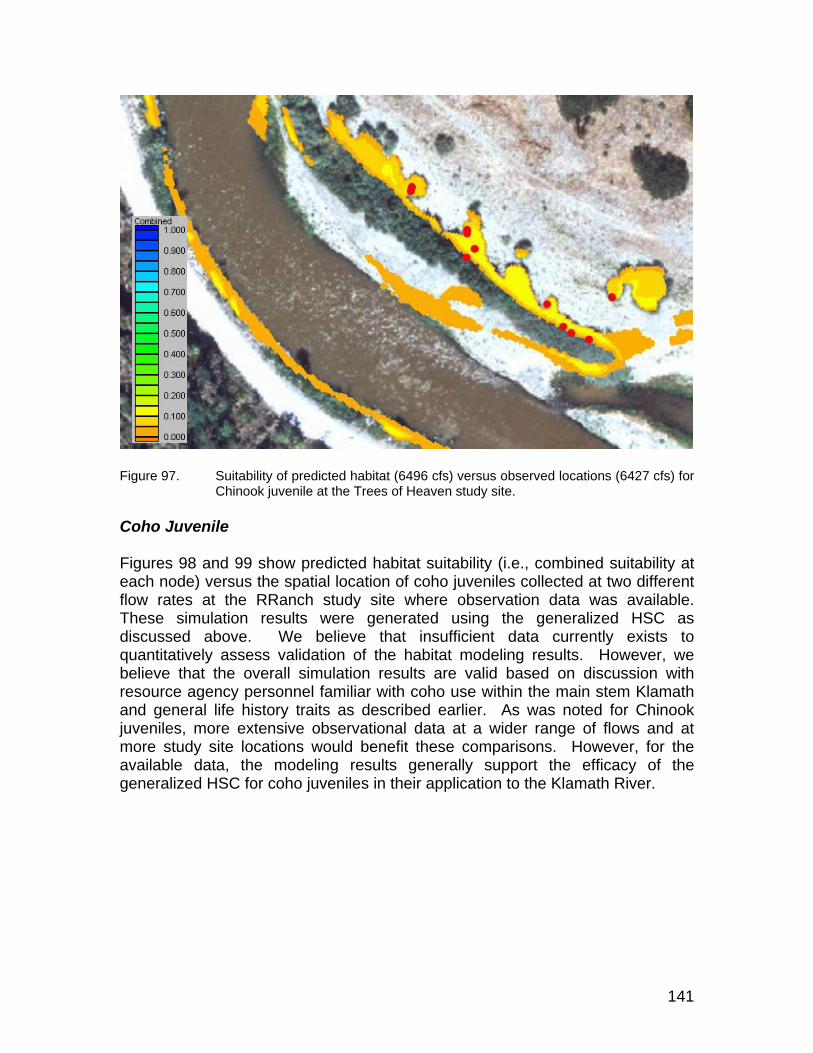
141
Figure 97. Suitability of predicted habitat (6496 cfs) versus observed locations (6427 cfs) for
Chinook juvenile at the Trees of Heaven study site. Coho Juvenile Figures 98 and 99 show predicted habitat suitability (i.e., combined suitability at each node) versus the spatial location of coho juveniles collected at two different flow rates at the RRanch study site where observation data was available. These simulation results were generated using the generalized HSC as discussed above. We believe that insufficient data currently exists to quantitatively assess validation of the habitat modeling results. However, we believe that the overall simulation results are valid based on discussion with resource agency personnel familiar with coho use within the main stem Klamath and general life history traits as described earlier. As was noted for Chinook juveniles, more extensive observational data at a wider range of flows and at more study site locations would benefit these comparisons. However, for the available data, the modeling results generally support the efficacy of the generalized HSC for coho juveniles in their application to the Klamath River.

142
Figure 98. Suitability of predicted habitat (1393 cfs) versus observed locations (1307 cfs) for
coho juvenile at the RRanch study site.
Figure 99. Suitability of predicted habitat (1393 cfs) versus observed locations (1342 cfs) for
coho juvenile at the RRanch study site.

143
Steelhead Juvenile Figures 100 through 106 show predicted habitat suitability (i.e., combined suitability at each node) versus the spatial location of steelhead juveniles collected at different flow rates and various study sites where observation data was available.
Figure 100. Suitability of predicted habitat (1393 cfs) versus observed locations (1307 cfs) for
steelhead juvenile at the RRanch study site.

144
Figure 101. Suitability of predicted habitat (1393 cfs) versus observed locations (1342 cfs) for
steelhead juvenile at the RRanch study site.
Figure 102. Suitability of predicted habitat (5858 cfs) versus observed locations (5968 cfs) for
steelhead juvenile at the Trees of Heaven study site.

145
Figure 103. Suitability of predicted habitat (1469 cfs) versus observed locations (1518 cfs) for
steelhead juvenile at the Seiad study site.
Figure 104. Suitability of predicted habitat (1469 cfs) versus observed locations (1554 cfs) for
steelhead juvenile at the Seiad study site.

146
Figure 105. Suitability of predicted habitat (1469 cfs) versus observed locations (1624 cfs) for
steelhead juvenile at the Seiad study site.

147
Figure 106. Suitability of predicted habitat (2120 cfs) versus observed locations (2225 cfs) for
steelhead juvenile at the Orleans study site. Fish at lower right are outside computational mesh.
It is clear from an examination of these results that there is generally good agreement between predicted and observed habitat utilization over different flow rates and at different stations. We consider that the habitat modeling results for this species and life stage to be suitable for use in the instream flow assessments.
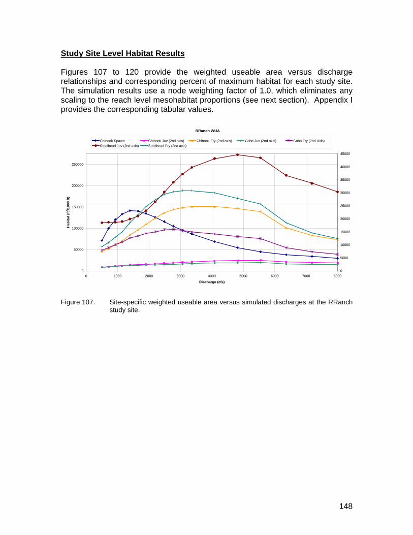
148
Study Site Level Habitat Results Figures 107 to 120 provide the weighted useable area versus discharge relationships and corresponding percent of maximum habitat for each study site. The simulation results use a node weighting factor of 1.0, which eliminates any scaling to the reach level mesohabitat proportions (see next section). Appendix I provides the corresponding tabular values.
Figure 107. Site-specific weighted useable area versus simulated discharges at the RRanch
study site.
RRanch WUA
0
50000
100000
150000
200000
250000
0 1000 2000 3000 4000 5000 6000 7000 8000
Discharge (cfs)
Hab
itat (
ft2 /100
0 ft)
0
5000
10000
15000
20000
25000
30000
35000
40000
45000
Chinook Spawn Chinook Juv (2nd axis) Chinook Fry (2nd axis) Coho Juv (2nd axis) Coho Fry (2nd Axis)Steelhead Juv (2nd axis) Steelhead Fry (2nd axis)

149
Figure 108. Site-specific weighted useable area versus simulated discharges at the Tree of
Heaven study site.
Figure 109. Site-specific weighted useable area versus simulated discharges at the Brown
Bear study site.
Trees of Heaven WUA
0
50000
100000
150000
200000
0 1000 2000 3000 4000 5000 6000 7000 8000 9000
Discharge (cfs)
Hab
itat (
ft2 /100
0 ft)
Chinook Spawn Chinook Juv Chinook Fry Coho Juv Coho Fry Steelhead Juv Steelhead Fry
Brown Bear WUA
0
20000
40000
60000
80000
100000
120000
140000
160000
0 1000 2000 3000 4000 5000 6000 7000 8000 9000
Discharge (cfs)
Hab
itat (
ft2 /100
0 ft)
0
500
1000
1500
2000
2500
3000
Chinook Spawn Chinook Juv (2nd axis) Chinook Fry (2nd axis) Coho Juv (2nd axis) Coho Fry (2nd axis)Steelhead Juv (2nd axis) Steelhead Fry (2nd axis)
150
Figure 110. Site-specific weighted useable area versus simulated discharges at the Seiad
study site.
Figure 111. Site-specific weighted useable area versus simulated discharges at the Rogers
Creek study site.
Seiad WUA
0
100000
200000
300000
400000
500000
0 1000 2000 3000 4000 5000 6000 7000 8000 9000 10000
Discharge (cfs)
Hab
itat (
ft2 /100
0 ft)
0
5000
10000
15000
20000
25000
30000
35000
40000
45000
Chinook Spawn Chinook Juv (2nd axis) Chinook Fry (2nd axis) Coho Juv (2nd axis) Coho Fry (2nd axis)Steelhead Juv (2nd axis) Steelhead Fry (2nd axis)
Rogers WUA
0
20000
40000
60000
80000
100000
120000
140000
160000
180000
0 1000 2000 3000 4000 5000 6000 7000 8000 9000 10000 11000 12000 13000
Discharge (cfs)
Hab
itat (
ft2 /100
0 ft)
0
5000
10000
15000
20000
25000
Chinook Spawn Chinook Juv (2nd axis) Chinook Fry (2nd axis) Coho Juv (2nd axis) Coho Fry (2nd axis)Steelhead Juv (2nd axis) Steelhead Fry (2nd axis)
151
Figure 112. Site-specific weighted useable area versus simulated discharges at the Orleans
study site.
Figure 113. Site-specific weighted useable area versus simulated discharges at the Saints
Rest Bar study site.
Orleans WUA
0
50000
100000
150000
200000
250000
300000
0 1000 2000 3000 4000 5000 6000 7000 8000 9000 10000 11000 12000 13000 14000 15000 16000
Discharge (cfs)
Hab
itat (
ft2 /100
0 ft)
0
500
1000
1500
2000
2500
3000
3500
Chinook Spawn Chinook Juv (2nd axis) Chinook Fry (2nd axis) Coho Juv (2nd axis) Coho Fry (2nd axis)Steelhead Juv (2nd axis) Steelhead Fry (2nd axis)
Saints Rest Bar WUA
0
20000
40000
60000
80000
100000
120000
0 2000 4000 6000 8000 10000 12000 14000 16000 18000
Discharge (cfs)
Hab
itat (
ft2 /100
0 ft)
0
1000
2000
3000
4000
5000
6000
7000
8000
Chinook Spawn Chinook Juv (2nd axis) Chinook Fry (2nd axis) Coho Juv (2nd axis) Coho Fry (2nd axis)Steelhead Juv (2nd axis) Steelhead Fry (2nd axis)
152
Figure 114. Site-specific percent of maximum habitat versus simulated discharges at the
RRanch study site.
Figure 115. Site-specific percent of maximum habitat versus simulated discharges at the
Tree of Heaven study site.
RRanch
0
10
20
30
40
50
60
70
80
90
100
0 1000 2000 3000 4000 5000 6000 7000 8000
Discharge (cfs)
Perc
ent o
f Max
imum
Hab
itat
Chinook Spawn Chinook Juv Chinook Fry Coho Juv Coho Fry Steelhead Juv Steelhead Fry
Trees of Heaven
0
10
20
30
40
50
60
70
80
90
100
0 1000 2000 3000 4000 5000 6000 7000 8000 9000
Discharge (cfs)
Perc
ent o
f Max
imum
Hab
itat
Chinook Spawn Chinook Juv Chinook Fry Coho Juv Coho Fry Steelhead Juv Steelhead Fry

153
Figure 116. Site-specific percent of maximum habitat versus simulated discharges at the
Brown Bear study site.
Figure 117. Site-specific percent of maximum habitat versus simulated discharges at the
Seiad study site.
Brown Bear
0
10
20
30
40
50
60
70
80
90
100
0 1000 2000 3000 4000 5000 6000 7000 8000 9000
Discharge (cfs)
Perc
ent o
f Max
imum
Hab
itat
Chinook Spawn Chinook Juv Chinook Fry Coho Juv Coho Fry Steelhead Juv Steelhead Fry
Seiad
0
10
20
30
40
50
60
70
80
90
100
0 1000 2000 3000 4000 5000 6000 7000 8000 9000 10000
Discharge (cfs)
Perc
ent o
f Max
imum
Hab
itat
Chinook Spawn Chinook Juv Chinook Fry Coho Juv Coho Fry Steelhead Juv Steelhead Fry

154
Figure 118. Site-specific percent of maximum habitat versus simulated discharges at the Rogers Creek study site.
Figure 119. Site-specific percent of maximum habitat versus simulated discharges at the
Orleans study site.
Rogers
0
10
20
30
40
50
60
70
80
90
100
0 1000 2000 3000 4000 5000 6000 7000 8000 9000 10000 11000 12000 13000
Discharge (cfs)
Perc
ent o
f Max
imum
Hab
itat
Chinook Spawn Chinook Juv Chinook Fry Coho Juv Coho Fry Steelhead Juv Steelhead Fry
Orleans
0
10
20
30
40
50
60
70
80
90
100
0 1000 2000 3000 4000 5000 6000 7000 8000 9000 10000 11000 12000 13000 14000 15000 16000
Discharge (cfs)
Perc
ent o
f Max
imum
Hab
itat
Chinook Spawn Chinook Juv Chinook Fry Coho Juv Coho Fry Steelhead Juv Steelhead Fry

155
Figure 120. Site-specific percent of maximum habitat versus simulated discharges at the
Saints Rest Bar study site. The habitat versus discharge relationships depicted above for the various study sites suggest that at most study sites, the habitat availability for life stages of anadromous species are maximized at seasonal flow ranges corresponding to the ‘natural flows’ estimated below Iron Gate Dam. River Reach Level Habitat Results USU Study Site Weightings for Reach Level Habitat Results The USGS/USFWS field based habitat mapping results were overlaid on the orthrophoto of each study site. GIS was then used to assign each node in the computational mesh the appropriate mesohabitat classification. An example of this at the RRanch study site is illustrated in Figure 121.
Saints Rest Bar
0
10
20
30
40
50
60
70
80
90
100
0 2000 4000 6000 8000 10000 12000 14000 16000 18000
Discharge (cfs)
Perc
ent o
f Max
imum
Hab
itat
Chinook Spawn Chinook Juv Chinook Fry Coho Juv Coho Fry Steelhead Juv Steelhead Fry

156
Figure 121. Example of the overlay of field based habitat mapping results on the RRanch
study site used as a basis to assign habitat type attributes to each computational node element.
The mesohabitat mapping results were used to scale the data at each study site to represent the total surface area for each habitat type within their respective river reaches. The surface area of each mesohabitat type that was computed at the reach level was used to assign appropriate weighting factors to each computational node element. Table 23 provides the starting and ending river miles for each of the five river segments and the proportion of available mesohabitats within each segment. Assigning both the habitat type and proportional weight to each computational node element allowed the total habitat versus discharge relationships at the reach level to be computed directly from the habitat modeling results. Study site-specific habitat versus discharge relationships were also computed by assigning the node specific weighting factors a value of 1.0. This essentially computes habitat for the study site without proportioning the habitat availability to the reach level. In both instances, the weighting factor multiplies the area associated with each computational node to scale the results to the appropriate reach level or site-specific level. The site-specific habitat modeling at each USU 2-dimensional study site was ‘scaled’ to the reach level by assigning reach level weightings to each node based on the nodes assigned mesohabitat classification.

157
Table 23. Starting and ending river miles for each river segment and proportion of available mesohabitat types within each segment.
Figures 122 through 128 provide the reach level relationships between habitat and discharge for the four reach level segments used in this analysis. Figures 129 through 135 provide this same information where the habitat has been normalized for each species and life stage to the percent of maximum habitat. Appendix I contains the corresponding tabular data for these results.
SegmentsIron Gate Dam to Shasta River
Shasta River to Scott River
Scott River to Salmon River
Salmon River to Trinity River
Trinity River to Estuary
Starting Mile 0.00 13.45 46.94 125.23 148.10Ending Mile 13.45 46.94 125.23 148.10 194.07Segment Length (mi.) 13.45 33.49 78.29 22.87 45.97Mesohabitat
Main Channel Percent Percent Percent Percent PercentLS 35.03 25.42 13.13 10.64 22.34MS 20.93 19.62 16.32 11.84 12.63SS 3.38 7.38 7.83 6.84 1.33
P 40.66 46.61 60.21 70.18 61.24RUN 0.00 0.97 2.51 0.49 0.96POW 0.00 0.00 0.00 0.00 1.50
UNKNOWN 0.00 0.00 0.00 0.00 0.00Totals 100.00 100.00 100.00 100.00 100.00
MesohabitatSide Channel Percent Percent Percent Percent Percent
LS 22.18 28.37 29.31 31.56 37.96MS 24.60 23.70 14.13 21.11 16.55SS 0.00 4.52 10.58 7.35 0.00
P 45.46 43.41 35.45 39.98 45.49RUN 7.76 0.00 1.71 0.00 0.00
UNKNOWN 0.00 0.00 8.82 0.00 0.00Totals 100.00 100.00 100.00 100.00 100.00
MesohabitatSplit Channel Percent Percent Percent Percent Percent
LS 58.59 20.97 50.55 0.00 39.09MS 29.37 26.12 32.66 0.00 37.34SS 0.00 17.73 8.80 0.00 0.00
P 12.03 35.17 7.99 0.00 23.56RUN 0.00 0.00 0.00 0.00 0.00
UNKNOWN 0.00 0.00 0.00 0.00 0.00Totals 100.00 100.00 100.00 0.00 100.00
158
Figure 122. Reach scaled weighted useable area versus simulated discharges at the RRanch
study site.
Figure 123. Reach scaled weighted useable area versus simulated discharges at the Tree of
Heaven study site.
RRanch WUA
0
10000
20000
30000
40000
50000
60000
0 1000 2000 3000 4000 5000 6000 7000 8000
Discharge (cfs)
Hab
itat (
ft2 /100
0 ft)
0
1000
2000
3000
4000
5000
6000
7000
8000
Chinook Spawn Chinook Juv (2nd axis) Chinook Fry (2nd axis) Coho Juv (2nd axis) Coho Fry (2nd Axis)Steelhead Juv (2nd axis) Steelhead Fry (2nd axis)
Trees of Heaven WUA
0
5000
10000
15000
20000
25000
30000
0 1000 2000 3000 4000 5000 6000 7000 8000 9000
Discharge (cfs)
Hab
itat (
ft2 /100
0 ft)
Chinook Spawn Chinook Juv Chinook Fry Coho Juv Coho Fry Steelhead Juv Steelhead Fry
159
Figure 124. Reach scaled weighted useable area versus simulated discharges at the Brown
Bear study site.
Figure 125. Reach scaled weighted useable area versus simulated discharges at the Seiad
study site.
Brown Bear WUA
0
10000
20000
30000
40000
50000
60000
0 1000 2000 3000 4000 5000 6000 7000 8000 9000
Discharge (cfs)
Hab
itat (
ft2 /100
0 ft)
0
500
1000
1500
2000
2500
3000
Chinook Spawn Chinook Juv (2nd axis) Chinook Fry (2nd axis) Coho Juv (2nd axis) Coho Fry (2nd axis)Steelhead Juv (2nd axis) Steelhead Fry (2nd axis)
Seiad WUA
0
10000
20000
30000
40000
50000
60000
0 1000 2000 3000 4000 5000 6000 7000 8000 9000 10000
Discharge (cfs)
Hab
itat (
ft2 /100
0 ft)
0
500
1000
1500
2000
2500
3000
3500
4000
4500
5000
Chinook Spawn Chinook Juv (2nd axis) Chinook Fry (2nd axis) Coho Juv (2nd axis) Coho Fry (2nd axis)Steelhead Juv (2nd axis) Steelhead Fry (2nd axis)

160
Figure 126. Reach scaled weighted useable area versus simulated discharges at the Rogers Creek study site.
Figure 127. Reach scaled weighted useable area versus simulated discharges at the Orleans
study site.
Rogers WUA
0
5000
10000
15000
20000
25000
0 1000 2000 3000 4000 5000 6000 7000 8000 9000 10000 11000 12000 13000
Discharge (cfs)
Hab
itat (
ft2 /100
0 ft)
0
500
1000
1500
2000
2500
3000
Chinook Spawn Chinook Juv (2nd axis) Chinook Fry (2nd axis) Coho Juv (2nd axis) Coho Fry (2nd axis)Steelhead Juv (2nd axis) Steelhead Fry (2nd axis)
Orleans WUA
0
5000
10000
15000
20000
25000
30000
35000
40000
45000
0 1000 2000 3000 4000 5000 6000 7000 8000 9000 10000 11000 12000 13000 14000 15000 16000
Discharge (cfs)
Hab
itat (
ft2 /100
0 ft)
0
50
100
150
200
250
300
350
400
450
Chinook Spawn Chinook Juv (2nd axis) Chinook Fry (2nd axis) Coho Juv (2nd axis) Coho Fry (2nd axis)Steelhead Juv (2nd axis) Steelhead Fry (2nd axis)

161
Figure 128. Reach scaled weighted useable area versus simulated discharges at the Saints
Rest Bar study site.
Figure 129. Reach scaled percent of maximum habitat versus simulated discharges at the
RRanch study site.
Saints Rest Bar WUA
0
5000
10000
15000
20000
25000
30000
0 2000 4000 6000 8000 10000 12000 14000 16000 18000
Discharge (cfs)
Hab
itat (
ft2 /100
0 ft)
0
200
400
600
800
1000
1200
1400
1600
1800
Chinook Spawn Chinook Juv (2nd axis) Chinook Fry (2nd axis) Coho Juv (2nd axis) Coho Fry (2nd axis)Steelhead Juv (2nd axis) Steelhead Fry (2nd axis)
RRanch
0
10
20
30
40
50
60
70
80
90
100
0 1000 2000 3000 4000 5000 6000 7000 8000
Discharge (cfs)
Perc
ent o
f Max
imum
Hab
itat
Chinook Spawn Chinook Juv Chinook Fry Coho Juv Coho Fry Steelhead Juv Steelhead Fry
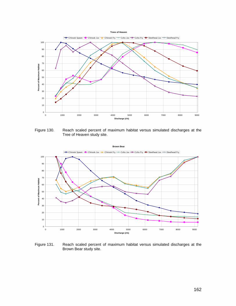
162
Figure 130. Reach scaled percent of maximum habitat versus simulated discharges at the
Tree of Heaven study site.
Figure 131. Reach scaled percent of maximum habitat versus simulated discharges at the
Brown Bear study site.
Trees of Heaven
0
10
20
30
40
50
60
70
80
90
100
0 1000 2000 3000 4000 5000 6000 7000 8000 9000
Discharge (cfs)
Perc
ent o
f Max
imum
Hab
itat
Chinook Spawn Chinook Juv Chinook Fry Coho Juv Coho Fry Steelhead Juv Steelhead Fry
Brown Bear
0
10
20
30
40
50
60
70
80
90
100
0 1000 2000 3000 4000 5000 6000 7000 8000 9000
Discharge (cfs)
Perc
ent o
f Max
imum
Hab
itat
Chinook Spawn Chinook Juv Chinook Fry Coho Juv Coho Fry Steelhead Juv Steelhead Fry
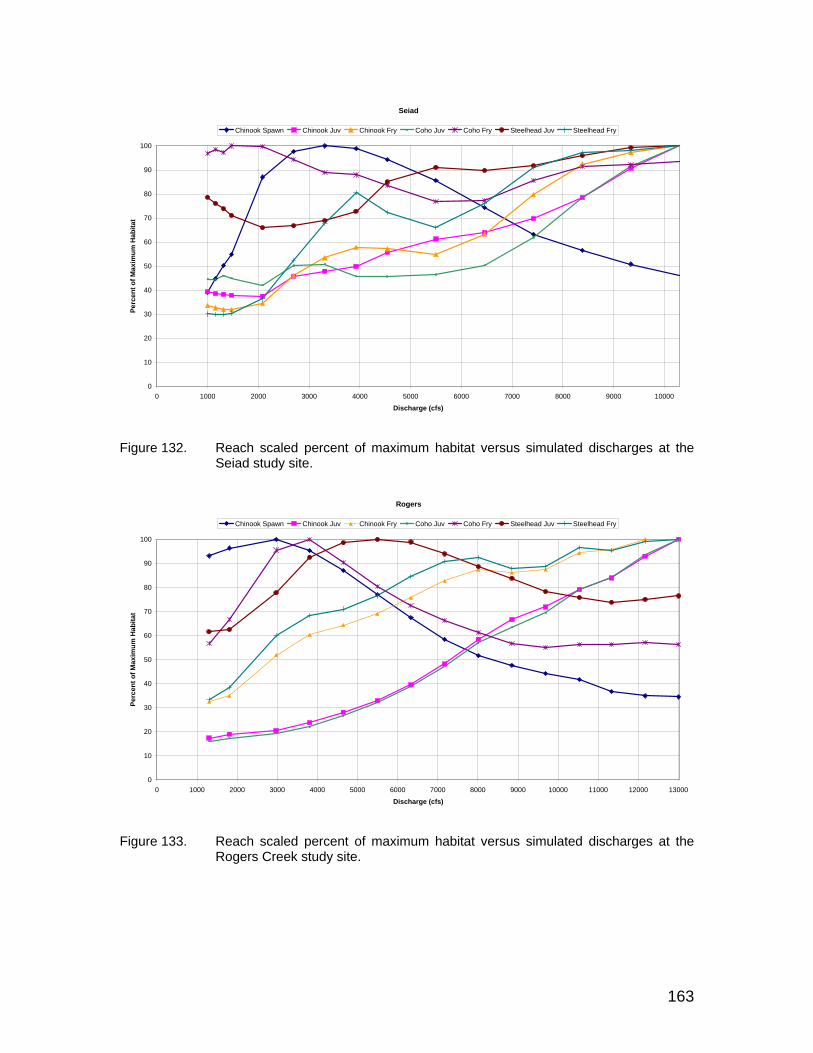
163
Figure 132. Reach scaled percent of maximum habitat versus simulated discharges at the
Seiad study site.
Figure 133. Reach scaled percent of maximum habitat versus simulated discharges at the
Rogers Creek study site.
Seiad
0
10
20
30
40
50
60
70
80
90
100
0 1000 2000 3000 4000 5000 6000 7000 8000 9000 10000
Discharge (cfs)
Perc
ent o
f Max
imum
Hab
itat
Chinook Spawn Chinook Juv Chinook Fry Coho Juv Coho Fry Steelhead Juv Steelhead Fry
Rogers
0
10
20
30
40
50
60
70
80
90
100
0 1000 2000 3000 4000 5000 6000 7000 8000 9000 10000 11000 12000 13000
Discharge (cfs)
Perc
ent o
f Max
imum
Hab
itat
Chinook Spawn Chinook Juv Chinook Fry Coho Juv Coho Fry Steelhead Juv Steelhead Fry

164
Figure 134. Reach scaled percent of maximum habitat versus simulated discharges at the
Orleans study site.
Figure 135. Reach scaled percent of maximum habitat versus simulated discharges at the
Saints Rest Bar study site.
Orleans
0
10
20
30
40
50
60
70
80
90
100
0 1000 2000 3000 4000 5000 6000 7000 8000 9000 10000 11000 12000 13000 14000 15000 16000
Discharge (cfs)
Perc
ent o
f Max
imum
Hab
itat
Chinook Spawn Chinook Juv Chinook Fry Coho Juv Coho Fry Steelhead Juv Steelhead Fry
Saints Rest Bar
0
10
20
30
40
50
60
70
80
90
100
0 2000 4000 6000 8000 10000 12000 14000 16000 18000
Discharge (cfs)
Perc
ent o
f Max
imum
Hab
itat
Chinook Spawn Chinook Juv Chinook Fry Coho Juv Coho Fry Steelhead Juv Steelhead Fry

165
Habitat Time Series Modeling An introduction to physical habitat time series modeling and its application within IFIM type assessment frameworks from a U.S. perspective can be found in Stalnaker et al., (1995). The IFIM literature in its various permutations used in the U.S. and at the international level typically supports the calculation of physical habitat time series as part of project assessments (Harby et al., 2004). Harby et al., (2004) provides an excellent review of the state-of-the-art in instream flow assessment methodologies developed in response to the European Union Water Framework Directives legislation that precipitated these efforts in the form of the COST 626 project14. We calculated the physical habitat time series based on several input flow scenarios. In general, we used the mean monthly flows at our study site locations based on SIAM results for the BOR natural flow and level-pool consumptive use flows using the SIAM no-project alternative and existing conditions for the SIAM with-project simulations as described previously. We also utilized 100 of the stochastic flow series generated from the PARMA modeling to compute physical habitat time series at the RRanch Study Site for all modeled anadromous species and life stages. These simulations were used to examine the expected variance around the habitat time series predictions. The stochastic flow series results at Keno were all adjusted by the same estimated historical accretions to derive flows at Iron Gate (i.e., RRanch Study Site). Mean monthly flows at each study site based on the level-pool unimpaired, natural flow study, existing conditions, and stochastic natural flows were used to compute the corresponding habitat time series based on the species and life stage periodicity for the river (see Table 15). These data were then used to construct monthly habitat duration curves for each species and life stage occupying the river for that particular month. Tabular and graphical results for each month at all study sites that compare the existing hydrology to the estimated unimpaired and natural flows are provided in Appendix J. It should be noted that these simulations do not account for water temperature as a factor, since they are based solely on physical habitat (i.e., depth, velocity, substrate/cover). Water quality and temperature considerations are discussed below. The corresponding ensemble ranges in simulated monthly physical habitat over difference exceedence ranges at the RRanch Study Site are also provided in Appendix J. Figures 136 to 138 provide comparative results for three different species and life stages for three different months at the RRanch study site that illustrates the differential response to simulated habitat for the Natural Flow, level-pool unimpaired, and existing flows. These results are illustrative of the type and 14 The complete report series covering a wide array of instream flow related technical issues can be located at: http://dats.boku.ac.at/

166
magnitude of habitat differences for the various study reaches, species/life stages, and flow regimes contained in Appendix J.
Figure 136. Habitat durations for Chinook spawning at the RRanch study site in October
based on the estimated Natural Flow study, Level-pool unimpaired flows, and existing impaired flows.
Figure 137. Habitat durations for steelhead 1+ (juveniles) at the RRanch study site in July
based on the estimated Natural Flow study, Level-pool unimpaired flows, and existing impaired flows.

167
Figure 138. Habitat durations for coho fry at the RRanch study site in April based on the
estimated Natural Flow study, Level-pool unimpaired flows, and existing impaired flows.
The habitat time series results clearly reflect the differential changes in habitat availability on a seasonal basis, reflective of the seasonal changes in the Klamath River hydrograph associated with existing conditions. The stochastic based ensemble habitat duration results for Chinook juveniles in August are illustrated in Figure 139 and include the 5 and 95 percentiles. We believe these results provide insight to the inherent variability associated with the dynamic template of flow dependent physical habitat in the river, are reflective of the range in this variability for given months and exceedence ranges, and that these results are somewhat insensitive to the input flow series used to develop the PARA model as long as the BOR study captured the basic seasonality of the flow regime at the monthly time step. Our comparisons to the early Keno gage records reported above tend to confirm this.
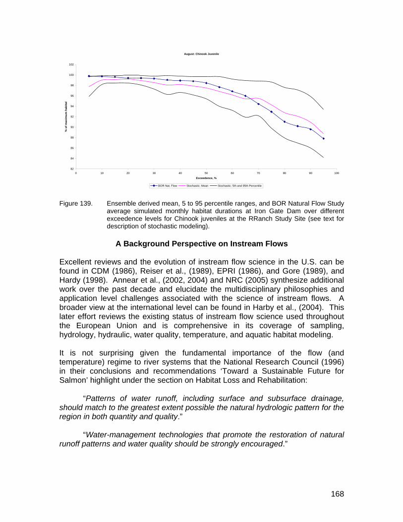
168
Figure 139. Ensemble derived mean, 5 to 95 percentile ranges, and BOR Natural Flow Study
average simulated monthly habitat durations at Iron Gate Dam over different exceedence levels for Chinook juveniles at the RRanch Study Site (see text for description of stochastic modeling).
A Background Perspective on Instream Flows
Excellent reviews and the evolution of instream flow science in the U.S. can be found in CDM (1986), Reiser et al., (1989), EPRI (1986), and Gore (1989), and Hardy (1998). Annear et al., (2002, 2004) and NRC (2005) synthesize additional work over the past decade and elucidate the multidisciplinary philosophies and application level challenges associated with the science of instream flows. A broader view at the international level can be found in Harby et al., (2004). This later effort reviews the existing status of instream flow science used throughout the European Union and is comprehensive in its coverage of sampling, hydrology, hydraulic, water quality, temperature, and aquatic habitat modeling. It is not surprising given the fundamental importance of the flow (and temperature) regime to river systems that the National Research Council (1996) in their conclusions and recommendations ‘Toward a Sustainable Future for Salmon’ highlight under the section on Habitat Loss and Rehabilitation: “Patterns of water runoff, including surface and subsurface drainage, should match to the greatest extent possible the natural hydrologic pattern for the region in both quantity and quality.”
“Water-management technologies that promote the restoration of natural runoff patterns and water quality should be strongly encouraged.”
August: Chinook Juvenile
82
84
86
88
90
92
94
96
98
100
102
0 10 20 30 40 50 60 70 80 90 100
Exceedence, %
% o
f max
imum
hab
itat
BOR Nat. Flow Stochastic: Mean Stochastic: 5th and 95th Percentile

169
This view of the flow regime was reinforced by the Instream Flow Council (2002) work on Instream Flows for Riverine Resource Stewardship and by the NRC (2005) work on The Science of Instream Flows: A Review of the Texas Instream Flow Program. Utilizing the characteristics of the natural flow regime as a ‘template’ is widely accepted and applied at the international level as illustrated by work under the EU Water Framework Directive (Directive 2000/60/EC) by Hardy et al., (2006), Acreman et al., (2006) under EU Water Framework Directive (Directive 2005/48/EC), Dunbar et al., (1998), and Tharme & King (1998) in South Africa under river ecosystem protection legislative mandates. We point out that none of these programs are focused on endangered and threatened species but overall protection of river ecosystems. Adoption of the natural flow paradigm underpins most developed countries river protection, restoration planning, and implementation on an annual and strategic basis (e.g., Harby et al., 2004 and proceedings of the 1st through 5th Ecohydraulics Symposium15, among others). We have broadly adopted the natural flow paradigm in framing our recommendations and integrate concepts from many sources such as the river continuum (Ward and Stanford 1982a), intermediate disturbance hypotheses (Ward and Stanford 1982b), theoretical and realized niche concepts (e.g., Huff et al., 2005), and a large body of material on fish thermal preference, tolerance, and growth. For convenience, we defer introduction of this material where used in support of the recommendation process. NRC (2005) recommended that instream flows consider at least four hydrologic regimes: over bank, high pulse, base, and subsistence flows and are conceptually illustrated in Figure 140.
Figure 140. Illustration of over bank, high pulse, base, and subsistence components of an
annual flow regime.
15 http://www.iahr.net/site/index.html
USGS 11509500 KLAMATH RIVER AT KENO, OR
0
2000
4000
6000
8000
10000
Jan-90 Jan-91 Jan-92 Jan-93 Jan-94
Date
Flow
, cfs
High Flow Pulses
Base FlowSubsistence
Flow
Overbank Flow

170
These components were broadly defined by NRC (2005) as:
• Over Bank An infrequent high flow event that overtops the riverbanks. • High Pulse A short duration high flow within the stream channel during
or immediately after storm events. • Base Average flows in the absence of significant precipitation or
runoff event. • Subsistence Minimum stream flow needed to maintain tolerable water
quality conditions and provide minimal aquatic habitat. Partitioning the flow regime in this manner broadly follows from the functional role each performs in river ecosystems. For example, flow regimes targeting Over Bank Flows (i.e., channel and riparian maintenance) focus on the process driven linkages between flow, sediment transport, and riparian vegetation community phenologies while a base flow regime might focus more on the physical habitat, food and temperature regimes for rearing fish species. A review of FERC license filings shows a considerable variation in the description of the flow regime component being considered and the methodological approaches used to make instream flow recommendations. In many cases, these variations are attributed to site and project specific differences, data availability, and stakeholder driven processes, etc., but are reflective of the variation at the national level, regardless of the legal, institutional, or policy forum. What is in common, however, is the conceptual approach to instream flow recommendations based on different functions performed by the flow regime and their linkages to responses in aquatic ecosystems. Similar conceptual schemes that partition the flow regime into functional components for making instream flow recommendations are widely applied at the international level (e.g., Hughes 1999, Tharme & King (1998), Postel and Richter 2003). A particularly insightful look at the proliferation of proposed hydrologic indices for characterizing flow regimes for use in instream flow assessments can be found in Olden and Poff (2003) who suggested a range of indices associated with duration, magnitude, timing, frequency, and rate of change. He also notes the difficulty in picking a metric and associated threshold associated with ecological response. Protecting or reestablishing these intrinsic properties of the flow regime (however operationally defined or analyzed) is universally considered essential to maintain or recover the ecological health of stream ecosystem functions (e.g., Hill et al., 1991; Kirby and White 1994; Harper and Ferguson 1995; Petts and Calow 1996; Poff et al., 1997; Richter et al., 2003; Annear et al., 2002, 2004; NRC 2002, 2004, 2005). We fully recognize that some characteristics of the natural flow (and thermal) regime are not attainable given limitations imposed by the existing water resource infrastructure beginning at Iron Gate Dam.

171
Flow and Temperature Based Instream Flow Needs The Klamath River ecosystem is composed of physical space in which the processes controlling energy flux across trophic levels vary in time and from an anadromous fish or macroinvertebrate perspective, constrained at the individual, population, and community levels by availability and timing of physical habitat, food resources, and thermal regime16. We approach the development of a conceptual model for anadromous salmonids instream flows using physical habitat relationships to address space needs, while examining the thermal regimes in light of both anadromous and macroinvertebrate thermal niche requirements. The limits of thermal niche are derived from the fundamentals of pokilotherm physiology using published data on thermal preference and tolerance, acute and chronic exposure levels, temperature and food dependent bioenergetic-based growth rates, and behavioral thermoregulation strategies. The energetic modeling is used to corroborate observed behavioral thermoregulation (e.g., use of thermal refugia) by anadromous species in the main stem Klamath River. We consider that there are two dominant processes within the main stem Klamath River represented by the flow and thermal regime. In terms of seasonal anadromous fish exploitation of the river system based on energy dynamics at the individual, population and community levels, the thermal regime may at times be the controlling factor. The simulated minimum, mean, and maximum daily temperatures for existing conditions and for the without project scenario based on hourly simulations using RMA-2/11 for the 2000 to 2004 period are provided in Figure 141 below Iron Gate Dam.
16 We will defer factors such as predation and disease until later.
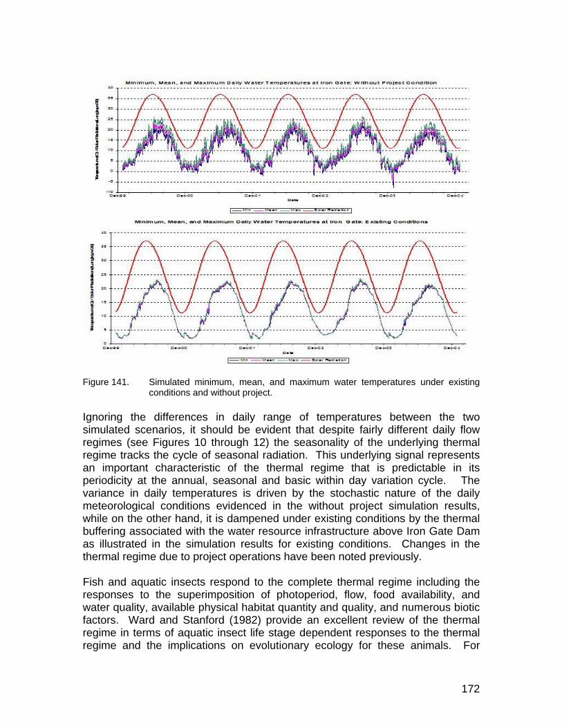
172
Figure 141. Simulated minimum, mean, and maximum water temperatures under existing
conditions and without project. Ignoring the differences in daily range of temperatures between the two simulated scenarios, it should be evident that despite fairly different daily flow regimes (see Figures 10 through 12) the seasonality of the underlying thermal regime tracks the cycle of seasonal radiation. This underlying signal represents an important characteristic of the thermal regime that is predictable in its periodicity at the annual, seasonal and basic within day variation cycle. The variance in daily temperatures is driven by the stochastic nature of the daily meteorological conditions evidenced in the without project simulation results, while on the other hand, it is dampened under existing conditions by the thermal buffering associated with the water resource infrastructure above Iron Gate Dam as illustrated in the simulation results for existing conditions. Changes in the thermal regime due to project operations have been noted previously. Fish and aquatic insects respond to the complete thermal regime including the responses to the superimposition of photoperiod, flow, food availability, and water quality, available physical habitat quantity and quality, and numerous biotic factors. Ward and Stanford (1982) provide an excellent review of the thermal regime in terms of aquatic insect life stage dependent responses to the thermal regime and the implications on evolutionary ecology for these animals. For

173
example, ecological cueing to this predictable periodicity in the thermal regime from seasonal to diel fluctuations has been postulated as a mechanism controlling temporal segregation in macroinvertebrate communities (Ward and Stanford 1982). Disruption to this synchronization or alteration to the variation in amplitude of the thermal range can result in individual, population, and community level responses over both short and evolutionary time scales (Ward and Stanford 1982). It has been argued that the predictable periodicity in seasonal (and even diel) temperatures with expected ranges in variation may be required for evolutionary plasticity in the gene pool. Disruption in the synchronicity of the thermal regime between the main stem and tributary systems for example, has been noted in the Klamath River, where exiting smolts from tributaries containing acceptable thermal conditions encounter adverse thermal regimes in the main stem (Tom Shaw, unpublished field data). Adult spawning strays are an example of a species strategy that encompasses spatial plasticity necessary to accommodate catastrophic landscape level disruptions (e.g., post Mt. Saint Helen stream systems) or longer-term shifts associated with climatic regimes. Components of the Flow Regime Used to Guide the Recommendations We have adapted the recommendations provided in NRC (2005) to target the following components of the flow regime when considering instream flow recommendations:
• Over Bank Flows • High Flow Pulses • Base Flows • Subsistence Flows • Ecological Base Flows17
We use these components as guidelines to formulate our flow recommendations but note that the flow regime is in fact a continuous ‘process’ and that these divisions are somewhat artificial. The quantification of target instream flow recommendations for each component of the flow regime is approached differently. This arises necessarily from the different types and scales of the processes represented by each component, the different temporal scales at which they affect ecosystem processes, and constraints imposed by our ability to measure, model, and predict these processes with some greater or lesser degree of uncertainty. Over Bank and High Flow Pulse recommendations are derived primarily from work conducted on channel geomorphology, sediment transport, and riparian systems. We develop our instream flow recommendations for the remaining components of the flow regime from an integration of hydrology, hydraulics,
17 Ecological Base Flows were not explicitly identified by NRC (2005), see text for definition.
174
water quality, temperature, growth, physical habitat, anadromous species temperature tolerance and preference, and ecological risk associated with flow and temperature regimes on a monthly basis and water year type. Additional factors such as hatchery releases, food production, behavioral thermoregulation, etc., are also incorporated and are often factored across spatial and temporal scales of the flow regime components as would be expected. We have also incorporated material on the emerging issues related to fish disease and disease organism life history when considering our recommendations.
Flow Recommendation Methodology The flow recommendations developed for each component of the flow regime are provided below. The methodology for each component is described and the supporting rationale based on theoretical and empirical data are provided. Over Bank Flows Over Bank flows are infrequent, high flow events that overtop the riverbanks and contribute to floodplain development and maintenance and provide lateral connectivity to off-channel habitats (NRC 2005, Annear et al., 2002, 2004). We equate Over Bank flows with channel and riparian maintenance flows (see Schmidt and Potyondy 2004). Schmidt and Potyondy (2004) provide an excellent review on channel maintenance procedures and provide a variety of techniques applicable to gravel-bed rivers. They suggest that in the absence of extensive site-specific detailed quantitative data that a good indirect approach to channel riparian maintenance flows using 80 percent of the 1.5-year discharge. This would equate to approximately 5800 cfs under existing conditions. By comparison, PacifiCorp (2006) conducted geomorphic analyses including initiation of bed load movement and return periods for existing conditions. These analyses suggest that below Iron Gate Dam, the average return period for flows at the threshold for bed mobility was ~ 13,00018 cfs for existing conditions. The higher flow estimate is in part attributable to the coursing of the bed material immediately below Iron Gate Dam due to upstream trapping of fine sediments. Based on these results, we believe that existing operations of upstream reservoirs, including limited storage capacities are currently maintaining adequate Over Bank flows and that unless substantive additional upstream storage were developed, no remedial prescription for Over Bank Flows are required at this time. High Flow Pulses High Flow Pulses are defined as short-duration, high flow events associated with storm events and provide flushing flows for finer sediments important to maintain quality spawning gravels, lateral connectivity and channel maintenance. Reiser 18 Immediately below Iron Gate the average value was computed as ~ 15,000 cfs while at the RRanch Study Site the average was computed as ~ 12,000 cfs.
175
et al., (2005) provide an excellent review and synthesis of pulse flow effects on benthic macroinvertebrates and fish, the later primarily from a stranding perspective on small fish. Pulse flows have also been recommended in conjunction with storm events in regulated systems as a mechanism to facilitate upstream migration of adult salmon (e.g., Eel River, FERC relicensing conditions). However, limited data collected in the Klamath River on Chinook upstream migration under test flow pulses did not show a response. Migration was delayed associated with water temperatures above ~22 C, and fish movement occurred when temperatures dropped below this value and not associated with the flow pulse (Josh Strange, unpublished data). State and federal resource agencies are currently evaluating use of a water bank for a variety of purposes including pulse flows. We defer setting any specific High Flow Pulse requirements until additional flow pulse tests are evaluated. However, under existing project operations, flow pulses are still evident in the gage data from the main stem Klamath River downstream of Iron Gate Dam associated with tributary inflows and storm events. Base Flows Base Flows are defined as ‘normal’ flow conditions and provide the basic range of flow and temperature/water quality conditions that occur within a given year or between years. Base Flows vary by water year type reflecting the strength of the water year. As noted below, we consider Subsistence Flows and Ecological Base Flows to represent the lower ranges of flows along the exceedence flow continuum (i.e., < 80 percent monthly exceedence levels), while Base Flows are associated with exceedence flow ranges less than 80 percent on a monthly basis. From a fish physical habitat perspective, we approached the flow recommendations for Base Flows from the objective to mimic the pattern and range of flow and habitat conditions estimated under the natural flow regime following the principals of the natural flow paradigm. We recognize that under any ‘natural’ flow regime, ‘optimal’ or maximum habitat conditions do not necessarily occur for a given species or life stage in any or all locations or all time periods. In fact, spatial and temporal variability in habitat availability and quality is necessary to maintain proper ecosystem functions. Integration of the thermal regime is approached primarily from the perspective of thermal limits, behavioral thermoregulation, and bioenergetics to evaluate the growth potential for Chinook and steelhead. Natural Flow Paradigm Derived Flow Estimates The fundamental assumption for estimating this component of the flow regime is that the within year and between year variability of the flows should mimic the basic pattern of the flow regime over all exceedence ranges. We developed an

176
approach that ties the expected flows below Iron Gate Dam to the estimated impaired annual exceedence levels for net Klamath Lake inflows as follows. Annual exceedences were estimated based on Upper Klamath Lake net inflow data adopted from values used in SIAM based on “with project” and “without project” scenarios for the period of record starting with water year 1961 and ending with water year 2000. Annual exceedences were calculated for the mean annual flow (MAF) for each water year19. In order to maintain the linkage between the estimated annual exceedence and corresponding mean monthly flows, all months for that particular annual exceedence level were assigned that year’s exceedence level as illustrated in Table 24. Table 24. Example of assignment of annual exceedence levels to monthly flows.
Water Year Month Flow, cfs
Annual Exceedence
1965 10 1335.94 2.441965 11 1782.42 2.441965 12 6972.57 2.441965 1 6617.74 2.441965 2 5737.62 2.441965 3 3493.01 2.441965 4 2656.33 2.441965 5 2461.74 2.441965 6 1328.02 2.441965 7 772.73 2.441965 8 953.51 2.441965 9 1098.70 2.441974 10 1573.25 4.881974 11 3227.81 4.881974 12 3487.60 4.881974 1 4483.52 4.88
Relationships between monthly flows and annual exceedences for each month were then developed for the Upper Klamath Lake as illustrated in Figure 142.
19 These annual exceedences can be translated to April forecast for implementation purposes.
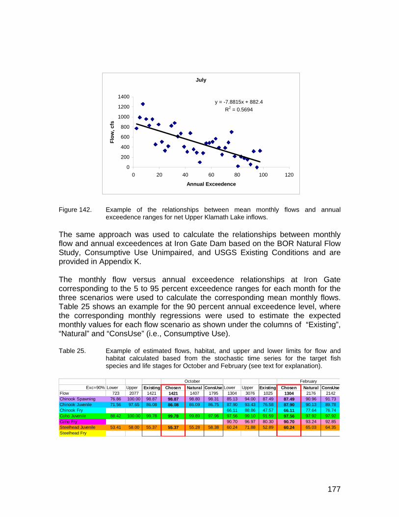
177
Figure 142. Example of the relationships between mean monthly flows and annual
exceedence ranges for net Upper Klamath Lake inflows. The same approach was used to calculate the relationships between monthly flow and annual exceedences at Iron Gate Dam based on the BOR Natural Flow Study, Consumptive Use Unimpaired, and USGS Existing Conditions and are provided in Appendix K. The monthly flow versus annual exceedence relationships at Iron Gate corresponding to the 5 to 95 percent exceedence ranges for each month for the three scenarios were used to calculate the corresponding mean monthly flows. Table 25 shows an example for the 90 percent annual exceedence level, where the corresponding monthly regressions were used to estimate the expected monthly values for each flow scenario as shown under the columns of “Existing”, “Natural” and “ConsUse” (i.e., Consumptive Use). Table 25. Example of estimated flows, habitat, and upper and lower limits for flow and
habitat calculated based from the stochastic time series for the target fish species and life stages for October and February (see text for explanation).
Exc=90% Lower Upper Existing Chosen Natural ConsUse Lower Upper Existing Chosen Natural ConsUseFlow 723 2077 1421 1421 1407 1795 1304 3076 1025 1304 2176 2142Chinook Spawning 76.86 100.00 98.87 98.87 98.80 98.31 85.13 94.00 87.49 87.49 90.96 91.73Chinook Juvenile 71.56 97.65 86.08 86.08 86.09 86.75 87.90 93.43 76.58 87.90 90.13 89.78Chinook Fry 66.11 88.86 47.57 66.11 77.64 76.74Coho Juvenile 88.42 100.00 99.78 99.78 99.89 97.96 97.56 99.10 91.59 97.56 97.92 97.92Coho Fry 90.70 96.97 80.30 90.70 93.24 92.85Steelhead Juvenile 53.41 58.00 55.37 55.37 55.28 58.38 60.24 71.88 52.89 60.24 65.03 64.35Steelhead Fry
FebruaryOctober
July
y = -7.8815x + 882.4R2 = 0.5694
0
200
400
600
800
1000
1200
1400
0 20 40 60 80 100 120
Annual Exceedence
Flow
, cfs

178
In Table 25, the habitat values for the three flow scenarios estimated from interpolation of the percent of maximum habitat relationships at this site based on the physical habitat modeling results described previously are shown for the fish species and life stages present in the stream in a particular month. For example, the percent of maximum habitat corresponding to a mean monthly flow of 1421 cfs under existing conditions in October results in the estimate of 98.87 percent of maximum habitat for Chinook spawning and 53.57 percent of maximum habitat for steelhead juveniles. Note that blanks in Table 25 in October reflect the absence of that species and life stage from the study site in that month based on the species periodicity tables developed previously. Each of the 1000 stochastic time series results for each simulated 40 year period of record were then utilized to compute the corresponding annual exceedence levels and associated 5 to 95 percent exceedences for each month following the procedure used for the original three flow scenarios. This resulted in 1000 estimates of the monthly flows at each annual exceedence level. For a given annual exceedence level (e.g., 90 percent) the corresponding mean and 5th and 95th percentiles of the monthly flows were calculated for each month20. The corresponding 5th and 95th percentiles were then normalized by the monthly estimated mean to obtain coefficients of the flow range. These coefficients were then multiplied by the corresponding BOR Natural flow Study mean monthly flows to obtain the corresponding lower and upper limits of historically occurring flows for a particular month for a particular exceedence level. In the example shown in Table 2, the lower and upper range of 90 percent (difference between 95th and 5th percentiles) of all flows at an annual exceedence of 90 percent in October based on the Natural Flow Study are 723 and 2077 cfs (see Lower and Upper columns in Table 25 under October). The computed upper and lower limits of flow were compared to the values corresponding to the flow under existing conditions for each annual exceedence level for a particular month. If the existing flow in that month at that exceedence level was lower than the lower flow limit, the recommended flow (column ‘Chosen’) was set to the lower flow limit (e.g., see Table 25 for February). If the flow under existing conditions was higher than the lower limit and lower than the upper limit, the existing flow was set as the recommendation (see Table 25 for October). If existing flow was higher that the upper limit, the flow was set to the upper limit. This approach basically attempts to keep the target monthly flows at a given annual exceedence level within the expected limits of 90 percent of the variation in expected flows.
20 As noted previously, this provides an estimate of the variability that would be expected around the mean flow values for a given month at a particular annual exceedence level. We chose this percentile range in order to capture the range of 90 percent of all simulated values.

179
Physical Habitat Derived Flow Estimates The same analytical procedure used to estimate the range in monthly flows at a given annual exceedence level was used to estimate the corresponding range in the percent of maximum habitat for each annual exceedence level and for each month. In this instance, the corresponding percent of maximum habitat under natural flow conditions using the 100 stochastic habitat time series traces for each species and life stage were utilized. In Table 25, for example, the corresponding range in percent of maximum habitat for Chinook spawning in October under a 90 percent exceedence year is 76.86 to 100 percent with a mean value of 98.80. The selection of flows using this process considered the fact that the estimated percent of maximum habitat versus discharge relationships for each life stage could potentially contain two flow values corresponding to a given value of percent of maximum habitat; one flow value on the rising limb and one flow value on the falling limb of the habitat versus discharge relationship (e.g., see Figure 129). Therefore, if the lower flow value corresponding to the target habitat value for a particular life stage was higher than the higher flow limit, the flow value for that life stage was set to the higher flow limit. If the lower flow value corresponding to the target habitat value was higher than the lower flow limit and lower than the higher limit, the flow for that life stage was set to that flow (e.g., Table 26, all life stages in October). If the lower flow corresponding to the target habitat value was less than 80 percent lower than the lower flow limit, the flow for the life stage was set to the lower flow limit (e.g., Table 26, Chinook spawning in February). However, if the flow associated with the target habitat value was lower than the lower limit by more than 80 percent, the higher flow corresponding to the target habitat value was examined. If this flow was higher than the lower flow limit and lower than the higher flow limit, the flow for the life stage was set to this flow. If the flow was higher than the higher flow limit, the flow was set to the higher flow limit (see Table 26).

180
Table 26. Example of lower and upper limits of flow and habitat for the target fish species and life stages, as well as the associated habitat based recommended flows for October and February.
Since the relationships between flow and available habitat for each species and life stage were different, the final habitat based flow recommendation for a particular annual exceedence level for a particular month was calculated as a geometric mean of all flows for all the life stages present in that month in the river (see Table 26, last row ‘Recommended Q’). This approach basically attempt to make recommendations that result in keeping the estimated habitat within the expected range of habitat conditions encompassed by 90 percent of the observations for a give annual exceedence level for a given month. Integrated Flow and Habitat Based Flow Recommendations The natural flow paradigm based flow recommendations and physical habitat based flow recommendations were combined into a singe monthly flow recommendation for a given annual exceedence level by taking the average of each of these estimated flow requirements for a given month. Figure 143 provides an example at the 50 percent exceedence level and shows the consumptive use, natural flow, existing conditions, flow based recommendations, habitat based recommendations, and the final flow recommendations.
October FebruaryExc=90% Lower Upper Underestim Chosen Lower Upper Underestim Chosen
Flow 723.02 2076.86 % 1303.53 3075.98 %Chinook Spawning 1420.82 1745.27 1420.82 1025.23 2318.09 1303.53Chinook Juvenile 1392.40 6472.12 1392.40 1955.39 6267.81 2.11 1955.39Chinook Fry 1718.38 6696.99 1.78 1718.38Coho Juvenile 1384.88 5506.77 1384.88 1301.95 2597.22 1303.53Coho Fry 1953.71 4674.00 2.29 1953.71Steelhead Juvenile 1420.82 5324.09 1420.82 1934.45 5793.02 5.44 1934.45Steelhead FryRecommended Q GeomMean 1404.64 1668.53

181
Figure 143. Example of consumptive use, natural flow, existing conditions, flow based
recommendations, habitat based recommendations, and the final flow recommendations at the 50 percent exceedence level.
Since the combined flow and habitat recommendation for a given month and annual exceedence level were averaged, the potential exists to ‘violate’ our desire to be within the lower and upper bounds for flow and habitat for each species and life stage in a given month. To this end, we examined the changes in habitat and flow based on our derived recommendations and compared them to existing conditions. We found that 70 percent of the habitat values were within the lower and upper limits of the expected habitat variability for a particular life stage/month/exceedence level. Of the 30 percent of cases where the recommendation fell below the lower limit for habitat, 88.6 percent still showed an improvement of approximately 20 percent on average compared to the existing conditions. Where available habitat was under predicted compared to the lower limit and habitat conditions did not show an improvement over existing conditions, the differences between the habitat at the recommended flow compared to the habitat at the lower limit were within an average of 2.6 percent with a maximum value of 7 percent. The flow recommendations below Iron Gate Dam corresponding to particular exceedence levels and monthly time steps are provided in Table 27, while Appendix L provides tabular and graphical results for all study sites.
50% Exceedence
0
500
1000
1500
2000
2500
3000
3500
4000
4500
OCT NOV DEC JAN FEB MAR APR MAY JUN JUL AUG SEP
Month
Flow
, cfs
Consumptive Use BOR Nat. Flow Existing Conditions Flow Based IFR Habitat Based IFR Recommendations
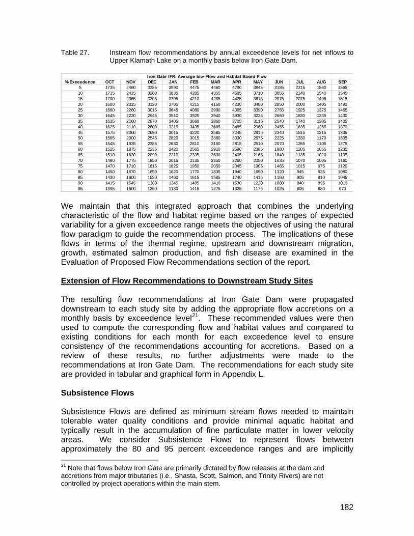
182
Table 27. Instream flow recommendations by annual exceedence levels for net inflows to Upper Klamath Lake on a monthly basis below Iron Gate Dam.
We maintain that this integrated approach that combines the underlying characteristic of the flow and habitat regime based on the ranges of expected variability for a given exceedence range meets the objectives of using the natural flow paradigm to guide the recommendation process. The implications of these flows in terms of the thermal regime, upstream and downstream migration, growth, estimated salmon production, and fish disease are examined in the Evaluation of Proposed Flow Recommendations section of the report. Extension of Flow Recommendations to Downstream Study Sites The resulting flow recommendations at Iron Gate Dam were propagated downstream to each study site by adding the appropriate flow accretions on a monthly basis by exceedence level21. These recommended values were then used to compute the corresponding flow and habitat values and compared to existing conditions for each month for each exceedence level to ensure consistency of the recommendations accounting for accretions. Based on a review of these results, no further adjustments were made to the recommendations at Iron Gate Dam. The recommendations for each study site are provided in tabular and graphical form in Appendix L. Subsistence Flows Subsistence Flows are defined as minimum stream flows needed to maintain tolerable water quality conditions and provide minimal aquatic habitat and typically result in the accumulation of fine particulate matter in lower velocity areas. We consider Subsistence Flows to represent flows between approximately the 80 and 95 percent exceedence ranges and are implicitly 21 Note that flows below Iron Gate are primarily dictated by flow releases at the dam and accretions from major tributaries (i.e., Shasta, Scott, Salmon, and Trinity Rivers) are not controlled by project operations within the main stem.
% Exceedence OCT NOV DEC JAN FEB MAR APR MAY JUN JUL AUG SEP5 1735 2460 3385 3990 4475 4460 4790 3845 3185 2215 1560 1565
10 1715 2415 3280 3835 4285 4355 4585 3710 3055 2140 1540 154515 1700 2365 3205 3795 4210 4285 4425 3615 2975 2075 1495 151520 1680 2315 3120 3705 4215 4160 4230 3480 2850 2000 1405 149025 1660 2260 3015 3645 4080 3990 4065 3390 2755 1925 1375 146530 1645 2220 2945 3510 3925 3940 3930 3225 2660 1830 1335 143035 1635 2160 2870 3405 3660 3860 3705 3115 2540 1740 1305 140540 1625 2110 2800 3215 3435 3685 3485 2960 2455 1635 1255 137045 1575 2060 2690 3015 3220 3585 3245 2815 2340 1515 1215 133550 1565 2000 2545 2820 3015 3380 3030 2675 2225 1330 1170 130555 1545 1935 2385 2630 2810 3150 2815 2510 2070 1265 1105 127560 1525 1875 2235 2420 2565 2910 2590 2385 1980 1205 1055 123565 1510 1830 2090 2210 2335 2630 2405 2165 1840 1135 1020 119570 1490 1775 1950 2015 2135 2350 2260 2050 1635 1070 1005 116075 1470 1710 1815 1825 1950 2050 2045 1905 1465 1015 975 112080 1450 1670 1650 1620 1770 1835 1940 1690 1320 945 935 108085 1430 1600 1520 1460 1615 1585 1740 1415 1160 905 910 104590 1415 1545 1380 1245 1485 1410 1530 1220 1080 840 895 101095 1395 1500 1260 1130 1415 1275 1325 1175 1025 805 880 970
Iron Gate IFR: Average b/w Flow and Habitat Based Flow

183
addressed by our flow recommendation process (see Base Flows section above). At these flow exceedence ranges, water temperature affects in terms of increased risk associated with thermal stress, disease, and migration inhibition become a concern. We believe that these conditions naturally occurred within the main stem Klamath River below Iron Gate Dam and they in fact represent an important environmental stressor for long-term population genetics and therefore have attempted to balance our recommendations between allowing the full range of natural flow and temperature conditions to exist and the objective to reduce these risks to acceptable levels. Ecological Base Flows One of the fundamental concepts that have evolved within the science of instream flows over the past two decades is that of an ‘Ecological Base Flow’ or EBF. Conceptually, the EBF represents a flow at which further human induced reductions in flow would result in unacceptable levels of risk to the health of the aquatic resources. Although this concept is understood and widely accepted by instream flow practitioners, no systematic quantitative research has been undertaken to define what an EBF would be for particular river systems and their unique flow dependent resources. However, available literature on instream flow assessments, drought management plans that incorporate ecological risk components, and some quantitative assessments of hydraulic properties from a number of river systems, suggest that a general rule-of-thumb for an EBF can be derived as discussed below. At present, three main efforts have been identified in which some form of an EBF was recognized to illustrate the current ‘state-of-the-art’. The first two approaches have evolved within instream flow assessment practices in Australia and South Africa. The third was developed within England in response to the European Union (EU) Water Framework Directive(s) to establish protection for aquatic resources within the EU. Queensland Environmental Flow Assessment Framework The fundamental basis for this approach is outlined in ‘Guidelines for Environmental Flow Management in Queensland Rivers’ (Brizga and Arthington 2001) that has subsequently been refined based on subsequent experiences. This is best characterized by the Pioneer Valley Water Resource Plan (State of Queensland, Department of Natural Resources and Mines, 2001). It reflects the current use of an environmental flow assessment framework required in the development of Water Resource Plans (WRPs) that set environmental flow objectives used to assess alternative water resource management scenarios. The approach relies on key flow indicators that are benchmarked against ‘acceptable’ levels of departure from natural flow conditions to set environmental flow objectives. This is undertaken within an established risk assessment framework.

184
The approach involves the delineation of key flow indicators based on geomorphologic and ecological functions of various aspects of the flow regime based on a review of existing information, general principles outlined in the scientific literature, and local knowledge of the systems. The methodology covers the full spectrum of inter and intra-annual flow variations. In terms of an EBF their focus on low flows centered on what is referred to as ‘Level 1 and Level 2’ risk categories that indicate flow characteristics that depart from natural conditions such that there is a higher likelihood that major or very major impacts would occur to geomorphologic and/or ecological conditions. Seven key flow indicators were proposed in the methodology of which two are particularly germane to the discussion of EBFs. They consider that departures on the order of +/- 10 to 20 percent from natural flows at the 80 to 90 percent daily exceedence durations of monthly flows to represent critical levels of risk. They further index increased risk associated with the daily exceedence duration for 10 cm depth of flow as a critical factor and this index should not depart more than +/- 10 to 20 percent of the natural flow regime. Use of the 10 cm depth criteria as an important index with ecological implications was derived from experiences in applying the South African Building Block Methodology (discussed below) (Arthington and Long 1997, Arthington and Lloyd 1998). Their experience in Australia suggested that flows that maintain at least 10 cm of depth over riffles and glides are indicative of normal functioning in these types of habitats, while reductions in the duration of 10 cm depth of flow are associated with increased areas of dewatering in these habitats more frequently than natural. They caveat their work by saying, “The disturbance represented by Level 1 or Level 2 in the risk assessment models represent levels of geomorphologic and ecological change which may be indicative of, but are not necessarily identical to, levels of degradation” (Arthington and Long 1997, Arthington and Lloyd 1998). Based on the level of uncertainty that is inherent with ecological risk assessment, they recommend setting of environmental flow objectives that are conservative. Although the risk assessment framework and specification of key flow indices recognize a number of methodologies, it basically relies on professional judgment in establishing the corresponding thresholds of key flow indicators, regardless of the methodology. In fact, they acknowledge that use of the 10 cm depth of flows, or 50, 80 and 90 percent daily exceedence durations “do not have any special intrinsic significance” (Arthington and Long 1997, Arthington and Lloyd 1998), but are used as indicators of flows in the very low flow ranges. Figure 144 illustrates their basic concept of how the low flow indicators are utilized based on an 80 percent daily exceedence duration flow (although they recommend using the 50 and 90 percent exceedence levels as better indicators of low flow change conditions).
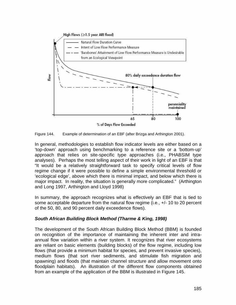
185
Figure 144. Example of determination of an EBF (after Brizga and Arthington 2001). In general, methodologies to establish flow indicator levels are either based on a ‘top-down’ approach using benchmarking to a reference site or a ‘bottom-up’ approach that relies on site-specific type approaches (i.e., PHABSIM type analyses). Perhaps the most telling aspect of their work in light of an EBF is that “It would be a relatively straightforward task to specify critical levels of flow regime change if it were possible to define a simple environmental threshold or ‘ecological edge’, above which there is minimal impact, and below which there is major impact. In reality, the situation is generally more complicated.” (Arthington and Long 1997, Arthington and Lloyd 1998) In summary, the approach recognizes what is effectively an EBF that is tied to some acceptable departure from the natural flow regime (i.e., +/- 10 to 20 percent of the 50, 80, and 90 percent daily exceedence flows). South African Building Block Method (Tharme & King, 1998) The development of the South African Building Block Method (BBM) is founded on recognition of the importance of maintaining the inherent inter and intra-annual flow variation within a river system. It recognizes that river ecosystems are reliant on basic elements (building blocks) of the flow regime, including low flows (that provide a minimum habitat for species, and prevent invasive species), medium flows (that sort river sediments, and stimulate fish migration and spawning) and floods (that maintain channel structure and allow movement onto floodplain habitats). An illustration of the different flow components obtained from an example of the application of the BBM is illustrated in Figure 145.
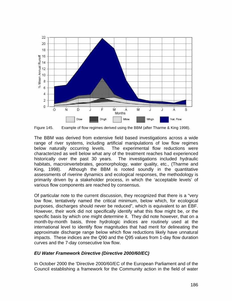
186
Figure 145. Example of flow regimes derived using the BBM (after Tharme & King 1998). The BBM was derived from extensive field based investigations across a wide range of river systems, including artificial manipulations of low flow regimes below naturally occurring levels. The experimental flow reductions were characterized as well below what any of the treatment reaches had experienced historically over the past 30 years. The investigations included hydraulic habitats, macroinvertebrates, geomorphology, water quality, etc., (Tharme and King, 1998). Although the BBM is rooted soundly in the quantitative assessments of riverine dynamics and ecological responses, the methodology is primarily driven by a stakeholder process, in which the ‘acceptable levels’ of various flow components are reached by consensus. Of particular note to the current discussion, they recognized that there is a “very low flow, tentatively named the critical minimum, below which, for ecological purposes, discharges should never be reduced”, which is equivalent to an EBF. However, their work did not specifically identify what this flow might be, or the specific basis by which one might determine it. They did note however, that on a month-by-month basis, three hydrologic indices are routinely used at the international level to identify flow magnitudes that had merit for delineating the approximate discharge range below which flow reductions likely have unnatural impacts. These indices are the Q90 and the Q95 values from 1-day flow duration curves and the 7-day consecutive low flow. EU Water Framework Directive (Directive 2000/60/EC) In October 2000 the 'Directive 2000/60/EC of the European Parliament and of the Council establishing a framework for the Community action in the field of water

187
policy' (EU Water Framework Directive or WFD) was adopted. The purpose of the Directive is to establish a framework for the protection of inland surface waters (rivers and lakes), transitional waters (estuaries), coastal waters and groundwater. It will ensure all aquatic ecosystems and, with regard to their water needs, terrestrial ecosystems and wetlands meet 'good status' by 2015. The Directive requires Member States to establish river basin districts and for each of these districts, a river basin management plan. The Directive envisages a cyclical process where river basin management plans are prepared, implemented and reviewed every six years. There are four distinct elements to the river basin planning cycle: characterization and assessment of impacts on river basin districts; environmental monitoring; the setting of environmental objectives; and the design and implementation of the program of measures needed to achieve them. “Development Of Environmental Standards: (Water Resources) Stage 3: Environmental Standards (2006)” prepared collaboratively by the Centre for Ecology & Hydrology, Environmental Systems Research Group at the University of Dundee and the Scotland and Ireland Forum for Environmental Research (SNIFFER) to specifically meet this EU mandate (SNIFFER 2006). Basically, the Water Framework Directive requires member states to achieve good ecological status (GES) in all surface and ground waters. GES is defined qualitatively as a slight deviation from the reference status, based on populations and communities of fish, macro-invertebrates, macrophytes and phytobenthos, and phytoplankton. They utilized experts on macrophytes, macro-invertebrates, fish and more general experts in river and lake management from the Environment Agency of England and Wales, Scottish Environment Protection Agency and Environment and the Heritage Service Northern Ireland. The experts felt strongly that insufficient knowledge was available to define precise generic environmental standards and therefore approached the definition of criteria from a precautionary approach by considering incrementally higher levels of flow alteration and deciding at what level of flow alteration that they could no longer be certain that GES would be achieved. Several key findings related to the discussion of an EBF were, however, obtained. In general, standards should be specified in terms of deviations from the natural flow regime. With some variations for specific resources (e.g. macrophytes), flow regimes should be within about 20 percent of natural to achieve GES. This is consistent with English Nature flow targets of 10 percent abstraction for rivers designated as Special Areas of Conservation (SACs) under the Habitats Directive, which is broadly equivalent to maintaining a high level of protection. When a precautionary approach is warranted for restrictive management, there was wide support given for the idea of preserving the Q95 flow by designating this as a “hands-off” flow. The concept being that when the river flow drops to and below Q95, abstraction either stops or is significantly reduced.

188
Quantitative Assessment of Flow Reductions A project is currently underway between the Centre for Ecology & Hydrology and Utah State University, jointly funded by the Centre for Ecology and Hydrology and the Environment Agency (England), entitled Rapid Assessment of Physical Habitat Sensitivity to Abstraction (RAPHSA). The RAPHSA database contains 65 river sites at which detailed hydraulic data have been collected to undertaken habitat modeling studies, such as PHABSIM. These hydraulic data were used to study the impact of flow changes on the physical character of river channels. Each of the 65 RAPHSA sites was analyzed to identify break points in these relationships. At many sites the relationship took the form of a smooth curve with no obvious break point; however, threshold points were identified at 36 sites. The range of break points is shown in Figure 146. It can be seen that the model value is around Q95 with a mean of Q92. No obvious relationship was found between threshold level and river site type.
Figure 146. Relationship between flow exceedence level and rate of habitat change (after Acreman et al., 2006).
This analysis suggests that Q95 marks a significant point below which conditions in the river change rapidly and hence the river is more sensitive to flow change. These results provided additional justification for hands-off flows at Q95 in restrictive management and maintaining Q95 in active management for the Development of Environmental Standards project discussed above. Based on these efforts and analyses, we have adopted an Ecological Base Flow that is equivalent to the monthly 95 percent exceedence levels. Note that the EBF recommendations are derived from the lower bound of the expected 90th percentile range below the mean flow at this exceedence level (see the Base Flow section above). Additional justification of these flow regimes are provided in the following sections of the report.
02468
10121416
84 86 88 90 92 94 96 98
threshold percentile
num
ber
of s
ites
189
Evaluation and Justification of Proposed Flow Recommendations The proposed instream flow recommendations were evaluated using a number of analyses in order to provide the ecological justification for these flows. This included use of SIAM to compare expected salmon production estimates; travel time and thermal refugia encounter rates, and bioenergetic-based modeling of expected fish growth. These assessments were used to compare our recommendations against existing conditions in light of existing empirical data and supporting scientific literature. As part of this evaluation, we also document expected affects of the proposed flow recommendations on system operations in terms resulting Upper Klamath Lake elevations and potential impacts to out-of-stream water deliveries. Anadromous Use of the Main Stem and the Thermal Regime Extensive documentation has been produced by a number of researchers and management agencies that show the thermal regime under historical and existing conditions below Iron Gate Dam downstream to below Seiad Valley can be thermally hostile to anadromous salmonids, especially during the summer and early fall period. Our draft recommendation of ~ 1,000 cfs as a summer floor was based on the belief that the ecological risk of thermal related limiting factors (i.e., disease, migration barriers) increases as flows incrementally drop below about this flow magnitude. Fundamentally, we believe that the key to understanding the potential implications of our proposed flow regime centers on the physical limitations imposed by temperature dependent pokilotherm physiology and their behavioral based mechanisms of thermoregulation. Our flow recommendations were used to estimate the temperature regimes downstream of Iron Gate Dam using SIAM and supplemented with inferences that can be made based on temperature modeling using the RMA-2/11 results for the without project conditions. In addition, we have incorporated field observations on thermal refugia use and evaluate these data in light of the implications of our proposed flow regimes. High river temperatures in the tributaries and main stem Klamath River have been implicated in controlling salmonid use of the main stem river (e.g., see Bartholow 2005, Bartholow et al., 2005, NRC 2004, Dunsmoor and Huntington 2006). Temperatures in the lower main stem Klamath River below Iron Gate Dam during the summer and early fall are frequently in the range of 22-26+°C. These temperatures are well within the range of temperatures that can produce acute death, chronic weight loss and mortality, increased disease incidence and mortality, predation mortality, blockage of migration, and impaired smoltification for salmonids (e.g., see reviews by Sullivan et al., 2000, Myrick and Cech 2001, USEPA 2003).

190
Direct mortality has been observed in the main stem linked to temperature and disease. For example, dead fish were observed while sampling near Happy Camp in 1997 when water temperatures were 26.7°C (Tom Shaw, USFWS, personal communication). In September 2002 a large fish kill occurred as a combination of high fish numbers, low flows, high temperature, and disease (USFWS 2003a/b, CDFG 2004). The lower main stem Klamath River is nearly 200 miles long and is used as an adult migration corridor to upstream main stem spawning, holding, and tributary spawning locations. It is used both as a dispersal corridor for fry and juveniles and as an out migration corridor by juveniles/smolts. It is also used for rearing habitat by Chinook fry and juveniles, steelhead fry and juveniles, and coho fry and juveniles but at reduced densities for this species in July and August during peak main stem temperatures. Anadromous salmonid adults, juveniles, fry, and/or eggs are present in the lower main stem throughout every month of the year. During the summer and early fall high temperature period, juvenile and migrating adult salmonids (steelhead, Chinook and coho salmon) frequently utilize temperature refugia as a behavioral thermoregulation strategy (Deas et al., 2006, Belchik 1997, 2003). Temperature refugia consist of tributary streams (~ 126 streams), tributary inflow plumes to the main stem Klamath River, and hyporheic flows within the riverbed. NRC (2004, Page 257) citing to unpublished data from McIntosh and Li (1998) using thermal imaging from the Klamath River main stem, suggest that ‘pools apparently are the only cool-water refugia in the river and occupy only a small area’. However, Tanaka et al., (2006) used thermal imaging within the main stem Klamath River as part of field studies on thermal refugia responses to flow and meteorological variations and found that the imagery was not capable of detecting near bed hyporheic flows. Tanaka et al., (2006) report differences in water temperatures between the near bed and water surface of 7.7°C not indicated by the thermal imagery and conclude, “refugial areas influenced by subsurface flow may provide additional thermal habitat that would be underrepresented using aerial thermal imagery based on surface water temperatures”. Another interesting finding in Tanaka et al., (2006) is that the diel pattern of subsurface temperatures was out of phase by approximately 12 hours with the main stem Klamath River at their study site. This means that the subsurface flows are at their lowest when the main stem river is at its maximum daily temperature. This would coincidentally provide access to the lowest temperatures during the period when the main stem is most hostile. They also conclude from their empirical data that under existing channel conditions, flows as high as ~ 1300 cfs did not substantially alter the characteristics of the thermal refugia studied. This flow range is at the upper limit of the July and August recommended flows for exceedence levels of > 50 percent. We therefore conclude that our recommended flows do not represent a significant risk to degrading thermal refugia over these flow ranges. We believe that more extensive hyporheic flows are present within the main stem Klamath
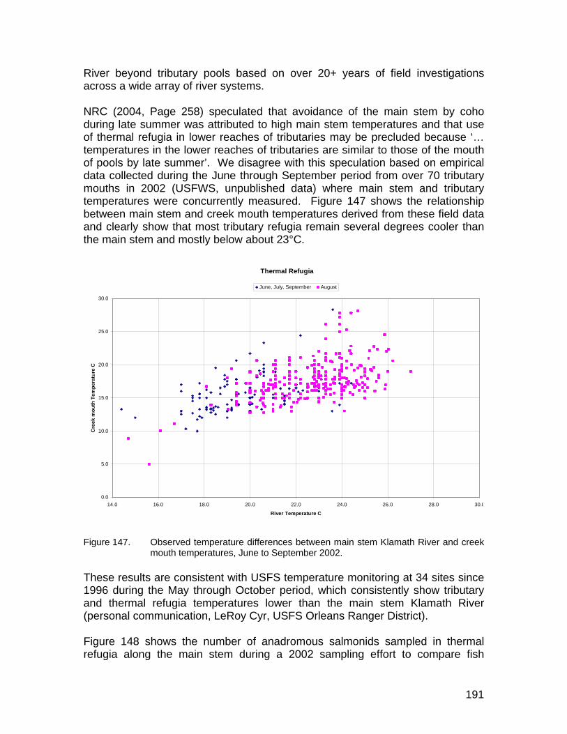
191
River beyond tributary pools based on over 20+ years of field investigations across a wide array of river systems. NRC (2004, Page 258) speculated that avoidance of the main stem by coho during late summer was attributed to high main stem temperatures and that use of thermal refugia in lower reaches of tributaries may be precluded because ‘… temperatures in the lower reaches of tributaries are similar to those of the mouth of pools by late summer’. We disagree with this speculation based on empirical data collected during the June through September period from over 70 tributary mouths in 2002 (USFWS, unpublished data) where main stem and tributary temperatures were concurrently measured. Figure 147 shows the relationship between main stem and creek mouth temperatures derived from these field data and clearly show that most tributary refugia remain several degrees cooler than the main stem and mostly below about 23°C.
Figure 147. Observed temperature differences between main stem Klamath River and creek
mouth temperatures, June to September 2002. These results are consistent with USFS temperature monitoring at 34 sites since 1996 during the May through October period, which consistently show tributary and thermal refugia temperatures lower than the main stem Klamath River (personal communication, LeRoy Cyr, USFS Orleans Ranger District). Figure 148 shows the number of anadromous salmonids sampled in thermal refugia along the main stem during a 2002 sampling effort to compare fish
Thermal Refugia
0.0
5.0
10.0
15.0
20.0
25.0
30.0
14.0 16.0 18.0 20.0 22.0 24.0 26.0 28.0 30.0
River Temperature C
Cre
ek m
outh
Tem
pera
ture
C
June, July, September August

192
numbers in temperature refugia (unpublished data USFWS). These data show that significant numbers of fish are associated with temperature refugia locations. Excursions into this temperature range can be accommodated for brief periods with the time of exposure dependent upon thermal acclimation history and characteristics (i.e., constant versus fluctuating) (see Temperature and Bioenergetics section below).
Figure 148. Summer fish sampling in the main stem Klamath River in temperature refugia
locations. The highest temperatures were in July and August. The total number of fish in the plot is 60,680 (See Table 28).
Table 28 shows the 2002 monthly counts of salmonids, by species and life stage, that were observed in the thermal refugia areas of the main stem Klamath River. (USFWS unpublished data). These data clearly show a reduction in main stem numbers after July but also document Chinook, steelhead, and coho use of the main stem and associated refugia continuously through the summer period.
Main Stem Klamath River June through mid-September 2002Chinook Fry/Juvenile Coho Fry/Juvenile Steelhead Fry/1+
0.0
200.0
400.0
600.0
800.0
1000.0
1200.0
1400.0
1600.0
1800.0
2000.0
10.0 12.0 14.0 16.0 18.0 20.0 22.0 24.0 26.0 28.0
Temperature C
Tota
l Num
bers
of A
ndom
ous
Fry/
Juve
nile
s

193
Table 28. Monthly counts of anadromous fish observed in the main stem Klamath River within thermal refugia areas during 2002 (USFWS unpublished data).
Chinook 0+ Coho 1+ Coho 0+ Steelhead 1+
Steelhead 2+ and Half Pounders Total
Percent of Total
June 3955 50 184 1493 319 6001 9.89 July 11997 1 155 24676 3288 40117 66.11 August 3155 6 57 7800 2988 14006 23.08 September 213 0 15 236 92 556 0.92 Observations of fish use at temperatures above 22°C and as high as 26°C are supported by the literature on thermal regulation that demonstrate fish acclimated to fluctuating conditions (i.e., real world conditions) can tolerate excursions into temperatures of this magnitude for brief periods. We believe, however, that the existing thermal refugia work cited above clearly demonstrate behavioral thermoregulation strategies for all the anadromous species considered and show increasing use of thermal refugia when main stem water temperatures approach approximately 22°C. This is further supported by field observations in the Salmon River (Tom Shaw, personnel communication) that show outmigration of smolts stopped when water temperatures approached ~22°C and then resumed when a cool front passed and water temperatures were reduced below this threshold. NRC (2004) utilized simulated water temperatures based on Deas (2000) to postulate that the declining use of tributary thermal refugia by coho in July and August was attributed to the temperatures in the main stem that were, from a bioenergetic perspective, higher than what coho would be expected to tolerate. We believe this reduction in use and avoidance of the main stem by coho is in fact reflected in our species periodicity chart where June is identified as a low use month and by July they are considered generally absent from the main stem system (see Table 15). NRC (2004) also highlighted the continual use of main stem thermal refugia by Chinook and steelhead throughout the summer period consistent with their higher thermal tolerances (NRC, Page 257, Table 7-3) and is reflective of the empirical data provided in Table 28. Implications of Recommended Flows on the Thermal Regime Simulation results from Deas (2000) were used in the draft report and by NRC (2004) to illustrate that as flow increases below Iron Gate Dam, the travel time decreases. This results in a dampening in the range of daily temperature variation and a downstream shift in the locations of the node of minimum diel temperature variation (~24 hour travel time) and an antinode of maximum diel temperature variation (~12 hour travel time). Figure 149 shows these relationships for flows between 600 to 3000 cfs at Iron Gate at an expected release temperature of ~ 22.0°C for typical August conditions.

194
Figure 149. Simulated minimum, mean, and maximum daily water temperatures for a typical
August period in the main stem Klamath River below Iron Gate Dam downstream to Seiad Valley (data from Deas (2000), used with permission). Vertical lines denote location of key tributaries with the average August flow rate (cfs) indicated above the name.
NRC (2004) utilized these data to illustrate conditions at 1000 and 3000 cfs (NRC 2004, Page 150) and to opine that although increasing flows may reduce the mean and maximum daily temperatures, the increase in minimum daily temperatures ‘may adversely affect fish [coho] that are at their limits of thermal tolerance’ and that flow releases of 3000 cfs would eliminate any benefit [temperature - for coho] from tributary accretions citing Deas (2000)22. An examination of the flow recommendations in Table 27 for exceedence between 95 and 50 percent range from approximately 800 to 1300 in the July/August period and that an increase in the daily minimum temperatures are on the order of 1°C over this entire flow range. Deas and Orlob (1999) modeling results based on RMA for the Klamath River below Iron Gate Dam demonstrate that increased flows would result in slightly cooler temperatures in the main stem Klamath River (e.g., a difference of 1°C cooler from 500 cfs to 1,000 cfs) and that 22 Note that a flow of 3000 cfs in August corresponds to an exceedence level of less than 5 percent based on either the BOR Natural Flow or Consumptive Use estimates and therefore not relevant to the actual issue of potential thermal affects.
Longitudinal Maximum and Minimum Water Temperature Profiles:600-3000 cfs (8/14/96)
Willow7.7
Cottonwood13
Shasta63
Humbug15.5
Beaver16.1
Dona2
Horse11.1
Scott111.5
Walker12.5Bogus
14.4
16.0
17.0
18.0
19.0
20.0
21.0
22.0
23.0
24.0
25.0
26.0
27.0
28.0
129132135138141144146149152155158161164167170173176179181184187190
River Mile
Tem
pera
ture
(°C
)
-80
-60
-40
-20
0
20
40
60
80
Tributaries 600 cfs 700 cfs 800 cfs 900 cfs 1000 cfs 1100 cfs 1200 cfs 1300 cfs 1400 cfs 1500 cfs 3000 cfs
195
the increased flows would not increase river temperature. We examine the biological implications of our flow recommendations in more detail in the next section. NRC (2004) further opine that increasing the flow during this period might be somewhat harmful to coho but could favor other anadromous species that rely on the main stem during this period. They also note that ‘the ability of steelhead to thrive under the summer temperatures in the lower Klamath … [that steelhead] … will benefit from the expansion of habitat created by increased flows in the mainstem Klamath and tributaries, as long as water quality, especially temperature, remains suitable for them’. NRC (2004) concludes that ‘from a bioenergetics perspective, increasing minimum temperatures may be especially unfavorable for coho in the main stem because nocturnal relief from high temperatures would be reduced’ (NRC 2004, Page 259). Using bioenergetic principals, they concluded that the existing thermal regime in the main stem Klamath precluded it as coho fry or juvenile habitat from approximately late June to early October. We postulate a different view of the bioenergetic importance of raising the minimum daily water temperature on rearing salmonids (e.g., Chinook and steelhead) below Iron Gate Dam under recommended flow regimes than that proffered by NRC (2004). We provide data below that show changes in the magnitude and range of the maximum and mean daily temperatures are better indicators of assessing bioenergetic-based responses in growth below the upper acute thermal limit. Analyses are also presented on potential growth under existing and proposed flow recommendations that support our view. The NRC (2004) stressed the importance of protecting and enhancing tributary conditions for coho rearing and we believe that ultimate recovery of coho and enhancement of all anadromous stocks that rely on the main stem Klamath River is in part contingent on properly functioning tributary systems. The Phase II recommendations target other anadromous species and life stages during late June through the early fall period that are known to inhabit the river such as fry and juvenile of Chinook and steelhead and critically dependent seasonally on these tributary inflows. NRC (2004) also note that limiting factors controlling the survival of Chinook fry in the main stem is not known especially given abundant food supplies and summer temperatures that although are potentially stressful, are rarely lethal. They postulate that increasing flows to increase edge habitat for small fish (i.e., Chinook and steelhead rearing life stages) at the stream margin for feeding and predator avoidance would be desirable for as long as small fish are present. Our flow recommendations embody this view based on the use of our physical habitat modeling for fry that stressed the importance of edge habitat associated with escape cover.

196
Temperature and Bioenergetics A list of general temperature criteria for anadromous salmonids developed by the Region 10 Environmental Protection Agency (EPA) is provided in Table 29 (EPA 2003). The EPA temperature review was comprehensive. In addition, to a report highlighting the recommended temperature criteria, several issue papers were developed during the review process that elaborated on details of the literature review and the logic for the temperature criteria. In general, we endorse and refer to the EPA temperature criteria (EPA 2003) and associated issue papers used to develop the criteria. Here, however, we highlight a few important observations relative to the acute temperature criteria because of the frequency that temperatures near the acute range occur in the Lower Klamath River. We also attempt to clarify what appears to be a misperception regarding bioenergetics and the effect of diel temperature fluctuations that exists in some recent reports (NRC 2004, Dunsmoor and Huntington 2006). Myrick and Cech (2001) provide an excellent introduction to the literature on methodologies employed to estimate thermal preference and tolerance limits. They draw attention to the inherent consequence of the acclimation regime (i.e., constant versus variable) employed in the methodology and the specific types of testing method (e.g., CTM or ILT) have on study results and their implication on interpretation. They also introduce thermal niche limits for salmonids that incorporate behavioral avoidance ranges versus acclimation temperature and is consistent with our discussion of realized niches under habitat suitability curves. Acute temperature maximums are very similar for many salmonids (EPA Issue Paper 5, Lee and Rinne 1980). Upper incipient lethal temperatures (UILT) for juvenile Chinook salmon, coho salmon, and rainbow trout are 25 to 26°C. Redband trout seem to have a slightly higher UILT, as high as 27°C. Adult salmonid UILTs are 2 to 3°C lower than the UILTs for juveniles (e.g., 22°C) (EPA Issue Paper 5). Fish stop feeding at a temperature slightly less (e.g., 1-2°C) than the UILT (EPA Issue Paper 5). The UILT is the temperature at which 50 percent of the fish (acclimated to a high temperature) can survive for a fixed amount of time (1000 min to 7 days depending on the investigator). The length of exposure to high temperature is an important variable in determining the UILT. Fish can withstand higher temperatures for a shorter period of time and lower high temperatures for a longer period of time. However, because the effects of repeated high temperature exposure are cumulative, peak daily temperatures in the Klamath River that reach the UILT likely cause some level of mortality. Peak daily temperatures less than 22 – 24°C are likely required to eliminate acute mortality (see Hokanson et al., 1977, EPA Issue Paper 5, page 88).
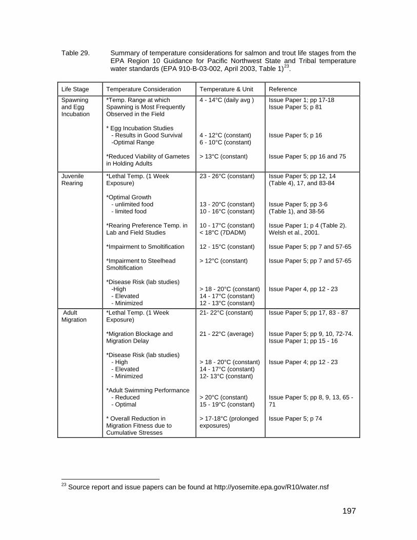
197
Table 29. Summary of temperature considerations for salmon and trout life stages from the EPA Region 10 Guidance for Pacific Northwest State and Tribal temperature water standards (EPA 910-B-03-002, April 2003, Table 1)23.
Life Stage Temperature Consideration Temperature & Unit Reference
Spawning and Egg Incubation
*Temp. Range at which Spawning is Most Frequently Observed in the Field * Egg Incubation Studies - Results in Good Survival -Optimal Range *Reduced Viability of Gametes in Holding Adults
4 - 14°C (daily avg ) 4 - 12°C (constant) 6 - 10°C (constant) > 13°C (constant)
Issue Paper 1; pp 17-18 Issue Paper 5; p 81 Issue Paper 5; p 16 Issue Paper 5; pp 16 and 75
Juvenile Rearing
*Lethal Temp. (1 Week Exposure) *Optimal Growth - unlimited food - limited food *Rearing Preference Temp. in Lab and Field Studies *Impairment to Smoltification *Impairment to Steelhead Smoltification *Disease Risk (lab studies) -High - Elevated - Minimized
23 - 26°C (constant) 13 - 20°C (constant) 10 - 16°C (constant) 10 - 17°C (constant) < 18°C (7DADM) 12 - 15°C (constant) > 12°C (constant) > 18 - 20°C (constant) 14 - 17°C (constant) 12 - 13°C (constant)
Issue Paper 5; pp 12, 14 (Table 4), 17, and 83-84 Issue Paper 5; pp 3-6 (Table 1), and 38-56 Issue Paper 1; p 4 (Table 2). Welsh et al., 2001. Issue Paper 5; pp 7 and 57-65 Issue Paper 5; pp 7 and 57-65 Issue Paper 4, pp 12 - 23
Adult Migration
*Lethal Temp. (1 Week Exposure) *Migration Blockage and Migration Delay *Disease Risk (lab studies) - High - Elevated - Minimized *Adult Swimming Performance - Reduced - Optimal * Overall Reduction in Migration Fitness due to Cumulative Stresses
21- 22°C (constant) 21 - 22°C (average) > 18 - 20°C (constant) 14 - 17°C (constant) 12- 13°C (constant) > 20°C (constant) 15 - 19°C (constant) > 17-18°C (prolonged exposures)
Issue Paper 5; pp 17, 83 - 87 Issue Paper 5; pp 9, 10, 72-74. Issue Paper 1; pp 15 - 16 Issue Paper 4; pp 12 - 23 Issue Paper 5; pp 8, 9, 13, 65 - 71 Issue Paper 5; p 74
23 Source report and issue papers can be found at http://yosemite.epa.gov/R10/water.nsf

198
The high temperature where positive growth ceases is also very similar for many salmonids if fed maximum ration on high quality food. The temperature where growth ceases is an important indicator of negative environmental temperature conditions. When fed to satiation (e.g., fed every hour), rainbow trout have positive growth up to a temperature of approximately 24°C (From and Rassmussen 1984, Sullivan et al., 2000), Chinook salmon have positive growth up to approximately 25°C (Brett et al., 1982), coho salmon have positive growth up about 24°C (Stewart and Ibarra 1991, Hanson et al., 1997, Sullivan et al., 2000), and brown trout have positive growth up to 20+°C (Elliott 1975). The availability of food makes a large difference in the highest temperature at which can achieve positive growth (e.g., Brett et al., 1992) (note: the activity level of a fish can also make a difference in the maximum temperature for positive growth). When less food is available, the temperature where growth ceases is lower. For example, if food consumption is 30 to 60 percent of maximum consumption, the temperature where growth ceases is 18 to 21°C (e.g., Brett et al 1982, Hanson 1997, Sullivan et al., 2000). Sullivan et al., (2000) developed widely differing 7-day maximum bioenergetics temperature criteria for coho salmon versus rainbow trout based on differences in assumed food consumption. The primary difference between a 20.5°C 7-day maximum temperature recommendation for coho versus a 24°C 7-day maximum temperature recommendation for rainbow trout (see page 7-7 in Sullivan et al., 2000) was the result of an approximately a 50 percent difference in assumed percent of maximum consumption between the two fish (the percents of maximum consumption were based on a limited empirical data set). To our knowledge, there has not been any work done to calculate the percent of maximum consumption that juvenile salmonids are achieving in the Lower Klamath River; thus, it is not possible to determine the maximum temperature at which juvenile fish can maintain positive growth. Addley et al., (2005) found that small rainbow trout (less than about 300 mm) achieved about 68-73 percent of maximum consumption in a hydropeaking reach of the Klamath River upstream of Iron Gate and the Copco Reservoirs. These results were obtained using the laboratory data of From and Rasmussen (1984) modified for invertebrate consumption by reducing the maximum consumption 50 percent (see Addley 2006). Using the From and Rasmussen (1984) results without modification based on a high calorie diet and hourly feeding, the percent of maximum consumption would have been 34-37 percent. Model results showed that fish less than about 200 mm could achieve positive growth at temperatures as high as approximately 22.5°C based on drift densities from 2 to 10+ prey/m3 (approximately the summer drift density in the lower Klamath River). We assume that approximately a similar situation exists for juvenile salmonids in the Lower Klamath River. The effect of high temperature on bioenergetics (growth) is time dependent. In a system with high summer temperatures, fish can grow well during the early late
199
spring/early summer, lose weight during the short period of the summer and then regain weight during the fall. The duration of the high temperatures determines the total weight loss (e.g., Addley et al., 2005). In the Modeled Growth section below, we estimate the growth of a juvenile Chinook salmon from early March through July using the equations in the Wisconsin Bioenergetics Model (Hanson et al., 1997) and juvenile steelhead for two plus years using the approach of Addley (2006). In a diel fluctuating temperature regime, the equivalent daily temperature at which fish respond bioenergetically (i.e., fish mean temperature) is a temperature between the mean daily temperature and the maximum daily temperature. There are very few comprehensive comparisons in the literature illustrating the effects of both steady temperatures and diel temperature fluctuations on bioenergetics (e.g., studies of growth over a wide range of temperatures with steady and fluctuating temperatures). Hokanson et al., (1977) and Cox and Coutant (1981) provide some of the best data. These data show that fish in fluctuating temperatures regimes grow at a temperature equivalent to the daily mean temperature plus some percent of the difference between the mean and the maximum. In Hokanson et al., (1977) the “fish mean” temperature was the daily mean temperature plus 40 percent of the difference between the daily maximum and mean temperature. There is also some evidence from other studies that daily mean temperature can be used to closely approximate the temperature exposure of salmonids in fluctuating temperature regimes (e.g., Elliott 1975). Some (e.g., Bjornn and Reiser 1991, NRC 2004, Dunsmoor and Huntington 2006) have inferred that cool nighttime temperature (the diel minimum temperature) by itself is an important attribute of an acceptable temperature regime. Here we try to clarify what we believe the existing temperature studies (literature) show in this regard. In the situation where fish are wholly confined in a high temperature regime (e.g., fish in the main stem Klamath River without nearby temperature refugia), the greater the diel fluctuations the more damaging the temperature regime is to the growth of the fish if the “fish mean” temperature is greater than the optimum temperature for growth (note that the optimum temperature depends on food availability). Greater diel fluctuations will result in correspondingly lower low temperatures, but higher high temperatures. Because the fish will grow at approximately the daily fish mean temperature (daily mean plus 40 percent of the difference between the mean and the maximum) (e.g., Hokanson et al., 1977, Cox and Coutant 1981), the high fluctuating regime will impair growth. In the case where fish are wholly confined in a hostile high temperature regime, bioenergetically the best option is to lower the daily mean and/or reduce diel temperature fluctuations so the fish mean temperature is reduced (irrespective of the daily minimum temperature). We can only speculate, for example that NRC (2004) assumed that diel minimum temperatures are an important attribute to coho juveniles based on the results of Bisson et al., (1988) that showed coho were able to exist in warm Mt. St. Helens streams (see discussion in NRC 2004) because the daily minimum temperatures were low. In

200
Bisson et al., (1988) the mean temperature was about 18°C (fish mean based on Hokanson et al., 1977 was about 21°C) and there was apparent high food abundance (see discussion of growth curves and food abundance/quality). This is an acceptable temperature under high food consumption. The daily minimum temperatures in this case were likely important primarily in the sense that they affected the mean daily temperature. Alternatively, if fish have access to daytime temperature refugia (e.g., tributary inflow plume, hyporheic flows) and can enter the cooler main stem water at night and in the morning when it is cooler, it is very possible that cool nighttime temperatures could be utilized to a bioenergetic advantage. Existing empirical data from the Klamath on thermal refugia use by anadromous species suggests that fish move into thermal refugia when main stem temperatures approach approximately 22°C (Deas et al., 2006, Belchik 1997,2003; Tanaka et al., 2006). Modeled Fish Growth Bioenergetics models were used to illustrate the relative effect of temperature on growth of Chinook salmon and steelhead in the Klamath River for different temperature regimes. For both Chinook salmon and steelhead, growth was modeled for daily river temperatures at locations below Iron Gate Reservoir, Seiad, and Orleans. The daily temperatures used were the “fish mean” (discussed above, e.g., Hokanson et al., 1977) for the Existing Conditions, Without Project (see Dunsmoor and Huntington 2006), and our flow recommendations. Chinook Chinook fry/juvenile growth was modeled with the Wisconsin Bioenergetics Model (Hanson et al., 1997, Stewart and Ibarra 1991) and used by approximately calibrating the percent of maximum consumption (P value) to the observed growth of fish sampled in the river between Iron Gate Reservoir and the confluence with the Shasta River (Tom Shaw, USFWS, unpublished data). Sample data from 1998 were used to estimate a P value of 0.415 (41.5 percent). The 0.415 P value was then used to approximate growth for each of the temperature scenarios. The default values in the Wisconsin Model Chinook salmon input files were used. In these model runs, Chinook salmon growth was started at 0.7 grams (40.5 mm) on March 14 for the Existing Conditions and our instream flow recommendations. This was based on empirical sample data (Figure 150) (Tom Shaw, USFWS, unpublished data). The model runs for the “unimpaired” conditions started growth a week earlier because temperatures for the “unimpaired” conditions scenario warm up approximately a week sooner (see Dunsmoor and Huntington 2006).

201
Figure 150. Empirical data for Chinook salmon growth in the main stem Klamath River below
Iron Gate Dam (USFWS unpublished data). Figures 151 to 154 show the simulated growth results for Chinook under each of the flow scenarios evaluated at Iron Gate, Seiad, and Orleans for simulated conditions during 2000, 2001, 2002, and 2003. Overall, predicted growth of Chinook is slightly higher than under existing conditions through about mid-May at all three study sites during all four years simulated. The simulations also clearly reflect the impacts of the different thermal regimes between years as reflected by up to a 2-3 week shift in the point at which no growth occurs. Prior to reaching these points of zero growth (due to high temperature), we speculate that Chinook would likely be actively engaged in behavioral thermoregulation and move downstream or into thermal refugia. It is interesting to note that these results generally reflect the outmigration timing of chinook (non-hatchery releases) from screw trap data (USFWS, unpublished data). Although the apparent differential in growth between the flow recommendations and existing conditions appear small, the fact that Chinook achieve a larger size sooner reduces predation risk and it is well established that larger smolts are associated with higher survival rates in the estuary. The results also suggest that by the time zero growth occurs, regardless of which flow scenario is considered, that beginning sometime around mid-May to mid-June depending on the water year and temperature, Chinook numbers within the upper river should decline and is, in fact, reflected in the fish numbers within these reaches as the summer progresses (Tom Shaw, personal communication, NRC 2004).
Model Calibration - Chinook
20
30
40
50
60
70
80
90
2/24 3/6 3/16 3/26 4/5 4/15 4/25 5/5 5/15 5/25 6/4 6/14
Date
Fish
Len
gth,
mm
Observed 1998 Predicted

202
Figure 151. Estimated weight and length of Chinook below Iron Gate, Seiad, and Orleans for
2000 based on application of the Wisconsin bioenergetics model (see text for description).
Estimated Chinook Growth: Iron Gate (2000)
30
40
50
60
70
80
3/5 3/25 4/14 5/4 5/24 6/13
Date
Leng
th, m
m
0
1.2
2.4
3.6
4.8
6
Wei
ght,
gram
s
Length: EC Length: WOP Length: IFR
Weight: EC Weight: WOP Weight: IFR
Estimated Chinook Growth: Seiad (2000)
30
40
50
60
70
80
3/5 3/25 4/14 5/4 5/24 6/13
Date
Leng
th, m
m
0
1.2
2.4
3.6
4.8
6
Wei
ght,
gram
sLength: EC Length: WOP Length: IFR
Weight: EC Weight: WOP Weight: IFR
Estimated Chinook Growth: Orleans (2000)
30
40
50
60
70
80
3/5 3/25 4/14 5/4 5/24 6/13
Date
Leng
th, m
m
0
1.2
2.4
3.6
4.8
6
Wei
ght,
gram
s
Length: EC Length: WOP Length: IFR
Weight: EC Weight: WOP Weight: IFR
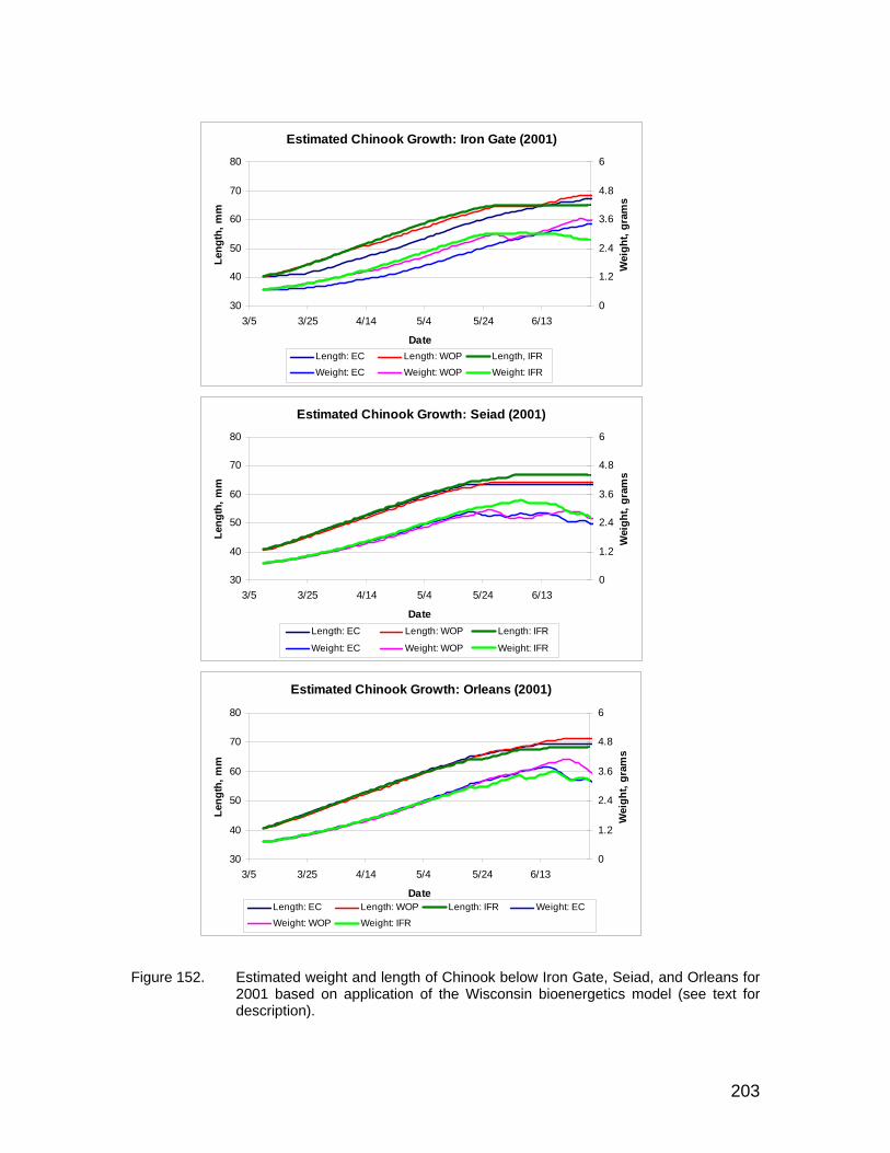
203
Figure 152. Estimated weight and length of Chinook below Iron Gate, Seiad, and Orleans for
2001 based on application of the Wisconsin bioenergetics model (see text for description).
Estimated Chinook Growth: Iron Gate (2001)
30
40
50
60
70
80
3/5 3/25 4/14 5/4 5/24 6/13
Date
Leng
th, m
m
0
1.2
2.4
3.6
4.8
6
Wei
ght,
gram
s
Length: EC Length: WOP Length, IFR
Weight: EC Weight: WOP Weight: IFR
Estimated Chinook Growth: Seiad (2001)
30
40
50
60
70
80
3/5 3/25 4/14 5/4 5/24 6/13
Date
Leng
th, m
m
0
1.2
2.4
3.6
4.8
6
Wei
ght,
gram
sLength: EC Length: WOP Length: IFR
Weight: EC Weight: WOP Weight: IFR
Estimated Chinook Growth: Orleans (2001)
30
40
50
60
70
80
3/5 3/25 4/14 5/4 5/24 6/13
Date
Leng
th, m
m
0
1.2
2.4
3.6
4.8
6
Wei
ght,
gram
s
Length: EC Length: WOP Length: IFR Weight: EC
Weight: WOP Weight: IFR

204
Figure 153. Estimated weight and length of Chinook below Iron Gate, Seiad, and Orleans for
2002 based on application of the Wisconsin bioenergetics model (see text for description).
Estimated Chinook Growth: Iron Gate (2002)
30
40
50
60
70
80
3/5 3/25 4/14 5/4 5/24 6/13
Date
Leng
th, m
m
0
1.2
2.4
3.6
4.8
6
Wei
ght,
gram
s
Length: EC Length: WOP Length: IFR
Weight: EC Weight: WOP Weight: IFR
Estimated Chinook Growth: Seiad (2002)
30
40
50
60
70
80
3/5 3/25 4/14 5/4 5/24 6/13
Date
Leng
th, m
m
0
1.2
2.4
3.6
4.8
6
Wei
ght,
gram
sLength: EC Length: WOP Length: IFR
Weight: EC Weight: WOP Weight: IFR
Estimated Chinook Growth: Orleans (2002)
30
40
50
60
70
80
3/5 3/25 4/14 5/4 5/24 6/13
Date
Leng
th, m
m
0
1.2
2.4
3.6
4.8
6
Wei
ght,
gram
s
Length: EC Length: WOP Length: IFR
Weight: EC Weight: WOP Weight: IFR
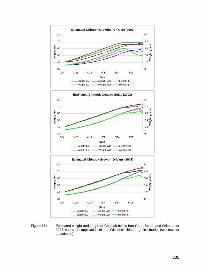
205
Figure 154. Estimated weight and length of Chinook below Iron Gate, Seiad, and Orleans for
2003 based on application of the Wisconsin bioenergetics model (see text for description).
Estimated Chinook Growth: Iron Gate (2003)
30
40
50
60
70
80
3/5 3/25 4/14 5/4 5/24 6/13
Date
Leng
th, m
m
0
1.2
2.4
3.6
4.8
6
Wei
ght,
gram
s
Length: EC Length: WOP Length: IFR
Weight: EC Weight: WOP Weight: IFR
Estimated Chinook Growth: Seiad (2003)
30
40
50
60
70
80
3/5 3/25 4/14 5/4 5/24 6/13
Date
Leng
th, m
m
0
1.2
2.4
3.6
4.8
6
Wei
ght,
gram
sLength: EC Length: WOP Length: IFR
Weight: EC Weight: WOP Weight: IFR
Estimated Chinook Growth: Orleans (2003)
30
40
50
60
70
80
3/5 3/25 4/14 5/4 5/24 6/13
Date
Leng
th, m
m
0
1.2
2.4
3.6
4.8
6
Wei
ght,
gram
s
Length: EC Length: WOP Length: IFR
Weight: EC Weight: WOP Weight: IFR
206
Steelhead The foraging and bioenergetics model developed by Addley (2006) was used to approximate steelhead growth for the various scenarios. The model was originally validated for rainbow/redband trout upstream of Iron Gate Reservoir. Here it is assumed that it is also approximately applicable to steelhead in the river below Iron Gate Reservoir. In the modeling, steelhead growth was initiated on May 15th at 0.44 grams with a starting length of 35 mm based on empirical sample data (Tom Shaw, USFWS, unpublished data). Drift density and drift size for the foraging model inputs were based on the average drift density of 0.06 prey/ft3 in late August/September sampled at the RRanch, Trees of Heaven, Brown Bear, and Seiad study sites. The technical modeling approach and macroinvertebrate data used in Addley (2006) were used to develop an annual drift density regime. Figure 155 shows the computed growth for steelhead at Iron Gate, Seiad, and Orleans based on the BOR Natural Flow Study, existing conditions, and our instream flow recommendations. The modeled growth of steelhead in 2000-2003 at Iron Gate shows that the recommended flow regime has slightly higher rates compared to existing conditions or for the without project conditions over the first two years of the simulations and reflect the slightly lower temperatures for this scenario. Growth rates at Iron Gate were also slightly higher than at Seiad or Orleans, reflecting the downstream increase in temperatures as noted previously. Growth rates at Seiad and Orleans are consistently higher under the recommended flow regime compared to existing conditions or for the without project simulations over almost the entire simulation periods. We conclude from these simulations that the higher growth rates and increased availability of physical habitat associated with our flow recommendations result in a net benefit to Chinook and steelhead rearing conditions within the main stem Klamath River below Iron Gate Dam downstream through Seiad Valley compared to existing flow regimes. Benefits are associated with increased size, which reduces predation probability, and is known to be associated with increased survivability in the estuary for outmigrants. We note that in these simulations we have not incorporated behavioral use of thermal refugia, what would result in somewhat higher growth rates since the fish are not ‘maintained’ at the main stem river temperatures reflected by the ‘fish mean’ temperatures assumed in the simulations.
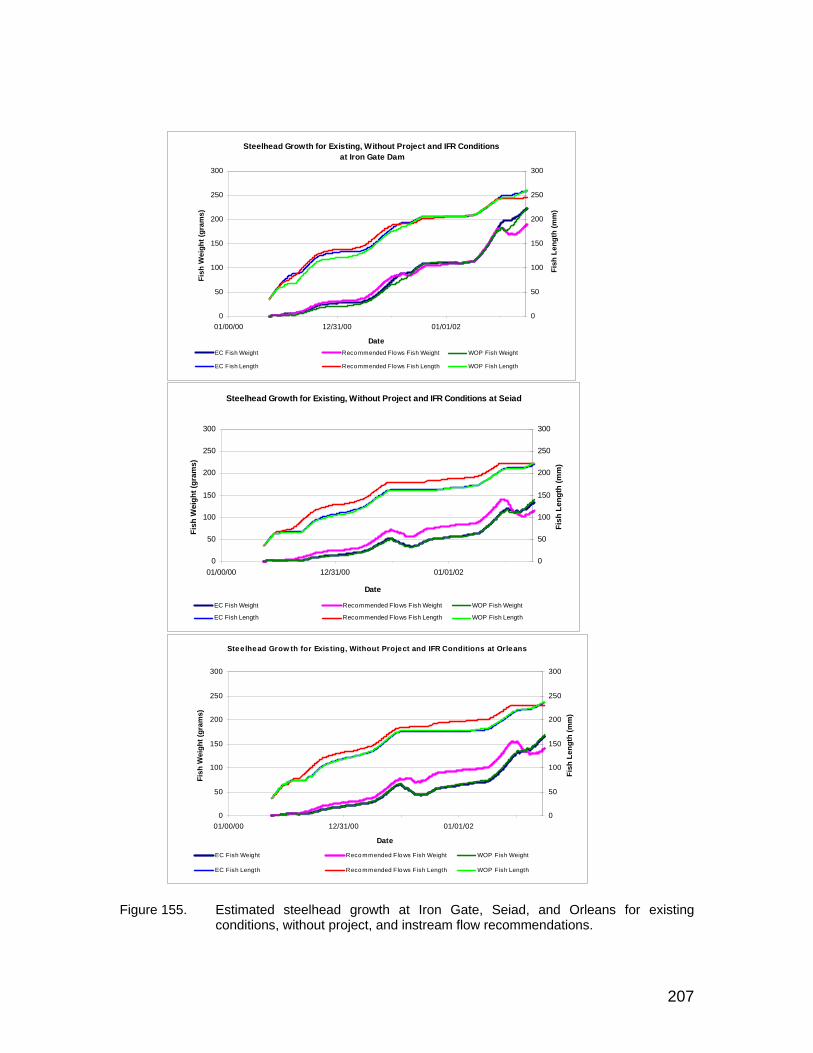
207
Figure 155. Estimated steelhead growth at Iron Gate, Seiad, and Orleans for existing
conditions, without project, and instream flow recommendations.
Steelhead Growth for Existing, Without Project and IFR Conditions at Iron Gate Dam
0
50
100
150
200
250
300
01/00/00 12/31/00 01/01/02
Date
Fish
Wei
ght (
gram
s)
0
50
100
150
200
250
300
Fish
Len
gth
(mm
)
EC Fish Weight Recommended Flows Fish Weight WOP Fish Weight
EC Fish Length Recommended Flows Fish Length WOP Fish Length
Steelhead Growth for Existing, Without Project and IFR Conditions at Seiad
0
50
100
150
200
250
300
01/00/00 12/31/00 01/01/02
Date
Fish
Wei
ght (
gram
s)
0
50
100
150
200
250
300
Fish
Len
gth
(mm
)
EC Fish Weight Recommended Flows Fish Weight WOP Fish Weight
EC Fish Length Recommended Flows Fish Length WOP Fish Length
Steelhead Grow th for Existing, Without Project and IFR Conditions at Orleans
0
50
100
150
200
250
300
01/00/00 12/31/00 01/01/02
Date
Fish
Wei
ght (
gram
s)
0
50
100
150
200
250
300
Fish
Len
gth
(mm
)
EC Fish Weight Reco mmended Flo ws Fish Weight WOP Fish Weight
EC Fish Length Reco mmended Flo ws Fish Length WOP Fish Length
208
Estimated Chinook Outmigrants using SALMOD SALMOD was utilized to estimate the annual outmigrant totals for the 1961 to 2000 water year simulation period based on existing conditions, BOR Natural Flow study, consumptive use, USGS no project, and our flow recommendations. In the simulations based on our flow recommendations, the annual exceedence for each water year was used to set the appropriate monthly instream flow targets below Iron Gate Dam using the data in Table 27. Figures156 and 157 show a comparison of the number of Chinook exiters for each scenario and clearly demonstrates that the flow recommendations provide consistently better estimated salmon production over the entire 40-year simulation period. We attribute this to the improved temperature regimes as well as increased availability of physical habitat, which are inherently incorporated into the SALMOD simulations.
Figure 156. Estimated total Chinook exiters based on application of SALMOD for each flow
scenario. We conclude from these assessments that our recommended flow regimes provide a substantial potential benefit to Chinook production within the main stem Klamath River compared to existing conditions.
Comparison of AlternativesSIAM-SALMOD Modeled Chinook Exiters, Water Years 1961- 2000
100000
600000
1100000
1600000
2100000
2600000
3100000
1961
1962
1963
1964
1965
1966
1967
1968
1969
1970
1971
1972
1973
1974
1975
1976
1977
1978
1979
1980
1981
1982
1983
1984
1985
1986
1987
1988
1989
1990
1991
1992
1993
1994
1995
1996
1997
1998
1999
2000
Date
Num
bers
of C
hino
ok F
ry a
nd S
mol
t Exi
ters
Instream Flow Recomendations, All Fry and Smolts Con All Smolts and FryBor Nat Flow, All Fry and Smolts USGS No_Proj All Fry and SmoltsUSGS Proj All Fry and Smolts
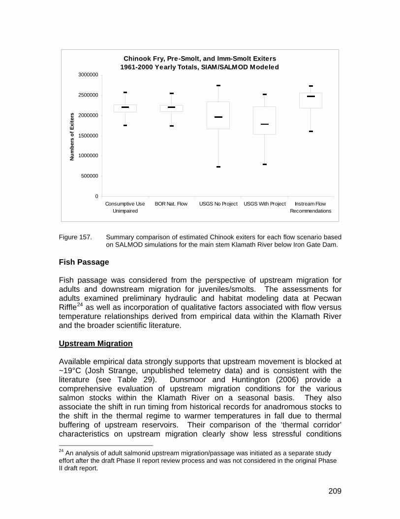
209
Figure 157. Summary comparison of estimated Chinook exiters for each flow scenario based
on SALMOD simulations for the main stem Klamath River below Iron Gate Dam. Fish Passage Fish passage was considered from the perspective of upstream migration for adults and downstream migration for juveniles/smolts. The assessments for adults examined preliminary hydraulic and habitat modeling data at Pecwan Riffle24 as well as incorporation of qualitative factors associated with flow versus temperature relationships derived from empirical data within the Klamath River and the broader scientific literature. Upstream Migration Available empirical data strongly supports that upstream movement is blocked at ~19°C (Josh Strange, unpublished telemetry data) and is consistent with the literature (see Table 29). Dunsmoor and Huntington (2006) provide a comprehensive evaluation of upstream migration conditions for the various salmon stocks within the Klamath River on a seasonal basis. They also associate the shift in run timing from historical records for anadromous stocks to the shift in the thermal regime to warmer temperatures in fall due to thermal buffering of upstream reservoirs. Their comparison of the ‘thermal corridor’ characteristics on upstream migration clearly show less stressful conditions 24 An analysis of adult salmonid upstream migration/passage was initiated as a separate study effort after the draft Phase II report review process and was not considered in the original Phase II draft report.
Chinook Fry, Pre-Smolt, and Imm-Smolt Exiters 1961-2000 Yearly Totals, SIAM/SALMOD Modeled
0
500000
1000000
1500000
2000000
2500000
3000000
Consumptive UseUnimpaired
BOR Nat. Flow USGS No Project USGS With Project Instream FlowRecommendations
Num
bers
of E
xite
rs

210
under the assumed without project scenario runs compared to existing conditions as illustrated in Figures 158 and 159 for the spring and fall periods.
Figure 158. Weekly average water temperatures within the main stem Klamath River during
the spring migration period for anadromous adults (after, Dunsmoor and Huntington 2006, used with permission).
Figure 159. Weekly average water temperatures within the main stem Klamath River during
the fall migration period for anadromous adults (after, Dunsmoor and Huntington 2006, used with permission).
Based on telemetry data for chinook migrations during 2002, 2003, and 2004, Dunsmoor and Huntington (2006) were able to demonstrate a clear relationship between movement timing and changes in thermal conditions as illustrated in Figure 160.

211
Figure 160. Contour plot of thermal conditions within the main stem Klamath River during
2002, 2003, and 2004 for steelhead and adult salmon showing the run timing of Chinook returning to Iron Gate Hatchery (after Dunsmoor and Huntington 2006, used with permission).
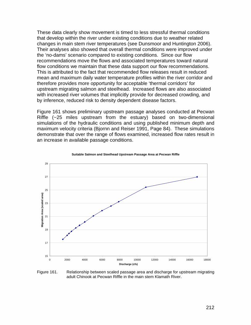
212
These data clearly show movement is timed to less stressful thermal conditions that develop within the river under existing conditions due to weather related changes in main stem river temperatures (see Dunsmoor and Huntington 2006). Their analyses also showed that overall thermal conditions were improved under the ‘no-dams’ scenario compared to existing conditions. Since our flow recommendations move the flows and associated temperatures toward natural flow conditions we maintain that these data support our flow recommendations. This is attributed to the fact that recommended flow releases result in reduced mean and maximum daily water temperature profiles within the river corridor and therefore provides more opportunity for acceptable ‘thermal corridors’ for upstream migrating salmon and steelhead. Increased flows are also associated with increased river volumes that implicitly provide for decreased crowding, and by inference, reduced risk to density dependent disease factors. Figure 161 shows preliminary upstream passage analyses conducted at Pecwan Riffle (~25 miles upstream from the estuary) based on two-dimensional simulations of the hydraulic conditions and using published minimum depth and maximum velocity criteria (Bjornn and Reiser 1991, Page 84). These simulations demonstrate that over the range of flows examined, increased flow rates result in an increase in available passage conditions.
Suitable Salmon and Steelhead Upstream Passage Area at Pecwan Riffle
15
17
19
21
23
25
27
29
0 2000 4000 6000 8000 10000 12000 14000 16000 18000
Discharge (cfs)
Mig
ratio
n A
rea
(sca
led
area
)
Figure 161. Relationship between scaled passage area and discharge for upstream migrating
adult Chinook at Pecwan Riffle in the main stem Klamath River.

213
Outmigration Dunsmoor and Huntington (2006) and Deas and Orlob (2000) demonstrated that under most flow conditions, the zone of high thermal stress below Iron Gate Dam extends downstream below about Seiad Valley, after which, the cumulative accretions ameliorate extreme water temperatures. The exception to this occurs under extremely low flows, when releases from Iron Gate Dam can make up over 30 percent of the flow at the estuary and stressful thermal conditions can extend farther downstream. Collection data from the main stem indicates that Chinook outmigrate from this reach from mid-May through about mid-June and appear to move when they reach approximately 55mm and/or when water temperatures begin to approach ~20°C. Analyses presented on fish growth above, support these findings that show this size range is achieved typically by mid-May to mid-June depending on the specific thermal regime for a given year. We note that our flow recommendations, which have higher flows during this period, result not only in more bioenergetically favorable conditions for growth, but also result in decreased travel times compared to existing conditions (see Figure 162). In Figure 162, we have shown the location of larger tributaries between Iron Gate Dam and Seiad Valley. This provides the benefit of moving fish quicker through the high thermal stress zone above Seiad Valley. The decreased travel time also results in a higher probability of encountering thermal refugia per unit time during downstream migrations, which we maintain is a net benefit through risk reduction associated with prolonged exposure to main stem water temperatures in excess of 22°C.
Figure 162. Relationship between discharge and travel time in the main stem Klamath River
below Iron Gate Dam to approximately Seiad Valley. Solid lines mark locations of thermal refugia associated with creek inflows. (Travel times computed from Deas and Orlob (1999), used with permission).
Travel Time versus Discharge
0.0
10.0
20.0
30.0
40.0
50.0
60.0
600 800 1000 1200 1400 1600
Flow (cfs)
Trav
el T
ime
(hrs
)
Bogus Willow Cottonwood Shasta Humbug Beaver Horse Scott Walker

214
Fish Disease Subsequent to the review process of the draft report, extensive fish die-offs have been recorded within the main stem Klamath River (CDFG 2004, USFWS 2002a/b, NRC 2004). Contributing factors have been associated with high water temperatures, low flows, and moderately high salmonids densities. It is beyond the scope of this report to undertake quantitative assessments associated with fish disease; however, we note that our recommendations generally result in increased flow during the critical summer period compared to existing conditions. We believe this has the potential to reduce the ecological risk to disease factors by providing more river volume that reduces crowding, which in turn reduces exposure risk to infection. The higher flow rates also result in lower water temperatures, which reduce the incubation times associated with identified disease organisms. Increased flows also result in higher velocities that potentially reduce ‘dead zone’ areas within the channel favored by free-swimming stages and intermediate hosts (e.g., polychaete worms). Ramping Rates We reviewed the proposed ramping rates as part of PacifiCorp relicensing application that specify a ramp rate of 50 cfs per 2-hour period at Iron Gate Dam when flows are within the hydraulic capacity of the hydropower plant. Recommended ramping rates also limit flow reductions to 150 cfs per day. We concur with these recommend rates and defer to the outcome of the FERC process in this regard. Potential Upstream Consequences on Klamath Project Operations SIAM was initially utilized to assess the implications of our flow recommendations on Upper Klamath Lake elevations and related deliveries to various demand areas. However, instabilities in the carry-over reservoir volumes between each simulated water year using our exceedence based flow recommendations were observed. These dramatic changes in reservoir storage volumes cast doubt on the efficacy of these simulations for comparative purposes and so were discarded. We did however verify that our recommended flow targets were released below Iron Gate Dam and similar magnitudes of simulated river temperatures between SIAM and RMA 2/11 results were obtained for the 2000 to 2003 period. We are in the process of using the RMA 2/11 models to evaluate flow recommendations associated with several dam removal options that will include comparative evaluations of existing conditions and our existing flow recommendations. It is anticipated that some increased shortages to out-of-stream uses will occur associated with the increased flow regimes during the late summer compared to existing operations, but the extent and magnitude are unknown at this time.

215
We remind the reader, that our flow recommendations are made based on the ecological needs of the Lower Klamath River and anadromous fish in particular. Our study was not commissioned to undertake any ‘optimization’ or flow balancing to meet competing water demands. The recommendations provide a frame of reference to support decision making within the policy arena, where trade-off’s between downstream flow needs versus beneficial out-of-stream uses upstream, including Upper Klamath Lake elevations necessary to protect and recover the endangered Klamath sucker will likely be debated. We also stress that the recommended flow regimes specifically address needs within the main stem Klamath River below Iron Gate Dam for all anadromous species and have not targeted our flow recommendations in the main stem for coho. As stated previously, we believe that ultimate recovery success for coho will be contingent on rehabilitation of tributary systems, which will inherently benefit main stem conditions for all anadromous species.
Conclusions Instream flow recommendations were developed for specific annual exceedence levels in terms of the corresponding target monthly flows to meet anadromous species flow needs in the main stem Klamath River. The approach relied on the Natural Flow Paradigm to select flows that closely mimic the natural flow pattern seasonally for different types of water years and directly integrates physical habitat needs. These results were integrated with temperature simulations to demonstrate that the recommendations provide equal or improved growth rates (size and weight) from Iron Gate Dam downstream to Orleans for Chinook and steelhead rearing. The growth modeling results suggest that fish should emigrate from the upper main stem beginning in mid-May to mid-June based on size and/or the point at which the simulations show no growth and is supported by outmigration timing observed for the main stem Klamath River. We provide evidence that the increased flows, which reduce maximum daily and mean daily temperatures, while increasing minimum daily temperatures provide a net bioenergetic benefit based on the equivalent ‘fish mean daily temperature’. Simulations of Chinook exiters from the system using SALMOD shows increased production potential for basically every year compared to existing conditions. Analyses were also presented that demonstrate the proposed flow regimes benefit all life stages of anadromous species during all periods of the year including upstream migration, spawning, rearing, upstream passage, and out migration compared to existing conditions. We use empirical fish observation data to document continuous use of the main stem Klamath River by anadromous species through every month of the year and relate behavioral thermoregulation associated with main stem river temperatures of ~ 22°C. Empirical data demonstrate main stem use by anadromous species at temperature up to approximately 26°C and we provide supporting evidence from the thermal preference, tolerance, and critical thermal maximum literature that

216
Chinook and steelhead can tolerate transient exposures to these water temperatures up to ~ 26°C based on physiological mechanisms associated with variable ‘acclimation’ temperatures reflective of real world river conditions. Avoidance of the main stem by coho starting in late June is consistent with their somewhat lower thermal lability. The recommended flow regime is also anticipated to reduce disease related risk factors by increasing flow volumes and likely reduce ‘slack water’ areas important to known disease organisms in the main stem river. Our analyses and results also support improved benefits with increased travel times below Iron Gate Dam that moves fish out of the highest thermal stress area associated with Seiad Valley. We believe that our analyses in support of our flow recommendations meet the ecological objectives for the flow dependent needs of the anadromous species and life stages in the main stem Klamath River (see Table 16). Recommended flow regimes during the summer periods during low flow years are not anticipated to impact existing thermal refugia based on field observations and detailed hydraulic modeling of representative sites from the main stem river. Although our recommendations provide for improved conditions within the main stem Klamath River, we maintain that the importance of protecting and/or restoring flow and temperature conditions in tributary systems is critical for long-term recovery of the anadromous stocks in the Lower Klamath Basin.
Literature Cited Aadland, L.P. (1993). Stream habitat types: their fish assemblages and
relationship to flow. North American Journal of Fisheries Management 13:790-806.
Abney, R.M. (1964). A comparative study of the past and present condition of Tule Lake. USDI Bureau of Sport Fisheries and Wildlife, Tulelake.
Acreman, M.C., M.J. Dunbar, J. Hannaford, O.M. Bragg, A.R. Black, and J.S. Rowan. (2006). Development of environmental standards (water resources). Stage 3: environmental standards. Project WFD48.
Addley, R.C., B. Bradford, and J. Ludlow (2005). Klamath River Bioenergetics Report. Institute for Natural Systems Engineering, Utah Water Research Laboratory, Utah State University, Logan, Utah. 135pp.
Addley, R.C. (2006). A mechanistic daily net energy intake approach to modeling habitat and growth of drift-feeding salmonids (particularly the genus Oncorhynchus). Ph.D. Dissertation, Department of Civil and Environmental Engineering, Utah State University, Logan, Utah.
AEIDC (1981). Arctic Environmental Information and Data Center. An assessment of environmental effects of construction and operation of the proposed Terror Lake Hydroelectric Facility, Kokiak, Alaska. Instream Flow Studies. Final Report. University of Alaska, Anchorage, AK: 418 pp.
Allan, D. (1995). Stream Ecology. Chapman and Hall, Oxford London. 387pp.

217
Annear, T., I. Chisholm, H. Beecher, A. Locke, and 12 other authors. (2002). Instream flows for riverine resource stewardship. Instream Flow Council, Cheyenne, WY. 411pp.
Annear, T., I. Chisholm, H. Beecher, A. Locke, and 12 other authors. (2004). Instream flows for riverine resource stewardship, revised edition. Instream Flow Council, Cheyenne, WY. 267pp.
Arcement, Jr., G.J. and V.R. Schneider. (1989). Guide for Selecting Manning’s Roughness Coefficients for Natural Channels and Flood Plains. United States Geological Survey Water-Supply Paper 2339. 38pp.
Arthington, A.H. and R. Lloyd (eds). (1998). Logan River trial of the Building Block Methodology for assessing environmental flow requirements. Workshop Report. Centre for Catchment and In-stream Research and Department Natural Resources, Brisbane, Australia. 85 pp.
Arthington, A.H. and G.C. Long (eds). (1997). Logan River trial of the Building Block Methodology for assessing environmental flow requirements. Background Papers. Centre for Catchment and In-Stream Research, Griffith University and Queensland Department of Natural Resource. Brisbane, Australia. 332 pp
Ayres Associates. (1999). Geomorphic and Sediment Evaluation of the Klamath River, California, below Iron Gate Dam. Report to U.S. Fish and Wildlife Service by Ayres Associates, Fort Collins, Colorado.
Bain, M.B. (1995). Habitat at the local scale: multivariate patterns for stream fishes. Bulletin Francais de la Peche et Piscic et de la Pisciculture 337/338/339:165-177.
Bain, M.B., J. T. Finn, and H. E. Booke. (1988). Streamflow regulation and fish community structure. Ecology 69(2):382-392.
Balance Hydrologics, INC. (1996). Initial assessment of pre- and post-Klamath Project hydrology on the Klamath River and Impacts of the project on instream flows and fisheries habitat. 39pp and appendix.
Bartholow, J.M. (1995). Review and Analysis of Klamath River Basin Water Temperatures as a Factor in the Decline of Anadromous Salmonids with Recommendations for Mitigation. In: Compilation of Phase I Reports for the Klamath River Basin, May 1995, River Systems Management Section, NBS-MidContinent Ecological Science Center, Fort Collins, Colorado.
Bartholow, J.M. (2005). Recent Water Temperature Trends in the Lower Klamath River, California. North American Journal of Fisheries Management 25:152–162.
Bartholow, J. M., J. Heasley, R. B. Hanna, J. Sandelin, M. Flug, S. Campbell, J. Henriksen, and A. Douglas. (2003). Evaluating water management strategies with the Systems Impact Assessment Model: SIAM, version 3. U.S. Geological Survey, Fort Collins Science Center, Open File Report 03-82, Fort Collins, Colorado. Available: http://www.fort.usgs.gov. (March 2003.)
Bartholow, J.M., S.G. Campbell, and M. Flug. (2005). Environmental assessment: Predicting the thermal effects of dam removal on the Klamath River. Environmental Management Vol. 34, No. 6, pp.856-874.
218
Beacham, T.D. and C.B. Murray. (1990). Temperature, egg size, and development of embryos and alevins of five species of pacific salmon: A comparative analysis. Transactions of the American Fisheries Society 119:927-945.
Beak Consultants, Inc. (1985). Sandy River instream flow study for the city of Portland. Beak Consultants, Ind., Portland, OR. 67 pp.
Belchik, M. (1997). Summer locations and salmonids use of cool water areas in the Klamath River: Iron Gate Dam to Seiad Creek, 1996. Yurok Tribal Fisheries Program. 18pp.
Belchik, M. (2003). Use of thermal refugia areas on the Klamath River by juvenile salmonids; Summer 1998. Yurok Tribal Fisheries Program. 36pp.
Bhosle, M.C. (2004). Estimating uncertainty in fish habitat modeling using two-dimensional hydraulics. M.S. Thesis. Utah State University. 107pp.
Bisson, P. A., J. L. Nielsen, and J. W. Ward. (1988). Summer production of coho salmon stocked in Mount St. Helens streams 3-6 years after the 1980 eruption. Transactions of the American Fisheries Society 117:322-335.
Bjornn, T.C. and D.W. Reiser. (1991). Habitat Requirements of Salmonids in Streams. In: Meehan, W.R., ed. Influences of Forest and Rangeland Management onSalmonid Fishes and Their Habitats. American Fisheries Society Special Publication. 19(4):83-138.
BOR (1954). Upper Klamath River Basin Oregon-California, A comprehensive Departmental report on the development of water related resources. United States Department of the Interior Bureau of Reclamation.
Bovee, K.D. (1986). Development and evaluation of habitat suitability criteria for use in the Instream Flow Incremental Methodology. Instream Flow Information Paper 21. U.S. Fish and Wildl. Serv. Biol. Rep. (86(7). 235pp.
Bovee, K.D., T.J. Newcomb, and T.G. Coon. (1994). Relations between habitat variability and population dynamics of bass in the Huron River, Michigan. National Biological Survey Biological Report 21. 63 pp.
Bovee, K. D. (editor) (1995). A comprehensive overview of the Instream Flow Incremental Methodology. National Biological Service, Fort Collins, Colorado. 335 pp.
Bowen, Z.H., M.C. Freeman, and K.D. Bovee. (1998). Evaluation of generalized habitat criteria for assessing impacts of altered flow regimes on warmwater fishes. Transactions of the American Fisheries Society 127:455-468.
Boydston, L.B., (1977). Adult harvest and escapement study – lower Klamath River tagging study. Performance Report, Calif. Dept. of Fish and Game.
Bozek, M.A., and F.J. Rahel. (1992). Generality of microhabitat suitability models for young Colorado River cutthroat trout (Oncorhynchus clarki pleuriticus) across sites and among years in Wyoming Streams. Canadian Journal of Fisheries and Aquatic Sciences 49:552-564.
Brett, J. R., W. C. Clarke, and J. E. Shelbourn. (1982). Experiments on thermal requirements for growth and food conversion efficiency of juvenile

219
Chinook salmon Oncorhynchus tshawytscha. Canada Fisheries and Marine Service Technical Report 1127.
Brizga, S.O. and A.H. Arthington. (2001). Guidelines for the environmental flow management in Queensland rivers, NR&M, Queensland.
Brown, L.R., and P.B. Moyle. (1991). Status of coho salmon in California. Report to the National Marine Fisheries Service, Submitted July 1991. 114pp.
Buer, K. (1981). Klamath and Shasta Rivers Spawning Gravel Study. California Department of Water Resources, Northern District.
Busby, P. J., T. C. Wainwright, and R.S. Waples. (1994). Status review for Klamath Mountains Province steelhead. U.S. Dep. Commer., NOAA Tech. Memo. NMFS-NWFSC-19, 130pp.
Bustard, D.R. and D. W. Narver. (1975). Aspects of the winter ecology of juvenile coho Salmon (Oncorhynchus kisutch) and steelhead trout (Salmo gairdneri). J. Fish. Res. Board Can. 32:667-680.
CDFG (1959). The Anadromous Fisheries of the Klamath River with Respect to the Iron Gate Development, Department of Fish and Game.
CDFG. (1995). Klamath River Basin Fall Chinook Salmon Run-Size, In-River Harvest Escapement – 1995 Season. Klamath Trinity Program.
CDFG (2004). September 2002 Klamath River Fish-Kill: Final Analysis of Contributing Factors and Impacts. 173pp.
CDM (1986). Minimum Instream Flow Study. Camp, Dresser, and McKee. Final Report. Commonwealth of Virginia State Water Control Board.
CH2MHill. (1985). Klamath River Basin Fisheries Resource Plan. Contract Report to US. Bureau of the Interior, Bureau of Indian Affairs. CH2M-Hill, Redding, Calif. 404pp.
Chow, V.T. (1959) Open-Channel Hydraulics. McGraw-Hill Book Company. ISBN 07-010776-9. 680pp.
Coots, M. (1954). Klamath River 1953 King Salmon Count Klamathon Racks, Siskiyou, Inland Fisheries Branch California Department of Fish and Game.
Coots, M. (1962). Shasta River, Siskiyou County, 1958 king salmon count with yearly totals from 1930-1961. California Department of Fish and Game. Inland fisheries Branch. Marine Resources Administrative Report No. 62-64. 5 p.
Coots, M. (1967). Anglers guide to the Klamath River. Calif. Dept. of Fish and Game, Sacramento, California.
Coots, M. (1972). Fish and wildlife resource relationships in Basin 1A-Klamath River. California Department of Fish and Game, Task 3.
Coots, M. (1973). A study of juvenile steelhead, Salmo gairdenerii gairdernii Richardson, in San Gregorio Creek and lagoon, San Mateo County, March through August, 1971. CDFG Anad. Fish. Br. Admin.
COST (European Cooperation in the field of Scientific and Technical Research). (2005). COST 626: European Aquatic Modelling Network: Proceedings from the final meeting in Silkeborg, Denmark, May 2005. National Environmental Research Institute. 397pp.
220
Cox, D. K., and C. C. Coutant. (1981). Growth dynamics of juvenile striped bass as functions of temperature and ration. Transactions of the American Fisheries Society 110: 226–238.
Deas, M.L., and G.T. Orlob (1999). Klamath River Modeling Project. Center for Environmental and Water Resources Engineering, Department of Civil and Environmental Engineering, Water Resources Modeling Group. U.C. Davis. Project No. 96-HP-01. 236pp.
Deas, M.L., S.K. Tanaka, and J.C. Vaughn. (2006). Klamath River thermal refugia study: Flow and temperature characterization – Final Report. Watercourse Engineering, Inc. March 6, 2006. 244pp.
Dunbar, M., and A. Ibbotson. (2001). Further validation of PHABSIM for the habitat requirements of salmonid fish. Centre for Ecology and Hydrology Final Project Report to the Environment Agency (W6-036) and CEH (C00962).
Dunbar, M., A. Gustard, M.C. Acreman, and C.R.N. Elliott. (1998). Overseas approaches to setting river flow objectives. R&D Technical Report W6B(96)4. 83pp.
Dunsmoor L.K. and C.W. Huntington. (2006). Suitability of environmental conditions within Upper Klamath Lake and the migratory corridor downstream for use by anadromous salmonids. Technical memorandum to the Klamath Tribes. March 2006. 147pp.
Elliott, J.M. (1975). The growth rate of brown trout (Salmo trutta L.) fed on maximum rations. J. Anim. Ecol. 44:805-821.
EPRI (1986). Instream Flow Methodologies. Final Report, EA-4819 Research Project 2194-2. Electric Power Research Institute, Palo Alto, California.
Everest, F.H., and D.W. Chapman. (1972). Habitat selection and spatial interaction by juvenile Chinook salmon and steelhead trout in two Idaho streams. J. Fish. Res. Bd. Canada 29:91-100.
Flint, A.L. and L.E. Flint. (2006). Estimation of hourly stream temperatures in unmeasured tributaries to the Lower Klamath River, California. USGS. 42pp.
Flug, M., and J. F. Scott. (1998). Modeling and Management of Water in the Klamath River Basin: Overcoming Politics and Conflicts. In: ASCE 1998 International Water Resources Engineering Conference Proceedings, "Water Resources Engineering 98", Abt, S.R., et. al., (Editors), American Survey of Civil Engineers, VA, Vol. 1, 938-943.
Fortune, J.D., A.R. Gerlach, and C.J. Hanel. (1966). A study to determine the feasibility of establishing salmon and steelhead in the Upper Klamath Basin. Oregon State Game Commission and Pacific Power and Light.
From, J. and G. Rasmussen. (1984). A growth model, gastric evacuation, and body composition in rainbow trout, Salmo gairdneri Richardson, 1836. Dana, 3:61-139.
Garret, R. (1997). Klamath/Central Pacific Coast Ecoregion Restoration Strategy, Vols. I-IV, Klamath Falls, OR, Klamath Basin Ecosystem Restoration Office.

221
Giannico, G.R. (2000). Habitat selection by juvenile coho salmon in response to food and woody debris manipulations in suburban and rural stream sections. Can. J. Fish. Aquat. Sci. 57: 1804–1813.
Gore, J.A. (1989). Models for predicting benthic macroinvertebrate habitat suitability under regulated flows. In: J.A. Gore, J.A. and G.E. Petts, (eds.), Alternatives in regulated river management, Pp. 254-265, CRC Press Inc., Boca Raton, Florida.
Gore, J.A., and J.M. Nestler. (1988). Instream flow studies in perspective. Regulated Rivers: Research and Management. Vol. 2:93-101.
Gorman, O. T., J. R. Karr. (1978). Habitat structure and stream fish communities. Ecology. 59(3):507-515.
Hamilton, J.B., G.L. Curtis, S.M. Snedaker, and D.K. While. (2005). Distribution of Anadromous Fishes in the Upper Klamath River Watershed Prior to Hydropower Dams - A Synthesis of the Historical Evidence. Fisheries. Vol. 30. No. 4. pp. 10-20.
Hampton, M. (1988). Development of habitat preference criteria for anadromous salmonids of the Trinity River. U.S. Dept. Int., Fish Wildlife Serv., Div. Ecol. Serv., Sacramento, California. 93 pp.
Hanna, R.B., and S.G. Campbell. (2000). Water Quality Modeling in the Systems Impact Assessment Model for the Klamath Basin - Keno, Oregon to Seiad Valley, California. U.S. Geological Survey Open File Report 99-113. 84 pp.
Hanson, P.C., Johnson, T.B., Schindler, D. E., and Kitchell, J. F. (1997). Fish bioenergetics 3.0 for Windows. University of Wisconsin Sea Grant Institute, Madison.
Harby, A., M. Baptist, M. J. Dunbar, and S. Schmutz (editors). (2004). State-of-the-art in data sampling, modelling analysis and applications of river habitat modeling. COST Action 626 Report. 313pp.
Hardin, T.S., R.T. Gross, M.B. Ward, and G.E. Smith. (2005). Habitat Suitability Criteria for Anadromous Salmonids in the Klamath River, Iron Gate Dam to Scott River, California. An investigation for the U.S. Fish and Wildlife Service and California Department of Fish and Game. California Department of Fish and Game Stream Evaluation Report 05-1, March 2005. 73pp.
Hardy, T.B. (1998). The Future of Habitat Modeling and Instream Flow Assessment Techniques. Regulated Rivers: Research and Management 14:405-420.
Hardy, T.B. (1999). Evaluation of Interim Instream Flow Needs in the Klamath River – Phase I. Institute for Natural Systems Engineering, Utah Water Research Laboratory, Utah State University. 53pp +Appendicies.
Hardy, T.B. (2000). The Theory and Application of the Physical Habitat Simulation System (PHABSIM) for Windows (PHABWin-98) Lecture and Laboratory Manual. Institute for Natural Systems Engineering, Utah State University. 273pp.
Harper, D.M. and J.D. Ferguson (Eds.). (1995). The Ecological Basis for River Management. West Sussex, England: John Wiley & Sons Ltd. 614pp.
222
Hassler, T.J. (1987). Species profiles: Life histories and environmental requirements of coastal fishes and invertebrates (Pacific Southwest)--coho salmon. U.S. Fish and Wildl. Serv. Biol. Rep. 82(11.70). 19 pages.
Heggenes, J. (1990). Habitat utilization and preferences in juvenile Atlantic salmon (Salmo salar) in streams. Pages 342-354 John Wiley and Sons.
Heifetz, J., M.L. Murphy, and K.V. Koski. (1986). Effects of logging on winter habitat of juvenile salmonids in Alaskan streams. N. Am. J. Fish. Manage. 6:52-58.
Hill, M.R., W.S. Platts, and R.L. Beschta. (1991). Ecological and geomorphological concepts for instream and out-of-channel flow requirements. Rivers 2:198-210.
Hiser, C. (1994). CDFG, Iron Gate Hatchery. Hokanson, K.E.F., Kleiner, C.F., and Thorslund, T.W. (1977). Effects of
constant temperatures and diel temperature fluctuations on specific growth and mortality rates and yield of juvenile rainbow trout, Salmo gairdneri. J. Fish. Res. Bd. Can. 34:639-648.
Horwitz, R.J. (1978). Temporal variability patterns and the distributional patterns of stream fishes. Ecological Monographs, Vol. 48: 307-321.
Hosey, and Associates. (1986). Unpublished curves (curve lib). Huff, D.D., S.L. Hubler, and A.N. Borisenko. (2005). Using field data to estimate
the realized thermal niche of aquatic vertebrates. North American Journal of Fisheries Management 25:346-360.
Hutchinson, G.E. (1957). Concluding Remarks. Cold Spring Harbor Symposium, Quant. Biol., 22, 415-427.
Jager, H.I., D.L. Deangelis, M.J. Sale, W. Van Winkle, D.D. Schmoyer, M.J. Sabo, D.J. Orth, and J.A. Lukas. (1993). An individual-based model for smallmouth bass reproduction and young-of-the-year dynamics in streams. Rivers 4:91-113.
Jowett, I.G. (1992). Models of the abundance of large brown trout in New Zealand rivers. North American Journal of Fisheries Management 12:417-432.
Jowett, I.G., J. Richardson, J.F. Biggs, C.W. Hickey, and J.M. Quinn. (1991). Microhabitat preferences of benthic invertebrates and the development of generalized Deleatidium spp. Habitat suitability curves, applied to four New Zealand streams. New Zealand Journal of Marine and Freshwater Research 25:187-199.
KRBFTF. (1991). Long Range Plan for the Klamath River Basin Conservation Area Fishery Restoration Program. Yreka, CA, Klamath River Basin Fisheries Task Force.
Kirby, C. and W.R. White (Eds.). (1994). Integrated River Basin Development. Presentations at the International conference on integrated river basin development, sponsored by HR Wallingford and Institute of Hydrology, Wallingford, UK, September 1994. West Sussex, England: John Wiley & Sons Ltd. 537pp.
Labadie, J.W. (1988). Program MODSIM: River basin network flow model for the microcomputer. Department of Civil Engineering, Colorado State
223
University, Ft. Collins, Colorado. Download and documentation available on website at http://modsim.engr.colostate.edu/.
Larson, Z., Belchik, M. (1998). A preliminary status review of eulachon and Pacific lamprey in the Klamath River Basin. Yurok Tribal Fisheries Program Technical Report. 13pp.
Leidy R.A., and G.R. Leidy. (1984). Life stage periodicities of anadromous salmonids in the Klamath River basin, northwestern California. U.S. Fish and Wildlife Service, Sacramento, Calif. 21pp plus tables and appendices.
LaRue, E.C. (1922). Klamath River and its Utilization. Office of State Engineer, Salem, Oregon. 153 pp.
Lee, R. M., J. N. Rinne. (1980). Critical thermal maxima of five trout species in the southwestern United States. Transactions of the American Fisheries Society.109:632-635.
Lobb, M. D. III and D. J. Orth. (1991). Habitat use by an assemblage of fish in a large warmwater stream. Transactions of the American Fisheries Society 120:65-78.
McBain and Trush. (1995). River Channel Morphological and Sediment Changes in the Klamath Basin, Oregon and California: Summary of Available Geomorphic Data, Data Deficiencies, and Identification of Critical Geomorphic Issues. Report to the Technical Working Group, Klamath River Fisheries Task Force, by McBain and Trush, Arcata, California.
McCullough, D.A. (1999). A review and synthesis of effects of alterations to the water temperature regime on freshwater life stages of slamoninds, with special reference to Chinook salmon. Contract report EPA 910-R-99-010, July 1999.
McLean, S.R., S.R. Wolfe, and J.M. Nelson. (1999). Predicting boundry shear stress and sediment transport over bed forms. Journal of Hydraulic Engineering. July 1999:725-736.
Modde, T. and T. B. Hardy. (1992). Influence of Different Microhabitat Criteria on Salmonid Habitat Simulation. Rivers: 3:1 37-44 pp.
Moffett, J.W. and S.H. Smith. (1950). Biological investigations of the fishery resources of the Trinity River, California. Special Scientific Report No. 12. U.S. Fish and Wildlife Service. 71pp.
Moore, K.M.S. and S.V. Gregory (1988). Summer Habitat Utilization and Ecology of Cutthroat Trout Fry (Salmo Clarki) in Casdace Maountain Streams. Can. J. Fish. Aquat. Sci.; 45(11):1921-1930.
Moyle, P.B. (1976). Inland Fishes of California. University of California Press. Berkley and Los Angeles. 404pp.
Moyle, P.B., J.E. Williams, and E.D. Wikramanayake. (1989). Fish species of special concern of California. Final report to California Dept. of Fish and Game, Contract No. 7337.
Moyle, P.B., and D.M. Baltz. (1985). Microhabitat use by an assemblage of California stream fishes: Developing criteria for instream flow determinations. Transactions of the American Fisheries Society 114:695-704.

224
Myrick, C. A. and J. J. Cech. (2001). Temperature effects on Chinook steelhead: a review focusing on California’s Central Valley Available: <http://www.cwemf.org/Pubs/Tempreview.pdf>.
Nehring, R.B. and R.M. Anderson. (1993). Determination of population-limiting critical salmonid habitats in Colorado streams using IFIM/PHABSIM. Rivers 4:1-19.
NMFS (1997). Endangered and Threatened Species; Threatened Status for Southern Oregon/Northern California Coast Evolutionarily Significant Unit (ESU) of Coho Salmon. Final Rule; notice of determination. 62 FR 87.
NMFS (1998). Endangered and Threatened Species: Threatened Status for Two ESUs of Steelhead in Washington, Oregon, and California. Final rule; notice of determination. 63 FR 13347.
NRC (1996). National Research Council. Upstream: Salmon and Society in the Pacific Northwest. Washington, D.C.: National Academy Press. 452pp.
NRC (2004). National Research Council. Endangered and threatened fishes in the Klamath River Basin – Causes of decline and strategies for recovery. Washington, D.C.: National Academy Press. 397pp.
NRC (2005). National Research Council. The science of instream flows – A review of the Texas Instream Flow Program. Washington, D.C.: National Academy Press. 149pp.
Nelson, J.M. (1996). Predictive techniques for river channel evolution and maintenance. Air and Soil Pollution. 90:321-333.
Nelson, J.M., R.L. Shreve, R. McLean, and T.G. Drake. (1995). Role of near-bed turbulence structure in bed load transport and bed form mechanics. Water Resources Research. 31(8):2071-2086.
NCRWQB (2006). North Coast Regional Water Quality Control Board. RMA-2 and RMA-11 flow and water quality modeling results for natural flows and existing conditions within the Klamath River for TMDL assessments.
Olden, J.D. and N.L. Poff. (2003). Redundancy and choice of hydrologic indices for characterizing streamflow regimes. River Res. Applic. 19:101-121.
Orth D.J., (1987). Ecological considerations in the development and application of instream flow-habitat models. Regulated Rivers: Research and Management. Vol. 1, 171-181.
Orth, D.J. and O.E. Maughan. (1982). Evaluation of the incremental methodology for recommending instream flows for fish. Transactions of the American Fisheries Society 111:413-445.
PacifiCorp (2004). FINAL TECHNICAL REPORT - Klamath Hydroelectric Project (FERC Project No. 2082) Water Resources.
PacifiCorp (2006). Cumulative filings under the FERC relicensing process. Perry, T., A. Leib, A. Harrison, M. Spears, T. Mull, E. Cohen, J. Rasmussen, and
J. Hicks. (2005). Natural flow of the Upper Klamath River – Phase I. Natural inflow to, natural losses from, and natural outfall of Upper Klamath Lake to the Link River and the Klamath River at Keno. USDOI, Bureau of Reclamation. 115pp. + appendices.

225
Petts, G. and P. Calow (Eds.). (1996). River Restoration: Selected extracts from the rivers handbook edited by P. Calow and G. Petts. Cambridge, MA: Blackwell Science Ltd. 231pp.
PFMC (1991). Preseason Report I, Stock Abundance Analysis for 1991 Ocean Salmon Fisheries. Prepared by the Salmon Technical Team for the Pacific Fishery Management Council, Portland Oregon.
PFMC (1998). Preseason Report I, Stock Abundance Analysis for 1999 Ocean Salmon Fisheries. Prepared by the Salmon Technical Team for the Pacific Fishery Management Council, Portland Oregon.
Poff, N.L., J.D. Allan, M.B. Bain, J.R. Karr, K.L. Prestegaard, B.D. Richter, R.E. Sparks, and J.C. Stromberg. (1997). The natural flow regime – A paradigm for river conservation and restoration.
Postel, S. and B. Richter. (2003). Rivers for life. Washington, D.C.: Island Press. 253pp.
Powers, M.E.. Matthews, W.J., and Stewart, A.J. (1985). Grazing minnows, piscivorous bass, and stream algae: Dynamics of a strong interaction. Ecology 66(5): 1448-1456.
PWA (2002). Hydrodynamic modeling of Upper Klamath Lake. Phillip Williams and Associates, Ltd. November 11, 2002. Technical report prepared for the Bureau of Reclamation. 17pp.
Railsback, S.F., R.F. Blackett, and N. D. Pottinger. (1993). Evaluation of the fisheries impact assessment and monitoring program for the Terror Lake hydroelectric project. Rivers 4(4):312-327.
Rankel, G.L. (1982). An appraisal of the status and future of wild Chinook salmon in the Klamath River drainage. Wild Trout and Steelhead Fisheries: Laws and Law Enforcement. Proceedings of a Symposium. California Trout.
Reiser, D.W., T.A. Wesche and C. Estes. (1989). Status of instream flow litigation and practices in North America. Fisheries 14(2):22-29.
Reiser, D.W., T. Nightengale, N. Hendrix, and S. Beck. (2005). Effects of pulse flows on benthic macroinvertebrates and fish: A review and synthesis of information. R2 Resource Consultants. April 2005. 148pp.
Risley, J.C. and S.A. Rounds. (2006). Evaluation and Review of Recent Klamath River Water-Temperature Modeling Studies. U.S. Geological Survey, Reston, Virginia. 27pp.
Sanford, R. A. (1984). PHABSIM error analyses: Techniques and case studies. M.S. Thesis.University of Washington, Seattle.
Scheidegger, K.J., and M.B. Bain. (1995). Larval fish distribution and microhabitat use in free-flowing and regulated rivers. Copeia 1:125-135.
Schlosser, I. J. (1987). The role of predation in age-and size-related habitat use by stream fishes. Ecology 68(3):651-659.
Schmidt, L.J. and J.P. Potyondy. (2004). Quantifying channel maintenance instream flows: An approach for gravel-bed streams in the western United States. U.S. Department of Agriculture, Forest Service, Rocky Mountain Research Station, General Technical Report RMRS-GTR-128. 33pp.

226
Schoener, T.W. (1988). The ecological niche. Pages 79-111 in J.M. Cherrett, eds., Ecological Concepts. Blackwell Scientific.
Schirvell, C.S. (1986). Pitfalls of physical habitat simulation in the Instream Flow Incremental Methodology. Canadian Fisheries and Aquatic Sciences Technical Report 1460. 68 pp.
Schirvell, C.S. (1994). Effect of changes in streamflow on the microhabitat use and movements of sympatic juvenile coho (Oncorhynchus kisutch) and Chinook salmon (O. tshawytscha) in a natural stream. Can. J. Fish. Aquat. Sci. 51:1644-1652.
Scott, J. F. and M. Flug. (1998). Modeling With MODSIM: Klamath River Basin Water Quantity for Protecting Fish and Other Resource Values. In: First Federal Interagency Hydrologic Modeling Conference Proceedings, Subcommittee on Hydrology of the Interagency Advisory Committee on Water Data, Las Vegas, Nevada. April 19-23, 1998; Vol 2, 8-103 - 8-110.
Shaw, T.A., C. Jackson, D Nehler, and M. Marshall. (1997). Klamath River (Iron Gate to Seiad Creek) lIfe stage periodicities for Chinook, coho, and steelhead. July 1997. U.S. Department of Interior, U.S. Fish and Wildlife Service Coastal California Fish and Wildlife Office, Arcata, California. 63pp.
Smith, J.J., and H.W. Li. (1983). Energetic factors influencing foraging tactics of juvenile steelhead trout, Salmo gairdneri. Pages 173-180 in D.L.G. Noakes, eds., Predators and prey in fishes. The Hague.
SNIFFER (2006). Development Of Environmental Standards: (Water Resources) Stage 3: Environmental Standards.
Snyder, J.O. (1930). Salmon of the Klamath River California. Fish Bulletin No. 34. Division of Fish and Game. 130pp.
Snyder, J.O. (1933). A steelhead migration in the Shasta River. Calif. Fish Game 19(4): 252-254.
Stalnaker, C., B.L. Lamb, J. Henriksen, K. Bovee, and J. Bartholow. (1995). The Instream Flow Incremental Methodology – A Primer for IFIM. U.S. Department of the Interior, National Biological Service, Washington, D.C. Biological Report 29, March 1995.
State of Queensland, Department of Natural Resources and Mines. (2001). Pioneer Valley Water Resource Plan.
Statzner, B., and B. Higler. (1986). Stream hydraulics as a major determinant of benthic invertebrate zonation patterns. Freshwater Biology 16:127-139.
Strange, J. (2006). Adult Chinook salmon migration in the Klamath River Basin: 2005 sonic telemetry study report. Yurok Tribal Fisheries Program. 5pp.
Strange, J. (2006). Ph.D. research unpublished radio tracking data and analyses for Chinook upstream migrations and temperatures. Used with permission.
Studley, T.K. and nine other authors. (1995). Response of fish populations to altered flows project. Volume 1:Predicting trout populations from stream flow and habitat variables. Pacific Gas and Electric Company, San Ramon, CA 94583. Vvpp.
227
Stutzer, G. M., J. Ogawa, N. J. Hetrick, and T. Shaw. (2006). An Initial Assessment of Radiotelemetry for Estimating Juvenile Coho Salmon Survival, Migration Behavior, and Habitat Use in Response to Iron Gate Dam Discharge on the Klamath River, California. U. S. Fish and Wildlife Service, Arcata Fish and Wildlife Office, Arcata Fisheries Technical Report Number TR2006-05, Arcata, California.
Suchanek, P. M., K. J. Kuntz, and J. P. McDonnell. (1984a). The relative abundance, distribution and instream flow relationships of juvenile salmon in the lower Susitna River. Report #7, part 2. Alaska Dept. of Fish and Game, Susitna River Aquatic Studies Program, Anchorage, Alaska.
Suchanek, P. M., R. P. Marshall, S. S. Hale, and D. C. Schmidt. (1984b). Juvenile salmon rearing suitability criteria. Part 3 in D. C. Schmidt, S. S. Hale, D. L. Crawford, and P. M. Suchanek, eds. Resident and juvenile anadromous fish investigations (May-October 1983). Alaska Dept. Fish Game Susitna Hydro Aquatic Studies Report No. 2, Anchorage, Alaska.
Sullivan, C.M. (1989). Juvenile life history and age composition of mature fall Chinook salmon returning to the Klamath River, 1984-1986. Masters thesis. Humboldt State University, Arcata, California. 134pp.
Sullivan, K., D. J. Martin, R. D. Cardwell, J. E. Toll, and S. Duke. (2000). An analysis of the effects of temperature on salmonids of the Pacific Northwest with implications for selecting criteria. Portland, OR: Sustainable Ecosystems Institute.
Tanaka, S.K., M.L. Deas, R.J. Sutton, T. Soto, and A. Corum. (2006). Physical characterization of a Klamath River thermal refugia under various hydrologic and meteorological conditions. Draft report. 33pp.
Thomas, J.A., and K.D. Bovee. (1993). Application and testing of a procedure to evaluate transferability of habitat suitability criteria. Regulated Rivers: Research and Management 8:285-294.
Thompson, D.M., J.M. Nelson, and E.E. Wohl. (1998). Interactions between pool geometry and hydraulics. Water Resources Research. 34(12):3673-3681.
Topping, D.J., D.M. Rubin, J.M. Nelson, P.J. Kinzel III, I.C. Corson. (2000). Colorado River sediment transport. 2. Systematic bed-elevation and grain-size effects of sand supply limitation. Water Resources Research. 36(2):543-570.
USBR (1997). Biological Assessment of the Klamath Project 1997 Operations Plan.
USACE (1986). HEC-5 Simulation of Flood Control and Conservation Systems, Appendix on Water Quality Analysis. 220pp.
USDI (2000). U.S. Department of the Interior Record of Decision Trinity River Mainstem Fishery Restoration Final Environmental Impact Statement/Environmental Impact Report December 2000. 43pp.
USEPA (2003). EPA Region 10 Guidance for Pacific Northwest State and Tribal Temperature Water Quality Standards. EPA 910-B-03-002. Region 10 Office of Water, Seattle, WA. 57pp.
228
USFWS (1960). A preliminary survey of fish and wildlife resources of northwestern California. Department of the Interior. 104 p.
USFWS (1998). Hoopa Valley Tribe, USGS, USBOR, NMFS, and CDFG. Trinity River Flow Evaluation.
USFWS (2003a). September 2002 Klamath River Fish-Kill: Final Analysis of Contributing Factors and Impacts. 173pp.
USFWS (2003b). Klamath River Fish Die-off September 2002, Report on Estimate of Mortality. Report Number AFWO-01-03. 28 pp.
USFWS (2004). Classification and Inventory of Mesohabitat Types in the Klamath River - Iron Gate to the Trinity River, California. Draft.
USFWS (2006). Technical memo by Tim Mayer summarizing comments on the review of the BOR Natural Flow Study.
USGS (1995). Klamath River Basin Characterization of Hydrology Data From USGS Records. In: Compilation of Phase I Reports for the Klamath River Basin, May 1995, River Systems Management Section, NBS-MidContinent Ecological Science Center, Fort Collins, Colorado.
USGS (2001). System Impact Assessment Model (SIAM) for the Klamath River Version 2.72 (March, 2001). Midcontinent Ecological Science Center, Fort Collins, Colorado.
Wales, J.H. (1951). Decline of the Shasta River king salmon run. Calif. Dept. Fish Game, Inl. Fish. Admin. Rept. 82 p.
Wallace, M., Califronia Deparment of Fish and Game, Inland Fisheries Division, Arcata,CA. (Cited as pers. com. by USFWS in comments to draft report).
Ward J.V. and J.A. Stanford. (1982). Thermal responses in the evolutionary ecology of aquatic insects. Ann. Rev. Entomol. 27:97-117.
Weitkamp, L. A., T. C. Wainwright, G. J. Bryant, G. B. Milner, D. J. Teel, R. G. Kope, and R.S. Waples. (1995). Status review of coho salmon from Washington, Oregon, and California. U.S. Dep. Commer., NOAA Tech. Memo. NMFS-NWFSC-24, 258 p.
Williamson, J.D., and J.S. Foote. (1998). FY98 Investigational Report: Diagnostic Evaluation of Moribund Juvenile Salmonids in the Trinity and Klamath Rivers (June-September, 1998) U.S. Fish and Wildlife Service, California-Nevada Fish Health Center, Anderson, CA. December, 1998. 13 pp. plus appendices.
William M. Keir Associates. (1991). Long Range Plan for the Klamath River Basin Conservation and Fishery Restoration Program. Prepared for the Klamath River Basin Fisheries Task Force. January, 1991. 271 pp. plus appendices.
Zedonis, P. (1997). A water temperature model of the Trinity River. Prepared for the U.S. Bureau of Reclamation. U. S. Fish and Wildlife Service, Coastal California Fish and Wildlife Office, Arcata, CA. 97 pp.
Zedonis, P. (2002). Lewiston Dam Releases and Their Influence On Water Temperatures of the Trinity River, CA WY 2002. U. S. Fish and Wildlife Sercice, Arcata Fish and Wildlife Office. 16 pp.
Zedonis, P. (2004). Lewiston Dam Releases and Their Influence on Water Temperatures of the Trinity and Klamath Rivers,CA., April to October,

229
2003. U. S. Fish and Wildlife Sercice, Arcata Fish and Wildlife Office, Arcata Fisheries Technical Report Number AFWO-F-01-04.
Zedonis, P. (2005). The Influence of Lewiston Dam Releases on Water Temperatures of the Trinity and Klamath Rivers, CA., April to October, 2004. U. S. Fish and Wildlife Service, Arcata Fish and Wildlife Office, Arcata Fisheries Technical Report Number TR2005-03, Arcata, California.