
Evaluation of GNSS as a Tool for Monitoring...
66
Evaluation of GNSS as a Tool for Monitoring Tropospheric Water Vapour Master of Science Thesis in the Master Degree Programme, Radio and Space Science FURQAN AHMED Department of Earth and Space Sciences Group of Space Geodesy and Geodynamics CHALMERS UNIVERSITY OF TECHNOLOGY Göteborg, Sweden, 2010
Transcript of Evaluation of GNSS as a Tool for Monitoring...

Evaluation of GNSS as a Tool for Monitoring Tropospheric Water Vapour Master of Science Thesis in the Master Degree Programme, Radio and Space Science
FURQAN AHMED Department of Earth and Space Sciences Group of Space Geodesy and Geodynamics CHALMERS UNIVERSITY OF TECHNOLOGY Göteborg, Sweden, 2010


Thesis for the Degree of Master of Science
Evaluation of GNSS as a Tool for Monitoring Tropospheric Water Vapour
FURQAN AHMED
Department of Earth and Space Sciences
CHALMERS UNIVERSITY OF TECHNOLOGY
Göteborg, Sweden, 2010

Evaluation of GNSS as a Tool for Monitoring Tropospheric Water Vapour Furqan Ahmed
Supervisor: Dr. Jan Johansson Adjunct Professor Group of Space Geodesy and Geodynamics Department of Earth and Space Sciences Chalmers University of Technology
© FURQAN AHMED, 2010
Group of Space Geodesy and Geodynamics Chalmers University of Technology
Department of Earth and Space Sciences Chalmers University of Technology SE‐412 96 Göteborg, Sweden
Cover: The figure on left shows some high‐latitude regions including Greenland and 3 satellites are shown to give the impression of remote sensing with satellites. The graph on the top shows the plots of zenith total delay values obtained using various techniques for the period of June 1 2006 to June 7 2006 for Kiruna, Sweden. The graph in the bottom shows the plot of simulated measurement errors in atmospheric observations using Galileo as a function of inclination.
Abstract Global Navigation Satellite Systems have the potential to become a significant tool in climate research due to the fact that GNSS data can be processed in order to estimate the propagation delay experienced by the signal in atmosphere. If the ground pressure and temperature is known, the signal propagation path delay can be related to the amount of water vapour in the atmosphere. This thesis project focuses on the evaluation of GNSS as a tool for atmospheric water vapour estimation. In the first part of the project, various GNSS data processing software packages were compared by processing the same set of data and performing a statistical comparison of the estimates of zenith total delay obtained by each package. The software packages compared are GIPSY‐OASIS, Bernese GNSS Processing Software, GAMIT and magicGNSS. Also different strategies and methods, such as double‐differencing and precise point positioning, are investigated. The output from the packages is validated using delay measurements obtained from ECMWF and RCA numerical models. It was observed that the output from climate models agrees with that from the software packages and the output from various software packages have a similarity between each other within 3 millimeters. In the second part of the project, simulations of new GNSS are carried out using in‐house software developed at Chalmers and SP Technical Research Institute of Sweden in order to investigate new methods and possible future improvements. The effect of local errors on atmospheric delay estimates from GPS, GLONASS and Galileo was studied through simulations. A hypothetical system formed by combination of the constellations of GPS, GLONASS and Galileo was also simulated and it was found to be least susceptible to local errors. Simulations were performed by varying some Keplerian orbital elements for Galileo system and it was observed that an orbit inclination between 60o and 65o would have been optimum for Galileo system.
Keywords: GNSS, Precipitable Water Vapour, Zenith Total Delay, GIPSY‐OASIS, Bernese, GAMIT, magicGNSS, Galileo, GLONASS, GPS
i

Acknowledgements I express my special thanks to my supervisor Dr. Jan Johansson for his extensive help throughout the thesis project. He took a keen interest in my work and provided all the possible support. I am also thankful to Dr. Per Jarlemark of SP Technical Research Institute for providing me access to his software and advising me for the simulation part of this project. I would also like to express thanks to Dr. Martin Lidberg and Lotti Jivall of National Land Survey of Sweden for their support for using the GAMIT and Bernese software packages at their facility. The data for RCA and ECMWF models was provided by Dr. Ulrika Willén of Swedish Meteorological and Hydrological Institute for which I am grateful to her.
I dedicate this work to my late mother who passed away in 2006 and it’s her prayers because of which, I have been able to accomplish my objectives. May her soul rest in peace. I am thankful to my father, my sister and my two brothers for all their support and encouragement over the years. Finally, I would pay thanks to my beloved fiancée for her special emotional support.
ii
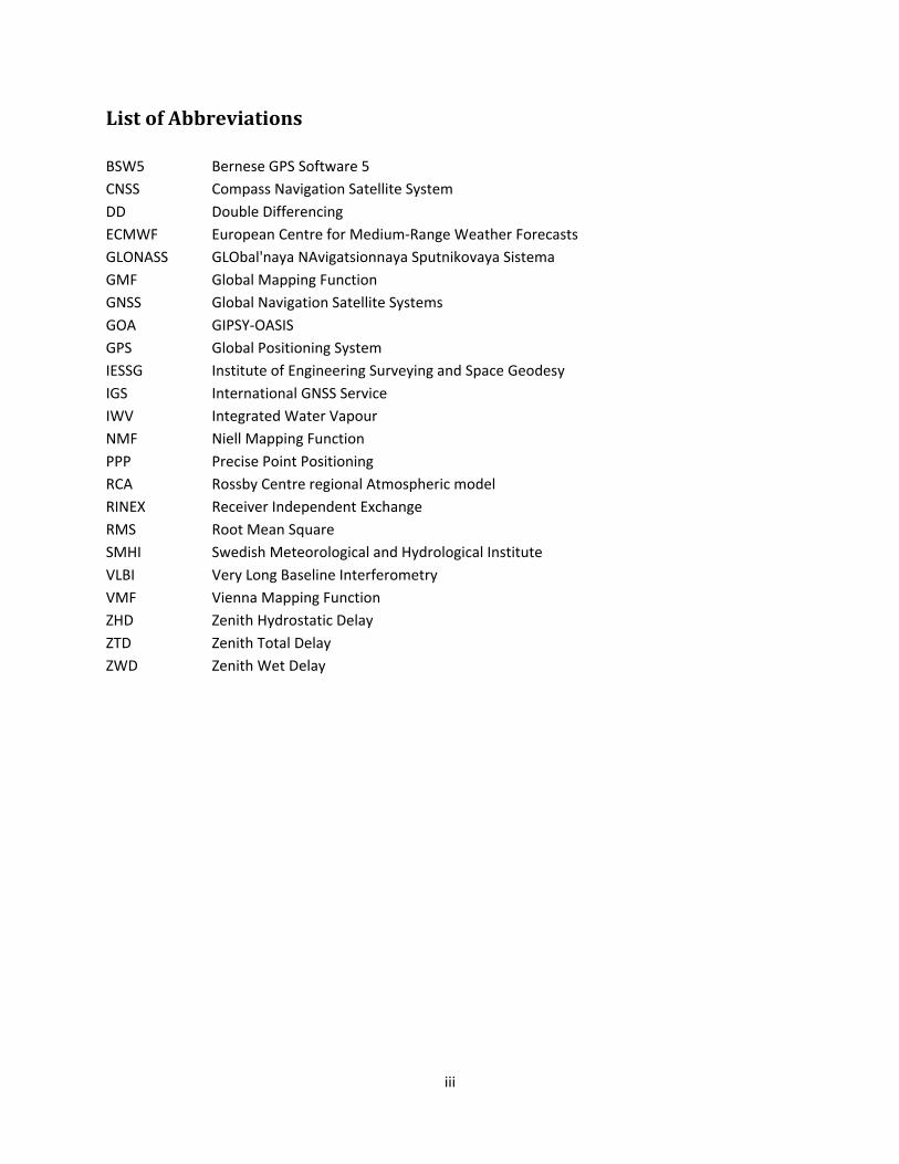
List of Abbreviations BSW5 Bernese GPS Software 5 CNSS Compass Navigation Satellite System DD Double Differencing ECMWF European Centre for Medium‐Range Weather Forecasts GLONASS GLObal'naya NAvigatsionnaya Sputnikovaya Sistema GMF Global Mapping Function GNSS Global Navigation Satellite Systems GOA GIPSY‐OASIS GPS Global Positioning System IESSG Institute of Engineering Surveying and Space Geodesy IGS International GNSS Service IWV Integrated Water Vapour NMF Niell Mapping Function PPP Precise Point Positioning RCA Rossby Centre regional Atmospheric model RINEX Receiver Independent Exchange RMS Root Mean Square SMHI Swedish Meteorological and Hydrological Institute VLBI Very Long Baseline Interferometry VMF Vienna Mapping Function ZHD Zenith Hydrostatic Delay ZTD Zenith Total Delay ZWD Zenith Wet Delay
iii

Contents Abstract .......................................................................................................................................................... i
Acknowledgements ....................................................................................................................................... ii
List of Abbreviations .................................................................................................................................... iii
Index of Tables ............................................................................................................................................ vii
Introduction to GNSS .................................................................................................................................... 1
1.1 Working of GNSS ................................................................................................................................. 1
1.1.1 Observables for GNSS ........................................................................................................... 1
1.2 Sources of error for GNSS ................................................................................................................... 2
1.2.1 Ionosphere ................................................................................................................................... 2
1.2.2 Troposphere ................................................................................................................................. 3
1.2.3 Clocks ........................................................................................................................................... 4
1.2.4 Orbits ............................................................................................................................................ 4
1.2.5 Phase Ambiguities ........................................................................................................................ 4
1.2.6 Geophysical Models ..................................................................................................................... 4
1.3 Applications of Global Navigation Satellite Systems .......................................................................... 5
1.4 Water Vapour Estimation using GNSS ................................................................................................ 5
1.4.1 Effect of Mapping Functions on Water Vapour Estimates .......................................................... 8
1.4.2 Effect of Antenna Phase Center Variation on Water Vapour Estimates ...................................... 9
1.4.3 Potential of Storm Tracking though GNSS ................................................................................... 9
Framework of the Project ........................................................................................................................... 10
2.1 The International GNSS Service ........................................................................................................ 10
2.2 Precise Point Positioning ................................................................................................................... 11
2.3 Double Difference Processing ........................................................................................................... 11
2.4 GNSS Data Processing ....................................................................................................................... 12
2.5 Description of the Tasks .................................................................................................................... 13
2.5.1 Software Comparison ................................................................................................................ 13
2.5.2 Simulations for GNSS ................................................................................................................. 14
2.5.3 Validation using Numerical Models ........................................................................................... 14
2.5.1 Criteria for Processing ................................................................................................................ 14
Software Comparison ................................................................................................................................. 16
3.1 Introduction to the Software Packages ............................................................................................ 16
iv
3.1.1 GPS Inferred Positioning SYstem – Orbit Analysis and Simulation Software ............................. 16
3.1.2 GAMIT GPS Analysis Software .................................................................................................... 16
3.1.3 Bernese GPS Software ............................................................................................................... 16
3.1.4 magicGNSS ................................................................................................................................. 16
3.2 Introduction to the Climate Models ................................................................................................. 17
3.2.1 European Centre for Medium‐Range Weather Forecasts Weather Model ............................... 17
3.2.2 Rossby Centre regional Atmospheric model .............................................................................. 17
3.3 Strategy for Comparison ................................................................................................................... 17
3.4 Results from Comparison .................................................................................................................. 17
3.4.1 Bilibino, Russian Federation (BILI) ............................................................................................. 17
3.4.2 Ulukhaktuk, Canada (HOLM) ...................................................................................................... 19
3.4.3 Kiruna, Sweden (KIR0) ................................................................................................................ 21
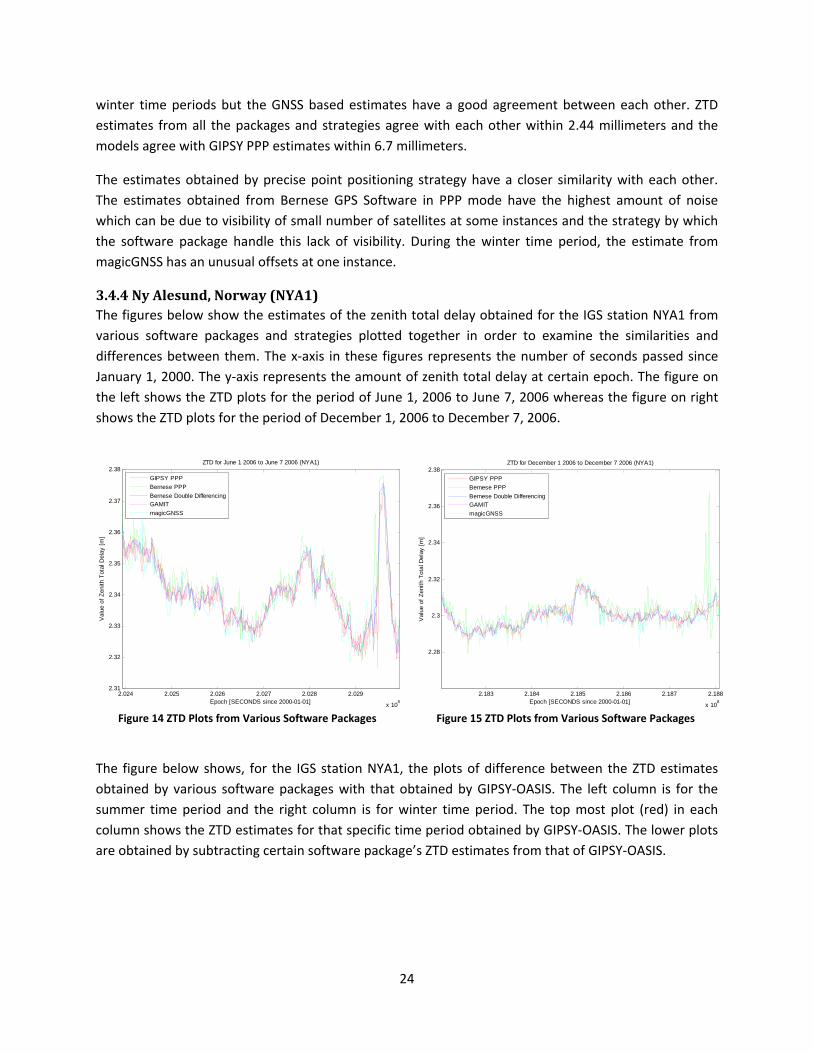
3.4.4 Ny Alesund, Norway (NYA1) ...................................................................................................... 24
3.4.5 Qaqortop, Greenland (QAQ1) .................................................................................................... 26
3.4.6 Resolute, Canada (RESO)............................................................................................................ 28
3.4.7 Reykjavik, Iceland (REYK) ........................................................................................................... 29
3.4.8 Scoresbysund, Greenland (SCOR) .............................................................................................. 31
3.4.9 Thule Airbase, Greenland (THU2) .............................................................................................. 34
3.4.10 Thule Airbase, Greenland (THU3) ............................................................................................ 36
3.4.11 Tromsoe, Norway (TRO1) ......................................................................................................... 38
3.4.12 Mean Differences as functions of Latitude, Longitude and Height ......................................... 40
3.5 Conclusions from Software Comparison .......................................................................................... 44
GNSS Simulation ......................................................................................................................................... 45
4.1 Motivation behind the Simulation .................................................................................................... 45
4.2 The Simulation Software ................................................................................................................... 45
4.3 Results from Simulation .................................................................................................................... 46
4.3.1 GPS ............................................................................................................................................. 46
4.3.2 GLONASS .................................................................................................................................... 47
4.3.3 The Galileo System ..................................................................................................................... 48
4.3.4 Combination of GPS, GLONASS and Galileo ............................................................................... 49
4.3.5 Different Inclinations for Galileo ................................................................................................ 50
4.3.6 New Semi‐Major Axis for Galileo ............................................................................................... 51
v

4.4 Conclusions from GNSS Simulations ................................................................................................. 51
Recommendations ...................................................................................................................................... 53
5.1 Recommendations from Software Comparison ............................................................................... 53
5.2 Recommendations from GNSS Simulations ...................................................................................... 53
Bibliography ................................................................................................................................................ 54
vi
vii
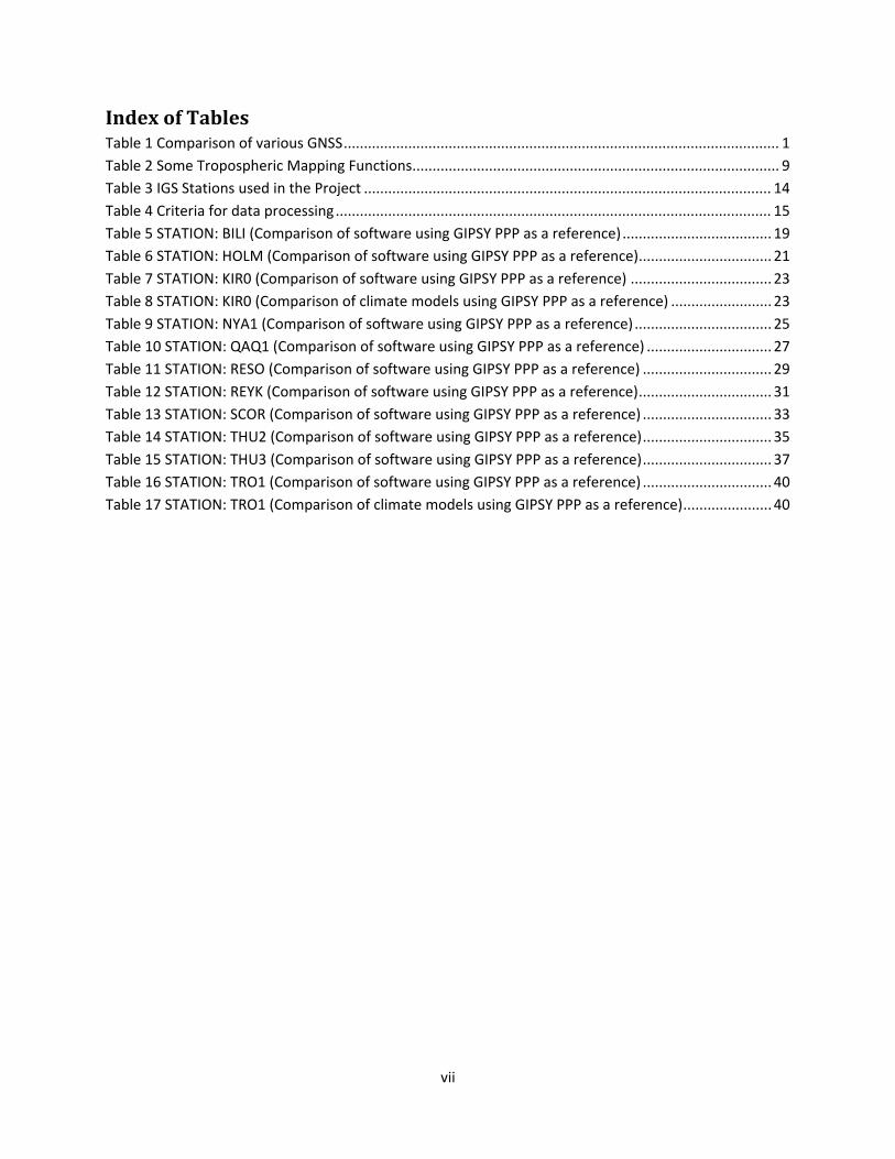
Index of Tables Table 1 Comparison of various GNSS ............................................................................................................ 1 Table 2 Some Tropospheric Mapping Functions........................................................................................... 9 Table 3 IGS Stations used in the Project ..................................................................................................... 14 Table 4 Criteria for data processing ............................................................................................................ 15 Table 5 STATION: BILI (Comparison of software using GIPSY PPP as a reference) ..................................... 19 Table 6 STATION: HOLM (Comparison of software using GIPSY PPP as a reference) ................................. 21 Table 7 STATION: KIR0 (Comparison of software using GIPSY PPP as a reference) ................................... 23 Table 8 STATION: KIR0 (Comparison of climate models using GIPSY PPP as a reference) ......................... 23 Table 9 STATION: NYA1 (Comparison of software using GIPSY PPP as a reference) .................................. 25 Table 10 STATION: QAQ1 (Comparison of software using GIPSY PPP as a reference) ............................... 27 Table 11 STATION: RESO (Comparison of software using GIPSY PPP as a reference) ................................ 29 Table 12 STATION: REYK (Comparison of software using GIPSY PPP as a reference) ................................. 31 Table 13 STATION: SCOR (Comparison of software using GIPSY PPP as a reference) ................................ 33 Table 14 STATION: THU2 (Comparison of software using GIPSY PPP as a reference) ................................ 35 Table 15 STATION: THU3 (Comparison of software using GIPSY PPP as a reference) ................................ 37 Table 16 STATION: TRO1 (Comparison of software using GIPSY PPP as a reference) ................................ 40 Table 17 STATION: TRO1 (Comparison of climate models using GIPSY PPP as a reference) ...................... 40
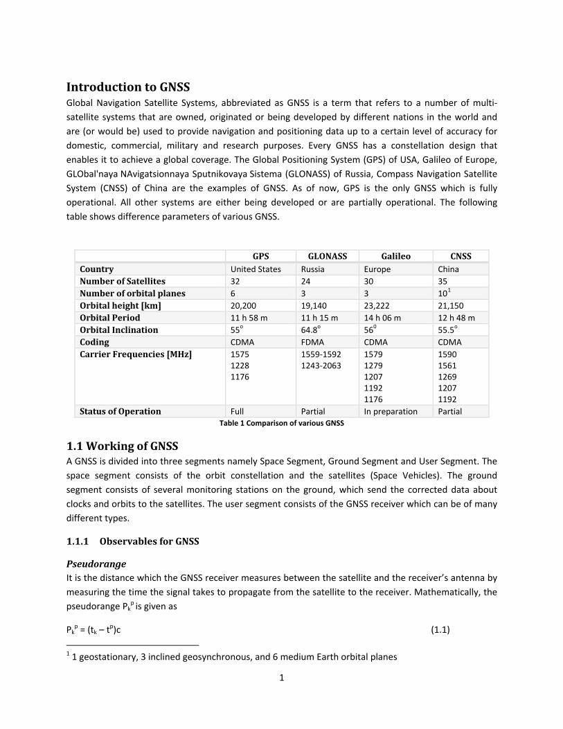
Introduction to GNSS Global Navigation Satellite Systems, abbreviated as GNSS is a term that refers to a number of multi‐satellite systems that are owned, originated or being developed by different nations in the world and are (or would be) used to provide navigation and positioning data up to a certain level of accuracy for domestic, commercial, military and research purposes. Every GNSS has a constellation design that enables it to achieve a global coverage. The Global Positioning System (GPS) of USA, Galileo of Europe, GLObal'naya NAvigatsionnaya Sputnikovaya Sistema (GLONASS) of Russia, Compass Navigation Satellite System (CNSS) of China are the examples of GNSS. As of now, GPS is the only GNSS which is fully operational. All other systems are either being developed or are partially operational. The following table shows difference parameters of various GNSS.
Table 1 Comparison of various GNSS
GPS GLONASS Galileo CNSSCountry United States Russia Europe ChinaNumber of Satellite s 32 24 30 35 Number of orbital planes 6 3 3 101 Orbital height km [ ] 20,200 19,140 23,222 21,150Orbital Period 11 h 58 m 11 h 15 m 14 h 06 m 12 h 48 mOrbital Inclination 55o 64.8o 560 55.5o
Coding CDMA FDMA CDMA CDMACarrier Frequencies [MHz] 1575
1228 1176
1559‐15921243‐2063
15791279 1207 1192 1176
15901561 1269 1207 1192
Status of Operation Full Partial In preparation Partial
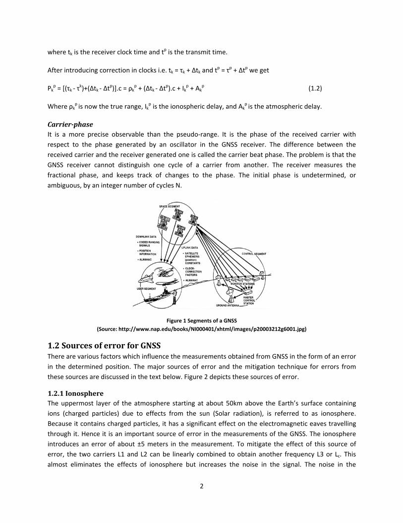
1.1 Working of GNSS A GNSS is divided into three segments namely Space Segment, Ground Segment and User Segment. The space segment consists of the orbit constellation and the satellites (Space Vehicles). The ground segment consists of several monitoring stations on the ground, which send the corrected data about clocks and orbits to the satellites. The user segment consists of the GNSS receiver which can be of many different types.
1.1.1 Observables for GNSS
Pseudorange It is the distance which the GNSS receiver measures between the satellite and the receiver’s antenna by measuring the time the signal takes to propagate from the satellite to the receiver. Mathematically, the pseudorange Pk
p is given as
Pkp = (tk – t
p)c (1.1)
1 1 geostationary, 3 inclined geosynchronous, and 6 medium Earth orbital planes
1
where tk is the receiver clock time and tp is the transmit time.
After introducing correction in clocks i.e. tk = τk + Δtk and tp = τp + Δtp we get
Pkp = [(τk ‐ τ
k)+(Δtk ‐ Δtp)].c = ρk
p + (Δtk ‐ Δtp).c + Ik
p + Akp (1.2)
Where ρkp is now the true range, Ik
p is the ionospheric delay, and Akp is the atmospheric delay.
Carrierphase It is a more precise observable than the pseudo‐range. It is the phase of the received carrier with respect to the phase generated by an oscillator in the GNSS receiver. The difference between the received carrier and the receiver generated one is called the carrier beat phase. The problem is that the GNSS receiver cannot distinguish one cycle of a carrier from another. The receiver measures the fractional phase, and keeps track of changes to the phase. The initial phase is undetermined, or ambiguous, by an integer number of cycles N.
Figure 1 Segments of a GNSS (Source: http://www.nap.edu/books/NI000401/xhtml/images/p20003212g6001.jpg)
1.2 Sources of error for GNSS There are various factors which influence the measurements obtained from GNSS in the form of an error in the determined position. The major sources of error and the mitigation technique for errors from these sources are discussed in the text below. Figure 2 depicts these sources of error.
1.2.1 Ionosphere The uppermost layer of the atmosphere starting at about 50km above the Earth’s surface containing ions (charged particles) due to effects from the sun (Solar radiation), is referred to as ionosphere. Because it contains charged particles, it has a significant effect on the electromagnetic eaves travelling through it. Hence it is an important source of error in the measurements of the GNSS. The ionosphere introduces an error of about ±5 meters in the measurement. To mitigate the effect of this source of error, the two carriers L1 and L2 can be linearly combined to obtain another frequency L3 or Lc. This almost eliminates the effects of ionosphere but increases the noise in the signal. The noise in the
2
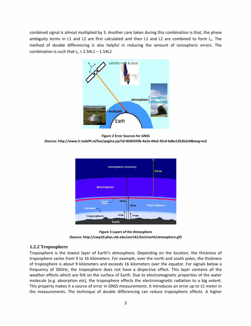
combined signal is almost multiplied by 3. Another care taken during this combination is that, the phase ambiguity terms in L1 and L2 are first calculated and then L1 and L2 are combined to form Lc. The method of double differencing is also helpful in reducing the amount of ionospheric errors. The combination is such that Lc = 2.54L1 – 1.54L2
Figure 2 Error Sources for GNSS (Source: http://www.lr.tudelft.nl/live/pagina.jsp?id=8584359b‐4e2a‐44a2‐92cd‐6dbe12b2b2a9&lang=en)
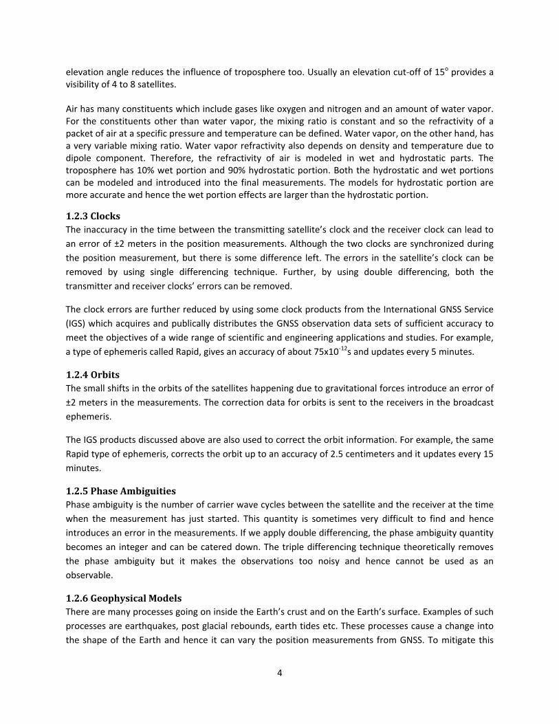
Figure 3 Layers of the Atmosphere (Source: http://csep10.phys.utk.edu/astr161/lect/earth/atmosphere.gif)
1.2.2 Troposphere Troposphere is the lowest layer of Earth’s atmosphere. Depending on the location, the thickness of troposphere varies from 9 to 16 kilometers. For example, over the north and south poles, the thickness of troposphere is about 9 kilometers and exceeds 16 kilometers over the equator. For signals below a frequency of 30GHz, the troposphere does not have a dispersive effect. This layer contains all the weather effects which are felt on the surface of Earth. Due to electromagnetic properties of the water molecule (e.g. absorption etc), the troposphere effects the electromagnetic radiation to a big extent. This property makes it a source of error in GNSS measurements. It introduces an error up to ±1 meter in the measurements. The technique of double differencing can reduce tropospheric effects. A higher
3
elevation angle reduces the influence of troposphere too. Usually an elevation cut‐off of 15o provides a visibility of 4 to 8 satellites. Air has many constituents which include gases like oxygen and nitrogen and an amount of water vapor. For the constituents other than water vapor, the mixing ratio is constant and so the refractivity of a packet of air at a specific pressure and temperature can be defined. Water vapor, on the other hand, has a very variable mixing ratio. Water vapor refractivity also depends on density and temperature due to dipole component. Therefore, the refractivity of air is modeled in wet and hydrostatic parts. The troposphere has 10% wet portion and 90% hydrostatic portion. Both the hydrostatic and wet portions can be modeled and introduced into the final measurements. The models for hydrostatic portion are more accurate and hence the wet portion effects are larger than the hydrostatic portion.
1.2.3 Clocks The inaccuracy in the time between the transmitting satellite’s clock and the receiver clock can lead to an error of ±2 meters in the position measurements. Although the two clocks are synchronized during the position measurement, but there is some difference left. The errors in the satellite’s clock can be removed by using single differencing technique. Further, by using double differencing, both the transmitter and receiver clocks’ errors can be removed.
The clock errors are further reduced by using some clock products from the International GNSS Service (IGS) which acquires and publically distributes the GNSS observation data sets of sufficient accuracy to meet the objectives of a wide range of scientific and engineering applications and studies. For example, a type of ephemeris called Rapid, gives an accuracy of about 75x10‐12s and updates every 5 minutes.
1.2.4 Orbits The small shifts in the orbits of the satellites happening due to gravitational forces introduce an error of ±2 meters in the measurements. The correction data for orbits is sent to the receivers in the broadcast ephemeris.
The IGS products discussed above are also used to correct the orbit information. For example, the same Rapid type of ephemeris, corrects the orbit up to an accuracy of 2.5 centimeters and it updates every 15 minutes.
1.2.5 Phase Ambiguities Phase ambiguity is the number of carrier wave cycles between the satellite and the receiver at the time when the measurement has just started. This quantity is sometimes very difficult to find and hence introduces an error in the measurements. If we apply double differencing, the phase ambiguity quantity becomes an integer and can be catered down. The triple differencing technique theoretically removes the phase ambiguity but it makes the observations too noisy and hence cannot be used as an observable.
1.2.6 Geophysical Models There are many processes going on inside the Earth’s crust and on the Earth’s surface. Examples of such processes are earthquakes, post glacial rebounds, earth tides etc. These processes cause a change into the shape of the Earth and hence it can vary the position measurements from GNSS. To mitigate this
4

source of error, the processes can be modeled and their effects can be truncated from the position measurements.
These models can be adaptive i.e. different for different regions on the Earth. For example, if we consider Earth tides phenomena, displacements caused by ocean tidal loading are more than the displacements due to the earth body tide. Hence different models should be used for both of them.
The products from IGS, also provide some adjustment for Earth’s rotation. They can provide Polar Motion, Polar Motion Rates and Length‐of‐Delay.
1.3 Applications of Global Navigation Satellite Systems Global Navigation Satellite Systems are used or can be used for a multitude of different applications many well‐connected to our daily life. Several of those are developed through interdisciplinary research. Examples are found in geophysics, road construction, weather forecasting, warning systems for detection of movements in constructions, navigation, tracking of transports, climate studies, time and frequency transfer for national time keeping, earthquake studies, frequency synchronization for TV and communication networks, solar studies and space weather.
The International GNSS Service (IGS) network of globally distributed GNSS tracking stations is continuously used for the establishment and maintenance of the reference systems, weather and climate monitoring, and in geophysical applications. The IGS network was established in 1994 and currently consists of more than 200 stations spread all over the world. The data is available, free of charge over the internet.
1.4 Water Vapour Estimation using GNSS As discussed above, when a GNSS signal travels through various layers of the atmosphere, it experiences a certain amount of delay due to the content of a certain layer. For example, as the signal travels through the troposphere, the presence of water molecule in troposphere introduces a delay in the signal propagation. Hence, the amount of delay in troposphere is directly related to the amount of water molecule in the troposphere. Therefore, a careful observation of the delay in the signal can give a realistic estimate of the water vapor. This virtue is exploited to use GNSS in atmospheric water vapor estimation and in turn climate research (Bevis et al., 1992). The following text provides an overview of how can GNSS signals can be used to estimate water vapor.
Refractive index for a medium is defined as the ratio of speed of light in vacuum to the speed of light in that particular medium. Hence when a signal is travelling through a particular medium, its refractive index has an influence on the speed of propagation of the signal. Different layers of atmosphere have different refractive indices and when a GNSS signal travels through a layer, it experiences a delay in propagation due to the refractive properties of that layer.
If we assume a refractive index of n in the atmosphere, then the electrical path length L of a signal a path S is defined as
5
propagating along
(1.3)
Where the path S is determined from the index of refraction in the atmosphere using Fermat’s Principle which states that the signal will propagate along the path that gives minimum value of L. The geometrical straight line distance G through the atmosphere is always shorter than the path S of the propagated signal. The electrical path length of the signal propagating along G is longer than that for the signal propagating along S.
The difference between the electrical path length and the geometrical straight line distance is called s path, path delay, or simply delay: exces propagation
(1.4)
We may rewrite this expressi
1 (1.5)
on as
where S = ∫s ds. The (S‐G) term is often referred to as the geometric delay or the delay due to bending,
g and denoted as ΔL
∆ (1.6)
If the atmosphere is horizontally stratified, S and G are identical in the zenith direction and hence the geometric delay becomes equal to zero at this angle. (typically 3 cm at an elevation angle of 10°and 10 cm at 5°).
The delay due to hydrostatic part of the troposphere is also known as the dry delay. So we can express the refractivity of air in terms of density.
(1.7)
where
22.1 2.2 ⁄
The first term in the above equation is the dry part of the refractivity (Ndry) and second term is the wet part of the refractivity (Nwet). Where k1 = 77.60 +/‐ 0.05 K/mbar, k2 = 70.4 +/‐ 2.2 K/mbar, k3 = (3.730+/‐0.012)x10
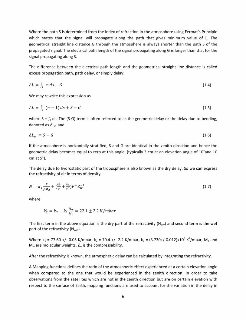
5 K2/mbar, Md and Mw are molecular weights, Zw is the compressability. After the refractivity is known, the atmospheric delay can be calculated by integrating the refractivity. A Mapping functions defines the ratio of the atmospheric effect experienced at a certain elevation angle when compared to the one that would be experienced in the zenith direction. In order to take observations from the satellites which are not in the zenith direction but are on certain elevation with respect to the surface of Earth, mapping functions are used to account for the variation in the delay in
6
different directions. There are different mapping functions for the wet and hydrostatic parts of the atmosphere but for low elevation angles, the same mapping function can be used for both the wet and hydrostatic parts.
Figure 4 Illustration of Elevation Dependence (Source: Lecture Slides by Dr. Jan Johansson)
The delay term can be expressed using the ydrostatic and the wet mapping func ions. ∆ (1.8)
h t
Where mh and mw are the hydrostatic and wet mapping functions. A sim le ex
1sin (1.9)
p ample of a mapping function can look like
where is the elevation angle. Nowadays, mapping functions are expressed in form of a continued fraction, for example (Herring 1992),
(1.10)
In the above form of a mapping function, the coefficients a, b and c depend on parameters like location of the station and the day of the year so that the seasonal variation within the troposphere is accounted for. The value of these coefficients can be derived from theoretical atmospheric models, numerical weather models or local measurements of pressure and temperature etc. The mapping function can be included in the delay measurements as shown in the following equation.
7
∆ 1 10 (1.11)

In the above equation, atm is the electrical path of the signal, vac is the geometrical straight path of the signal z is station height and m( ) is the mapping function to account for gradients in the atmosphere.
term ry et of the delay, Now, in s of d and w parts ∆ ∆ ∆ (1.12) Hence, the atmospheric delay can be divided into a hydrostatic part and a wet part. Both of these parts have their separate mapping functions. The integration of refractivity in vertical direction gives a quantity named as the zenith delay. Following the above discussion, the zenith delay is further divided into zenith hydrostatic delay (ZHD) and zenith wet delay (ZWD).
∆ ∆
The quantity zenith to
(1.13) tal delay (ZTD) can then be defined as
If certain parameters (e.g. pressure, temperature etc) are know, the ZWD can be mapped onto Integrated Water Vapor (IWV) in the atmosphere (Bevis et al., 1994) which is used in climate research.
Figure 5 Obtaining IWV from GNSS Observations
1.4.1 Effect of Mapping Functions on Water Vapour Estimates A mapping function is defined as the ratio between amount of propagation delay at different elevation angles to the that in the zenith direction. The purpose of a mapping function is to account for the variation in the delay as a function of elevation angle. There are various mapping functions available for this purpose and a continuous research is on the way to improve and devise mapping functions. For example, a mapping function which models the atmosphere in terms of azimuth angle was suggested by Orilac et al., 2006.
In this project, Niell Mapping Function or NMF (Niell 1996) has been used. This model has a hydrostatic part and a wet part. The hydrostatic part depends on the latitude of the station, its height above sea
8
level and the day of the year. The wet part of NMF depends upon the station latitude. NMF was developed for Very Long Baseline Interferometery (VLBI) purposes but has also been adopted and is widely used for GPS processing.
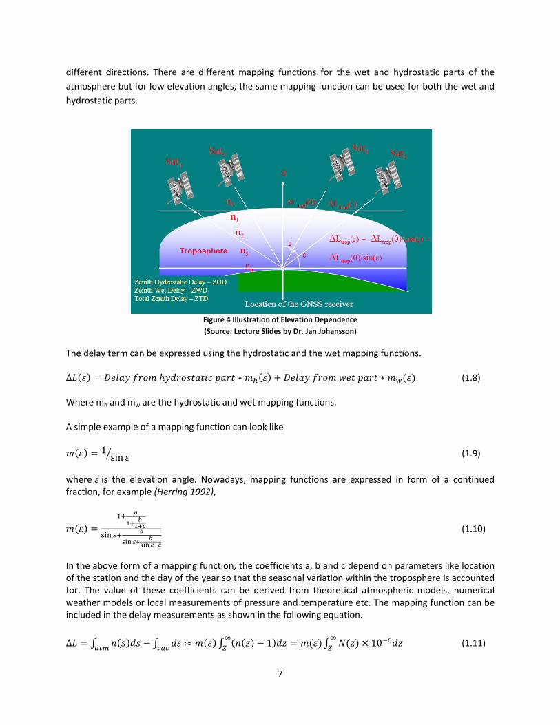
The following table gives an overview of some mapping functions in use currently.
Name Developed by Year Dependence
Niell Mapping Function (NMF)
A E Niell 1996 Latitude, Height, Day of Year
Global Mapping Function J. Boehm et al 2006 Numerical Weather Model VMF1 J. Boehm et al 2006 Ray Tracing through Atmosphere
Table 2 Some Tropospheric Mapping Functions
1.4.2 Effect of Antenna Phase Center Variation on Water Vapour Estimates GNSS Meteorology is a growing field and research is going on to improve the accuracy of data obtained from GNSS. For instance, techniques are being developed to eliminate the effect of antenna phase center variations. When a GNSS receiver antenna receives signal from different elevation and azimuth angles, the electrical phase center of the antenna varies for every angle and hence the signal is affected. It has been shown that if GPS data is used without inclusion of appropriate antenna models, errors are induced in water vapour estimates (Jarlemark et al., 2010). New models for the antennas such as the absolute antenna calibration models are being developed to truncate the influence of phase center variations (Gorres et al., 2005). In 2006, IGS adopted the absolute antenna calibration model for its network and it resulted in an improvement in the water vapour estimates and elimination of the systematic errors which previously caused an overestimation in water vapour content (Ortiz de Galisteo et al., 2010). Techniques can also be developed to reduce the elevation dependent effects like scattering and multipath reflections to improve the estimates of water vapour (Ning et al., 2010).
1.4.3 Potential of Storm Tracking though GNSS Utilizing its capability of water vapour estimation, GNSS has a potential to detect and track extreme changes in weather such as thunderstorms. As an example, the Institute of Engineering Surveying and Space Geodesy (IESSG) at the University of Nottingham has developed a near‐real time processing system for GPS based on Bernese GPS Software 5. This system used a dense network of stations within Europe and was operationally tested by United Kingdom’s Met Office. The potential of the system was demonstrated by performing two case studies in which GPS observations were compared with those obtained from Weather Radar and Satellite Imagery. The comparison validated the GPS observations (Nash et al., 2006).
9
Framework of the Project
2.1 The International GNSS Service
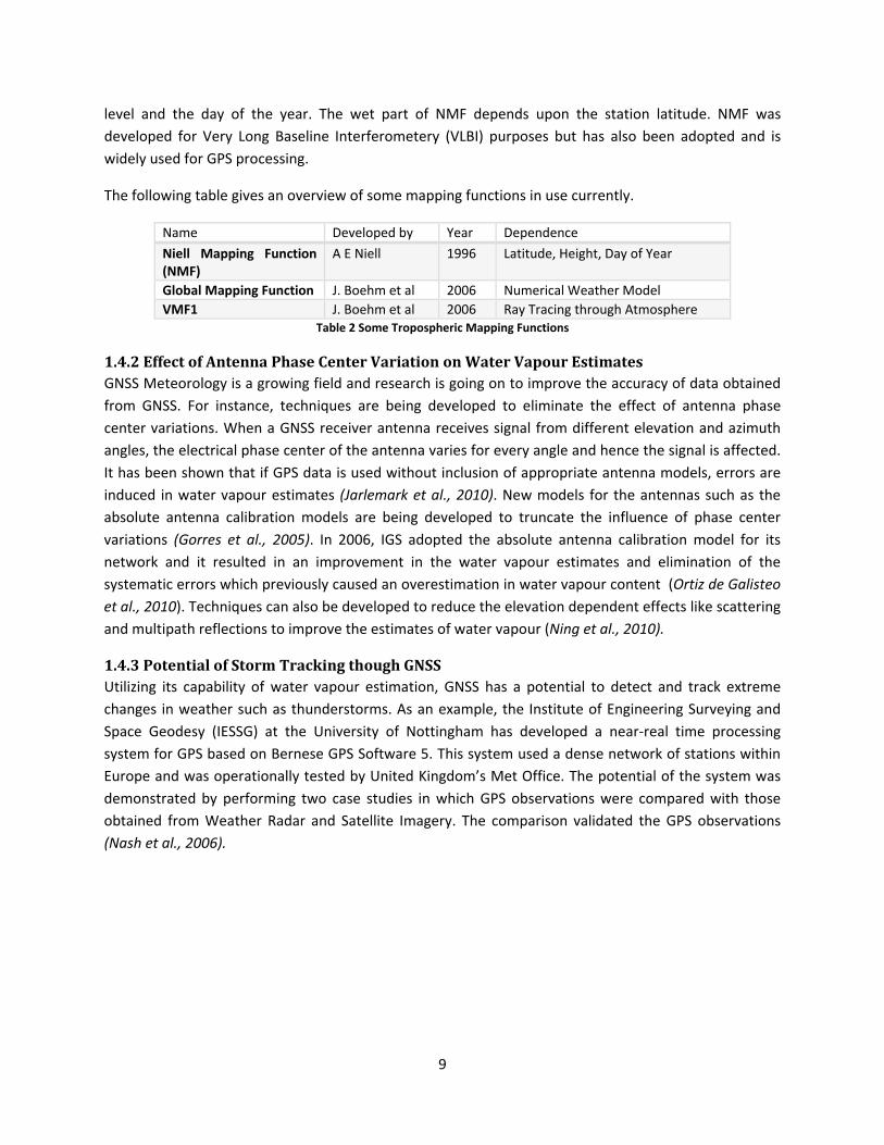
The International GNSS Service (Dow et al., 2009) or IGS is a non‐profit alliance of a huge number of research agencies worldwide that own and operate permanent GNSS receiver stations in order to produce products to enhance the accuracy of GNSS observations. In addition to providing raw measurements from GNSS, the IGS contributes to the maintenance and improvement of the International Terrestrial Reference Frame, produces high accuracy satellite orbit and clock data, and monitors the Earth's rotation and the state of its ionized and neutral atmospheres. As mentioned earlier, GNSS technology is being used in Earth science research and other multidisciplinary applications, hence, the products from IGS can be used to improve the quality and reliability of the processes and the research. Currently, the IGS network deals with two types of GNSS namely the GPS and GLONASS. The data and products from IGS network are available free of cost over the internet and the agencies in the IGS network operate without any contract or regulations. The figure below shows the network of core receiver stations used by IGS in order to generate the products.
Figure 6 Network of IGS Reference Stations (Source: www.igscb.jpl.nasa.gov)
Examples of some agencies in the IGS are Jet Propulsion Laboratory (USA), University of Bern (Switzerland), SCRIPPS Institute of Oceanography (USA), and GMV (Spain) etc. All the agencies in IGS generate their products by using a common network of 50 core reference stations spread all over the globe. As it would be addressed later in the text, different software packages available for GNSS data processing use the products from different IGS agencies and for each agency, the level of precision in the products is different. This difference can influence the data analysis up to some extent.
10

2.2 Precise Point Positioning Precise Point Positioning or PPP is a strategy of processing the data to obtain coordinates by using only one receiver (Zumberge et al., 1997). In this strategy, high precision information about satellite orbits, satellite and receiver clocks and Earth orientation parameters is obtained from the IGS network for every epoch. This information is then used to apply the error correction for each epoch in order to obtain precise coordinates.
The figure below depicts the principle behind PPP.
Figure 7 Illustration of Precise Point Positioning
2.3 Double Difference Processing Double Difference Processing or DD (Hofmann‐Wellenhof et al., 2001) is another strategy of determination of coordinates by removing the clock errors. In this strategy, the coordinates are solved for a baseline relative to a station with well known coordinates. The equations for solving the coordinates are formed by taking differences between the receivers and the satellites. For double difference processing, the observations from two satellites at known locations can be differenced and/or a same satellite can be observed from two receivers at known locations.
The following figure depicts the principle behind Double Differencing.
11

Figure 8 Illustration of Double Difference Processing
2.4 GNSS Data Processing The raw observations from GNSS are obtained in Receiver Independent Exchange (RINEX) format which are processed using GNSS data processing software packages to obtain the desired output in form of spatial coordinates and atmospheric delay etc. For processing using a software package, the raw data first undergoes editing and decimation. Along with the edited data, information about satellite positions in orbits, satellite clocks, a priori coordinates of the ground receiver and values from geophysical models etc are fetched from various sources. One primary source is the International GNSS Service. A combination of edited data and fetched information is then fed to the processing engine of the software package which is based on different techniques for different package. Kalman filter and Least square averaging are examples of such techniques. During the processing, the available information about errors from various error sources is used to correct the a priori values and an output is generated after the correction of these errors. The output generated includes spatial coordinates, clock bias and tropospheric delay components. The following figure provides an overview of GNSS data processing.
12
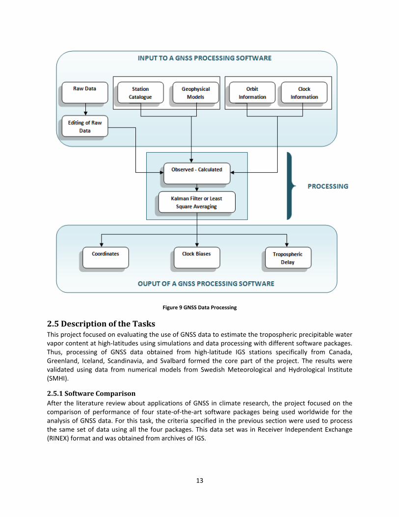
Figure 9 GNSS Data Processing
2.5 Description of the Tasks This project focused on evaluating the use of GNSS data to estimate the tropospheric precipitable water vapor content at high‐latitudes using simulations and data processing with different software packages. Thus, processing of GNSS data obtained from high‐latitude IGS stations specifically from Canada, Greenland, Iceland, Scandinavia, and Svalbard formed the core part of the project. The results were validated using data from numerical models from Swedish Meteorological and Hydrological Institute (SMHI).
2.5.1 Software Comparison After the literature review about applications of GNSS in climate research, the project focused on the comparison of performance of four state‐of‐the‐art software packages being used worldwide for the analysis of GNSS data. For this task, the criteria specified in the previous section were used to process the same set of data using all the four packages. This data set was in Receiver Independent Exchange (RINEX) format and was obtained from archives of IGS.
13
2.5.2 Simulations for GNSS As discussed above, there are still some Global Navigation Satellite Systems which are either under development or are partly operational. For such systems, simulations have been carried out during this project using an in‐house software package developed at Chalmers University of Technology and SP Technical Research Institute of Sweden. The simulations have provided measure of errors in zenith wet delay for different systems. Along with simulating new systems, a combination of different systems has also been simulated.
2.5.3 Validation using Numerical Models Once the data have been processed using GNSS processing software packages, the value of zenith total delay for the same time period in the criteria has been compared to that obtained by using other conventional methods for water vapor estimation for the purpose of validation. This data was provided by the Swedish Meteorological and Hydrological Institute (SMHI).
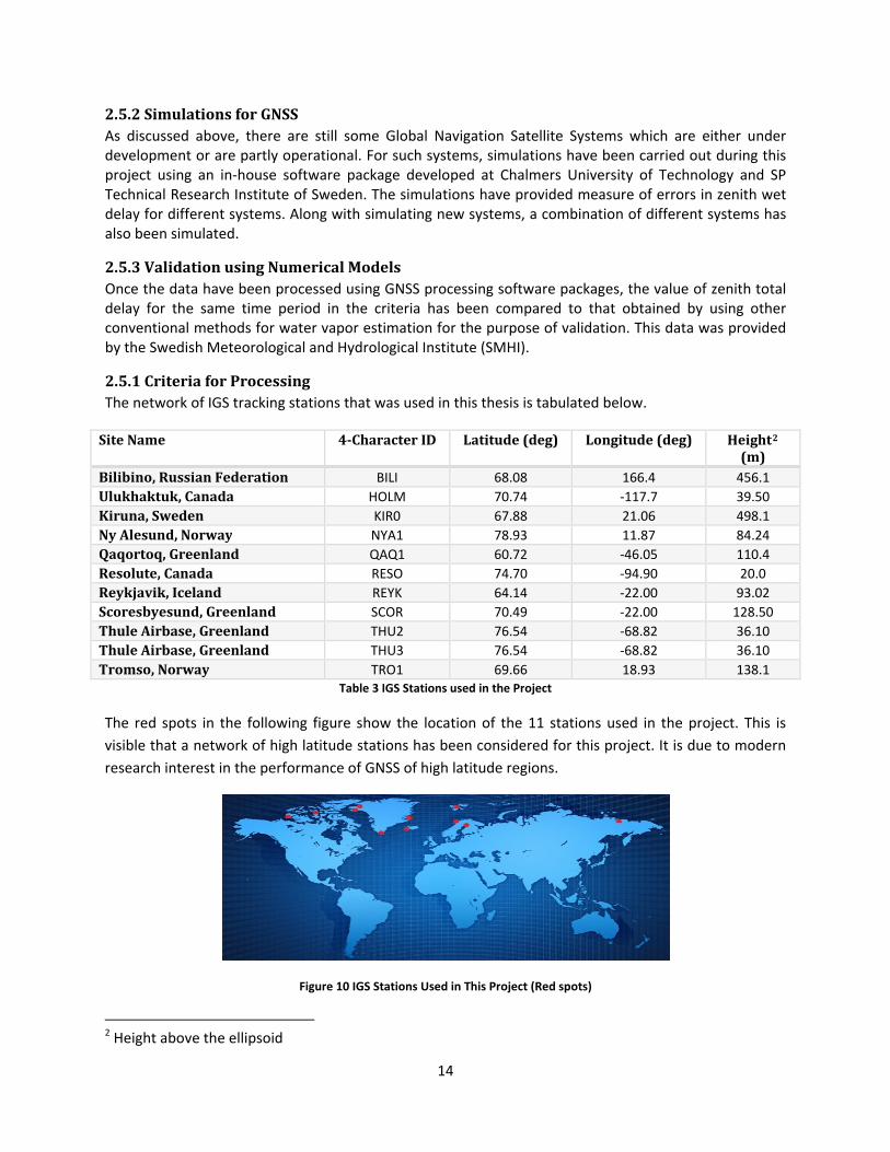
2.5.1 Criteria for Processing The network of IGS tracking stations that was used in this thesis is tabulated below.
Site Name 4Character ID Latitude (deg) Longitude (deg) Height2 (m)
Bilibino, Russian Federation BILI 68.08 166.4 456.1Ulukhaktuk, Canada HOLM 70.74 ‐117.7 39.50Kiruna, Sweden KIR0 67.88 21.06 498.1Ny Alesund, Norway NYA1 78.93 11.87 84.24Qaqortoq, Greenland QAQ1 60.72 ‐46.05 110.4Resolute, Canada RESO 74.70 ‐94.90 20.0Reykjavik, Iceland REYK 64.14 ‐22.00 93.02Scoresbyesund, Greenland SCOR 70.49 ‐22.00 128.50Thule Airbase, Greenland THU2 76.54 ‐68.82 36.10Thule Airbase, Greenland THU3 76.54 ‐68.82 36.10Tromso, Norway TRO1 69.66 18.93 138.1
Table 3 IGS Stations used in the Project
The red spots in the following figure show the location of the 11 stations used in the project. This is visible that a network of high latitude stations has been considered for this project. It is due to modern research interest in the performance of GNSS of high latitude regions.
Figure 10 IGS Stations Used in This Project (Red spots)
2 Height above the ellipsoid
14

Other parameters in the criteria are listed below.
Parameter Value Time Period (Summer) June 1, 2006 to June 7, 2006Time Period (Winter) December 1, 2006 to December 7, 2006 Data Acquired Zenith Total DelayMapping Functions Used Niell Mapping FunctionClimate Models Used ECMWF, RCAAntenna Phase Center Correction Absolute Calibration ModelsElevation Cut Off 10o
Table 4 Criteria for data processing
The choice of elevation cut‐off angle is a tradeoff between noisy observations and good satellite geometry. For the sake of visibility of all the satellites above the horizon, very low elevation cut‐off angle is needed. But the lower the cut‐off angle is, more is the signal influenced by atmospheric and multipath effects. Therefore, for this project, an elevation angle of 10o was chosen being a reasonable choice. The time period used to process the data from consisted of two weeks in year 2006 i.e. first 7 days of both June and December. These periods were selected keeping in view of the availability of complete data set for all 11 stations during these periods. The tropospheric mapping function used in this project was the Niell Mapping Function due to the fact the all the software packages to be compared can handle this mapping function and that this mapping function is suitable to use with the chosen elevation cut‐off. Some other mapping function could have been used if the elevation cut‐off value was chosen to be lower. The correction in antenna phase center variations were handled by adopting absolute antenna calibration models from the IGS. Along with the four software packages, a regional climate model called the Rossby Centre regional Atmospheric model (RCA) and a global weather model from European Centre for Medium‐Range Weather Forecasts (ECMWF) were used to obtain the zenith total delay estimates for the selected time periods.
15

Software Comparison This chapter describes the first part of the project and presents results, conclusions, discussion and recommendations which emerged after this part.
3.1 Introduction to the Software Packages In the following text, the four GNSS data processing software packages that were compared during this part of the project are introduced briefly.
3.1.1 GPS Inferred Positioning SYstem – Orbit Analysis and Simulation Software GPS Inferred Positioning System – Orbit Analysis and Simulation Software or GIPSY‐OASIS (GOA) is a software package developed by Jet Propulsion Laboratory at California Institute of Technology, USA (Zumberge et al., 1997). This package runs in UNIX environment and is based on the Kalman Filter technique. For this project, the version 5.0 of this package was used at Chalmers University of Technology. To process the data set with this package, the strategy of precise point positioning (PPP) was adopted and error correction products from IGS were used.
This software package, in its various versions, has been used by Geodesy and Geodynamics Group at Onsala Space Observatory (Chalmers University of Technology) since 20 years.
3.1.2 GAMIT GPS Analysis Software GAMIT GPS Analysis Software (Herring, 2005) is a software package developed by Department of Earth Atmospheric and Planetary Sciences at Massachusetts Institute of Technology, USA. This package runs in UNIX environment and is based on the Kalman Filter technique. For this project, the version 10.35 of this package was used at National Land Survey of Sweden. To process the data set with this package, the strategy of Double Difference processing (DD) was adopted and error correction products from IGS were used.
3.1.3 Bernese GPS Software Bernese GPS Software (BSW) is a software package developed by University of Berne, Switzerland (Dach et al., 2007). This package can run in both Microsoft Windows and UNIX environments and is based on Least Squares Fit technique. For this project, the version 5.0 of this package was used at National Land Survey of Sweden. This package is capable of handling both the precise point positioning and the double difference processing strategies and hence, to process the data set with this package, both of these strategies were adopted and error correction products from IGS were used.
3.1.4 magicGNSS This is a commercial software package developed by GMV Aerospace and Defense S.A., Spain (Mozo, A. et al 2008). A non‐commercial version of this package is being used by the European Space Agency for the Galileo project. As this is a commercial software, a special online access to the version 2.5 of this package was obtained to process the data set for this project. Being an online software, it can be used easily on any web browser. This package was used to process the data using precise point positioning technique.
16

3.2 Introduction to the Climate Models In this section, the climate and weather models used for the validation of output from GNSS software packages are introduced.
3.2.1 European Centre for MediumRange Weather Forecasts Weather Model The weather model from European Centre for Medium‐Range Weather Forecasts (ECMWF) is a global model for numerical weather predictions (Jung, T. et al., 2010). For this project, the zenith total delay values from this model were obtained to compare them with those obtained from the software packages. The values from this model were provided by Swedish Meteorological and Hydrological Institute (SMHI), Sweden.
3.2.2 Rossby Centre regional Atmospheric model The Rossby Centre regional Atmospheric model (RCA) from Rossby Centre, SMHI is a regional climate model (Achberger, C. et al., 2003). This model is a specialized form of the ECMWF model with implemented boundary conditions and a regional scope for Nordic region. The RCA model has a higher resolution as compared to that of the ECMWF model. For this project, the zenith total delay values from this model were obtained to compare them with those obtained from the software packages. The values from this model were provided by Swedish Meteorological and Hydrological Institute, Sweden.
3.3 Strategy for Comparison As discussed in the previous sections, the values of zenith total delay for the chosen time periods were obtained using all the four software packages (for all 11 stations) and the two models (for 2 stations). GOA, BSW, magicGNSS and the two models produced an output with the value of zenith total delay every 5 minutes whereas GAMIT estimated the zenith total delay every 1 hour. Once obtained, these values were plotted against time in a single figure to observe the similarities and differences. After this, a statistical comparison between outputs of different techniques was performed. For this comparison, the output from GOA software package was selected as a reference and the difference between GOA output and output from every other technique was analyzed. For example, to compare the output of BSW with the output of GOA, it was subtracted from the output of GOA and then this difference (bias) was examined by taking its mean and standard deviation. These biases were plotted and the statistics were presented in tabular form.
3.4 Results from Comparison This section presents the results from the software comparison part of the project.
3.4.1 Bilibino, Russian Federation (BILI) The figures below show the estimates of the zenith total delay obtained for the IGS station BILI from various software packages and strategies plotted together in order to examine the similarities and differences between them. The x‐axis in these figures represents the number of seconds passed since January 1, 2000. The y‐axis represents the amount of zenith total delay at certain epoch. The figure on the left shows the ZTD plots for the period of June 1, 2006 to June 7, 2006 whereas the figure on right shows the ZTD plots for the period of December 1, 2006 to December 7, 2006.
17
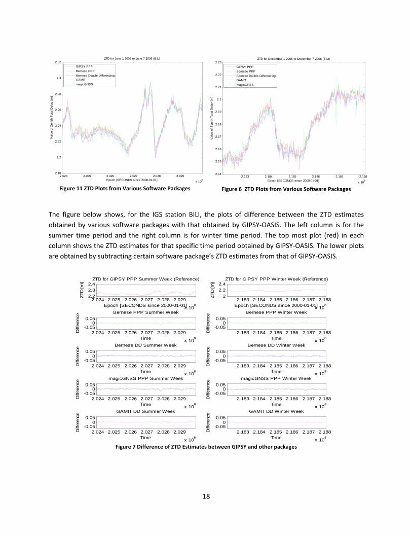
Figure 11 ZTD Plots from Various Software Packages
Figure 6 ZTD Plots from Various Software Packages
The figure below shows, for the IGS station BILI, the plots of difference between the ZTD estimates obtained by various software packages with that obtained by GIPSY‐OASIS. The left column is for the summer time period and the right column is for winter time period. The top most plot (red) in each column shows the ZTD estimates for that specific time period obtained by GIPSY‐OASIS. The lower plots are obtained by subtracting certain software package’s ZTD estimates from that of GIPSY‐OASIS.
Figure 7 Difference of ZTD Estimates between GIPSY and other packages
2.024 2.025 2.026 2.027 2.028 2.029
x 108
2.18
2.2
2.22
2.24
2.26
2.28
2.3
2.32
Epoch [SECONDS since 2000-01-01]
Val
ue o
f Zen
ith T
otal
Del
ay [m
]
ZTD for June 1 2006 to June 7 2006 (BILI)
GIPSY PPPBernese PPPBernese Double DifferencingGAMITmagicGNSS
2.183 2.184 2.185 2.186 2.187 2.188
x 108
2.14
2.15
2.16
2.17
2.18
2.19
2.2
2.21
2.22
2.23
Epoch [SECONDS since 2000-01-01]
Val
ue o
f Zen
ith T
otal
Del
ay [m
]
ZTD for December 1 2006 to December 7 2006 (BILI)
GIPSY PPPBernese PPPBernese Double DifferencingGAMITmagicGNSS
2.024 2.025 2.026 2.027 2.028 2.029
x 108
2.22.32.4
ZTD for GIPSY PPP Summer Week (Reference)
Epoch [SECONDS since 2000-01-01]
ZTD
[m]
2.183 2.184 2.185 2.186 2.187 2.188
x 108
22.22.4
ZTD for GIPSY PPP Winter Week (Reference)
Epoch [SECONDS since 2000-01-01]
ZTD
[m]
2.183 2.184 2.185 2.186 2.187 2.188
x 108
-0.050
0.05Bernese PPP Winter Week
Time
Diff
eren
ce
2.024 2.025 2.026 2.027 2.028 2.029
x 108
-0.050
0.05Bernese PPP Summer Week
Time
Diff
eren
ce
2.183 2.184 2.185 2.186 2.187 2.188
x 108
-0.050
0.05Bernese DD Winter Week
Time
Diff
eren
ce
2.024 2.025 2.026 2.027 2.028 2.029
x 108
-0.050
0.05Bernese DD Summer Week
Time
Diff
eren
ce
2.024 2.025 2.026 2.027 2.028 2.029
x 108
-0.050
0.05magicGNSS PPP Summer Week
Time
Diff
eren
ce
2.183 2.184 2.185 2.186 2.187 2.188
x 108
-0.050
0.05magicGNSS PPP Winter Week
Time
Diff
eren
ce
2.024 2.025 2.026 2.027 2.028 2.029
x 108
-0.050
0.05GAMIT DD Summer Week
Time
Diff
eren
ce
2.183 2.184 2.185 2.186 2.187 2.188
x 108
-0.050
0.05GAMIT DD Winter Week
Time
Diff
eren
ce
18
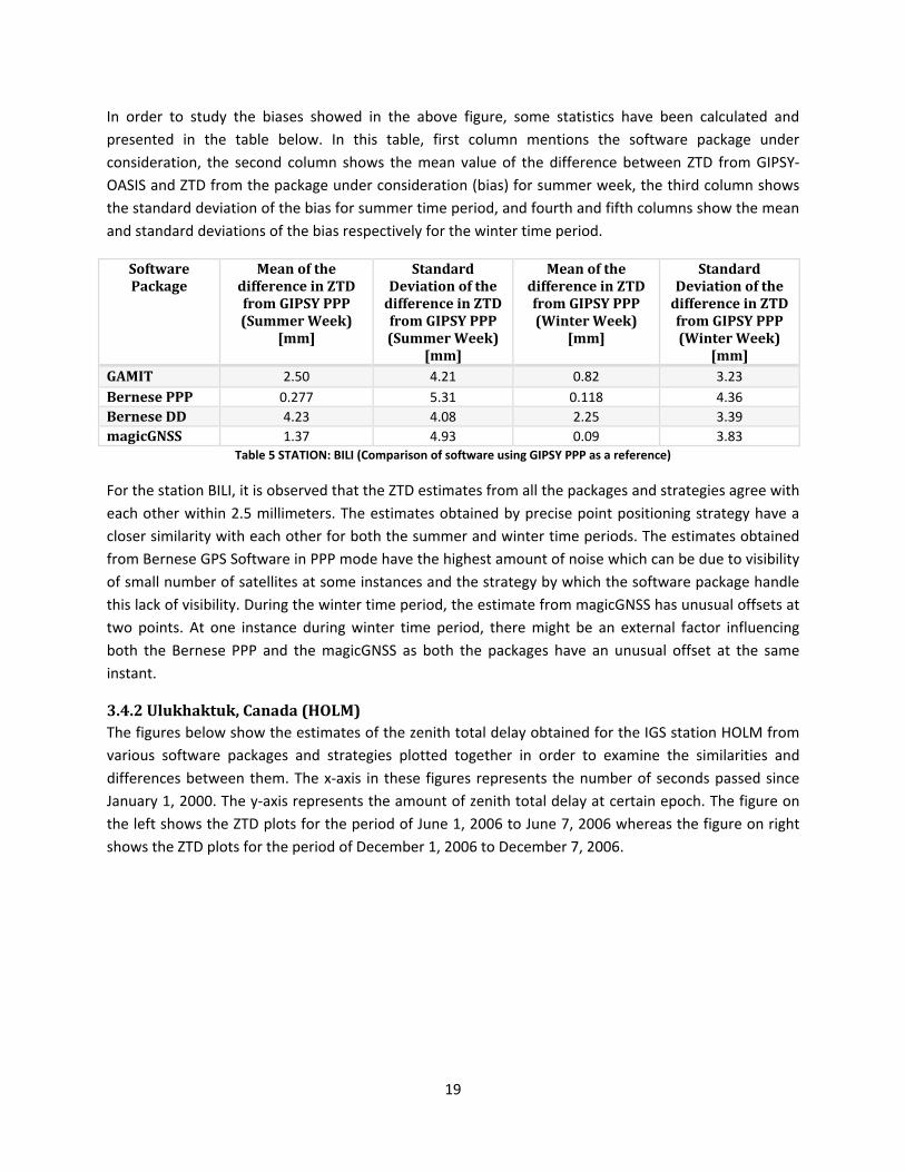
In order to study the biases showed in the above figure, some statistics have been calculated and presented in the table below. In this table, first column mentions the software package under consideration, the second column shows the mean value of the difference between ZTD from GIPSY‐OASIS and ZTD from the package under consideration (bias) for summer week, the third column shows the standard deviation of the bias for summer time period, and fourth and fifth columns show the mean and standard deviations of the bias respectively for the winter time period.
Software Package
Mean of the difference in ZTD from GIPSY PPP (Summer Week)
[mm]
Standard Deviation of the difference in ZTD from GIPSY PPP (Summer Week)
[mm]
Mean of the difference in ZTD from GIPSY PPP (Winter Week)
[mm]
Standard Deviation of the difference in ZTD from GIPSY PPP (Winter Week)
[mm] GAMIT 2.50 4.21 0.82 3.23Bernese PPP 0.277 5.31 0.118 4.36Bernese DD 4.23 4.08 2.25 3.39magicGNSS 1.37 4.93 0.09 3.83
Table 5 STATION: BILI (Comparison of software using GIPSY PPP as a reference)
For the station BILI, it is observed that the ZTD estimates from all the packages and strategies agree with each other within 2.5 millimeters. The estimates obtained by precise point positioning strategy have a closer similarity with each other for both the summer and winter time periods. The estimates obtained from Bernese GPS Software in PPP mode have the highest amount of noise which can be due to visibility of small number of satellites at some instances and the strategy by which the software package handle this lack of visibility. During the winter time period, the estimate from magicGNSS has unusual offsets at two points. At one instance during winter time period, there might be an external factor influencing both the Bernese PPP and the magicGNSS as both the packages have an unusual offset at the same instant.
3.4.2 Ulukhaktuk, Canada (HOLM) The figures below show the estimates of the zenith total delay obtained for the IGS station HOLM from various software packages and strategies plotted together in order to examine the similarities and differences between them. The x‐axis in these figures represents the number of seconds passed since January 1, 2000. The y‐axis represents the amount of zenith total delay at certain epoch. The figure on the left shows the ZTD plots for the period of June 1, 2006 to June 7, 2006 whereas the figure on right shows the ZTD plots for the period of December 1, 2006 to December 7, 2006.
19
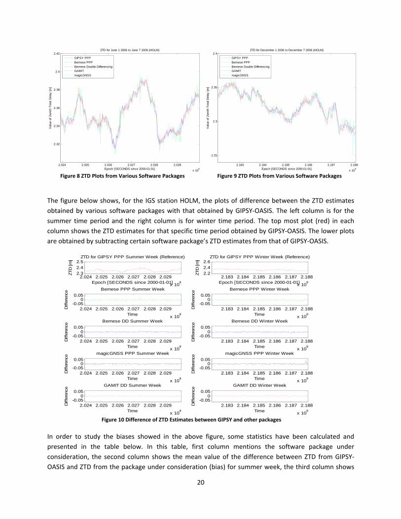
Figure 8 ZTD Plots from Various Software Packages Figure 9 ZTD Plots from Various Software Packages
2.024 2.025 2.026 2.027 2.028 2.029
x 108
2.32
2.34
2.36
2.38
2.4
2.42
Epoch [SECONDS since 2000-01-01]
Val
ue o
f Zen
ith T
otal
Del
ay [m
]ZTD for June 1 2006 to June 7 2006 (HOLM)
GIPSY PPPBernese PPPBernese Double DifferencingGAMITmagicGNSS
2.183 2.184 2.185 2.186 2.187 2.188
x 108
2.25
2.3
2.35
2.4
Epoch [SECONDS since 2000-01-01]
Val
ue o
f Zen
ith T
otal
Del
ay [m
]
ZTD for December 1 2006 to December 7 2006 (HOLM)
GIPSY PPPBernese PPPBernese Double DifferencingGAMITmagicGNSS
The figure below shows, for the IGS station HOLM, the plots of difference between the ZTD estimates obtained by various software packages with that obtained by GIPSY‐OASIS. The left column is for the summer time period and the right column is for winter time period. The top most plot (red) in each column shows the ZTD estimates for that specific time period obtained by GIPSY‐OASIS. The lower plots are obtained by subtracting certain software package’s ZTD estimates from that of GIPSY‐OASIS.
Figure 10 Difference of ZTD Estimates between GIPSY and other packages
2.024 2.025 2.026 2.027 2.028 2.029
x 108
2.32.42.5
ZTD for GIPSY PPP Summer Week (Reference)
Epoch [SECONDS since 2000-01-01]
ZTD
[m]
2.183 2.184 2.185 2.186 2.187 2.188
x 108
2.22.42.6
ZTD for GIPSY PPP Winter Week (Reference)
Epoch [SECONDS since 2000-01-01]
ZTD
[m]
2.183 2.184 2.185 2.186 2.187 2.188
x 108
-0.050
0.05Bernese PPP Winter Week
Time
Diff
eren
ce
2.024 2.025 2.026 2.027 2.028 2.029
x 108
-0.050
0.05Bernese PPP Summer Week
Time
Diff
eren
ce
2.183 2.184 2.185 2.186 2.187 2.188
x 108
-0.050
0.05Bernese DD Winter Week
Time
Diff
eren
ce
2.024 2.025 2.026 2.027 2.028 2.029
x 108
-0.050
0.05Bernese DD Summer Week
Time
Diff
eren
ce
2.024 2.025 2.026 2.027 2.028 2.029
x 108
-0.050
0.05magicGNSS PPP Summer Week
Time
Diff
eren
ce
2.183 2.184 2.185 2.186 2.187 2.188
x 108
-0.050
0.05magicGNSS PPP Winter Week
Time
Diff
eren
ce
2.024 2.025 2.026 2.027 2.028 2.029
x 108
-0.050
0.05GAMIT DD Summer Week
Time
Diff
eren
ce
2.183 2.184 2.185 2.186 2.187 2.188
x 108
-0.050
0.05GAMIT DD Winter Week
Time
Diff
eren
ce
In order to study the biases showed in the above figure, some statistics have been calculated and presented in the table below. In this table, first column mentions the software package under consideration, the second column shows the mean value of the difference between ZTD from GIPSY‐OASIS and ZTD from the package under consideration (bias) for summer week, the third column shows
20
the standard deviation of the bias for summer time period, and fourth and fifth columns show the mean and standard deviations of the bias respectively for the winter time period.
Software Package
Mean of the difference in ZTD from GIPSY PPP (Summer Week)
[mm]
Standard Deviation of the difference in ZTD from GIPSY PPP (Summer Week)
[mm]
Mean of the difference in ZTD from GIPSY PPP (Winter Week)
[mm]
Standard Deviation of the difference in ZTD from GIPSY PPP (Winter Week)
[mm] GAMIT 0.115 2.92 0.093 3.65Bernese PPP ‐1.20 4.90 ‐1.79 4.41Bernese DD ‐0.986 2.92 ‐2.60 3.75magicGNSS 1.60 3.58 1.28 4.23
Table 6 STATION: HOLM (Comparison of software using GIPSY PPP as a reference)
For the station HOLM, it is observed that the ZTD estimates from all the packages and strategies agree with each other within 1.6 millimeters. The estimates obtained from Bernese GPS Software in PPP mode have the highest amount of noise which can be due to visibility of small number of satellites at some instances and the strategy by which the software package handle this lack of visibility. At the end of the winter time period, the estimate from magicGNSS has some unusual big offsets.
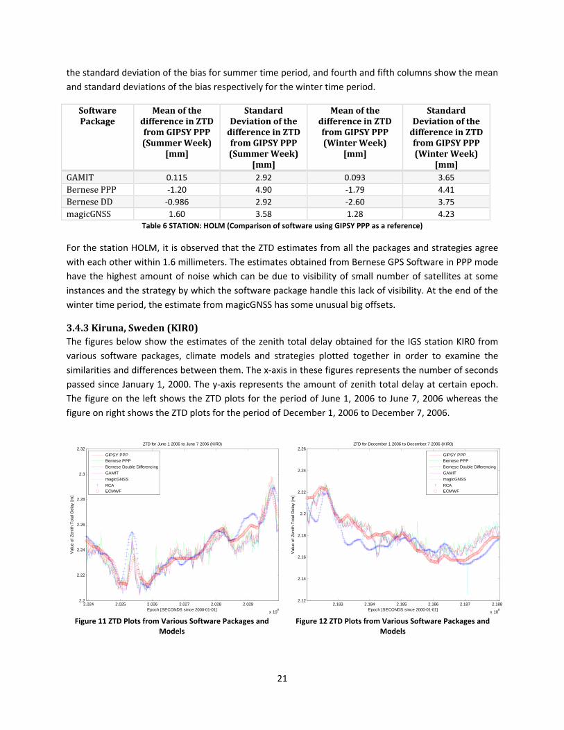
3.4.3 Kiruna, Sweden (KIR0) The figures below show the estimates of the zenith total delay obtained for the IGS station KIR0 from various software packages, climate models and strategies plotted together in order to examine the similarities and differences between them. The x‐axis in these figures represents the number of seconds passed since January 1, 2000. The y‐axis represents the amount of zenith total delay at certain epoch. The figure on the left shows the ZTD plots for the period of June 1, 2006 to June 7, 2006 whereas the figure on right shows the ZTD plots for the period of December 1, 2006 to December 7, 2006.
Figure 11 ZTD Plots from Various Software Packages and
Models
Figure 12 ZTD Plots from Various Software Packages and
Models
2.024 2.025 2.026 2.027 2.028 2.029
x 108
2.2
2.22
2.24
2.26
2.28
2.3
2.32
Epoch [SECONDS since 2000-01-01]
Val
ue o
f Zen
ith T
otal
Del
ay [m
]
ZTD for June 1 2006 to June 7 2006 (KIR0)
GIPSY PPPBernese PPPBernese Double DifferencingGAMITmagicGNSSRCAECMWF
2.183 2.184 2.185 2.186 2.187 2.188
x 108
2.12
2.14
2.16
2.18
2.2
2.22
2.24
2.26
Epoch [SECONDS since 2000-01-01]
Val
ue o
f Zen
ith T
otal
Del
ay [m
]
ZTD for December 1 2006 to December 7 2006 (KIR0)
GIPSY PPPBernese PPPBernese Double DifferencingGAMITmagicGNSSRCAECMWF
21
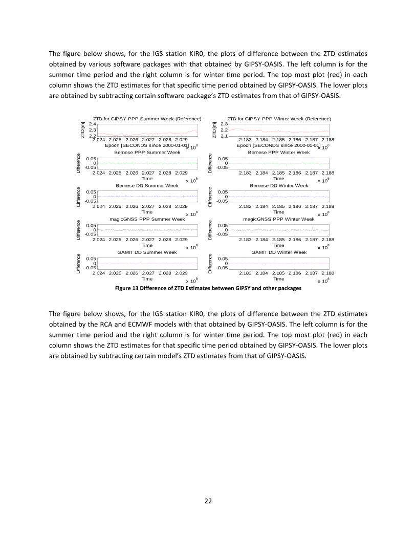
The figure below shows, for the IGS station KIR0, the plots of difference between the ZTD estimates obtained by various software packages with that obtained by GIPSY‐OASIS. The left column is for the summer time period and the right column is for winter time period. The top most plot (red) in each column shows the ZTD estimates for that specific time period obtained by GIPSY‐OASIS. The lower plots are obtained by subtracting certain software package’s ZTD estimates from that of GIPSY‐OASIS.
Figure 13 Difference of ZTD Estimates between GIPSY and other packages
2.024 2.025 2.026 2.027 2.028 2.029
x 108
2.22.32.4
ZTD for GIPSY PPP Summer Week (Reference)
Epoch [SECONDS since 2000-01-01]
ZTD
[m]
2.183 2.184 2.185 2.186 2.187 2.188
x 108
2.12.22.3
ZTD for GIPSY PPP Winter Week (Reference)
Epoch [SECONDS since 2000-01-01]
ZTD
[m]
2.183 2.184 2.185 2.186 2.187 2.188
x 108
-0.050
0.05Bernese PPP Winter Week
Time
Diff
eren
ce
2.024 2.025 2.026 2.027 2.028 2.029
x 108
-0.050
0.05Bernese PPP Summer Week
Time
Diff
eren
ce
2.183 2.184 2.185 2.186 2.187 2.188
x 108
-0.050
0.05Bernese DD Winter Week
TimeD
iffer
ence
2.024 2.025 2.026 2.027 2.028 2.029
x 108
-0.050
0.05Bernese DD Summer Week
Time
Diff
eren
ce
2.024 2.025 2.026 2.027 2.028 2.029
x 108
-0.050
0.05magicGNSS PPP Summer Week
Time
Diff
eren
ce
2.183 2.184 2.185 2.186 2.187 2.188
x 108
-0.050
0.05magicGNSS PPP Winter Week
Time
Diff
eren
ce
2.024 2.025 2.026 2.027 2.028 2.029
x 108
-0.050
0.05GAMIT DD Summer Week
Time
Diff
eren
ce
2.183 2.184 2.185 2.186 2.187 2.188
x 108
-0.050
0.05GAMIT DD Winter Week
Time
Diff
eren
ce
The figure below shows, for the IGS station KIR0, the plots of difference between the ZTD estimates obtained by the RCA and ECMWF models with that obtained by GIPSY‐OASIS. The left column is for the summer time period and the right column is for winter time period. The top most plot (red) in each column shows the ZTD estimates for that specific time period obtained by GIPSY‐OASIS. The lower plots are obtained by subtracting certain model’s ZTD estimates from that of GIPSY‐OASIS.
22

2.024 2.025 2.026 2.027 2.028 2.029
x 108
2.2
2.25
2.3
2.35ZTD for GIPSY PPP Summer Week (Reference)
Epoch [SECONDS since 2000-01-01]ZT
D [m
]2.183 2.184 2.185 2.186 2.187 2.188
x 108
2.1
2.15
2.2
2.25ZTD for GIPSY PPP Winter Week (Reference)
Epoch [SECONDS since 2000-01-01]
ZTD
[m]
2.024 2.025 2.026 2.027 2.028 2.029
x 108
-0.05
0
0.05
RCA
Time
Diff
eren
ce
2.183 2.184 2.185 2.186 2.187 2.188
x 108
-0.05
0
0.05
RCA
Time
Diff
eren
ce2.024 2.025 2.026 2.027 2.028 2.029
x 108
-0.05
0
0.05
ECMWF
Time
Diff
eren
ce
2.183 2.184 2.185 2.186 2.187 2.188
x 108
-0.05
0
0.05
ECMWF
TimeD
iffer
ence
Figure 20 Difference of ZTD Estimates between GIPSY and Climate Models
In order to study the biases showed in the above figure, some statistics have been calculated and presented in the table below. In this table, first column mentions the software package under consideration, the second column shows the mean value of the difference between ZTD from GIPSY‐OASIS and ZTD from the package under consideration (bias) for summer week, the third column shows the standard deviation of the bias for summer time period, and fourth and fifth columns show the mean and standard deviations of the bias respectively for the winter time period.
Software Package
Mean of the difference in ZTD from GIPSY PPP (Summer Week)
[mm]
Standard Deviation of the difference in ZTD from GIPSY PPP (Summer Week)
[mm]
Mean of the difference in ZTD from GIPSY PPP (Winter Week)
[mm]
Standard Deviation of the difference in ZTD from GIPSY PPP (Winter Week)
[mm] GAMIT 1.77 3.14 1.64 2.61Bernese PPP ‐0.18 4.57 ‐1.77 3.83Bernese DD 2.44 3.07 1.14 3.32magicGNSS 0.91 3.47 0.017 4.12
Table 7 STATION: KIR0 (Comparison of software using GIPSY PPP as a reference)
Model Diff. from GIPSY PPP (Summer) [mm] Diff. from GIPSY PPP (Winter) [mm] RCA Mean: ‐3.74, Std. Dev: 9.01 Mean: 6.70, Std. Dev: 8.98 ECMWF Mean: ‐1.25, Std. Dev: 6.06 Mean: 1.86, Std. Dev: 7.08
Table 8 STATION: KIR0 (Comparison of climate models using GIPSY PPP as a reference)
For the station KIR0, it is observed that the RCA and ECMWF models follow the GNSS based estimates. Although there are some disagreements between the two numerical models for both the summer and
23
winter time periods but the GNSS based estimates have a good agreement between each other. ZTD estimates from all the packages and strategies agree with each other within 2.44 millimeters and the models agree with GIPSY PPP estimates within 6.7 millimeters.
The estimates obtained by precise point positioning strategy have a closer similarity with each other. The estimates obtained from Bernese GPS Software in PPP mode have the highest amount of noise which can be due to visibility of small number of satellites at some instances and the strategy by which the software package handle this lack of visibility. During the winter time period, the estimate from magicGNSS has an unusual offsets at one instance.
3.4.4 Ny Alesund, Norway (NYA1) The figures below show the estimates of the zenith total delay obtained for the IGS station NYA1 from various software packages and strategies plotted together in order to examine the similarities and differences between them. The x‐axis in these figures represents the number of seconds passed since January 1, 2000. The y‐axis represents the amount of zenith total delay at certain epoch. The figure on the left shows the ZTD plots for the period of June 1, 2006 to June 7, 2006 whereas the figure on right shows the ZTD plots for the period of December 1, 2006 to December 7, 2006.
Figure 14 ZTD Plots from Various Software Packages
Figure 15 ZTD Plots from Various Software Packages
The figure below shows, for the IGS station NYA1, the plots of difference between the ZTD estimates obtained by various software packages with that obtained by GIPSY‐OASIS. The left column is for the summer time period and the right column is for winter time period. The top most plot (red) in each column shows the ZTD estimates for that specific time period obtained by GIPSY‐OASIS. The lower plots are obtained by subtracting certain software package’s ZTD estimates from that of GIPSY‐OASIS.
2.024 2.025 2.026 2.027 2.028 2.029
x 108
2.31
2.32
2.33
2.34
2.35
2.36
2.37
2.38
Epoch [SECONDS since 2000-01-01]
Val
ue o
f Zen
ith T
otal
Del
ay [m
]
ZTD for June 1 2006 to June 7 2006 (NYA1)
GIPSY PPPBernese PPPBernese Double DifferencingGAMITmagicGNSS
2.183 2.184 2.185 2.186 2.187 2.188
x 108
2.28
2.3
2.32
2.34
2.36
2.38
Epoch [SECONDS since 2000-01-01]
Val
ue o
f Zen
ith T
otal
Del
ay [m
]
ZTD for December 1 2006 to December 7 2006 (NYA1)
GIPSY PPPBernese PPPBernese Double DifferencingGAMITmagicGNSS
24

2.024 2.025 2.026 2.027 2.028 2.029
x 108
2.32.42.5
ZTD for GIPSY PPP Summer Week (Reference)
Epoch [SECONDS since 2000-01-01]
ZTD [m
]
2.183 2.184 2.185 2.186 2.187 2.188
x 108
2.252.3
2.35ZTD for GIPSY PPP Winter Week (Reference)
Epoch [SECONDS since 2000-01-01]
ZTD [m
]
2.183 2.184 2.185 2.186 2.187 2.188
x 108
-0.050
0.05Bernese PPP Winter Week
Time
Diff
eren
ce
2.024 2.025 2.026 2.027 2.028 2.029
x 108
-0.050
0.05Bernese PPP Summer Week
Time
Diff
eren
ce
2.183 2.184 2.185 2.186 2.187 2.188
x 108
-0.050
0.05Bernese DD Winter Week
Time
Diff
eren
ce
2.024 2.025 2.026 2.027 2.028 2.029
x 108
-0.050
0.05Bernese DD Summer Week
Time
Diff
eren
ce
2.024 2.025 2.026 2.027 2.028 2.029
x 108
-0.050
0.05magicGNSS PPP Summer Week
Time
Diff
eren
ce
2.183 2.184 2.185 2.186 2.187 2.188
x 108
-0.050
0.05magicGNSS PPP Winter Week
Time
Diff
eren
ce2.024 2.025 2.026 2.027 2.028 2.029
x 108
-0.050
0.05GAMIT DD Summer Week
Time
Diff
eren
ce
2.183 2.184 2.185 2.186 2.187 2.188
x 108
-0.050
0.05GAMIT DD Winter Week
Time
Diff
eren
ce
Figure 16 Difference of ZTD Estimates between GIPSY and other packages
In order to study the biases showed in the above figure, some statistics have been calculated and presented in the table below. In this table, first column mentions the software package under consideration, the second column shows the mean value of the difference between ZTD from GIPSY‐OASIS and ZTD from the package under consideration (bias) for summer week, the third column shows the standard deviation of the bias for summer time period, and fourth and fifth columns show the mean and standard deviations of the bias respectively for the winter time period.
Software Package
Mean of the difference in ZTD from GIPSY PPP (Summer Week)
[mm]
Standard Deviation of the difference in ZTD from GIPSY PPP (Summer Week)
[mm]
Mean of the difference in ZTD from GIPSY PPP (Winter Week)
[mm]
Standard Deviation of the difference in ZTD from GIPSY PPP (Winter Week)
[mm] GAMIT ‐0.824 2.66 ‐0.002 2.16Bernese PPP ‐2.31 4.16 ‐2.35 5.93Bernese DD ‐0.815 2.94 ‐0.003 2.43magicGNSS ‐0.838 3.65 ‐0.635 3.10
Table 9 STATION: NYA1 (Comparison of software using GIPSY PPP as a reference)
For the station NYA1, it is observed that the ZTD estimates from all the packages and strategies agree with each other within ‐0.002 millimeters. The estimates obtained from Bernese GPS Software in PPP mode have the highest amount of noise which can be due to visibility of small number of satellites at some instances and the strategy by which the software package handle this lack of visibility. At the end of winter time period, the estimate from Bernese PPP has an unusual fluctuation. At some instances
25
during both time periods, there might be an external factor influencing both the Bernese PPP and the magicGNSS as both the packages have an unusual offset near a same instant.
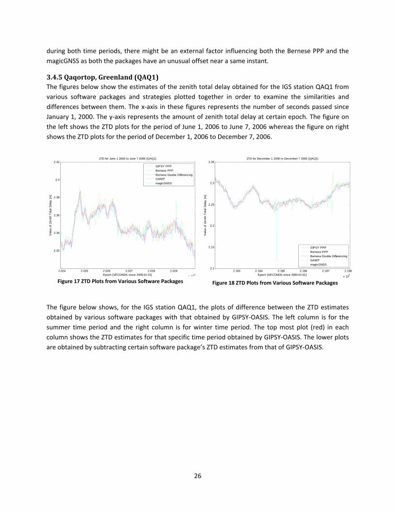
3.4.5 Qaqortop, Greenland (QAQ1) The figures below show the estimates of the zenith total delay obtained for the IGS station QAQ1 from various software packages and strategies plotted together in order to examine the similarities and differences between them. The x‐axis in these figures represents the number of seconds passed since January 1, 2000. The y‐axis represents the amount of zenith total delay at certain epoch. The figure on the left shows the ZTD plots for the period of June 1, 2006 to June 7, 2006 whereas the figure on right shows the ZTD plots for the period of December 1, 2006 to December 7, 2006.
Figure 17 ZTD Plots from Various Software Packages
Figure 18 ZTD Plots from Various Software Packages
The figure below shows, for the IGS station QAQ1, the plots of difference between the ZTD estimates obtained by various software packages with that obtained by GIPSY‐OASIS. The left column is for the summer time period and the right column is for winter time period. The top most plot (red) in each column shows the ZTD estimates for that specific time period obtained by GIPSY‐OASIS. The lower plots are obtained by subtracting certain software package’s ZTD estimates from that of GIPSY‐OASIS.
2.024 2.025 2.026 2.027 2.028 2.029
x 108
2.32
2.34
2.36
2.38
2.4
2.42
Epoch [SECONDS since 2000-01-01]
Val
ue o
f Zen
ith T
otal
Del
ay [m
]
ZTD for June 1 2006 to June 7 2006 (QAQ1)
GIPSY PPPBernese PPPBernese Double DifferencingGAMITmagicGNSS
2.183 2.184 2.185 2.186 2.187 2.188
x 108
2.1
2.15
2.2
2.25
2.3
2.35
Epoch [SECONDS since 2000-01-01]
Val
ue o
f Zen
ith T
otal
Del
ay [m
]
ZTD for December 1 2006 to December 7 2006 (QAQ1)
GIPSY PPPBernese PPPBernese Double DifferencingGAMITmagicGNSS
26
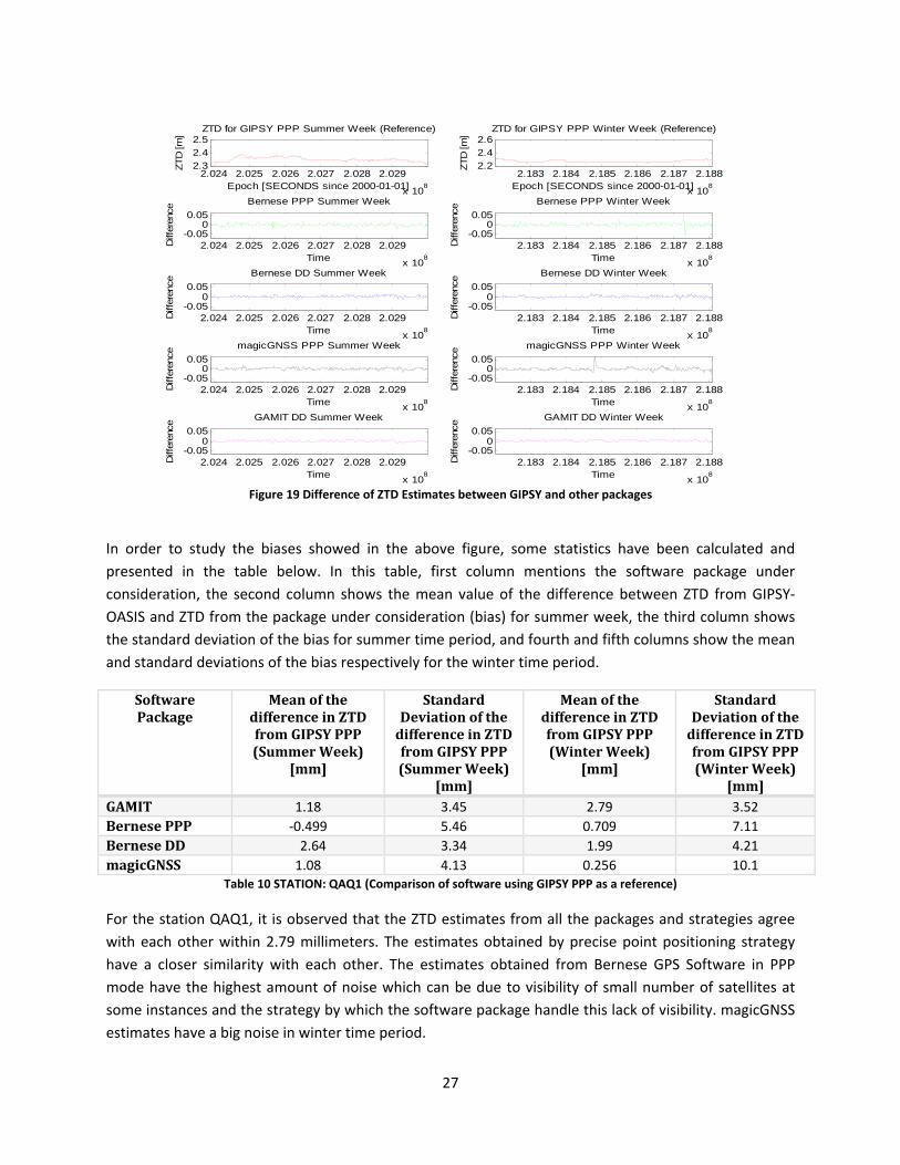
Figure 19 Difference of ZTD Estimates between GIPSY and other packages
2.024 2.025 2.026 2.027 2.028 2.029
x 108
2.32.42.5
ZTD for GIPSY PPP Summer Week (Reference)
Epoch [SECONDS since 2000-01-01]ZT
D [m
]2.183 2.184 2.185 2.186 2.187 2.188
x 108
2.22.42.6
ZTD for GIPSY PPP Winter Week (Reference)
Epoch [SECONDS since 2000-01-01]
ZTD
[m]
2.183 2.184 2.185 2.186 2.187 2.188
x 108
-0.050
0.05Bernese PPP Winter Week
Time
Diff
eren
ce
2.024 2.025 2.026 2.027 2.028 2.029
x 108
-0.050
0.05Bernese PPP Summer Week
Time
Diff
eren
ce
2.183 2.184 2.185 2.186 2.187 2.188
x 108
-0.050
0.05Bernese DD Winter Week
Time
Diff
eren
ce
2.024 2.025 2.026 2.027 2.028 2.029
x 108
-0.050
0.05Bernese DD Summer Week
Time
Diff
eren
ce
2.024 2.025 2.026 2.027 2.028 2.029
x 108
-0.050
0.05magicGNSS PPP Summer Week
Time
Diff
eren
ce
2.183 2.184 2.185 2.186 2.187 2.188
x 108
-0.050
0.05magicGNSS PPP Winter Week
Time
Diff
eren
ce2.024 2.025 2.026 2.027 2.028 2.029
x 108
-0.050
0.05GAMIT DD Summer Week
Time
Diff
eren
ce
2.183 2.184 2.185 2.186 2.187 2.188
x 108
-0.050
0.05GAMIT DD Winter Week
Time
Diff
eren
ce
In order to study the biases showed in the above figure, some statistics have been calculated and presented in the table below. In this table, first column mentions the software package under consideration, the second column shows the mean value of the difference between ZTD from GIPSY‐OASIS and ZTD from the package under consideration (bias) for summer week, the third column shows the standard deviation of the bias for summer time period, and fourth and fifth columns show the mean and standard deviations of the bias respectively for the winter time period.
Software Package
Mean of the difference in ZTD from GIPSY PPP (Summer Week)
[mm]
Standard Deviation of the difference in ZTD from GIPSY PPP (Summer Week)
[mm]
Mean of the difference in ZTD from GIPSY PPP (Winter Week)
[mm]
Standard Deviation of the difference in ZTD from GIPSY PPP (Winter Week)
[mm] GAMIT 1.18 3.45 2.79 3.52Bernese PPP ‐0.499 5.46 0.709 7.11Bernese DD 2.64 3.34 1.99 4.21magicGNSS 1.08 4.13 0.256 10.1
Table 10 STATION: QAQ1 (Comparison of software using GIPSY PPP as a reference)
27
For the station QAQ1, it is observed that the ZTD estimates from all the packages and strategies agree with each other within 2.79 millimeters. The estimates obtained by precise point positioning strategy have a closer similarity with each other. The estimates obtained from Bernese GPS Software in PPP mode have the highest amount of noise which can be due to visibility of small number of satellites at some instances and the strategy by which the software package handle this lack of visibility. magicGNSS estimates have a big noise in winter time period.
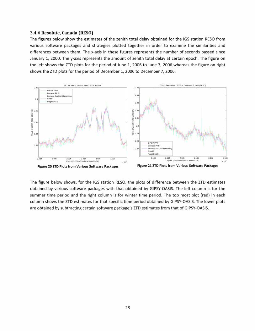
3.4.6 Resolute, Canada (RESO) The figures below show the estimates of the zenith total delay obtained for the IGS station RESO from various software packages and strategies plotted together in order to examine the similarities and differences between them. The x‐axis in these figures represents the number of seconds passed since January 1, 2000. The y‐axis represents the amount of zenith total delay at certain epoch. The figure on the left shows the ZTD plots for the period of June 1, 2006 to June 7, 2006 whereas the figure on right shows the ZTD plots for the period of December 1, 2006 to December 7, 2006.
Figure 20 ZTD Plots from Various Software Packages Figure 21 ZTD Plots from Various Software Packages
The figure below shows, for the IGS station RESO, the plots of difference between the ZTD estimates obtained by various software packages with that obtained by GIPSY‐OASIS. The left column is for the summer time period and the right column is for winter time period. The top most plot (red) in each column shows the ZTD estimates for that specific time period obtained by GIPSY‐OASIS. The lower plots are obtained by subtracting certain software package’s ZTD estimates from that of GIPSY‐OASIS.
2.024 2.025 2.026 2.027 2.028 2.029
x 108
2.32
2.34
2.36
2.38
2.4
2.42
Epoch [SECONDS since 2000-01-01]
Val
ue o
f Zen
ith T
otal
Del
ay [m
]
ZTD for June 1 2006 to June 7 2006 (RESO)
GIPSY PPPBernese PPPBernese Double DifferencingGAMITmagicGNSS
2.183 2.184 2.185 2.186 2.187 2.188
x 108
2.27
2.28
2.29
2.3
2.31
2.32
2.33
2.34
2.35
Epoch [SECONDS since 2000-01-01]
Val
ue o
f Zen
ith T
otal
Del
ay [m
]
ZTD for December 1 2006 to December 7 2006 (RESO)
GIPSY PPPBernese PPPBernese Double DifferencingGAMITmagicGNSS
28
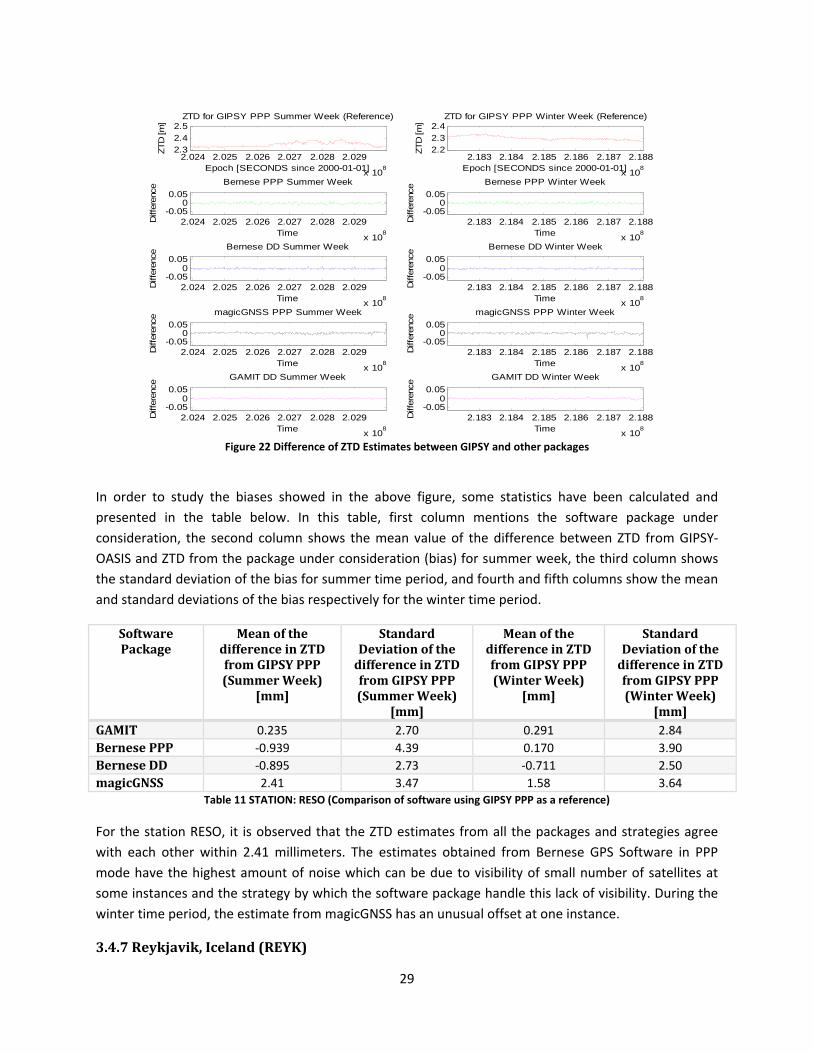
Figure 22 Difference of ZTD Estimates between GIPSY and other packages
2.024 2.025 2.026 2.027 2.028 2.029
x 108
2.32.42.5
ZTD for GIPSY PPP Summer Week (Reference)
Epoch [SECONDS since 2000-01-01]ZT
D [m
]2.183 2.184 2.185 2.186 2.187 2.188
x 108
2.22.32.4
ZTD for GIPSY PPP Winter Week (Reference)
Epoch [SECONDS since 2000-01-01]
ZTD
[m]
2.183 2.184 2.185 2.186 2.187 2.188
x 108
-0.050
0.05Bernese PPP Winter Week
Time
Diff
eren
ce
2.024 2.025 2.026 2.027 2.028 2.029
x 108
-0.050
0.05Bernese PPP Summer Week
Time
Diff
eren
ce
2.183 2.184 2.185 2.186 2.187 2.188
x 108
-0.050
0.05Bernese DD Winter Week
Time
Diff
eren
ce
2.024 2.025 2.026 2.027 2.028 2.029
x 108
-0.050
0.05Bernese DD Summer Week
Time
Diff
eren
ce
2.024 2.025 2.026 2.027 2.028 2.029
x 108
-0.050
0.05magicGNSS PPP Summer Week
Time
Diff
eren
ce
2.183 2.184 2.185 2.186 2.187 2.188
x 108
-0.050
0.05magicGNSS PPP Winter Week
Time
Diff
eren
ce2.024 2.025 2.026 2.027 2.028 2.029
x 108
-0.050
0.05GAMIT DD Summer Week
Time
Diff
eren
ce
2.183 2.184 2.185 2.186 2.187 2.188
x 108
-0.050
0.05GAMIT DD Winter Week
Time
Diff
eren
ce
In order to study the biases showed in the above figure, some statistics have been calculated and presented in the table below. In this table, first column mentions the software package under consideration, the second column shows the mean value of the difference between ZTD from GIPSY‐OASIS and ZTD from the package under consideration (bias) for summer week, the third column shows the standard deviation of the bias for summer time period, and fourth and fifth columns show the mean and standard deviations of the bias respectively for the winter time period.
Software Package
Mean of the difference in ZTD from GIPSY PPP (Summer Week)
[mm]
Standard Deviation of the difference in ZTD from GIPSY PPP (Summer Week)
[mm]
Mean of the difference in ZTD from GIPSY PPP (Winter Week)
[mm]
Standard Deviation of the difference in ZTD from GIPSY PPP (Winter Week)
[mm] GAMIT 0.235 2.70 0.291 2.84Bernese PPP ‐0.939 4.39 0.170 3.90Bernese DD ‐0.895 2.73 ‐0.711 2.50magicGNSS 2.41 3.47 1.58 3.64
Table 11 STATION: RESO (Comparison of software using GIPSY PPP as a reference)
For the station RESO, it is observed that the ZTD estimates from all the packages and strategies agree with each other within 2.41 millimeters. The estimates obtained from Bernese GPS Software in PPP mode have the highest amount of noise which can be due to visibility of small number of satellites at some instances and the strategy by which the software package handle this lack of visibility. During the winter time period, the estimate from magicGNSS has an unusual offset at one instance.
3.4.7 Reykjavik, Iceland (REYK)
29
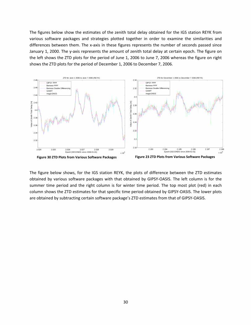
The figures below show the estimates of the zenith total delay obtained for the IGS station REYK from various software packages and strategies plotted together in order to examine the similarities and differences between them. The x‐axis in these figures represents the number of seconds passed since January 1, 2000. The y‐axis represents the amount of zenith total delay at certain epoch. The figure on the left shows the ZTD plots for the period of June 1, 2006 to June 7, 2006 whereas the figure on right shows the ZTD plots for the period of December 1, 2006 to December 7, 2006.
Figure 30 ZTD Plots from Various Software Packages Figure 23 ZTD Plots from Various Software Packages
The figure below shows, for the IGS station REYK, the plots of difference between the ZTD estimates obtained by various software packages with that obtained by GIPSY‐OASIS. The left column is for the summer time period and the right column is for winter time period. The top most plot (red) in each column shows the ZTD estimates for that specific time period obtained by GIPSY‐OASIS. The lower plots are obtained by subtracting certain software package’s ZTD estimates from that of GIPSY‐OASIS.
2.024 2.025 2.026 2.027 2.028 2.029
x 108
2.32
2.34
2.36
2.38
2.4
2.42
2.44
2.46
2.48
Epoch [SECONDS since 2000-01-01]
Val
ue o
f Zen
ith T
otal
Del
ay [m
]
ZTD for June 1 2006 to June 7 2006 (REYK)
GIPSY PPPBernese PPPBernese Double DifferencingGAMITmagicGNSS
2.183 2.184 2.185 2.186 2.187 2.188
x 108
2.18
2.2
2.22
2.24
2.26
2.28
2.3
2.32
2.34
Epoch [SECONDS since 2000-01-01]
Val
ue o
f Zen
ith T
otal
Del
ay [m
]
ZTD for December 1 2006 to December 7 2006 (REYK)
GIPSY PPPBernese PPPBernese Double DifferencingGAMITmagicGNSS
30

Figure 24 Difference of ZTD Estimates between GIPSY and other packages
2.024 2.025 2.026 2.027 2.028 2.029
x 108
2.22.42.6
ZTD for GIPSY PPP Summer Week (Reference)
Epoch [SECONDS since 2000-01-01]ZT
D [m
]2.183 2.184 2.185 2.186 2.187 2.188
x 108
2.22.42.6
ZTD for GIPSY PPP Winter Week (Reference)
Epoch [SECONDS since 2000-01-01]
ZTD
[m]
2.183 2.184 2.185 2.186 2.187 2.188
x 108
-0.050
0.05Bernese PPP Winter Week
Time
Diff
eren
ce
2.024 2.025 2.026 2.027 2.028 2.029
x 108
-0.050
0.05Bernese PPP Summer Week
Time
Diff
eren
ce
2.183 2.184 2.185 2.186 2.187 2.188
x 108
-0.050
0.05Bernese DD Winter Week
Time
Diff
eren
ce
2.024 2.025 2.026 2.027 2.028 2.029
x 108
-0.050
0.05Bernese DD Summer Week
Time
Diff
eren
ce
2.024 2.025 2.026 2.027 2.028 2.029
x 108
-0.050
0.05magicGNSS PPP Summer Week
Time
Diff
eren
ce
2.183 2.184 2.185 2.186 2.187 2.188
x 108
-0.050
0.05magicGNSS PPP Winter Week
Time
Diff
eren
ce2.024 2.025 2.026 2.027 2.028 2.029
x 108
-0.050
0.05GAMIT DD Summer Week
Time
Diff
eren
ce
2.183 2.184 2.185 2.186 2.187 2.188
x 108
-0.050
0.05GAMIT DD Winter Week
Time
Diff
eren
ce
In order to study the biases showed in the above figure, some statistics have been calculated and presented in the table below. In this table, first column mentions the software package under consideration, the second column shows the mean value of the difference between ZTD from GIPSY‐OASIS and ZTD from the package under consideration (bias) for summer week, the third column shows the standard deviation of the bias for summer time period, and fourth and fifth columns show the mean and standard deviations of the bias respectively for the winter time period.
Software Package
Mean of the difference in ZTD from GIPSY PPP (Summer Week)
[mm]
Standard Deviation of the difference in ZTD from GIPSY PPP (Summer Week)
[mm]
Mean of the difference in ZTD from GIPSY PPP (Winter Week)
[mm]
Standard Deviation of the difference in ZTD from GIPSY PPP (Winter Week)
[mm] GAMIT 1.65 3.20 2.51 3.78Bernese PPP 1.20 4.80 0.35 6.11Bernese DD 4.31 3.85 3.24 4.22magicGNSS 0.64 4.92 ‐0.0918 5.77
Table 12 STATION: REYK (Comparison of software using GIPSY PPP as a reference)
For the station REYK, it is observed that the ZTD estimates from all the packages and strategies agree with each other within 4.31 millimeters. The estimates obtained by precise point positioning strategy have a closer similarity with each other. The estimates obtained from Bernese GPS Software in PPP mode have the highest amount of noise which can be due to visibility of small number of satellites at some instances and the strategy by which the software package handle this lack of visibility.
3.4.8 Scoresbysund, Greenland (SCOR)
31
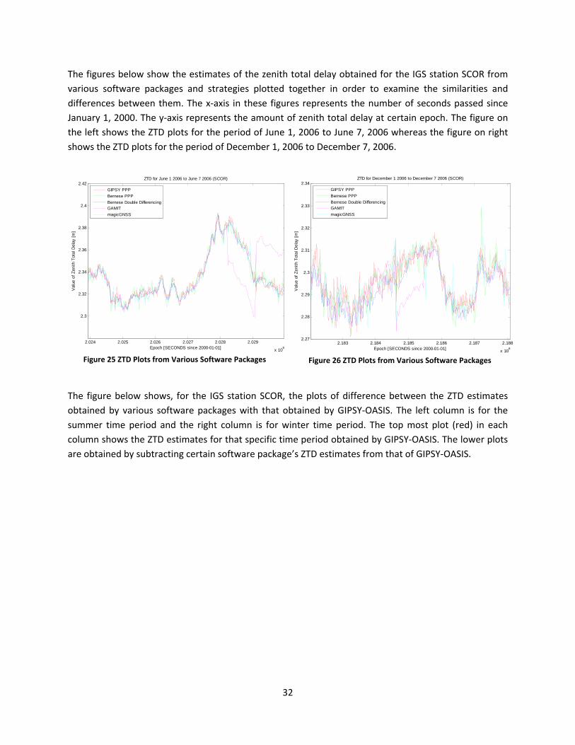
The figures below show the estimates of the zenith total delay obtained for the IGS station SCOR from various software packages and strategies plotted together in order to examine the similarities and differences between them. The x‐axis in these figures represents the number of seconds passed since January 1, 2000. The y‐axis represents the amount of zenith total delay at certain epoch. The figure on the left shows the ZTD plots for the period of June 1, 2006 to June 7, 2006 whereas the figure on right shows the ZTD plots for the period of December 1, 2006 to December 7, 2006.
Figure 25 ZTD Plots from Various Software Packages Figure 26 ZTD Plots from Various Software Packages
The figure below shows, for the IGS station SCOR, the plots of difference between the ZTD estimates obtained by various software packages with that obtained by GIPSY‐OASIS. The left column is for the summer time period and the right column is for winter time period. The top most plot (red) in each column shows the ZTD estimates for that specific time period obtained by GIPSY‐OASIS. The lower plots are obtained by subtracting certain software package’s ZTD estimates from that of GIPSY‐OASIS.
2.024 2.025 2.026 2.027 2.028 2.029
x 108
2.3
2.32
2.34
2.36
2.38
2.4
2.42
Epoch [SECONDS since 2000-01-01]
Val
ue o
f Zen
ith T
otal
Del
ay [m
]
ZTD for June 1 2006 to June 7 2006 (SCOR)
GIPSY PPPBernese PPPBernese Double DifferencingGAMITmagicGNSS
2.183 2.184 2.185 2.186 2.187 2.188
x 108
2.27
2.28
2.29
2.3
2.31
2.32
2.33
2.34
Epoch [SECONDS since 2000-01-01]
Val
ue o
f Zen
ith T
otal
Del
ay [m
]
ZTD for December 1 2006 to December 7 2006 (SCOR)
GIPSY PPPBernese PPPBernese Double DifferencingGAMITmagicGNSS
32

Figure 27 Difference of ZTD Estimates between GIPSY and other packages
2.024 2.025 2.026 2.027 2.028 2.029
x 108
2.32.42.5
ZTD for GIPSY PPP Summer Week (Reference)
Epoch [SECONDS since 2000-01-01]ZT
D [m
]2.183 2.184 2.185 2.186 2.187 2.188
x 108
2.22.32.4
ZTD for GIPSY PPP Winter Week (Reference)
Epoch [SECONDS since 2000-01-01]
ZTD
[m]
2.183 2.184 2.185 2.186 2.187 2.188
x 108
-0.050
0.05Bernese PPP Winter Week
Time
Diff
eren
ce
2.024 2.025 2.026 2.027 2.028 2.029
x 108
-0.050
0.05Bernese PPP Summer Week
Time
Diff
eren
ce
2.183 2.184 2.185 2.186 2.187 2.188
x 108
-0.050
0.05Bernese DD Winter Week
Time
Diff
eren
ce
2.024 2.025 2.026 2.027 2.028 2.029
x 108
-0.050
0.05Bernese DD Summer Week
Time
Diff
eren
ce
2.024 2.025 2.026 2.027 2.028 2.029
x 108
-0.050
0.05magicGNSS PPP Summer Week
Time
Diff
eren
ce
2.183 2.184 2.185 2.186 2.187 2.188
x 108
-0.050
0.05magicGNSS PPP Winter Week
Time
Diff
eren
ce2.024 2.025 2.026 2.027 2.028 2.029
x 108
-0.050
0.05GAMIT DD Summer Week
Time
Diff
eren
ce
2.183 2.184 2.185 2.186 2.187 2.188
x 108
-0.050
0.05GAMIT DD Winter Week
Time
Diff
eren
ce
In order to study the biases showed in the above figure, some statistics have been calculated and presented in the table below. In this table, first column mentions the software package under consideration, the second column shows the mean value of the difference between ZTD from GIPSY‐OASIS and ZTD from the package under consideration (bias) for summer week, the third column shows the standard deviation of the bias for summer time period, and fourth and fifth columns show the mean and standard deviations of the bias respectively for the winter time period.
Software Package
Mean of the difference in ZTD from GIPSY PPP (Summer Week)
[mm]
Standard Deviation of the difference in
ZTD from GIPSY PPP (Summer Week) [mm]
Mean of the difference in ZTD from GIPSY PPP
(Winter Week) [mm]
Standard Deviation of the difference in ZTD from GIPSY PPP (Winter Week)
[mm] GAMIT 1.34 19.04 4.14 6.99Bernese PPP 0.963 4.76 1.36 5.00Bernese DD 1.70 2.88 2.84 4.48magicGNSS 1.49 3.47 0.295 4.91
Table 13 STATION: SCOR (Comparison of software using GIPSY PPP as a reference)
For the station SCOR, it is observed that the ZTD estimates from all the packages and strategies agree with each other within 4.14 millimeters. The estimates obtained from GAMIT GPS Processing Software have the highest standard deviation due to a visible offset in both summer as well as winter time period. These offsets have a length of 24 hours and they are most probably introduced due to a human error. The Bernese PPP estimates are again seen to have relatively more fluctuations. For this station, the measurements from winter time period are more noisy.
33

3.4.9 Thule Airbase, Greenland (THU2) The figures below show the estimates of the zenith total delay obtained for the IGS station THU2 from various software packages and strategies plotted together in order to examine the similarities and differences between them. The x‐axis in these figures represents the number of seconds passed since January 1, 2000. The y‐axis represents the amount of zenith total delay at certain epoch. The figure on the left shows the ZTD plots for the period of June 1, 2006 to June 7, 2006 whereas the figure on right shows the ZTD plots for the period of December 1, 2006 to December 7, 2006.
Figure 28 ZTD Plots from Various Software Packages Figure 29 ZTD Plots from Various Software Packages
The figure below shows, for the IGS station THU2, the plots of difference between the ZTD estimates obtained by various software packages with that obtained by GIPSY‐OASIS. The left column is for the summer time period and the right column is for winter time period. The top most plot (red) in each column shows the ZTD estimates for that specific time period obtained by GIPSY‐OASIS. The lower plots are obtained by subtracting certain software package’s ZTD estimates from that of GIPSY‐OASIS.
2.024 2.025 2.026 2.027 2.028 2.029
x 108
2.31
2.32
2.33
2.34
2.35
2.36
2.37
2.38
2.39
2.4
Epoch [SECONDS since 2000-01-01]
Val
ue o
f Zen
ith T
otal
Del
ay [m
]
ZTD for June 1 2006 to June 7 2006 (THU2)
GIPSY PPPBernese PPPBernese Double DifferencingGAMITmagicGNSS
2.183 2.184 2.185 2.186 2.187 2.188
x 108
2.25
2.26
2.27
2.28
2.29
2.3
2.31
2.32
Epoch [SECONDS since 2000-01-01]
Val
ue o
f Zen
ith T
otal
Del
ay [m
]
ZTD for December 1 2006 to December 7 2006 (THU2)
GIPSY PPPBernese PPPBernese Double DifferencingGAMITmagicGNSS
34
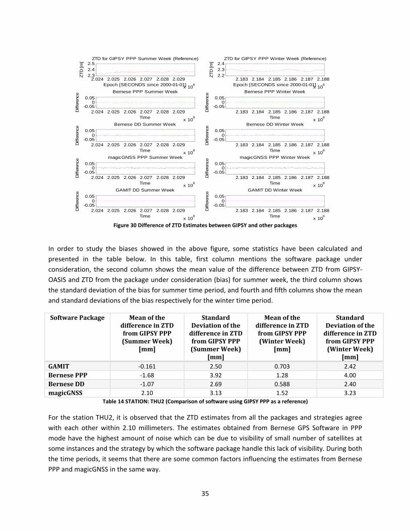
Figure 30 Difference of ZTD Estimates between GIPSY and other packages
2.024 2.025 2.026 2.027 2.028 2.029
x 108
2.32.42.5
ZTD for GIPSY PPP Summer Week (Reference)
Epoch [SECONDS since 2000-01-01]ZT
D [m
]2.183 2.184 2.185 2.186 2.187 2.188
x 108
2.22.32.4
ZTD for GIPSY PPP Winter Week (Reference)
Epoch [SECONDS since 2000-01-01]
ZTD
[m]
2.183 2.184 2.185 2.186 2.187 2.188
x 108
-0.050
0.05Bernese PPP Winter Week
Time
Diff
eren
ce
2.024 2.025 2.026 2.027 2.028 2.029
x 108
-0.050
0.05Bernese PPP Summer Week
Time
Diff
eren
ce
2.183 2.184 2.185 2.186 2.187 2.188
x 108
-0.050
0.05Bernese DD Winter Week
Time
Diff
eren
ce
2.024 2.025 2.026 2.027 2.028 2.029
x 108
-0.050
0.05Bernese DD Summer Week
Time
Diff
eren
ce
2.024 2.025 2.026 2.027 2.028 2.029
x 108
-0.050
0.05magicGNSS PPP Summer Week
Time
Diff
eren
ce
2.183 2.184 2.185 2.186 2.187 2.188
x 108
-0.050
0.05magicGNSS PPP Winter Week
Time
Diff
eren
ce2.024 2.025 2.026 2.027 2.028 2.029
x 108
-0.050
0.05GAMIT DD Summer Week
Time
Diff
eren
ce
2.183 2.184 2.185 2.186 2.187 2.188
x 108
-0.050
0.05GAMIT DD Winter Week
Time
Diff
eren
ce
In order to study the biases showed in the above figure, some statistics have been calculated and presented in the table below. In this table, first column mentions the software package under consideration, the second column shows the mean value of the difference between ZTD from GIPSY‐OASIS and ZTD from the package under consideration (bias) for summer week, the third column shows the standard deviation of the bias for summer time period, and fourth and fifth columns show the mean and standard deviations of the bias respectively for the winter time period.
Software Package Mean of the difference in ZTD from GIPSY PPP (Summer Week)
[mm]
Standard Deviation of the difference in ZTD from GIPSY PPP (Summer Week)
[mm]
Mean of the difference in ZTD from GIPSY PPP (Winter Week)
[mm]
Standard Deviation of the difference in ZTD from GIPSY PPP (Winter Week)
[mm] GAMIT ‐0.161 2.50 0.703 2.42Bernese PPP ‐1.68 3.92 1.28 4.00Bernese DD ‐1.07 2.69 0.588 2.40magicGNSS 2.10 3.13 1.52 3.23
Table 14 STATION: THU2 (Comparison of software using GIPSY PPP as a reference)
For the station THU2, it is observed that the ZTD estimates from all the packages and strategies agree with each other within 2.10 millimeters. The estimates obtained from Bernese GPS Software in PPP mode have the highest amount of noise which can be due to visibility of small number of satellites at some instances and the strategy by which the software package handle this lack of visibility. During both the time periods, it seems that there are some common factors influencing the estimates from Bernese PPP and magicGNSS in the same way.
35

3.4.10 Thule Airbase, Greenland (THU3) The figures below show the estimates of the zenith total delay obtained for the IGS station THU3 from various software packages and strategies plotted together in order to examine the similarities and differences between them. The x‐axis in these figures represents the number of seconds passed since January 1, 2000. The y‐axis represents the amount of zenith total delay at certain epoch. The figure on the left shows the ZTD plots for the period of June 1, 2006 to June 7, 2006 whereas the figure on right shows the ZTD plots for the period of December 1, 2006 to December 7, 2006.
Figure 31 ZTD Plots from Various Software Packages
Figure 40 ZTD Plots from Various Software Packages
The figure below shows, for the IGS station THU3, the plots of difference between the ZTD estimates obtained by various software packages with that obtained by GIPSY‐OASIS. The left column is for the summer time period and the right column is for winter time period. The top most plot (red) in each column shows the ZTD estimates for that specific time period obtained by GIPSY‐OASIS. The lower plots are obtained by subtracting certain software package’s ZTD estimates from that of GIPSY‐OASIS.
2.024 2.025 2.026 2.027 2.028 2.029
x 108
2.31
2.32
2.33
2.34
2.35
2.36
2.37
2.38
2.39
2.4
Epoch [SECONDS since 2000-01-01]
Val
ue o
f Zen
ith T
otal
Del
ay [m
]
ZTD for June 1 2006 to June 7 2006 (THU3)
GIPSY PPPBernese PPPBernese Double DifferencingGAMITmagicGNSS
2.183 2.184 2.185 2.186 2.187 2.188
x 108
2.25
2.26
2.27
2.28
2.29
2.3
2.31
2.32
Epoch [SECONDS since 2000-01-01]
Val
ue o
f Zen
ith T
otal
Del
ay [m
]
ZTD for December 1 2006 to December 7 2006 (THU3)
GIPSY PPPBernese PPPBernese Double DifferencingGAMITmagicGNSS
36
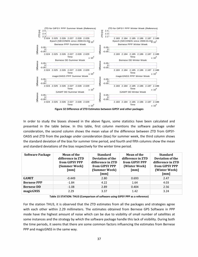
Figure 32 Difference of ZTD Estimates between GIPSY and other packages
2.024 2.025 2.026 2.027 2.028 2.029
x 108
2.32.42.5
ZTD for GIPSY PPP Summer Week (Reference)
Epoch [SECONDS since 2000-01-01]ZT
D [m
]2.183 2.184 2.185 2.186 2.187 2.188
x 108
2.22.32.4
ZTD for GIPSY PPP Winter Week (Reference)
Epoch [SECONDS since 2000-01-01]
ZTD
[m]
2.183 2.184 2.185 2.186 2.187 2.188
x 108
-0.050
0.05Bernese PPP Winter Week
Time
Diff
eren
ce
2.024 2.025 2.026 2.027 2.028 2.029
x 108
-0.050
0.05Bernese PPP Summer Week
Time
Diff
eren
ce
2.183 2.184 2.185 2.186 2.187 2.188
x 108
-0.050
0.05Bernese DD Winter Week
Time
Diff
eren
ce
2.024 2.025 2.026 2.027 2.028 2.029
x 108
-0.050
0.05Bernese DD Summer Week
Time
Diff
eren
ce
2.024 2.025 2.026 2.027 2.028 2.029
x 108
-0.050
0.05magicGNSS PPP Summer Week
Time
Diff
eren
ce
2.183 2.184 2.185 2.186 2.187 2.188
x 108
-0.050
0.05magicGNSS PPP Winter Week
Time
Diff
eren
ce2.024 2.025 2.026 2.027 2.028 2.029
x 108
-0.050
0.05GAMIT DD Summer Week
Time
Diff
eren
ce
2.183 2.184 2.185 2.186 2.187 2.188
x 108
-0.050
0.05GAMIT DD Winter Week
Time
Diff
eren
ce
In order to study the biases showed in the above figure, some statistics have been calculated and presented in the table below. In this table, first column mentions the software package under consideration, the second column shows the mean value of the difference between ZTD from GIPSY‐OASIS and ZTD from the package under consideration (bias) for summer week, the third column shows the standard deviation of the bias for summer time period, and fourth and fifth columns show the mean and standard deviations of the bias respectively for the winter time period.
Software Package Mean of the difference in ZTD from GIPSY PPP (Summer Week)
[mm]
Standard Deviation of the difference in ZTD from GIPSY PPP (Summer Week)
[mm]
Mean of the difference in ZTD from GIPSY PPP (Winter Week)
[mm]
Standard Deviation of the difference in ZTD from GIPSY PPP (Winter Week)
[mm] GAMIT ‐0.449 2.80 0.693 2.47Bernese PPP ‐1.84 4.22 1.64 4.03Bernese DD ‐1.08 2.89 0.404 2.56magicGNSS 2.29 3.37 1.42 3.24
Table 15 STATION: THU3 (Comparison of software using GIPSY PPP as a reference)
For the station THU3, it is observed that the ZTD estimates from all the packages and strategies agree with each other within 2.29 millimeters. The estimates obtained from Bernese GPS Software in PPP mode have the highest amount of noise which can be due to visibility of small number of satellites at some instances and the strategy by which the software package handle this lack of visibility. During both the time periods, it seems that there are some common factors influencing the estimates from Bernese PPP and magicGNSS in the same way.
37
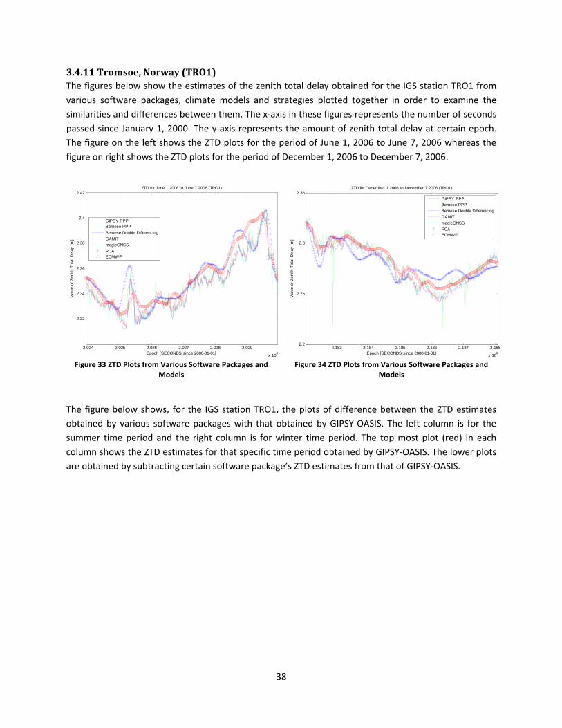
3.4.11 Tromsoe, Norway (TRO1) The figures below show the estimates of the zenith total delay obtained for the IGS station TRO1 from various software packages, climate models and strategies plotted together in order to examine the similarities and differences between them. The x‐axis in these figures represents the number of seconds passed since January 1, 2000. The y‐axis represents the amount of zenith total delay at certain epoch. The figure on the left shows the ZTD plots for the period of June 1, 2006 to June 7, 2006 whereas the figure on right shows the ZTD plots for the period of December 1, 2006 to December 7, 2006.
Figure 33 ZTD Plots from Various Software Packages and
Models
Figure 34 ZTD Plots from Various Software Packages and
Models
The figure below shows, for the IGS station TRO1, the plots of difference between the ZTD estimates obtained by various software packages with that obtained by GIPSY‐OASIS. The left column is for the summer time period and the right column is for winter time period. The top most plot (red) in each column shows the ZTD estimates for that specific time period obtained by GIPSY‐OASIS. The lower plots are obtained by subtracting certain software package’s ZTD estimates from that of GIPSY‐OASIS.
2.024 2.025 2.026 2.027 2.028 2.029
x 108
2.32
2.34
2.36
2.38
2.4
2.42
Epoch [SECONDS since 2000-01-01]
Val
ue o
f Zen
ith T
otal
Del
ay [m
]
ZTD for June 1 2006 to June 7 2006 (TRO1)
GIPSY PPPBernese PPPBernese Double DifferencingGAMITmagicGNSSRCAECMWF
2.183 2.184 2.185 2.186 2.187 2.188
x 108
2.2
2.25
2.3
2.35
Epoch [SECONDS since 2000-01-01]
Val
ue o
f Zen
ith T
otal
Del
ay [m
]
ZTD for December 1 2006 to December 7 2006 (TRO1)
GIPSY PPPBernese PPPBernese Double DifferencingGAMITmagicGNSSRCAECMWF
38

Figure 35 Difference of ZTD Estimates between GIPSY and other packages
2.024 2.025 2.026 2.027 2.028 2.029
x 108
2.22.42.6
ZTD for GIPSY PPP Summer Week (Reference)
Epoch [SECONDS since 2000-01-01]ZT
D [m
]2.183 2.184 2.185 2.186 2.187 2.188
x 108
2.22.42.6
ZTD for GIPSY PPP Winter Week (Reference)
Epoch [SECONDS since 2000-01-01]
ZTD
[m]
2.183 2.184 2.185 2.186 2.187 2.188
x 108
-0.050
0.05Bernese PPP Winter Week
Time
Diff
eren
ce
2.024 2.025 2.026 2.027 2.028 2.029
x 108
-0.050
0.05Bernese PPP Summer Week
Time
Diff
eren
ce
2.183 2.184 2.185 2.186 2.187 2.188
x 108
-0.050
0.05Bernese DD Winter Week
Time
Diff
eren
ce
2.024 2.025 2.026 2.027 2.028 2.029
x 108
-0.050
0.05Bernese DD Summer Week
Time
Diff
eren
ce
2.024 2.025 2.026 2.027 2.028 2.029
x 108
-0.050
0.05magicGNSS PPP Summer Week
Time
Diff
eren
ce
2.183 2.184 2.185 2.186 2.187 2.188
x 108
-0.050
0.05magicGNSS PPP Winter Week
Time
Diff
eren
ce2.024 2.025 2.026 2.027 2.028 2.029
x 108
-0.050
0.05GAMIT DD Summer Week
Time
Diff
eren
ce
2.183 2.184 2.185 2.186 2.187 2.188
x 108
-0.050
0.05GAMIT DD Winter Week
Time
Diff
eren
ce
The figure below shows, for the IGS station TRO1, the plots of difference between the ZTD estimates obtained by the RCA and ECMWF models with that obtained by GIPSY‐OASIS. The left column is for the summer time period and the right column is for winter time period. The top most plot (red) in each column shows the ZTD estimates for that specific time period obtained by GIPSY‐OASIS. The lower plots are obtained by subtracting certain model’s ZTD estimates from that of GIPSY‐OASIS.
2.024 2.025 2.026 2.027 2.028 2.029
x 108
2.3
2.35
2.4
2.45ZTD for GIPSY PPP Summer Week (Reference)
Epoch [SECONDS since 2000-01-01]
ZTD
[m]
2.183 2.184 2.185 2.186 2.187 2.188
x 108
2.2
2.25
2.3
2.35ZTD for GIPSY PPP Winter Week (Reference)
Epoch [SECONDS since 2000-01-01]
ZTD
[m]
2.024 2.025 2.026 2.027 2.028 2.029
x 108
-0.05
0
0.05
RCA
Time
Diff
eren
ce
2.183 2.184 2.185 2.186 2.187 2.188
x 108
-0.05
0
0.05
RCA
Time
Diff
eren
ce
2.024 2.025 2.026 2.027 2.028 2.029
x 108
-0.05
0
0.05
ECMWF
Time
Diff
eren
ce
2.183 2.184 2.185 2.186 2.187 2.188
x 108
-0.05
0
0.05
ECMWF
Time
Diff
eren
ce
Figure 36 Difference of ZTD Estimates between GIPSY and Climate Models
39
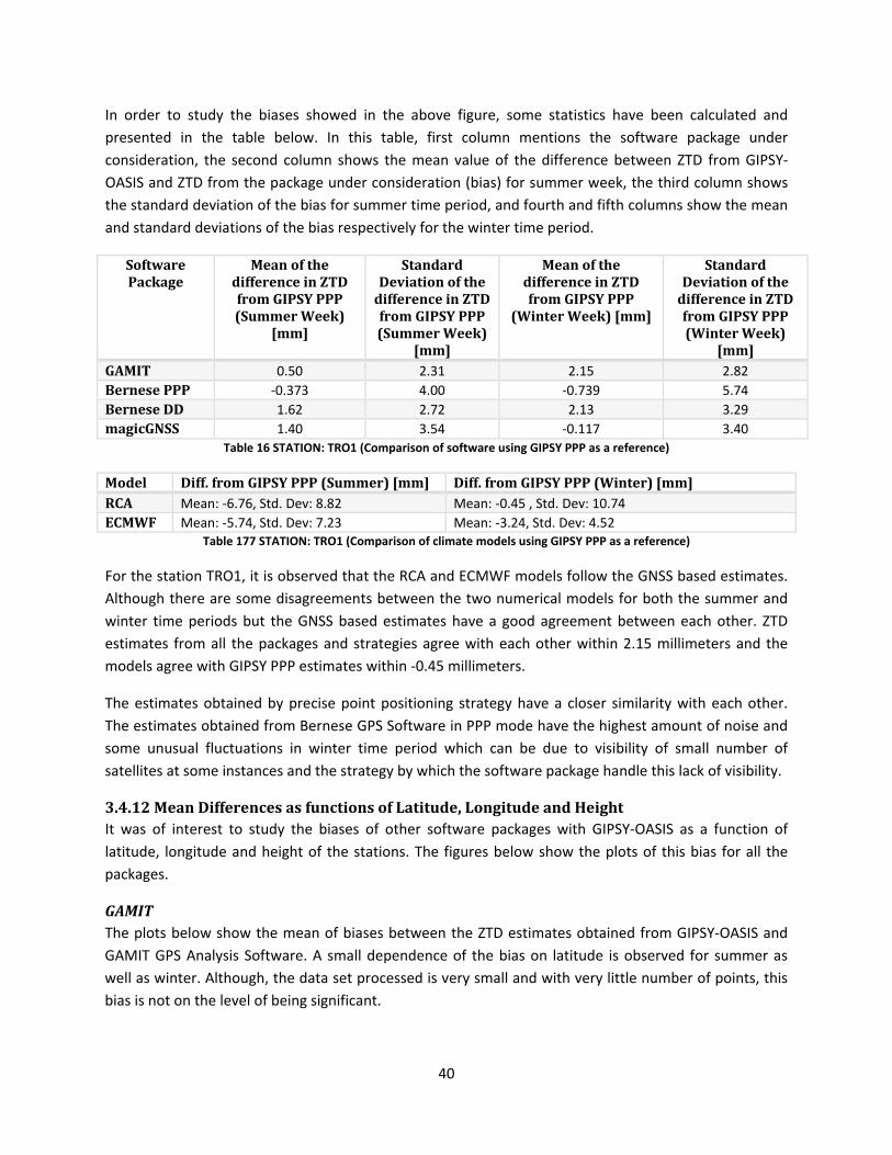
In order to study the biases showed in the above figure, some statistics have been calculated and presented in the table below. In this table, first column mentions the software package under consideration, the second column shows the mean value of the difference between ZTD from GIPSY‐OASIS and ZTD from the package under consideration (bias) for summer week, the third column shows the standard deviation of the bias for summer time period, and fourth and fifth columns show the mean and standard deviations of the bias respectively for the winter time period.
Software Package
Mean of the difference in ZTD from GIPSY PPP (Summer Week)
[mm]
Standard Deviation of the difference in ZTD from GIPSY PPP (Summer Week)
[mm]
Mean of the difference in ZTD from GIPSY PPP
(Winter Week) [mm]
Standard Deviation of the difference in ZTD from GIPSY PPP (Winter Week)
[mm] GAMIT 0.50 2.31 2.15 2.82Bernese PPP ‐0.373 4.00 ‐0.739 5.74Bernese DD 1.62 2.72 2.13 3.29magicGNSS 1.40 3.54 ‐0.117 3.40
Table 16 STATION: TRO1 (Comparison of software using GIPSY PPP as a reference)
Model Diff. from GIPSY PPP (Summer) [mm] Diff. from GIPSY PPP (Winter) [mm] RCA Mean: ‐6.76, Std. Dev: 8.82 Mean: ‐0.45 , Std. Dev: 10.74ECMWF Mean: ‐5.74, Std. Dev: 7.23 Mean: ‐3.24, Std. Dev: 4.52
Table 177 STATION: TRO1 (Comparison of climate models using GIPSY PPP as a reference)
For the station TRO1, it is observed that the RCA and ECMWF models follow the GNSS based estimates. Although there are some disagreements between the two numerical models for both the summer and winter time periods but the GNSS based estimates have a good agreement between each other. ZTD estimates from all the packages and strategies agree with each other within 2.15 millimeters and the models agree with GIPSY PPP estimates within ‐0.45 millimeters.
The estimates obtained by precise point positioning strategy have a closer similarity with each other. The estimates obtained from Bernese GPS Software in PPP mode have the highest amount of noise and some unusual fluctuations in winter time period which can be due to visibility of small number of satellites at some instances and the strategy by which the software package handle this lack of visibility.
3.4.12 Mean Differences as functions of Latitude, Longitude and Height It was of interest to study the biases of other software packages with GIPSY‐OASIS as a function of latitude, longitude and height of the stations. The figures below show the plots of this bias for all the packages.
GAMIT The plots below show the mean of biases between the ZTD estimates obtained from GIPSY‐OASIS and GAMIT GPS Analysis Software. A small dependence of the bias on latitude is observed for summer as well as winter. Although, the data set processed is very small and with very little number of points, this bias is not on the level of being significant.
40

60 65 70 75 80
0
2
4
Latitude [degree]
Mea
n B
ias
[mm
]
Difference between GAMIT and GIPSY (Summer)
-200 -100 0 100 200
0
2
4
Longitude [degree]
Mea
n B
ias
[mm
]
0 100 200 300 400 500
0
2
4
Height [m]
Mea
n B
ias
[mm
]
60 65 70 75 80
0
2
4
Latitude [degree]
Mea
n B
ias
[mm
]
Difference between GAMIT and GIPSY (Winter)
-200 -100 0 100 200
0
2
4
Longitude [degree]
Mea
n B
ias
[mm
]
0 100 200 300 400 500
0
2
4
Height [m]
Mea
n B
ias
[mm
]
Figure 37 Biases for GAMIT
41

magicGNSS The plots below show the mean of biases between the ZTD estimates obtained from GIPSY‐OASIS and magicGNSS. For this limited data set, no biases have been observed between magicGNSS and GIPSY‐OASIS.
60 65 70 75 80
0
2
4
Latitude [degree]
Mea
n B
ias
[mm
]
Difference between magicGNSS and GIPSY (Summer)
-200 -100 0 100 200
0
2
4
Longitude [degree]
Mea
n B
ias
[mm
]
0 100 200 300 400 500
0
2
4
Height [m]
Mea
n B
ias
[mm
]
60 65 70 75 80
0
2
4
Latitude [degree]
Mea
n B
ias
[mm
]
Difference between magicGNSS and GIPSY (Winter)
-200 -100 0 100 200
0
2
4
Longitude [degree]
Mea
n B
ias
[mm
]
0 100 200 300 400 500
0
2
4
Height [m]
Mea
n B
ias
[mm
]
Figure 38 Biases for magicGNSS
Bernese GPS Software (Double Difference Solution) The plots below show the mean of biases between the ZTD estimates obtained from GIPSY‐OASIS and Bernese GPS Software (Double Difference solution). No biases have been observed between GIPSY‐OASIS and Bernese GPS Software (Double Difference mode).
42

60 65 70 75 80
-2
0
2
4
Latitude [degree]
Mea
n B
ias
[mm
]
Difference between Bernese DD and GIPSY (Summer)
-200 -100 0 100 200
-2
0
2
4
Longitude [degree]
Mea
n B
ias
[mm
]
0 100 200 300 400 500
-2
0
2
4
Height [m]
Mea
n B
ias
[mm
]
60 65 70 75 80
-2
0
2
4
Latitude [degree]
Mea
n B
ias
[mm
]
Difference between Bernese DD and GIPSY (Winter)
-200 -100 0 100 200
-2
0
2
4
Longitude [degree]
Mea
n B
ias
[mm
]
0 100 200 300 400 500
-2
0
2
4
Height [m]
Mea
n B
ias
[mm
]
Figure 39 Biases for BSW (Double Difference Solution)
Bernese GPS Software (Precise Point Positioning Solution) The plots below show the mean of biases between the ZTD estimates obtained from GIPSY‐OASIS and Bernese GPS Software (Precise Point Positioning Solution). A small dependence of the bias on latitude is observed for summer time period. Although, the data set processed is very small and with very little number of points, this bias is not on the level of being significant.
43

60 65 70 75 80
-2
-1
0
1
Latitude [degree]
Mea
n B
ias
[mm
]
Difference between Bernese PPP and GIPSY (Summer)
-200 -100 0 100 200
-2
-1
0
1
Longitude [degree]
Mea
n B
ias
[mm
]
0 100 200 300 400 500
-2
-1
0
1
Height [m]
Mea
n B
ias
[mm
]
60 65 70 75 80
-2
-1
0
1
Latitude [degree]
Mea
n B
ias
[mm
]
Difference between Bernese PPP and GIPSY (Winter)
-200 -100 0 100 200
-2
-1
0
1
Longitude [degree]
Mea
n B
ias
[mm
]
0 100 200 300 400 500
-2
-1
0
1
Height [m]
Mea
n B
ias
[mm
]
Figure 40 Biases for BSW (Precise Point Positioning Solution)
3.5 Conclusions from Software Comparison In this part of the project, four software packages for GNSS data processing and two processing strategies have been compared by obtaining the estimate of zenith total delay by each of them. The estimates are obtained for one week each in summer and winter. It is observed that the zenith total delay estimates obtained by all the packages show a good agreement i.e. within 3 millimeters between each other. It is also observed that the solutions obtained using the precise point positioning strategy show a better agreement between each other.
There are some occasional offsets in outputs from different software packages which can be due to bad satellite geometry during that epoch and the method of a specific software package to handle that bad geometry.
The output from software packages has been validated using climate and weather models and it is observed that the Zenith Total Delay estimates obtained from GNSS data analysis has a good agreement with RCA and ECMWF climate and weather models.
There has been observed a small dependence of bias between GIPSY‐OASIS and GAMIT software packages on the latitude of station both for summer and winter time periods. For the summer time period, the bias between GIPSY‐OASIS and Bernese (for precise point positioning) software packages is seen to have a little dependence on station latitude.
44
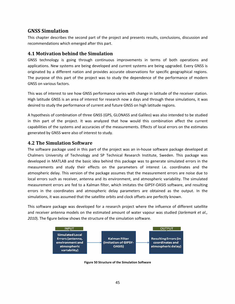
GNSS Simulation This chapter describes the second part of the project and presents results, conclusions, discussion and recommendations which emerged after this part.
4.1 Motivation behind the Simulation GNSS technology is going through continuous improvements in terms of both operations and applications. New systems are being developed and current systems are being upgraded. Every GNSS is originated by a different nation and provides accurate observations for specific geographical regions. The purpose of this part of the project was to study the dependence of the performance of modern GNSS on various factors.
This was of interest to see how GNSS performance varies with change in latitude of the receiver station. High latitude GNSS is an area of interest for research now a days and through these simulations, it was desired to study the performance of current and future GNSS on high latitude regions.
A hypothesis of combination of three GNSS (GPS, GLONASS and Galileo) was also intended to be studied in thin part of the project. It was analyzed that how would this combination affect the current capabilities of the systems and accuracies of the measurements. Effects of local errors on the estimates generated by GNSS were also of interest to study.
4.2 The Simulation Software The software package used in this part of the project was an in‐house software package developed at Chalmers University of Technology and SP Technical Research Institute, Sweden. This package was developed in MATLAB and the basic idea behind this package was to generate simulated errors in the measurements and study their effects on the parameters of interest i.e. coordinates and the atmospheric delay. This version of the package assumes that the measurement errors are noise due to local errors such as receiver, antenna and its environment, and atmospheric variability. The simulated measurement errors are fed to a Kalman filter, which imitates the GIPSY‐OASIS software, and resulting errors in the coordinates and atmospheric delay parameters are obtained as the output. In the simulations, it was assumed that the satellite orbits and clock offsets are perfectly known.
This software package was developed for a research project where the influence of different satellite and receiver antenna models on the estimated amount of water vapour was studied (Jarlemark et al., 2010). The figure below shows the structure of the simulation software.
Figure 50 Structure of the Simulation Software
45

4.3 Results from Simulation This section presents the results from various scenarios of the simulations.
The variations in the following results are due to the fact that it is not possible to simulate all the possible factors influencing the performance of the system. A small number of simulations has been performed and hence the uncertainty is not meaningful here.
The root mean square (RMS) value is a statistical measure of the magnitude of a varying quantity. The RMS value of a set of values can be calculated by taking the square root of the arithmetic mean of the squares of the original values. In this part of the project, all the simulations have been run 10 times and the obtained errors in the atmospheric delay are combined to get the RMS Error with better precision. Hence, in the graphs presented below, the RMS Error (y‐axis) implies the RMS value the effect (in millimeters) of local errors on atmospheric delay measurements.
4.3.1 GPS In this scenario, the constellation of modern GPS with 32 satellites was simulated to see the effect of local errors on the estimates of atmospheric delay. The ephemeris was generated by using orbit files from IGS. In the plot below, x‐axis contains latitudes ranging from ‐90o to 90o and y‐axis contains RMS value of error.
Figure 41 Effect of Local Errors on Atmospheric Delay Estimates from GPS
46

Overall RMS Error (GPS)
3.9 ± 0.13 mm
4.3.2 GLONASS In this scenario, the constellation of current GLONASS with 18 satellites was simulated to see the effect of local errors on the estimates of atmospheric delay. The ephemeris was generated by using orbit files from IGS. In the plot below, x‐axis contains latitudes ranging from ‐90o to 90o and y‐axis contains RMS value of error.
Figure 42 Effect of Loc imates from GLONASS al Errors on Atmospheric Delay Est
Overall RMS Error (GLONASS)
4.6 ± 0.26 mm
47

Here it is important to mention that the current GLONASS constellation which has been simulated in this project does not contain full number of satellites. In the above plot, one might interpret that GLONASS is less susceptible to local errors on latitudes above 0o but it is expected that when GLONASS starts operation with its full constellation, the effects of errors on latitudes between ‐90o to 0o would be reduced.
4.3.3 The Galileo System In this scenario, the constellation of future Galileo system with 30 satellites was simulated to see the effect of local errors on the estimates of atmospheric delay. The ephemeris was generated artificially using a MATLAB script. In the plot below, x‐axis contains latitudes ranging from ‐90o to 90o and y‐axis contains RMS value of error.
Figure 43 Effect of Loc Estimates from Galileo al Errors on Atmospheric Delay
Overall RMS Error (Galileo)
3.8 ± 0.13 mm
48

4.3.4 Combination of GPS, GLONASS and Galileo In this scenario, the hypothesis of combination of GPS, GLONASS and Galileo systems was tested by running a simulation with an ephemeris containing ephemeris from all GPS, GLONASS and Galileo systems. This simulation resulted in least amount of error. In the plot below, x‐axis contains latitudes ranging from ‐90o to 90o and y‐axis contains RMS value of error.
Figure 44 Effect of Local Error of GPS, GLONASS and Galileo s on Atmospheric Delay Estimates from Combination
Overall RMS Error (GPS + GLONASS + Galileo)
3.1 ± 0.07 mm
Here it can be seen that the overall RMS error has decreased significantly by using a combination of all the three systems. This combination can also result in increased reliability and robustness of the system.
49
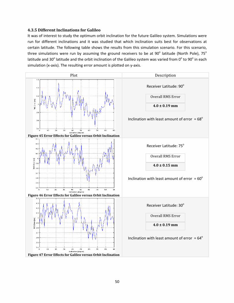
4.3.5 Different Inclinations for Galileo It was of interest to study the optimum orbit inclination for the future Galileo system. Simulations were run for different inclinations and it was studied that which inclination suits best for observations at certain latitude. The following table shows the results from this simulation scenario. For this scenario, three simulations were run by assuming the ground receivers to be at 90o latitude (North Pole), 75o latitude and 30o latitude and the orbit inclination of the Galileo system was varied from 0o to 90o in each simulation (x‐axis). The resulting error amount is plotted on y‐axis.
Plot Description
Figure 45 Error Effects for Galileo versus Orbit Inclination
Re 0o ceiver Latitude: 9
Overall RMS Error
4.0 ± 0.19 mm
Inclination with least amount of error = 68o
Figure 46 Error Effects for Galileo versus Orbit Inclination
Re 5o ceiver Latitude: 7
Overall RMS Error
4.0 ± 0.15 mm
Inclination with least amount of error = 60o
Figure 47 Error Effects for Galileo versus Orbit Inclination
Re 0o ceiver Latitude: 3
Overall RMS Error
4.0 ± 0.19 mm
Inclination with least amount of error = 64o
50
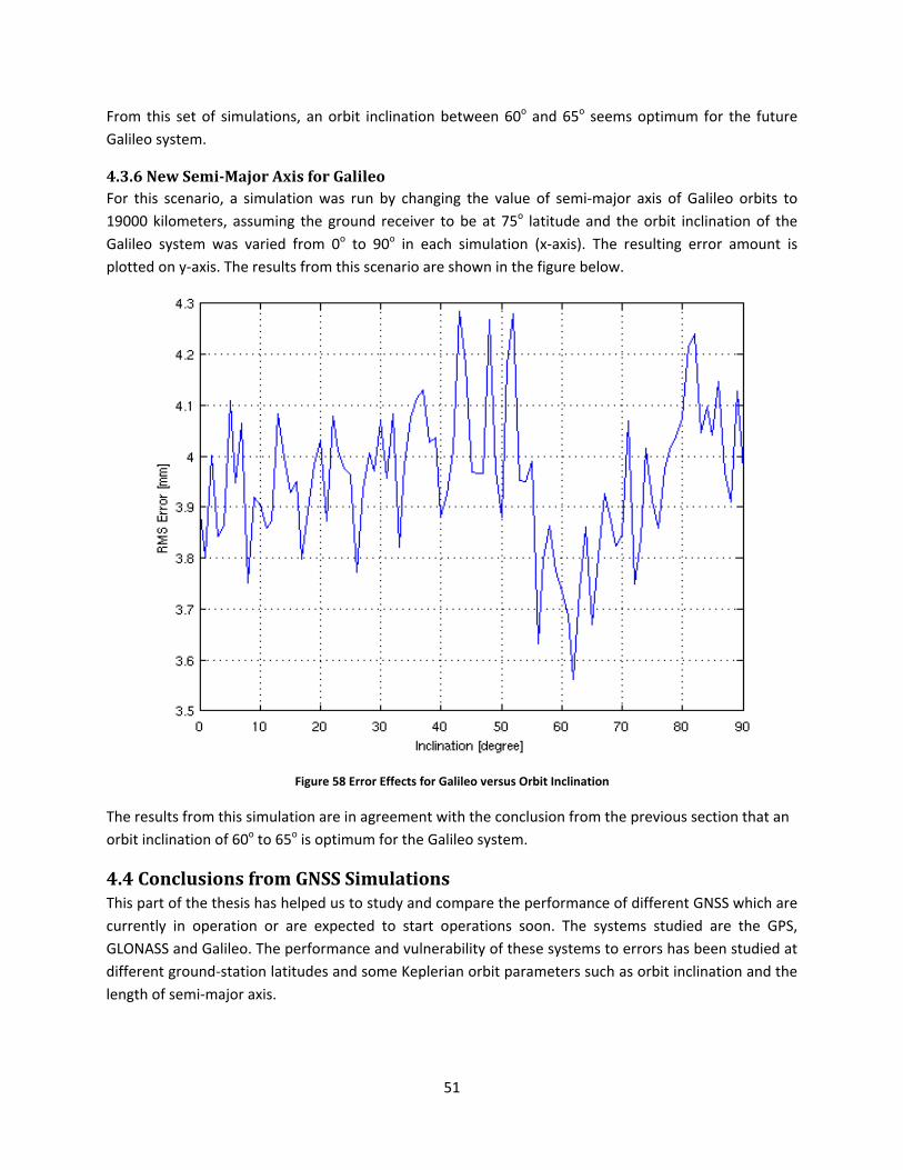
From this set of simulations, an orbit inclination between 60o and 65o seems optimum for the future Galileo system.
4.3.6 New SemiMajor Axis for Galileo For this scenario, a simulation was run by changing the value of semi‐major axis of Galileo orbits to 19000 kilometers, assuming the ground receiver to be at 75o latitude and the orbit inclination of the Galileo system was varied from 0o to 90o in each simulation (x‐axis). The resulting error amount is plotted on y‐axis. The results from this scenario are shown in the figure below.
Figure 58 Error Effects for Galileo versus Orbit Inclination
The results from this simulation are in agreement with the conclusion from the previous section that an orbit inclination of 60o to 65o is optimum for the Galileo system.
4.4 Conclusions from GNSS Simulations This part of the thesis has helped us to study and compare the performance of different GNSS which are currently in operation or are expected to start operations soon. The systems studied are the GPS, GLONASS and Galileo. The performance and vulnerability of these systems to errors has been studied at different ground‐station latitudes and some Keplerian orbit parameters such as orbit inclination and the length of semi‐major axis.
51

From the first type of simulations, the atmospheric delay parameters obtained from GPS, GLONASS and Galileo are compared with each other in terms of vulnerability to local errors such as antenna phase center variations, environment of the receiver and atmospheric variability. The results show that GLONASS has the highest susceptibility to local errors and the overall RMS value of resulting error in atmospheric delay from GLONASS is 4.6 millimeters. For GPS and Galileo, these values are 3.9 and 3.8 millimeters respectively which shows that the current GPS and the future Galileo have nearly the same susceptibility to local errors. Also, it is worth mentioning that the current GLONASS is far more vulnerable to local errors than the GPS and Galileo.
In the second type of simulation, a new system has been proposed which has the constellations of GPS, GLONASS and Galileo combined in it. Then it is studied that how would this proposed system perform in terms of susceptibility to local errors. A significant reduction in the effects of local errors has been observed in the results of this simulation and the new system has an overall RMS value of 3.1 millimeters error effects which is 0.7 millimeters less than that of Galileo, 0.8 millimeters less than that of GPS and 1.5 millimeters less than that of GLONASS. The proposed new system has an increased reliability and robustness.
The third type of simulations were related to the study of an optimum orbit inclination for the future Galileo system. The effect of local errors on atmospheric delay estimates on different ground‐station latitudes were studied as a function of orbit inclination. As a special case, the semi‐major axis of Galileo orbits was changed to 19,000 kilometers in one of the simulations and the error effects were studies for varying inclinations. From all the simulations of this kind, it was noticed that for orbit inclinations between 60o and 65o, the estimates have least amount of error.
52

Recommendations This chapter contains the recommendations for possible future work which emerged after this project. Recommendation from each of the two parts of the project are presented in two different sections.
5.1 Recommendations from Software Comparison This project has set a strategy for comparison of GNSS software packages and climate models. This strategy can be used to perform such a comparison using extensive data sets containing data for several years (e.g. 5 years or more). This will result in improved certainty in the results.
Software packages can be compared using different processing criteria than those used in this project. There can be new choices of tropospheric mapping functions used for the reason that new mapping functions are being developed nowadays. Use of lower elevation cut‐off angles in the criteria in combination with modern mapping functions can also be of interest to study.
In this project, the comparison was based on observations from GPS only. This comparison can be extended to include GLONASS observations as three of the software packages i.e. GIPSY‐OASIS, Bernese GPS Software, and magicGNSS are capable of handling GLONASS.
5.2 Recommendations from GNSS Simulations In this project, the simulations of future GNSS have been run by varying the orbit inclinations and the value of the semi‐major axis. These simulations can be performed by varying other Keplerian orbit parameters to optimize the choice of parameters for the future Galileo system.
The simulations of the Chinese Compass Navigation Satellite System (CNSS) can be carried out to study the effects of local errors on its observations.
53

Bibliography Achberger, C., Linderson , M.‐L., and Chen,D. (2003), Performance of the Rossby Centre regional atmospheric model in Southern Sweden: comparison of simulated and observed precipitation, Theor. Appl. Climatol. 76, 219–234, DOI 10.1007/s00704‐003‐0015‐6 B. Hofmann‐Wellenhof,H. Lichtenegger,J.Collins, Global Positioning System: Theory and Practice (ISBN:3211825916 / 3‐211‐82591‐6)
Bevis, M., S. Businger, Chiswell S., T. A. Herring, R. A. Anthes, C. Rocken, R. H. Ware, GPS Meteorology: Mapping Zenith Wet Delays onto Precipitable Water, Journal of Applied Meteorology, vol. 33, pp. 379~386. Bevis, M., S. Businger, T. A. Herring, C. Rocken, R. A. Anthes, and R. H. Ware, GPS Meteorology: Remote Sensing of atmospheric water vapour using the Global Positioning System Journal of Geophysics, Res., 97, 15 787‐15 801. Dach, R., U. Hugentobler, P. Fridez, and M. Meindl (Eds.) (2007), Bernese GPS Software Version 5.0, 612 pp., Atronomical Institute, University of Bern Bern.
Dow, J.M., Neilan, R. E., and Rizos, C., The International GNSS Service in a changing landscape of Global Navigation Satellite Systems, Journal of Geodesy (2009) 83:191–198, DOI: 10.1007/s00190‐008‐0300‐3.
Gorres, B., J. Campbell, M. Becker, and M. Siemes, Absolute calibration of GPS antennas: laboratory results and comparison with field and robot techniques, GPS Sol 10(2), 136~145, DOI: 10.1007/s10291‐005‐0015‐3, 2005. Herring, T. A. (2005), GLOBK Global Kalman filter VLBI and GPS analysis program version 10.1, Dept. of Earth, Atmospheric, and Planetary Sciences, Mass. Inst. of Technol., Cambridge, USA.
Herring, T. A., Modeling Atmospheric Delays in the Analysis of Space Geodetic Data, in Symposium on Refraction of Transatmospheric Signals in Geodesy, J. C. DeMunk and T. A. Spoelstra, eds., Netherlands Geodetic Commission Series No. 36, 157‐164, 1992. J. Nash, E. J. Orliac, A. H. Dodson, R. M. Bingley, J. Jones, and F. N. Teferle. On the use of near real‐time gps inferred humidity fields for monitoring thunderstorm activity. Eos Transactions, 87(52), 2006. A11E‐08. Jarlemark, P.O.J., R. Emardson, J.M. Johansson, and G. Elgered, Ground‐Based GPS for Validation of Climate Models: the impact of Satellite Antenna Phase Center Variations IEEE Geosci. Rem. Sens., submitted, 2010. Johansson J M, Davis J L, Scherneck H‐G, Milne G A, Vermeer M, Mitrovica J X, Bennett R A, Jonsson B, Elgered G, Elósegui P, Koivula H, Poutanen M, Rönnäng B O, Shapiro I I (2002). Continuous GPS measurements of postglacial adjustment in Fennoscandia 1. Geodetic result. J. Geophys. Res., 107(B8), 2157, doi:10.1029/2001 JB000400.
54
55
Jung, T., Balsamo, G., et al., 2010, The ECMWF model climate: recent progress through improved physical parameterizations, DOI: 10.1002/qj.634 Álvaro Mozo García, Ricardo Píriz, Miguel M. Romay Merino, 2008, magicGNSS: Quality Data, Algorithms and Products for the GNSS User Community, IS‐GPS/GNSS 2008 Mäkinen J., H. Koivula, M. Poutanen, V. Saaranen (2003): Vertical velocities in Finland from permanent GPS networks and from repeated precise leveling. Journal of Geodynamics, 38, 443‐456. Niell, A.E. Global mapping functions for the atmosphere delay at radio wavelengths, Haystack Observatory, Massachusetts Institute of Technology, Westford, J.G.R. 101, b2, 3227‐3246, 1996 corrected) Orliac, Etienne J. (2009) Development of azimuth dependent tropospheric mapping functions, based on a high resolution mesoscale numerical weather model, for GNSS data processing. PhD thesis, University of Nottingham. Ortiz de Galisteo, J. and Toledano, C. and Cachorro, V. and Torres, B., Improvement in PWV estimation from GPS due to the absolute calibration of antenna phase center variations, GPS Solutions, vol. 14, no. 4, pp. 389~395, 2010. T. Ning, G. Elgered, and J.M. Johansson, The Impact of Microwave Absorber and Radome Geometries on Geodetic Measurements With Ground‐Based GNSS Antennas, Submitted to Advances in Space Research, 2010.
Zumberge, J. F., Heftin, M. B., Jefferson, D.C., Watkins, M. M. (1997), Precise point positioning for the efficient and robust analysis of GPS data from large networks, JOURNAL OF GEOPHYSICAL RESEARCH (102), NO. B3, 5005‐5017


![KTU-GEOD IVS Analysis Center Biennial Report (2017-2018)2018/... · 2019. 12. 26. · KTU-GEOD Biennial Report (2017–2018) 219 ing modified Bernese software [4] by the GNSS anal-ysis](https://static.fdocuments.us/doc/165x107/60be53de54ac482d5751e6a4/ktu-geod-ivs-analysis-center-biennial-report-2017-2018-2018-2019-12-26.jpg)