Evaluation of FWD software and deflection basin for ...
198
University of New Mexico UNM Digital Repository Civil Engineering ETDs Engineering ETDs 9-3-2010 Evaluation of FWD soſtware and deflection basin for airport pavements Mesbah Uddin Ahmed Follow this and additional works at: hps://digitalrepository.unm.edu/ce_etds is esis is brought to you for free and open access by the Engineering ETDs at UNM Digital Repository. It has been accepted for inclusion in Civil Engineering ETDs by an authorized administrator of UNM Digital Repository. For more information, please contact [email protected]. Recommended Citation Ahmed, Mesbah Uddin. "Evaluation of FWD soſtware and deflection basin for airport pavements." (2010). hps://digitalrepository.unm.edu/ce_etds/30
Transcript of Evaluation of FWD software and deflection basin for ...

University of New MexicoUNM Digital Repository
Civil Engineering ETDs Engineering ETDs
9-3-2010
Evaluation of FWD software and deflection basinfor airport pavementsMesbah Uddin Ahmed
Follow this and additional works at: https://digitalrepository.unm.edu/ce_etds
This Thesis is brought to you for free and open access by the Engineering ETDs at UNM Digital Repository. It has been accepted for inclusion in CivilEngineering ETDs by an authorized administrator of UNM Digital Repository. For more information, please contact [email protected].
Recommended CitationAhmed, Mesbah Uddin. "Evaluation of FWD software and deflection basin for airport pavements." (2010).https://digitalrepository.unm.edu/ce_etds/30


ii
EVALUATION OF FWD SOFTWARE AND DEFLECTION BASIN FOR AIRPORT PAVEMENTS BY MESBAH UDDIN AHMED B. Sc. in Civil Engineering Bangladesh University of Engineering and Technology, Dhaka, Bangladesh THESIS Submitted in Partial Fulfillment of the Requirements for the Degree of MASTER OF SCIENCE Civil Engineering The University of New Mexico Albuquerque, New Mexico July, 2010

iii
© 2010, Mesbah Uddin Ahmed

iv
DEDICATION
To my parents

v
AKNOWLEDGEMENTS
I would like to thank Dr. Rafiqul A. Tarefder, my supervisor and thesis committee chair,
for his support, time and encouragement for this study. His guidance and professional
style will remain with me as I continue my career.
I would like to thank my thesis committee members: Dr. Tang-Tat Ng and Dr. John C.
Stormont for their valuable recommendations pertaining to this study.
I would like to express my gratitude to the Aviation Department, New Mexico
Department of Transportation (NMDOT) for the funding to pursue this research. I would
like to thank Jane Lucero, Administrator, Aviation Department and Robert McCoy of
Material Bureau, NMDOT for their assistance in field data collection.
Co-operation and encouragement from the team members of my research group are
highly appreciated. I thank Raju Bisht and Ryan W. Webb for their sincere effort in
laboratory testing for this study. Motivation from my friend, a graduate student Late
Mohammad Minhaz Mahdi is greatly acknowledged.

vi
EVALUATION OF FWD SOFTWARE AND DEFLECTION BASIN
FOR AIRPORT PAVEMENTS
BY
MESBAH UDDIN AHMED
ABSTRACT OF THESIS
Submitted in Partial Fulfillment of the
Requirements for the Degree of
MASTER OF SCIENCE
Civil Engineering
The University of New Mexico
Albuquerque, New Mexico
July 2010

vii
EVALUATION OF FWD SOFTWARE AND DEFLECTION BASIN FOR AIRPORT PAVEMENTS
by
Mesbah Uddin Ahmed
M. Sc. in Civil Engineering, University of New Mexico
Albuquerque, NM, USA 2010
B. Sc. in Civil Engineering, Bangladesh University of Engineering and Technology
Dhaka, Bangladesh 2007
ABSTRACT
Falling Weight Deflectometer (FWD) test data are processed by backcalculation software
to obtain modulus of layer materials of airport pavements. Currently, several
backcalculation software are available. However it is not known which software produces
accurate and consistence modulus values. In this study three backcalculation software;
namely, BAKFAA, EVERCALC, and MODULUS are evaluated for consistency and
accuracy. To examine accuracy, software predicted modulus values are compared to the
laboratory tested modulus values of soils, aggregate, and asphalts. Consistency is
examined by statistical analysis using three sets of FWD deflection data produced by
three loads with magnitudes of 9, 12, and 16 kip at an identical location of an airport
pavement. It is shown that EVERCALC software produces more consistent and accurate
modulus values than the BAKFAA and MODULUS software.
A concern with the available backcalculation software is that their analysis algorithms are
based on layered elastic theory with linear materials models. In addition, they consider
static loading, which is not the true representation of the dynamic loads applied in a FWD

viii
test in the field. To this end, this study performs a dynamic analysis of the FWD
deflection basin using a finite element method (FEM) with the consideration of non-
linear materials models. Results show that FEM predicted deflections have similar trends
of the field measured deflections. However, a number of trial combinations of inputs and
FEM models may be required to produce an identical match between the predicted and
measured deflections. It is recommended that this approach be the subject of future
studies.

ix
TABLE OF CONTENTS
ABSTRACT ................................................................................................................................. vii
CHAPTER 1 .................................................................................................................................. 1
INTRODUCTION ........................................................................................................................ 1
1.1 Introduction ..........................................................................................................1
1.2 Problem Statement ...............................................................................................1
1.3 Hypothesis ............................................................................................................3
1.4 Objectives .............................................................................................................4
CHAPTER 2 .................................................................................................................................. 6
LITERATURE REVIEW ............................................................................................................ 6
2.1 Introduction ...............................................................................................................6
2.2 FWD Test ..................................................................................................................6
2.2.1 KUAB FWD ...........................................................................................................7
2.2.2 Dynatest FWD ........................................................................................................7
2.2.3 Carl Bro FWD ........................................................................................................7
2.2.4 JILS FWD ..............................................................................................................8
2.3 Current Applications of FWD test ............................................................................8
2.4 Backcalculation of Layer Moduli ..............................................................................9
2.4.1 Boussinesq’s Solution Method .............................................................................10
2.4.2 Multi-Layered Elastic Theory ..............................................................................12
2.4.3 Finite Element Method .........................................................................................15
2.5 Overview of Backcalculation Software ...................................................................16
2.5.1 BISDEF ................................................................................................................16
2.5.2 BOUSDEF ............................................................................................................17
2.5.3 CHEVDEF ...........................................................................................................17
2.5.4 ISSEM4 ................................................................................................................18
2.5.5 ELMOD ................................................................................................................18
2.5.6 ELSEDEF .............................................................................................................19
x
2.5.7 LOADRATE ........................................................................................................19
2.5.8 MODCOMP2 .......................................................................................................20
2.5.9 OAF ......................................................................................................................20
2.5.10 FWD AREA .......................................................................................................20
2.5.11 SEARCH ............................................................................................................21
2.5.12 WESDEF ............................................................................................................21
2.5.13 VESYS ...............................................................................................................22
2.6 Research Background ..............................................................................................22
CHAPTER 3 ................................................................................................................................ 31
BACKCALCULATION METHODOLOGY ........................................................................... 31
3.1 Introduction .............................................................................................................31
3.2 Principle of Backcalculation ...................................................................................31
3.3 FAA Guidelines for Backcalculation ......................................................................32
3.3.1 Data Collection .....................................................................................................32
3.3.2 Factors Responsible for Analysis Anomalies .......................................................33
3.3.3 Analysis ................................................................................................................36
3.3.4 Review of Backcalculated Modulus .....................................................................37
3.4 Backcalculation Software ........................................................................................37
3.4.1 BAKFAA .............................................................................................................38
3.4.2 MODULUS 6.0 ....................................................................................................38
3.4.3 EVERCALC 5.0 ...................................................................................................39
3.4.4 AASHTO 1993 .....................................................................................................40
3.5 Factors Affecting Backcalculated Modulus ............................................................42
3.5.1 Loading .................................................................................................................42
3.5.2 Climate .................................................................................................................42
3.5.3 Pavement Condition .............................................................................................44
3.6 Backcalculation in Airport Pavement Evaluation ...................................................44
3.7 Summary .................................................................................................................45
CHAPTER 4 ................................................................................................................................ 53
ACCURACY AND CONSISTENCY ........................................................................................ 53

xi
4.1 Introduction .............................................................................................................53
4.2 Objectives ................................................................................................................53
4.3 Study Approach .......................................................................................................54
4.4 Data Collection and Testing Plan ............................................................................54
4.4.1 FWD Testing ........................................................................................................55
4.4.2 Asphalt Coring and Soil Sampling in the Field ....................................................56
4.5 Laboratory Testing ..................................................................................................57
4.5.1 Resilient Modulus of Asphalt Concrete ...............................................................57
4.5.2 Indirect Tensile Strength of Asphalt Concrete .....................................................59
4.6 Consistency of the Software ....................................................................................60
4.6.1 Frequency Plot of Mr ............................................................................................60
4.6.2 Frequency Plot of CV of Mr .................................................................................61
4.7 Accuracy of the Software ........................................................................................64
4.7.1 Backcalculated vs. Measured Modulus of Asphalt Concrete ...............................64
4.7.2 Backcalculated vs. Measured Modulus of Subgrade ...........................................65
4.8 Backcalculated vs. Measured Tensile Strength of Asphalt Concrete ......................67
4.9 Conclusion ...............................................................................................................69
CHAPTER 5 ................................................................................................................................ 86
FINITE ELEMENT MODELING OF FWD DEFLECTION ................................................ 86
5.1 Introduction .............................................................................................................86
5.2 Objectives ................................................................................................................86
5.3 FEM Model Description ..........................................................................................87
5.3.1 Model Geometry ..................................................................................................88
5.3.2 Layer Property ......................................................................................................92
5.3.3 Meshing of Model ................................................................................................95
5.3.4 Boundary Condition .............................................................................................97
5.3.5 Loading Criteria ...................................................................................................99
5.4 Finite Element Analysis ........................................................................................100
5.4.1 Static Analysis ....................................................................................................100
5.4.2 Dynamic Analysis ..............................................................................................101
xii
5.5 Discussion .............................................................................................................102
5.5.1 Static Deflection Basin .......................................................................................102
5.5.2 Dynamic Deflection Basin and Time History ....................................................105
5.5.5 Deflection at Layer .............................................................................................112
5.5.4 Contour of Vertical Deflection ...........................................................................113
5.5.5 Contour of Stress ................................................................................................115
5.6 Comparing Static vs. Dynamic Analysis ...............................................................116
5.7 Conclusions ...........................................................................................................117
CHAPTER 6 .............................................................................................................................. 154
CONCLUSIONS ....................................................................................................................... 154
REFERENCES .......................................................................................................................... 158
APPENDICES ........................................................................................................................... 166

xiii
LIST OF TABLES
Table 3.1: FWD test plan ............................................................................................................... 47
Table 4.1: Borehole information in Runway 2-20 (Raton municipal airport) ............................... 71
Table 4.2: Thicknesses of the Layers and Subgrade Soil Classification ........................................ 72
Table 4.3: Resilient Modulus and Indirect Tensile Strength of Asphalt Core ............................... 73
Table 4.4: CV of a test location (MP 6000 ft.) at Runway 8-26 at Silvercity Airport ................. 74
Table 5.1: Modulus of elasticity of flexible pavement layer ....................................................... 118
Table 5.2: Parameters of the finite element model ...................................................................... 119
Table 5.3: Vertical deflection at the layer interface ..................................................................... 120

xiv
LIST OF FIGURES
Figure 2.1: FWD test and the pavement surface response ............................................................. 28
Figure 2.2: Generalized pavement response under uniformly distributed load (Boussisnesq, 1885) ....................................................................................................................................................... 29
Figure 2.3: Multi-layered pavement structure ................................................................................ 30
Figure 3.1: Flow chart of the backcalculation of layer moduli ...................................................... 48
Figure 3.2: Different types of anomalies in deflection type.......................................................... 49
Figure 3.3: Rigid layer depth determination .................................................................................. 50
Figure 3.4: Generalized plan of FWD test ..................................................................................... 51
Figure 3.5: Layer thickness consideration for the analysis ............................................................ 52
Figure 4.1: Data collection Raton Municipal Airport .................................................................... 75
Figure 4.2: Laboratory resilient modulus and Indirect tensile strength test ................................... 76
Figure 4.3: Frequency distribution of the surface modulus ........................................................... 77
Figure 4.4: Frequency distribution of base modulus ...................................................................... 78
Figure 4.5: Frequency distribution subgrade modulus ................................................................... 79
Figure 4.6: Frequency distribution of coefficient of variation of the analysis ............................... 80
Figure 4.7: Backcalculated surface modulus vs. Laboratory resilient modulus (9 kip load) ......... 81
Figure 4.8: Backcalculated surface modulus vs. Laboratory resilient modulus ............................. 82
Figure 4.9: Backcalculated modulus vs. Subgrade modulus for accuracy ..................................... 83
Figure 4.10: Tensile stress developed at the bottom of the surface course .................................... 84
Figure 4.11: Backcalculated vs. Laboratory tensile strength ......................................................... 85
Figure 5.1: The zone of influence during FWD test .................................................................... 121
Figure 5.2: Qualitative diagram of the Axi-symmetric model of flexible pavement ................... 122
Figure 5.3: Qualitative diagram of the Quarter cube model of flexible pavement ...................... 123
Figure 5.4: Stress-strain distribution of the granular soil in base course (Garg and Thompson, 1997) ............................................................................................................................................ 124

xv
Figure 5.5: Stress-strain distribution of subgrade soil from triaxial test (Slope stability 2003) .. 125
Figure 5.6: Mesh refinement of the axi-symmetric model ........................................................... 126
Figure 5.7: Mesh refinement of the quarter cube model .............................................................. 127
Figure 5.8: Amplitude pattern of the impulse in the FWD test .................................................... 128
Figure 5.9: Time-deflection histories of the sensors .................................................................... 129
Figure 5.10: Deflection basins analyzed for different layer moduli combinations (axi-symmetric static analysis) .............................................................................................................................. 130
Figure 5.10: Deflection basins analyzed for different layer moduli combinations (axi-symmetric static analysis) .............................................................................................................................. 131
Figure 5.11: Deflection basins analyzed for different layer moduli combinations (quarter cube static analysis) .............................................................................................................................. 132
Figure 5.11: Deflection basins analyzed for different layer moduli combinations (quarter cube static analysis) .............................................................................................................................. 133
Figure 5.12: Deflection basins analyzed for different layer moduli combinations (axi-symmetric dynamic analysis)......................................................................................................................... 134
Figure 5.12: Deflection basins analyzed for different layer moduli combinations (axi-symmetric dynamic analysis)......................................................................................................................... 135
Figure 5.13: Time-deflection histories at the sensors for layer moduli combinations (axi-symmetric dynamic analysis) ....................................................................................................... 136
Figure 5.13: Time-deflection histories at the sensors for layer moduli combinations (axi-symmetric dynamic analysis) ....................................................................................................... 137
Figure 5.14: Deflection basins analyzed for different layer moduli combinations (quarter cube dynamic analysis)......................................................................................................................... 138
Figure 5.14: Deflection basins analyzed for different layer moduli combinations (quarter cube dynamic analysis)......................................................................................................................... 139
Figure 5.15: Time-deflection histories at the sensors for layer moduli combinations (quarter cube dynamic analysis)......................................................................................................................... 140
Figure 5.15: Time-deflection histories at the sensors for layer moduli combinations (quarter cube dynamic analysis)......................................................................................................................... 141
Figure 5.16: Contour of vertical deflection (200, 40, and 8 ksi) .................................................. 142
Figure 5.17: Contour of vertical deflection (300, 40, and 24 ksi) ................................................ 143

xvi
Figure 5.18: Contour of vertical deflection (200, 40, and 8 ksi) .................................................. 144
Figure 5.19: Contour of vertical deflection (300, 40, and 24 ksi) ................................................ 145
Figure 5.20: Contour of von Mises stress (200, 40, and 8 ksi) .................................................... 146
Figure 5.21: Contour of von Mises stress (300, 40, and 24 ksi) .................................................. 147
Figure 5.22: Contour of von Mises stress (200, 40, and 8 ksi) .................................................... 148
Figure 5.23: Contour of von Mises stress (300, 40, and 24 ksi) .................................................. 149
Figure 5.24: Comparison of FWD deflection basins (axi-symmetric) ......................................... 150
Figure 5.24: Comparison of FWD deflection basins (axi-symmetric) ......................................... 151
Figure 5.25: Comparison of FWD deflection basins (quarter cube) ............................................ 152
Figure 5.25: Comparison of FWD deflection basins (quarter cube) ............................................ 153
1
CHAPTER 1
INTRODUCTION
1.1 Introduction
Falling Weight Deflectometer (FWD) is a widely used nondestructive test to measure the
pavement surface deflection for the evaluation of pavement structural capacity. In this
test, an impulse is generated on the surface by dropping a weight from a pre-defined
height. The load is then transmitted to the pavement through a circular steel plate. In
response to the applied load, the pavement surface moves vertically downward and thus,
forms a deflection basin. Geophones located at different offsets from loading point
measure these vertical deflections. These deflection data are then processed to evaluate
the pavement strength in terms of layer modulus. This layer modulus determined from
known FWD data is termed as backcalculated modulus. A number of commercial and
non-commercial software are available for the analysis of FWD data to obtain
backcalculated layer modulus. The backcalculated modulus is not only used in design but
also to determine the remaining life of the pavement, thus, the role of this layer modulus
is significant in pavement engineering. This study focuses on the evaluation of the
backcalculated layer modulus.
1.2 Problem Statement
The available backcalculation software have some drawbacks in determining
backcalculated modulus. Limited study was done before on these aspects. To date, a
rigorous study has not been carried out to evaluate the backcalculated modulus.

2
Accuracy is one of the limitations of the backcalculated modulus from these software. It
is necessary for the backcalculated moduli to be the same or very close to the laboratory
test data. If the backcalculated modulus is higher than the laboratory determined
modulus, it will lead towards the under-design of the pavement. Conversely, the lower
backcalculated modulus may result in over-design of the pavement thickness, and the
resulting design will not be economical. To forecast the remaining life of a pavement, the
accuracy of the backcalculated modulus plays a significant role. A backcalculated
modulus that is greater than the actual modulus will result in the predicted remaining life
being greater than the actual life. If necessary maintenance is not applied, the overlay
design will not be adequate to provide the pavement with necessary structural capacity.
On the other hand, a backcalculated modulus that is lower than the actual modulus will
result in a shorter predicted remaining life. Consequently, the design produces a
maintenance cost greater than actually required. Therefore, it is necessary to examine the
accuracy of the backcalculation software.
Another problem associated with the backcalculation software is the lack of consistency
of the results in that backcalculated moduli determined using different loads are not the
same. According to the requirements of ASTM D 4694, different magnitudes of loads are
applied in FWD test. The backcalculated moduli at a test section should be the same or at
least very close to each other for different load levels. If the differences between the
backcalculated moduli from the software are significant, the software can be considered
to have a lack of consistency. The lack of consistency raises the question about the
applicability of the backcalculated layer modulus. So, it is important to understand on the
consistency of the backcalculation software.
3
Most commercial software is based on the layered elastic analysis. Some software
packages have the option to integrate 2D Finite Element Modeling (FEM) of pavement
into the analysis. There are also a few non-commercial software uses the 3D finite
element modeling in the analysis of FWD data. Most of the 3D finite element modeling
considers the FWD loading to be static. However, the FWD test load is not the static. The
load applied in the FWD test is dynamic, that is, the load varies with time. For the 3D
modeling of the flexible pavement with dynamic load, some of the studies consider the
haversine load applied on the pavement surface (Lukanen 1993, Hoffman 1983, Nazarian
1995, and Sebaaly et al 1986). However, this is not a true representation of the FWD
load. Therefore, the time-deflection history determined from those modeling may not be
appropriate for the FWD data analysis. This suggests the application of 3D finite
modeling requires more understanding.
1.3 Hypothesis
A number of commercial software has the lack in accuracy and/or consistency of the
backcalculated modulus. The applicability of these backcalculated layer moduli needs to
be evaluated. For comparison to the backcalculated modulus from these software, moduli
were determined from laboratory tests conducted on asphalt concrete samples collected
from airport pavements. To investigate the consistency of the backcalculated modulus,
the statistical analysis is done in this study.
The 3D finite element modelings of the flexible pavement in the previous studies have
considered the dynamic load with the haversine load pattern. This loading pattern does
not represent loading measured in the field (Nazarian 1995). Therefore, the results from

4
these analyses were not good enough to represent the field response. For this reason, this
study focuses on the 3D finite element modeling of FWD deflection basin with an
impulse dynamic load. The response of the pavement is determined in terms of time-
deflection history, i.e., the deflection varies with time at each sensor (geophone). The
time-deflection history from this model can be used for the backcalculation of the layer
modulus.
1.4 Objectives
The first hypothesis has recommended some objectives and these are:
- Analyze FWD data to backcalculate modulus using different backcalculation
software.
- Perform laboratory tests for determining resilient modulus and indirect tensile
strength of the asphalt concrete. Compare the analysis results with the laboratory
test data to check the accuracy of the software.
- Compare the backcalculated modulus for a single point at three different loads to
evaluate the consistency of their analysis.
A number of researchers used the MODULUS and EVERCALC for their study (Ameri et
al 2009, Yin and Mrawira 2009, Rahim and George 2003, and Mahoney et al 1989) and
these are widely used for the strength evaluation in highway pavement. Federal Aviation
Administration (FAA) developed a backcalculation software BAKFAA to process the
FWD data from airport pavement (Larkin and Hayhoe 2009). For this reason, three
software MODULUS 6.0, EVERCALC 5.0, and BAKFAA are used in this study.

5
The objectives under the second hypothesis are:
- To generate the time-deflection histories at the sensor points of the flexible
pavement under the impulse during the FWD test using 3D Finite Element
Method.
- To study the variations of the time-deflection history with the variations in layer
properties, thickness, and the depth to rigid layer.
- To perform static analysis and observe the deviation of the analysis results from
dynamic analysis.

6
CHAPTER 2
LITERATURE REVIEW
2.1 Introduction
FWD test for the pavement strength evaluation plays an important role in the pavement
engineering since its inception in early 1980’s. Since then, several methods have been
developed for the investigation of the structural capacity of the pavement layers using
FWD data. This chapter focuses on the current practices of the pavement strength
evaluation by FWD test, the data processing methods, and FWD’s applicability in the
pavement design and maintenance. A brief discussion of research regarding FWD data
analysis methodologies and the pavement deflection modeling are covered in this chapter.
2.2 FWD Test
In this test, an impulse load is generated on the pavement surface by dropping a weight
on a circular plate of 12 to 18 in. diameter from a height of 1.5 to 2 ft using a spring-mass
system. The duration of the load is about 20 to 35 milliseconds. The steel plate comes to
a smooth contact with the surface of the pavement by the use of a rubber pad. Pavement
deflections are measured by seven geophones resting longitudinally on the surface. A
photograph taken during initial setup of the FWD testing assembly is shown in Figure
2.1(a). Due to the application of the dynamic load, the pavement surface deflects
vertically downward forming a deflection basin. Figure 2.1(b) is a schematic of a
deflection basin. The FWD device can accommodate seven to nine sensors for the
measurement of vertical deflections. However, in this study seven geophones are used at
different radial offset from the load. The distances of the geophones from the center of

7
the loading plate are 0, 8, 12, 18, 24, 36, and 60 inches (AC 150/5370-11A). The sensor
at 0 inch distance means the surface deflection at the loading point. The magnitudes of
the load are varied at three load levels of 9, 12, and 16 kips. For each load, two replicate
tests are performed at a single test point or location. FWD test was carried out in
accordance with the ASTM D 4694-96. There are different manufacturers of impulse
devices. They are KUAB America, Dynatest Group, Carl Bro Group and Foundation
Mechanics Incorporated.
2.2.1 KUAB FWD
KUAB FWD includes five models with load ranges up to 66 kips (293.58 KN). The load
is applied through a two mass system and the dynamic response is measured with
seismometers and LVDT’s through a mass-spring reference system. There is a load plate
to produce uniform pressure on the pavement surface.
2.2.2 Dynatest FWD
Dynatest FWD generates dynamic loads up to 54,000 pounds (240.2 KN). The weights
are dropped onto a rubber buffer system. Seven to nine velocity transducers are used to
measure the load and dynamic response.
2.2.3 Carl Bro FWD
Carl Bro FWD generates dynamic loads up to 56,000 pounds (249.1 KN). The FWD uses
9 to 12 velocity transducers to measure load and dynamic response. Weights are dropped
on a rubber buffer system and the load plates are four-split allowing maximum contact to
the surface measured upon.

8
2.2.4 JILS FWD
Foundation Mechanics manufactures JILS FWD. These can generate loads from 1,500
pounds (6.67 KN) to 54,000 pounds (240.2 KN). The FWD uses two mass elements and a
four spring set combination to impose a force impulse in the shape of a half-sine wave.
Load magnitude, duration and rise time are dependent on the mass, mass drop height and
arresting spring properties. Seven velocity transducers are used to measure the deflection.
In this study, the data are collected from JILS FWD 20T since the NMDOT-Aviation
department uses this nondestructive device in the evaluation of airport pavement.
2.3 Current Applications of FWD test
The goal of the FWD data is to investigate the present structural capacity of the
pavement. The structural capacity of the pavement is determined by the parameters
calculated from the deflection data in FWD test. The deflection data are mainly collected
under a certain magnitude of the FWD load and thus, the pavement layer strength is
measured from this test. Current practices of the pavement strength evaluation by FWD
test include:
The allowable deflection is determined based on the past performance of the
pavement under the FWD test. Then, whenever the test is repeated at the same
section of the pavement, the measured deflection is compared with allowable
deflection. The pavement is workable under the load if this measured deflection is
greater than the allowable and vice versa.
Comparison of measured behavior against calculated allowable criteria. These
criteria determined by elastic layer analysis and usually in terms of deflection.
9
The remaining life of the pavement is determined by the existing design method.
Another way is to determine the load carrying capacity. This capacity is
calculated from the deflection data in FWD test.
The layer strength is calculated from the FWD data and the layer thicknesses of
the pavement. This layer strength is expressed in terms of backcalculated modulus
of pavement layer.
Combination methods using laboratory material test results in conjunction with
the backcalculation procedure to provide material properties required for a
theoretical analysis of fatigue and measured behavior to provide limiting criteria.
The first three methods are used widely under limited testing conditions. They cannot
relate the variations in material, environment and load limit. The last two methods are
able to give a more general solution to the structural evaluation problem. Though still
now, they are not easy to implement due to the inherent limitations of the currently
available mechanistic pavement analysis model.
2.4 Backcalculation of Layer Moduli
Backcalculation of the layer moduli is the most widely accepted method for the
interpretation of the structural capacity of the pavement from the FWD data (Rahim and
Geprge 2003, and Romanoschi and Metcalf 1999). Backcalculation requires inputs such
as number of layers, layer thicknesses, Poisson’s ratio of each layer, temperature, and the
presence of rigid layer underneath the subgrade. Prior to the analysis, the layer modulus
is assumed initially that is often called seed modulus. The surface deflections at radial
offsets (geophone location) are calculated by the mechanistic analysis using the seed
10
modulus and layer geometry. These surface deflections at radial offsets form a deflection
basin. The calculated deflections are then compared to the field measured deflections.
The process is repeated by changing the (seed) moduli each time, until the difference
between the calculated and measured deflections are within a selected tolerance or limit
value.
As a part of the backcalculation procedure, the surface deflection at the points located at
different distances from the loading point need to be determined with the available
mechanistic analysis. Generally, three methods are mostly used in the most of the
backcalculation algorithm and they are:
Boussinesq’s solution method.
Multi-layered elastic theory.
Finite element model.
2.4.1 Boussinesq’s Solution Method
Boussinesq (1885) proposed some mathematical relations to characterize the response of
the soil under the load imposed by a structure. These relationships can calculate the
stress, strain, and the deflection of the pavement under a concentrated load. These are
based on some basic assumptions that the pavement is a homogenous, isotropic, and
linear elastic semi-infinite space. However, the pavement in real field is not subjected to
the point load and to date this problem, the point loads are then integrated to a uniformly
distributed load. And the pavement is also assumed as an axi-symmetric structure for the
formulation of the pavement response. The equations are mentioned below:

11
2 1 22 1
. . 2.1
11 2
2. . 2.2
12 1 2
2 1. . 2.3
1.
1 2 . 2.4
where, vertical deflection, circular load, modulus of elasticity,
Poisson’s ratio, radius of the circular area, and depth at the reference point.
Figure 2.2 shows the generalized stress-strain response diagram of the pavement under a
uniformly distributed load.
Boussinesq’s equations are valid only for the single layer of isotropic, homogenous layer
property. However, the pavement is a layered structure with different material properties.
Odemark (1943) proposed a layer transformation method that makes Boussinesq’s
equations applicable to the analysis of multilayered pavement structure. The principle of
this method is to transform a system consisting of layers with different moduli into an
equivalent system where all layers have the same modulus. The method is also known as
the method of equivalent thickness (MET). The relationship for the layer transformation
is mentioned below:
11
2.5

12
Where, equivalent thickness of the first layer to the second layer, thickness of
the first layer, thickness of the second layer, modulus of elasticity of the first
layer, modulus of elasticity of the second layer, Poisson’s ratio of the first
layer, Poisson’s ratio of the second layer, and correction factor (usually 0.8 for
multi layered system except at the interface of the first layer). The whole structure is then
transformed into a single layer structure of homogenous and isotropic layer property to
determine the pavement response using the Boussinesq’s solution.
2.4.2 Multi-Layered Elastic Theory
Flexible pavement is multi-layer structure, as mentioned in Figure 2.3, with stronger
materials on top and it is accurately represented by a homogenous mass (Huang 2004).
To characterize the pavement response under a load, Burmister (1943) first proposed
solutions for the two-layer system and then extended them to a three-layer system
(Burmister 1945). With the advances in computation efficiency, it can be applied to any
number of layers (Huang 1968). The assumptions of the layered theory are mentioned
below:
The pavement system consists of several members, each made of a different
material.
Each member is of uniform thickness and infinite dimensions in all horizontal
directions (Burmister layer), resting on a semi-infinite elastic and isotropic
domain (Boussinesq half space).
Each member consists of a homogenous, isotropic, linear, and elastic material
whose constitutive equation is governed by Hooke’s law.

13
The system is free of any stress and deformations, before application of external
traffic loading.
There is no body force acting in the system.
To implement this theory, it includes the following steps:
Governing Equations
The solution of the problem related to the multi layered pavement structure is known as
boundary value problem. The following equations are the main during the
implementation of this theory:
Equilibrium equations.
Compatibility equations.
Constitutive law.
Boundary conditions.
The multilayer solution system is developed using the first three equations and it is
solved by applying the boundary condition.
Formulation of the theory
The equilibrium equation, compatibility equation and the constitutive law for a
continuum can be expressed in Cartesian coordinates as below (Timoshenko and Goodier
1970):
Equilibrium equation: , 0 2.6
Compatibility equation: , , 2.7

14
Constitutive law: 2.8
where, Cauchy stress tensor, Cauchy strain tensor, displacement tensor,
Kronecker delta, Young’s modulus of material, and Poisson’s ratio. For
an axi-symmetric solid, the stress and displacements can be written in the polar
coordinate as below:
2.9
2.10
In axi-symmetric problem, the following displacement and the stresses are zero:
0; 0 2.11
The stress and displacement components can now be rewritten in terms of the biharmonic
stress function, (Love 1927):
1 2.12
12 1 2.13
2 2.14
1 2.15

15
1 2.16
2.17
The function, , is evaluated by applying the boundary condition. From these equations,
only the vertical deflection (w) relationship is used in the backcalculation procedure.
The application of the multi-layered elastic method is simple and fast in the computation
of the pavement response. However, it has some limitations to represent the true behavior
of the field situation. In this theory, all the layers are horizontally infinite that is not
possible in any pavement section.
2.4.3 Finite Element Method
Finite element method to characterize the pavement response is very useful to address the
limitations of the multi-layered solution method. It can work with different shape and
geometry as well as with different material types. The steps that are involved in this
method are mentioned below:
The shape and geometry of the pavement is assumed, i.e. structure with
different layers and thicknesses.
The material property for each layer needs to be assigned, i.e. the strength and
other properties of the layer material.
The boundary conditions of the structure are to be assumed according to the
field condition, i.e. the load and support conditions imposed on the pavement
geometry.

16
The geometry is to be discretized with grid to make the whole model is the
summation of a number of unit elements, i.e. mesh the geometry.
The potential energy function for the single element or cell has to be developed.
Minimize the function to get the stiffness matrix of each element in its local
coordinate.
The stiffness matrices for the elements in their local coordinate are then
assembled to get the global stiffness matrix of the whole structure.
The boundary conditions need to be applied to get the pavement response.
The finite element model of the pavement is also used to determine the surface deflection
at different sensor locations. The 2D model is used a lot in the backcalculation method
and some commercial software has the option to use this 2D FEM. A number of
researches are underway to investigate the proper pavement response with 3D FEM.
2.5 Overview of Backcalculation Software
2.5.1 BISDEF
BISDEF is developed by the U.S. Army Corps of Engineers, Waterways Experiment
Station. It uses a deflection basin from NDT results to predict the elastic moduli of upto
four pavement layers. It uses an iterative process that provides the best fit between
measured deflection and computed deflection basins. The assumption is that dynamic
deflections correspond to those predicted from the elastic layer theory. The program uses
the BISAR layered elastic program to calculate the deflections, stresses and strains of the
structures under investigation. It can vary the bond between the layers in the pavement.
For this reason, the run time of this program is long. For determining the layer moduli,

17
some parameters of the pavement are given as the basic input. These parameters include
thickness of each layer, range of allowable modulus, initial estimates of modulus and
poisson ratios.
2.5.2 BOUSDEF
BOUSDEF is a backcalculation program to determine the in-situ pavement layer moduli
using deflection data through backcalculation technique. It was created by Oregon State
University. The analysis methodology of this program is based on the method of
equivalent thickness and Boussinesq theory. It utilizes the seed modulus and layer
thickness for calculating the equivalent thickness of the pavement structure. Then, for a
given NDT load and load radius, the deflections are calculated. The calculated deflections
are compared to in-situ deflections. The sum of the differences between these two sets of
deflection is determined. If the sum is greater than the tolerance specified by the user, it
will start the iteration. The purpose of the iteration is to converge the difference between
these deflections. This is done by changing the moduli to get a new set of deflection. It
will continue until the difference is less than the tolerance. After that, the backcalculated
moduli can be used for two purposes. First, evaluation of the structural capacity of the
pavement and second, during the mechanistic overlay design. This program was
developed for the conventional flexible pavement consists of fine grained subgrade with
coarse grained aggregate base/subbase.
2.5.3 CHEVDEF
CHEVDEF is similar to BISDEF. The difference is that it uses CHEVRON n-layer
computer program in the forward calculation scheme. To meet the convergence criteria,

18
BISDEF uses the sum of the differences of the deflections where CHEVDEF uses the
sum of the squares of the differences. This program is able to give reasonable value for
the pavement sections having stiffness decreasing with depth. For the pavements with
thin HMA layers or intermediate hard or soft layers such as cement stabilized bases or
subbases, it gives poor result.
2.5.4 ISSEM4
ISSEM4 is a mechanistic pavement analysis computer program. It is based on ELSYM5.
It uses an iterative procedure of matching the measured surface deflections with the
surface deflections calculated from ELSYM5 using assumed elastic moduli. This is
applicable for three layered pavement structures. It uses five deflection points in the
backcalculation process.
2.5.5 ELMOD
ELMOD is developed by Odemark. It uses the method of equivalent thicknesses. Here,
the layered pavement structure is transformed into an equivalent Boussinesq system
above the subgrade. It uses the layer transformation approximation. The advantages of
this approach are that the material non linearity can be considered here and the
computation is faster than “conventional” layered elastic analysis. The inputs of this
program include layer thicknesses and pavement surface deflections. It is able to analyze
up to a four layered pavement structure. For each FWD drop, it calculates the subgrade
nonlinear-stress relationship. During backcalcualtion, first, it calculates the subgrade
modulus by using the outer deflections. Using the center deflection and the shape of the
deflection basin, the moduli of the HMA and base courses are determined. The subgrade

19
modulus at the center of the load plate is then adjusted for stress level and the outer
deflections are checked. A new iteration is made, if needed, at this stage. This program is
able to determine the remaining life and required overlay thickness.
2.5.6 ELSEDEF
ELSEDEF is similar to BISDEF, but the difference is that ELSEDEF uses ELSYM5 as
an elastic layer program. It also uses the iterative procedure to determine the best fit
between measured and computed deflections. The modulus adjustment process includes
the determination of a relationship between log modulus and calculated deflection for
each unknown modulus by varying the assumed moduli and calculating the deflections.
Then, it is used in the iteration process to find a set of moduli with error minimization.
The inputs of this program include the layer thicknesses, Poisson’s ratio, load, deflection
basin data, seed moduli and allowable range of moduli. The number of layers should be
less than the number of measured deflections. It does not consider the material non
linearity. It is not mandatory to consider the rigid layer for analysis. The choice of seed
modulus affects the result.
2.5.7 LOADRATE
LOADRATE program is developed for use with surface-treated pavements typical of
secondary roads. It uses a series of regression equations between load and deflection
based on results generated by ILLI-PAVE. These are developed to relate the nonlinear
elastic parameters of the bulk stress model for base material and the deviator stress model
for subgrade with the deflection at the center and some distance away from center.

20
2.5.8 MODCOMP2
MODCOMP2 uses the CHEVRON elastic layer program. It also uses the iterative
procedure with an assumed set of seed moduli to backcalculate the modulus values of
different layers of pavement. The iteration ends when the difference between the
measured and calculated defections is less than the tolerance with a maximum number of
iterations. The input of this program includes surface deflection and radial distances of
geophones from the center of the load, applied load, Poisson’s ratio, base and subgrade
soil type and seed modulus for the pavement layers. It can analyze the pavement of up to
eight layers. The layer combination may be linear elastic or nonlinear stress dependent. It
can work with the data obtained from several NDT devices like FWD, Road Rater and
Dynaflect. It can accept up to six load levels.
2.5.9 OAF
OAF is developed to analyze the data from the FWD. The deflections at 0, 30, 60 and 100
cm from the applied load are used in this program. It uses ELSYM program to calculate
surface deflections. The inputs are surface deflection measurements and load
configuration, base type, layer thicknesses, Poisson’s ratio for all layers and HMA
modulus at field temperature. The moduli are calculated by attaining the compatibility
between measured and calculated deflections.
2.5.10 FWD AREA
FWD AREA is developed by Washington State Department of Transportation. This
program is useful in calculating normalized and temperature adjusted deflections, area
value and subgrade moduli from FWD data collected using Dynatest FWD (Version 20).

21
For the determination of subgrade modulus it uses the AASHTO the relationship between
the resilient modulus and deflection. The processed data contains the station or milepost
location, all testing load levels, corresponding deflections at each sensor, normalized
deflections to 9000 lbs (40 KN), normalized and adjusted (for temperature) center
deflection, normalized and adjusted area value and normalized subgrade modulus.
2.5.11 SEARCH
SEARCH uses a pattern-search technique to match deflection basins with curves shaped
like elliptic integral functions which represent solutions to the differential equations used
in elastic layer theory. It is developed at the Texas Transportation Institute. In case of
multiple layers, a generalized form of Odemark’s assumption is used to transform the
thickness of all layers to an equivalent thickness of a material having a single modulus.
The input of this program includes thickness of HMA and granular base layers, applied
force and radius of load plate and measured deflection values and their radial distances
from the center of loading. It determines the set of moduli that fit the measured basin to
the calculated basin with the last average error. The output includes calculated moduli,
computed and measured deflections, force applied and squared error of the fitted basin.
2.5.12 WESDEF
WESDEF is developed by the U.S. Army Corps of Engineers, Waterways Experiment
Station. It can calculate modulus values for one set of deflections and multiple loads. The
deflection can be entered manually by INDEF. The assumption of this program is that
dynamic deflections correspond to those predicted from the same loads using static
layered elastic theory. It uses the WES5 layered elastic program for calculating the
22
pavement structure. It also uses the iteration procedure to fit the measured deflection with
computed deflection by varying the moduli.
2.5.13 VESYS
VESYS is used to develop a graphical procedure for backcalculating the pavement
parameters.It considers the viscoelastic and fatigue properties of the pavement materials.
The load deflection data and known material thickness or properties are used for the
analysis of the existing pavement. The algorithm for this program is developed by
applying statistical regression analysis technique to the VESYS generated response data.
There are four other backcalculation software/ algorithm and they are MODULUS 6.0,
EVERCALC 5.0, BAKFAA, and AASHTO 1993 backcalculation algorithm. The first
two software are the most used software now a day. BAKFAA is still under improvement
and the last one is the backcalculation algorithm specified in the AASHTO 1993. The
details of their backcalculation procedures will be described in the next chapter.
2.6 Research Background
The influence of the backcalculated layer moduli is pronounced in both design and
maintenance of the pavement. Lack of accuracy and consistency may result in under-
design or overdesign. Therefore, the applicability of the backcalculation algorithm is one
of the major issues in pavement engineering. Ameri et al. (2009) performed a
comparative study on four software, MODULUS 6.0, ELMOD 5.0, EVERCALC 5.0, and
Dynamic Backcalculation with System Identification (DBSID). The DBSID is a dynamic
analysis backcalculation software and the others are static analysis software. In static
analysis, the surface deflection at each offset is assumed to be function of the modulus of

23
elasticity at a specified depth (William 1999, Huang 2004). To check the accuracy of the
analysis, Ameri et al. (2009) compared the backcalculated subgrade modulus to subgrade
modulus determined by empirical relation. They determined the subgrade resilient
modulus from California Bearing Ratio (CBR). The CBR value was determined from soil
properties. They also observed the time needed for a single run of the analysis in these
software. Based on accuracy of subgrade modulus and run-time efficiency, Ameri et al.
(2009) recommended MODULUS 6.0 to be the most appropriate software.
Yin and Mrawira (2009) carried out dynamic modulus test of asphalt concrete and
correlated laboratory modulus to backcalculated modulus. They used ELMOD,
EVERCALC, and MODULUS for the backcalculation of FWD data. They observed that
the analysis results from ELMOD were in close agreement with laboratory test results. Ji
et al. (2006) developed spline semi-analytical method to determine pavement response
and system identification method to backcalculate modulus. In the spline method, flexible
pavement was considered to be a multi layered visco-elastic system. The analysis results
were compared to the results from the two other backcalculation software namely,
MICHBACK and DYNABACK-F. MICHBACK is static backcalculation software
developed by the Michigan Department of Transportation and the University of Michigan
Transportation Research Institute. DYNABACK-F is a dynamic analysis software. The
spline results were in good agreement with the results from software. However, Ji et al.
(2006) study did not compare laboratory moduli but spline modulus to the backcalculated
moduli.
Mahoney et al. (1989) evaluated five backcalculation software: ELMOD, ELSDEF,
EVERCALC, ISSEM4, and MODCOMP2. These authors indicated the reasons for

24
differences in the backcalculated moduli from these software are due to different number
of deflections required for each software, differences in computational procedures,
differences in seed moduli, and modulus limits, differences in deflections basin
convergence subroutines of minimization algorithm and the acceptable tolerance in
matching the calculated and measured deflection basin, and the ability to deal with
nonlinear material response. They observed that backcalculated FWD modulus deviate
from the laboratory modulus. The differences in stress states and load pulse durations
between the laboratory and the FWD test were found to be the main reason for that
deviation. Uddin and McCullough (1989) recommended the guideline to avoid the
sources of errors associated with the deflection-basin matching techniques in FWD
backcalculation. They used two software: FPEDD1 for asphalt pavement and RPEDD1
for rigid pavement. These authors used a methodology to generate seed moduli
depending on the measured deflections and radial distances of the sensors. For reliable
prediction of effective moduli from the deflection basins, they recommended several
features of the self-iterative procedures such as appropriate structural response model,
elimination of guessing the input moduli, correction of the backcalculated moduli for
nonlinear behavior of granular layers and underlying soils, temperature correction for
surface asphaltic concrete layer, and consideration of the effect of a rock layer in the
analysis.
For the improvement of the backcalculation procedure, research has been carried out
involving the Finite Element modeling and pattern recognition. Gopalakrishnan (2007)
used artificial neural network (ANN) for predicting non-linear layer moduli of flexible
airfield pavements subjected to new generation aircraft (NGA). This study was based on

25
the deflection basins obtained from heavy weight deflectometer (HWD) data. HWD tests
were performed the Federal Aviation Administration’s National Airport Pavement Test
Facility (NAPTF) to monitor the effect of Boeing 777 (B777) and Boeing 747 (B747) test
gear trafficking on the structural condition of flexible pavement sections. The pavement
sections at NAPTF were modeled in ILLI-PAVE and synthetic database was generated
for a range of moduli values. A multi-layer, feed-forward network with error-back
propagation algorithm was trained to approximate the HWD backcalculation function
using that database. The ILLI-PAVE synthetic database was used in the ANN training to
account for the stress-hardening behavior of unbound granular materials and stress-
softening behavior of fine-grained subgrade soil. The model is able to predict the asphalt
concrete (AC) and subgrade non-linear moduli from actual HWD field test data. This
ANN-based rapid can enable analysis of a large number of HWD pavement deflection
basins in real time, needed for routine airfield pavement evaluation.
Wu et al. (2006) used 3D layer spectral element to solve the problems of bounded layer
system subjected to transient load pulse. Each layer of that system was treated as one
spectral element. The wave propagation inside the layer was achieved by the
superposition of the incident and the reflected wave. Fast Fourier Transformation (FFT)
was used for transforming the Falling Weight Deflectometer (FWD) data from time
domain to frequency domain and procedures from tome to frequency domain are done by
Inverse FFT (IFFT). The system was solved by the summation over the frequencies and
the wave numbers, which alleviated the inconvenience of the numerical calculation of
infinite integration. The efficiency of this approach was verified by analyzing the FWD
testing model with axi-symmetric spectral element program and 3D finite element
26
method. CAPA-3D was used as 3D finite element method and LAMDA was used as axi-
symmetric spectral element method. From this study it is found that, 3D layer spectral
element method is more efficient than axi-symmetric spectral element program and 3D
finite element method.
Göktepe (2004) applied multi layer perceptron (MLP) and adaptive neuro-fuzzy inference
system (ANFIS) to backcalculate the mechanical properties of pavement layers. The
objective of this study was to develop a methodology which would be able to perform
real-time pavement analysis. During this study, the MLP and ANFIS were first trained.
Once these were trained, backcalculation results from these two systems were compared
to those obtained from the conventional backcalculation program MICH BACK.
Nonlinear least-square estimator was used for comparison of the data. From the
observations, ANFIS is able to deal with uncertainty using fuzzy logic. MLP is better
choice if sufficient data is available for analysis. Both MLP and ANFIS do not use any
physical principle, mechanical background and material behavior in analysis. Therefore,
they can not replace the use of the conventional backcalculation program.
Saltan (2002) used the concept of NeuroFuzzy for the backcalculation of the pavement
parameters. The objective of his study was to develop a method of analyzing the elastic
modulus for different layers of pavement through surface deflections. These deflections
were obtained from FWD test. The elastic analysis and finite element method are time
consuming. This author wanted to reduce analysis time by the application of NeuroFuzzy.
In this study, the deflection basin was modeled by finite element method including
NeuroFuzzy. And the modeled deflection basin was almost the same as the measured set

27
of deflection. Therefore, it can be used as an applicable means to backcalculate the
pavement parameters in a realistic manner within a short time.

28
(a) FWD testing assembly (JILS FWD 20T)
(b) Schematic deflection basin of pavement surface
Figure 2.1: FWD test and the pavement surface response
Loading Assembly
Deflection Sensor
Loading Plate
H
Sensor Deflection
Rubber pad
Pavement Surface
Deflection Basin Steel Plate
Geophone
D1 D2

F
Figure 2.2: Geeneralized pavvement respon
29
nse under uni
iformly distributed load (B
Boussisnesq, 11885)

30
Figure 2.3: Multi-layered pavement structure
h2, E2, ν2
hn-1, En-1, νn-1
hn, En, νn
h1, E1, ν1
q

31
CHAPTER 3
BACKCALCULATION METHODOLOGY
3.1 Introduction
To perform backcalculation, it is necessary to know the details of each and every stage of
the backcalculation process. The stages range from FWD data collection to review of the
backcalculated layer moduli for the evaluation. This chapter mainly focuses on the
implementation of the backcalculation process and the corresponding Federal Aviation
Administration (FAA) guidelines, summary of the backcalculation software used in this
study, and factors affecting the backcalculated modulus.
3.2 Principle of Backcalculation
Backcalculation of the layer moduli is the interpretation of the pavement strength
condition from the FWD test data. Therefore, it also involves some layer properties of the
pavement to carry out the analysis. The layer properties cover the layer number and
thicknesses, initially assumed modulus of elasticity and Poisson’s ratio of each layer
material, and pavement surface temperature. The reverse process of the determining the
layer moduli from the FWD data as well as the pavement layer properties are the basic
tasks of the backcalculation of moduli. The backcalculation procedure is described in the
flow chart in Figure 3.1. The flow chart shows that the mechanistic analysis procedure,
i.e. layered elastic analysis software, calculates the surface deflections at different radial
offsets and then, these deflections are compared with FWD data. If the error (percent
difference between the two sets of data) is within the specified tolerance, the initially
assumed (seed) modulus set of the layers is considered to be the layer modulus of the

32
pavement. If it is not so, the whole process is repeated again with the corresponding
change in layer moduli until the error is within the specified minimum value.
3.3 FAA Guidelines for Backcalculation
Federal Aviation Administration (FAA) has given the guidelines for the backcalculation
of the pavement layer modulus (AC No.: 150/5370-11A). The goal of the backcalculation
is to determine the pavement strength in terms of layer modulus so that the pavement
structural capacity can be evaluated properly. The following are FAA analysis guidelines:
3.3.1 Data Collection
The data collection procedure involves the following steps:
Surface Deflection
The surface deflections are recorded from the FWD data under a certain amount of load
application. These data are called deflection basin.
Layer Information
The detailed information of the layers can be recorded from the bore log and construction
history. The bore log informs about the number of layers and the material of the
individual layer. The information also includes the individual layer thickness. The
initially assumed layer moduli and the Poisson’s ratio are taken based upon the material
type of the layer.

33
Temperature
The FWD device records the pavement surface temperature at each station during the test
in the site.
3.3.2 Factors Responsible for Analysis Anomalies
The following factors may cause error during the analysis:
Deflection Basin Anomalies
The surface deflection is the maximum at the point of loading and it decreases gradually
further from that point. Prior to the backcalculation process, it is mandatory to check the
magnitude and shape of the deflection basin to observe whether there is any discontinuity
in the deflections. Three types of anomalies are generally observed in the collected FWD
data and they are:
Type 1: The surface deflections at outer sensors are greater than the deflection at
the loading point. This kind of discontinuity may be main cause of the highest
error in the analysis. Figure 3.2(a) shows the deflection basin Type 1 anomaly.
Here, in this figure it is seen that the deflection at the first sensor is 25 mils
whereas the deflection is 30 mils at the second sensor. With the layered elastic
analysis, it is not possible to get this shape of the deflection basin under the load
and thus, there will be considerable error matching the calculated deflection basin
with the field deflection basin.
Type 2: The sharp change in the deflections between the two adjacent sensors
may produce some erroneous analysis results. Figure 3.2(b) shows the deflection
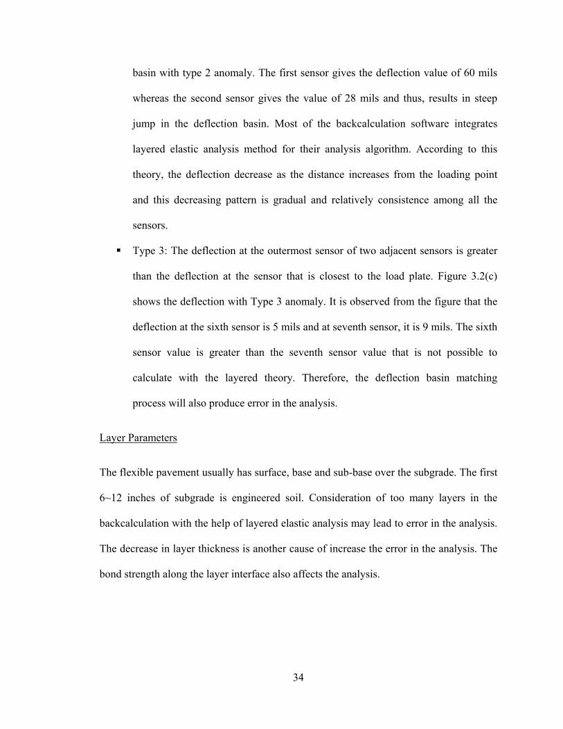
34
basin with type 2 anomaly. The first sensor gives the deflection value of 60 mils
whereas the second sensor gives the value of 28 mils and thus, results in steep
jump in the deflection basin. Most of the backcalculation software integrates
layered elastic analysis method for their analysis algorithm. According to this
theory, the deflection decrease as the distance increases from the loading point
and this decreasing pattern is gradual and relatively consistence among all the
sensors.
Type 3: The deflection at the outermost sensor of two adjacent sensors is greater
than the deflection at the sensor that is closest to the load plate. Figure 3.2(c)
shows the deflection with Type 3 anomaly. It is observed from the figure that the
deflection at the sixth sensor is 5 mils and at seventh sensor, it is 9 mils. The sixth
sensor value is greater than the seventh sensor value that is not possible to
calculate with the layered theory. Therefore, the deflection basin matching
process will also produce error in the analysis.
Layer Parameters
The flexible pavement usually has surface, base and sub-base over the subgrade. The first
6~12 inches of subgrade is engineered soil. Consideration of too many layers in the
backcalculation with the help of layered elastic analysis may lead to error in the analysis.
The decrease in layer thickness is another cause of increase the error in the analysis. The
bond strength along the layer interface also affects the analysis.

35
Temperature
Asphalt concrete is sensitive to the temperature. The strength of the surface course gets
reduced in the summer whereas the strength increases in winter. Therefore, temperature
plays an important role in the backcalculation. Usually, a temperature correction factor is
considered in a backcalculation software.
Seed Modulus
The initial set of modulus value that is selected for each layer may have an impact on the
analysis. The magnitude of the error depends on the iteration algorithm that is used by the
backcalculation software.
Modulus Ratio
The ratio of the modulus of elasticity of two adjacent layers. The analysis result is also
affected by the adjacent layer modulus ratio. If the ratio is significantly high this may
cause some error.
Underlying Rigid/Stiff Layer
The presence of the rigid/stiff layer at shallow depth causes a large error in the analysis if
that layer is not considered. The effect is pronounced whenever the depth is less than 10
ft (3.0 m). The stiff layer does not need to be bedrock, it can be a layer that is much
stiffer than the unbound layers above it. The depth to rigid layer has to be determined.
The layer at the deeper depth is responsible for the deflection of the sensor located farther
away from the loading point (Irwin 2000). The vertical deflection at the interface of the
subgrade-rigid layer is zero. Therefore, the radial distance where the vertical

36
displacement is zero is the depth to rigid layer (Irwin 2000). Prior to backcalculation of
the layer modulus, it is needed to determine this depth and thus, limit the thickness of the
subgrade. Figure 3.3 shows the method of rigid layer depth prediction. From Figure
3.3(a), it is observed that the deflection of the sensor is reduced with the distance away
from the load point and it is minimized at the farthest sensor. If the deflection basin is
extended after the last sensor point, it will be zero at some radial offset as indicated in
Figure 3.3(a). An arc of radius with same magnitude of the radial offset is then drawn.
The depth at which that arc intersects the vertical line is the depth to rigid layer. The
method of calculating this depth is shown in Figure 3.3(b). From the deflection basin
developed from the FWD, the inverse of the sensor radial offset is determined at different
locations. The displacements are then plotted against the inverse of the sensor radial
offset at different locations. A tangent is drawn along the initial straight part of that
curve. This tangent intersects x-axis at some point and this intercept is to be determined.
The inverse of this x- axis intercept is the depth to rigid layer.
Pavement Cracks
The one of the assumptions behind layered elastic analysis is that each and every layer is
infinite horizontally. Therefore, it does not consider any discontinuities in the layer of the
pavement. If the load plate is near to this crack, the analysis result may have some error.
3.3.3 Analysis
The collected data are investigated whether they satisfy the above mentioned
requirements or not. If the data set meets all the requirements, it can be used for the

37
analysis as described previously. The available commercial software or closed formed
solutions are able to backcalculate the layer moduli from the data.
3.3.4 Review of Backcalculated Modulus
The applicability of the backcalculated modulus from the analysis should be reviewed
according to the following requirements:
The error limit (percent difference between the measured and determined
deflections) will have to be within specified tolerance.
The values of the layer modulus will have to be investigated whether these are
reasonable or not.
The modulus value for the individual layer should be checked whether this often
hit the upper limit for each deflection basin.
The modulus value for the individual layer should be checked whether this often
hit the lower limit for each deflection basin.
The modulus ratios between the adjacent layers should be investigated whether
the values are realistic.
The backcalculated modulus will be acceptable if the values satisfy the above mentioned
requirements.
3.4 Backcalculation Software
A number of commercial software is for backcalculation as mentioned previously. This
study includes three software and one backcalculation algorithm from AASHTO 1993.
The details of the software are described below:

38
3.4.1 BAKFAA
BAKFAA is based on layered elastic analysis and employs a downhill multidimensional
simplex minimization method for the backcalculation of layer moduli (Press et al. 2007).
The downhill multidimensional simplex minimization method is suitable for finding the
minimum value of a function of more than one independent variable (Press et al. 2007).
BAKFAA calculates deflections at the specified points using the initial set of assumed
layer moduli or seed moduli. Error minimization process involves determination of sum
of the squares of differences between the FWD deflections and the deflections calculated
by layered elastic analysis. BAKFAA is written in Visual Basic platform. BAKFAA can
analyze a pavement having ten layers. However, BAKFAA cannot calculate the rigid
layer depth and it does not account for temperature effect in modulus calculation. In
BAKFAA, user has to assume the depth to rigid layer for the determination of subgrade
thickness.
3.4.2 MODULUS 6.0
MODULUS 6.0 uses the Waterways Experiment Station Linear Elastic Analysis
(WESLEA) method for forward calculation of moduli. WESLEA is developed based on
the multilayer elasto-static theory. A database of deflection basins is generated for
different modular ratio using WESLEA. It uses a pattern search technique to determine
the set of layer moduli which produces a deflection basin that best matches with the field
measured deflection (William 1999). It can analyze the pavement of maximum four
layers. The rigid layer depth prediction is one of the advantages of this software.
MODULUS assumes the radial distance to the point where the deflection is zero is

39
closely related to the rigid or stiff layer depth (Irwin 2002). MODULUS software also
accounts for the effect of temperature.
3.4.3 EVERCALC 5.0
EVERCALC 5.0 uses the WESLEA for the forward analysis. The forward analysis
involves the calculation of surface deflections at the specified radial offsets using
different combinations of initially assumed layer moduli. The calculated surface
deflections are then compared to the field measured deflections. For each combination of
layer moduli, the error between these calculated and measured moduli is determined. This
step is repeated several times until the error is minimized. This process is known as the
error minimization or optimization of solution. A modified Gauss-Newton algorithm is
used for error minimization. FWD data from a maximum of ten sensors can be used and
it can analyze twelve drops at each station. During the error minimization process, a trial
is stopped whenever one of the following conditions is satisfied first (Everseries User
Guide 2005):
- Deflection tolerance calculates deflection error between the field measured and the
calculated deflections using the following formula:
RMS %1n
w ww 100 3.1
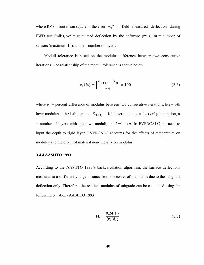
40
where RMS = root mean square of the error, w = field measured deflection during
FWD test (mils), w = calculated deflection by the software (mils), m = number of
sensors (maximum 10), and n = number of layers.
- Moduli tolerance is based on the modulus difference between two consecutive
iterations. The relationship of the moduli tolerance is shown below:
e %E E
E 100 3.2
where e = percent difference of modulus between two consecutive iterations, E = i-th
layer modulus at the k-th iteration, E = i-th layer modulus at the (k+1)-th iteration,
= number of layers with unknown moduli, and 1 to . In EVERCALC, no need to
input the depth to rigid layer. EVERCALC accounts for the effects of temperature on
modulus and the effect of material non-linearity on modulus.
3.4.4 AASHTO 1993
According to the AASHTO 1993’s backcalculation algorithm, the surface deflections
measured at a sufficiently large distance from the center of the load is due to the subgrade
deflection only. Therefore, the resilient modulus of subgrade can be calculated using the
following equation (AASHTO 1993):
M0.24 Pr d 3.3

41
where M backcalculated subgrade resilient modulus (psi), P applied load (lb), and
d deflection at a distance r (in) from the center of the load (in). The value of r is
calculated using the following relationship (AASHTO 1993):
0.7 3.4
where M backcalculated subgrade resilient modulus (psi), a radius of loading plate
(in), D total thickness of pavement layers above the subgrade (in), and E effective
modulus of all pavement layers above the subgrade (psi). The effective modulus (E ) of
all the pavement layers above the subgrade is related to the backcalculated subgrade
modulus through the following relationship (AASHTO 1993):
M dq a 1.5
1
1 Da
EM
1 1
1 Da
EM
3.5
where d deflection measured at the center of the load plate (in), q load plate
pressure (psi), a load plate radius (in), and D total thickness of pavement layers
above the subgrade (in). In AASHTO 1993 procedure, at first the Mr is calculated by an
assumed radial offset r using the Equation (3.3). Next Equation (3.5) is used to calculate
Ep from the known Mr and assumed r value. Next a new r value is calculated using the

42
known Mr and Ep in Equation (3.4). This process is repeated until this new r value
matches with the initially assumed r value. To avoid this iterative process, the New
Mexico Department of Transportation (NMDOT) uses the surface deflection at fifth
sensor in Equation (3.3) to determine the subgrade modulus.
3.5 Factors Affecting Backcalculated Modulus
3.5.1 Loading
The load magnitude and the duration play a significant role in the measurement of FWD
deflection. The FWD device is designed with the purpose to determine the pavement
response due to the traffic load. The traffic load may be either from vehicle or aircraft.
So, the most important issue here is the load should be same as that from the traffic and
the loading duration should be compatible with the real field situation. The nonlinear or
the stress-sensitive behavior of the pavement material is the difficulty for the load to be
proportional to the deflection. Generally, the pavement is subjected to different
magnitudes of load. So, if the test is done with a certain amount of load and then it is
needed to estimate the deflection for the heavier load, the deflection should be
extrapolated. For the remedy of this situation, a number of correlations or regression
equations are developed to relate the deflection from the lighter load to that from the
higher load. But, due to the construction practices and the environmental conditions,
these correlations may differ from each other for a same pavement.
3.5.2 Climate
Climate has a greater influence on the FWD deflection measurement. First, the
temperature affects the deflections in both flexible and rigid pavement. In case of flexible
43
pavement, the surface is made of asphalt concrete and it is a visco-elastic material. So,
temperature is the most important factor in load-deflection criterion for visco-elastic
material. In higher temperature, the pavement shows higher deflection under a given load
than that in lower temperature. Thus, flexible pavement is affected by the temperature
variation during deflection measurement. For rigid pavement, the deflection is affected
by the thermal gradient near the zone joint and cracks. The higher temperature causes the
pavement to expand and thus, it leads to the tightening of the joint. As a consequence, the
deflection will be less. The deflection can change due to the curling of the pavement. At
the lower temperature, the surface of the pavement gets contracted and it results the
higher deflection at the edge and corner.
The deflection is also influenced by the seasons. Four distinguished periods are marked in
colder region. The period of deep frost occurs during the winter season and the pavement
is the strongest at this time. The deflection will be lowest during this period. The frost
begins to disappear when the spring thaw starts and the deflection gets higher. In early
summer, the excess free water from the melting frost leaves the pavement system and
thus, the deflection decreases. The period of slow strength recovery extends from late
summer to fall when the deflection levels off slowly as the water content slowly
decreases. The deflection follows a sine curve in the region where the pavement does not
experience any freeze-thaw cycle. In this situation, the deflection is high in wet season
when the moisture content is high. In dry areas, the higher deflection is observed in
summer whenever the pavement surface softens due to high temperature.

44
3.5.3 Pavement Condition
The effect of pavement condition on the deflection measurement is significant. During
the measurement of deflection in flexible pavement, the reading is high if that pavement
has the distress like cracking or rutting. In rigid pavement, the void underneath the slab
causes higher deflection value. The deflection can also be affected in this pavement by
the load transfer deficiency due to lack of proper load transfer device along the joint.
Deflections measured near or over a culvert show higher deflection than the expected
value. The deflections of the pavement surface in cut or fill section may be deviated from
exact value.
3.6 Backcalculation in Airport Pavement Evaluation
This study is mainly based on the evaluation of the airport pavement strength in New
Mexico. As a part of the evaluation methods, FWD data analysis is the center of focus in
this literature. FWD data are collected from the airports according to the FAA guideline
and thus, a number of data sets are populated for each airport pavement. The tests were
carried out at various points all through the pavement and figure 3.4 shows the
generalized plan of the FWD test. To cover the whole region of pavement, six test lines
were selected for the evaluation. The test stations along each and every line are
mentioned in the Table 3.1. At each station, three load levels of 9, 12, and 16 kips were
applied. And at each load level the test is performed twice. For the analysis of the FWD
data, the thickness of the individual layer is to be known. Asphalt coring and soil
sampling from the pavement was the part of this project. The coring was done at every
1000 ft. interval as shown in the Figure 3.5. To get a clear view of the coring strategy,

45
this figure shows only three coring points as an example. The FWD was done at different
intervals including 200, 400, and 600 ft. that results a number of the data sets inside this
coring interval. Then, for the analysis thicknesses of the layers needed to be assumed
based on the adjacent coring information. The 1000 ft. segment of the pavement is
considered with the 500 ft. length of the pavement on either side of the coring point. The
thicknesses of the surface and base course are thus collected from this pavement segment.
Now, the subgrade thickness is determined by subtracting the thicknesses of the surface
and base from the depth to rigid layer. The coring also gives the information about the
material properties of the layer. The FWD data is then analyzed with the available
information to determine the pavement layer modulus. For the analysis, the above
mentioned backcalculation software are used.
3.7 Summary
The above discussions in this chapter can be summarized as follows:
Prior to the backcalculation process, the data relevant to the test and the pavement
have to be collected. The data includes the FWD test load, pavement surface
deflections due to the test load, and pavement surface temperature.
From the bore log, the information about the number of layers and their individual
thickness as well as the material comprising the layer have to be collected.
The test data and bore log information have to be checked carefully whether there
are any irregularities or potential problem involved in the data according to FAA
guideline.

46
After having all the data with necessary checks, the layer moduli of pavement
have to be backcalculated according to the steps described earlier.
The backcalculated layer moduli should be reviewed for their acceptability, i.e.
whether the value of the backcalculated modulus be reasonable for the individual
layer, in the pavement strength evaluation.

47
Table 3.1: FWD test plan
Test Line Distance from Centerline Test Interval 1 & 4 5 feet @200 ft. c/c 2 & 5 20 feet @400 ft. c/c 3 & 6 40 feet @600 ft. c/c
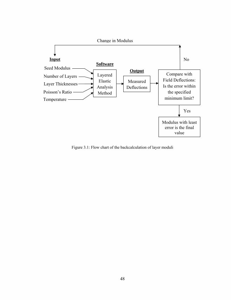
48
Figure 3.1: Flow chart of the backcalculation of layer moduli
Input
Layered Elastic
Analysis Method
Software
Modulus with least error is the final
value
Compare with Field Deflections: Is the error within
the specified minimum limit?
No
Change in Modulus
Yes
Measured Deflections
Output
Layer Thicknesses
Temperature Poisson’s Ratio
Number of Layers
Seed Modulus

49
(a) Type 1
(b) Type 2
(c) Type 3
Figure 3.2: Different types of anomalies in deflection type
05
101520253035
0 10 20 30 40 50 60D
ispl
acem
ent (
mils
)Sensor offset (inches)
010203040506070
0 10 20 30 40 50 60
Dis
plac
emen
t (m
ils)
Sensor offset (inches)
05
10152025303540
0 10 20 30 40 50 60
Dis
plac
emen
t (m
ils)
Sensor offset (inches)

50
(a) Influence of the shape of deflection basin on the rigid layer depth prediction
(b) Determination of the depth of the rigid layer
Figure 3.3: Rigid layer depth determination
0
5
10
15
20
25
30
35
0 0.05 0.1 0.15
Dis
plac
emen
t (m
ils)
1/r (1/inches)
Surface
Base
Dep
th to
Rig
id L
ayer
Subgrade
Rigid Layer
Load
Rigid layer depth = 1/x-intercept
Tangent with the initial part of the curve
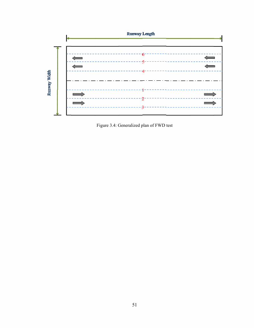
Figure 3.4: G
51
Generalized p
plan of FWD test
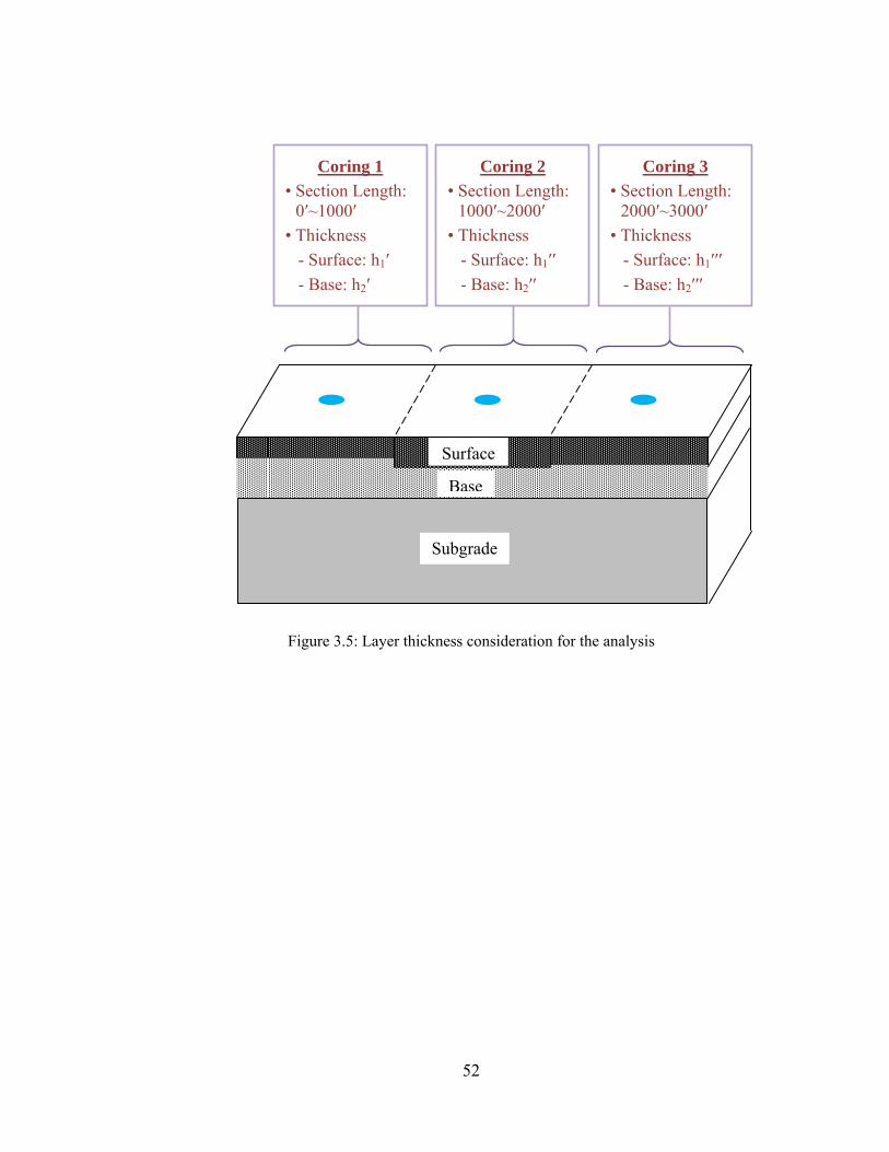
52
Figure 3.5: Layer thickness consideration for the analysis
Surface
Base
Subgrade
Coring 1 • Section Length:
0′~1000′ • Thickness - Surface: h1′ - Base: h2′
Coring 2 • Section Length:
1000′~2000′ • Thickness - Surface: h1′′ - Base: h2′′
Coring 3 • Section Length:
2000′~3000′ • Thickness - Surface: h1′′′ - Base: h2′′′

53
CHAPTER 4
ACCURACY AND CONSISTENCY
4.1 Introduction
Backcalculated moduli are used in important applications such as pavement design,
strength evaluation, and overlay thickness design. It is important to know the accuracy
and consistency of the analysis results obtained from backcalculation software. Most of
backcalculation software does not produce the same layer moduli from inputs at same test
point. The outputs depend on the seed or initial modulus required to run the
backcalculation software. Also, the outputs vary depending on the type of the error
minimization algorithm used in a specific software. There is a need for a study to select
the most accurate and consistent software for the backcalculation of layer modulus to
process FWD data, which is done in this chapter.
4.2 Objectives
The objectives of this study are mentioned below:
Examine the consistency of backcalculation software when processing FWD data
of a single location using three different load levels: 9 kip, 12 kip, and 16 kip.
Evaluate the accuracy of backcalculation software by comparing laboratory
resilient modulus to the backcalculated modulus. In addition, compare laboratory
tensile strength of asphalt concrete to field tensile strength obtained using the
backcalculated moduli as inputs to a multilayer elastic analysis. Here, software
accuracy is investigated based on the tensile strength of an asphalt concrete.

54
4.3 Study Approach
In this study, asphalt cores, aggregates, and soils were collected from locations where
FWD tests were conducted as a first step. Three FWD tests were conducted at each
location using 9 kip, 12 kip, and 16 kip loads. The consistency of the software is
evaluated through the frequency plot of the modulus backcalculated by each software. A
software is considered consistent when the frequency curves of the backcalculated
modulus at three loads overlap each other. To further investigate the consistency, the
coefficient of variation (CV) of backcalculated moduli in response to the load increments
is utilized. The higher the value of CV, the lower is the consistency. Based on this, the
most consistent software is the one that shows the least CV of backcalculated moduli at
the specified load levels. To verify the accuracy, software outputs are compared to the
laboratory test results. Laboratory test results are considered to be the representative of
the field condition. Laboratory test includes the resilient modulus and indirect tensile
strength of asphalt concrete. Also, the tensile stress at the bottom of the surface AC layer
is determined by KENLAYER, which is a multi-layer elastic program (Huang 2004). To
further investigate the accuracy, the backcalculated subgrade modulus is compared to
subgrade resilient modulus obtained from California Bearing Ratio (CBR). The most
suitable backcalculation software is the one that has high accuracy and consistency
among three.
4.4 Data Collection and Testing Plan
The FWD tests were conducted at seven runways in New Mexico. They are runway 4-22
of Double Eagle II Airport, runway 12-30 0f Sierra Blanca Regional Airport, runway 2-

55
20 and 7-25 of Raton Municipal Airport, runway 8-26 of Las Cruces International
Airport, runway 8-26 of Moriarty Airport and runway 8-26 of Silver City Airport. All of
these runways had surface course consists of asphalt concrete. Thirty nine bore holes
were drilled in those runways to collect asphalt core, aggregates, and soil beneath.
Drilling was performed at locations where FWD tests were conducted. In the FWD
testing plan, each location was tested at three load levels: 9, 12, and 16 kips. At each load
level, two replicate FWD tests were performed.
4.4.1 FWD Testing
FWD test was performed by JILS FWD 20T. In this equipment, an impulse load was
generated on the pavement surface by dropping a weight on a circular plate of 12 in.
diameter from a height of 1.64 ft using a spring-mass system. The duration of the load
was 20-34 milliseconds. The steel plate comes to a smooth contact with the surface of the
pavement by the use of a rubber pad. Pavement deflections are measured by seven
geophones resting longitudinally on the surface. Under load, the pavement surface
deflects vertically downward forming a deflection basin. Seven geophones were used at
different radial offset from the load. The distances of the geophones from the center of
the loading plate are 0, 8, 12, 18, 24, 36, and 60 inches. As motioned previously, the
magnitudes of the load were varied at three load levels of 9, 12, and 16 kips. For each
load, two replicate tests were performed at a single test point or location. FWD test was
carried out in accordance with the ASTM D 4694-96.

56
4.4.2 Asphalt Coring and Soil Sampling in the Field
Before drilling, a preliminary drilling or coring plan was designed to cover mostly the
center part of the entire runway. This was not done according to the FAA guideline,
which requires coring at every 200 ft location. Because of time and funding limitations,
coring performed at a spacing of 1000 ft.
Figure 4.1(a) shows an example of coring locations at Raton Municipal Airport in New
Mexico. This airport has two runways namely, runway 7-25 and runway 2-20. Drilling
was carried out at five locations in runway 7-25 and six locations in runway 2-20. Some
drill locations are shown on taxiway. A detailed coring plan of runway 2-20 is shown in
Figure 4.1(b). The starting point of this runway is at 36-44.05N latitude and 104-30.67W
longitude. The elevation is at 6332.1 ft. The first drill location is 1000 ft. from the start
point, and the subsequent drilling or coring points are at 1000 ft. spacing, alternately on
both sides of the centerline. It can be seen that core or drill no. 9, 11, and 13 are located
29, 13, and 17 ft. respectively from the centerline on its left. Again, core hole or drill no.
10, 12, and 14 are located 17 ft, 27.5 ft, and 13.5 ft. from the centerline on its right. The
end point is at 36-44.91N latitude and 104-29.94W longitude. The elevation is at 6352.4
ft. At each drill location, four coring were made to collect four asphalt samples. The soil
and aggregate underneath the asphalt surface was collected.
Borehole information for core location number 9 is shown in Table 4.1. A brief summary
of the coring location, layer thickness, and layer properties were documented during field
testing and are presented in Table 4.1. The first column shows the coring location from
the start point and the distances are in ft. Samples were collected in sacks. The second
column shows the identification number of sack. The third column shows the
57
identification number of hole. The asphalt cores, base, and subgrade materials were
collected from each of these holes. At each hole, the layers were identified by A, B, C,
and D. If different soils encountered, they were collected in different bags and identified
with letters such as C, D, E, and F. The fifth and sixth columns show the layer
information. The seventh column shows the source of the materials such as the surface,
base, or subgrade. The soil type information was recorded based on field or visual
identification.
Table 4.2 presents the summary of the number of cores, layer type and thickness, and
subgrade soil classification form laboratory testing. For example, the subgrade soils of
runway 12-30 at Sierra Blanca Regional Airport and runway 2-20 at Raton Municipal
Airport are clayey gravel, whereas subgrade soils of runway 7-25 at Raton Municipal
Airport varies from clayey sand to gravel with sand and silt. The subgrade of the rest of
the runways is silty sand. The thickness of the surface course varies from 2.25 inch to
9.75 inch, with a mean of 5.77 inch and standard deviation of 1.86 inch. The base course
thickness varies from 5 inch to 15 inch, with a mean of 9.67 inch and standard deviation
of 3.1 inch.
4.5 Laboratory Testing
4.5.1 Resilient Modulus of Asphalt Concrete
Asphalt cores were tested to determine the resilient modulus using an indirect tensile
resilient modulus testing apparatus from Retsina Co. at the Pavement Laboratory at the
University of New Mexico. Many asphalt samples were found to have thickness less than
4 inch after extraction, although the total thickness of the surface layer was more than 6

58
inch. It is possible that several thin layers of asphalt were laid to get to the total thickness
because of compaction limitation. These thin asphalt cores are not suitable for cylindrical
or axial test. Therefore, indirect tension modulus test was selected for these samples
(ASTM D 4123). In indirect resilient modulus test, asphalt core sample was subjected to
a repeated load of 30 lb along its diametric axis as shown in Figure 4.2(a). The thickness
of the core was measured at four points which are 90º apart and the average thickness
was determined. All the tests were carried out at room temperature (23.2±1ºC) and three
replicate tests conducted on each sample. The repeated load and the recoverable
horizontal deformation were recorded. The resilient modulus is calculated using the
following formula (ASTM D 4123):
0.27 4.1
where, M = resilient modulus (psi), P = repeated load (lbs), δ = total recoverable
horizontal deformation (inch), t = specimen thickness (inch), and ν = Poisson’s ratio.
Poisson’s ratio for asphalt concrete was assumed to be 0.35 (Huang 2004).
Table 4.3 shows the resilient modulus of asphalt concrete cores from seven runways. It
can be seen that, the resilient modulus of runway 4-22 of Double Eagle II airport varies
from 230.1 to 285.3 ksi, and for runway 12-30 of Sierra Blanca Regional airport is within
the range from 225.3 to 270.9 ksi. The maximum value of resilient modulus is observed
285.3 ksi at runway 4-22 of Double Eagle II airport and the minimum of 202.3 ksi at
runway 7-25 of Raton Municipal Airport. The modulus values are mostly around 250 ksi
and below 300 ksi. Generally resilient modulus of new asphalt pavements varies from
500 to 2000 ksi (Tarefder et al. 2007). Based on that, it can be suggested that the runway

59
pavements have lost their modulus values at least 50%. In other words, it can be roughly
said that these runway asphalt concretes’ structural capacity reduced 50% or half of their
design life.
4.5.2 Indirect Tensile Strength of Asphalt Concrete
Indirect Tensile Strength (ITS) tests of the asphalt cores were conducted using a
Humboldt device as shown in Figure 4.2(b). In this equipment, asphalt sample was
loaded across its vertical diametric plane with a loading rate of 50 mm/minute (ASTM D
4123-82). Load-displacement data was collected using LabVIEW software. All the tests
were carried out at room temperature (23.2±1ºC). The maximum load at failure was
recorded and the ITS is calculated using the following formula:
2 4.2
where, S = indirect tensile strength (psi), P = maximum load (lb), t = core length (inch),
and D = core diameter (inch). The values of the ITS are shown in Table 4.3. For example,
the ITS of AC from Runway 4-22 of Double Eagle II airport varies from 230.4 to 249.8
psi and for runway 12-30 of Sierra Blanca Regional airport varies from 213.4 to 306.0
psi. Most of the runways have shown an ITS value above 200 psi, which is a bit high,
compared to the roadway pavements’ ITS values. ITS values are often related to the low
temperature cracking of asphalt pavement (MEPDG 2004).

60
4.6 Consistency of the Software
4.6.1 Frequency Plot of Mr
As mentioned previously, consistency of software is analyzed by comparing software
outputs from three sets of data varied for three load levels at a single location in the field.
A frequency plot of these backcalculated moduli (Mr) of cores from 39 locations are
performed at 3 load levels. If the frequency plots for these 3 load levels overlap on each
other, it can be said that there is little to no variation in the backcalculated modulus due to
those loads. In other words, the software is consistent. The frequency distribution
includes a total of seventy eight data points (39 cores x 2 replicate tests).
Figure 4.3 is plotted to examine the consistency of the software for the surface layer.
From Figure 4.3(a), it is observed that the frequency distributions of the backcalculated
surface modulus from MODULUS at the specified loads overlap on each other over the
range 200-750 ksi. After that, the lines deviate slightly and converge at 2000 ksi. The
frequency distribution plots of EVERCALC, shown in Figure 4.3(b), overlap in the range
of 200-450 ksi. These lines then start deviating from each other and converge again at
1500 ksi. The frequency distributions of BAKFAA shown in Figure 4.3(c) do not overlap
over the modulus variation. From these plots, it can be said that the MODULUS is the
most consistent for the backcalculation of surface modulus.
The aforementioned frequency plots are shown in Figure 4.4 and 4.5 for the base and
subgrade layer, respectively. Figure 4.4(a) shows that the frequency distributions from
EVERCALC start deviating from each other after 30 ksi. These lines do not overlap at
any the range of modulus variation except at 175 ksi. At a base modulus value of 50 ksi,

61
the frequencies of 9, 12, and 16 kip load lines are 38, 31, and 33, respectively. Whereas at
Mr =100 ksi, the frequencies are 13, 22, and 17 units. From Figure 4.4(b), it can be seen
that the frequency distributions from EVERCALC overlap at 12 and 16 kip loads for
almost all the modulus variation except at Mr =100 ksi. The frequency distribution of 9
kip shows the maximum deviation from those of 12 and 16 kip at Mr = 50 ksi. The
magnitudes of these frequencies are 13, 8 and 8, respectively. From Figure 4.4(c), it is
clearly evident that the deviations in the frequency distributions of the base modulus from
BAKFAA are noteworthy. The lines do not overlap over the modulus variations.
Therefore, it can be said that EVERCALC is the most consistent among three for base
modulus calculation.
Frequency plots of subgrade are shown in Figure 4.5. It can be seen that all the software
are nearly consistent except MODULUS. The large deviations in the frequency
distributions from MODULUS software are observed at the modulus values of 10, 15,
and 20 ksi. To that end, it can be concluded that MODULUS is not consistent software
for the subgrade modulus.
4.6.2 Frequency Plot of CV of Mr
To further examine the consistency of backcalculation software, the coefficient of
variation (CV) of the layer moduli is determined at each test point using the following
formula:
% 100 4.3

62
where, = standard deviation, and µ = mean of the backcalculated modulus using three
different loads. Table 4.4 shows the CV of the backcalculated moduli obtained from three
software. Due to space limitation, data of runway 8-26 of Silver City Airport is shown
and discussed here. From Table 4.4, it is evident that the CV of surface modulus from
MODULUS is the smallest. Both EVERCALC and BAKFAA show higher CV values at
this location or data point. For base and subgrade modulus, clearly EVERCALC has the
smallest CV value. However, this is only for this single data point at Silver City Airport.
To get a general trend of the consistency of the analysis methods, frequency distribution
of the CV for all data points is plotted as described in the following paragraph.
In the frequency vs. CV plot, if the peak of the distribution leans towards the lower
values of CV that indicates the majority of the data have low CV. That means that the
variation in that data set is small. On the other hand, if the peak of the distribution leans
towards a high value of CV, it indicates that the majority of the test data have low CV. It
means that the variation is high in that data set. Therefore, the most consistent software is
the one that shows the peak value of frequency at smaller CV value. But, this is not the
only criterion for a software to be considered the most consistent. The shape of the
frequency distribution curve must be investigated to observe the amount of deviation that
an analysis shows.
Surface Modulus
The percentage frequency distributions of the CV of backcalculated surface modulus are
plotted in Figure 4.6(a). At CV of 0, the frequencies of MODULUS, EVERCALC, and
BAKFAA are 60, 54, and 0, respectively. It is observed that the frequency of
EVERCALC decreases more rapidly than that of MODULUS after the peak value,

63
whereas BAKFAA still increases. BAKFAA shows the peak frequency 19 at a CV value
of 10. It also shows the frequencies of 8 and 9 at the CV values of 30 and 50,
respectively. Therefore, the backcalculated surface modulus from BAKFAA is not very
consistent. MODULUS and EVERCALC analysis results are reasonably consistent
though both of them show high variations with at some points.
Base Modulus
Figure 4.6(b) shows the percentage frequency distribution of the CV of the
backcalculated base modulus from three software. The percentage frequency of
MODULUS is 36 at the CV of 0, whereas that of the EVERCALC is 62, and BAKFAA
is 18. It means that the deviation in the analysis results is lower from EVERCALC than
that from MODULUS and BAKFAA. The CV value from EVERCALC converges
smoothly to the zero soon after the peak value and this rate is more rapid than
MODULUS. The fluctuation in CV value from BAKFAA is high. It can be said that
EVERCALC is the most consistent for the backcalculation of base modulus.
Subgrade Modulus
Figure 4.6(c) shows the frequency distribution of the CV of the backcalculated subgrade
moduli from three software as well as from AASHTO 1993. At the CV of 0, the
frequency of EVERCALC is 31 whereas that of the other software is zero. It can be seen
that the peak percentage frequencies of MODULUS, EVERCALC, BAKFAA, and
AASHTO 1993 are 13, 47, 26 and 82, respectively at the CV of 5. Above the CV value of
5, the frequency values from all software decreases gradually except MODULUS
software. MODULUS has attained at the peak frequency 47 at a CV value of 10. For

64
EVERCALC and AASHTO 1993, the shape of the curves are almost flat and parallel to
the horizontal axis compared to others. It means the CV fluctuation is smaller in
EVERCALC and AASHTO 1993 than that in MODULUS and BAKFAA. So, it can be
said that EVERCALC and AASHTO 1993 can backcalculate the subgrade modulus more
consistently than the MODULUS and BAKFAA software.
4.7 Accuracy of the Software
Software accuracy will be examined based on the rule as follows: a software is accurate if
it produces modulus values that match the modulus values measured in the laboratory.
4.7.1 Backcalculated vs. Measured Modulus of Asphalt Concrete
Three out of four cores collected from each of the 39 drilling locations were tested for
modulus in the laboratory. The average of the three core values is reported to be
representative value of modulus for a single drilling location. In this section, average
resilient modulus value of asphalt concrete is compared to the backcalculated FWD
modulus from 9, 12, and 16 kip load FWD tests data.
Based on 9 kip load
The accuracy of the backcalculated modulus is examined by plotting backcalculated
modulus against laboratory modulus as shown in Figure 4.7. The accuracy is indicated by
a line of equality (on which backcalculated value is equal to the measured value). If the
data points are close to or on the line of equality, backcalculated surface modulus is
accurate. From Figures 4.7(a), 4.7(b), and 4.7(c), it can be seen that most of the data
points from EVERCALC are close to the line of equality. That is, EVERCALC shows the

65
majority of the data fall near to the line of equality among the three software. Therefore it
can said that at 9 kip load the EVERCALC software produces surface modulus that are
close to the laboratory resilient modulus.
Based on 12 kip load
Figure 4.8(a) compares these software accuracy at 12 kip load. It can be seen that
majority of data from EVERCALC backcalculation is near to the line of equality. The
backcalculated surface moduli from the other MODULUS and BAKFAA software are
scattered over a wide range and away from the line of equality. Therefore, it can be
concluded that EVERCALC analysis results are more accurate than other software.
Based on 16 kip load
Figure 4.8(b) is plotted to check the accuracy of these software at 16 kip load. Again, the
data points near to the line of equality are from EVERCALC software. Therefore, again
at 16 kip load EVERCALC is more accurate than MODULUS and BAKFAA software.
4.7.2 Backcalculated vs. Measured Modulus of Subgrade
In this section software accuracy is examined by comparing backcalculated subgrade
modulus to measured modulus. As mentioned previously, resilient modulus of subgrade
soil was not obtained directly by conducting laboratory testing. Soils index property
testing and classification were performed in the laboratory. Modulus value was then
obtained from existing relationships of soil index properties and resilient modulus of soil
and it is termed as soils “laboratory” modulus in this paper. Several authors including
Witczak et al. (1995) mentioned a number of empirical relations between resilient
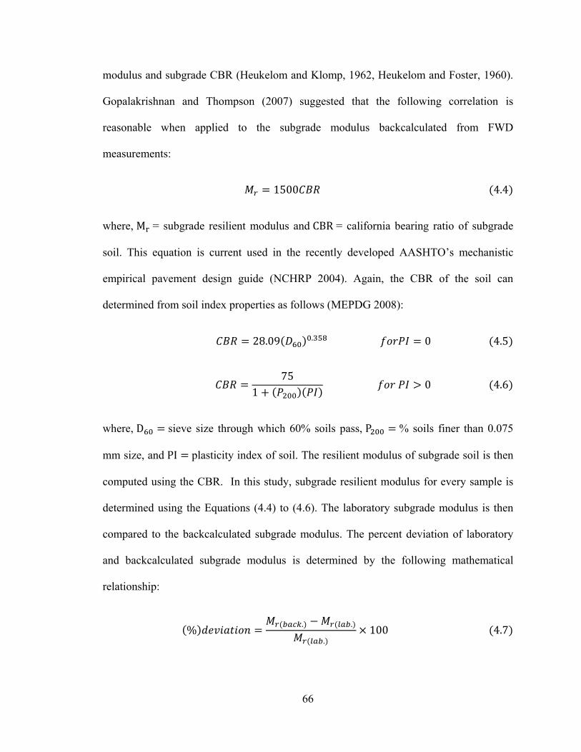
66
modulus and subgrade CBR (Heukelom and Klomp, 1962, Heukelom and Foster, 1960).
Gopalakrishnan and Thompson (2007) suggested that the following correlation is
reasonable when applied to the subgrade modulus backcalculated from FWD
measurements:
1500 4.4
where, M = subgrade resilient modulus and CBR = california bearing ratio of subgrade
soil. This equation is current used in the recently developed AASHTO’s mechanistic
empirical pavement design guide (NCHRP 2004). Again, the CBR of the soil can
determined from soil index properties as follows (MEPDG 2008):
28.09 . 0 4.5
751 0 4.6
where, D sieve size through which 60% soils pass, P % soils finer than 0.075
mm size, and PI plasticity index of soil. The resilient modulus of subgrade soil is then
computed using the CBR. In this study, subgrade resilient modulus for every sample is
determined using the Equations (4.4) to (4.6). The laboratory subgrade modulus is then
compared to the backcalculated subgrade modulus. The percent deviation of laboratory
and backcalculated subgrade modulus is determined by the following mathematical
relationship:
% . .
.100 4.7

67
where, M . = backcalculated subgrade resilient modulus, and M = laboratory
subgrade resilient modulus from correlation equations.
Figures 4.9(a), 4.9(b), and 4.9(c) are plotted to investigate the accuracy of the software
based on the subgrade modulus due to load levels 9, 12, and 16 kips. In these figures,
laboratory subgrade modulus is plotted on the horizontal axis and backcalculated
modulus is plotted on the vertical axis. The line of equality goes through the points at
which both the laboratory and backcalculated modulus are same. A software is
considered to be the most accurate when most of the data points are on the line of
equality. Figures 4.9(a), 4.9(b), and 4.9(c) show that most of the backcalculated moduli
from the aforementioned software are below 40 ksi along. From Figure 4.9(a), for 9 kip
load, only a few data from EVERCALC is on or near to the line of equality. So,
EVERCALC is more accurate than other software for 9 kip load application. Figure
4.9(b) represents the accuracy of the software for the backcalculation of subgrade
modulus using 12 kip FWD test load. Again the backcalculated moduli from
EVERCALC are near to the line of equality. It means that EVERCALC is still accurate
for 12 kip load data analysis. Similar trend can be observed from Figure 4.9(c).
Therefore, this study concludes that EVERCALC software is the most accurate in the
backcalculation of subgrade modulus.
4.8 Backcalculated vs. Measured Tensile Strength of Asphalt Concrete
It is known that tensile stress develops at the bottom of the asphalt layer, particularly in
thin pavements, under vertical loads. This is schematically shown in Figure 4.10.
Airports, as well as roadway pavements are comprised of three layers surface, base, and

68
subgrade underlain by a rigid layer. Each layer can be assigned a modulus of elasticity
(En), Poisson’s ratio (υn), and thickness (hn), where n is the layer number. As the FWD
ball is dropped on the runway pavement surface, the bottom of the asphalt or surface
layer undergoes through tension. In this study, KENLAYER, a layered elastic analysis
software, is employed to determine the tensile stress at the bottom of the surface asphalt
layer (Huang 2004). KENLAYER program requires inputs of modulus of each layer. So
as first step, backcalculation software were employed to determine the layer modulus and
then they are given as inputs to KENLAYER program. As the KENLAYER inputs came
from the backcaculated moduli, the tensile stress (KENLAYER output) is termed as
“backcalculated tensile stress” in this paper. The backcalculated tensile stress is then
compared to the laboratory indirect tensile stress or strength for accuracy analysis.
In this study, only 9 kip load is used in KENLAYER analysis. Figure 4.11 shows the
backcalculateed versus laboratory tensile strength. Figure 4.11(a) shows laboratory
tensile strength in horizontal axis and backcalculated tensile stress from MODULUS
software in the vertical axis. Here again a line of equality is drawn to set a reference from
comparison. The accuracy of the backcalculated value to the laboratory strength value
can be evaluated by how close these data points from this line. The backcalculated
tensile strength is equal to the laboratory value whenever a point lies on this line of
equality. Figure 4.11(b) is plotted for EVERCALC and Figure 4.11(c) for BAKFAA
software. From these figures, it is observed that the tensile stress calculated for
EVERCALC modulus values are close to the reference line. Therefore, from the accuracy
point of view, EVERCALC is the most appropriate software among the software studied
herein.

69
4.9 Conclusion
This chapter can be concluded as follows:
The consistency of FWD backcalculation software is evaluated using frequency
distributions of the backcalculated moduli and CV of moduli from an identical
location tested at three levels of FWD loads. For surface modulus, variation in
modulus and CV of EVERCALC software are slightly higher than those of
MODULUS software. The base modulus variation is the least in EVERCALC.
For subgrade modulus, EVERCALC is more consistent than BAKFAA and
MODULUS. Overall, the variation is highest in BAKFAA, and MODULUS
ranked second. EVERCALC is the most consistent backcalculation software for
determining runway pavement layer moduli.
The accuracy of the backcalculated surface modulus is examined by comparing
backcalculated modulus to the laboratory resilient modulus. It is shown that
EVERCALC produces modulus values closer to the laboratory resilient modulus
compared to MODULUS and BAKFAA software.
Based on the comparison of the backcalculated tensile strength to the laboratory
indirect tensile strength of the asphalt core, it is shown that EVERCALC is more
appropriate than MODULUS and BAKFAA software.
Based on the comparison of the backcalculated subgrade modulus to the
laboratory subgrade modulus, it is evident that backcalculated subgrade modulus
from EVERCALC is more close to the laboratory value than that from
MODULUS and BAKFAA software.

70
Overall, EVERCALC has the highest accuracy and consistency compared to the
MODULUS and BAKFAA software.
Stress dependency of the soil and aggregate is out of scope of this study for the
consistency analysis. Farther study is recommended to observe the effect of stress
dependent behavior of the soil and aggregate on the consistency of the analysis by
the software.

71
Table 4.1: Borehole information in Runway 2-20 (Raton municipal airport)
Subgrade Borrow Surfacing Filler Thru Pavement Source Location: Runway 2-20
Lab No.
Sack No. Hole & Sample Number
Depth Material Type
Remarks & Material
Identification From To
Mile Post:
1000 ft.
Rt. or Lt.
C/L 348in.
Distress
(1) Transverse (2) Longitudinal (3) Alligator (4) Pothole (5) Bleeding (6) Raveling (7) Polished Aggregate (8) Reflective (9) Blade Path (10) Rutting (11) Pumping
N/S Hole#9 A 0.0 8.0
Asphalt Concrete
Location measured in ft. north of Runway 02 threshold
G98
B 8.0 15.0
Base Course
Asphalt treated
N44
C 15.0 33.0 Subgrade
Gravely gray-green sandy clay (plastic clay fraction); angular 1/2’’-1 1/2’’ lithic arkose
G61
D 33.0 40.0 Subgrade
Dark gray-green sandy clay with rust and black sandy mottles
N72
E 40.0 53.0 Subgrade
Dark sandy clay (moist, moderate ribbon)
G22
F 53.0 71.0 Subgrade
Light tan sandy clay (moist, moderate ribbon, adhesive)

72
Table 4.2: Thicknesses of the Layers and Subgrade Soil Classification
Runway Layer No. of Cores
1 2 3 4 5 6 7
RW 4-22 (DE II)
Surface 2.5 2.5 2.5 2.5 2.5 2.25 - Base 6.5 5.5 6.5 5.5 6.5 6.75 -
Subgrade SP-SM SW-SM SW-SM SP-SM SW-SM SP-SM -
RW 12-30 (SBR)
Surface 5.0 5.0 5.0 5.0 5.0 - - Base 13.0 13.0 13.0 14.0 13.0 - -
Subgrade GW GW SW SW SW - -
RW 2-20 (RMA)
Surface 8.0 8.0 5.0 7.0 6.0 7.0 - Base 7.0 6.0 6.0 8.0 9.0 5.0 -
Subgrade GP-GC GW-GC SC GP GP-GC GW-GC -
RW 7-25 (RMA)
Surface 9.0 6.0 7.0 8.0 - - - Base 12.0 14.0 15.0 14.0 - - -
Subgrade SW SC GW GP-GM
- - -
RW 8-26 (LCIA)
Surface 5.0 4.5 4.5 6.0 - - - Base 11.0 10.0 9.0 8.0 - - -
Subgrade SP-SM SP-SM SP-SM SP-SM - - -
RW 8-26 (MA)
Surface 6.5 6.5 6.5 6.0 6.0 6.0 6.0 Base 0.0 0.0 0.0 0.0 0.0 0.0 0.0
Subgrade SP-SM SP-SM SM SM SM SM SM
RW 8-26 (SCA)
Surface 6.0 7.0 6.0 7.5 8.0 6.5 9.75 Base 11.0 8.0 9.0 8.5 12.0 10.5 13.25
Subgrade SP-SC SW-SC SP-SM SP SP-SM SW SM Note: Thicknesses of the layers are in ‘inches’

73
Table 4.3: Resilient Modulus and Indirect Tensile Strength of Asphalt Core
Runway Test Core number
Mean 1 2 3 4 5 6 7
RW 4-22 (DE II)
Mr 264.7 274.0 285.3 265.0 230.1 259.6 ― 263.1 ITS 242.3 246.7 249.8 230.4 238.2 239.4 ― 241.1
RW 12-30 (SBR)
Mr 245.1 270.9 225.3 267.7 228.9 ― ― 247.6 ITS 243.6 213.4 306.0 243.6 213.4 ― ― 244.0
RW 2-20 (RMA)
Mr 255.8 210.1 231.5 256.9 268.8 228.4 ― 241.9 ITS 144.6 215.2 147.6 210.4 173.8 193.0 ― 180.8
RW 7-25 (RMA)
Mr 256.4 254.5 202.3 251.4 ― ― ― 241.1 ITS 144.6 215.2 147.6 210.4 ― ― ― 179.5
RW 8-26 (LCIA)
Mr 251.9 277.6 276.3 219.8 ― ― ― 256.4 IDT 286.1 293.5 277.7 205.8 ― ― ― 265.8
RW 8-26 (MA)
Mr 219.8 260.3 221.3 253.0 217.2 228.7 228.7 232.7 ITS 252.4 242.0 110.6 312.3 212.4 269.4 269.4 238.4
RW 8-26 (SCA)
Mr 261.2 261.2 284.1 230.3 242.9 243.1 228.5 250.2 ITS 205.2 205.2 206.9 196.8 226.7 221.0 212.9 210.7
Note 1: Resilient modulus is in ‘ksi’ Note 2: Indirect tensile strength in ‘psi’

74
Table 4.4: CV of a test location (MP 6000 ft.) at Runway 8-26 at Silvercity Airport
Layer
Software Load (kip) CV
(%) 9 12 16
Surface MODULUS 200 200 200 0 EVERCALC 244.8 243 242.4 0.5
BAKFAA 155.5 177.5 180.2 7.9
Base MODULUS 97.8 95.1 76 13.3 EVERCALC 200 200 200 0
BAKFAA 41 25.4 22.6 33.4
Subgrade
MODULUS 35.7 36.2 41.6 8.6 EVERCALC 24 23.5 22.8 2.5
BAKFAA 24 28.6 26 8.9
AASHTO 1993 32.4 30.8 30.4 3.4

75
(a) Raton municipal airport
(b) Coring plan of Runway 2-20
Figure 4.1: Data collection Raton Municipal Airport
Runway 7-25
Runway 2-20
N
S W
E
Core#14 Core#13 Core#12 Core#11 Core#10 Core#9 Centerline
Start Point
Length: 6328 ft.
End Point
Width: 75 ft.

76
(a) Resilient modulus
(b) Indirect tensile strength
Figure 4.2: Laboratory resilient modulus and Indirect tensile strength test
Data Acquisition Device
Lateral Deflection Measuring Sensor
Asphalt Core
Load Cell
Asphalt Core
Load Frame
Load Cell

77
(a) MODULUS 6.0 (b) EVERCALC 5.0
(c) BAKFAA
Figure 4.3: Frequency distribution of the surface modulus
0
5
10
15
20
25
30
35
0 1000 2000
% F
requ
ency
Surface modulus (ksi)
9 kip
12 kip
16 kip
05
10152025303540
0 1000 2000
% F
requ
ency
Surface modulus (ksi)
9 kip
12 kip
16 kip
0
5
10
15
20
0 500 1000 1500 2000 2500
% F
requ
ency
Surface modulus (ksi)
9 kip12 kip16 kip

78
(a) MODULUS 6.0 (b) EVERCALC 5.0
(c) BAKFAA
Figure 4.4: Frequency distribution of base modulus
0
10
20
30
40
50
0 100 200
% F
requ
ency
Base modulus (ksi)
9 kip
12 kip
16 kip
0
10
20
30
40
50
0 100 200
% F
requ
ency
Base modulus (ksi)
9 kip
12 kip
16 kip
0
10
20
30
40
50
0 50 100 150 200
%Fr
eque
ncy
Base modulus (ksi)
9 kip
12 kip
16 kip

79
(a) MODULUS 6.0 (b) EVERCALC 5.0
(c) BAKFAA (d) AASHTO 1993
Figure 4.5: Frequency distribution subgrade modulus
05
101520253035
0 10 20 30 40 50 60%
Fre
quen
cy
Subgrade modulus (ksi)
9 kip12 kip16 kip
05
101520253035
0 20 40 60
% F
requ
ency
Subgrade modulus (ksi)
9 kip12 kip16 kip
05
1015202530354045
0 10 20 30 40 50 60
% F
requ
ency
Subgrade modulus (ksi)
9 kip
12 kip
16 kip
0
5
10
15
20
25
30
0 20 40 60
% F
requ
ency
Subgrade modulus (ksi)
9 kip
12 kip
16 kip

80
(a) Surface modulus (b) Base modulus
(c) Subgrade modulus
Figure 4.6: Frequency distribution of coefficient of variation of the analysis
0
10
20
30
40
50
60
0 50 100
% fr
eque
ncy
CV (%)
MODULUS
EVERCALC
BAKFAA
0
10
20
30
40
50
60
70
0 50 100
% fr
eque
ncy
CV (%)
MODULUS
EVERCALC
BAKFAA
0
20
40
60
80
100
0 50 100
% fr
eque
ncy
CV (%)
MODULUS
EVERCALC
BAKFAA
AASHTO

81
(a) MODULUS 6.0 (b) EVERCALC 5.0
(c) BAKFAA
Figure 4.7: Backcalculated surface modulus vs. Laboratory resilient modulus (9 kip load)
100
200
300
400
500
100 200 300 400 500
Bac
kcal
cula
ted
mod
ulus
, ksi
Laboratory resilient modulus, ksi
100
200
300
400
500
100 200 300 400 500
Bac
kcal
cula
ted
mod
ulus
, ksi
Laboratory resilient modulus, ksi
100
200
300
400
500
100 200 300 400 500
Bac
kcal
cula
ted
mod
ulus
, ksi
Laboratory resilient modulus, ksi

82
(a) Based on 12k load
(b) Based on 16k load
Figure 4.8: Backcalculated surface modulus vs. Laboratory resilient modulus
150
200
250
300
350
400
450
500
150 200 250 300 350 400 450 500
Bac
kcal
cula
ted
mod
ulus
, ksi
Laboratory resilient modulus, ksi
MODULUS
EVERCALC
BAKFAA
150
200
250
300
350
400
450
500
150 200 250 300 350 400 450 500
Bac
kcal
cula
ted
mod
ulus
, ksi
Laboratory resilient modulus, ksi
MODULUS
EVERCALC
BAKFAA

83
(a) Based on 9k load (b) Based on 12k load
(c) Based on 16k load
Figure 4.9: Backcalculated modulus vs. Subgrade modulus for accuracy
0
20
40
60
80
100
0 20 40 60 80 100
Bac
kcal
cula
ted
mod
ulus
, ksi
Laboratory modulus, ksi
MODULUS
EVERCALC
BAKFAA
AASHTO
0
20
40
60
80
100
0 50 100
Bac
kcal
cula
ted
mod
ulus
, ksi
Laboratory modulus, ksi
MODULUS
EVERCALC
BAKFAA
AASHTO
0
20
40
60
80
100
0 50 100
Bac
kcal
cula
ted
mod
ulus
, ksi
Laboratory modulus, ksi
MODULUSEVERCALCBAKFAAAASHTO

84
Figure 4.10: Tensile stress developed at the bottom of the surface course
h1
h2
h3
9000 lb
Surface: E1, υ1
Base: E2, υ2
Subgrade: E3, υ3
σr
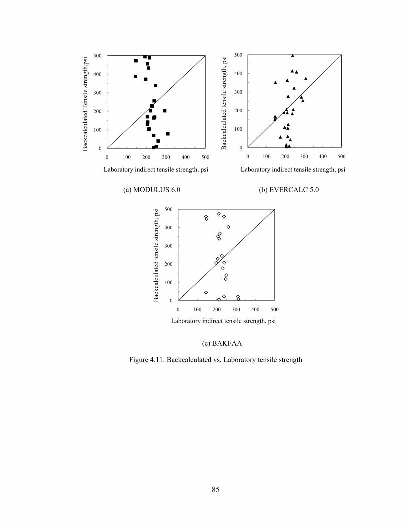
85
(a) MODULUS 6.0 (b) EVERCALC 5.0
(c) BAKFAA
Figure 4.11: Backcalculated vs. Laboratory tensile strength
0
100
200
300
400
500
0 100 200 300 400 500
Bac
kcal
cula
ted
Tens
ile st
reng
th,p
si
Laboratory indirect tensile strength, psi
0
100
200
300
400
500
0 100 200 300 400 500
Bac
kcal
cula
ted
tens
ile st
reng
th, p
si
Laboratory indirect tensile strength, psi
0
100
200
300
400
500
0 100 200 300 400 500
Bac
kcal
cula
ted
tens
ile st
reng
th, p
si
Laboratory indirect tensile strength, psi

86
CHAPTER 5
FINITE ELEMENT MODELING OF FWD DEFLECTION
5.1 Introduction
Finite element modeling (FEM) technique can be used for characterization of the
pavement response under transient load from highway traffic, aircraft gears etc. However,
most of the backcalculation software use layered elastic theory to determine pavement
response, where the applied load is considered static with other assumptions. With the
layered elastic theory, it is not possible to accurately predict pavement response with
different geometric shape, load type, and material properties, especially, if the materials
show elasto-plastic behavior. This study focuses on FEM to predict dynamic response of
pavement due to impulse loading in FWD test. In the FWD test, time-deflection history is
recorded at each and every sensor located at different radial offsets under the short time
dynamic loading. Deflection basin is obtained from the peak displacements of those time-
deflection histories. As such, it is more appropriate to perform dynamic analysis of the
flexible pavement for the accurate prediction of the pavement response. This chapter
covers FEM analysis on different geometries of the layered pavement structure with
varying layer material properties.
5.2 Objectives
The objectives of this study are:
- To model the peak displacements at each sensor due to the impulse generated by a
circular load on the pavement surface. In addition, to determine the time of
87
occurrence of the time-deflection history at each sensor and also, the relative time
lag between the sensors.
- FEM model output is validated by comparing the predicted time-deflection
history to the field measured time-deflection history.
- To determine the variation in the peak deflection with different combination of
the layer moduli.
- The static analysis is also performed by FEM and the output from this analysis is
compared to field FWD basin.
- The static analysis output is compared to that of the dynamic analysis.
- The contours of vertical deflection and von Mises stress are plotted to observe
their distribution over the model.
The time-deflection history data are collected from the FWD test by NMDOT airfield
evaluation team on runway 12-30 in Clayton Airport. The test was done with JILS FWD
20T. Only one data was used due to significant time requires for FEM study. The
information about the layer thicknesses and properties are obtained from the core log of
the runway.
5.3 FEM Model Description
The dynamic response characterization by finite element method needs the development
of a model that can be representative of the field condition. To develop a model of the
multi-layered flexible pavement structure, the following steps were involved:
• Selection of model geometry.
• Assignment of layer property.

88
• Meshing of the model, i.e. discretization of the model geometry with the
appropriate elements.
• Imposing the boundary condition that matches with that during the field test.
• Application of dynamic loading criteria, i.e. determination of the amplitude
pattern for the application of dynamic load during FWD test.
5.3.1 Model Geometry
The geometry of the model in finite element analysis is an important factor to accurately
predict the model behavior under load. From the core log information it is evident that
airport pavements have mainly three different layers and they are surface, base, and
subgrade, respectively. During the FWD test, the load is applied on the pavement surface
through a steel plate with a radius of 6 inches. The short time loading pulse causes an
instantaneous response of the pavement surface. The sensors at the different radial
locations record the vertical movement of the pavement as shown in the Figure 5.1. At a
certain radius, the surface deflection is assumed to be same in all the radial direction.
Thus, it forms a deflection basin/influence zone.
Seven sensors at different offsets measure the vertical deflections during the test. The
radial distances of the sensors from the loading plate in this project are 0, 8, 12, 18, 24,
36, and 60 inches, respectively. The maximum deflection is recorded at the loading point
and gradually, decreases with the increase in the distance. For the finite element
modeling of multi layered pavement structure, different geometries are used by the
researchers for the analysis. These model geometries can be either 2D plane strain, axi-
symmetric or 3D cube.

89
The two-dimensional plane strain model is used by a number of researchers to
characterize the behavior of pavement (van Metzinger and McCullough 1991, and Lytton
et al 1993). It requires little computation time and memory storage for the analysis.
However, it can represent the actual traffic loading and the footprint of the loading is
typically elliptical. It can be used represented by a two semi circles and a rectangle. The
plane strain model only uses the line load (Cho 1997).
The axi-symmetric model is in a geometry developed in 2D and then, revolved around
with reference to a vertical axis to form a cylinder (Thompson 1982, and Nam 1994). The
advantage of this model that it can solve the problem of a 3D structure with the 2D
formulation using cylindrical coordinates. The main limitation of this model is that only
the circular load can be applied on this model. The load assignment from the dual tire is
complicated. Moreover, this model is unable to consider interface shear, though a special
case of all-round radial shear can be analyzed. It can not address the pavement
discontinuities or shoulder conditions. Therefore, this model can be used only for the
region of the pavement far from any cracks or shoulder (Cho 1997).
The 3D FEM can address different issues related to pavement, such as, multiple wheel
loading, nonlinear behavior of base materials, and distresses in pavements (Kuo and
Chou 2004). It can correctly analyze the structural response of pavement-subgrade
systems subjected to static and dynamic loads for new pavements as well as the pavement
with joints, cracks, and discontinuities. The traditional 2D finite element model is not
able to address these problems (Uddin et al 1995). However, it requires long time and
large storage capacity, especially with material the non-linearity (Hjelmstad et al 1997).
Data preparation for this type of model is more labor intensive (Cho et al 1997).

90
This study performs the finite element analysis using both axi-symmetric and quarter
cube geometries of the flexible pavement to represent the actual field condition and
loading configuration of FWD test. The details of the geometries are mentioned below:
Axi-symmetric
Axi-symmetric model is symmetric in all the radial directions with reference to the
vertical axis. Figure 5.2 shows the axi-symmetric structure of the pavement under the
FWD test. It has three layers, i.e. surface, base, and subgrade, of finite thickness
individually. The thicknesses of the surface and base are 2 and 18 inches, respectively.
The influence of the footing becomes insignificant for a homogenous soil if the vertical
distance is considered four to ten times the width of the footing (Yamada 1970, Koswara
1983, and Dunlop et al 1970). The height of the pavement model is assigned 200 inches
and thus, the thickness of the subgrade is limited to 182 inches that is greater than ten
times diameter of the loading plate.
From the field FWD test, it is generally seen that the deflection at the last sensor is too
small and some distances after the last sensor it becomes zero. The reason for this small
deflection at that distance is due to the vertical stress in subgrade and the stress at a large
depth is negligible (Huang 2004). The geometry or the domain size mainly depends upon
the stress distribution in the model. Since most of the deformation takes place in
subgrade, a small domain size is enough to capture the stress and thus, stress is the
important factor for the domain size (Hjelmstad 1997). Considering this fact and to
reduce the computation time, the radial distance of the surface and base courses is limited
to 80 inches. The radial distance of the subgrade is considered 200 inches since the

91
deflection at farther sensor is due to stress in subgrade. A uniform pressure is applied on
an area of 6 inches radius. In FWD test, sensors at different offsets from the loading point
measure the vertical deflection in response to test load. Similar to the FWD test, the
points with the same offsets from the loading point are assigned on the top surface of the
model. The time histories of deflections from the analysis are recorded at these points.
Quarter Cube
The cube of the flexible pavement structure under FWD test has two axes of symmetry.
Therefore, to save the time and storage capacity for the analysis, the quarter of the cube is
modeled in this study for the analysis. The model is shown in the Figure 5.3. Each
individual layer has the finite thickness. Similar to the axi-symmetric model the
thicknesses of the surface and base of this model are 2 and 18 inches, respectively. Both
of the width and height of this model are 200 inches. For this reason, to maintain the
similarity in the dimensions, the length, width and breadth of the quarter cube model are
200, 200, and 200 inches, respectively.
A quarter of the circle with radius of 6 inches is assigned on the top of the pavement for
the application of uniform pressure to match with the FWD test load. To determine the
pavement surface deflections at different sensor locations from the analysis, the points
are assigned along the loading edge (Figure 5.3) according to the offsets of sensors in
field test. The deflections at these points are calculated to observe the nearness of the
analysis values to the field values.

92
5.3.2 Layer Property
The model has three layers: surface, base, and subgrade. The top most layer of the
pavement structure is surface course and it consists of asphalt concrete. The layer
underneath the surface course is base course and it contains the compacted coarse graded
gravelly soil. The bottom layer is the subgrade and it contains the natural soil. Separate
material property has to be assigned for each and every individual layer since they behave
in different manner in response to the impulse during the FWD test. The material
properties are discussed below.
Surface Course
The main constituent of the surface course is asphalt concrete. Asphalt concrete is the
combination of graded aggregate and asphalt binder. Thus, the whole mass has the visco-
elastic property where the aggregate is responsible for elasticity and the binder is for
viscosity. The effect of the visco-elasticity is pronounced at the higher temperature and at
the load with slower rate. The FWD load is instantaneous and thus, the strain is
recoverable. The strain will disappear just after the removal of load (Haddad 1995).
Therefore, the asphalt concrete will behave as elastic material during this very short
duration of loading time. Also FWD test was done at intermediate temperature of the
pavement. For this reason, the surface course is assumed as linear elastic material in this
analysis.
Base Course
In the analysis based on layered elastic theory, the base material is assumed as linear
elastic. To accurately predict the pavement response, material behavior definition should

93
be more realistic. The granular base material can be assumed elastic up to certain limit
and after that it may show plastic behavior. Modeling should consider plastic deformation
beyond the elastic limit. The point at which the plastic deformation begins is known as
yield point (Hibbeler 2005). Once the stress due to the applied load reaches the yield
point, the plastic strain path can be either linear or a curve. In finite element analysis, the
stress-strain distribution has to assigned to address the strain path of a material under
stress variation.
The stress-strain distribution of the granular soil can be determined by performing the
laboratory testing such as triaxial test. In this test, a soil sample is first subjected to an all
around pressure and then, the axial stress is being increased keeping the confining stress
constant (Das 1983). The increased amount of axial stress is known as deviator stress, i.e.
difference between the axial and radial stress (Wood 1990). The application of the
deviator stress continues till the failure of the sample. The region of the stress-strain
distribution before yield point is elastic and the strain is plastic after the yield point.
From the FWD test data and field condition, it is evident that this test is a rapid process.
Therefore, to assign the stress-strain distribution of the base course in finite element
modeling, the load rate in triaxial test should be rapid. The triaxial test is out of the scope
of this study. For this reason, the stress-strain distribution is collected from the study
conducted by Garg nd Thompson (1997). They performed several triaxial tests with
rapid load rate on different types of granular soil. In their study, they first classified the
soils depending on some properties such as unit weight, friction angle. Then, they
performed the triaxial tests on different groups of granular soil. The soil with known
friction angle can be assumed to have the same stress-strain distribution as it observed

94
from the study of Garg and Thompson (1997). For this reason, this study conducted the
direct shear test of the aggregate in base course to measure the shear strength as well as
the angle of friction (ASTM D3080-04) in the laboratory. The particle size distribution
test was also measured to aid in classification of the base material. Generally, the base
material from the airport does have the friction angle of 39 degree (from direct shear test
in the laboratory). According to the Garg and Thompson (1997) the soil is classified as
CL-5 sp. The stress-strain distribution is then obtained from the rapid shear test (triaxial
test with rapid load rate).
The stress-strain distribution of the granular material for the base course is mentioned in
the Figure 5.4. This distribution is assigned in the analysis to integrate the real property
of the base material. For the analysis, the yield point of this stress-strain distribution is
considered 70 psi since the part of the curve before this yield stress can reasonably be
assumed as linear elastic. The base is assumed to show plasticity whenever the stress at
any point in this layer due to FWD load will exceed the deviator stress of 70 psi. The
initial modulus of elasticity for the base material is assumed according to the guideline
from MEPDG (2008).
Subgrade
The subgrade contains the natural soil. Similar to the base material, the stress-strain
distribution of the subgrade can also be determined from triaxial test that can be used as
the material property in the finite element analysis. To perform the triaxial test of the
subgrade soil was out of the scope of this study. As mentioned previously, the FWD load
is instantaneous and the subgrade does not have much time to drain the pore water during
95
the FWD test. The consolidated undrained triaxial test data is assumed as the accurate
stress-strain distribution of the subgrade for the considerations of FWD test. A number of
researchers and organizations have performed triaxial tests on different types of soil. The
subgrade soil in the Clayton airport was found silty clay from the soil index property
determined by laboratory test. Then, for the assignment of the subgrade stress-strain
distribution, the triaxial data are collected from (Slope Stability 2003). Figure 5.5 shows
the stress-strain distribution of the subgrade. As mentioned earlier in the case of base
material, the subgrade will start showing plasticity whenever the stress at any point in this
layer will reach the yield point. The yield stress in this distribution is assumed to be 1.5
T/sft (20.84 psi). And taken into consideration, the stress-strain path in the laboratory
triaxial test is assigned in the analysis to address the material behavior.
The dynamic analysis of the multilayered flexible pavement structure by finite element
method is performed in this study using different combinations of initial layer moduli.
The modulus of elasticity of different individual layers is mentioned in Table 1.
5.3.3 Meshing of Model
Mesh assignment is an important influencing factor in the finite element modeling. The
accuracy of the model is affected by the quality of the mesh. The situation is more
complicated in case of dynamic analysis because the wave travel time depends on the
wave velocity and the length of the mesh. Another critical situation is the meshing near
the loading area as there may be a sharp change in the stress. The mesh assignment for
the models is mentioned below.

96
Axi-symmetric
The axi-symmetric model of the multi layered flexible pavement structure is meshed
finely near the loading region. The region with the sensor points is also finely meshed to
ensure the smooth movement of the stress wave through the medium. The region farther
from the loading region is not as critical as the region near the loading region. Therefore,
the mesh in that region can be coarser to perform the analysis faster. This model is of
irregular geometry, i.e. the length and thickness of the surface and base course are
smaller than those of the subgrade. The surface and base courses are near to the loading
and sensor location whereas the subgrade is farther away from the loading area. The
surface and base are meshed with smaller elements and the subgrade is meshed with
coarse elements. During the meshing with different sized elements with maintaining
regular geometry of the model, the mesh transition is done according to the Figure 5.6.
The analysis is performed in ABAQUS/Explicit. The 4-noded quadrilateral element is
used for the mesh assignment. The aspect ratio of the mesh elements were kept between 1
and 2 all through the model. Aspect ratio is defined as the ratio of the longest dimension
to the shortest dimension (Logan 2007).
Quarter Cube
The quarter cube model of the multilayered pavement structure is meshed with
hexahedral or brick element and the meshing of the model is mentioned in Figure 5.7.
Each individual element has eight nodes. In this analysis, the region near to the loading
area is more critical than that farther away. So, the finer mesh is necessary for the loading
zone whereas the mesh can be coarser near the end. The model developed for this study is

97
cube with identical length, breadth, and height. This geometry leads to the uniform
meshing of the model though it increases the analysis time and needs more storage of the
memory. The coarse mesh in the farther region is avoided due to maintain the aspect ratio
between 1~2. Aspect ratio is an important factor in the analysis and the variation of the
aspect ratio is responsible for the accuracy (Logan 2007).
The parameters of the mesh are summarized for both axi-symmetric and quarter cube in
Table 5.2. It provides the information about the nodes and elements of the model during
mesh assignment.
5.3.4 Boundary Condition
Boundary condition is the known condition of the force and displacement, i.e. known
values of the force and displacements at the nodes. The finite element analysis in
ABAQUS involves two stages for the analysis. The first stage contains the initial phase
of the model whenever there is no load applied on the model. The second stage contains
the analysis phase and in this phase, the pavement response is analyzed with the
application of the load. Therefore, the boundary condition is different in those steps.
Based on the field observation of pavement structure, The assignment of boundary
condition on this model is described below.
Axi-symmetric
There is no load on the pavement surface before and after the application of the FWD test
load. The interfaces at the two adjacent layers are fully bonded (slip is not allowed). The
roller supports are assigned at the vertical left end to allow the vertical movement as well
as restraining the horizontal movement. The qualitative diagram of the boundary

98
condition of the subgrade is mentioned in the Figure 5.2. The length of surface and base
course of this model is assigned 80 inches as mentioned earlier. At the right end of this 80
inches block, there is no support. There may be chance of vertical movement at this end.
For this reason, the vertical movement is not restrained here. The tensile strength in the
soil is negligible. The surface is only of 2 inches that is not enough to develop tensile
force to cause zero deflection. The right end of the bottom block (subgrade) is restrained
to move in the horizontal direction and rollers are assigned as the support. The presence
of the rigid bed rock is assumed at the bottom the subgrade that leads to no deflection at
the interface of the rigid/stiff layer and subgrade. For this reason, the bottom of the model
is assigned with the hinge to restrain the translational movement in all directions.
Quarter Cube
This study performs the finite element analysis with the application of 9 kip test load. To
generate this load, a uniform pressure of 79.6 psi is applied over a quarter of the circle
with the radius of 6 inches. There is no additional load on the pavement surface before
and after the application of the FWD load. The interface of the two adjacent layers is
assumed to be fully bonded, i.e. slip between the two adjacent layers is not allowed. In
response to the FWD load, the deflection becomes zero at some depth and it indicates the
presence of rigid layer at this point. To address this phenomenon, the hinge supports are
assigned at the bottom of the model and thus, constrains the bottom from moving along
both vertical and horizontal directions. The two intersected edges with the loading point
(along two axes of symmetry) are free to move in vertical direction and are restrained in
the horizontal direction from adjacent material. In this model, these edges are assigned
with the roller supports to ensure this behavior of the structure. There is no movement in

99
horizontal direction some distances after the last sensor location. For this reason, the
roller supports are also assigned at the ends of the model. The boundary condition of the
model is more clearly described in Figure 5.3.
5.3.5 Loading Criteria
This study performs both static and dynamic analyses of the airport pavement to evaluate
FWD deflection basins. The load applications in these two different types of analyses are
described below.
Static Load
The FWD load is the function of time. In the static analysis, the load is constant with time
variation. For this reason, only the peak of the load-time history is used as a static load in
this study. The magnitude of the peak is 9 kips and it develops a pressure of 79.6 psi on
the loading plate of 6 inches radius.
Dynamic Load
The purpose of this analysis is to determine the dynamic response of the pavement under
FWD test. To accurately predict the pavement response, it is necessary to follow the
actual amplitude pattern to apply the impulse. For this reason, the time-load history is
collected from the Clayton Airport. This model is analyzed with the application of
impulse with the magnitude of 9 kip. The time dependent loading pattern is assigned
according to the field test. A pressure of 79.6 psi is applied on the loading area and then,
this pressure is integrated with the field time-amplitude variation to match with the load-
time history under field test. The time-load history is shown in the Figure 5.8. It is

100
observed from the figure that the duration of the load is 25 milliseconds and the peak has
attained at 10 milliseconds. The response of the multilayered flexible pavement structure
(time-deflection histories of the sensors) is mentioned in Figure 5.9.
5.4 Finite Element Analysis
The finite element analysis is performed in ABAQUS after the development of the
model. Both static and dynamic conditions of the FWD test are considered in the
analyses. Two different geometries axi-symmetric and quarter cube are used separately
for the static and dynamic analysis. The model is analyzed for a number of layer moduli
combinations as mentioned in the MEPDG according to the layer properties. The main
purpose of this analysis is to determine the FWD deflection basin. The time deflection
history at the specified sensor locations are recorded from the dynamic analysis.
Analyzed time-deflection histories are then compared to the field time-deflection
collected from FWD test. The deflection basin obtained from the field test was also
compared with the analyzed peak deflections at the sensor points.
5.4.1 Static Analysis
Axi-symmetric
The finite element analysis of the axi-symmetric model is performed with the application
of static load. The deflections of the points at different radial offset are determined to get
the FWD deflection basin. The deflection basins of this model are shown in Figure
5.10(a) to (f) for different combinations of layer modulus. For the detailed discussion, the
vertical deflection is determined at the layer interface. The contour of vertical deflection
and von Mises stress is also plotted to observe the distribution although the model.
101
Quarter Cube
The static analysis is performed on the quarter cube model to observe the 3D static
response of the pavement under FWD test. Similar to the axi-symmetric model, the
vertical deflections are determined at different distances to evaluate the FWD deflection
basins. The deflection basins for different combinations of layer modulus are shown in
Figure 5.11(a) to (f). From this analysis, the vertical deflection is also determined at the
layer interface. To observe the distribution of the deflection and stress over the model, the
contours of vertical deflection and von Mises stress are plotted.
5.4.2 Dynamic Analysis
Axi-symmetric
The deflection basins developed from the analysis are shown in the Figure 5.12(a) to (f).
The deflections of the sensor are calculated at each sensor point and then compared to the
field values. The field values are collected from the FWD peak deflection at the runway
12-30 in Clayton Airport. The analyses are carried out for different layer moduli
combinations to match the calculated deflections with the field values. In each and every
plot, the modulus combinations are mentioned in the layer diagram. The layer moduli
combinations are mentioned in the Table 5.1. The time-deflection histories are also
determined at the sensor locations. From these results, the peak deflections and their time
of occurrence, the time lag between the loading time and the response at the sensor as
well as between the two successive sensors are recorded. These were done to check the
nearness of the analysis results to the field values. The time-deflection histories from the
pre defined sensor points are mentioned in the Figure 5.13(a) to (f).
102
Quarter Cube
The time deflection history of the points located at different distances is analyzed for
different combinations of layer moduli. During the analysis, the property of each
individual layer was assigned according to the material type mentioned earlier. The
duration of the analysis was 100 milliseconds and this time duration was set up due to
observe the variation of the deflection with time. The peak deflection was then extracted
from each analyzed time-deflection history of the specific points. These peak deflections
at different offsets thus form a deflection basin. The deflection basins as well as the time-
deflection histories for different combinations of layer moduli are then compared to the
field FWD values. The layer moduli combinations for which the analyses were performed
are mentioned in the Table 5.1. The time of peak deflection occurrence at each point is
one of the major concerns in this study. This time is then compared to the original time of
occurrence to observe the difference. The time lag between the peak deflections at two
successive sensors is also investigated. As mentioned earlier, the field FWD time –
deflection history is collected from the test performed in Clayton. These data are used in
this study to validate the analysis results from the model.
5.5 Discussion
5.5.1 Static Deflection Basin
Axi-symmetric
Figure 5.10(a) to (f) shows the FWD deflection basins for the combinations of layer
modulus as mentioned in Table 5.1. The deflection basin plotted for each layer modulus
103
combination is compared to the deflection basin from the runway 12-30 in Clayton
airport.
Figure 5.10(a) to (c) shows the deflection basin for surface and base modulus of 200 and
40 ksi, respectively, whereas the subgrade modulus is 24, 17, and 8 ksi. The peak
deflection is 20.88 mils as shown in Figure 5.10(a) and the deflection diminishes as the
distance increases. The deflection at the last sensor is 0.56 mils. The peak deflection from
the field deflection basin is 35 mils and the deflection at the last sensor is 2.25 mils. The
difference between the field and analyzed at the first sensor is 14.22 mils.
Figure 5.10(b) shows the deflection basin for the surface, base, and subgrade modulus of
200, 40, and 17 ksi. The deflection at the first sensor is 22.85 mils and the difference with
the field deflection is 12.15 mils. The deflection at the last sensor is 0.84 mils whereas
that in the field is 2.25 mils. Figure 5.10(c) shows the deflection basin for the layer
modulus combination of 200, 40, and 8 ksi. It is observed that the deflection at the first
sensor is 28.86 mils with the difference of 6.14 mils from the field deflection. The
deflection at the last sensor is 2.03 mils that is closest to 2.25 mils from field data.
The surface modulus is raised to 300 ksi for the next three analyses while the base and
subgrade modulus kept constant as earlier. Figure 5.10(d) shows the deflection basin for
modulus combination of 300, 40, and 24 ksi. The deflection at the first sensor is 20.57
mils and the difference from the field is 14.43 mils. The deflection at the last sensor is
0.57 mils and that in the field is 2.25 mils.
Figure 5.10(e) shows the deflection basin for the modulus combination of 300, 40, and 17
ksi. The peak deflection is 22.499 mils and the difference is 12.501 mils. The deflection

104
at the last sensor is 0.85 mils. Figure 5.10(f) shows the deflection basin for modulus
combination of 300, 40, and 8 ksi. The peak of the deflection basin is 28.33 mils with the
difference of 6.67 mils from the field. The deflection at the lat sensor is 2.06 mils which
is close to the field value (2.25 mils).
Quarter Cube
Figure 5.11(a) to (f) shows the FWD deflection basins for the quarter cube model. The
combinations of layer modulus as mentioned in Table 5.1. The deflection basin plotted
for each layer modulus combination is compared to the deflection basin from the runway
12-30 in Clayton airport.
Figure 5.11(a) to (c) shows the deflection basin for surface and base modulus of 200 and
40 ksi, respectively, whereas the subgrade modulus is 24, 17, and 8 ksi. The peak
deflection is 17.37 mils as shown in Figure 5.11(a) and the deflection diminishes as the
distance increases. The deflection at the last sensor is 0.48 mils. The peak deflection from
the field deflection basin is 35 mils and the deflection at the last sensor is 2.25 mils. The
difference between the field and analyzed at the first sensor is 17.63 mils.
Figure 5.11(b) shows the deflection basin for the surface, base, and subgrade modulus of
200, 40, and 17 ksi. The deflection at the first sensor is 16.18 mils and the difference with
the field deflection is 18.82 mils. The deflection at the last sensor is 0.32 mils whereas
that in the field is 2.25 mils. Figure 5.11(c) shows the deflection basin for the layer
modulus combination of 200, 40, and 8 ksi. It is observed that the deflection at the first
sensor is 20.75 mils with the difference of 14.25 mils from the field deflection. The
deflection at the last sensor is 1.13 mils that is just half of 2.25 mils from field data.

105
The surface modulus is raised to 300 ksi for the next three analyses while the base and
subgrade modulus kept constant as earlier. Figure 5.11(d) shows the deflection basin for
modulus combination of 300, 40, and 24 ksi. The deflection at the first sensor is 15.41
mils and the difference from the field is 19.59 mils. The deflection at the last sensor is
0.32 mils and that in the field is 2.25 mils.
Figure 5.11(e) shows the deflection basin for the modulus combination of 300, 40, and 17
ksi. The peak deflection is 16.56 mils and the difference is 18.44 mils. The deflection at
the last sensor is 0.48 mils. Figure 5.11(f) shows the deflection basin for modulus
combination of 300, 40, and 8 ksi. The peak of the deflection basin is 19.84 mils with the
difference of 15.16 mils from the field. The deflection at the lat sensor is 1.14 mils and
the difference with the field value is 1.11 mils.
5.5.2 Dynamic Deflection Basin and Time History
Axi-symmetric
Figure 5.12(a) to (f) shows the deflection basins determined by the dynamic analysis with
the finite element method. These figures show the deflections of the same model with
same stress-strain distribution but with different combinations of initial modulus of
elasticity at each layer.
In Figure 5.12(a) to (c), the surface and the base moduli are 200 and 40 ksi, respectively.
The subgrade modulus is varied and they are 24, 17, and 8 ksi. And from the analysis, it
is found that the peak deflection is equal or near to 15 mils. The maximum deflection is
recorded at the center point and there is a sharp drop in the deflection. From, 10 to 20
inches the decreasing rate of deflection is too low. It may due to the application of
106
plasticity in the stress-strain distribution in the base layer. The thickness of the surface
course is 2 inches and the base is just underneath the surface. Therefore, the stress
developed in the base course due to the FWD load will be of significant amount and there
is a possibility of this stress to cause nonlinear strain (may show the plastic strain). The
deflections get zero at 36 inches from the center point, i.e. fifth sensor. From the figures it
is also evident that the peak deflection of the basin from the field is 35 mils and there is a
sharp drop in the deflection values. The decreasing rate of the deflection value is getting
lower at the farther sensor points and the minimum deflection is 2 mils at the outermost
sensor. The deflection basins for the mentioned layer moduli combinations from the
Figure 5.12(a) to (c), do not match with the field values.
The analyses were repeated for the modified layer moduli combinations with surface
modulus of 300 ksi. Here, also the values of subgrade modulus are 24, 17, and 8 ksi while
the surface and base modulus are kept constant at the values of 300 and 40 ksi,
respectively. Figure 5.12(d) to (f) show the deflection basins analyzed for these new
combinations. The duration of the analyses was increased to 100 milliseconds. There is a
possibility of the stress wave with low velocity that may increase the travel time and with
the analysis duration of 60 milliseconds the deflection at some sensors may be zero due
to the delay in wave propagation. For this reason, the duration of the analysis is increased
to capture the waves at the sensors. From the Figures 5.12(d) to (f), it is observed that
there is no significant influence of the surface modulus variation on the deflection. The
increase in analysis time, determined the non zero deflections at the farther sensors. In the
previous analyses as mentioned in the Figure 5.12(a) to (c), the deflection is zero at the
fifth sensor. Due to the increase in analysis time, the stress wave has more travel time

107
than that of the previous analyses to reach the farthest sensor and thus, the non zero
deflection is recorded at that point.
The time-deflection histories of the sensors at different radial offsets are determined to
perform the tasks as mentioned in the objectives. The Figures 5.13(a) to (f) show the
time-deflection histories for different combinations of layer moduli. The first three
analyses were performed with the duration of 60 milli seconds. In these combinations the
subgrade modulus were 24, 17, and 8 ksi while keeping the surface and base modulus
constant at the values of 200 and 40 ksi, respectively.
From the Figure 5.13(a), it is seen that the peak deflection at the first sensor occurs at
22.5 milli seconds and those of the second, third, fourth and fifth sensor occur at 33.6,
43.2, 56.7, and 60 milli seconds. The sixth and seventh sensors show the zero deflection.
Here, in the analyses, it is observed that there is a significant amount of time lag of the
peak deflection occurrence between the sensors. In the field test, the responses of the
sensors were instantaneous and simultaneous. The analysis results give the indication of
the larger travel time, i.e. low velocity, of the stress wave through the model. The other
observation is that the deflections at the sixth and seventh sensors are recorded zero. The
same incidents are observed in the Figures 5.13(b) and (c).
In Figure 5.13(b), the peak deflections are recorded 22.2, 33, 44.1, 59.4, and 60 milli
seconds at the first, second, third, fourth, and fifth sensor, respectively. Here, the sixth
and seventh sensor points also determine the peak deflection of zero. The time of
occurrence of peak deflections are recorded 22.5, 33.6, 45.3, and 60 milli seconds at first,
second, third, and fourth sensor as shown in the Figure 5.13(c). Still, some sensors farther

108
from the loading point show the zero vertical deflection that is undesirable. This incident
may be due to the large propagation time of wave through the model. For this reason, the
analysis time is increased to 100 milli seconds for the next three analyses. The surface
modulus is increased to 300 ksi while keeping the base modulus at 40 ksi. The subgrade
modulus variation is the same as followed in the previous analyses.
Figures 5.13(d) to (f) show the time-deflection histories for the new combinations of
layer moduli and analysis duration. There is no significant change in the peak deflection
at the first sensor as it was determined before. In the previous analyses, it was observed
that the peak deflection at the fifth and the farther sensor is zero. Due to the increase in
the analysis time, the time-deflection histories at the farther sensors are recorded for
larger time duration. As a result, the fifth and sixth sensors have extracted the larger peak
deflections. The time-deflection histories for surface, base, and subgrade modulus of 300,
40, and 24 ksi, respectively, are plotted in Figure 5.13(d). The time of occurrence of the
peak deflections at the seven sensors are 22, 31.5, 44.5, 62.5, 79.5, and 100 milli seconds.
The peak deflections at the last two sensors are determined at the same time, i.e. 100 milli
seconds. The time lag between the successive sensors is still large but in the field FWD
test, it was simultaneous. In Figures 5.13(e) and (f), the non-zero vertical deflections are
recorded at the fifth sensor and so on. The time lags in these analyses are still large.
Quarter Cube
The dynamic analysis in finite element method was performed for the aforementioned
layer moduli combinations though the stress-strain distribution for each individual layer
109
is still same. The deflection basins obtained from the 3D dynamic analysis are mentioned
in Figure 5.14(a) through (f).
In Figures 5.14(a) to (c), the deflection basins are mentioned for the surface and base
modulus of 200, and 40 ksi, respectively, while changing the subgrade modulus 24, 17,
and 8 ksi, respectively. The peak deflection at the first sensor is about 10 mils in Figure
5.14(a) and it gradually decreases to zero at the last sensor. The peak deflection is 35 mils
in Clayton FWD deflection basin and it is three times higher than analyzed peak
deflection. The subgrade modulus is 17 ksi in Figure 5.14(b) and the peak deflection is
less than 10 mils that give the indication that the change in subgrade modulus does not
have the pronounced effect on the peak deflection value. The deflection basin for this
modulus combination does not also match with field values. The subgrade modulus is 8
ksi in Figure 5.14(c) and the peak deflection is 10 mils. The deflection reached zero
magnitude at the sixth sensor (distance: 36 inches). However, the deflection basin for this
combination of layer moduli does not match with field values.
To observe the farther effect of modulus variation on the analysis results, the surface
modulus was assigned 300 ksi while keeping the base and subgrade modulus same as
before. Figure 5.14(d) to (f) shows the deflection basin with surface and base modulus of
300 and 40 ksi, respectively, whereas the subgrade modulus is 24, 17, and 8 ksi,
respectively. The peak deflection is about 10 mils in Figure 5.14(a) that is much smaller
than the field value. The deflection at the seventh sensor (distance: 60 inches) is zero but
in the field FWD data, the deflection is non zero. So, change in surface modulus does not
have significant effect in the analysis of this model. In Figure 5.14(e) and (f), the surface
and base modulus are the same whereas the subgrade modulus is 17 and 8 ksi. And

110
variation in the subgrade modulus does not affect the deflections. This model with the
mentioned combinations of layer moduli is very stiff since the deflections at the points
are much smaller than the field deflections.
The time-deflection histories at different sensor points are analyzed and mentioned in the
Figure 5.15(a) through (f). The time-deflection history in Figure 5.15(a) is analyzed for
the surface, base, and subgrade modulus of 200, 40, and 24 ksi, respectively. The peak
deflection at the first sensor point occurs at 20 milli second and it is 9.87 mils. The peak
value at the second sensor is observed 3.82 mils at 30 milli second and the time lag is
about 10 milli second. The peak values of the time-deflection histories at the third, fourth,
fifth, and sixth sensor are 2.29, 1.68, 1.26, and 0.64 mils, respectively. The peak at the
last sensor is 0.066 mils. It is clearly evident from the Figure 5.15(a) that the time lag
between the peak deflection values at the two adjacent sensors are significantly large
whereas the peak deflections from the field FWD data are with negligible time lag as
mentioned in Figure 5.9.
Figure 5.15(b) shows the time-deflection histories for the modulus combination of 200,
40, and 17 ksi, respectively. The peak deflection of the first sensor is 8.26 mils and it has
attained at 20 milli second. After some time lagging, the peak of the second sensor (3.58
mils) has attained at 25 milli second and the time lag of 5 milli second is a significant
amount whereas the time lag in field data is nearly negligible. The peak deflections of the
time-deflection histories at third, fourth, fifth, and sixth are 2.19, 1.9, 1.36, and 0.51 mils,
respectively, and they show the time lag larger than that in field FWD data. The peak
(0.057 mils) at the last sensor has occurred at 94 milli second and it shows greater time
lag than the field test.

111
The time-deflection histories of the sensors for the surface, base, and subgrade modulus
of 200, 40, and 8 ksi, respectively, are mentioned in Figure 5.15(c). At 19 milli second,
the peak deflection of the first sensor is 9.84 mils. And at 32 milli second, the peak is
found 3.78 mils at the second sensor point. So, the time lag is 13 milli second and it is
very high. The peak deflections of the third, fourth, fifth, and sixth sensors are 2.24, 1.62,
1.18, and 0.46 mils, respectively. These peak values occur at 47, 60, 71, and 100 milli
second. The deflection at the last sensor is almost zero. The figure shows the response is
not instantaneous and the times lag between the peak deflections of the adjacent sensors
are larger than that from the field value.
In the next three analyses, the surface modulus was increased to 300 ksi while keeping
the base and subgrade moduli same as before. Figure 5.15(d) to (f) shows the time-
deflection histories for surface and base modulus of 300, and 40 ksi, respectively. And
the subgrade moduli are 40, 24, and 17 ksi. In Figure 5.15(d), the peak deflection at the
first sensor is found 9.46 mils at 19 milli second and that at the second sensor is found
3.83 mils at 31 milli second. The time lag is 12 milli second between the first and second
sensor. The peak deflections of the time-deflection histories at the third, fourth, fifth, and
sixth sensors are 2.27, 1.47, 1.198, and 0.65 mils, respectively. And the time of
occurrence of these peak values are 43, 60, 71, and 100 milli second, respectively. Still,
the time lag is so high.
The time-deflection histories for the moduli combination of 300, 40, and 17 ksi are
plotted in Figure 5.15(e). The peak deflection of the time history in the first sensor is
found 9.47 mils at 20 milli second and in the second sensor, it is found 3.82 mils at 31
milli second. The resulting time lag is 11 milli second. The peak deflections of the time-
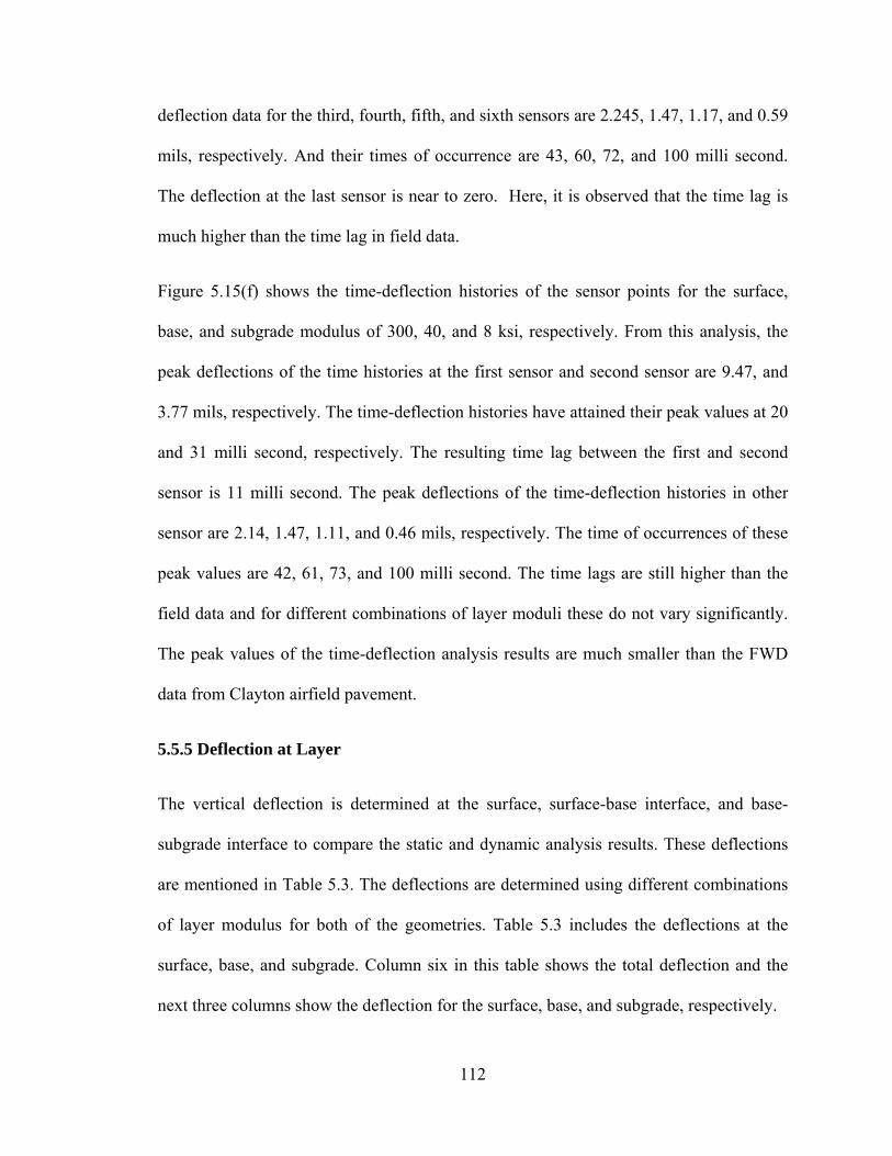
112
deflection data for the third, fourth, fifth, and sixth sensors are 2.245, 1.47, 1.17, and 0.59
mils, respectively. And their times of occurrence are 43, 60, 72, and 100 milli second.
The deflection at the last sensor is near to zero. Here, it is observed that the time lag is
much higher than the time lag in field data.
Figure 5.15(f) shows the time-deflection histories of the sensor points for the surface,
base, and subgrade modulus of 300, 40, and 8 ksi, respectively. From this analysis, the
peak deflections of the time histories at the first sensor and second sensor are 9.47, and
3.77 mils, respectively. The time-deflection histories have attained their peak values at 20
and 31 milli second, respectively. The resulting time lag between the first and second
sensor is 11 milli second. The peak deflections of the time-deflection histories in other
sensor are 2.14, 1.47, 1.11, and 0.46 mils, respectively. The time of occurrences of these
peak values are 42, 61, 73, and 100 milli second. The time lags are still higher than the
field data and for different combinations of layer moduli these do not vary significantly.
The peak values of the time-deflection analysis results are much smaller than the FWD
data from Clayton airfield pavement.
5.5.5 Deflection at Layer
The vertical deflection is determined at the surface, surface-base interface, and base-
subgrade interface to compare the static and dynamic analysis results. These deflections
are mentioned in Table 5.3. The deflections are determined using different combinations
of layer modulus for both of the geometries. Table 5.3 includes the deflections at the
surface, base, and subgrade. Column six in this table shows the total deflection and the
next three columns show the deflection for the surface, base, and subgrade, respectively.

113
It is observed that for every layer modulus combination, the static deflection is greater
than the dynamic deflection for both of the models. Effect of change of modulus is more
pronounced in static analysis than that in dynamic analysis. From Table 5.3, it is evident
that the decrease in layer modulus causes the increase in the vertical deflection whereas
the dynamic analysis is not affected significantly with the modulus variation.
5.5.4 Contour of Vertical Deflection
Axi-symmetric
The contours are plotted for both static and dynamic analyses cases to observe the
distribution of the vertical deflection over axi-symmetric model. Two different modulus
combinations are selected for these contour plots. The first combination is 200, 40, and 8
ksi and the second combination is 300, 40, and 24 ksi as the surface, base, and subgrade
modulus, respectively.
Figure 5.16 shows the contours of vertical deflection on axi-symmetric model for both
static and dynamic analysis. Figure 5.16(a) shows the contour of static analysis whereas
Figure 5.16(b) is based on dynamic analysis. These contours are plotted for the modulus
combination of 200, 40, and 8 ksi. The legend at the left represents the deflection values
depending upon the color variation. The blue color in the legend shows the maximum
vertical downward deflection whereas the red shows the upward deflection. The color
variation from blue to red represents the vertical downward deflection decreases and
approaches to the upward vertical deflection. From the contour plots of two different
cases, it is observed that the maximum deflection is at the corner of the model where the

114
load is applied. The maximum deflection for static analysis is greater than the dynamic
deflection.
The contours of vertical deflection are again plotted for the modulus combination of 300,
40, and 24 ksi. Figure 5.17 shows the contour plots for this modulus combination. In both
of the cases the peak is observed at the corner as before. From these plots, the maximum
deflection is observed in the same corner region of the model. From the contour plots, it
is observed that the deflections from static analysis are greater than that from dynamic
analysis. For the dynamic analysis, the deflection is higher and concentrated near to the
loading point. In dynamic analysis, the peaks at different sensors were recorded at
different times due to the wave stress propagation through the model. For this reason, the
peak values at the sensors, except the first sensor, are not visible in this contour. On the
other hand, the static analysis shows the peak deflections at every sensor in the same
contour since the load in static analysis is constant with the time variation and the
pavement response to the load is simultaneous.
The contours of the vertical deflection for the other modulus combinations are shown in
the Appendix.
Quarter Cube
Figure 5.18 shows the contours of vertical deflection for quarter cube considering both
static and dynamic analyses cases. The modulus combination of 200, 40, and 8 ksi is
considered for these contour plots. The maximum deflection is observed at the corner of
the model. And the static deflection is greater than the dynamic deflection. And due to

115
time lag, the points other than the top corner of the model do not show the peak
deflection at the same time during dynamic analysis.
Figure 5.19 shows the contours for the modulus combination of 300, 40, and 24 ksi. The
static deflection is also greater than the dynamic deflection. For static analysis, the
contour shows the maximum deflection at every sensor points since the pavement
response has been taken place simultaneously. The contour from dynamic analysis shows
the peak deflections concentrated at the corner and the deflections at other points are very
small due to the time lag.
5.5.5 Contour of Stress
Axi-symmetric
To observe the stress distribution over the axi-symmetric model, the contours are plotted
based on von Mises stress. Both of the static and dynamic analyses are considered for the
contour plots. Figure 5.20(a) shows the contours of von Mises stress for static analsysis
and Figure 5.20(b) shows that for dynamic analysis. The modulus combination of 200,
40, and 8 ksi is considered for this analysis. The legend on the left shows that the red
represents the maximum stress and the blue represents the minimum stress. The color
variation from red to blue indicates the stress variation in descending order. The
maximum stress for static analysis is 51.05 psi and that of the dynamic analysis is 58.61
psi.
Figure 5.21 shows the contours of von Mises stress for 300, 40, and 24 ksi. From the
contours, the maximum of von Mises stress is determined 52.33 psi for static analysis and
63.93 for dynamic analysis.

116
Quarter Cube
Figure 5.22 shows the contours of von Mises stress for quarter cube model. These
contours are plotted for both static and dynamic analysis. The modulus combination of
200, 40, and 8 ksi is assumed for the analysis. The maximum for the static analysis is
observed 41.33 psi and that for the dynamic analysis is observed 45.42 psi.
Figure 5.23 shows the contours for the modulus combination of 300, 40, and 24 ksi. The
maximum stress is observed 44.3 psi for static analysis and that for the dynamic analysiss
is observed 44.5 psi.
5.6 Comparing Static vs. Dynamic Analysis
Figure 5.24 shows the comparison of the static and dynamic analysis for axi-symmetric
model. For the static analysis, six different combinations of layer modulus are considered
as mentioned earlier. The static and dynamic analyses are compared based on the FWD
deflection basin. The nearness of both static and dynamic deflection is also compared to
the field FWD deflection from runway 12-30 in Clayton airport. For axi-symmetric
model, it is observed that the static deflection is greater than the dynamic deflection and it
is closer to the field deflection. Therefore, the static analysis gives better results than the
dynamic analysis for ax-symmetric model.
Figure 5.25 shows the comparison of the static and dynamic analysis for quarter cube
model. The static analysis gives greater deflection than dynamic analysis and it is closer
to the field deflection. It is evident that the static analysis results are better than dynamic
analysis for the prediction of field FWD deflection basin.

117
5.7 Conclusions
The above discussions lead to the following conclusions:
For the same combination of layer moduli, the axi-symmetric and quarter cube
geometries yield different analysis results. The axi-symmetric model shows
higher deflections than that from quarter cube model. The peak deflections from
the axi-symmetric model are closer to the field FWD data for the mentioned
moduli combinations.
From the field FWD data, it is observed that the response of the flexible pavement
under the impulse is instantaneous and the time lags between the successive
sensors are very small. In this study, the analyses show the significant amount of
time lag between the two successive points and also the time of occurrence of the
higher than that of the field data in both of the two different geometries.
For the variation of the combinations of the layer moduli, the surface modulus is
varied from 200 to 300 ksi and the subgrade modulus is varied from 17 to 40 ksi.
The base modulus is kept constant. The analysis results have shown that these
combinations does not affect significantly.
For the mentioned moduli combinations, the peak deflections have not match with
the field values. The moduli combination with lower surface and base modulus
may give the deflection closer to the field data.
The analysis results from the static analysis are closer to the field FWD test data.
The deflection from this analysis is greater than the dynamic analysis.
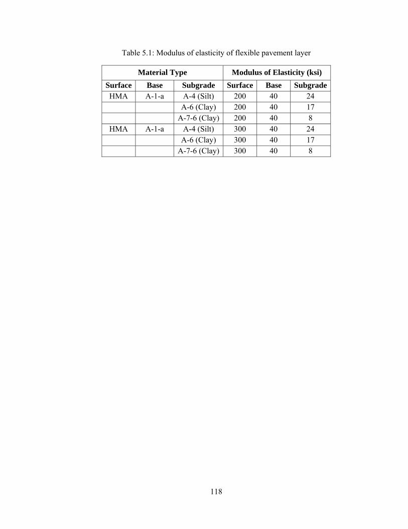
118
Table 5.1: Modulus of elasticity of flexible pavement layer
Material Type Modulus of Elasticity (ksi) Surface Base Subgrade Surface Base Subgrade HMA A-1-a A-4 (Silt) 200 40 24
A-6 (Clay) 200 40 17 A-7-6 (Clay) 200 40 8
HMA A-1-a A-4 (Silt) 300 40 24 A-6 (Clay) 300 40 17 A-7-6 (Clay) 300 40 8

119
Table 5.2: Parameters of the finite element model
FEM parameter Axi-symmetric Quarter cube
Number of nodes 4,440 46,274
Element type CAX4R C3D8R
Number of elements 4,561 49,595

120
Table 5.3: Vertical deflection at the layer interface
Geometry Modulus of Elasticity (ksi)
Type Deflection (mils)
Surface Base Subgrade Total δ1 δ2 δ3
Axi-symmtric
200 40 8 Static 22.8 1 12.32 9.48
Dynamic 15.44 1.32 13.23 0.89
200 40 17 Static 20.8 1 12.39 7.41
Dynamic 15.63 1.34 13.4 0.89
200 40 24 Static 17.4 1.1 9.9 6.4
Dynamic 15.5 1.33 13.28 0.89
300 40 8 Static 28.3 0.6 12.5 15.2
Dynamic 15.47 1.33 13.26 0.88
300 40 17 Static 22.5 0.7 12.49 9.31
Dynamic 15.52 1.33 13.31 0.88
300 40 24 Static 20.6 0.7 12.59 7.31
Dynamic 15.62 1.32 13.42 0.88
Quarter cube
200 40 8 Static 20.8 1.1 9.73 9.97
Dynamic 11.55 1 10.05 0.5
200 40 17 Static 17.4 1.15 9.86 6.39
Dynamic 11.6 0.98 10.13 0.49
200 40 24 Static 16.2 1.1 10 5.1
Dynamic 11.7 0.96 10.25 0.49
300 40 8 Static 19.8 0.7 9.3 9.8
Dynamic 10.89 0.95 9.5 0.44
300 40 17 Static 16.6 0.8 9.49 6.31
Dynamic 11.1 0.95 9.71 0.44
300 40 24 Static 15.4 0.7 9.6 5.1
Dynamic 11.27 0.98 9.85 0.44

121
Figure 5.1: The zone of influence during FWD test
LoadInfluence zone
Subgrade
Base
Surface
Geophones

122
Figure 5.2: Qualitative diagram of the Axi-symmetric model of flexible pavement
Surface: h1, E1, υ1, ρ1
Base: h2, E2, υ2, ρ2
Subgrade: h3, E3, υ3, ρ3
R
Z
Hinge Supports
Rol
ler S
uppo
rts
Rol
ler S
uppo
rts
Sensor indicator
Load

123
(a)
(b)
Figure 5.3: Qualitative diagram of the Quarter cube model of flexible pavement
Y
Z
Y
X
Surface
Base
Subgrade Subgrade
Base
Surface
Y
Z
X
FWD test load over the one quarter of the circular loading area
Sensor indicator

124
Figure 5.4: Stress-strain distribution of the granular soil in base course (Garg and Thompson,
1997)
0
10
20
30
40
50
60
70
80
90
100
0 3 6 9 12
Dev
iato
r stre
ss (p
si)
Axial strain (%)

125
Figure 5.5: Stress-strain distribution of subgrade soil from triaxial test (Slope stability 2003)
0
0.5
1
1.5
2
2.5
0 4 8 12 16 20
Dev
iato
r stre
ss (T
/sft)
Axial strain (%)

126
Figure 5.6: Mesh refinement of the axi-symmetric model

127
Figure 5.7: Mesh refinement of the quarter cube model

128
Figure 5.8: Amplitude pattern of the impulse in the FWD test
0
2
4
6
8
10
0 5 10 15 20 25
Load
(kip
s)
Time (milliseconds)
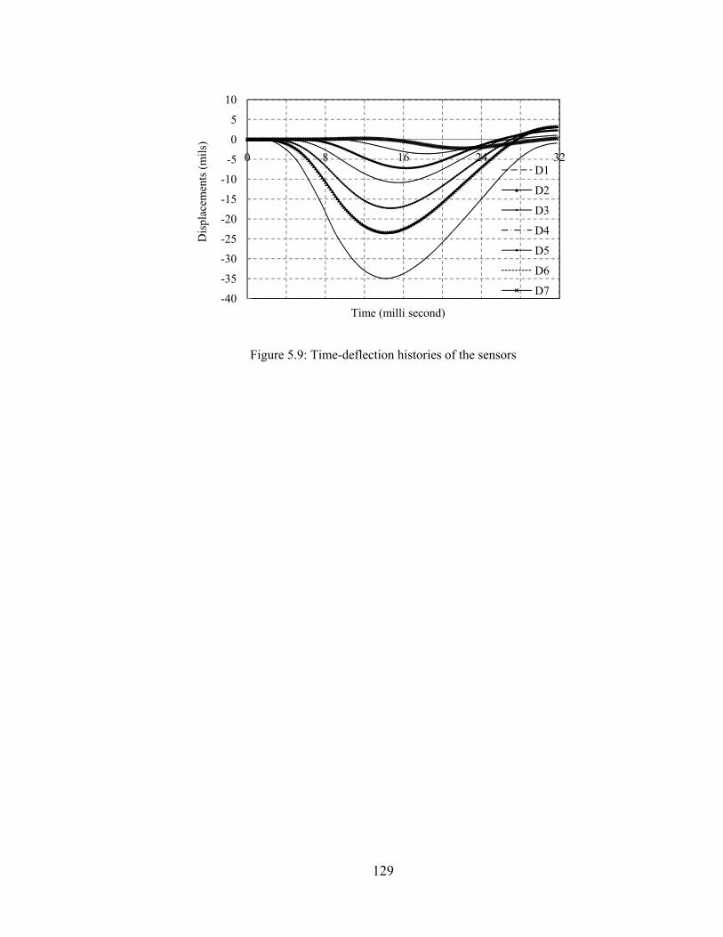
129
Figure 5.9: Time-deflection histories of the sensors
-40
-35
-30
-25
-20
-15
-10
-5
0
5
10
0 8 16 24 32
Dis
plac
emen
ts (m
ils)
Time (milli second)
D1
D2
D3
D4
D5
D6
D7

FFigure 5.10: DDeflection ba
-40-35-30-25-20-15-10
-50
Dis
plac
emen
t (m
ils)
-40-35-30-25-20-15-10
-50
Dis
plac
emen
t (m
ils)
-40-35-30-25-20-15-10-50
Dis
plac
emen
t (m
ils)
asins analyzed
050505050
0
0
050505050
0
130
(a)
(b)
(c)
d for different
static analys
20Sensor off
20Sensor offs
20Sensor offs
t layer moduli
sis)
40fse t (inches)
FEA
Clayt
40se t (inches)
FEAClayton
40se t (inches)
FEA
Clay
i combination
60
ton
60
n
60
A
yton
ns (axi-symmmetric

FFigure 5.10: DDeflection ba
-40-35-30-25-20-15-10
-50
Dis
plac
emen
t (m
ils)
-40-35-30-25-20-15-10-50
Dis
plac
emen
t (m
ils)
-40-35-30-25-20-15-10-50
Dis
plac
emen
t (m
ils)
asins analyzed
050505050
0
0
050505050
0
131
(d)
(e)
(f)
d for different
static analys
20Sensor offs
20Sensor offs
20Sensor offs
t layer moduli
sis)
40se t (inches)
FEAClay
40se t (inches)
FEAClayt
40se t (inches)
FEAClay
i combination
60
Ayton
60
ton
60
ton
ns (axi-symmmetric

Figure 5.11: Deflection b
-40-35-30-25-20-15-10-50
Dis
plac
emen
t (m
ils)
-40-35-30-25-20-15-10
-50
Dis
plac
emen
t (m
ils)
-40-35-30-25-20-15-10
-50
Dis
plac
emen
t (m
ils)
asins analyze
050505050
0
050505050
0
050505050
0
132
(a)
(b)
(c)
ed for differen
static analys
20Sensor offse
20Sensor offs
20Sensor off
nt layer modu
sis)
40e t (inches)
FEAClayto
40se t (inches)
FEAclayto
40fse t (inches)
FEAClayto
uli combinatio
60
on
60
n
60
on
ons (quarter cube
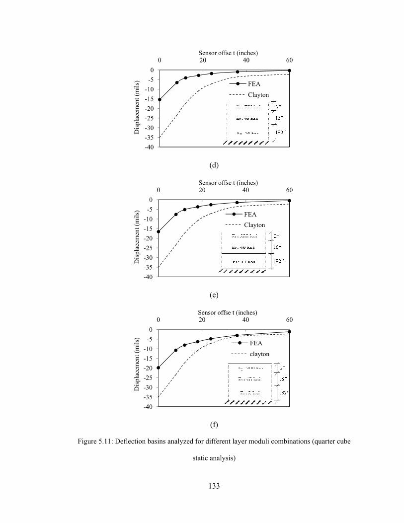
Figure 5.11: Deflection b
-40-35-30-25-20-15-10
-50
Dis
plac
emen
t (m
ils)
-40-35-30-25-20-15-10
-50
Dis
plac
emen
t (m
ils)
-40-35-30-25-20-15-10
-50
Dis
plac
emen
t (m
ils)
asins analyze
050505050
0
050505050
0
050505050
0
133
(d)
(e)
(f)
ed for differen
static analys
20Sensor offs
20Sensor offs
20Sensor offs
nt layer modu
sis)
40se t (inches)
FEA
Clayto
40se t (inches)
FEAClayton
40se t (inches)
FEA
clayto
uli combinatio
60
on
60
n
60
on
ons (quarter cube
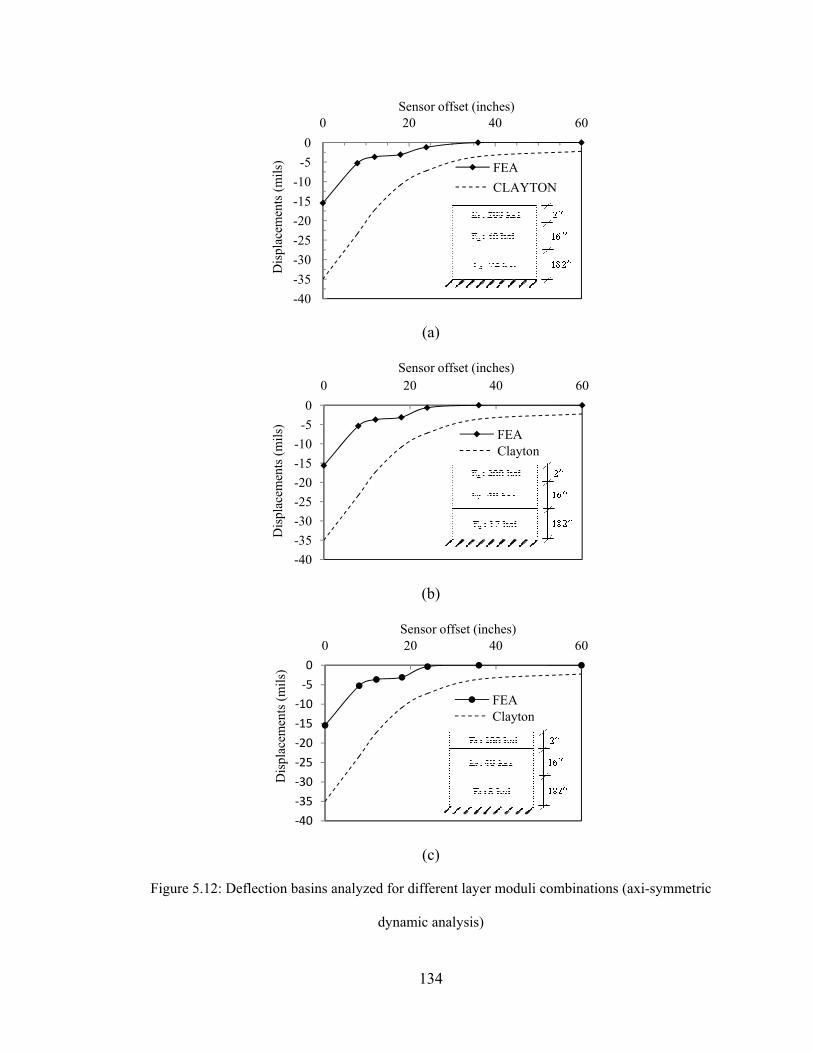
FFigure 5.12: DDeflection ba
-4-3-3-2-2-1-1-
Dis
plac
emen
ts (m
ils)
-4-3-3-2-2-1-1-
Dis
plac
emen
ts (m
ils)
‐4
‐3
‐3
‐2
‐2
‐1
‐1
‐
Dis
plac
emen
ts (m
ils)
asins analyzed
d
050505050
0
4050
2520
50
-50
0
40
35
30
25
20
15
10
‐5
0
0
134
(a)
(b)
(c)
d for different
dynamic anal
20Sensor offs
20Sensor offs
20Sensor offs
t layer moduli
ysis)
40set (inches)
FEACLAYT
40set (inches)
FEAClayto
40fset (inches)
FEAClayton
i combination
60
TON
60
n
60
n
ns (axi-symmmetric

FFigure 5.12: DDeflection ba
‐4
‐3
‐3
‐2
‐2
‐1
‐1
‐
Dis
plac
emen
ts (m
ils)
-4-3-3-2-2-1-1
-
Dis
plac
emen
ts (m
ils)
-4-3-3-2-2-1-1-
Dis
plac
emen
ts (m
ils)
asins analyzed
d
0
5
0
5
0
5
0
5
0
0
4050
2520
50
-50
0
4035302520
50
-50
0
135
(d)
(e)
(f)
d for different
dynamic anal
20Sensor offse
20Sensor offse
20Sensor off
t layer moduli
ysis)
40et (inches)
FEAClayton
40et (inches)
FEAClayto
40fset (inches)
FEAClayto
i combination
60
60
on
60
on
ns (axi-symmmetric

136
(a) E1: 200, E2: 40, E3: 24 ksi
(b) E1: 200, E2: 40, and E3: 17 ksi
(c) E1: 200, E2: 40, and E3:8 ksi
Figure 5.13: Time-deflection histories at the sensors for layer moduli combinations (axi-
symmetric dynamic analysis)
-20
-15
-10
-5
0
5
0 10 20 30 40 50 60
Dis
plac
emen
ts (m
ils)
Time (milli seconds)
D1D2D3D4D5D6D7
‐20
‐15
‐10
‐5
0
5
0 10 20 30 40 50 60
Dis
plac
emen
t (m
ils)
Time (milli seconds)
D1D2D3D4D5D6D7
‐20
‐15
‐10
‐5
0
5
0 10 20 30 40 50 60
Dis
plac
emen
t (m
ils)
Time (milli seconds)
D1D2D3D4D5D6D7

137
(d) E1: 300, E2: 40, and E3: 24 ksi
(e) E1: 300, E2: 40, and E3: 17ksi
(f) E1: 300, E2: 40, and E3: 8 ksi
Figure 5.13: Time-deflection histories at the sensors for layer moduli combinations (axi-
symmetric dynamic analysis)
‐20
‐15
‐10
‐5
0
5
0 20 40 60 80 100
Dis
plac
emen
ts (m
ils)
Time (milli seconds)
D1D2D3D4D5D6D7
-20
-15
-10
-5
0
5
0 20 40 60 80 100
Dis
plac
emen
ts (m
ils)
Time (milli seconds)
D1D2D3D4D5D6D7
-20
-15
-10
-5
0
5
0 20 40 60 80 100
Dis
plac
emen
ts (m
ils)
Time (milli seconds)
D1D2D3D4D5D6D7

Figure 5.14:: Deflection b
-4-3-3-2-2-1-1
-
Dis
plac
emen
ts (m
ils)
-4-3-3-2-2-1-1
Dis
plac
emen
ts (m
ils)
-4-3-3-2-2-1-1
Dis
plac
emen
ts (m
ils)
basins analyze
d
40353025201510-50
0
40353025201510-50
0
40353025201510-50
0
138
(a)
(b)
(c)
ed for differen
dynamic anal
20Sensor offse
20Sensor offs
20Sensor of
nt layer modu
ysis)
40et (inches)
FEAClay
40set (inches)
FEACla
40ffset (inches)
FECla
uli combinatio
60
Ayton
60
Aayton
60
Aayton
ons (quarter ccube
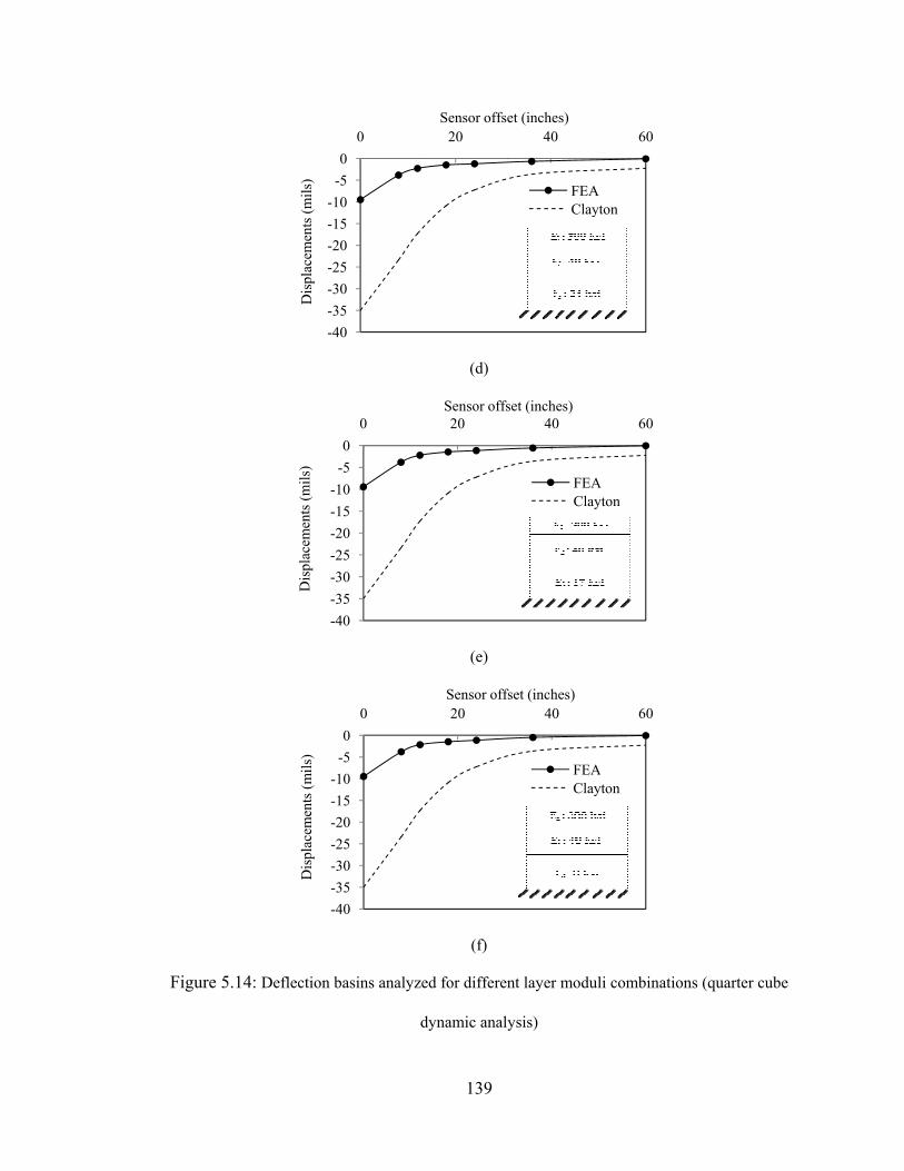
Figure 5.14:: Deflection b
-4-3-3-2-2-1-1
-
Dis
plac
emen
ts (m
ils)
-4-3-3-2-2-1-1
Dis
plac
emen
ts (m
ils)
-4-3-3-2-2-1-1
Dis
plac
emen
ts (m
ils)
basins analyze
d
4035302520
50
-50
0
40353025201510-50
0
40353025201510-50
0
139
(d)
(e)
(f)
ed for differen
dynamic anal
20Sensor offs
20Sensor offs
20Sensor off
nt layer modu
ysis)
40et (inches)
FEAClay
40set (inches)
FEACla
40fset (inches)
FEACla
uli combinatio
60
Ayton
60
Aayton
60
Aayton
ons (quarter ccube

140
(a) E1: 200, E2: 40, and E3: 24 ksi
(b) E1: 200, E2: 40, and E3: 17 ksi
(c) E1: 200, E2: 40, and E3: 8 ksi
Figure 5.15: Time-deflection histories at the sensors for layer moduli combinations (quarter cube
dynamic analysis)
-10
-8
-6
-4
-2
0
2
0 20 40 60 80 100
Dis
plac
emen
t (m
ils)
Time (milli seconds)
D1D2D3D4D5D6D7
-10
-8
-6
-4
-2
0
2
4
0 20 40 60 80 100
Dis
plac
emen
t (m
ils)
Time (milli seconds)
D1D2D3D4D5D6D7
-12
-10
-8
-6
-4
-2
0
2
0 20 40 60 80 100
Dis
plac
emen
t (m
ils)
Time (milli seconds)
D1D2D3D4D5D6D7

141
(d) E1: 300, E2: 40, and E3: 24 ksi
(e) E1: 300, E2: 40, and E3: 17 ksi
(f) E1: 300, E2: 40, and E3: 8 ksi
Figure 5.15: Time-deflection histories at the sensors for layer moduli combinations (quarter cube
dynamic analysis)
-12
-10
-8
-6
-4
-2
0
2
0 20 40 60 80 100
Dis
plac
emen
t (m
ils)
Time (milli seconds)
D1D2D3D4D5D6D7
-12
-10
-8
-6
-4
-2
0
2
0 20 40 60 80 100
Dis
plac
emen
t (m
ils)
Time (milliseconds)
D1D2D3D4D5D6D7
-12
-10
-8
-6
-4
-2
0
2
0 20 40 60 80 100
Dis
plac
emen
t (m
ils)
Time (milli seconds)
D1D2D3D4D5D6D7

142
(a) Static analysis
(b) Dynamic analysis
Figure 5.16: Contour of vertical deflection (200, 40, and 8 ksi)

143
(a) Static analysis
(b) Dynamic analysis
Figure 5.17: Contour of vertical deflection (300, 40, and 24 ksi)
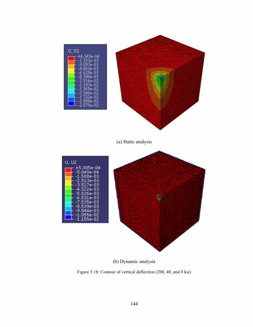
144
(a) Static analysis
(b) Dynamic analysis
Figure 5.18: Contour of vertical deflection (200, 40, and 8 ksi)

145
(a) Static analysis
(b) Dynamic analysis
Figure 5.19: Contour of vertical deflection (300, 40, and 24 ksi)

146
(a) Static analysis
(b) Dynamic analysis
Figure 5.20: Contour of von Mises stress (200, 40, and 8 ksi)

147
(a) Static analysis
(b) Dynamic analysis
Figure 5.21: Contour of von Mises stress (300, 40, and 24 ksi)

148
(a) Static analysis
(b) Dynamic analysis
Figure 5.22: Contour of von Mises stress (200, 40, and 8 ksi)
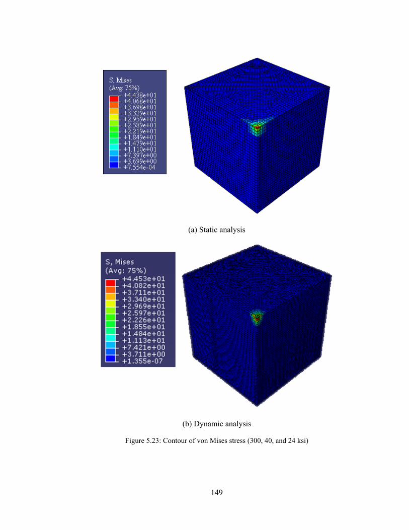
149
(a) Static analysis
(b) Dynamic analysis
Figure 5.23: Contour of von Mises stress (300, 40, and 24 ksi)
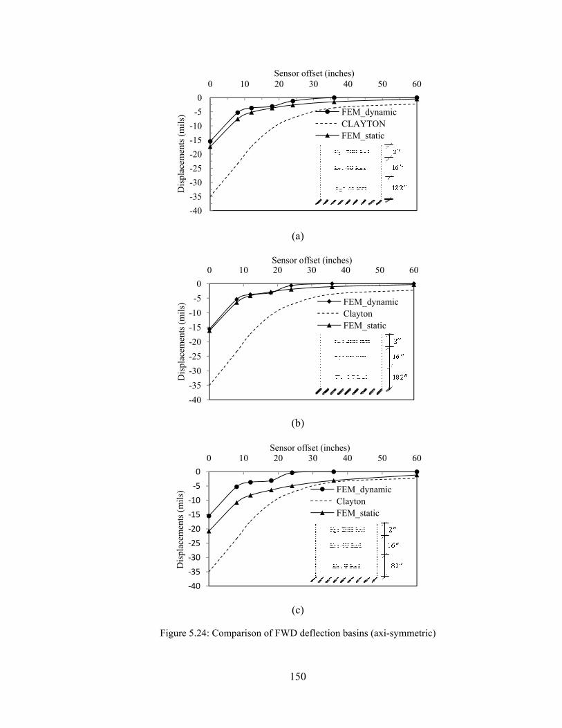
Figure 5.24:
-40-35-30-25-20-15-10
-50
0
Dis
plac
emen
ts (m
ils)
-40-35-30-25-20-15-10
-50
0
Dis
plac
emen
ts (m
ils)
‐40
‐35
‐30
‐25
‐20
‐15
‐10
‐5
0
0
Dis
plac
emen
ts (m
ils)
Comparison
0 10
0 10
0 10
150
(a)
(b)
(c)
of FWD defl
20 30Sensor offs
20 30Sensor offse
20 30Sensor offse
ection basins
0 40set (inches)
FEM_dCLAYTFEM_s
0 40et (inches)
FEM_dClaytonFEM_s
0 40t (inches)
FEM_dyClaytonFEM_sta
(axi-symmet
50 60
dynamicTONstatic
50 60
dynamicnstatic
50 60
ynamic
atic
tric)
0
0

Figure 5.24:
‐40
‐35
‐30
‐25
‐20
‐15
‐10
‐5
0
0
Dis
plac
emen
ts (m
ils)
‐40
‐35
‐30
‐25
‐20
‐15
‐10
‐5
0
0
Dis
plac
emen
ts (m
ils)
‐40
‐35
‐30
‐25
‐20
‐15
‐10
‐5
0
0
Dis
plac
emen
ts (m
ils)
Comparison
0
0
0 10
151
(d)
(e)
(f)
of FWD defl
20Sensor offs
20Sensor offs
20 30Sensor offset
ection basins
40set (inches)
FEM_dClaytoFEM_s
40set (inches)
FEM_dClaytonFEM_st
0 40t (inches)
FEM_dClaytonFEM_s
(axi-symmet
60
dynamicnstatic
60
dynamicntatic
50 60
dynamicnstatic
tric)

Figure 5.25
-40-35-30-25-20-15-10-50
0
Dis
plac
emen
ts (m
ils)
-40-35-30-25-20-15-10-50
0
Dis
plac
emen
ts (m
ils)
-40-35-30-25-20-15-10-50
0
Dis
plac
emen
ts (m
ils)
: Comparison
0
0
0 10
152
(a)
(b)
(c)
n of FWD def
20Sensor offs
20Sensor off
20 30Sensor off
flection basin
40set (inches)
FEMClayFEM
40fset (inches)
FEM_ClaytFEM_
0 40fset (inches)
FEM_ClaytoFEM_
ns (quarter cub
60
M_dynamicytonM_static
60
_dynamicton_static
50 60
_staticon_dynamic
be)

Figure 5.25
-40-35-30-25-20-15-10-50
0
Dis
plac
emen
ts (m
ils)
-40-35-30-25-20-15-10-50
0
Dis
plac
emen
ts (m
ils)
-40
-35
-30
-25
-20
-15
-10
-5
00
Dis
plac
emen
ts (m
ils)
: Comparison
0 10
0 10
0 10
153
(d)
(e)
(f)
n of FWD def
20 30Sensor offs
20 30Sensor off
20 30
Sensor off
flection basin
0 40set (inches)
FEM_ClaytoFEM_
0 40fset (inches)
FEMClaytFEM
0 40
fset (inches)
FEM_ClaytoFEM_
ns (quarter cub
50 60
_staticon_dynamic
50 60
M_dynamicton
M_static
50 60_dynamicon_static
be)

154
CHAPTER 6
CONCLUSIONS
This study evaluates most widely used FWD software based on accuracy and consistency
to back-calculate the modulus of elasticity of the airport pavements in New Mexico.
These software are BAKFAA, MODULUS 6.0 and EVERCALC. The purpose was to
find software that can back calculate the pavement layer moduli most accurately and
consistently from the FWD test data.
To check the accuracy, the back calculated moduli of the surface course from the
aforementioned software are compared to the resilient modulus of the asphalt concrete
from laboratory testing. The indirect tensile strength test of asphalt concrete was also
performed and then, the tensile stress at the bottom (determined by KENLAYER, a multi
layered elastic analysis software) is compared to the laboratory indirect tensile strength of
asphalt concrete to investigate the accuracy. For the further investigation of the accuracy,
the back calculated subgrade modulus is compared to the field modulus determined from
CBR values using the CBR-modulus empirical relationship. During the field FWD test,
each and every point on the airfield was tested under three different loads and they are 9,
12, and 16 kips.
To check the consistency of the analysis results from the software, the coefficient of
variation (CV) of the back calculated layer moduli at these test loads is determined at
every test station. The frequency distribution of the CV is then plotted to find the
software that gives least variation in analysis results. For this study, FWD data were
collected from seven different runways and they are Runway 4-22 of Double Eagle II,

155
Runway 12-30 of Sierra Blanca Regional, Runway 2-20 and 7-25 of Raton Municipal,
Runway 8-26 of Las Cruces, Runway 8-26 of Moriarty, Runway 8-26 of Silver city
airport. The asphalt cores and soil samples are also collected from these runways.
The aforementioned software are based on the multi-layered elastic theory and for this
reason, during analysis the pavement layers are assumed as linear elastic. But in reality,
pavement response can not always be elastic. Therefore, for the better prediction of the
pavement characteristics under FWD test, the dynamic analysis of the multi layered
flexible pavement was performed by finite element method. The stress-strain distribution
of the layer material was assigned as the layer properties of the FEM model. FEM
analysis includes two different geometries. The first one is axi-symmetric and the second
one is quarter cube model. The pavement response is analyzed in response to the impulse
loading. To apply the impulse on the model, the time-load history data is used from FWD
test from Clayton airport. The predicted time-deflection histories are then compared to
the field response in terms of the peak deflection, the time of occurrence of the peak
values, and their time lag.
Based on the studies mentioned above the conclusions can be summarized as follows:
The consistency of FWD backcalculation software is evaluated using frequency
distributions of the backcalculated moduli and CV of moduli from an identical
location tested at three levels of FWD loads. For surface modulus, variation in
modulus and CV of EVERCALC software are slightly higher than those of
MODULUS software. The base modulus variation is the least in EVERCALC.
For subgrade modulus, EVERCALC is more consistent than BAKFAA and
156
MODULUS. Overall, the variation is highest in BAKFAA, and MODULUS
ranked second. EVERCALC is the most consistent backcalculation software for
determining runway pavement layer moduli.
The accuracy of the backcalculated surface modulus is examined by comparing
backcalculated modulus to the laboratory resilient modulus. It is shown that
EVERCALC produces modulus values closer to the laboratory resilient modulus
compared to MODULUS and BAKFAA software. The backcalculated tensile
strength is compared to the laboratory indirect tensile strength of the asphalt core
and it is observed that EVERCALC is more appropriate than MODULUS and
BAKFAA software. The comparison of the backcalculated subgrade modulus to
the laboratory subgrade modulus has shown that backcalculated subgrade
modulus from EVERCALC is more close to the laboratory value than that from
MODULUS and BAKFAA software.
For the same combination of layer moduli, the axi-symmetric and quarter cube
geometries yield different analysis results. The axi-symmetric model shows
higher deflections than that from quarter cube model. The peak deflections from
the axi-symmetric model are closer to the field FWD data for the mentioned
moduli combinations.
From the field FWD data, it is observed that the response of the flexible pavement
under the impulse is instantaneous and the time lags between the successive
sensors are very small. In this study, the analyses show the significant amount of
time lag between the two successive points and also the time of occurrence of the
higher than that of the field data in both of the two different geometries.

157
For the variation of the combinations of the layer moduli, the surface modulus is
varied from 200 to 300 ksi and the subgrade modulus is varied from 17 to 40 ksi.
The base modulus is kept constant. The analysis results have shown that these
combinations does not affect significantly.
The static deflection is greater than the dynamic deflection and closer to the field
FWD deflection basin. The deflection in static analysis is more sensitive to the
layer modulus variation than the dynamic analysis.
The following points can be recommended for the future studies:
The surface course in the finite element modeling was assumed linear elastic in
this study. The non linear stress-strain distribution may be more appropriate to
address the accurate behavior of the asphalt concrete.
The models developed in this study, is analyzed for only one test point on the
runway 12-30 of Clayton airport. More data points can be used for rigorous
validation of the model.
Also more combination of material properties can be tried in FEM analysis.
The laboratory testing can be conducted on soil and aggregate to determine the
actual modulus of elasticity of subgrade and base layer as well as to obtain the
proper stress-strain distribution of the layer material that can be used for the finite
element modeling.
158
REFERENCES
Ameri, M., Yavari, N. and Scullion, T. (2009). “Comparison of Static and Dynamic
Backcalculation of Flexible Pavement Layers Moduli, using four softwares.” Asian
Journal of Applied Sciences, Vol. 2, No. 3, pp. 197-210.
American Association of State Highway and Transportation Officials. (1993). AASHTO
Guide for Design of Pavement Structures: Rehabilitation Method with Overlays,
Washington D.C.
ASTM D 2487. (2000)“Standard Practice for Classification of Soils for Engineering
Purposes (Unified Soil Classification System).” Construction: Soil and Rock (I), Vol.
04.08, 100 Barr Drive, West Conshohocken, PA 19428.
ASTM D 3080 – 04. “Standard Test Method for Direct Shear Test of Soils under
Consolidated Drained Conditions.”
ASTM D 4123-82. (1995). “Standard Test Method for Indirect Tension Test for Resilient
Modulus of Bituminous Mixtures.”
ASTM D 4694-96. (1996). “Standard Test Method for Deflections with a Falling Weight-
Type Impulse Load Device”, Annual Book of ASTM Standards, Volume 04.03, Road
and Paving Materials; Paving Management Technology.
Boussinesq, J. (1885). “Application des potential a l’ etude de l’ equilibre et du
mouvement des solides elastigue”.
Burmister, D. M. (1943). “The Theory of Stresses and Displacement in Layered Systems
and Applications to the Design of Airport Runways,” Proceedings, Highway Research
Board , Vol.23, pp.126-144.
Burmister, D. M. (1945). “The General Theory of Stresses and Displacements in Layered
Soil Systems.” Journal of Applied Physics, Vol. 16, pp. 84-94.

159
Cho, Y. H., McCullough, B. F., and Weissmann, J. (1997). “Considerations on Finite
Element method Application in Pavement Structural Analysis.” Transportation
Research Record, vol. 1539, pp.96-101.
Das, B. M. (1983). Advanced Soil Mechanics. Hemisphere Publishing Corporation, USA.
Dunlop, P., Duncan, J. M., and Seed, H. B. (1970). “Finite Element Analysis of Slopes in
Soil.” Journal of the Soil Mechanics and Foundations Division, Proceedings of
American Society of Civil Engineers, 96(2).
Everseries User’s Guide. “Pavement analysis computer software and case studies.”
<<http://wsdot.wa.gov/biz/mats/pavement/EVERSERS/EverseriesUserguide.pdf>>
(2005).
Federal Aviation Administration (FAA). (2002). Advisory Circular No. 150/5370-11A,
“Use of Non Destructive Testing in the Evaluation of Airport Pavements.”
Garg, N. and Thompson, M. R. (1997). “Triaxial Characterization of Minnesota Road
Research Project Granular Materials.” Transportation Research Record 1577, pp. 27-
36.
Göktepe, A. B., Aĝar, E. and Lav, A. H. (2004). “Comparison of Multilayer Perceptron
and Adaptive Neuro-Fuzzy System on Backcalculating the Mechanical Properties of
Flexible Pavements.” ARI The Bulletin of the Istanbul Technical University,Vol. 54,
Num. 3, (Received Dec. 31, 2004)
Gopalakrishnan, K., and Thompson, M.R. (2007). “Characterization of NAPTF subgrade
soils for mechanistic-based analysis and design of airport flexible pavements.”
International Journal of Pavement Engineering, 8(4), pp. 307-321.
160
Haddad, Y. M. (1995). “Viscoelasticity of Engineering Materials.” 1st edition, Chapman
& Hall, pp. 33-34.
Heukelom, W. and Klomp, A.J.G. (1962). “Dynamic Testing as a means of controlling
pavements during and after construction.” Proceedings of the First International
Conference on Structural Design of Asphalt Pavements, University of Michigan, Ann
Arbor.
Hibbeler, R. C. (2005). Mechanics of Materials. 6th Ed. Pearson Prentice Hall. Pearson
Education Inc. Upper Saddle River, NJ.
Hjelmstad, K. D., Zuo, Q., and Kim, J. (1997). “Elastic Pavement Analysis Using Infinite
Elements.” Transportation Research Record, Vol. 1568, pp. 72-76.
Hoffman, M. S. (1983). “Loading Mode Effects on Pavement Deflections.” Journal of
Transportation Engineering, ASCE, 109 (5), pp. 651-667.
Huang, Y. H. (2004). Pavement Analysis and Design, 2nd Ed. Pearson Prentice Hall.
Pearson Education Inc. Upper Saddle River, NJ.
Huang, Y. H. (2004). “Stresses and Displacements in Nonlinear Soil Media.” Journal of
the Soil Mechanics and Foundation Division, ASCE, Vol. 94, pp. 1-19.
Irwin, L. H. “Backcalculation: An Overview and Perspective.”
<http://pms.nevadadot.com/2002.asp> (2002).
Ji, Y., Wang, F., Luan, M. and Guo, Z. (2006). “A Simplified for Dynamic Responses of
Flexible Pavement and Applications in Time domain Backcalculation.” The Journal of
American Science,Vol. 2, No.2.

161
Khazanovich, L. and Wang, Q. (2007). “MnLayer High-Performance Layered Elastic
Analysis Program.” Transportation Research Record: Journal of the Transportation
Research Board, No. 2037, pp. 63-75.
Koswara, H. (1983). “A Finite Element Analysis of Underground Shelter Subjected to
Ground Shock Load.” M. S. Thesis, Rose-Hulman Institute of Technology, Terre
Haute, IN.
Kuo, C. M., and Chou, F. J. (2004). “Development of 3-D Finite Element Model For
Flexible Pavements.” Journal of the Chinese Institute of Engineers, 27(5), pp. 707-
717.
Larkin, A. and Hayhoe, G. F. (2009). “Federal Aviation Administration Airport
Pavement Management and Airport Pavement Roughness Evaluation.” Non-
Destructive Testing in Civil Engineering, Nantes, France.
Logan, D. L. (2007). A First Course in the Finite Element Method. 4th Edition, Thomson
Canada Limited.
Love, A. E. H. (1927). “Mathematical theory of elasticity.” 4th ed., Cambridge University
Press, Cambridge, U.K.
Lukanen, E. O. (1993). “Effects of buffer on falling weight deflectometer loadings and
deflections.” Transportation Research Record, 1355, pp. 37-51.
Lytton, R. L., Uzan, J., Fernando, E. G., Roque, R., Hiltunen, D., and Stoffels, S. M.
(1993). “Development and Validation of Performance Prediction Models and
Specifications for Asphalt Binders and Paving Mixes.” Report SHRP-A-357 Strategic
Highway Research Program, National Research Council, Washington, D. C.

162
Mahoney, J. P., Coetzee, N. F., Stubstad, R. N. and Lee, S. W. (1989). “A Performance
Comparison of Selected Backcalculation Computer Programs.” Nondestructive
Testing of Pavements and Backcalculation of Moduli, American Society for Testing
and Materials (ASTM), STP 1026, pp. 470-486.
MEPDG. “Guide for Mechanistic-Empirical design of new and rehabilitated pavement
structures.” <http://www.trb.org/mepdg/2appendices_cc.pdf> (2008).
MEPDG. (2008), “Mechanistic-Empirical Pavement Design Guide”, Interim Edition, pp.
126.
Nam, D. (1994). “Effect on Slab Flexibility on the Vertical Stiffness of Circular
Foundations.” M.S. thesis. University of Texas at Austin.
Nazarian, S. and Boddapati, K. M. (1995). “Pavement-falling weight deflectometer
interaction using dynamic finite element analysis.” Transportation Research Record,
1482, pp. 33-43.
NCHRP. <<Mechanistic-Empirical Design of New and Rehabilitated Pavement
Structures.>> National Cooperative Highway Research Program, NCHRP Project 1-
37A Report, National Research Council, Washington, D.C., 2004.
Odemark, N. (1949).” Investigation as to the Elastic Properties of Soils and Design of
pavements According to the Theory of Elasticity,” Meddlande 77, Statens Vaginstitut;
Stockholm, Sweden.
Press, W. H., Teukolsky, S. A., Vetterling, W. T. and Flannery, B. P. (2007).
NUMERICAL RECIPES: The Art of Scientific Computing, 3rd Ed. Cambridge
University Press, Cambridge.

163
Rahim, A. and George, K. P. (2003). “Falling Weight Deflectometer for Estimating
Subgrade Elastic Modulus.” Journal of Transportation Engineering, ASCE, 129(1),
pp. 100-107.
Roesset, J. M., Stokoe II, K. H., and Seng, C. R. (1995). “Determination of depth to
bedrock from falling weight deflectometer test data.” Transportation Research
Record: Journal of the Transportation Research Board, No. 1504, pp. 68-7.
Romanoschi, S., and Metcalf, J. B. (1999). “Simple Approach to Estimation of Pavement
Structural Capacity.” Transportation Research Record, vol. 1652, pp. 198-205.
Saltan, M. (2002). “Modeling Deflection Basin Using Neurofuzzy in Backcalculating
Flexible Pavement Layer Moduli.” Pakistan Journal of Information and Technology
1(2): 180-187.
Sebaaly, B. E., Mamlouk, M. S., and Davies, T. G. (1986). “Dynamic analysis of falling
weight deflectometer data.” Transportation Research Record, Vol. 1070, pp. 63-68.
Slope Stability. (2003). “Engineering and Design – Slope Stability.” US Army Corps of
Engineers, Engineering and Design, EM 1110-2-1902, Chap. 4, pp. 1-16.
Tarefder, R. A, Stormont, J. C., and Zaman, M. M. (2007). "Evaluating Laboratory
Modulus and Rutting of Asphalt Concrete." Compendium of CR-ROM Papers, 86th
Annual Meeting of TRB, Washington D.C., Paper No 07-1889.
Thompson, M. R. (1982). “ILLI-PAVE, Users Manual.” Transportation Research
Facilities, Department of Civil Engineering, University of Illinois, Urbana.
Timoshenko, S. P., and Goodier, J. N. (1970). “Theory of Elaticity.” 3rd ed., McGraw-
Hill Book Co., New York, N.Y.

164
Uddin, W., Hackett, R. M., Joseph, A. P., Algred, B. (1995). “Three-Dimensional Finite-
Element Analysis of Jointed Concrete Pavement with Discontinuities.” Transportation
Research Record, vol. 1482, pp. 26-32.
Uddin, W., and McCullough, B. F. (1989). “In Situ Material Properties from Dynamic
Deflection Equipment.” Nondestructive Testing of Pavements and Backcalculation of
Moduli, American Society for Testing and Materials (ASTM), STP 1026, pp. 278-290.
Uzan, J., Lytton, R. L., and Germann, F. P. (1989). “General Procedure for
Backcalculating Layer Moduli.” Nondestructive Testing of Pavements and
Backcalculation of Moduli, ASTM STP 1026, pp. 217-228.
Van Metzinger, W. A., McCullough, B. F. (1991). “An Empirical-Mechanistic Design
Method Using Bonded Concrete Overlays for the Rehabilitation of Pavements.”
Center for Transportation Research, University of Texas at Austin, Report 1205-1.
William, G. W. (1999).“Backcalculation of pavement layers moduli using 3D nonlinear
explicit finite element analysis.” M.Sc. Thesis, West Virginia University, West
Virginia, USA.
Witczak, M.W., Qi, X. and Mirza, M.W. (1995). “Use of Nonlinear Subgrade Modulus in
AASHTO Design Procedure.” Journal of Transportation Engineering, ASCE, Vol.
121, No. 3, pp. 273-282.
Wood, D. M. (1990). Soil Behaviour and Critical State Soil Mechanics. Cambridge
University Press.
Wu, C., Y., Liu, X., Y., Scarpas, A. and Ge, X., R. (2006). “Spectral Element Approach
for Forward Models of 3D Layered Pavement.” CMES, Vol.12, No.2, PP.149-157.

165
Yamada, Y. (1970). “Dynamic Analysis of Civil Engineering Structures.” Recent
Advances in Matrix Methods of Structural Analysis and Design, University of
Alabama Press, Tuscaloosa, AL, pp. 487-512.
Yin, D. and Mrawira, D. (2009). “Comparison between Laboratory Investigation and
Non-Destructive Testing Methods for Mechanistic Characterization of Asphalt
Pavement.” 88th Annual Meeting of Transportation Research Board, Vol. 09, No.
3339.

166
APPENDICES
Contour of Vertical Deflection
(a) Static analysis
(a) Dynamic analysis
Figure 1: Contour of vertical deflection (200, 40, and 17 ksi)

167
(a) Static analysis
(b) Dynamic analysis
Figure 2: Contour of vertical deflection (200, 40, and 24 ksi)

168
(a) Static analysis
(b) Dynamic analysis
Figure 3: Contour of vertical deflection (300, 40, and 8 ksi)

169
(a) Static analysis
(b) Dynamic analysis
Figure 4: Contour of vertical deflection (300, 40, and 17 ksi)

170
(a) Static analysis
(b) Dynamic analysis
Figure 5: Contour of vertical deflection (200, 40, and 17 ksi)

171
(a) Static analysis
(b) Dynamic analysis
Figure 6: Contour of vertical deflection (200, 40, and 24 ksi)

172
(a) Static analysis
(b) Dynamic analysis
Figure 7: Contour of vertical deflection (300, 40, and 8 ksi)

173
(a) Static analysis
(b) Dynamic analysis
Figure 8: Contour of vertical deflection (300, 40, and 17 ksi)

174
Contour of von Mises Stress
(a) Static analysis
(b) Dynamic analysis
Figure 1: Contour of von Mises stress (200, 40, and 17 ksi)

175
(a) Static analysis
(b) Dynamic analysis
Figure 2: Contour of von Mises stress (200, 40, and 24 ksi)
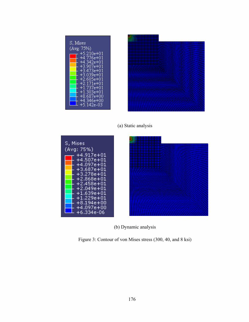
176
(a) Static analysis
(b) Dynamic analysis
Figure 3: Contour of von Mises stress (300, 40, and 8 ksi)
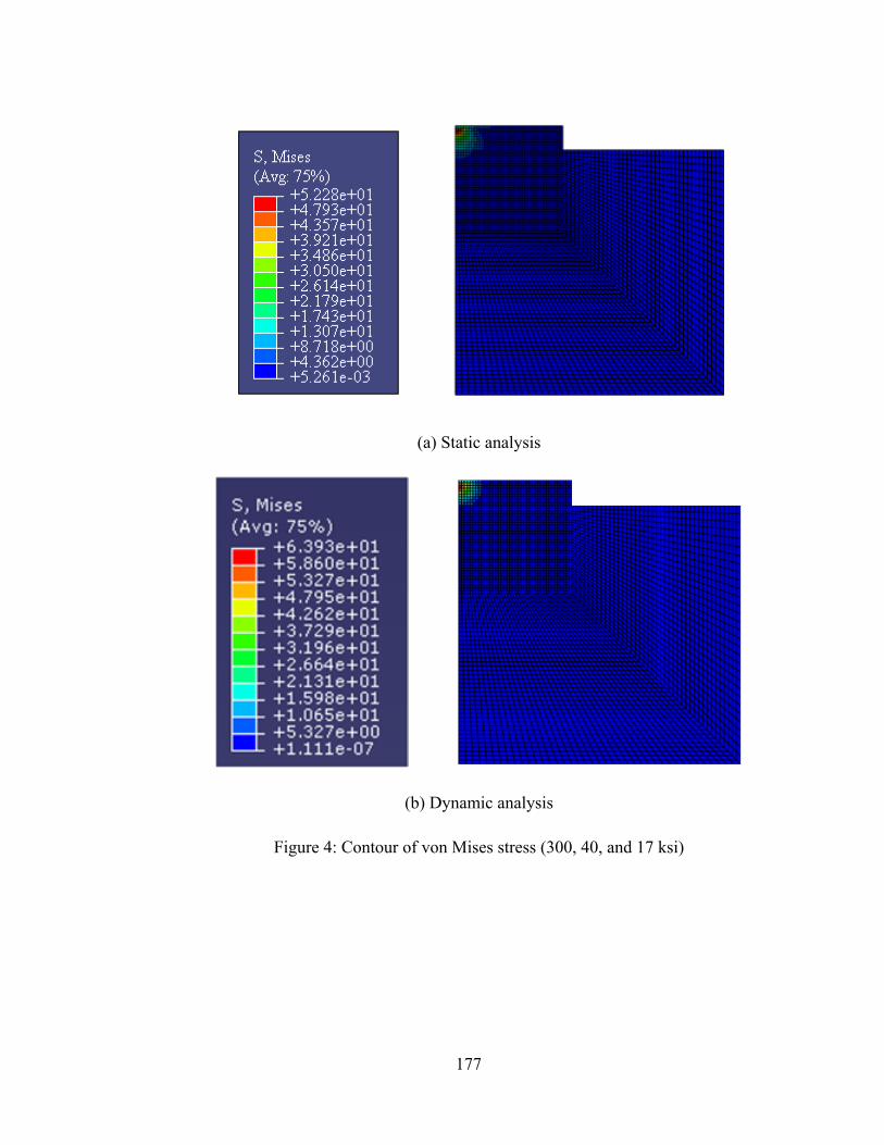
177
(a) Static analysis
(b) Dynamic analysis
Figure 4: Contour of von Mises stress (300, 40, and 17 ksi)

178
(a) Static analysis
(b) Dynamic analysis
Figure 5: Contour of von Mises stress (200, 40, and 17 ksi)

179
(a) Static analysis
(b) Dynamic analysis
Figure 6: Contour of von Mises stress (200, 40, and 24 ksi)

180
(a) Static analysis
(b) Dynamic analysis
Figure 7: Contour of von Mises stress (300, 40, and 8 ksi)

181
(a) Static analysis
(b) Dynamic analysis
Figure 8: Contour of von Mises stress (300, 40, and 8 ksi)