Evaluation of extreme learning machine for classification...

Accepted Manuscript

Evaluation of extreme learning machine for classification of individualand combined finger movements using electromyography on amputeesand non-amputees

Khairul Anam, Adel Al-Jumaily

PII: S0893-6080(16)30131-9DOI: http://dx.doi.org/10.1016/j.neunet.2016.09.004Reference: NN 3666

To appear in: Neural Networks

Received date: 17 January 2016Revised date: 17 July 2016Accepted date: 7 September 2016

Please cite this article as: Anam, K., & Al-Jumaily, A. Evaluation of extreme learning machinefor classification of individual and combined finger movements using electromyography onamputees and non-amputees. Neural Networks (2016),http://dx.doi.org/10.1016/j.neunet.2016.09.004

This is a PDF file of an unedited manuscript that has been accepted for publication. As aservice to our customers we are providing this early version of the manuscript. The manuscriptwill undergo copyediting, typesetting, and review of the resulting proof before it is published inits final form. Please note that during the production process errors may be discovered whichcould affect the content, and all legal disclaimers that apply to the journal pertain.

http://dx.doi.org/10.1016/j.neunet.2016.09.004

Evaluation of Extreme Learning Machine for Classification of

Individual and Combined Finger Movements using Electromyography

on Amputees and Non-amputees

Khairul Anam a,b,*, Adel Al-Jumailya

a University of Technology, Sydney, 15 Broadway Ultimo NSW Australia 2007 b University of Jember, 47 Kalimantan St, Jember, Indonesia 65168

Corresponding Authors:

Khairul Anam

[email protected]

Faculty of Engineering and Information

University of Technology, Sydney

Building 11 Room W9.205.20

15 Broadway, Ultimo NSW 2007 Australia

+61 2 9514 7959

Evaluation of Extreme Learning Machine for Classification of Individual and Combined Finger Movements using Electromyography on Amputees and Non-

amputees

Khairul Anam a,b,*, Adel Al Jumailya

a University of Technology, Sydney, 15 Broadway Ultimo NSW Australia 2007

b University of Jember, 47 Kalimantan St, Jember, Indonesia 65168

Abstract

The success of myoelectric pattern recognition (M-PR) mostly relies on the features extracted and

classifier employed. This paper proposes and evaluates a fast classifier, extreme learning machine

(ELM), to classify individual and combined finger movements on amputees and non-amputees. ELM

is a single hidden layer feed-forward network (SLFN) that avoid iterative learning by determining

input weights randomly and output weights analytically. Therefore, it can accelerate the training time

of SLFNs. In addition to the classifier evaluation, this paper evaluates various feature combinations to

improve the performance of M-PR and investigate some feature projections to improve the class

separability of the features. Different from other studies on the implementation of ELM in the

myoelectric controller, this paper presents a complete and thorough investigation of various types of

ELMs including the node-based and kernel-based ELM. Furthermore, this paper provides

comparisons of ELMs and other well-known classifiers such as linear discriminant analysis (LDA), k-

nearest neighbour (kNN), support vector machine (SVM) and least-square SVM (LS-SVM). The

experimental results show the most accurate ELM classifier is radial basis function ELM (RBF-

ELM). The comparison of RBF-ELM and other well-known classifiers shows that RBF-ELM is as

accurate as SVM and LS-SVM but faster than the SVM family; it is superior to LDA and kNN. The

experimental results also indicate that the accuracy gap of the M-PR on the amputees and non-

amputees is not too much with the accuracy of 98.55% on amputees and 99.5% on the non-amputees

using six electromyography (EMG) channels.

* Corresponding author Email: [email protected]

2

Keyword: Classification, myoelectric pattern recognition, electromyography (EMG), extreme learning machine (ELM), amputee

1. Introduction

A hand disability is one of the most frequent disability problems that occur in the community. The

hand disability can be caused by either amputation or a motor function problem. The development of

the perfect technology for hand rehabilitation is a challenging task. Various cutting-edge technologies

have been developed to deal with the hand rehabilitation. For hand amputees, Touch Bionics Limited

has introduced a revolutionary prosthetic hand named iLimb (TouchBionics, 2007). The iLimb looks

like a natural hand, and it is designed in such a way that it conforms around the shape of an object

being grasped. I-LIMB has five fingers so that it can perform a large number of finger configurations.

Another example of a bionic hand that is available in the market is a bebionic hand by RSLSteeper

(Scheme & Englehart, 2011). Thus, the hardware of the robotic hands that mimic the hand in the

shape and functionality are available. These sophisticated prosthetic hands need a sophisticated

control system that can be applied in the real-time application. In addition, the control system should

work in agreement with a human’s desire to enhance the convenience of the wearer. A so-called

myoelectric control system (MCS) which utilized a pattern-recognition method can be employed to

meet the demands of the control system on the dexterous prosthetic hand (Oskoei & Hu, 2007).

Feed-forward neural networks (FFNNs) or multi-layer perceptron (MLP) have become a popular

classifier in the field of myoelectric pattern recognition system (M-PR). To the best of the authors’

knowledge, Uchida, Hiraiwa, Sonehara, and Shimohara (1992) were the first researchers

implementing FFNNs on the M-PR for finger movement classification. In the proposed system,

FFNNs processed fast Fourier transform (FFT) features extracted from two electromyography (EMG)

channels. Using this system, they could classify five-finger movement with an accuracy of about 86%.

Fourteen years later, Tsenov, Zeghbib, Palis, Shoylev, and Mladenov (2006) proposed and developed

a myoelectric recognition system using multilayer perceptron (MLP) for finger movement cases. MLP

classified four finger movements using time-domain (TD) feature and achieved an accuracy of 93%

using two EMG channels and 98% using four EMG channels. In addition to the researchers above,

3

Tenore et al. (2009) employed MLP in their pattern recognition system. Different from previous

approaches that worked on healthy subjects only, the system was also applied to the amputees. The

system could recognize individual finger flexion and extension by the accuracy of on average 90 %.

The result also showed that the accuracy between the amputee and the able-bodied subjects is not

significantly different.

The classical problems of the artificial neural networks (ANNs), which need a heuristic

architectural process and take much training time, encourage the researchers to find alternative

classifiers. Cipriani et al. (2011) utilized k-nearest neighbour (k-NN) as a classifier in their M-PR.

The proposed M-PR extracted features using time domain features (TD) from nine EMG channels on

five able-bodied subjects and five amputees. The experimental results showed that the system could

classify seven finger movements with an accuracy of around 79 % and 89 % on the amputees and

non-amputees, respectively. In addition, k-NN has a faster processing time and easier setup than

ANNs.

In the recent decade, many researchers have been interested in support vector machine (SVM).

Some published works show that SVM is more powerful than ANNs and used widely in many areas

including myoelectric pattern recognition system (Khushaba, Kodagoda, Takruri, & Dissanayake,

2012; Oskoei & Hu, 2008). In a finger classification case, Khushaba et al. (2012) utilized SVM to

classify ten finger movements consisting of individual and combined movements. The proposed M-

PR extracted features using TD and autoregressive (AR) features from two EMG channels. The

proposed system succeeded in obtaining an accuracy of about 92% in the offline classification and

90% in the online classification.

The most recent study on the M-PR for finger movement classification favoured linear

discriminant analysis (LDA) over SVM as the classifier (Al-Timemy, Bugmann, Escudero, &

Outram, 2013). LDA classifier does not need a complicated training procedure like ANNs. Besides, it

is fast. In addition, its performance is comparable to ANNs (Hargrove, Englehart, & Hudgins, 2007).

In this system, Al-Timemy et al. (2013) extracted features from six EMG channels using TD and AR

4

features to classify 12 and 15 movement classes on six amputees and ten able-bodied subjects,

respectively. The system succeeded in achieving average accuracy of around 98% on the able-bodied

subjects and approximately 90% of the amputee subjects. However, there was a significant accuracy

gap between the able-bodied subjects and amputees.

Recent studies indicate that the researchers are getting interested in reemploying ANNs but in

different forms. It is extreme learning machine (ELM). ELM is a single hidden layer feed-forward

network (SLFN) that omits an iterative learning by using random weights in the hidden layer and

calculated weights in the output layer. To the best of the author’s knowledge, Park, Kim, and Oh

(2011) and Lee et al. (2011) were the first and the second researchers who initiated the

implementation of ELM in the M-PR for hand movement recognition. Shi, Cai, Zhu, Zhong, and

Wang (2013) also employed ELM along with the entropy features to recognize the hand and wrist

movements. In addition, Anam, Khushaba, and Al-Jumaily (2013) initiated the use of ELM for finger

movement recognition. Unfortunately, the reported works on ELM were applied to the able-bodied

subjects only.

This paper proposes and evaluates the implementation of various types of ELMs in the M-PR to

classify the individual and combined finger movements on the amputees and non-amputees. ELM

consists of two groups: the node-based and the kernel-based ELM. The node-based ELM depends on

the activation function of the node while the kernel-based ELM relies on the kernel function of the

hidden layer. This paper covers these two ELM groups. This paper presents the comparison of ELMs

and other well-known classifiers such as linear discriminant analysis (LDA), k-nearest neighbourhood

(kNN), support vector machine (SVM) and least-square SVM (LS-SVM).

In addition to the classifiers, this paper investigates the combinations of various time-domains

(TD) and autoregressive features to improve the performance of the M-PR. Not only that, this paper

investigates the several feature projections to improve the class separibilty to enhance the

classification performances.

5

Therefore, the contributions of this paper are firstly, it presents a deep and thorough investigation

on the performance of ELMs in the myoelectric pattern recognition on the amputees and non-

amputees. Secondly, it presents the observation on the features combination that can enhance the

classification performance along with ELM. Finally, the paper investigates the optimal feature

projections that can work with ELM to improve the performance of M-PR for the individual and

combined finger movements on the amputees and non-amputees.

The paper is organized as follows. The next section presents the methodology consisting of the

data acquisition procedure, data segmentation, feature extraction, dimensionality reduction

techniques, classification, and post-processing. Section 3 provides the experimental results, and

analysis for the segmentation, feature extraction, classifiers, and post-processing on classification

accuracy. Afterwards, Section 4 presents the discussion, and finally, Section 5 provides the

conclusions.

2. Extreme learning machine (ELM)

Huang, Zhou, Ding, and Zhang (2012) introduced extreme learning machine (ELM) as a

generalization of single-hidden-layer feed-forward networks (SLFNs) that avoids iterative tuning in

the determination of weights in both the hidden and output weights. Especially for the hidden layer,

the weight is independent of the training data. Moreover, in training mode, the aim of the ELM is to

reach the smallest training error and the smallest norm of output weights, which is different from the

traditional learning algorithm of SLFNs. Using least square method, eventually the output weight can

be calculated by applying Moore-Penrose inverse to the matrix of the hidden layer output. As a result,

the training speed is much faster compared to normal SLFNs.

Randomization in the weight of artificial neural networks is not a new idea. Pao and Takefuji

(1992) proposed the randomness in an artificial neural network prior to the work of Huang. Firstly,

they proposed a functional-link net (FLN). FLN is originally an SLFN whose hidden layer is pulled

back and added to the input layer. As a result, the dimension of the new input is the dimension of the

original input plus the dimension of the hidden layer, and it does not have the hidden layer anymore.

6

A special case of FLN is a randomization of FLN named a random vector functional-link net

(RVFLN) (Pao, Park, & Sobajic, 1994). In the RVFLN, the weights of the hidden layer that have been

moved to the input layer are determined randomly. The learning goal is to train the output weight by

considering the new input using quadratic optimization. If the matrix inverse using a pseudo-inverse is

feasible, the output weight can be calculated instantly.

Generally speaking, RVFLN and ELM have similarity in the randomization of the weight of the

hidden layer and in some cases in the output weight as well. However, firstly, they are different in the

structure. ELM preserves the architecture of SLFN while RVFLN changes its architecture by

removing the hidden layer to the input layer. Secondly, RVFLN is a new type of artificial neural

networks with its own learning while ELM is a type of learning for SLFN. Lastly, the preservation of

the architecture of ELM gives benefits to ELM. For instance, the replacement of kernel system to the

hidden layer node produces a kernel based ELM.

2.1 The development of ELM

ELM is SLFN that was proposed to overcome the drawback of artificial neural networks,

especially in the processing time. Originally, it is developed for classification and regression problem

(Huang, Zhu, & Siew, 2006; Huang et al., 2012). Interestingly, due to the universality of its structure,

ELM can be implemented in two ways: the node and kernel style (Huang et al., 2012). The node-

based ELM is like normal feed-forward networks that has hidden layer weights. As for the kernel-

based ELM, it is similar to least-square support vector machine without output bias (Zong, Zhou,

Huang, & Lin, 2011). Huang et al. (2012) have proved that ELM can work well on universal data for

classification and regression problems.

ELM has attracted many researchers to employ it for many purposes in different research fields

(Huang, Huang, Song, & You, 2015). As a result, some shortcomings emerge. To overcome these

shortcomings, innovation, and improvement of ELM have been proposed. The randomness of the

input weights and biases leads to ineffective training results. Therefore, the quality of feature mapping

in the hidden layer should be improved. Wang, Cao, and Yuan (2011) proposed a method to enhance

7

the quality of the feature mapping by making the hidden layer output is full column rank. It is called

effective extreme learning machine (EELM). The experimental results indicate that EELM is faster

and better than ELM. Chen, Zhu, and Wang (2013) did the same thing as Wang et al. (2011). The

difference is on the activation used. The former employed the radial basis function while the later

utilized the sigmoid activation function.

The randomness of the input weights and biases requires the higher number of hidden neurons to

achieve good performance (Huang et al., 2012). However, the large network structure will slow down

the training process of ELM. One way to achieve a compact network is by optimizing the input

weights and hidden biases using a differential evolutionary algorithm (Zhu, Qin, Suganthan, &

Huang, 2005), particle swarm optimization (Xu & Shu, 2006), or self-adaptive differential evolution

algorithm (Cao, Lin, & Huang, 2012). Another way to enhance the compactness of ELM is by

training ELM in a dynamic way such as growing (Huang, Chen, & Siew, 2006; Huang, Li, Chen, &

Siew, 2008), and pruning the hidden neurons and biases (Rong, Ong, Tan, & Zhu, 2008) In another

approach, the size of hidden neurons may adaptively change i.e., decreasing, increasing, or staying the

same during the training process (Zhang, Lan, Huang, & Xu, 2012).

Recently, the implementation of ELM is not only limited to classification and regression cases, but

it is also extended to feature learning (BenoíT, Van Heeswijk, Miche, Verleysen, & Lendasse, 2013),

clustering (Huang, Song, Gupta, & Wu, 2014) and dimensionality reduction (Anam & Al-Jumaily,

2015). Likewise, the application of ELM is very broad. It has been implemented to image processing

(Mohammed, Minhas, Wu, & Sid-Ahmed, 2011; Zong & Huang, 2011), system modelling (Wong,

Wong, Vong, & Cheung, 2015), forecasting (Teo, Logenthiran, & Woo, 2015), prediction (Wang,

Zhao, & Wang, 2008) and biomedical engineering (Anam et al., 2013).

In this paper, ELM is applied to a time sequence case. EMG signal will be segmented to a window

that can be overlapped each other using sliding window technique or not (Englehart & Hudgins, 2003;

Liu, Yu, Wang, & Sun, 2016). ELM will process the signal from the window and then produce the

output. The same procedure will be conducted for following sequences. ELM has been proven to be

8

useful in the case of the time sequence. It has been implemented in the pattern recognition of human

action that considers the action in time sequence (Deng, Zheng, & Wang, 2014; Iosifidis, Tefas, &

Pitas, 2013). Human action recognition is very important for many applications, especially for

healthcare and eldercare.

2.2 Basic concept of ELM

The basic concept of ELM is as follows. Essentially, it is single feed-forward networks as shown

in Figure 1.

Figure 1: Single feed-forward networks for extreme learning machine

For N samples (xj,yj) where input xj = [xj1, xj2,…, xjm]T ∈ Rm and target yj= [yj1, yj2,…, yjn]T ∈ Rn,

the output of a standard SLFN with L hidden neurons is

𝑓𝑓𝑗𝑗(𝑥𝑥) = �𝛽𝛽𝑗𝑗𝑔𝑔�𝑤𝑤𝑖𝑖. 𝑥𝑥𝑗𝑗 + 𝑏𝑏𝑖𝑖�𝐿𝐿

𝑖𝑖=1

= 𝑮𝑮𝑮𝑮 𝑗𝑗 = 1, … ,𝑁𝑁 (1)

where wi = [wi1, wi2,…, wim]T denotes the vector of the weight linking the ith hidden neuron and the

input neurons, βj = [βj1, βj2,…, βjL]T defines the weight vector of the ith hidden neuron and the output

neuron, bi is the threshold of the ith hidden neuron and g(x) is the activation function of the hidden

node. The right part of Eq. (1) is the compact form of the SLFN output where G is the hidden layer

output matrix:

x1

x2

xm

.

.

w β

.

y1

y2

yn

.

.

G(w1,b1,x)

1

2

L

9

𝑮𝑮 = �𝑔𝑔(𝑤𝑤1.𝑥𝑥1 + 𝑏𝑏1) ⋯ 𝑔𝑔(𝑤𝑤𝐿𝐿 .𝑥𝑥1 + 𝑏𝑏𝐿𝐿)

⋮ ⋱ ⋮𝑔𝑔(𝑤𝑤1.𝑥𝑥𝑁𝑁 + 𝑏𝑏1) ⋯ 𝑔𝑔(𝑤𝑤𝐿𝐿.𝑥𝑥𝑁𝑁 + 𝑏𝑏𝐿𝐿)

�𝑁𝑁𝑁𝑁𝐿𝐿

(2)

and

𝛽𝛽 = �𝛽𝛽1𝑇𝑇⋮𝛽𝛽1𝑇𝑇� (3)

Different from SLFNs, the aim of the ELM is not only to minimize the training error but also to

minimize the norm of the output weights, that is:

min𝑤𝑤𝑖𝑖,𝑏𝑏𝑖𝑖,𝛽𝛽

: ‖𝐺𝐺(𝑤𝑤1, … ,𝑤𝑤𝐿𝐿,𝑏𝑏1, … , 𝑏𝑏𝐿𝐿)𝛽𝛽 − 𝑻𝑻‖2 (4)

where T is the target.

𝑻𝑻 = �𝑦𝑦1𝑇𝑇⋮𝑦𝑦𝑁𝑁𝑇𝑇�

𝑁𝑁𝑁𝑁𝑁𝑁

(5)

In the ELM, the input weights wi and biases bi are assigned randomly. Thus Eq. (4) becomes:

min𝛽𝛽

: ‖𝐆𝐆𝑮𝑮− 𝐓𝐓‖2 (6)

The least-square solution of Eq. (6) with minimum norm is indicated by:

𝑮𝑮 = 𝐆𝐆†𝐓𝐓 (7)

where 𝐆𝐆† is the Moore–Penrose generalized inverse of the matrix G.

Based on Eq. (6), we can formulate the optimization of the ELM training as follows.

𝑀𝑀𝑀𝑀𝑀𝑀𝑀𝑀𝑀𝑀𝑀𝑀𝑀𝑀𝑀𝑀: 𝐿𝐿𝑃𝑃𝐸𝐸𝐸𝐸𝐸𝐸 =

12‖𝑮𝑮‖2 + 𝐶𝐶

12�‖𝝃𝝃𝒊𝒊‖2𝑁𝑁

𝑖𝑖=1

𝑆𝑆𝑆𝑆𝑏𝑏𝑗𝑗𝑀𝑀𝑆𝑆𝑆𝑆 𝑆𝑆𝑡𝑡: g(𝐱𝐱𝒊𝒊)𝑮𝑮 = 𝐭𝐭𝑖𝑖𝑇𝑇 − 𝝃𝝃𝑖𝑖𝑇𝑇 𝑀𝑀 = 1, … .,

(8)

where 𝝃𝝃𝑖𝑖𝑇𝑇 = �𝜉𝜉𝑖𝑖,1, … , 𝜉𝜉𝑖𝑖,𝑁𝑁� is the vector of output error m with respect to input xi.

10

Based on the Karush-Khun-Tucker (KKT) theorem (Fletcher, 2013), the training of ELM is the

solution of the dual optimization problem of Eq. (8). Hence:

𝐿𝐿𝐷𝐷𝐸𝐸𝐸𝐸𝐸𝐸 =12‖𝑮𝑮‖2 + 𝐶𝐶

12�‖𝝃𝝃𝒊𝒊‖2𝑁𝑁

𝑖𝑖=1

−��𝛼𝛼𝑖𝑖,𝑗𝑗�𝐠𝐠(𝐱𝐱𝐢𝐢)𝑮𝑮𝑗𝑗 − 𝑆𝑆𝑖𝑖,𝑗𝑗 + 𝜉𝜉𝑖𝑖,𝑗𝑗�𝑁𝑁

𝑗𝑗=1

𝑁𝑁

𝑖𝑖=1

(9)

where 𝑮𝑮𝑗𝑗 is the output weight connecting the hidden layer and the jth output node and 𝑮𝑮𝑗𝑗 =

[𝛽𝛽1, … ,𝛽𝛽𝑁𝑁] . By differentiating Eq. (9), we get:

𝜕𝜕𝐿𝐿𝐷𝐷𝐸𝐸𝐸𝐸𝐸𝐸𝜕𝜕𝑮𝑮𝑗𝑗

= 0 → 𝑮𝑮𝑗𝑗 = �𝛼𝛼𝑖𝑖,𝑗𝑗𝐠𝐠(𝐱𝐱𝑖𝑖)T → 𝑮𝑮 =𝑁𝑁

𝑗𝑗=1

𝐆𝐆𝑇𝑇𝜶𝜶 (10)

𝜕𝜕𝐿𝐿𝐷𝐷𝐸𝐸𝐸𝐸𝐸𝐸𝜕𝜕𝜉𝜉𝑖𝑖

= 0 → 𝜶𝜶𝑖𝑖 = 𝐶𝐶𝜉𝜉𝑖𝑖 (11)

𝜕𝜕𝐿𝐿𝐷𝐷𝐸𝐸𝐸𝐸𝐸𝐸𝜕𝜕𝜶𝜶𝑖𝑖

= 0 → 𝐠𝐠(𝐱𝐱𝑖𝑖)𝑮𝑮 − 𝑆𝑆𝑖𝑖𝑇𝑇 + 𝜉𝜉𝑖𝑖𝑇𝑇 = 0 (12)

where 𝜶𝜶𝑖𝑖 = �𝛼𝛼𝑖𝑖,1, … ,𝛼𝛼𝑖𝑖,𝑁𝑁�and 𝜶𝜶 = [𝜶𝜶1, … ,𝜶𝜶𝑁𝑁].

By substituting Eq. (11) and (12) to Eq. (10), we obtain:

�1𝐶𝐶

+ 𝐆𝐆𝐆𝐆𝑇𝑇�𝜶𝜶 = 𝐓𝐓 (13)

where

𝐓𝐓 = �𝐭𝐭1T⋮𝐭𝐭NT� = �

𝑆𝑆11 … 𝑆𝑆1n⋮ ⋮ ⋮𝑆𝑆N1 … 𝑆𝑆Nn

� (14)

From Eq. (7) and (13), we get:

𝑮𝑮 = 𝐆𝐆𝑇𝑇 �1𝐶𝐶

+ 𝐆𝐆𝐆𝐆𝑇𝑇�𝐓𝐓 (15)

where C is a user-specified parameter. Eventually, the output functions of SLFN in Eq. (1) could be

modified to be:

𝒇𝒇(𝐱𝐱) = 𝐠𝐠(𝐱𝐱)𝑮𝑮 = 𝐠𝐠(𝐱𝐱)𝐆𝐆𝑇𝑇 �1𝐶𝐶

+ 𝐆𝐆𝐆𝐆𝑇𝑇�−1𝐓𝐓 (16)

11

If the training data is very large, as has been proven in (Huang et al., 2012), the output of the ELM

becomes

𝒇𝒇(𝐱𝐱) = 𝐠𝐠(𝐱𝐱)𝑮𝑮 = 𝐠𝐠(𝐱𝐱)𝐆𝐆𝑇𝑇 �1𝐶𝐶

+ 𝐆𝐆𝐆𝐆𝑇𝑇�−1𝐆𝐆𝑇𝑇𝐓𝐓 (17)

where C is a user-specified parameter and g(x) is a feature mapping (hidden layer output vector)

which can be :

𝐠𝐠(𝒙𝒙) = [𝐐𝐐(𝐰𝐰1,𝑏𝑏1,𝐱𝐱) ⋯ 𝐐𝐐(𝐰𝐰, 𝑏𝑏1,𝐱𝐱)] (18)

where Q is a non-linear piecewise continuous function, such as a sigmoid, hard limit, Gaussian, and

multi-quadratic functions. The mathematical formula of those functions can be as follows.

1. Gaussian function

𝐐𝐐(𝐰𝐰, 𝑏𝑏, 𝐱𝐱) = 𝑀𝑀𝑥𝑥𝑒𝑒(−𝑏𝑏‖𝐱𝐱 − 𝐰𝐰‖2) (19)

2. Sigmoid function

𝐐𝐐(𝐰𝐰, 𝑏𝑏, 𝐱𝐱) =1

1 + 𝑀𝑀𝑥𝑥𝑒𝑒�−(𝐰𝐰. 𝐱𝐱 + 𝑏𝑏)� (20)

3. Hard-limit function

𝐐𝐐(𝐰𝐰, 𝑏𝑏, 𝐱𝐱) = �1, 𝑀𝑀𝑓𝑓 (𝐰𝐰. 𝐱𝐱 − 𝑏𝑏) ≥ 00, 𝑡𝑡𝑆𝑆ℎ𝑀𝑀𝑒𝑒𝑤𝑤𝑀𝑀𝑒𝑒𝑀𝑀 (21)

4. Multi-quadratic function

𝐐𝐐(𝐰𝐰, 𝑏𝑏, 𝐱𝐱) = (‖𝐱𝐱 − 𝐰𝐰‖2 + 𝑏𝑏2)1/2 (22)

2.3 Kernel based ELM

In ELM, the feature mapping in the hidden layer g(x) can be replaced by a kernel function. Kernel

matrix for ELM is defined as follows:

Ω𝐸𝐸𝐿𝐿𝐸𝐸 = 𝐆𝐆𝐆𝐆𝑻𝑻:Ω𝐸𝐸𝐿𝐿𝐸𝐸 𝑖𝑖,𝑗𝑗 = 𝑔𝑔(𝐱𝐱𝑖𝑖).𝑔𝑔�𝐱𝐱𝑗𝑗� = 𝐾𝐾(𝐱𝐱𝑖𝑖, 𝐱𝐱𝑗𝑗) (23)

12

Then, Eq. (16) would be:

𝒇𝒇(𝐱𝐱) = 𝐠𝐠(𝐱𝐱)𝐆𝐆𝑇𝑇 �𝐈𝐈𝐶𝐶

+ 𝐆𝐆𝐆𝐆𝑇𝑇�−1𝐓𝐓

𝒇𝒇(𝐱𝐱) = �𝐾𝐾(𝐱𝐱, 𝐱𝐱1)

⋮𝐾𝐾(𝐱𝐱, 𝐱𝐱𝑁𝑁)

�

𝑇𝑇

�𝐈𝐈𝐶𝐶

+ 𝛀𝛀𝑬𝑬𝑬𝑬𝑬𝑬�−𝟏𝟏𝐓𝐓

(24)

where and K is a kernel function as shown in Eq. (25 –(27).

Radial basis function: 𝐾𝐾(𝐱𝐱𝑖𝑖 , 𝐱𝐱𝑗𝑗) = exp �−𝛾𝛾�𝑥𝑥𝑖𝑖 − 𝑥𝑥𝑗𝑗�� (25)

Linear: 𝐾𝐾�𝐱𝐱𝑖𝑖 , 𝐱𝐱𝑗𝑗� = 𝐱𝐱𝑖𝑖. 𝐱𝐱𝑗𝑗 (26)

Polynomial: 𝐾𝐾(𝐱𝐱𝑖𝑖, 𝐱𝐱𝑗𝑗) = �𝐱𝐱𝑖𝑖 . 𝐱𝐱𝑗𝑗 + 1�𝑑𝑑 (27)

3. ELM based classification for the myoelectric finger motion recognition

3.1 Proposed System

In this paper, the classification of the finger movements utilizes a state-of-the-art of pattern

recognition system for myoelectric or electromyography (EMG) signals as shown in Figure 2. The

following sections will describe the stages involved in the figure. In addition, this section will involve

different kinds of ELM. In general, there are two groups of ELM based on the structure of the

network, the node-based ELM, and the kernel-based ELM. This chapter will discuss two node-based

ELMs (sigmoid ELM and radial basis ELM), and three kernel-based ELMs (linear ELM, polynomial

ELM and radial-basis-function ELM). Moreover, we will compare the performance of ELMs with

other well-known classifiers such as the SVM, least square SVM (LS-SVM), linear discriminant

analysis (LDA), and k-nearest neighbour (KNN).

13

Figure 2: The proposed pattern recognition for classifying finger movements on the amputee and non-amputee subjects using various kinds of ELM and other well-known classifiers

3.2 Data Acquisition and Processing

3.2.1 Subjects

EMG signals employed in this work were collected by Al-Timemy et al. (2013). Nine able-bodied

subjects, six males and three females aged 21–35 years and five traumatic below-elbow amputees

aged 25–35 years participated in the data collection. Table 1 presents the demographics of the

amputees. The electromyography signals came from twelve pairs of self-adhesive Ag-AgCl electrodes

forming twelve EMG channels that were located on the right forearms of the intact-limbed subjects.

Meantime, the amputees used eleven electrode pairs placed on the forearms by considering different

levels of trans-radial amputation. Figure 3 depicts the placement of the electrodes.

Table 1. Demographics of the amputees involved in the experiment

ID Age (year)

Missing hand

Dominant hand

Stump length (cm)

Stump circumference

(cm)

Time since amputation

(year) A1 25 Left Right 13 27 4 A2 33 Left Right 18 24 6 A3 27 Left Right 16 23 4 A4 35 Left Right 23 26 8 A5 29 Left Right 24 26 7

Figure 3: Electrode’s position example of an intact-limbed subject and an amputee subject

14

3.2.2 Acquisition Device

A custom-built multichannel EMG acquisition device developed by Al-Timemy et al. (2013) was

used to record the EMG signals. It consists of a 1000-gain factor amplifier for each channel and two

analogue filters (a fourth-order Butterworth low-pass filter with cut-off frequency of 450 Hz and a

second-order Butterworth high-pass filter with cut-off frequency of 10 Hz). Also, it is equipped with a

USB data acquisition device (National Instruments USB-6210) with a sample rate of 2000 Hz and 16-

bit resolution. Furthermore, the device has two digital filters, a band-pass frequency 20–450 Hz and a

fifth-order Butterworth notch filter at 50 Hz. The acquired EMG signals were displayed and stored in

the PC(personal computer) using National Instruments LABVIEW. The EMG signals collected were

down-sampled to 1000 Hz.

3.2.3 Acquisition Protocol

The non-amputee subjects were instructed to perform fifteen (15) actual finger movements. As for

the amputee subjects, they were asked to imagine moving their fingers representing twelve (12) finger

movements. The fifteen finger movements consisted of eleven individual finger movements, three

combined ones, and one rest state. Different from the able-bodied subjects, the amputee subjects were

asked to perform eleven (11) individual finger movements, as on the able-bodied subjects, and one

rest state (R). The individual finger movements comprise a thumb abduction (Ta), thumb flexion (Tf),

index flexion (If), and middle flexion (Mf). Then ring flexion (Rf), and little flexion (Lf). Moreover, it

involved thumb extension (Te), index extension (Ie), middle extension (Me), ring extension (Re), and

little extension (Le). As for the combined movements, they consisted of little and ring flexion (LRf),

index, middle and ring flexion (IMRf), and middle, ring and little flexion (IMRLf). The normal

subjects performed these combined movements only.

During the data recording, the users were sitting on a chair in front of a personal computer. The

subjects put their arms on a pillow and produced distinct finger movements subsequently. They had a

rest of 5-10 seconds between two consecutive movements. The final movement took 8–12 seconds for

normal-limbed subjects and 5–10 seconds for amputees. As a note, Amputees A1 and A2 performed

15

movements of 3–4 seconds shorter than the rest of the amputees. Moreover, each movement was

repeated six times. All trials in a movement were combined and labeled with a class related to the

movement.

3.2.4 The Channel Number

The number of channels utilized in myoelectric pattern recognition influences the performance of

the system. We would like to investigate its influence and observe the feasibility of using fewer

channels for finger movement recognition. In this paper, we reduce the number of channels by

arranging the electrode locations in such a way that the number of electrodes on extension and flexion

muscles is the same or similar. The order of electrode location is shown in Figure 3. The left side of

Figure 3 displays the electrode order for all able-bodied subjects; the right side of Figure 3 presents

the example of electrode orders of an amputee. Each amputee has different electrode orders because

of various amputation conditions.

The method employed to reduce the number of channels is similar to symmetrical channel

reduction used in (Hargrove et al., 2007). Other techniques can be utilized to choose the best channel

combination when considering channel reduction. Examples are the straightforward exhaustive search

algorithm (Li, Schultz, & Kuiken, 2010) which explores all possible electrode combinations, and the

channel elimination (Al-Timemy et al., 2013) which eliminates the least contribution channel in each

elimination iteration.

3.2.5 Data Segmentation

In general, the data or signal can be segmented in two ways: either as a disjoint or overlapped

windowing. The disjoint windowing only associates with the window length. On the other hand, the

overlapped windowing is associated with the window length and window increment. The window

increment is a period between two consecutive windows. In general, the disjoint windowing is

overlapped windowing in a condition where the window increment is equal to the window length.

Also, the window increment should not be more than the window length (Oskoei & Hu, 2008).

Moreover, it should not be greater than the total time of the recognition system (Oskoei & Hu, 2007).

16

The determination of window length should consider the optimal delay time of a myoelectric

control system (MCS), as defined by Farrell and Weir (Farrell & Weir, 2008) as:

𝐷𝐷 =12𝑇𝑇𝑤𝑤𝑤𝑤 +

𝑀𝑀2𝑇𝑇𝑖𝑖𝑁𝑁𝑖𝑖 + 𝜏𝜏 (28)

where D is the MCS delay time, and Twl is the length of the window. Meanwhile Tinc is the increment

of the window, n is the number of votes in the post-processing stage and τ is the processing time taken

by a pattern-recognition system.

In addition to the segmentation method, the features are extracted from the signal on the steady

state of the muscle contraction excluding the transient state. The classification process on the transient

state necessitates muscle contraction from the rest state. In fact, in a real-time application, the

switching happens from one movement to another, not from the rest state. Moreover, Englehart,

Hudgin, and Parker (2001) found that the classification performance of the steady state outperforms

that of the transient state. However, ignoring the transient state will reduce the robustness of the

pattern recognition.

3.2.6 Feature Extraction

Time domain (TD) and autoregressive (AR) features provide a robust feature set for an EMG

signal recognition system (Hargrove et al., 2007; Tkach, Huang, & Kuiken, 2010). A single TD

feature does not offer enough features for the classifier to identify the intended movement properly

(Oskoei & Hu, 2008). Therefore, the combination of several TDs and AR should be considered in

designing an effective classification system.

In this chapter, we combine a new feature set consisted of SSC (slope sign changes), ZC (zero

crossing), WL (waveform length), HTD (Hjorth time-domain parameters), SS (sample skewness),

MAV (mean absolute value), MAVS (mean absolute value slope), RMS (root mean square), and sixth

order of autoregressive model (AR6). We tested this new feature set on ten different window lengths.

Then we compared its performance with other well-known feature sets, such as the feature set of

17

Hudgin (MAV+MAVS+SSC+ZC+WL) (Hudgins, Parker, & Scott, 1993), Englehart

(MAV+ZC+SSC+WL) (Englehart & Hudgins, 2003), Khushaba

(SSC+ZC+WL+HTD+SKW+AR5+MAV) (Khushaba et al., 2012) and Hargrove

(MAV+MAVS+SSC+ ZC+Wl+RMS+AR5) (Hargrove et al., 2007). The theoretical explanation of

these features is presented in Table 2.

Table 2. Mathematical definition of features, given xk is the kth signal and N is the number of samples in a segment

1 1

1

1 0 ,

0

Nk k k k

k kk

x x and x x thresholdZC z z

else+ +

=

< − ≥= =

∑

1

1 N

kk

MAV xN =

= ∑

( )( )

1 1

1 1

11

1

1

,

0

k k k k

k k k kN

k k k kk

k k

x x and x x or

x x and x x andSSC z z x x threshold or

x x thresholdelse

− −

− −

+=

−

> >

< <= = − ≥

− ≥

∑ 1k kMAVS MAV MAV+= −

1, , model

mth

k k k k ii

AR a x a x m order AR−=

= = ∑ 2

1

1 N

kk

RMS xN =

= ∑

0 var( ( ))HTD x t= ( )

1( )( ( ))

dx to dt

o

HTDHTD

HTD x t=

( )1

21

( )( ( ))

dx tdtHTD

HTDHTD x t

=

11

N

k kk

WL x x −=

= −∑

3.2.7 Dimensionality Reduction

All features extracted from all EMG channels are concatenated to form a large feature set. As a

result, the dimension of the feature set is enormous and needs to be reduced without compromising

the information contained in the original features. To reduce the feature dimension, we employed

supervised feature projections, that is, linear discriminant analysis (LDA) (Fukunaga, 2013). Besides,

we employed the extension of LDA, which is spectral regression discriminant analysis (SRDA) (Cai,

He, & Han, 2008), and orthogonal fuzzy neighbour discriminant analysis (OFNDA) (Khushaba, Al-

Ani, & Al-Jumaily, 2010). In LDA, the feature sets are reduced and projected to c-1 features where c

is the number of classes.

18

3.2.8 Classification

This work investigates the performance of extreme learning machine (ELM) (see section 2 for the

ELM’s theory) in finger movement classification. In general, the ELM can be divided into two

groups, node-based ELM and kernel-based ELM. They are different in the feature mapping. The

node-based ELM utilizes hidden layer nodes to map the features while the kernel-based ELM

employs the kernel function. In this work, we used a sigmoid-additive hidden node (Sig-ELM) and a

multi-quadratic radial-basis-function hidden node (Rad-ELM) for the node-based ELM. As for the

kernel-based ELM, we employed linear (Lin-EM), polynomial (Poly-ELM), and RBF kernels (RBF-

ELM).

Some experiments were performed to compare classification performances among different types

of ELMs with respect to the classification accuracy. Besides, comparison with other well-known

classifiers, such as the SVM, LS-SVM, kNN and LDA, was also carried out. Also, except for kNN

and LDA, the SVM, and the kernel-based ELM require parameter optimization. The RBF kernel, for

example, consists of the cost parameter C and kernel parameter γ. Huang et al. (2012) noted that the

combination of (C,γ) greatly affects the performance of the SVM and ELM.

In this work, the parameter adjustments were selected using a coarse grid-search method (Chang &

Lin, 2011). The parameter ranges of C and γ are mostly dissimilar between one classifier and another.

For the SVM and LS-SVM, the C and γ ranges were the same, that is (2-9, 2-8,…, 29,210). Meanwhile,

the parameter ranges of the other kernel-based ELMs were as follows: the linear kernel C = (2-4, 2-3,

… , 24,25); the polynomial kernel C = (2-4, 2-3, … , 24,25) and d = (2-5, 2-4, … , 28,29), and the RBF

kernel C = (2-9, 2-8, … , 29,210) and γ = (2-19, 2-18, … , 27,28).

Different from the kernel-based ELM, the non-kernel-based ELM does not strictly depend on

specific parameters. In the ELM, the hidden layer parameters were randomly generated based on

uniform distribution. Nevertheless, the user needs to select C and the number of hidden layers L.

Fortunately, the combination of (L,C) does not affect the generalization performance as long as the

19

number of hidden nodes L is large enough (Huang et al., 2012). In this work, L = 2000 was chosen.

As for the range parameter of C, it was varied among (2-9, 2-8,…, 229,230), and it was selected using the

coarse grid search method.

In the offline mode, the classification employs the aforementioned optimal parameters. The

classification process was verified using a four-fold cross-validation in all experiments. The accuracy

formulated in Eq. (29) was used to measure the performance of the classifier in recognizing the finger

movements. Furthermore, the analysis of variance test (ANOVA) was used to statistically examine the

significance of the proposed system.

𝐴𝐴𝑆𝑆𝑆𝑆𝑆𝑆𝑒𝑒𝐴𝐴𝑆𝑆𝑦𝑦 = 𝑁𝑁𝑆𝑆𝑀𝑀𝑏𝑏𝑀𝑀𝑒𝑒 𝑡𝑡𝑓𝑓 𝑆𝑆𝑡𝑡𝑒𝑒𝑒𝑒𝑀𝑀𝑆𝑆𝑆𝑆 𝑒𝑒𝐴𝐴𝑀𝑀𝑒𝑒𝑠𝑠𝑀𝑀𝑒𝑒

𝑇𝑇𝑡𝑡𝑆𝑆𝐴𝐴𝑠𝑠 𝑀𝑀𝑆𝑆𝑀𝑀𝑏𝑏𝑀𝑀𝑒𝑒 𝑡𝑡𝑓𝑓 𝑆𝑆𝑀𝑀𝑒𝑒𝑆𝑆𝑀𝑀𝑀𝑀𝑔𝑔 𝑒𝑒𝐴𝐴𝑀𝑀𝑒𝑒𝑠𝑠𝑀𝑀𝑒𝑒 𝑥𝑥 100 % (29)

3.2.9 Post-processing

The system employs the majority vote to refine the classification result and reduce the

misclassification rate. However, we need to be aware of the delay produced by utilizing the majority

vote. We should keep the delay under the acceptable delay which is 300 ms (Englehart & Hudgins,

2003). Alternatively, we can design the system to comply with the optimal delay of the myoelectric

control system, which is 100-125 ms for the 90-percent of users or 100-175 ms for the average users

(Farrell & Weir, 2007). In this work, the optimal number of n votes was determined by varying the

number of n from 0 to the maximum allowable n that can be calculated using:

𝑀𝑀𝑚𝑚𝑚𝑚𝑁𝑁 =2𝑇𝑇𝑖𝑖𝑁𝑁𝑖𝑖

�𝐷𝐷𝑚𝑚𝑚𝑚𝑁𝑁 −12𝑇𝑇𝑤𝑤𝑤𝑤 − 𝜏𝜏� (30)

where nmax = n maximum votes, Tinc = window increment (ms), Twl = window length (ms), τ =

processing time taken to generate the output (ms), and Dmax = maximum delay time (ms).

20

3.2.10 Simulation Environment

The experiment employs two type of computers. The first computer is a high-performance

computer (HPC) with a nine core Intel Xeon, 3.47-GHz CPU with 94.5-GB RAM running MATLAB

8.20 64-bit. Table 3 shows that the number of samples is enormous when all data are used in the

experiment. Therefore, HPC should be used. The second computer is a laptop computer with Intel

Core i7 second generation with 4 GB RAM running MATLAB 9 64 bit. The laptop will utilize one-

eighth of samples in Table 3. The purpose is to investigate the performance of the system when using

an ordinary computer instead of HPC so as to be ready for real-time application. In addition, the

recognition system code was implemented in m-file MATLAB. The codes involved some libraries

from the myoelectric toolbox (Chan & Green, 2007), BioSig toolbox (Schlogl & Brunner, 2008), and

the ELM source code (Huang et al., 2012). Meanwhile, the codes of other classifiers for comparisons,

such as LDA, the SVM, LS-SVM, and kNN, were obtained from the MATLAB package.

Table 3. Number of samples when the window size = 200 ms and window increment = 25 ms using a 4-fold cross validation

Able-bodied Amputee

ID #Training #Testing ID #Training #Testing

S1 19,915 6,638 A1 8,635 2,878

S2 34,825 11,608 A2 7,225 2,408

S3 38,695 12,898 A3 29,485 9,828

S4 31,285 10,428 A4 19,405 6,468

S5 34,555 11,518 A5 22,465 7,488

S6 25,735 8,578

S7 33,295 11,098

S8 38,155 12,718

S9 37,585 12,528

21

4. Experiments and Results

In this section, the results of several experiments are presented and analysed. The first part is the

examination of the number of channels. A four-fold cross-validation method was used to validate the

classification performance in all experiments.

4.1 The Number of channels

This experiment aims to investigate the classification performance based on the number of

channels from one up to twelve (12) channels across nine normal-limbed subjects. It also investigates

the performance of an eleven-channel experiment across five amputees. The goal is to classify fifteen

(15) and twelve (12) finger movements from nine normal-limbed subjects and five amputees,

respectively. In this experiment, we employed Khusaba’s feature set

(SSC+ZC+WL+HTD+SKW+AR5+MAV) with 200 ms window length shifted by 50 ms window

increment. SRDA (spectral regression discriminant analysis) is used to reduce the feature dimension

while RBF-ELM (ELM with radial basis kernel) is used as the classifier. No post-processing was

involved after classification. The classification performances are assessed using average classification

accuracy as described in Figure 4.

Figure 4 shows the performance comparison of the channel-number experiments across nine non-

amputee subjects and five amputee subjects. The figure presents an interesting finding in the non-

amputee subjects. The accuracy is very low when the system employed the small channel numbers,

but it increased rapidly as the channel number rose up to six channels. Interestingly, the accuracy

stayed constant at roughly 98 % on the number of channels more than six. Similarly, on the amputee

subjects, the accuracy swiftly increased up to six channels at about 96%. However, it increased

insignificantly on the number of channels more than six and reached the maximum accuracy when

using 11 channels at roughly 97%

22

Figure 4 Average accuracy of the number of channel experiments across nine able-bodied subjects and five amputees using four-fold cross validation

A statistical test using one-way ANOVA with a significance level set at p = 0.05 was conducted

on the classification accuracy across all subjects, as presented in Table 4. It shows that on the non-

amputees the accuracy of seven-channel trial and more than seven-channel trials are not significantly

different (p = 0.739> 0.05), while on the amputees the accuracy of five-channel trial and more than

five-channel trials are not significantly different (p = 0.062 > 0.05). To accommodate the results on

the amputees and non-amputees, for the subsequent experiments, we will explore the classification

performances of the six-channel case and 11-channel case for the non-amputee and amputee subjects.

Moreover, we will also investigate the system performances using less than six channels by using two

channels only.

Table 4 The ANOVA test results on the experiment of the number of channels

Trials on the channel number p-value

Amputees Non-amputees

4 up to the end 0.000 0.000

5 up to the end 0.062 0.000

6 up to the end 0.598 0.042

7 up to the end 0.738 0.739

23

4.2 Window Length

The goal of this experiment is to find the optimal window length for finger classification by

varying the window length from 50 to 500 milliseconds (ms) with fixed window increment of 50 ms.

In this trial, we employed six EMG channels from able-bodied and amputee subjects. Besides, we

utilized the feature set of Khushaba (SSC+ZC+WL+HTD+SKW+AR5+MAV) (Khushaba et al.,

2012). The dimension of the extracted features was reduced using SRDA. RBF-ELM was utilized to

identify ten finger movements. No post-processing was involved after classification. The experiment

results are presented in Figure 5.

Figure 5 shows that the average accuracy increases as the window length increases. Thus, the

experiment using maximum window length achieves the best accuracy. However, the maximum

window length does not always determine it as the optimum window length. Smith, Hargrove, Lock,

and Kuiken (2011) advised that the optimal window length should be between 150 ms and 250 ms. As

shown in Figure 5, in this range, the average accuracy is 96 – 98% and 92 – 94% in non-amputee and

amputee subjects, respectively.

Figure 5: Average classification accuracy across 10 different window lengths on nine able-bodied subjects and five amputees

The window length and the window increment along with the processing time of the recognition

system influence the delay time of the myoelectric control system (MCS), as shown in Eq. (28).

24

Farrell and Weir (2007) urged that the optimal delay time should be between 100 – 125 ms. Figure 6

shows the processing time of the system. The longest processing time is 2.2 ms when the window

length is 500 ms. By considering the Farrel’s suggestions and the maximum processing time, we see

that there are many allowable combinations of window length and window increments. If we choose

the longest window which is 200 ms, then using Eq. (28) we get the window increment of 25 ms.

Figure 6: Averaged processing time of the finger recognition system across nine and five intact-limbed subjects and amputee subjects, respectively

4.3 Feature Extraction

There are six feature sets examined in this work. Six-order autoregressive (AR6) and Hjorth Time

Domain (HTD) parameters are the first and second feature set. Other feature sets are combinations of

features introduced and employed by researchers, and they are named according to the researchers

proposing it. Hudgins’s feature set consists of MAV, MAVS, ZC, SSC, and WL. Englehart’s set

excludes MAVS from Hudgins set. Meanwhile, Hargrove’s set is composed of Hudgins’s set plus

AR6 and RMS. Different from Hargrove's set, Khusaba's set is constructed from Englehart's set plus

HTD, SS, and AR. In this work, we introduce a new combination of features, which is a concatenation

of Hargrove's and Khusaba's set. It comprises MAV, MAVS, ZC, SSC, SS, WL, RMS, AR6, and

HTD that forms 16 features in each channel. The experimental results are shown in Figure 7 and

Table 5.

25

(a) (b)

Figure 7: Average classification accuracy of different feature extraction on nine able-limbed subjects (a) and five amputee subjects (b) using 4-fold cross validation

Table 5. Averaged Classification Accuracy of the system using different features across all subjects using four-fold cross validation

Features(#) Amputee (%) Intact-limbed (%) Time (ms)

AR6 (#6) 82.29±12.99 89.25 ± 12.48 0.27 ± 0.07

HTD (#3) 87.12±9.38 93.90 ± 6.86 0.17 ± 0.01

Englehart (#4) (Englehart & Hudgins, 2003) 90.74±6.53 94.89 ± 6.03 0.52 ± 0.20

Hudgins (#5) (Hudgins et al., 1993) 91.43±5.08 96.60 ± 2.55 0.58 ± 0.19

Khushaba (#14) (Khushaba et al., 2012) 93.01±5.57 97.16 ± 2.82 1.14 ± 0.28

Hargrove (#12) (Hargrove et al., 2007) 93.19±4.86 97.39 ± 2.15 0.94 ± 0.26

The proposed feature set (#16) 93.60±4.48 97.59 ± 1.86 1.39 ± 0.33

Figure 7 presents the accuracy of different feature sets across window lengths from 50 to 500 ms

on nine able-bodied subjects (a) and five amputee subjects (b). All feature sets have similar behaviour

i.e. the accuracy increases along with the increase of the window length. In the able-bodied subjects,

the individual feature sets including AR6 (six-order Autoregressive) and HTD (Hjorth parameters) are

less accurate than the combined feature sets. This fact supports the results of Oskoei and Hu (2008)

that a single features is less accurate than a combination one. Among combined feature sets, the

proposed feature set outperforms the others, especially for a short window length, which is less than

250 ms. However, the accuracy is not too much different for window length of above 250 ms.

26

The more precise comparison is shown in Table 6 and Table 7. Table 6 shows that, on the

amputees, the performance of the proposed feature set and the individual features (AR6 and HTD) are

significantly different in all window lengths. Overall, the performance of the proposed feature set is

better than that of the other feature set for the window length of equal or less than 150 ms. Similar

finding occurred on the non-amputees, as shown in Table 7. On the non-amputees, the improvement

of the proposed feature set is significant when the window length is equal or less than 100 ms.

Table 6. The one-way ANOVA test results between the proposed feature set and the others on amputees using four-fold cross validation (the grey area is when p<0.05)

p-values Proposed vs AR6 HTD Englehart Hudgins Khushaba Hargrove

Win

dow

leng

th (m

s)

50 0.000 0.000 0.000 0.000 0.000 0.000 100 0.000 0.000 0.000 0.001 0.004 0.003 150 0.000 0.000 0.001 0.004 0.017 0.007 200 0.000 0.000 0.009 0.016 0.252 0.064 250 0.000 0.001 0.018 0.028 0.189 0.045 300 0.000 0.003 0.024 0.034 0.134 0.042 350 0.000 0.005 0.042 0.050 0.424 0.127 400 0.000 0.009 0.052 0.056 0.234 0.393 450 0.001 0.015 0.069 0.074 0.077 0.108 500 0.001 0.030 0.067 0.075 0.322 0.695

Table 7. The one-way ANOVA test results between the proposed feature set and the others on non-amputees using four-fold cross validation (the grey area is when p<0.05)

p-values Proposed vs AR6 HTD Englehart Hudgins Khushaba Hargrove

Win

dow

leng

th (m

s)

50 0.001 0.000 0.002 0.014 0.015 0.102 100 0.001 0.003 0.008 0.008 0.073 0.006 150 0.001 0.010 0.013 0.018 0.090 0.091 200 0.001 0.017 0.021 0.020 0.177 0.131 250 0.001 0.029 0.032 0.033 0.495 0.268 300 0.001 0.029 0.042 0.057 0.319 0.245 350 0.001 0.035 0.051 0.056 0.382 0.399 400 0.002 0.048 0.074 0.064 0.556 0.353 450 0.001 0.069 0.067 0.073 0.335 0.560 500 0.002 0.078 0.076 0.075 0.340 0.436

27

4.4 Feature Reduction

Three dimensionality reduction methods were examined in this experiment. The primary goal was

to investigate the performance of different types of LDA variances i.e. original LDA (linear

discriminant analysis), SRDA (spectral regression discriminant analysis) and OFNDA (orthogonal

fuzzy neighbourhood discriminant analysis). As mentioned in section 4.3, the feature set used in this

experiment comprises MAV, MAVS, ZC, SSC, SS, WL, RMS, AR6, and HTD. It produces 16

features in each channel. In other words, the feature set produced 96 (16x6) features of the six-

channel EMG signals and 176 (16x11) features of the 11-channel EMG. The dimensionality reduction

methods reduced these features into 14 and 11 features of the non-amputee and amputee subjects,

respectively. No majority vote was used after RBF-ELM classifier. The results are depicted in Figure

8 and Figure 9.

Figure 8 indicates that on the amputee subjects, the recognition system using SRDA outperformed

LDA and OFNDA for both cases, the six-channel and 11-channel cases. On the other hand, on the

able-bodied subjects, OFNDA is the most accurate method of the six-channel trials, while LDA is the

best method in the 11-channel experiments. Besides, in all cases, standard deviations of the

performance of OFNDA are large compared to the other two. In other words, its performance varies

across different subjects, especially on the amputee subjects. OFNDA seems to be less stable than the

other two methods.

Figure 8: Averaged classification accuracy of different reduction dimensionality methods across nine and five non-amputee and amputee subjects, respectively using RBF-ELM classifier

validated by four-fold cross validation

28

In terms of processing time of three methods tested, SRDA is the fastest method (Figure 9). In

contrast, the longest processing time was OFNDA. Another interesting finding is in the comparison of

LDA and SRDA. In the 6-channel amputee, the time difference between LDA and SRDA is not

significant; however, it becomes double on the 11-channel amputee. A similar trend occurred in the

non-amputee subjects. The LDA’s reduction time is roughly twice of the SRDA's reduction time in

11-channel non-amputees. Therefore, based on these results, SRDA is the best option for the

dimensionality reduction.

Figure 9: Averaged reduction time of different reduction dimensionality methods across nine and five non-amputee and amputee subjects respectively using RBF-ELM classifier validated by

four-fold cross validation

4.5 Majority Vote

This experiment examines one of the post-processing methods called a majority vote. The majority

vote can smoothen and enhance the classification results. In this experiment, the system employs

SRDA to reduce the feature dimension and RBF-ELM to classify the finger movements. In addition,

the number of votes tested is from one up to six votes. Figure 10 presents the results.

29

Figure 10: The results of the majority vote experiment using RBF-ELM classifier validated by four-fold cross validation

The figure shows that, in amputee subjects, the greater the number of the votes, the more accurate

the system. On the other hand, in the non-amputee subjects, an opposite trend occurred, the greater the

number of the votes, the less accurate the system. Therefore, no-majority vote is the best option for

the able-bodied subjects, but on the contrary, six votes is the best vote number for the amputee

subjects.

As shown in Eq. (28), the majority vote increases the delay time of a pattern recognition system.

Therefore, we should consider this delay time. There are two delay times. Firstly is the acceptable

delay time proposed by Englehart and Hudgins (2003). It should be less than 300 ms. The second one

is the optimal delay time proposed by Farrell and Weir (2007), which is 100 - 125 ms. As discussed in

section 4.2, we have the window length of 200 ms and the window increment of 25 ms. If it is desired

that the delay time should comply with the optimum delay time then, by using Eq. (30), we get the

number of votes is one. If we look at Figure 10, the no-majority vote was better than the one-majority

vote. Therefore, no majority vote was the best option for the next experiments.

4.6 Classification

In this section, the performances of various types of ELM for finger movement classification on

amputee and able-bodied subjects are investigated. ELM consists of two types, the node ELM and

kernel-based ELM. We utilize two node ELMs: a sigmoid-additive hidden-node (Sig-ELM) and

multi-quadratic RBF hidden-node (Rad-ELM). As for the kernel-based ELM, we employ three kernel-

based ELMs: linear (Lin-ELM), polynomial (Poly-ELM), and RBF kernels (RBF-ELM).

Furthermore, the performances of these ELMs were compared with other well-known classifiers such

as sequential minimal optimization SVM (SM-SVM), least-square SVM (LS-SVM), LDA, and kNN.

Moreover, multi-class SVM problem is implemented using one-against-all (OAA). The kernel-based

ELM and SVM need the optimal kernel parameters to have good performance. Table 8 presents the

optimized parameters of some classifiers computed using a grid search method.

30

Besides relying on the optimized parameters, the experiments in the following section consider all

results done previously. The system will classify 15 finger motion classes of the able-bodied subjects

and 12 finger movement classes of the amputees. The proposed system employs nine feature

extraction methods (MAV, MAVS, ZC, SSC, SS, WL, RMS, AR6, and HTD) that constitute sixteen

(16) features per channel. They are extracted using overlapping windowing with the window length of

200 ms and window increment of 25 ms.

Table 8. The optimum parameters of the classifiers used in the experiment

Classifier C γ d L

Sig-ELM 230 - - 2000

Rad-ELM 224 - - 2000

Lin-ELM 2-1 - - -

Poly-ELM 2-1 - 26 -

RBF-ELM 26 2-10 - -

SVM 22 20 - -

LS-SVM 210 20 - -

Furthermore, the system is applied to two channel groups, i.e., six-channel and 11-channel group

that produces 96 features and 176 features, respectively. Then, SRDA (see section 4.4) is used to

reduce the feature's dimension into 14 and 11 features of the able-bodied and amputee subjects,

respectively. Finally, ELM classifiers are utilized to classify and recognize the finger movement

classes without using majority vote. As a note, the recognition systems for amputee and non-amputee

subjects are alike in structure, composition and parameters. A trial using only two channels will be

investigated at the end of experiments.

4.6.1 ELM Performances

In this experiment, five types of ELM consisting of two non-kernel based ELMs (Sig-ELM and

Rad-ELM) and three kernel-based ELMs (Lin-ELM, Poly-ELM, and RBF-ELM) are examined. The

results are described in Figure 11. Figure 11 shows that, on the amputee subjects, RBF-ELM

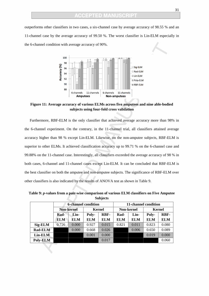
31

outperforms other classifiers in two cases, a six-channel case by average accuracy of 98.55 % and an

11-channel case by the average accuracy of 99.50 %. The worst classifier is Lin-ELM especially in

the 6-channel condition with average accuracy of 90%.

Figure 11: Average accuracy of various ELMs across five amputees and nine able-bodied subjects using four-fold cross validation

Furthermore, RBF-ELM is the only classifier that achieved average accuracy more than 98% in

the 6-channel experiment. On the contrary, in the 11-channel trial, all classifiers attained average

accuracy higher than 98 % except Lin-ELM. Likewise, on the non-amputee subjects, RBF-ELM is

superior to other ELMs. It achieved classification accuracy up to 99.71 % on the 6-channel case and

99.88% on the 11-channel case. Interestingly, all classifiers exceeded the average accuracy of 98 % in

both cases, 6-channel and 11-channel cases except Lin-ELM. It can be concluded that RBF-ELM is

the best classifier on both the amputee and non-amputee subjects. The significance of RBF-ELM over

other classifiers is also indicated by the results of ANOVA test as shown in Table 9.

Table 9: p-values from a pair-wise comparison of various ELM classifiers on Five Amputee Subjects

6-channel condition 11-channel condition Non-kernel Kernel Non-kernel Kernel

Rad-ELM

Lin-ELM

Poly-ELM

RBF-ELM

Rad-ELM

Lin-ELM

Poly-ELM

RBF-ELM

Sig-ELM 0.726 0.000 0.927 0.015 0.821 0.011 0.823 0.080 Rad-ELM

0.000 0.668 0.026

0.006 0.650 0.089 Lin-ELM 0.001 0.000 0.019 0.000 Poly-ELM

0.017

0.060

32

A one-way ANOVA test with a significance level set at p = 0.05 was applied to the amputee

subjects. Table 9 shows the results of ANOVA test for the amputee subjects. The result indicates that

when using six channels, the accuracy of RBF-ELM was significantly different from other ELM

classifiers (p = 0.015). However, in the 11-channel experiment, there was no significant difference in

the classification accuracy between RBF-ELM and other classifiers (p = 0.076) except Lin-ELM (p =

0.19e-3). Moreover, the ANOVA test on the non-amputee subjects (Table 10) highlights that RBF-

ELM was statistically superior to other ELM classifiers (p<0.001). In addition, Sig-ELM, Rad-ELM,

and Poly-ELM significantly obtained no different accuracy (p>0.05). In general, these facts confirm

the classification superiority of RBF-ELM over other ELM classifiers.

Table 10: p-values from a pair-wise comparison of various ELM classifiers on Nine Able-bodied Subjects

6-channel condition 11-channel condition Non-kernel Kernel Non-kernel Kernel

Rad-ELM

Lin-ELM

Poly-ELM

RBF-ELM

Rad-ELM

Lin-ELM

Poly-ELM

RBF-ELM

Sig-ELM 0.902 0.000 0.673 0.000 0.857 0.000 0.073 0.018 Rad-ELM

0.000 0.570 0.000

0.000 0.067 0.024 Lin-ELM 0.000 0.000 1.000 0.206 0.000 Poly-ELM

0.000

0.206 1.000 0.024

Figure 12 shows the average classification accuracy of RBF-ELM on five amputee subjects in two

conditions: six channels and 11 channels. The recognition system using RBF-ELM was capable of

classifying the 12 finger movements by a minimum average accuracy of more than 97%. However,

the classifier underwent some difficulties in identifying signals from the amputee subjects, especially

for the subject A4. Based on the demographic data in Table 1, the subject A4 has been a hand

amputee for eight years. S/he might have a difficulty in imagining the intended finger movements due

to the length of time of the amputee condition. Meantime, the subject A1 and A3 who have been hand

amputees for four years performed well in imagining finger movements so that their signals were

more detectable than others.

33

Figure 12: Average classification accuracy of RBF-ELM on five-amputee subjects using four-cross validation

Different from Figure 12, Figure 13 presents the classification accuracy of RBF-ELM in

recognizing the intended classes of the five amputee subjects. The finger movements performed by

the amputees here are not the actual movements. They imagined the finger movements representing

12 finger movements aided by their healthy hands. The figure shows that RBF-ELM could classify all

classes correctly with average accuracies of more than 96% on the six-channel and 98% on the 11-

channel experiments. The easiest finger movement was the rest condition while little extension (Le)

and ring extension (Re) movements were the most difficult movements to identify. Furthermore,

middle extension (Me) and index extension (Ie) movements were the next two consecutive intricate

movements. Interestingly, most of the complicated movements were the extension movements, while

flexion movements were relatively easily recognized. To analyse the misclassified classes, we can

observe the confusion matrix plot presented in Figure 14. It seems that Le was identified as Re and

vice versa. Besides, Me was recognized as Le.

34

Figure 13: Average classification accuracy of RBF-ELM on 12 finger movement classes over five amputee subjects.

Figure 14: Average confusion matrix plot of six-channel RBF-ELM on five amputee subjects

As for the non-amputee subjects, the average accuracy of RBF-ELM on individual subjects is

depicted in Figure 15. RBF-ELM succeeded in recognizing 15 classes across nine subjects by the

average accuracy of more than 99 % in 6-channel and 11-channel cases. The most accurate

classification occurs in subject 4 in which the accuracy is comparatively the same, on 6-channel and

11-channel experiments. Obviously, 11-channel trials are more accurate than 6-channel trials.

35

Figure 15 Average classification accuracy of RBF-ELM on nine able-bodied subjects

Figure 16 Average classification accuracy of RBF-ELM on 15 finger motion over nine non-amputee subjects

In addition to the classification performances of subjects, we analyse the performance of finger

motions as well. On able-bodied subjects, depicted in Figure 16, the system can classify all classes by

the average accuracy of more than 99%. However, on the ring flexion (Rf), rest (R) and thumb

abduction (Ta), the accuracies are diverse and they descend to less than 99 % in the 6-channel case.

However, overall, RBF-ELM accurately recognizes 15 classes with the accuracy of more than 98 %.

To investigate misclassified classes, we plot the confusion matrix of the classification results, as

presented in Figure 17. Interestingly, the difference between the misclassified data is not clear

36

because the average errors are extremely small and relatively similar. Therefore, it confirms that RBF-

ELM’s performance clearly outperforms the other classifiers.

Figure 17 Average confusion matrix plot of six-channel RBF-ELM on nine non-amputee subjects

4.6.2 ELM and other classifiers

In this section, the performance of ELM is compared to other well-known classifiers to verify its

performance in recognizing finger motions over amputee and non-amputee subjects. In this work, we

compared ELM with some known classifiers such as SM-SVM, LS-SVM, LDA, and kNN. The

structure of the recognition system for these two subject groups is alike. In this comparison, ELM is

represented by RBF-ELM. The results are described in Figure 18.

The figure indicates that the accuracy of RBF-ELM has a higher value than the others in all

conditions. On six-channel amputee subjects, RBF-ELM was the most accurate classifier. It was far

superior to LDA and kNN, but it was slightly better than the SVM family, SM-SVM and LS-SVM.

Likewise, in the 11-channel case, RBF-ELM achieved the best accuracy, but the accuracy gap was not

as large as in the six-channel experiments.

37

Figure 18: Average accuracy comparison between RBF-ELM and other famous classifiers

Similar to the amputee subjects, the accuracy of RBF-ELM on the non-amputee subjects exceeded

that of other classifiers. Different from 6-channel amputee results, the average accuracies of 6-channel

trial on non-amputee subjects are close to each other except for LDA. On the other hand, the

accuracies are relatively the same for the 11-channel cases including LDA. It seems that the more

complex the data involved, the closer the accuracy of classifiers. The superiority of RBF-ELM is

more noticeable by considering the ANOVA test as presented in Table 11 and Table 12 which shows

p-values of ANOVA pair-wise test of various classifiers across five amputee subjects. It indicates that

on the amputee subjects, the accuracy of RBF-ELM was significantly different from LDA (p = 0.001)

but it was not significantly different to other rest classifiers (p = 0.436). Meanwhile, different results

occurred to the able-bodied subjects, as depicted in Table 12. In all cases, six-channel and 11-channel,

RBF-ELM attained accuracy, which was significantly different from the other classifiers (p = 0.001).

This fact means that RBF-ELM was clearly superior to the other classifiers in recognizing 15 finger

movement classes.

Table 11. p-values from a pair-wise comparison of different classifiers on five amputee subjects

6 channels 11 channels

SM-SVM LS-SVM LDA KNN SM-SVM LS-SVM LDA KNN

RBF-ELM 0.577 0.665 0.000 0.067 0.429 0.539 0.001 0.178

38

Table 12. p-values from a pair-wise comparison of different classifiers on nine non-amputee subjects

6 channels 11 channels

SM-SVM LS-SVM LDA KNN SM-SVM LS-SVM LDA KNN

RBF-ELM 0.000 0.000 0.000 0.000 0.000 0.000 0.000 0.008

The comparison of ELM and other familiar classifiers was undertaken not only in terms of

accuracy but also in the training time as shown in Table 13 and Table 14. For the amputee subjects,

the fastest training time was LDA followed by kNN. As for the ELM, the training time was far

quicker than the SVM family, SM-SVM, and LS-SVM, but slower than LDA and kNN. As for the

non-amputee subjects, because they have more data, their training time is slower. Interestingly, the

time difference between the kernel-based and node-based ELM is very noticeable in the non-amputee

cases. The kernel-based ELM consumed much more training time than the node-based ELM. This fact

confirms the benefit of the node ELM in which the calculation of output weight can be modified to

deal with extensive data (see Eq. (17).

Table 13. Training time of amputee subjects

Classifier Six-channel 11-channel

Mean (ms) Std Mean (ms) Std Sig-ELM 4.293 2.159 4.351 2.190 Rad-ELM 4.301 2.118 4.261 2.115 Lin-ELM 4.643 5.073 4.635 5.064 Poly-ELM 5.214 5.567 5.194 5.550 RBF-ELM 5.581 6.005 5.556 5.958 SM-SVM 66.402 88.639 54.973 69.084 LS-SVM 86.339 73.602 86.921 74.398

LDA 0.012 0.005 0.010 0.004 KNN 0.785 0.689 0.782 0.690

Table 14. Training time of non-amputee subjects Classifier Six-channel 11-channel

39


LDA 0.031 0.006 0.026 0.007 KNN 2.656 0.885 2.658 0.887

In addition to the training time, the testing time is presented as well, as shown in Table 15 and

Table 16. Table 15 indicates that the testing time of the kernel and non-kernel ELM is very close in

the amputee subjects. However, in the non-amputee subjects, the testing time of kernel-based ELM is

about double that of amputee subjects (Table 16). In comparison with SVM, the testing time of ELM's

family is far quicker than that of SVM's family in both the amputees and non-amputees. Overall, the

performance of ELM's family for finger classification is comparable to SVM's family in terms of

accuracy but superior to SVM's family in terms of the processing time. However, the processing time

of ELM is not comparable to those of LDA and kNN. LDA and kNN consumed much shorter time

than ELM’s family. Nevertheless, the processing time of ELM is still reasonable for the real-time

application.

Table 15. Testing time of amputee subjects

Classifier Six-channel 11-channel Mean (ms) Std Mean (ms) Std

Sig-ELM 1.493 0.088 1.530 0.105 Rad-ELM 1.500 0.097 1.505 0.085 Lin-ELM 1.387 0.944 1.183 0.960 Poly-ELM 1.559 1.014 1.341 1.038 RBF-ELM 1.668 1.094 1.435 1.112 SM-SVM 20.127 15.659 15.416 12.941 LS-SVM 26.907 10.802 24.825 11.671

LDA 0.004 0.001 0.004 0.001 KNN 0.243 0.107 0.220 0.112

40

Table 16. Testing time of non-amputee subjects

Classifier Six-channel 11-channel


LDA 0.006 0.001 0.005 0.001 KNN 0.473 0.088 0.473 0.088

4.6.3 Two-channel Experiment

The previous section presented the results of the proposed myoelectric recognition system on

amputee and able-bodied subjects using six and eleven channels. In this section, we investigate the

performance of the proposed system using two channels only. It is a challenge to develop a

recognition system that can handle less information from two EMG channels without compromising

the performance, as was the case in (Anam et al., 2013; Khushaba et al., 2012). The result is presented

in Table 17. Table 17 shows that RBF-ELM achieves the highest accuracy on both subjects with an

average accuracy of 92.73 % on amputee subjects and of 97.11 % on the able-bodied subjects.

Table 17. The average accuracy of two-channel experiments

Classifier Amputee Able-bodied

Mean (%) STD Mean (%) STD Sig-ELM 84.45 3.48 92.99 2.38

Radbas-ELM 85.40 3.14 93.12 2.31 Lin-ELM 68.35 2.83 79.08 5.35 Poly-ELM 83.36 3.65 93.21 2.05 RBF-ELM 92.73 2.07 97.11 0.97 SM-SVM 92.46 1.85 96.24 1.05 LS-SVM 92.50 1.92 96.34 1.04

LDA 75.00 3.74 87.77 3.44 kNN 87.91 2.94 94.63 1.73

41

4.6.4 Toward real-time implementation

All previous experiments were conducted using HPC. In fact, in real-time application, HPC may

not be used. Instead, an embedded system or an ordinary computer such as a desktop computer or

laptop will be utilized. Therefore, we investigate the performance of the system when it is working on

a laptop. In this experiment, a laptop computer with Intel Core i7 second generation with 4 GB RAM

will be used. In addition, the number of samples involved in the experiment was one-eighth of the

whole samples presented in Table 3 so as to be able to be processed in the laptop. The experimental

results are shown in Table 18.

Table 18 indicates that the accuracy of the M-PR using HPC on amputee is better than the one

using Laptop. The performance gaps are big enough (more than 2%) except for Lin-ELM, RBF-ELM,

LDA, and kNN with RBF-ELM is the most accurate classifier. Interestingly, on the able-bodied

subject, the classifiers running on Laptop performed better than those on HPC except Lin-ELM and

Poly-ELM. However, the performance difference is small, equal to or less than 1%. This result

indicates that the performance of RBF-ELM does not change much even when a low-performance

computer is used.

Table 18. The average accuracy of the 6-channel experiment using different computers

Classifier Amputee Able-bodied

Laptop HPC (HPC-Laptop) Laptop HPC (HPC-Laptop) Sig-ELM 80.09 95.94 15.85 99.42 98.81 -0.61

Radbas-ELM 83.16 96.29 13.13 99.40 98.84 -0.56 Lin-ELM 89.58 90.33 0.75 96.78 97.34 0.56 Poly-ELM 78.07 95.77 17.69 97.35 98.35 1.00 RBF-ELM 97.08 98.58 1.50 99.65 99.02 -0.63 SM-SVM 94.12 98.35 4.23 98.33 98.27 -0.06 LS-SVM 94.20 98.41 4.21 98.37 98.35 -0.02

LDA 91.98 92.04 0.06 98.80 98.03 -0.77 kNN 95.46 97.18 1.72 99.39 98.71 -0.68

It has been mentioned previously, Laptop employed one-eighth of the sample while HPC

processed all samples. This scenario should be taken because Laptop cannot handle a large number of

samples. Nevertheless, the training time of classifiers on Laptop is longer than those on HPC, such as

42

in Sig-ELM and Radbas-ELM. For the rest of classifiers, Laptop is quicker than HPC. As for the

testing time, the classifiers running on Laptop took less time than those on HPC.

Table 19. Training time of the 6-channel experiment on different computers

Classifier Amputee (ms) Able-bodied (ms) Laptop HPC Laptop HPC

Sig-ELM 13.83 4.29 35.22 7.338 Radbas-ELM 14.36 4.30 34.49 7.417

Lin-ELM 0.31 4.64 5.66 17.318 Poly-ELM 0.67 5.21 9.38 18.956 RBF-ELM 1.73 5.58 10.31 19.876 SM-SVM 4.35 66.40 18.16 324.064 LS-SVM 2.49 86.34 16.80 241.715

LDA 0.01 0.01 0.17 0.031 kNN 0.07 0.79 0.57 2.656

Table 20. Testing time of the 6-channel experiment on different computers

Classifier Amputee (ms) Able-bodied (ms) Laptop HPC Laptop HPC

Sig-ELM 0.12 1.49 0.35 1.35 Radbas-ELM 0.12 1.50 0.33 1.366

Lin-ELM 0.01 1.39 0.11 3.024 Poly-ELM 0.14 1.56 1.33 3.314 RBF-ELM 0.09 1.67 0.86 3.476 SM-SVM 0.38 20.13 4.55 54.275 LS-SVM 0.62 26.91 7.28 43.208

LDA 0.00 0.00 0.01 0.006 kNN 0.02 0.24 0.18 0.473

The EMG signal were collected in strict scenario to ensure that the collected signal is good and

reliable for the experiment. In fact, in real-time application, noises may corrupt the EMG signal.

Therefore, another experiment was performed to test the performance of computer dealing with

unwanted noises. In this experiment, white Gaussian noises with different signal-to-noise ratio

(SNRs) were added in the EMG signals. The classification processes were conducted in Laptop.

Figure 19 and Figure 20 describes the experimental results on able-bodied subjects and amputees,

respectively.

43

Figure 19. The average accuracy of classifiers with noised EMG signal on able-bodied subjects

Figure 19 shows that, on the able-bodied subject, the white Gaussian noises added in the original

EMG degrade the performance of the classifiers depending on SNR of the noises. All classifiers

attained the worst accuracy when SNR is lower than 10. Their performance is getting better when

SNR is more than 30. Another interesting finding is in regards to the performance of RBF-ELM. The

figure indicates the superiority of RBF-ELM over other classifiers across all SNRs tested. This trend

also occurs on the experiments involving the amputees. However, the accuracy is much lower than

those on the able-bodied subjects. For example, for SNR less than 10, RBF-ELM achieved an

accuracy of 76.24% and 43.12%, on able-bodied subjects and amputees, respectively. The influence

of noises in the signal obtained from amputees is very significant. It is known that the EMG collected

from amputees is not as good as the signal from the able-bodied subjects. The existence of noise

increases the complexity of the EMG signals. Therefore, the performance of classifiers is decreasing

when the decode the signal from amputee corrupted with noise. Overall, the experiments support the

results of all previous experiments that RBF-ELM consistently performx better than other tested

classifiers.

44

Figure 20. The average accuracy of classifiers with noised EMG signal on amputees

4.7 Discussion

This chapter aims to build an accurate and optimum pattern recognition system using different

variations of ELM for finger movement classification on amputees and non-amputees. To achieve

such a system, we investigated every part of the state-of-the-art of the pattern-recognition system.

Selecting the window length and window increment of the data segmentation started the finding of the

optimal system. We found that a 200-ms window length and a 25-ms window increment were the

optimum choices for the pattern-recognition system which comply with the optimal time delay

suggested by Farrell and Weir (2007). These segmentation parameters enabled us to create a pattern-

recognition system, which is ready for real-time application.

In the feature extraction method, this work introduced a new feature set. The proposed feature set

mainly comprises Hargrove’s features plus SS (sample skewness) and HTD (Hjorth time domain)

parameters (see section 4.3). This additional feature set was able to provide more informative features

for the classifier. The classification accuracy of the new feature set was higher than Hargrove’s

features, especially for the amputee subjects (Table 5).

As for the dimensionality reduction method, the results supported the claim of Cai et al. (2008)

and our published work (Anam et al., 2013) that SRDA is faster than LDA. LDA took more time in

45

reducing the dimension of 6-channel features than SRDA, but the time difference between the two is

not significant (p > 0.05). However, the processing time of LDA is much longer than that of SRDA

when reducing the dimension of 11-channel features (p < 0.05). As for OFNDA (Khushaba et al.,

2010), its reduction time is large enough, and it is not comparable to SRDA or even LDA. The

processing time of OFNDA is long because OFNDA consists of two stages: principal components

analysis (PCA) and fuzzy discriminant analysis (FNDA). PCA in OFNDA is needed to overcome the

singularity problem in FNDA.

Unlike the processing time, the accuracy of the system using SRDA is similar to LDA and

OFNDA (p > 0.05). Probably, this finding can be used to make a comment on the outcomes of Al-

Timemy et al.’s work (Al-Timemy et al., 2013). Their work, which employed the same data as used in

this chapter, utilized OFNDA as a dimensionality reduction and LDA as a classifier. As a note, LDA

can be used as either a dimensionality reduction or a classifier. On the six-channel experiment,

OFNDA+LDA was able to achieve a high accuracy of about 98 % on the able-bodied subjects, but it

showed a lower accuracy on the amputee subjects with the accuracy of about 90%. Comparing their

results and the results in this paper, the proposed recognition system, which utilizes SRDA+ELM,

attained the accuracy of approximately 99% on the able-bodied subjects and around 98% on the

amputee subjects. Because OFNDA and SRDA have similar performances in term of accuracy, the

inaccuracy of Al-Timemy et al.’s work on the amputee subjects was probably caused by LDA as a

classifier. This assumption is supported by the results in Figure 18, which informs the shortcoming of

LDA as a classifier.

The utilization of SRDA as a dimensionality reduction method is important in constructing a

recognition system that is powerful and fast. We have shown that SRDA is equivalent to other LDA

variances, but it is superior to others in term of speed. SRDA should be better than another well-

known methods of dimensionality reduction such as PCA. Martínez and Kak (2001) proved that LDA

outperform PCA especially for large data as we used in this work.

46

Finally, we discuss the classifier’s performances. The experimental results confirm that the ELM

(extreme learning machine) was capable of classifying the EMG signal of the non-amputee and

amputee subjects. Among the different types of ELM, the kernel-based ELM with RBF kernel

outperformed other types of ELM. This finding supports the results of Huang et al. (2012) that, on

some cases, RBF-ELM achieved better accuracy than the node-based ELM: sigmoid-additive node

(Sig-ELM) and the radial basis node ELM (Rad-ELM). However, we found that the kernel-based

ELM needs more processing time than the non-kernel-based ELM, especially on the large data as

shown in Table 13 and Table 14.

The large data problem on the node-based ELM has been solved by Huang et al. (2012) but it is

still unsolved on the kernel-based ELM. They had manipulated the output of node-based ELM (see

Eq. (17) in section 2.2) in such a way that the dimension of a feature-mapping matrix has L x L order,

instead of N x N as in the kernel-based ELM (see Eq. (24) in section 2.3). L is the number of hidden

nodes, and N is the training data number. In fact, for a large feature, the number L is far smaller than

N. As a result, the training time of the node-based ELM is faster than the kernel-based ELM because

the node-based ELM deals with L x L order instead of N x N order.

The comparison of the ELM, which is represented by RBF-ELM, and with other well-known

classifiers, confirms that the ELM is comparable with the well-known SVM even though there is no

iterative learning on the ELM’s weight. The superiority of the ELM over the SVM is more

noteworthy if the processing time of the classifiers is considered. It is true that the ELM was not the

fastest classifier tested in this work. LDA was the fastest one, yet LDA was the least accurate

classifier. kNN was faster than the ELM, but its performance was still under that of the ELM

especially RBF-ELM. In addition, the fact that the ELM is far superior to LDA especially with small

channel numbers disproves the statement of (Hargrove, Scheme, Englehart, & Hudgins, 2010) on the

classification process. They stated that classification is a trivial process as long as the feature set and

the dimensionality reduction are chosen properly.

47

Furthermore, in dealing with small channel numbers, which is two channels, the RBF-ELM and

SVM family performed better than other classifiers. Even though the RBF-ELM achieved better

accuracy, the one-way ANOVA test on the accuracy across all subjects shows that the difference was

not significant (p>0.05; see Table 11 and Table 12). Using RBF-ELM, the recognition system attained

accuracy of about 97% on nine non-amputee subjects and roughly 92% on the five amputee subjects.

Compared to the work of Khushaba et al. (2012) which achieved around 92% accuracy on eight able-

bodied subjects, the proposed recognition system attained better accuracy on the able-bodied subjects

(97%). Actually, Khushaba et al. (2012) utilized the SVM but their accuracy was much less accurate

than what was reported here. It seems that Khushaba et al.’s system did not optimize the parameters

of SVM. In fact, parameter optimization is a crucial aspect in SVM classification (Huang et al., 2012).

The proposed recognition using ELM especially RBF-ELM have shown effective and powerful for

finger movement recognition. The proposed system will not be useful unless it is implemented in real-

time application. To anticipate some issues in real-time application, we tested the proposed system on

different scenarios. The first scenario is to run the proposed system in a low-performance computer

using a laptop. The experimental results in Table 18 show that the system with RBF-ELM has the

most stable performance for amputee and non-amputees among other tested classifiers. The second

scenario is to test the proposed system with EMG signals corrupted with white Gaussian noise. The

existence of noise with SNR less than 10 downgrades the performance of the classifiers significantly

on both, amputees and non-amputees. Again, RBF-ELM shows its superiority over other tested

classifiers, as shown in Figure 19 and Figure 20. The system with RBF-ELM attained the highest

accuracy on both subjects and across all SNR values. Another consideration that should be addressed

when preparing for real-time classification is features.

This work proposed a feature set consisting of 16 features per channel. This number may be

overload for an embedded system or a low-performance computer. We have investigated the

performance of the proposed approach when the number of features is reduced, as shown in Table 5.

Table 5 reveals that the proposed feature set could achieve an accuracy of around 93% and 97% on

48

amputees and non-amputees, respectively. Interestingly, the proposed recognition system can still

attain a good accuracy, i.e., more than 90% when using 4 features or 5 features of the Englehart’s and

Hudgin’s sets, respectively. As a note, Englehart’s and Hudgin’s set are composed of time domain

features. However, the performance of the proposed system decreased when using Hjorth (3 features)

and autoregressive (6 features) coefficient parameters. It means, the proposed approach work well on

the time domain feature even though the number of features is reduced. Therefore, it is possible to

implement the proposed system in the embedded system or the low-performance computer using a

small number of time domain features.

To evaluate the proposed system, we provide some works related to the finger movement

identification, as presented in Table 21. The table does not indicate that the system developed here is

the best one because the situation, experimental setup and other considerations may be different

application to application. However, it can be used to measure the performance of the proposed

system. Overall, this work exhibited the most accurate system. In addition, it was the most stable

system because accuracy was still high even though only two channels were used. Another interesting

finding is that the accuracy gap of the non-amputee and amputee subjects was not very large. In the

six-channel experiments, the accuracy difference of RBF-ELM on the amputee subjects and non-

amputee subjects was 0.95%.

Table 21. Comparison of Various Research on Finger Movement Recognition Work Nch Finger Class Accuracy (%) Subjects Mode

Tenore et al. (2009)

19 10 Id & 2 Cm 93.4 5 H 1 A OF 19 10 Id & 2 Cm 87.80 1 A OF 19 10 Id 92.83 1 A OF

Cipriani et al. (2011)

8 7 Id & 1 Cm 89.00 5 H OL 8 7 Id & 1 Cm 79.00 5A OL

Khushaba et al. (2012)

2 5 Id & 5 Cm 92.00 8 H OF 2 5 Id & 5 Cm 90.00 8H OL

Al-Timemy et al. (2013)

6 12 Id & 3 Cm 98.55 10 H OF 6 12 Id 90.57 6 A OF

This work 6 12 Id & 3 Cm 99.50 9H OF

49

6 12 Id 98.55 5A OF 2 12 Id & 3 Cm 97.11 9H OF 2 12 Id 92.73 5A OF

Nch = Number of channels, Id = Individual finger movements, Cm = Combined Finger movements, H = Healthy Subjects, A = Amputees, OF= Offline classification, OL = Online Classification

5. Conclusion

All components in this recognition system were determined using experimental procedures. As a

result, a powerful classification system that can work well on able-bodied and amputee subjects had

been achieved. However, this work only studies the offline classification system. In fact, the system

was designed to be ready for real-time application. The system recognition produced here fulfils three

conditions for a real-time recognition system (Englehart & Hudgins, 2003). Its performance was

highly accurate; it was able to detect the user’s intention with accuracy of roughly 99% on the able-

bodied subjects and around 98% on the trans-radial amputees. In addition, it has easy interface for

direct control so that it relieves the user’s mental difficulties in wearing the hand rehabilitation device.

Finally, it meets the optimal delay time for a real application in the range 100–125 ms.

Different ELM classifiers have been tested in this work. This work presents, on average, the

kernel-based ELM is better than the node-based ELM. An attempt to enhance the performance of the

node-based ELM should be carried out. One weakness of the node-based ELM is that the input weight

was determined arbitrarily and free from the training data so that the ELM produced is not optimum

for a specific case. Therefore, optimization of the node-based ELM should be undertaken.

Developments, such as the evolutionary extreme learning machine (E-ELM) (Zhu et al., 2005) and the

dynamic extreme learning (D-ELM) (Zhang, Lan, Huang, Xu, & Soh, 2013) can be implemented for

finger movement classification.

In summary, this paper presented the detailed investigation of the implementation of different

types of ELM for the myoelectric pattern recognition system. The experiment results in a recognition

system, which is fast, accurate, and easy to develop to classify 15 and 12 finger movements on nine

able-bodied subjects and five amputee subjects, respectively. The proposed system introduced a new

feature set comprising MAVS, ZC, SSC, SS, WL, RMS, AR6, and HTD forming 16 features per

50

channel. The EMG signal is segmented using a 200-ms sliding window with a 25-ms shift. The

extracted features are concatenated to yield a large feature. The combined feature dimension is

reduced using SRDA, a swift version of LDA. Then the reduced features are fed to the ELM to be

identified and classified into the intended class. By using the best ELM classifier, RBF-ELM, the

pattern recognition system achieved accuracy of 98.55% on the amputee subjects and 99.5% on the

able-bodied subjects using six EMG channels. Meanwhile, using two EMG channels, it achieved

accuracy of 97.11% and 92.73% on the non-amputees and amputees respectively. In term of accuracy,

the ELM family is comparable to the most well-known classifier, the SVM family. However, in terms

of the processing time, the ELM family is superior to the SVM family.

Acknowledgment

The main author would like to thank the Directorate of Higher Education, the Republic of Indonesia

for their financial support. In addition, the authors very much appreciate the kindness of Dr. Ali H Al-

Timemy (Al-Timemy et al., 2013) for his generosity in sharing the data.

References

Al-Timemy, A. H., Bugmann, G., Escudero, J., & Outram, N. (2013). Classification of Finger Movements for the Dexterous Hand Prosthesis Control With Surface Electromyography. IEEE Journal of Biomedical and Health Informatics, 17, 608-618.

Anam, K., & Al-Jumaily, A. (2015). A novel extreme learning machine for dimensionality reduction on finger movement classification using sEMG. In The 7th International IEEE/EMBS Conference on Neural Engineering (NER) (pp. 824-827). Montpellier, France.

Anam, K., Khushaba, R., & Al-Jumaily, A. (2013). Two-channel surface electromyography for individual and combined finger movements. In Proceeding of the 35th Annual International IEEE Engineering Medicine and Biology Society Conference (EMBC) (pp. 4961-4964).

BenoíT, F., Van Heeswijk, M., Miche, Y., Verleysen, M., & Lendasse, A. (2013). Feature selection for nonlinear models with extreme learning machines. Neurocomputing, 102, 111-124.

Cai, D., He, X., & Han, J. (2008). SRDA: An efficient algorithm for large-scale discriminant analysis. IEEE Transactions on Knowledge and Data Engineering, 20, 1-12.

Cao, J., Lin, Z., & Huang, G.-B. (2012). Self-adaptive evolutionary extreme learning machine. Neural processing letters, 36, 285-305.

51

Chan, A. D. C., & Green, G. C. (2007). Myoelectric control development toolbox. In Proceeding of the 30th Conference of Canadian Medical and Biological Engineering Society (CMBES) (pp. M0100-0101).

Chang, C.-C., & Lin, C.-J. (2011). LIBSVM: a library for support vector machines. ACM Transaction on Intelligent System and Techology (TIST), 2, 27.

Chen, Z. X., Zhu, H. Y., & Wang, Y. G. (2013). A modified extreme learning machine with sigmoidal activation functions. Neural Computing and Applications, 22, 541-550.

Cipriani, C., Antfolk, C., Controzzi, M., Lundborg, G., Rosen, B., Carrozza, M. C., & Sebelius, F. (2011). Online Myoelectric Control of a Dexterous Hand Prosthesis by Transradial Amputees. IEEE Transactions on Neural Systems and Rehabilitation Engineering, 19, 260-270.

Deng, W.-Y., Zheng, Q.-H., & Wang, Z.-M. (2014). Cross-person activity recognition using reduced kernel extreme learning machine. Neural networks, 53, 1-7.

Englehart, K., Hudgin, B., & Parker, P. A. (2001). A wavelet-based continuous classification scheme for multifunction myoelectric control. IEEE Transactions on Biomedical Engineering, 48, 302-311.

Englehart, K., & Hudgins, B. (2003). A robust, real-time control scheme for multifunction myoelectric control. IEEE Transactions on Biomedical Engineering, 50, 848-854.

Farrell, T., & Weir, R. F. (2008). Analysis window induced controller delay for multifunctional prostheses. In Proceeding of MyoElectric Controls/Powered Prosthetics Symposium: Myoelectric Symposium.

Farrell, T. R., & Weir, R. F. (2007). The optimal controller delay for myoelectric prostheses. IEEE Transactions on Neural Systems and Rehabilation Engineering, 15, 111-118.

Fletcher, R. (2013). Practical methods of optimization: John Wiley & Sons.

Fukunaga, K. (2013). Introduction to statistical pattern recognition: Academic press.

Hargrove, L. J., Englehart, K., & Hudgins, B. (2007). A comparison of surface and intramuscular myoelectric signal classification. IEEE Transactions on Biomedical Engineering, 54, 847-853.

Hargrove, L. J., Scheme, E. J., Englehart, K. B., & Hudgins, B. S. (2010). Multiple Binary Classifications via Linear Discriminant Analysis for Improved Controllability of a Powered Prosthesis. IEEE Transactions on Neural Systems and Rehabilation Engineering, 18, 49-57.

Huang, G., Huang, G.-B., Song, S., & You, K. (2015). Trends in extreme learning machines: A review. Neural networks, 61, 32-48.

Huang, G., Song, S., Gupta, J. N., & Wu, C. (2014). Semi-supervised and unsupervised extreme learning machines. IEEE Transactions on Cybernetics, 44, 2405-2417.

52

Huang, G.-B., Chen, L., & Siew, C. K. (2006). Universal approximation using incremental constructive feedforward networks with random hidden nodes. IEEE Transactions on Neural Networks, 17, 879-892.

Huang, G.-B., Li, M.-B., Chen, L., & Siew, C.-K. (2008). Incremental extreme learning machine with fully complex hidden nodes. Neurocomputing, 71, 576-583.

Huang, G.-B., Zhu, Q.-Y., & Siew, C.-K. (2006). Extreme learning machine: Theory and applications. Neurocomputing, 70, 489-501.

Huang, G. B., Zhou, H., Ding, X., & Zhang, R. (2012). Extreme learning machine for regression and multiclass classification. IEEE Transactions on Systems, Man, and Cybernetics, Part B (Cybernetics), 42, 513-529.

Hudgins, B., Parker, P., & Scott, R. N. (1993). A new strategy for multifunction myoelectric control. IEEE Transactions on Biomedical Engineering, 40, 82-94.

Iosifidis, A., Tefas, A., & Pitas, I. (2013). Dynamic action recognition based on dynemes and Extreme Learning Machine. Pattern Recognition Letters, 34, 1890-1898.

Khushaba, Kodagoda, S., Takruri, M., & Dissanayake, G. (2012). Toward improved control of prosthetic fingers using surface electromyogram (EMG) signals. Expert Systems with Applications, 39, 10731-10738.

Khushaba, R. N., Al-Ani, A., & Al-Jumaily, A. (2010). Orthogonal Fuzzy Neighborhood Discriminant Analysis for Multifunction Myoelectric Hand Control. IEEE Transactions on Biomedical Engineering, 57, 1410-1419.

Lee, H., Kim, S.-J., Kim, K., Park, M. S., Kim, S.-K., Parfk, J. H., & Oh, S.-R. (2011). Online remote control of a robotic hand configurations using sEMG signals on a forearm. In The IEEE International Conference on Robotics and Biomimetics (ROBIO) (pp. 2243-2244).

Li, G., Schultz, A. E., & Kuiken, T. A. (2010). Quantifying pattern recognition—Based myoelectric control of multifunctional transradial prostheses. IEEE Transactions Neural Systems and Rehabilation Engineering, 18, 185-192.

Liu, H., Yu, L., Wang, W., & Sun, F. (2016). Extreme learning machine for time sequence classification. Neurocomputing, 174, 322-330.

Martínez, A. M., & Kak, A. C. (2001). Pca versus lda. IEEE Transactions on Pattern Analysis and Machine Intelligence, 23, 228-233.

Mohammed, A. A., Minhas, R., Wu, Q. J., & Sid-Ahmed, M. A. (2011). Human face recognition based on multidimensional PCA and extreme learning machine. Pattern recognition, 44, 2588-2597.

Oskoei, M. A., & Hu, H. (2007). Myoelectric control systems—A survey. Biomedical Signal Processing and Control, 2, 275-294.

53

Oskoei, M. A., & Hu, H. (2008). Support Vector Machine-Based Classification Scheme for Myoelectric Control Applied to Upper Limb. IEEE Transactions on Biomedical Engineering, 55, 1956-1965.

Pao, Y.-H., Park, G.-H., & Sobajic, D. J. (1994). Learning and generalization characteristics of the random vector functional-link net. Neurocomputing, 6, 163-180.

Pao, Y.-H., & Takefuji, Y. (1992). Functional-link net computing. IEEE Computer Journal, 25, 76-79.

Park, M. S., Kim, K., & Oh, S. R. (2011). A fast classification system for decoding of human hand configurations using multi-channel sEMG signals. In IEEE International Workshop on Intelligent Robots and Systems (IROS) (pp. 4483-4487).

Rong, H.-J., Ong, Y.-S., Tan, A.-H., & Zhu, Z. (2008). A fast pruned-extreme learning machine for classification problem. Neurocomputing, 72, 359-366.

Scheme, E., & Englehart, K. (2011). Electromyogram pattern recognition for control of powered upper-limb prostheses: State of the art and challenges for clinical use. Journal of rehabilitation research and development, 48, 643.

Schlogl, A., & Brunner, C. (2008). BioSig: a free and open source software library for BCI research. Computer, 41, 44-50.

Shi, J., Cai, Y., Zhu, J., Zhong, J., & Wang, F. (2013). SEMG-based hand motion recognition using cumulative residual entropy and extreme learning machine. Medical & Biological Engineering & Computing, 51, 417-427.

Smith, L. H., Hargrove, L. J., Lock, B. A., & Kuiken, T. A. (2011). Determining the optimal window length for pattern recognition-based myoelectric control: balancing the competing effects of classification error and controller delay. IEEE Transactions on Neural Systems and Rehabilation Engineering, 19, 186-192.

Tenore, F. V. G., Ramos, A., Fahmy, A., Acharya, S., Etienne-Cummings, R., & Thakor, N. V. (2009). Decoding of individuated finger movements using surface electromyography. IEEE Transactions on Biomedical Engineering, 56, 1427-1434.

Teo, T., Logenthiran, T., & Woo, W. (2015). Forecasting of photovoltaic power using extreme learning machine. In Smart Grid Technologies-Asia (ISGT ASIA), 2015 IEEE Innovative (pp. 1-6).

Tkach, D., Huang, H., & Kuiken, T. A. (2010). Study of stability of time-domain features for electromyographic pattern recognition. IEEE Transaction on Neural Systems and Rehabilitation Engineering, 7, 21.

TouchBionics. (2007). The Big Picture: Bionic Hand. Spectrum, IEEE, 44, 22-22.

Tsenov, G., Zeghbib, A. H., Palis, F., Shoylev, N., & Mladenov, V. (2006). Neural Networks for Online Classification of Hand and Finger Movements Using Surface EMG signals. In The 8th Seminar on Neural Network Application in Electrical Engineering (NEUREL) (pp. 167-171).

54

Uchida, N., Hiraiwa, A., Sonehara, N., & Shimohara, K. (1992). EMG pattern recognition by neural networks for multi fingers control. In The 14th Annual International Conference of IEEE EMBS (Vol. 3, pp. 1016-1018): IEEE.

Wang, G., Zhao, Y., & Wang, D. (2008). A protein secondary structure prediction framework based on the extreme learning machine. Neurocomputing, 72, 262-268.

Wang, Y., Cao, F., & Yuan, Y. (2011). A study on effectiveness of extreme learning machine. Neurocomputing, 74, 2483-2490.

Wong, P. K., Wong, K. I., Vong, C. M., & Cheung, C. S. (2015). Modeling and optimization of biodiesel engine performance using kernel-based extreme learning machine and cuckoo search. Renewable Energy, 74, 640-647.

Xu, Y., & Shu, Y. (2006). Evolutionary extreme learning machine–based on particle swarm optimization. In Advances in Neural Networks-ISNN 2006 (pp. 644-652): Springer.

Zhang, R., Lan, Y., Huang, G.-b., & Xu, Z.-B. (2012). Universal approximation of extreme learning machine with adaptive growth of hidden nodes. IEEE Transactions on Neural Networks and Learning Systems, 23, 365-371.

Zhang, R., Lan, Y., Huang, G.-B., Xu, Z.-B., & Soh, Y. C. (2013). Dynamic Extreme Learning Machine and Its Approximation Capability. IEEE Transactions on Cybernetics, 43, 2054-2065.

Zhu, Q.-Y., Qin, A. K., Suganthan, P. N., & Huang, G.-B. (2005). Evolutionary extreme learning machine. Pattern recognition, 38, 1759-1763.

Zong, W., & Huang, G.-B. (2011). Face recognition based on extreme learning machine. Neurocomputing, 74, 2541-2551.

Zong, W., Zhou, H., Huang, G.-B., & Lin, Z. (2011). Face recognition based on kernelized extreme learning machine. In Autonomous and Intelligent Systems (pp. 263-272): Springer.

Evaluation of extreme learning machine for classification...

Documents

Transcript of Evaluation of extreme learning machine for classification...