Evaluation of Enhanced Recharge Potential to the …€¦ · 2-4 Mean annual and monthly...

Report 355 by Bridget Scanlon, Edward S. Angle, Brent Christian, Jonathan Pi, Kris Martinez, Robert Reedy, Radu Boghici, and Rima Petrossian

Texas Water Development Board P.O. Box 13231, Capitol Station Austin, Texas 78711-3231

August 2003

Texas Water Development Board

Report 355

Evaluation of Enhanced Recharge Potential to the Ogallala Aquifer in the Brazos River Basin, Hale County, Texas

by Bridget Scanlon1 Edward S. Angle Brent Christian Jonathan Pi Kris Martinez Robert Reedy1 Radu Boghici Rima Petrossian

1-The University of Texas at Austin, Bureau of Economic Geology

August 2003

This page intentionally blank.

ii

Texas Water Development Board

E. G. Rod Pittman, Chairman, Lufkin Thomas Weir Labatt III, Member, San Antonio

Jack Hunt, Vice Chairman, Houston Wales H. Madden, Member, Amarillo

Dario Vidal Guerra, Jr., Member, Edinburg William W. Meadows, Member, Fort Worth

J. Kevin Ward, Executive Administrator

Authorization for use or reproduction of any original material contained in this publication, i.e., not obtained from other sources, is freely granted. The Board would appreciate acknowledgment. The use of brand names in this publication does not indicate an endorsement by the Texas Water Development Board or the State of Texas.

Published and distributed by the

Texas Water Development Board P.O. Box 13231, Capitol Station

Austin, Texas 78711-3231

August 2003 Report 355

(Printed on recycled paper)

iii

This page intentionally blank.

iv

Table of Contents 1.0 Executive Summary ............................................................................................................ 1 1.1 Recommendations for Future Work........................................................................ 2 2.0 Introduction ......................................................................................................................... 2 2.1 Previous Work......................................................................................................... 4 2.2.1 Natural Recharge......................................................................................... 4 2.1.2 Enhanced Recharge ..................................................................................... 7 2.2 Site Description ....................................................................................................... 8 3.0 Methods............................................................................................................................. 12 3.1 Surface-Water Modeling ....................................................................................... 12 3.2 EM Induction......................................................................................................... 17 3.3 Soil Texture, Water Content, and Chloride........................................................... 20 3.4 Hydraulic Conductivity ......................................................................................... 20 3.4.1 Reservoir Infiltration ................................................................................. 20 3.4.2 Ring Infiltrometer Tests ............................................................................ 22 3.4.3 Guelph Permeameter Tests........................................................................ 22 4.0 Results ............................................................................................................................... 23 4.1 Surface-Water Model Simulations ........................................................................ 23 4.2 EM Induction......................................................................................................... 25 4.3 Soil Texture and Water Content............................................................................ 25 4.4 Chloride Tracer ..................................................................................................... 30 4.5 Reservoir Infiltration ............................................................................................. 30 4.6 Hydraulic Conductivity ......................................................................................... 30 5.0 Discussion ......................................................................................................................... 38 6.0 Recommendations ............................................................................................................. 38 7.0 Conclusions ....................................................................................................................... 39 8.0 Acknowledgments............................................................................................................. 40 9.0 References ......................................................................................................................... 41

List of Figures 2-1 Location of SCS reservoirs in the Southern High Plains .................................................... 3 2-2 Location of study area that includes SCS reservoirs........................................................... 9 2-3 The catchment for Running Water Draw upstream of the Plainview gauging station........ 9 2-4 Mean annual and monthly precipitation measured at the Hart weather station

from 1955 to 1979 ............................................................................................................. 10 2-5 Location of playa lakes in the study area .......................................................................... 11 3-1 Topography of the catchment based on 1:250,000 DEM.................................................. 14 3-2 Soil cover data for the study area based on STATSGO.................................................... 15 3-3 Spatial variability in land cover in the study area ............................................................. 15 3-4 Location of weather stations in the study area .................................................................. 16 3-5 Location of EM transects, boreholes (Giddings, Mobile), Guelph permeameter tests

and ring infiltrometer tests in SCS 3 reservoir.................................................................. 18 3-6 Location of EM transects, boreholes (Giddings, Mobile), and ring infiltrometer tests in SCS 4 reservoir ............................................................................................................. 19 4-1 Simulated and measured mean annual stream flow at Plainview, Texas.......................... 24

v

4-2 Apparent electrical conductivity measured with the EM 31 meter in the vertical and horizontal dipole mode in representative transects in SCS 3 ........................................... 26

4-3 Apparent electrical conductivity measured with the EM 31 meter in the vertical and horizontal dipole mode in representative transects in SCS 4 ............................................ 28

4-4 Profiles of soil texture, gravimetric water content, and chloride for boreholes in SCS 3 reservoir.................................................................................................................. 29

4-5 Profiles of soil texture, gravimetric water content, and chloride for boreholes in SCS 4 reservoir.................................................................................................................. 32

4-6 Variations in water levels in SCS 4 reservoir from March through September 2000 and corresponding precipitation.......................................................................................... 34

List of Tables 2-1 Published recharge values, Southern High Plains............................................................... 5 2-2 Areas, capacities, release rates, and conductivity data for SCS 3 and SCS 4 reservoirs .. 10 2-3 Playa statistics for the study area ...................................................................................... 11 3-1 Water balance results for the different densities of hydrologic response units................. 16 3-2 Characteristics of electromagnetic induction conductivity meters ................................... 18 3-3 Summary of boreholes drilled, date drilled, analyses conducted on soil samples,

and tests conducted............................................................................................................ 21 4-1 Simulated flows to SCS 3 reservoir .................................................................................. 24 4-2 Mean apparent electrical conductivity for EM transects in SCS 3 and SCS 4

reservoirs ........................................................................................................................... 27 4-3 Borehole number; mean percentage values of sand, silt, and clay; carbonate

content range and mean water content, and mean and maximum chloride concentration for SCS 3 and SCS 4 reservoirs.................................................................. 31

4-4 Results of ring infiltrometer tests ...................................................................................... 35 4-5 Field saturated hydraulic conductivity results based on Guelph permeameter

measurements .................................................................................................................... 36

Appendix I Borehole number, sand, silt, clay percentages, textural classification, gravimetric water

content, chloride content in soil samples, and chloride concentrations in pore water. ....... 49

Appendix II Summary of Running Water Draw reservoirs................................................................... 65

vi

1.0 Executive Summary

Preserving, conserving, and optimizing the use of groundwater from the Ogallala aquifer are critical issues for the Southern High Plains because of continuing demands on groundwater coupled with decreasing groundwater supplies. This study evaluates groundwater recharge from Soil Conservation Service (SCS) (currently the Natural Resources Conservation Service) reservoirs to determine whether recharge could be enhanced by increasing storage capacity or by modifying the bottom of the reservoirs.

This technical evaluation includes results of surface-water modeling and field studies on two of the six reservoirs in Running Water Draw in Hale County, Texas. These reservoirs were built in 1976 and 1982 by the SCS for flood control. Under current regulations (Sec. 11.142, Texas Water Code), reservoirs cannot store more than an average of 200 acre-feet of water over a 12-month period, unless a permit is obtained from the Texas Commission on Environmental Quality (TCEQ).

The SCS 3 reservoir was dry throughout the study period (March 1999-October 2000). Surface-water modeling, based on data from 1950 to 1978, shows SCS 3 held runoff ranging from 1 acre-foot in 1976 to 9,380 acre-feet in 1950. These data indicate that the reservoirs could store much more water during periods of above-normal precipitation. Under current regulations, a maximum of 1,200 acre-feet from all six reservoirs is available for storage. Currently two of the six SCS reservoirs in Running Water Draw have obtained permits and installed plugs to increase storage capacity from 200 acre-feet per reservoir to 424 and 4,427 acre-feet (4,851 acre-feet total). If the area experienced a flood similar to the one in 1941, 24,569 acre-feet of surface water would be available for storage and recharge. If the highest recorded annual rainfall (1941) were to occur again, 31,353 acre-feet of surface water would be available for storage and recharge.

Inflows from precipitation and irrigation return flows into the SCS 4 reservoir resulted in about 155 acre-feet of ponded water during a 6-month period (March-September 2000) during the study. Approximately 35 percent of this water evaporated, whereas the remaining 65 percent infiltrated. Some of the infiltrated water eventually evaporated from the soil. The rest will ultimately recharge the Ogallala aquifer. Assuming the average reservoir capacity is 1,985 acre-feet and all reservoirs in Running Water Draw had the same infiltration rate as SCS 4 (65 percent) and the current storage limitations were eliminated from the other four SCS reservoirs, the potential infiltration from a 50- to 100-year flood event would be approximately 7,742 acre-feet for all six reservoirs. Actual recharge would depend on the evaporation rate of the water in storage.

SCS 3 and SCS 4 have fine-grained sediments in the upper 1 to 3 ft of the reservoirs and coarser sediments at greater depths. Previous studies conducted on playas indicate removing surficial fine-grained sediments could increase recharge by 10 times. Modifying fine-grained sediments in the SCS reservoirs may also increase recharge. Modifying SCS reservoirs would impact local recharge; however, it would not enhance recharge throughout the region.

Senate Bill 1, enacted by the 75th Legislature, requires Regional Water Planning Groups (RWPGs) to determine the economic impact of being unable to meet future water needs. The

1

Llano Estacado RWPG has determined that the region would lose approximately $340 of output and $68 of income per acre-foot of irrigation water that is not available. A conservative estimate of the cost of obtaining permits for the four SCS reservoirs is $20,000. This estimate is based on TCEQ’s maximum fee of $5,000 per permit. Modifying surface sediments to enhance recharge on a flood-event basis is estimated to cost $18,000, or $3,000 per SCS reservoir. Together the total cost of potentially enhancing recharge from 3,673 to 7,742 acre-feet during a 50- to 100-year flood event would be $38,000, or $9.34 per acre-foot. The cost-benefit analysis of installing plugs in the four remaining SCS structures in the Running Water Draw and modifying surface sediments in all six would be positive, especially if considered on a local basis.

1.1 Recommendations for Future Work

Additional studies would be required to assess the feasibility of enhancing recharge by modifying soil profiles in SCS reservoirs. Additional surface-water modeling would also be required to quantify runoff from surface-water drainages, such as Running Water Draw, and to help determine the impact of efforts to enhance recharge on downstream surface-water rights. Specifically, additional studies would remove fine-grained sediments in selected reservoirs and increase storage capacity. Detailed monitoring would be conducted to quantify recharge. General statistics and surface-water characteristics would be assessed for all 62 reservoirs in the Southern High Plains, and the net impact on recharge would be evaluated.

This study focused on drainages. While surface-water bodies drain approximately 10 percent of the surface area of the Southern High Plains, playas drain the remaining 90 percent. Previous studies indicate that removing fine-grained sediments from the bottom of playas further enhance recharge. Enhancing recharge in playas could impact recharge to the aquifer to a much greater extent than altering SCS reservoirs could. As such, any future studies should also include playas. Future studies could include a classification of playas based on Landsat imagery, including color IR photography.

Recharge enhancement would probably focus on playas whose ponding times fall into a midrange that has been based on the length of ponding. About 30 to 50 playas could be identified for recharge enhancements, resulting in about 1 to 2 playas per county. If possible, duplicate playas that have similar characteristics could be identified. Recharge enhancement could be conducted at one of the two playas, and the effectiveness of enhancing recharge could be quantified by comparing the results with the recharge evaluation from the control playa. Recharge could be enhanced by the targeted removal of surficial fine-grained sediments. If these sediments are thick, trenches could be dug to penetrate the fine-grained zone. Monitoring data from modified playas and comparison with control playas would allow quantification of increased recharge through playas as a result of modifying these structures.

2.0 Introduction

The Ogallala aquifer is the main source of water in the Southern High Plains region of the Texas Panhandle--the agricultural center of Texas. In 1994, 5.9 million acre-feet of water was pumped

2

Figure 2-1 Location of SCS reservoirs in the Southern High Plains. Inset map shows reservoirs along Running Water Draw.

from the Ogallala, 96 percent of which was used for irrigation. It is vital to preserve and optimize this resource in order to support the farmers and ranchers in the region.

The study area is located in the Southern High Plains, which is characterized by flat to gently rolling terrain that dips slightly to the southeast. Approximately 90 percent of the land surface is drained internally by about 20,000 ephemeral lakes or playas. These playas have an average surface area of 19 acres (Fish and others, 1998).

There are 62 SCS reservoirs in the Southern High Plains. Most (56) of these reservoirs are in the northern part of the Southern High Plains in the Canadian and Red River Basins. The remaining six reservoirs are in Running Water Draw (Figure 2-1). Parts of Running Water Draw have flooded in the past. A work plan (USDA, 1968), focused on the feasibility of building retention ponds to prevent floodwater damage as was experienced in Plainview in 1941, 1950, 1960, and 1965. U.S. Geological Survey (USGS) stream-gauge records from 1939 through 1978 show that the 1941 flood caused the highest daily mean stream flow on record. Analysis of the 1941 flood revealed that the peak output was 3,710 cubic feet per second (cfs), which resulted from an estimated one in 38-year storm. In addition to reducing flooding, the SCS reservoirs may also recharge the Ogallala aquifer. Recharge may be enhanced if the capacity of these reservoirs is increased beyond the regulated 200 acre-feet and/or if surface fine-grained sediments are removed.

The objective of this project was to evaluate the recharge potential of SCS reservoirs and the feasibility of enhancing recharge by conducting detailed studies of two reservoirs in Hale

3

County, Texas. Potential mechanisms of enhancing recharge evaluated in this study include increasing the reservoir storage capacity beyond the regulated amount of 200 acre-feet and/or modifying the fine-grained sediments present at the surface of these reservoirs. (Note: Reservoirs with <200 acre-feet storage capacity used for domestic or livestock purposes are exempt from TCEQ permitting requirements, whereas reservoirs with a storage capacity >200 acre-feet require a permit, regardless of intended use.) Running Water Draw has the highest average floodwater retention per structure, at 4,196 acre-feet. Running Water Draw was the optimal study area, considering the high potential floodwater retention, the low number of reservoirs involved for potential modification, and the greater percentage of irrigation water pumped per county from the Ogallala aquifer.

2.1 Previous Work

Specific research has not previously been conducted on recharge in SCS reservoirs. However, because these reservoirs are similar to playas in that they pond water, results of playa studies may be applicable to reservoirs.

2.1.1 Natural Recharge

Our understanding of recharge in the Southern High Plains has evolved over time. It is important to describe our conceptual understanding of recharge processes of the Ogallala aquifer to evaluate the potential impact of reservoirs on groundwater recharge. The following provides an account of the evolution of our conceptual understanding of recharge in the Southern High Plains that is updated primarily from a similar account provided by Mullican and others (1997). A vast amount of research has been conducted on recharge in the Southern High Plains. Most regional recharge values are 0.04 to 1 inch/year (Mullican and others, 1997; Table 2-1). From about 1900 through 1965, recharge was considered to be focused through playas. However, from the mid-1960s through 1980, playas were considered evaporation pans. Data from many studies from 1980 through the present indicate that playas are focal points of recharge.

Studies dating back to the early 1900s (Johnson, 1901) suggest that recharge is not uniformly distributed and that playas focus recharge. Gould (1906) proposed that recharge to the Ogallala aquifer occurs by downward percolation of rain through playas and noted the existence of perched water tables above the Ogallala aquifer. An improved understanding of recharge to the Ogallala aquifer was developed by Baker (1915), who recognized that desiccation cracks in the playa bottoms might serve as recharge conduits. A comprehensive study that included drilling of monitoring wells, coring, and stream gauging was undertaken in 1942 by Broadhurst. According to this study, exceptionally high rainfall in 1941 caused water levels in wells located adjacent to the playas to rise more than 10 ft, whereas water levels in wells located in upland or interplaya settings showed little change. Broadhurst’s results are consistent with the findings of Theis (1937), who suggested that recharge by infiltration of rainwater is not uniform across the Southern High Plains but is focused through the playa lakes. White and others (1946) confirmed the direct relationship between changes in Ogallala aquifer water levels and recharge through playa lakes. The authors collected detailed rainfall and water-level data in Deaf Smith, Hale,

4

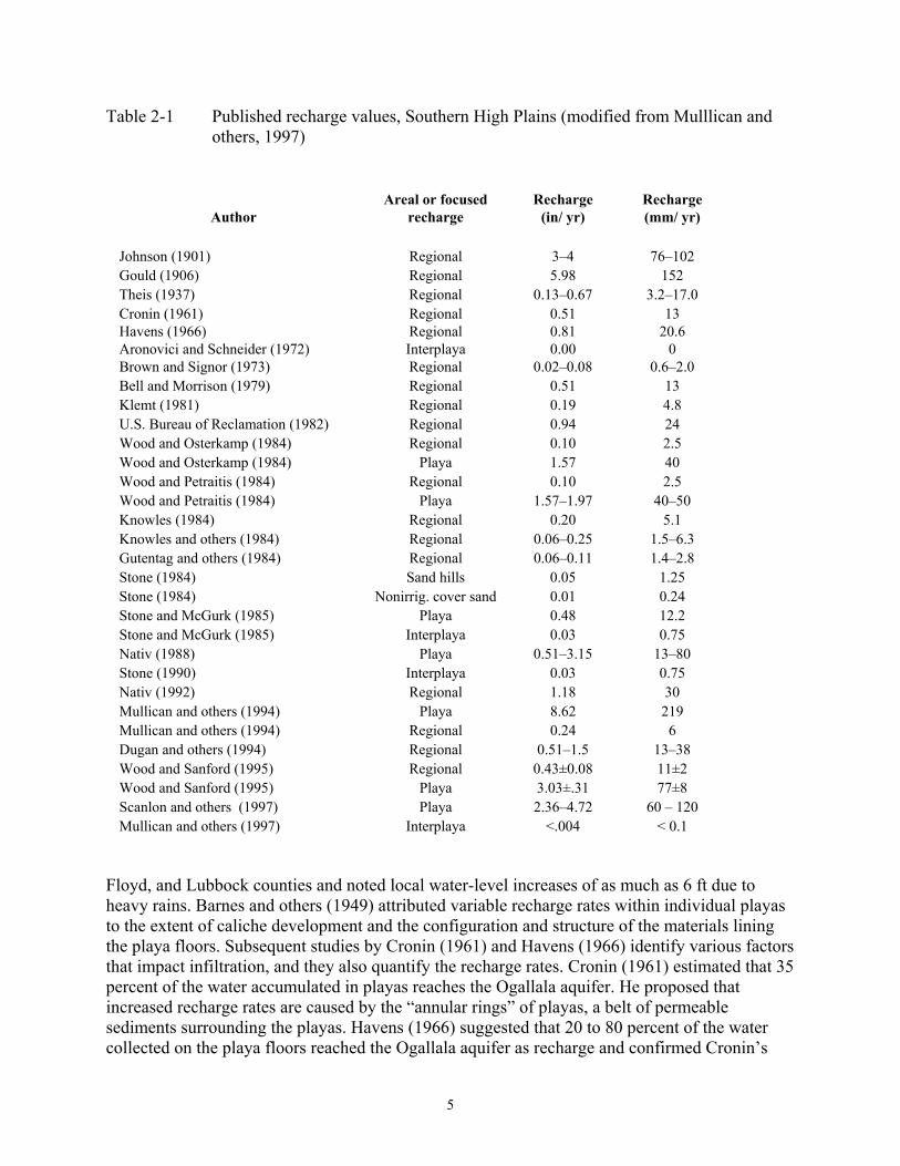
Table 2-1 Published recharge values, Southern High Plains (modified from Mulllican and others, 1997)

Author

Areal or focused recharge

Recharge (in/ yr)

Recharge (mm/ yr)

Johnson (1901) Regional 3–4 76–102 Gould (1906) Regional 5.98 152 Theis (1937) Regional 0.13–0.67 3.2–17.0 Cronin (1961) Regional 0.51 13 Havens (1966) Regional 0.81 20.6 Aronovici and Schneider (1972) Interplaya 0.00 0 Brown and Signor (1973) Regional 0.02–0.08 0.6–2.0 Bell and Morrison (1979) Regional 0.51 13 Klemt (1981) Regional 0.19 4.8 U.S. Bureau of Reclamation (1982) Regional 0.94 24 Wood and Osterkamp (1984) Regional 0.10 2.5 Wood and Osterkamp (1984) Playa 1.57 40 Wood and Petraitis (1984) Regional 0.10 2.5 Wood and Petraitis (1984) Playa 1.57–1.97 40–50 Knowles (1984) Regional 0.20 5.1 Knowles and others (1984) Regional 0.06–0.25 1.5–6.3 Gutentag and others (1984) Regional 0.06–0.11 1.4–2.8 Stone (1984) Sand hills 0.05 1.25 Stone (1984) Nonirrig. cover sand 0.01 0.24 Stone and McGurk (1985) Playa 0.48 12.2 Stone and McGurk (1985) Interplaya 0.03 0.75 Nativ (1988) Playa 0.51–3.15 13–80 Stone (1990) Interplaya 0.03 0.75 Nativ (1992) Regional 1.18 30 Mullican and others (1994) Playa 8.62 219 Mullican and others (1994) Regional 0.24 6 Dugan and others (1994) Regional 0.51–1.5 13–38 Wood and Sanford (1995) Regional 0.43±0.08 11±2 Wood and Sanford (1995) Playa 3.03±.31 77±8 Scanlon and others (1997) Playa 2.36–4.72 60 – 120 Mullican and others (1997) Interplaya <.004 < 0.1

Floyd, and Lubbock counties and noted local water-level increases of as much as 6 ft due to heavy rains. Barnes and others (1949) attributed variable recharge rates within individual playas to the extent of caliche development and the configuration and structure of the materials lining the playa floors. Subsequent studies by Cronin (1961) and Havens (1966) identify various factors that impact infiltration, and they also quantify the recharge rates. Cronin (1961) estimated that 35 percent of the water accumulated in playas reaches the Ogallala aquifer. He proposed that increased recharge rates are caused by the “annular rings” of playas, a belt of permeable sediments surrounding the playas. Havens (1966) suggested that 20 to 80 percent of the water collected on the playa floors reached the Ogallala aquifer as recharge and confirmed Cronin’s

5

(1961) theory of increased percolation rates through the permeable playa slopes. According to Havens (1966), seepage from irrigation also contributes to the overall recharge. Clyma and Lotspeich (1966) agreed that playa lakes were the principal source of aquifer recharge but thought that the infiltration amounts suggested by Havens (1966) and Cronin (1961) were too high. On the basis of a comparison of pan evaporation rates and volumetric changes measured in water ponding in a Bushland playa, Clyma and Lotspeich (1966) estimated that only 15 percent of the water in the lake reaches the aquifer. This estimate contrasted with an earlier estimate by Reddell and Rayner (1962), who reported that at five playa lakes around Lubbock, 54 to 84 percent of the surface water reached the Ogallala aquifer.

The conceptual model of recharge to the Ogallala aquifer changed markedly in the mid-1960s through about 1980. During this period, recharge through playas was thought to be negligible because of thick clay soils, and playas were considered evaporation pans. Ward and Huddleston (1972) looked at the impact of local playa geology on downward percolation of water and concluded that infiltration rates in 11 Lubbock County playa lakes were strongly dependent on the clay content in the top foot of soil. The authors estimated that about 90 percent of surface water evaporated, whereas the remainder percolated through the playa floor at a sharply declining rate before reaching a steady state. Bell and Sechrist (1972) also concluded that most of the playa water was being lost to evaporation so that “water in the shallow lakes could only be expected to remain for a few days.” However, in 1979, Bell and Morrison argued that changes in the topsoil structure caused by recent agricultural practices led to higher and faster aquifer recharge. A 1982 report by the U.S. Bureau of Reclamation concluded that although playa lakes are the largest contributors of recharge to the Ogallala aquifer, most of the water that accumulates in them is lost through evaporation. Field-monitoring techniques and satellite imagery were used to determine the percentage of High Plains playa lakes that held water in the wet and dry periods. The authors discovered that 15 percent of the playas held water during the wet period and 2 percent of the playas held water during the dry season.

Beginning in the early 1980s, the conceptual model of recharge to the Ogallala aquifer reverted to the original model of the system, which indicated that playas focus recharge. Wood and Osterkamp (1984, 1987) conducted detailed studies of recharge to the Ogallala aquifer. They used historical water-level records, tritium data, vadose-zone geochemistry under playa and interplaya settings, lake-water chemistry, vegetation data, chloride mass-balance profiles, and water-budget studies. Wood and Osterkamp (1987) proposed that most infiltration occurs through the annulus surrounding the playa. Wood and Petraitis (1984) monitored groundwater levels after rainfall events and investigated pore-water chemistry in the unsaturated zone. They concluded that Ogallala aquifer recharge occurs predominantly through playas. Stone (1984, 1990) and Stone and McGurk (1985) used the soil-water chloride mass-balance approach in playas and interplayas to estimate recharge rates. They concluded that playa lakes furnish most of the recharge and that nonirrigated interplaya areas had the lowest recharge rates. Nativ (1988) studied the isotopic composition of groundwater below playa lakes and concluded that the Ogallala aquifer is most likely recharged by focused percolation of partly evaporated playa-lake water rather than by slow, regional, diffusive percolation of precipitation. On the basis of chemical and isotopic data in the Southern High Plains, Nativ (1992) suggested recharge rates of 1.2 inches/year to the Ogallala aquifer. Mollhagen and others (1993) evaluated the potential for nonpoint source pollution at 99 playa lakes in the Brazos River Basin by comparing the levels of chloride in local precipitation with chloride concentrations in soil water. Their results suggest

6

that playa lakes are flushing chloride through the vadose zone, thus recharging the aquifer. Scanlon and Goldsmith (1997) and Scanlon and others (1997) conducted a detailed study to quantify spatial variability in recharge beneath playa and interplaya settings. Water contents, water potentials, and tritium concentrations were much higher and chloride concentrations were much lower beneath playas than in interplaya settings, which indicated that playas focus recharge. The results refute previous hypotheses that playas act as evaporation pans or that recharge is restricted to the annular region around playas. Water fluxes estimated from environmental tracers ranged from 2.4 to 4.7 inches/year beneath playas and <0.004 inches/year beneath natural interplaya settings not subjected to ponding or irrigation. To reconcile the apparent inconsistency between high recharge rates and thick clay layers beneath playas, ponding experiments were conducted, which showed preferential flow along roots and desiccation cracks through structured clays in the shallow subsurface in playas. Wood and others (1997) used a water-budget approach combined with chemical data to show that 60 to 80 percent of recharge to the Ogallala aquifer occurs through macropore flow. Mullican and others (1997) numerically simulated groundwater flow and showed that the playa-focused recharge theory is hydrologically plausible.

Other researchers (Knowles and others, 1984; Weeks and Gutentag, 1984) suggested that recharge to the Ogallala aquifer occurs chiefly by infiltration of precipitation on formation outcrops and streams’ seepage, thus discounting the playa theory. Knowles and others (1984) indicated that the caliche layers overlying the Ogallala aquifer may impede recharge and emphasized that the recharge rates are not uniform but vary as a function of local soil composition. Stone (1990) also concluded that water reaches the aquifer by infiltration through dry channels.

2.1.2 Enhanced Recharge

The possibility of using water ponding in playas to enhance recharge to the Ogallala aquifer has been considered since it became clear that more groundwater was being removed from the aquifer than was being returned through natural recharge. Numerous field experiments, dating back at least to 1955, have been undertaken to test the feasibility of enhancing recharge of groundwater. The most popular methods of enhanced recharge were (1) the use of water-spreading basins from which water infiltrates to the water table and (2) the use of injection wells to pump water into the aquifer. The most common problem encountered with the use of surface runoff water was clogging of the recharge basins by the sediments suspended in the water. Dvoracek and Peterson (1971) achieved recharge rates of as much as 1.5 ft per day from pits located on the outer perimeter of a playa near Lubbock. However, continued infiltration of high-sediment-content waters reduced rates to 0.1 ft per day. The authors concluded, “some clarification of water is required for economical and efficient artificial recharge.”

Aronovici and others (1972) conducted several tests on recharge basins excavated beneath Pullman clay soils (depth ~4 ft) adjacent to a playa near Amarillo, Texas. Two model basins (A and B) were excavated. Each basin was 66 ft2 in area. Basin A was filled with turbid water from the nearby playa and was flooded for 65 days, whereas Basin B was filled with clear water and was flooded for 46 days. The flooding depth ranged from 1 to 1.5 ft. Initial water contents in the sediments were 0.19 ft3/ft3, and final water contents were 0.37 ft3/ft3. The wetting front advanced at about 0.45 ft/day in both basins. The percolation rate changed from 1.5 ft/day to 2.0 ft/day and

7

gradually increased to 4 ft/day on the 26th day. Percolation rates in Basin A decreased after that to a minimum of 1 ft/day because of surface sealing, whereas rates in Basin B continued to increase to 7 ft/day. The total percolation for Basin A was 147 ft in 65 days, and for Basin B was 196 ft in 46 days. As a result of these studies a 1-acre prototype basin (C) was built (Schneider and Jones, 1988) that was 660 ft long by 66 ft wide. The total recharge in Basin C was ~230 ft over 187 days (1.23 ft/day) various tests conducted between 1971 and 1978. The average recharge rate over this period was 0.37 ft/day. In contrast, excavation of a basin in a playa (Signor and Hauser, 1968) resulted in recharge rates that decreased to 1.5 inches/day because of low-permeability sediments. Various basin management techniques were also investigated, including scraping the surface and using organic mats. Corrugations up and down the slopes combined with a drain allowed the basin to recharge over the 7-year period without any other type of invasive management.

Irrigation return flow may also provide a significant amount of recharge to the Ogallala aquifer; however, studies have not been conducted specifically to quantify the contribution of irrigation return flow to recharge. Recharge from irrigation water may greatly exceed natural recharge in interplaya settings.

The current conceptual model of groundwater recharge in the Southern High Plains is that most recharge is focused beneath playas with very little recharge beneath interplaya settings. This fact would suggest that recharge should also be focused beneath reservoir impoundments. Studies of enhanced recharge indicate that basin modification can significantly increase recharge rates in playas (Aronovici and others, 1972). Similar modifications in reservoirs may also increase recharge beneath these reservoirs.

2.2 Site Description

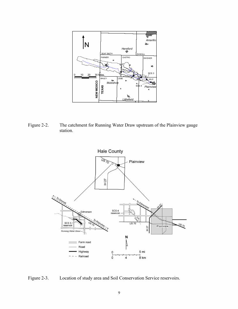
The study area is in the Running Water Draw catchment in the Southern High Plains region of Texas (Figures 2-2, 2-3). It is a subbasin of the Brazos River Basin and the uppermost headwater tributary of the Brazos River. Parts of Hale, Lamb, Swisher, Castro, and Parmer counties are within the basin. The basin land use and land cover are predominantly agricultural, and the upper part of the basin is in New Mexico. A USGS gauging station (08080700) is located in Plainview, Texas, which is the basin outlet. The drainage area upstream of the Plainview gauging station is 1,291 mi2. Daily flow records are available from 1939 through 1978. The average annual stream flow from 1939 to 1978 is 3.06 cfs, and maximum flow is 3,710 cfs. However, the records for 1954 and 195 are missing, and records for some years are incomplete.

Six SCS reservoirs were constructed along Running Water Draw for flood mitigation in Castro, Palmer, and Hale counties (Figure 2-2). Three of these reservoirs are located in northwestern Hale County. For this study, we focused on SCS 3 and SCS 4. The SCS 3 reservoir is located approximately 2.5 miles southeast of the city of Edmonson (Figure 2-3). It has a drainage area of about 28,000 acres. SCS 3 reservoir began operation on February 2, 1982. SCS 4 reservoir located approximately 3 miles west of Plainview and 1 mile north of State Highway 70 was placed on a tributary to Running Water Draw, which intercepts drainage from approximately 6,200 acres. SCS 4 reservoir began operation November 29, 1976. SCS 4 reservoir also receives irrigation return flow from nearby farm plots, and the floor of the reservoir is often muddy.

8

Plainview

Amarillo

Hereford

Littlefield

Muleshoe#

#

0 10 20 30 Miles $$

$$

$

$

LAMB HALE

DEAF SMITH

BAILEY

CASTROPARMER

RANDALL

SWISHER

NEW

MEX

ICO

TEXA

S

#

SCS 3

#

SCS 4

Figure 2-2. The catchment for Running Water Draw upstream of the Plainview gauge station.

Figure 2-3. Location of study area and Soil Conservation Service reservoirs.

9

Table 2-2. Areas, capacities, release rates, and conductivity data for SCS 3 and SCS 4 reservoirs. Average annual stream flow from 1939 to 1978 is 3.06 cfs, and maximum flow is 3,710 cfs. However, the records for 1954 and 1955 are missing, and records for some years are incomplete.

Emergency spillway Principal spillway (1) Principal spillway (2) Release rate (cfs)

Reservoir number Area

(acre) Capacity

(acre-feet) Area (acre)

Capacity (acre-feet)

Area (acre)

Capacity (acre-feet) (1) (2)

SCS 3 775 8,213 408 2,959 580 5,362 946 2,404 SCS 4 228 1,712 92 424 Only one spillway 95

0.0

5.0

10.0

15.0

20.0

25.0

1955 1960 1965 1970 1975 1979Year

(a)

QAc8106c

0.0

0.5

1.0

1.5

2.0

2.5

3.0

3.5

Jan Feb Mar Apr May Jun Jul Aug Sep Oct Nov DecMonth

(b)

Figure 2-4. Mean (a) annual and (b) monthly precipitation measured at the Hart weather station from 1955 through 1979.

Information on surface area, capacity, release rate, and estimated hydraulic conductivity of the reservoir floors is listed in Table 2-2. Local farmers report that historically more water was available from irrigation return flow in the 1970s and 1980s and SCS reservoirs were frequently filled during this time period. The drainage area upstream of the Plainview gauging station is 1,291 mi2. Daily flow records are available from 1939 through 1978. The average annual stream flow from 1939 through 1978 was 3.06 cfs, and maximum flow was 3,710 cfs. However, the records for 1954 and 1955 are missing, and records for some years are incomplete.

The climate is semiarid with long-term mean annual precipitation of 17.3 inches, according to precipitation records for Hart, Texas, collected from 1955 through 1979 (Figure 2-4). Rainfall is usually high during the summer months and peaks in June (Figure 2-4). A mapping study conducted by Texas Tech University indicates that the average playa surface area is about 19 acres (Fish and others, 1998). Playa lakes are concentrated in the study area (Figure 2-5). Table 2-3 lists the number and combined area of playa lakes in the counties in the Running Water Draw watershed. The depth to groundwater in the vicinity of the reservoirs ranges from 180 to 240 ft, according to a synoptic water-level survey conducted in January 2000.

10

Table 2-3. Playa statistics for the study area (from Fish and others, 1998).

County No. of playas Total playa floor area (acres)

Percent of county

Castro 610 19,100 3 Lamb 1,150 13,000 2 Hale 1,249 26,000 4

Parmer 433 9,800 1

Plainview

LAMB HALE

CASTRO SWISHER

0 5 10Mi

Figure 2-5. Location of playa lakes in the study area (from Fish and others, 1998).

11

3.0 Methods

A variety of different approaches were used to evaluate recharge beneath SCS reservoirs. Surface-water modeling was conducted by using the Soil and Water Assessment Tool (SWAT) (Arnold and others, 1994) to estimate surface-water inflow to the reservoirs. Field studies included electromagnetic induction to evaluate spatial variability in soil texture, salinity, or water content. Boreholes were drilled and soil samples analyzed for soil texture, water content, and chloride. Textural analyses were used to determine whether there is a surficial layer of fine- grained sediments that might greatly reduce infiltration beneath SCS reservoirs. Spatial variability in water content was used to estimate areas of low and high infiltration. Chloride concentrations in soil pore water were used to estimate infiltration rates. If chloride input to a system is uniform, then low chloride concentrations generally indicate high water fluxes as chloride is flushed out of the sediments, whereas high chloride concentrations indicate low water fluxes as chloride accumulates from evapotranspiration. Permeability tests were also conducted to determine whether permeability of the sediments increases with depth. Such analyses helped assess whether removal of surficial sediments would impact infiltration.

3.1 Surface-Water Modeling

Version 99.2 of SWAT (Neitsch and DiLuzio, 1999) that uses a Geographic Information System (GIS) interface (ArcView) was utilized in this study to evaluate surface runoff in the Running Water Draw catchment and to estimate the amount of water reaching the reservoirs. Surface-water simulations were conducted for 1950 through 1978 because of the availability of climatic data for that time period; the USGS surface-water gauge (8080700) was removed from Plainview in 1979. SWAT uses daily input data for the simulations. Stream flow was calibrated using gauge data from the USGS Plainview station.

The main features of SWAT are:

� Surface runoff from daily rainfall is predicted. Runoff volume is estimated with a modification of the SCS curve number method. The curve number varies nonlinearly from 1 (dry condition at wilting point) to 3 (wet condition at field capacity) and approaches 100 at saturation.

� Peak runoff rate predictions are based on a modification of the Rational Formula. The runoff coefficient is calculated as the ratio of runoff volume to rainfall. Rainfall intensity during the watershed time of concentration is estimated for each storm as a function of total rainfall by using a stochastic technique. The watershed time of concentration is estimated by using Manning’s Formula.

� The percolation component of SWAT uses a storage-routing technique to predict flow through each soil layer in the root zone.

� Lateral subsurface flow in the soil profile (0 to 6 ft) is calculated simultaneously with percolation. A kinematic storage model is used to predict lateral flow in each soil layer.

12

� The model offers three options for estimating potential evapotranspiration—Hargreaves, Priestley-Taylor, and Penman-Monteith. The temperature based Hargreaves equation was used for this study.

� Channel losses are a function of channel width and length and flow duration. Both runoff volume and peak rate are adjusted when transmission losses occur.

� The required inputs for ponds/reservoirs are capacity and surface area for emergency and principal spillways.

The weather inputs required by SWAT include daily precipitation and maximum/minimum air temperature. Daily solar radiation values were generated using monthly averages of the area. Daily wind speed and relative humidity were estimated in a similar manner.

To create a SWAT data set, the interface needs to access ArcView map themes and database files that provide certain types of information about the watershed. The Running Water Draw watershed delineation included a Digital Elevation Model (DEM) for the study area. The scale of the DEM was 1:250,000, where terrain elevations are recorded for ground positions on an evenly spaced grid at intervals of 328 ft. The SWAT ArcView interface delineates drainage basins on the basis of the principle that water always moves downhill. Streams are defined by specifying a minimum threshold drainage area that contributes flow to a particular channel. The accuracy of the watershed delineation was improved using a “burn-in” process. This process combines coverage of stream networks digitized from aerial photographs with the DEM to force the stream definition to agree more closely with reality. The DEM is shown in Figure 3-1. Digital maps of soils and land use are used to quantify a variety of watershed properties that control the relationship between rainfall and runoff. STATSGO soil coverages were obtained from the USDA NRCS (http://www.ftw.nrcs.usda.gov/stat_data.html). STATSGO map units are geographically referenced areas containing similar types of soils. On the basis of these map units, the SWAT ArcView interface derives important information, such as hydraulic conductivity and water-holding capacity for each subbasin.

There are two primary types of soils in the study area. Map unit TX055, which tends to follow the course of Running Water Draw, is characterized by a mixture of loam and clay-loam soils. These soils fall into hydrologic group B and have moderate infiltration rates. The other map units lying farther away from the stream have finer textures and lower infiltration rates. Map unit TX376, which comprises about 70 percent of the watershed, is categorized as hydrologic group C and has slow infiltration rates. The area just west of Plainview has claylike soils having very low infiltration rates (TX439). Figure 3-2 shows the STATSGO map units in the study area.

A grid of USGS land use and land cover classification codes was developed using land use/land cover maps downloaded from the Texas Natural Resources Information System. USGS classification codes are translated into SWAT land-cover types with defined hydrologic properties such as SCS curve numbers and leaf area indexes. More than 80 percent of the

study area is categorized as agricultural. Rangeland comprises another 15 percent. A map showing the location of different land cover types in the study area is provided in Figure 3-3.

13

LAMB HALE

DEAF SMITH

BAILEY

CASTROPARMER

RANDALL

SWISHERN

EW M

EXIC

O

TEXA

S

Elevation (feet)

3500 - 40004000 - 45004500 - 5000

3000 - 3500

Plainview

Figure 3-1. Topography of the catchment based on 1:250,000 DEM.

Historical precipitation and temperature data were input into the model. Observed daily data were obtained from the National Climatic Data Center (NCDC) weather database for seven stations in the vicinity of the study area (Figure 3-4). Precipitation data sets were compiled from observations at six stations, and temperature data sets were developed from measurements at two stations. Precipitation and temperature data for missing records were estimated statistically using monthly averages.

Surface-water simulations should generally be more accurate as the number of subwatersheds or hydrologic response units (HRUs) used increases. To examine the influence of different numbers of HRUs on the outflow hydrographs, the calculations were conducted using 9, 13, 17, 24, and 42 HRUs. The hydrographs simulated using different numbers of HRUs do not vary appreciably. Water-balance parameters, including average annual precipitation, water yield, recharge, evapotranspiration, and channel losses for each of the simulations, are listed in Table 3-1.

14

Figure 3-2. Soil cover data for the study area based on STATSGO.

Land Use CodeAGRLRNGE

Plainview

LAMB HALE

DEAF SMITH

BAILEY

CASTROPARMER

RANDALL

SWISHER

NEW

MEX

ICO

TEXA

S

STATSGO IDTX055TX376TX439TX440

LAMB HALE

DEAF SMITH

BAILEY

CASTROPARMER

RANDALL

SWISHER

NEW

MEX

ICO

TEXA

S

Figure 3-3. Spatial variability in land cover in the study area.

15

% Rainfall Data$ Temperature Dataÿ Statistical Data

%

%

%

%

%

%

$

$

$

ÿ

ÿ

LAMB HALE

DEAF SMITH

BAILEY

CASTROPARMERRANDALL

SWISHER

NEW

MEX

ICO

TEX

AS MULESHOE

HEREFORD

PLAINVIEW

DIMMITT

HART

FRIONA

MELROSE

Figure 3-4. Location of weather stations in the study area.

Table 3-1. Water balance results for the different densities of hydrologic response units (HRUs).

HRUs 9 13 17 24 42 Precipitation (inches) 1.63 1.64 1.642 1.639 1.641 Water yield (inches) 0.057 0.057 0.057 0.055 0.057 Recharge (inches) 0 0 0 0 0

ET (inches) 1.567 1.58 1.581 1.582 1.582 Channel losses (inches) 0.005 0.004 0.003 0.002 0.002

16

Because the simulations were not very sensitive to the number of HRUs, a total of 17 HRUs were used in the final simulations. The 15th HRU is the watershed outlet; the 16th and 17th HRUs were set at the SCS 3 and SCS 4 reservoirs. ArcView interface for SWAT 99.2 allows users to conduct reservoir routing by inserting a reservoir in a particular subbasin. Each subbasin can contain only a single reservoir. For reservoir inflow to be calculated, the reservoir location should be selected as the outlet of a subbasin. A reservoir subbasin cannot be delineated for an off-channel reservoir. The ArcView-SWAT interface allows only the outlet of a subbasin to be selected at river-channel locations that are delineated by the ArcView-SWAT interface. There is no stream delineated for the SCS 4 reservoir in this study; therefore, a subbasin for SCS 4 reservoir could not be delineated, and flow to this reservoir could not be calculated.

The model was calibrated by adjusting the SCS curve numbers until simulated and measured average annual stream flow was qualitatively modeled. The simulated flow was adjusted by modifying the SCS curve numbers for each of the HRUs. Initial estimates of SCS curve numbers were generated by SWAT.

3.2 EM Induction

Electromagnetic induction is a noninvasive technique that measures a depth-weighted average of the electrical conductivity called the apparent electrical conductivity (ECa) (McNeill, 1992). Because borehole data provide only point estimates of hydraulic and hydrochemical parameters, it is important to evaluate interborehole variability using noninvasive techniques such as electromagnetic induction. Apparent electrical conductivity measured by an electromagnetic meter varies with water content, salt content, sediment texture, structure, and mineralogy. A linear model can be used to describe variations in apparent conductivity (ECa) of the subsurface:

swa ECECEC += θτ (1)

where ECw is pore-water conductivity, θ is volumetric water content, τ is tortuosity, and ECs is surface conductance of the sediment (Rhoades and others, 1976). Variations in electrical conductivity may indicate spatial or temporal differences in infiltration. The various frequency- domain conductivity meters differ in the distances between the transmitter and receiver coils, the frequency at which they operate, and their effective exploration depths (Table 3-2). The instruments can be operated with transmitter and receiver coils horizontal (vertical dipole [VD] mode) or vertical (horizontal dipole [HD] mode). The EM31 and EM38 ground-conductivity meters (Geonics Ltd., Mississauga, Ontario) were used to measure ECa of the subsurface (McNeill, 1992). Apparent electrical conductivity was measured using surface EM meters along transects perpendicular to the margin of the reservoir (Figures 3-5, 3-6). Measurement locations were spaced 33 ft apart, and all measurements were taken at the ground surface in both the HD and VD orientations.

17

Table 3-2. Characteristics of electromagnetic induction conductivity meters including above ground EM38 and EM31 meters and the downhole EM39 meter used in this study (McNeill, 1992). Exploration depths for the different instruments correspond to approximately 70 percent of instrument response (McNeill, 1992).

Instrument Intercoil spacing (m)

Frequency (Hz)

Exploration depth (ft)

Horizontal dipole mode

Vertical dipole mode

Geonics EM38

1 14,600 2.46 4.92

Geonics EM31

3.7 9,800 9.84 19.68

Geonics EM39

0.5 39,200 Radial distance = 2.95 ft

QAc8109c

N

Dam centerline

GP3-1

GP3-2

GP3-3

GP3-4

GP3-5

GP3-9

GP3-8

GP3-7

Drain

M3-2

GP3-6GP3-10

M3-3

M3-1

A

B

A

A

A

A

BB

B

B

A

B

A

B

Mobile borehole (M)Ring infiltrometer testGuelph permeameter test (GP)EM transect

0 400 ft

Figure 3-5. Location of EM transects, boreholes (Giddings, Mobile), Guelph peremeameter tests, and ring infiltrometer tests in SCS 3 reservoir.

18

A QAc8110c

N

0 2

G4-1

G4-2

G4-6

G4-5

G4-3G 4-4

A

B

A

A

AA

A

A

A

B

B

B

B

B

B

B

B

M4-7

M4-8

M4-10

M4-9

Drain

Giddings probe boreholesMobile borehole (M)Water level transducerRing infiltrometer testEM transect

50 ft

Figure 3-6. Location of EM transects, boreholes, (Giddings, Mobile), and ring infiltrometer tests in SCS 4 reservoir.

19

3.3 Soil Texture, Water Content, and Chloride

A total of six boreholes were drilled at SCS 4 using a Giddings probe (Figure 3-6). The Giddings probe could not be used to drill boreholes beneath the SCS 3 reservoir because the soils were too dry. A Mobile rig was used to drill deeper boreholes in SCS 3 and SCS 4 reservoirs (Figures 3-5, 3-6). Because of ponding at the SCS 4 reservoir, these boreholes could not be drilled in the center of the reservoir. Cores were collected during drilling for analysis of soil texture, water content, and chloride concentration. Particle-size analyses were conducted on sediment samples from 13 boreholes (Table 3-3). Sediment samples from the initial shallow boreholes drilled by the Giddings probe in SCS 4 were not pretreated; however, all other samples were pretreated to remove carbonate. Percent sand, silt, and clay were determined by hydrometer analysis (Gee and Bauder, 1986), and sediment texture was classified according to the U.S. Department of Agriculture (1975) system. Gravimetric water content was measured on samples from 13 boreholes (Table 3-3), which were weighed the same day that they were collected as a precaution against sample drying before measurement.

Cores from 13 boreholes were sampled for chloride concentrations (Table 3-3). We extracted chloride from the pore water by adding double-deionized water to the dried sediment sample in a 3:1 ratio. Samples were agitated on a reciprocal shaker table for 4 hours. We then analyzed chloride in the supernatant by potentiometric titration using a 672 Titroprocessor and a 655 Dosimat (Metrohm, Inc., Switzerland) or by ion chromatography (Model 2010i chromatograph, Dionex Corp., Sunnyvale, California) on samples filtered through 0.45-µm filters.

3.4 Hydraulic Conductivity

Hydraulic conductivity is a critical parameter that controls infiltration of ponded water into the shallow subsurface and recharge to the underlying Ogallala aquifer. It is important to evaluate the spatial variability in hydraulic conductivity to determine future potential of SCS reservoirs to recharge the Ogallala aquifer. Depth variations in hydraulic conductivity provide valuable information on the feasibility of enhancing recharge by modifying surficial sediments in SCS reservoirs. Hydraulic conductivity was calculated from temporal variations in measured ponding depths in SCS 4, ring infiltrometer tests, and Guelph permeameter tests.

3.4.1 Reservoir Infiltration

Variations in water levels in SCS 4 reservoir may be considered a large infiltration test. The SCS 4 reservoir filled with water toward the end of March, and water levels declined until early June, when the reservoir refilled to a depth of about 8.6 ft. A pressure transducer was installed in early April toward the center of the reservoir to continuously monitor the stage at SCS 4 reservoir. The pressure transducer was attached to a data logger (Instrumentation Northwest), and water levels were monitored at 30-minute intervals. Pan-evaporation data were obtained from a meteorological station in Lubbock and were reduced by a factor of 0.7 to estimate lake evaporation. Water-level changes were corrected for evaporation to estimate net infiltration.

20

Table 3-3. Summary of boreholes drilled (G, Giddings drill rig; M, Mobil drill rig), date drilled, analyses conducted on soil samples, and tests conducted by Guelph permeameter tests.

SCS 3 reservoir Borehole number

Date drilled

Soil description Textural analysis

Water content

Chloride content

Guelph permeameter test

GP3-1 5/9/00 X X GP3-2 3/2/00 X X GP3-3 4/26/00 X X GP3-4 5/9/00 X X GP3-5 4/25/00 X GP3-6 4/26/00 X X GP3-7 5/10/00 X X GP3-8 4/25/00 X X GP3-9 5/10/00 X X

GP3-10 5/11/00 X X M3-1 7/11/00 X X X X M3-2 7/12/00 X X X X M3-3 7/13/00 X X X X

SCS 4 reservoir Borehole Soil description Textural

analysis Water content

Chloride Guelph permeameter test

GP4-1 2/29/00 X GP4-2 3/1/00 X GP4-3 2/21/00 X GP4-4 2/21/00 X G4-1 12/1/99 X X X G4-2 12/1/99 X X X G4-3 12/1/99 X X X G4-4 12/2/99 X X X G4-5 12/2/99 X X X G4-6 12/2/99 X X X M4-7 7/13/00 X X X X M4-8 7/13/00 X X X X M4-9 7/14/00 X X X X

M4-10 7/14/00 X X X X

21

3.4.2 Ring Infiltrometer Tests

The ring infiltrometer is a device used to calculate field-saturated hydraulic conductivity. A metal ring was driven into the ground and filled with water to a specified depth, which was maintained until infiltration reached steady state. Field-saturated hydraulic conductivity was calculated from the data. Data collected throughout the test included the volume of water released into the ring and the length of time required for the test. To visually inspect flow beneath the ponded area, a blue food coloring was added to the tanks containing the input water for the ring test. After each test, the ground under the test area was excavated using a backhoe, and the area of influence of the test was visually inspected and photographed. The ring used in the tests for this project was 3 ft in diameter by 2 ft in height. The ring was inserted into the ground to a depth of approximately 4 to 6 inches. During the test, the water input to the ring was monitored and controlled electronically. Two float switches were installed inside the ring to maintain a constant head of about 2 to 4 inches. Two test sites were selected in each reservoir, one at the surface and a second at depth (Figures 3-5, 3-6). At the SCS 3 reservoir the subsurface test was conducted at a depth of 2 ft, and at SCS 4 the test was conducted at a depth of 4 ft in the second site. The sites were selected to be representative of the reservoir as a whole. Each test was run for 24 hours or until infiltration stabilized. The field-saturated hydraulic conductivity was calculated using one-ponding-depth and two-ponding-depth approaches (Reynolds and Elrick, 1990).

3.4.3 Guelph Permeameter Tests

A Guelph permeameter Model 2800K1 was used to estimate the field-saturated conductivity of surficial sediments in the SCS 3 and SCS 4 reservoirs. The Guelph permeameter is an in-hole constant-head permeameter that is based on the Mariotte Principle. The method involves measuring the steady-state rate of water recharge into unsaturated soil from a cylindrical test hole in which a constant depth (head) of water is maintained. The tests were conducted by hand augering two, 4-inch-diameter boreholes to various depths. At approximately 1-ft intervals the borehole was cleaned using a sizing auger followed by a “well prep brush” to clean the borehole walls. The permeameter was inserted and centered in the boring, and the test was performed. After testing, the permeameter was removed, and the borehole was further advanced to repeat the procedure at various depths. Testing continued until a depth of 5 ft was reached or the borehole could no longer be advanced. Water heights of 2 and 4 inches were maintained during the tests. The flow rate from the permeameter was measured at timed intervals until a steady-state rate of fall was observed. The first test was conducted at 2 inches of water until a steady-state flow condition was observed, at which time the height of water was raised in the borehole to 4 inches. The test was completed when a steady-state flow rate was reached at 4 inches of water. Field-saturated hydraulic conductivity was determined on the basis of analysis of the data as described in Reynolds and Elrick (1985).

22

4.0 Results

Surface-water simulations demonstrate that the amount of water reaching the reservoirs exceeds the 200 acre-feet regulatory limit; therefore, increasing the storage capacity of the reservoirs should provide more water for recharge to the Ogallala aquifer. Water ponded in the SCS 4 reservoir during the study, whereas the SCS 3 reservoir remained dry. Ponding in the SCS 4 reservoir was attributed to irrigation return flow. Apparent electrical conductivity measured by the electromagnetic induction meters was higher beneath the SCS 4 reservoir than in the SCS 3 reservoir. Textural analysis of surficial sediments indicated that fine-grained sediments are found in the shallow subsurface of both SCS 3 and SCS 4 (~ upper 3 ft). Water contents in sediments were higher beneath the SCS 4 reservoir as a result of ponding. Chloride concentrations were low in both reservoirs, indicating that water percolates through the floors of the reservoirs. However, the rate could not be estimated using this method because of uncertainty in the chloride input to the system. Measurements of the stage in the SCS 4 reservoir during the study indicated that the average infiltration rate was 0.5 acre-foot/day. The average area that was ponded was 12.2 acres, which results in an average infiltration rate of 0.5 inch/day. Results of infiltration tests and hydraulic-conductivity tests indicated marked spatial variability in hydraulic conductivity and suggest that the best method of estimating the average infiltration rate is from monitoring water-level changes in the reservoir as a result of ponding.

4.1 Surface-Water Model Simulations

Observed stream flows are available from 1939 through 1978 for the USGS gauge (08080700) at Plainview, which excluded the missing years of 1954 and 1955. Observed precipitation is available from 1950 through 1979. Thus, the simulated period was selected from 1950 through 1978. The effect of playas on surface runoff was not simulated explicitly; however, the simulated runoff was reduced by the ratio of the catchment area of playas (382 mi2) to the catchment area of the entire basin (1,291 mi2). Precipitation and temperature data for individual weather stations were processed by the ArcView-SWAT interface to generate input files for the SWAT model. The SCS curve number was varied until good correspondence was found between measured and simulated flow in Plainview. Simulation generally reproduced the temporal variability in flow; however, the magnitude of the simulated flows differed from measured values. There is no obvious bias in the simulation results because peak flows are underestimated or overestimated at different times. Mean annual flow in 1960 in response to heavy precipitation was 13 cfs. The simulated mean annual stream flows at Plainview are shown in Figure 4-1.

Simulated flows at Plainview correspond fairly well with measured flows (root mean square error for annual flow from 1962 through 1978, 0.54 cfs). SWAT could not simulate flow to the SCS 4 reservoir because it is a tributary to Running Water Draw and not on the main channel. Simulated total annual inflow to the SCS 3 reservoir ranged from 1 acre-foot in 1976 to 9,380 acre-feet in 1951 (Table 4-1). The average total annual inflow from 1950 through 1978 was 2,180 acre-feet. These data indicate that the reservoirs can store much more water than the regulated 200 acre-feet. A subbasin for the SCS 3 reservoir was delineated, and the reservoir routing simulation was conducted. Comparison of simulated stream flows at SCS 3 with those at Plainview showed that the outflow hydrograph for the SCS 3 reservoir has exactly the same

23

QAc8105c

0

2

4

6

8

10

12

14

16

1945

Simulated Measured

1950 1955 1960 1965 1970 1975 1980Year

Figure 4-1. Simulated and measured mean annual stream flow for Running Water Draw in Plainveiw Texas.

Table 4-1. Simulated flows to SCS 3 reservoir.

SCS3

Year Annual Inflow rate (cfs)

Total annual Inflow

(acre-feet)

Year Annual Inflow rate (cfs)

Total annual Inflow

(acre-feet) 1950 3.67 2,658 1965 6.76 4,898 1951 12.96 9,380 1966 3.45 2,498 1952 1.02 737 1967 1.39 1,003 1953 2.37 1,715 1968 0.16 118 1954 2.99 2,164 1969 2.84 2,055 1955 1.56 1,128 1970 0.87 632 1956 0.32 230 1971 4.29 3,103 1957 1.28 925 1972 0.74 536 1958 0.71 513 1973 1.79 1,297 1959 5.06 3,667 1974 0.56 404 1960 11.33 8,223 1975 0.91 657 1961 10.41 7,539 1976 0.00 1 1962 2.05 1,487 1977 0.22 162 1963 5.68 4,115 1978 1.14 825 1964 0.75 545 Ave. 3.01 2,180

24

pattern as the hydrograph without reservoir routing. The timing and amplitude of peak flows in the hydrograph were only slightly modified when the reservoir was included. The simulation results did not demonstrate the regulating effect of the reservoir on stream flow. The amplitude of the peaks should be reduced, and the timing of the peaks should be lagged relative to simulated hydrographs without a reservoir.

4.2 EM Induction

Apparent electrical conductivities (ECa) measured by the Geonics EM31 meter in SCS 3 were lower than those in SCS 4 by a factor of about 1.5 (mean EM 31 V: SCS 3, 27 mS/m; SCS 4, 44 mS/m; Figures 4-2, 4-3). Values of ECa in SCS 3 were generally uniformly low (Figure 4-2). The transect conducted outside the reservoir (3-6) had values of ECa that were similar to those of transects conducted within the reservoir (Table 4-2). Vertical variability in ECa can be evaluated by comparing EM38 and EM31 transects and vertical and horizontal dipole-mode transects. Values of ECa were higher in EM31 transects than in EM38 transects, suggesting increasing conductivity with depth. In addition, vertical dipole readings were slightly higher in horizontal than in vertical dipole mode, which is consistent with increasing conductivity with depth. Temporal variability in ECa in SCS 3 was also negligible. Transects were conducted at fivedifferent times from November 1999 through May 2000, and ECa values did not vary significantly (Table 4-2).

In contrast, values of ECa in SCS 4 were spatially variable and were highest toward the center of the reservoir and lowest near the margins of the reservoir (Figure 4-3). The mean value of ECa in the transect outside the reservoir (EM4-1; EM3-1 VD; 27 – 29 mS/m) was much lower than the mean values of ECa for all other transects (EM3-1 VD; 47 – 63 mS/m) (Table 4-2). High values of ECa in EM4-9 occur because water flows into the reservoir along a drainage in the vicinity of this transect. Conductivity transects were measured for only 3 months in this reservoir (November 1999 through February 2000) because this reservoir ponded in February. Values of ECa were fairly uniform over time (Table 4-2).

Variations in ECa can be attributed to differences in clay content and water content. Lower ECa values in SCS 3 relative to SCS 4 result from lower clay contents and corresponding lower water contents in this reservoir. Higher ECa values toward the center of the SCS 4 reservoir correspond to higher clay and water contents.

4.3 Soil Texture and Water Content

Sediments in the SCS 3 reservoir generally ranged from sandy loam to loamy sand with higher clay content in the upper 1 to 2 ft (Figure 4-4). Surficial sediments toward the center of the SCS 4 reservoir are much more clay rich (Figure 4-4), with the amount of clay generally ranging from 40 to 90 percent. The thickness of the fine-grained zone generally ranges from 1 to 3 ft. The dominant texture below this surficial fine-grained zone is sandy clay loam. Sediments in these

25

QAc8107cDistance (ft)VD HD

EM 3-7

0 100 200 300 400 500 600 700

EM 3-6

0 200 400 600 800 1000 1200

EM 3-2

0 100 200 300 400 500 600 700 800 900

EM 3-1

0 200 400 600 800 1000 1200

(a)

(b)

(c)

(d)

A B

AB

A B

A B

1030507090

1030507090

1030507090

1030507090

Figure 4-2. Apparent electrical conductivity measured using the EM 31 meter in the vertical and horizontal dipole mode. These graphs are from representative transects in SCS 3. For locations of transects see Figure 3-5.

26

Table 4-2. Mean apparent electrical conductivity for EM transects in SCS 3 and SCS 4 reservoirs. For location of transects, see Figures 3-5 and 3-6.

SCS 3

Mean Apparent Electrical Conductivity (mS/m) Trans. EM3-1 EM3-2 EM3-3 EM3-4 EM3-5 EM3-6 EM3-7 Nov-99 EM31 HD 24.1 23.6 28.0 - - - -

VD 27.2 27.1 31.8 - - - -

Dec-99 EM31 HD 25.2 23.7 31.5 22.1 22.5 24.2 22.3 VD 28.7 27.9 36.0 24.8 25.9 29.5 25.8

Feb-00 EM38 HD 17.2 24.3 24.3 18.3 22.9 16.8 23.8 VD 18.6 25.4 26.5 20.0 24.7 19.5 25.5 EM31 HD 25.2 22.5 30.6 21.4 22.2 24.1 22.7 VD 26.6 24.6 33.1 22.6 23.9 27.7 24.4 Apr-00 EM38 HD 21.7 21.0 22.3 17.8 20.7 16.9 19.6

VD 19.5 19.1 20.7 15.0 18.7 13.0 17.6 EM31 HD 29.2 25.7 35.6 25.2 24.2 28.8 25.8 VD 27.4 25.8 35.4 24.3 24.8 29.5 24.5 May-00 EM31 HD 24.3 22.1 30.8 20.7 21.7 22.8 21.2 VD 26.6 25.0 33.5 22.5 24.3 27.0 24.0 SCS 4 Mean Apparent Electrical Conductivity (mS/m) Nov-99 Trans. EM4-1 EM4-2 EM4-3 EM4-4 EM4-5 EM4-6 EM4-7 EM4-8 EM4-9

EM31 HD 24.1 50.6 - 53.8 - - - - - VD 29.3 50.9 - 50.7 - - - - -

Dec-99 EM31 HD 23.8 49.5 71.8 60.8 52.3 72.8 70.3 65.5 63.6 VD 29.3 51.6 61.5 55.9 55.0 62.5 61.1 54.8 55.2

Feb-00 EM38 HD 13.4 39.1 55.5 46.6 43.0 51.8 47.0 48.0 47.8 VD 14.3 40.7 56.4 47.7 46.1 54.8 47.6 47.6 51.1 EM31 HD 22.3 49.7 62.8 55.7 54.3 62.9 59.0 54.7 57.1

27

QAc8108c

EM31 VDEM31 HDEM38 VDEM38 HD

EM4-1

0 120 240 360 480 600

Distance (ft)

10

20

30

40

50

60

70

80

90

10

20

30

40

50

60

70

80

90

0 60 120 180 240 3000 120 240 360 480 600 720 840

0 120 240 360 480 600Distance (ft)

10

20

30

40

50

60

70

80

90

10

20

30

40

50

60

70

80

90

EM4-2

EM4-3 EM4-6

EM4-9

0 60 120 180 240 300 360 42010

20

30

40

50

60

70

80

90

480

(a) (b)

(c) (d)

(e)

A B

A

B

AB

A

B

A

B

Figure 4-3. Apparent electrical conductivity measured by using the EM 31 meter in the vertical and horizontal dipole mode. These graphs are from representative transects in SCS 4. For locations of transects see Figure 3-6.

28

QAc8104cTexture (percent) Water Content (g/g) Chloride (mg/L)

Borehole M3-1

Borehole M3-2

Borehole M3-3

0

10

20

30

40

0

10

20

30

40

0

5

10

15

20

Sand

Silt Clay

Sand

SiltClay

SandSilt

(a) (b) (c)

(d) (e) (f)

(g) (h) (i)

0 20 40 60 80 100 0 0.2 0.4 0.6 0.8 1.0 0 20 40 60 80 100

Figure 4-4. Profiles of soil texture, gravimetric water content, and chloride for boreholes in the SCS 3 reservoir. For location of boreholes see Figure 3-5.

shallow boreholes drilled with the Giddings rig were not pretreated to dissolve carbonate; therefore, silt and clay content may be higher than that in all the other profiles that were pretreated. The profiles toward the margins of the SCS 4 reservoir were much sandier, and the dominant texture is sandy loam.

Water contents in SCS 3 (mean: 0.09 to 0.15 g/g) were generally lower than those measured in SCS 4 (mean 0.10 to 0.49 g/g) (Table 4-3). The low water contents in the SCS 3 reservoir are similar to those from the deep profiles adjacent to the SCS 4 reservoir (mean 0.10 to 0.17 g/g). Water contents were higher in the upper 1 to 4 ft near the center of the SCS 4 reservoir (0.42 to 0.66 g/g). High mean water contents in profiles G4-3 and G4-6 result because these boreholes are shallow and the mean values are strongly weighted toward high water contents near the surface. Mean water contents generally decrease away from the center of the reservoir, and the deep profiles toward the margin of the reservoir have mean water contents ranging from the reservoir are uniformly low. These differences in water content are attributed to higher rates of water movement in the center of the ponded area and do not simply reflect variations in water storage associated with textural variations. Clay contents in surficial sediments were similar in G4-1 and G4-2; however, water contents were much higher in G4-2 than in G4-1. Below the shallow subsurface, water contents were lower and generally ranged from 0.1 to 0.3 g/g.

29

4.4 Chloride Tracer

Chloride concentrations in pore water from SCS 3 were generally low (mean 12 to 34 mg/L) relative to those in SCS 4 (mean 21 to 250 mg/L) (Table 4-3). The high mean chloride concentrations near the center of the SCS 4 reservoir generally reflect very high concentrations in the upper meter of sediments (mean Cl concentration: 29 to 478 mg/L), whereas mean chloride concentrations below this zone were as much as 10 times lower (mean 21 to 30 mg/L) (Figure 4-5). Chloride concentrations were uniformly higher throughout the profiles adjacent to the reservoir (M4-7 to M-10; mean: 42 to 77 mg/L) relative to those toward the reservoir center.

It is difficult to estimate water fluxes from the chloride data because of uncertainties in the chloride input to the system. The chloride concentration in ponded water in the SCS 4 reservoir was 12 mg/L, which is about 10 times higher than chloride concentrations in precipitation. Calculating water fluxes from chloride input from precipitation would result in a lower bounding estimate for water flux. If the chloride input to the system were uniform for both reservoirs, then variations in chloride concentrations in subsurface pore water would be inversely related to water flux and would suggest that water fluxes are higher beneath the SCS 3 reservoir.

4.5 Reservoir Infiltration

Variations in water levels in the SCS 4 reservoir (Figure 4-6) were used to estimate net infiltration, which should ultimately result in recharge to the Ogallala aquifer. Water levels in the 0.10 to 0.17 g/g (M4-7 through M4-10). Water contents in the deep profiles along the margins of SCS 4 reservoir ranged from 5.5 ft toward the end of March 2000 and decreased to 1.3 ft toward the end of May. They increased to a maximum of 8.6 ft at the beginning of June and decreased to 0.8 ft at the end of September. The cumulative increase in water level was 12.5 ft. Water levels were converted to water volumes by using relations between stage, area, and capacity from engineering specifications for the dam. The average maximum depth of water was calculated to be 2 ft. A total of 155 acre-feet ponded in the reservoir over the 6-month period from March through September 2000. About 55 acre-feet evaporated from the reservoir, and 100 acre-feet infiltrated. An average volume of 0.5 acre-foot/day inflitrated. The average area of the basin was estimated to be 12.2 acres; therefore, the average infiltration rate was about 0.5 inch/day. This infiltration rate is much lower than infiltration rates (~1 to 1.3 ft/day) recorded in basins modified to enhance recharge adjacent to playas described by Schneider and Jones (1988).

4.6 Hydraulic Conductivity

Ring infiltration tests were conducted at the SCS 3 and SCS 4 reservoirs. After the tests were completed, the area under the ring was excavated using a truck-mounted backhoe. In the SCS 3 reservoir the soil profile consisted of 12 inches of clay loam that graded into carbonate-rich clay. The zone of influence of the pond was 42 inches wide and 10 to 15 inches deep. The upper 2 to 3 inches of sediment was uniformly dyed, whereas below this zone, the dyed area looked mottled.

30

Tabl

e 4-

3.B

oreh

ole

num

ber,

mea

n pe

rcen

tage

val

ues o

f san

d, si

lt, a

nd c

lay;

mea

n an

d ra

nge

wat

er c

onte

nt, c

hlor

ide

conc

entra

tion,

and

car

bona

te c

onte

nt fo

r SC

S3 a

nd S

CS

4 re

serv

oirs

.

Tex

ture

%W

ater

Con

tent

(g/g

)C

hlor

ide

Con

tent

(ppm

)soi

l wat

er

Car

bona

te C

onte

nt

(%)

Bor

eho l

eM

ean

Sand

Mea

nSi

ltM

ean

Cla

yM

ean

Max

imum

Min

umum

Mea

nM

axim

umM

inum

umM

ean

Max

imum

Min

umum

G4-

135

.63

23.1

341

.25

0.18

0.26

0.06

20.8

560

.32

8.20

No

Dat

aN

o D

ata

No

Dat

aG

4-2

41.1

720

.00

38.8

30.

180.

560.

0061

.89

295.

5026

.24

No

Dat

aN

o D

ata

No

Dat

aG

4-3

15.7

517

.00

67.2

50.

460.

710.

1724

9.64

895.

0620

.71

No

Dat

aN

o D

ata

No

Dat

aG

4-4

48.0

015

.00

48.0

00.

170.

350.

0014

3.00

698.

8513

.04

No

Dat

aN

o D

ata

No

Dat

aG

4-5

49.0

015

.00

36.0

00.

220.

550.

1250

.33

351.

1516

.96

No

Dat

aN

o D

ata

No

Dat

aG

4-6

17.0

020

.00

62.0

00.

490.

790.

1313

.40

20.3

03.

40N

o D

ata

No

Dat

aN

o D

ata

M4-

160

.91

23.4

515

.64

0.12

0.19

0.05

42.4

959

.50

2.71

32.6

385

.38

3.12

M4 -

268

.46

22.5

49.

000.

100.

160.

0441

.69

74.3

716

.86

30.0

272

.50

3.50

M4 -

360

.06

26.1

99.

000.

170.

250.

0866

.36

182.

5429

.66

23.4

479

.40

3.50

M4-

459

.00

21.9

219

.08

0.11

0.17

0.04

77.4

116

4.14

12.0

526

.72

53.0

09.

70

M3 -

161

.64

22.9

115

.45

0.09

0.19

0.04

12.1

337

.69

1.90

26.7

223

.06

0.16

M3 -

277

.75

12.9

59.

300.

150.

320.

0634

.47

41.3

625

.25

27.1

954

.01

10.1

0M

3 -3

79.0

510

.14

10.8

10.

120.

240.

0221

.65

100.

122.

7117

.89

46.7

11.

02

31

31

02468

10

Sand Silt Clay

02468

10

Sand Silt Clay

0

1

2

3

4

Sand

Silt Clay

02468

10

SandClaySilt

Texture (percent)

02468

10

Water content (g/g)

Borehole G4-5

Borehole G4-4

Borehole G4-3

Borehole G4-2

Borehole G4-1

Chloride (mg/L)QAc8102(a)c

Sand

Silt

Clay

0 20 40 60 80 100 0 0.2 0.4 0.6 0.8 1.0 0 100 200 300 400

0 200 400 600 800

0 200 400 600 800 1000

0 100 200 300 400

0 20 40 60 10080

(a) (b) (c)

(d) (e) (f)

(g) (h) (i)

(j) (k) (l)

(m) (n) (o)

0 20 40 60 80 100 0 0.2 0.4 0.6 0.8 1.0

0 20 40 60 80 100 0 0.2 0.4 0.6 0.8 1.0

0 20 40 60 80 100 0 0.2 0.4 0.6 0.8 1.0

0 20 40 60 80 100 0 0.2 0.4 0.6 0.8 1.0

Figure 4-5. Profiles of soil texture gravimetric water content, and chloride for boreholes in the SCS 4 reservoir. For location of boreholes see Figure 3-6.

32

QAc8103c

Borehole G4-6

Borehole M4-1

Borehole M4-2

Borehole M4-3

Borehole M4-4

Sand

Silt Clay02

46

8

10

05

1015202530

05

1015202530

05

1015202530

05

1015202530

0 20 40 60 80 100Texture (percent)

0 0.2 0.4 0.6 0.8 1.0Water content (g/g)

0 50 100 150 200Chloride (mg/L)

0 50 100 150 200

0 20 40 60 80 10

0 20 40 60 80 100

0 20 40 60 80 10

Sand SiltClay

Sand

SiltClay

SiltClay

(a) (b) (c)

(d) (e) (f)

(g) (h) (i)

(j) (k) (l)

(m) (n) (o)

Sand

SiltClay

Sand

0

0

Figure 4-5. Continued.

33

QAc8117c

0

2

4

6

8

10

3/28/00 4/25/00 5/23/00 6/20/00 7/18/00 8/15/00 9/12/00 9/26/00

Figure 4-6. Variations in water levels in the SCS 4 reservoir from March through September 2000 and corresponding precipitation. Dashed line was estimated by projecting trend backward to the beginning of ponding.

Dye traveled along preferential pathways where the soil texture was coarser and, to a lesser extent, along root paths. Some areas within 4 inches of the surface received no dye because the material was very dense and compacted.

The ring infiltration test conducted at 2-ft depth in the SCS 3 reservoir had a sphere of influence 42 inches wide and 8 to 14 inches deep. The soil was a carbonate-rich clay. The dye again had a mottled appearance, but the flow paths were predominantly along roots that penetrated the clay. As the dye traveled along the roots, it seeped into the clay.

The ring test conducted at the surface in the SCS 4 reservoir consisted of a loamy clay 4-ft thick with silty clay at the base. The zone of influence of the test extended out 15 ft from the sides of the ring and penetrated to a depth of 1.5 to 3 ft. The first 6 inches of soil was uniformly dyed, whereas below this zone the dye moved along fractures and some rootlets. At a depth of 16 inches a low-permeability bedding surface resulted in lateral movement of water to a distance of 15 ft from the ring. Along this surface, the dye traveled back up to the surface in some places. The second test conducted at 4-ft depth showed that penetration of dyed water was restricted to the upper 0.25 inch of the clay material.

The ponding tests conducted at the surface in both reservoirs could not be analyzed using the two ponding-depth approaches because of the very small differences in flow rates at the two

34

Table 4-4. Results of ring infiltrometer tests. Depth of borehole, duration of test, diameter of borehole, H1 and H2 are ponding depths, Q1 and Q2 are infiltration rates corresponding to H1 and H2, respectively, Kfs is the field saturated hydraulic conductivity based on two-ponded depth analysis, and Kfs1 and Kfs2 are field saturated hydraulic conductivities based on one ponded depth analysis correspond to heads H1 and H2, respectively.

Location Depth Duration Diam. H1 H2 Q1 Q2 Kfs Kfs1 Kfs2 ft hr ft in in gal/min gal/min in/day in/day in/day

SCS 3 0 41 3 2.25 4.25 0.019 0.019 - 0.10 0.10 SCS 3 2 22 2 2.5 4.5 0.004 0.008 0.14 0.04 0.07

SCS 4 0 6 3 3.0 6.0 1.12 1.11 - 5.9 5.9 SCS 4 4 24 3 3.0 - - - - - -

ponded depths and the small negative changes in flow rates as the ponded depths increased. These tests were then analyzed using the single-ponding-depth approach (Table 4-4). An alpha value of 0.1/inch was used in the single-depth analyses and is the value for clay soil (Reynolds and Elrick, 1990). The resultant Kfs ranged from 0.1 to 6 inches/day. The relatively large Kfs value for the SCS 4 surface test was attributed to preferential flow, as evidenced by the subsurface distribution of blue dye beneath the ponded surface. The Kfs value for the ring-infiltration test conducted at 2-ft depth in SCS 3 ranged from 0.04 to 0.1 inch/day. In contrast, the ring-infiltration test conducted at 4-ft depth in SCS 4 indicates low permeability because water penetrated only 0.25 inch in 24 hours.

The results of the Guelph permeameter field-testing are provided in Table 4-5. The rate of water outflow generally ranged from 0.0 to 12.6 inches/minute. Steady-state flow was generally attained within 60 minutes. Calculated hydraulic conductivities using the Richards analysis ranged from 0.3 to 463 inches/day. Some tests resulted in negative values of Kfs because the analysis is not well conditioned; that is, the Kfs solution is dependent on the ratio of Q2 to Q1. These tests were analyzed using data from each head separately with the LaPlace analysis. The Guelph permeameter data suggest that there is no systematic variation in Kfs spatially (either with horizontal or vertical location). The high conductivities may result from preferential flow caused by cracking of the surficial sediments.

35

Table 4-5. Field saturated hydraulic conductivity results based on the Guelph permeameter measurements. Q1 and Q2 correspond to fluxes calculated from head measurements of 2 and 4 inches, respectively.

Depth Steady-state outflow rate (inches/min)

Kfs Richards eq. (inches/day)

Kfs LaPlace eq.

(inches/day)

Kfs LaPlace eq.

(inches/day) Test ID ft Q1 Q2 Kfs (2 inches

head) (4 inches

head) GP4-1 1.0 0.12 0.20 0.51

1.5 0.00 0.04 0.43 2.5 0.51 NA NA 0.06 NA 2.6 0.04 0.59 111.81

GP4-2 1.0 0.01 0.04 0.31 2.0 0.01 0.01 0.06 0.02

GP4-3 1.0 0.04 0.06 1.50 2.0 0.06 0.16 16.57 2.8 0.06 0.12 8.39

GP4-4 1.0 0.08 0.14 0.43 2.0 0.10 0.10 0.51 0.02

GP3-1 1.0 0.04 0.06 1.50 2.2 0.06 0.12 8.39 3.2 0.04 0.06 1.50 4.3 0.02 0.24 2.65 5.4 0.20 0.30 7.48

GP3-2 1.0 0.20 0.43 36.14 2.0 0.10 0.24 22.17 2.6 0.08 0.12 2.99 3.9 No Flow No Flow 5.2 0.04 0.10 9.69

GP3-3 1.0 0.02 0.04 2.80 2.0 0.02 0.02 1.81 0.67 3.0 0.08 0.20 19.37 3.9 0.01 0.24 12.68 8.15 5.1 0.10 0.22 18.07

GP3-4 1.1 1.33 1.81e 20.79e 2.2 7.02 CNE 651.97 3.2 7.80 12.60e 463.39 724.41 435.83 4.3 CNE CNE 4.9 4.29e 5.51 398.43e 190.55

GP3-5 1.0 0.06 0.14 12.48 2.0 0.06 0.12 8.39

36

Table 4-5. Continued.

Depth Steady-state outflow rate (inches/min)

Kfs Richards eq. (inches/day)

Kfs LaPlace eq.

(inches/day)

Kfs LaPlace eq.

(inches/day) Test ID ft Q1 Q2 Kfs (2 inches

head) (4 inches

head) GP3-5 3.2 0.04 0.04 3.62 1.34

4.1 0.14 0.43 52.36 GP3-6 1.0 0.06 0.06 5.43 2.05

2.0 0.62 0.79 57.87 27.17 3.0 CNE CNE 3.9 CNE CNE 5.1 CNE CNE

GP3-7 1.1 0.14 0.30 23.66 2.2 0.39 0.55 6.81 3.2 1.40e 2.01e 29.37e 5.4 CNE CNE

GP3-8 1.0 0.16 0.24 5.98 2.0 0.16 0.30 18.27 3.0 0.08 0.12 2.99 4.3 3.32 CNE NA 307.87 4.6 0.39 0.98e 96.85e

GP3-9 1.0 0.08 0.10 7.24 3.39 2.0 0.10 0.14 1.69 3.2 0.12 0.20 8.58 4.3 0.16 0.30 29.06 5.4 0.55 0.79 12.80

GP4-10 1.1 0.86e 79.53e 2.2 1.95e CNE 181.10e 3.2 4.29e CNE 398.43e 4.3 1.56e CNE 144.88e

CNE = Could Not Establish a rate

e = estimate

37

5.0 Discussion

Results of this study suggest that current recharge is higher in the SCS 4 reservoir than in the SCS 3 reservoir. Analysis of water levels after ponding in the reservoir, high apparent electrical conductivities, and high water contents in subsurface sediments are evidence of recharge in the SCS 4 reservoir. Water-level fluctuations, indicating that 100 acre-feet of water infiltrated over a 6-month period, provide the most direct evidence of net infiltration and recharge. The average maximum depth of water was calculated to be 2 ft. The calculated average infiltration rate was about 0.5 inch/day. The volume of recharge in the SCS 4 reservoir is attributed to large amounts of irrigation return flow reaching this reservoir. In contrast, current recharge in the SCS 3 reservoir is low, as shown by low apparent electrical conductivities and low water contents in subsurface sediments. Low chloride concentrations in pore water suggest that recharge rates were higher in the past when more irrigation was conducted in the vicinity of this reservoir.

Textural analysis of the sediments indicated a fine-grained zone in the upper 1 to 3 ft of the reservoirs. Surface-water modeling using the SWAT code indicated that high flow rates reach the SCS 3 reservoir, much greater than the regulated amount of water that can be stored in this reservoir (200 acre-feet). These data suggest that installing the plugs in these reservoirs could enhance recharge by increasing the amount of water available for recharge. Another possible mechanism of enhancing recharge would be to remove surficial (1- to 3-ft depth) fine-grained sediments; however, a single infiltration test conducted at 4-ft depth suggest very low conductivities occur below 3 feet depth. The current infiltration rates based on water-level fluctuations in the SCS 4 reservoir (0.5 inch/day) are low compared with calculated recharge rates in basins excavated adjacent to playas (Aronovici and others, 1972; Schneider and Jones, 1988).

6.0 Recommendations

To fully evaluate the potential for enhancing recharge by increasing the regulated storage capacity of SCS reservoirs and/or by modifying the surface of these would require additional studies. There are 62 SCS reservoirs in the Southern High Plains. Information on flow into these reservoirs would be required to assess the availability of water for recharge. Data on soils would be required to evaluate the permeability of subsurface sediments and the feasibility of modifying surficial sediments to increase subsurface permeability. Testing could be conducted at selected reservoirs that would include removal of surficial fine-grained sediments. Water levels in these reservoirs could be monitored to estimate evaporation and infiltration. Such field-scale testing is much more appropriate than conducting point-scale permeability tests and ring-infiltrometer tests because the effects of preferential flow and of heterogeneity could be averaged at the scale of the reservoir. Finally, the effect of enhancing recharge by altering SCS reservoirs could be compared with that achieved by altering playas. Studies conducted in playas near Amarillo, Texas, indicated that recharge rates could be increased markedly by removing surficial fine-grained sediments.

We recommend selecting at least two reservoirs from the 62 existing reservoirs to conduct an engineering feasibility analysis. Surficial sediments could be modified from the floor of these reservoirs to increase the infiltration rate. Plugs on these reservoirs could be installed to increase

38

the capacity of the reservoirs. Detailed monitoring could be conducted on these reservoirs to evaluate whether recharge had significantly increased and to quantify such recharge. Detailed surface-water modeling could be conducted to predict input to the reservoir. Monitoring may be required over several years to capture high-runoff events. Regional modeling could be conducted to assess the potential of runoff from surface drainages off the Southern High Plains. Such studies will help determine potential impacts of the proposed modifications of SCS reservoirs on downstream water users and lakes.

The approximately 20,000 playas in the Southern High Plains represent a much greater source of water than the 62 SCS reservoirs. More thorough studies examining the potential of enhancing recharge in playas should be conducted. One component of such studies could include numerical simulation of the field experiments previously conducted near Amarillo and additional modeling studies to explain recharge processes in playas. Geomorphic studies could be conducted to evaluate the distribution of different soil types in and adjacent to playas and their associated hydraulic properties. Playas could be selected for engineering feasibility studies similar to those described for SCS reservoir alterations. Results of such studies would provide the required information to determine whether playa modifications would greatly enhance recharge to the Ogallala aquifer. Regulatory approval may be required prior to conducting enhanced recharge studies in or adjacent to playas.

Future studies of playas could include a classification of playas based on Landsat imagery, including color IR photography. Using these data, workers could group playas according to the length of time they remain ponded with water. Those playas that are ponded most of the time should probably be excluded from recharge enhancements because they may function as effective wetlands. Similarly, playas that are ponded the least amount of time may also be excluded from recharge enhancements because they are probably effectively recharging the aquifer naturally. Recharge enhancement should concentrate on playas that fall in the midrange that is based on the length of time the playas are ponded. About 30 to 50 playas could be identified for recharge enhancements, and this identification would result in about one to two playas per county. If possible, duplicate playas could be identified that have similar characteristics. Recharge enhancement could be conducted at one of the two playas, and the effectiveness of enhancing recharge can be quantified by comparing the results with the recharge evaluation from the control playa. Recharge may be enhanced by removal of surficial fine-grained sediments. If these sediments are thick, trenches could be dug to penetrate the fine-grained zone.

7.0 Conclusions

The primary purpose of this study was to assess the recharge potential of SCS reservoirs and determine whether recharge could be enhanced by increasing the regulated storage capacity or modifying the surface of these reservoirs. Detailed studies were conducted at two reservoirs in Hale County, Texas. Results of surface-water modeling using the SWAT code indicate that large amounts of water may flow into these reservoirs (mean 2,180 acre-feet/year; range 1 to 9,380 acre-feet/year in the SCS 3 reservoir). The SCS 3 reservoir on the main Running Water Draw channel did not pond during the study, whereas ponding occurred in the SCS 4 reservoir on a tributary to Running Water Draw. Ponding in the SCS 4 reservoir is attributed to irrigation return

39

flow and runoff related to precipitation. EM induction and water-content data from boreholes indicate that subsurface-water fluxes beneath the SCS 3 reservoir are currently low, which is consistent with the lack of ponding. In contrast, EM induction and water-content data from the SCS 4 reservoir indicate wetter conditions and higher fluxes as a result of ponding. Low chloride concentrations in pore water beneath the SCS 3 reservoir suggest higher water fluxes in the past when irrigation return flow was greater. Analysis of stage data from the SCS 4 reservoir during the study suggests an average infiltration rate of about 0.5 inch/day. Hydraulic-conductivity tests conducted with blue dye tracer indicate preferential flow in surficial sediments and much lower conductivity at depth.

The results of this study indicate that recharge could be enhanced by increasing the storage capacity of the reservoirs beyond the currently regulated value of 200 acre-feet, which is based on surface-water modeling. Textural analysis indicates that there is a fine-grained zone in the upper 1 to 3 ft. Removal of this fine-grained zone may further increase recharge; however, the limited infiltration tests suggest that permeabilities at depth are low.

8.0 Acknowledgments

This work was conducted in accordance with the directive contained in Rider 13 in House Bill of the Texas Water Development Board appropriations from the 1999 Legislature. We are very grateful to the landowners, Mr. Fred Keese and Mr. Kevin Igo, for allowing us complete access to their properties. We thankfully acknowledge the invaluable assistance, guidance, and local insight of soil scientists Mr. Jimmy Lewis, United States Department of Agriculture (USDA), Natural Resource Conservation Service (NRCS) in Plainview, and Wilfred (Willie) Crenwelge, USDA, NRCS, in Lubbock. Dr. Phil Bennett, The University of Texas at Austin, Department of Geological Sciences, generously provided analytical expertise. MaryJo Schabel, University of Wisconsin, Department of Geography, provided analytical expertise as well. We also thank William F. Mullican III, Texas Water Development Board, for his guidance in successfully completing this project. We thank Doug Coker for his dedication and support during the drilling and field-testing. In addition, John Derton, Steve Moore, Randy Williams, and Texas Water Development Board staff provided valuable field and technical assistance. Tommy R. Knowles, Robert E. Mace, and Betsy Croker reviewed the manuscript. Adam Haynes, Special Assistant for Natural Resources, Office of the Speaker of the House, Texas Legislature, also reviewed the report.

40

9.0 References

Arnold, J. G., Williams, J. R., Srinivasan, R., and King, K. W., 1994, SWAT—Soil and Water

Assessment Tool: Texas A&M University, Blackland Research Center, Texas Agricultural

Experiment Station.

Aronovici, V. S., Schneider, A. D., and Jones, O. R., 1972, Basin recharging the Ogallala aquifer

through Pleistocene sediments, in Proceedings, Ogallala Aquifer Symposium: Texas Tech

University, International Center for Arid and Semiarid Land Studies, Special Report No. 39,

p. 182–192.

Baker, C. L., 1915, Geology and underground waters of the northern Llano Estacado: University

of Texas, Austin, Bureau of Economic Geology, Bulletin No. 57, 225 p.

Barnes, J. R., Ellis, W. C., Leggat, E. R., Scalapino, R. A., George, W. O., and Irelan, B., 1949,

Geology and ground water in the irrigated region of the Southern High Plains in Texas:

Texas Board of Water Engineers, Progress Report No. 7, 51 p.

Bell, A. E., and Morrison, S., 1979, Analytical study of the Ogallala aquifer in Carson County,

Texas, projections of saturated thickness, volume of water in storage, pumpage rates,

pumping lifts, and well yields: Texas Department of Water Resources, Report 242, 64 p.

Bell, A. E., and Sechrist, A. W., 1972, Playas, Southern High Plains of Texas, in Reeves, C. C.,

Jr., ed., Playa Basin Symposium: International Center for Arid and Semi-Arid Land Studies

and Department of Geosciences, Texas Tech University Publication No. 4, p. 35–39.

Broadhurst, W. L., 1942, Recharge and discharge of the ground-water reservoirs on the High

Plains in Texas: American Geophysical Union Transactions, v. 1, p. 9–15.

41

Brown, R. F., and Signor, D. S., 1973, Artificial recharge experiments and operations on the

Southern High Plains of Texas and New Mexico: U.S. Geological Survey, Water-Resources

Investigations 10-73, 54 p.

Clyma, W., and Lotspeich, F. B., 1966, Water resources in the High Plains of Texas and New

Mexico: U.S. Department of Agriculture, Agricultural Research Service, ARS 41-114, 14 p.

Cronin, J. G., 1961, A summary of the occurrence and development of ground water in the

Southern High Plains of Texas: Texas Board of Water Engineers Bulletin 6107, 104 p.

Dugan, J. T., McGrath, T., and Zelt, R. B., 1994, Water level changes in the High Plains

aquifer—predevelopment to 1992: U.S. Geological Survey, Water-Resources Investigations

Report 94-4027, 56 p.

Dvoracek, M. J., and Peterson, H. S., 1971, Development of systems for ground water recharge

into the Ogallala formation: Texas Tech University, Water Resources Center, WRC 71-4.

Fish, E. B., Atkinson, E. L., Mollhagen, T. R., Shanks, C. H., and Brenton, C. M., 1998, Playa

lakes digital database for the Texas portion of the playa lakes joint venture region: CD-

ROM and http://www.gstlab.rw.ttu.edu/playa.htm.

Gee, G. W., and Bauder, J. W., 1986, Particle-size analysis, in Klute, A., ed., Methods of soil

analysis, part 1, physical and mineralogical methods: Madison, Wisconsin, American

Society of Agronomy, Monograph No. 9, p. 383–410.

Gould, C. N., 1906, The geology and water resources of the eastern portion of the Panhandle of

Texas: U.S. Geological Survey, Water-Supply and Irrigation Paper No. 154, 64 p.

42

Gutentag E. D., Heimes, F. J., Krothe, N. C., Luchkey, R. R., and Weeks, J. B., 1984,

Geohydrology of the High Plains aquifer in parts of Colorado, Kansas, Nebraska, New

Mexico, Oklahoma, South Dakota, Texas, and Wyoming: U.S. Geological Survey Professional Paper

1400-B, 63 p.

Havens, J. S., 1966, Recharge studies on the High Plains in northern Lea County, New Mexico:

U.S. Geological Survey, Water-Supply Paper No. 1819-F, 52 p.

Johnson, W. D., 1901, The High Plains and their utilization: U.S. Geological Survey, 21st

Annual Report 1890–1900, part 4, p. 601–741.

Klemt, W. B., 1981, Evaluating the ground-water resources of the High Plains of Texas, neutron-

probe measurements of deep soil moisture as an indicator of aquifer recharge rates: Texas

Department of Water Resources, LP-142, 31 p.

Knowles, T. R., Nordstrom, P., and Klemt, W. B., 1984, Evaluating the ground-water resources

of the High Plains of Texas; records of wells and maps showing locations, base of aquifer,

water levels, and saturated thickness: Texas Department of Water Resources, Report 288,

475 p.

McNeill, J. D., 1992, Rapid, accurate mapping of soil salinity by electromagnetic ground

conductivity meters, in Topp, G. C., and Reynolds, W. D., eds., Advances in measurement

of soil physical properties bringing theory into practice: Madison, Wisconsin, Soil Science

Society of America Special Publication 30, p. 209–229.

Mollhagen, T. R., Urban, L. V., Ramsey, R. H., Wyatt, A. W., McReynolds, C. D., and Ray,

J. T., 1993, Assessment of non-point source contamination of playa basins in the High

Plains of Texas (Brazos River Watershed, Phase IP): Texas Tech University, Water

Resources Center, variously paginated.

43

Mullican, W. F., III, Fryar, A. E. and Johns, N. D., 1994a, Vertical transport of contaminants

through perched aquifers to the Ogallala aquifer, Pantex Plant area, Southern High Plains,

Texas, in Dutton, A. R., ed., Toxic substances and the hydrologic sciences: American

Institute of Hydrology, p. 547–562.

Mullican, W. F., III, Johns, N.D., and Fryar, A. E., 1994b, Calibration and sensitivity analysis of

an Ogallala aquifer ground-water flow model: The University of Texas at Austin, Bureau of

Economic Geology, milestone report prepared for the U.S. Department of Energy through

the Office of the Governor, State of Texas, 82 p.

1994c, What a difference a playa can make: defining recharge scenarios, rates and contaminant

transport to the Ogallala (High Plains) aquifer, in Urban, L. V., and Wyatt, A. W., ed.,

Proceedings of the Playa Basin Symposium, Texas Tech University, Lubbock, Texas, p.

97–106.

Mullican, W. F., III, Johns, N. D., and Fryar, A. E., 1997, Playas and recharge of the Ogallala

aquifer on the Southern High Plains of Texas-an examination using numerical techniques:

The University of Texas at Austin, Bureau of Economic Geology Report of Investigations

No. 242, 72 p.

Nativ, Ronit, 1988, Hydrogeology and hydrochemistry of the Ogallala aquifer, Southern High

Plains, Texas Panhandle and eastern New Mexico: The University of Texas at Austin,

Bureau of Economic Geology Report of Investigations No. 177, 64 p.

____________1992, Recharge into Southern High Plains aquifer—possible mechanisms,

unresolved questions: Environmental Geology & Water Sciences, v. 19, no. 1, p. 21–32.

Neitsch, S. L., and DiLuzio, M., 1999, ArcView interface for SWAT 99.2, user’s guide:

Blackland Research Center, Texas Agricultural Experiment Station.

44

Reddell, D. L., and Rayner, F. A., 1962, Multipurpose modification of playa sinks, part III,

hydrology and engineering, in U.S. Public Health Service, Lubbock City-County Health

Unit, High Plains Underground Water District, Texas Water Commission and others, first

annual progress report, project 29, p. 54–55.

Reynolds, W. D., and Elrick, D. E., 1985, In situ measurement of field-saturated hydraulic

conductivity, sorptivity, and the alpha-parameter using the Guelph permeameter: Soil Sci.,

v. 140, no. 4, p. 292–302.

____________1990, Ponded infiltration from a single ring: 1. Analysis of steady flow: Soil

Science Society of America Journal, v. 54, p. 1233–1241.

Rhoades, J. D., Raats, P. A. C., and Prather, R. J., 1976, Effects of liquid-phase electrical

conductivity, water content, and surface conductivity on bulk soil electrical conductivity:

Soil Science Society of America Journal, v. 40, p. 651–655.

Scanlon, B. R., and Goldsmith, R. S., 1997, Field study of spatial variability in unsaturated flow

beneath and adjacent to playas: Water Resources Research, v. 33, p. 2239–2252.

Scanlon, B. R., Goldsmith, R. S., and Mullican, W. F., III, 1997, Spatial variability in

unsaturated flow beneath playa and adjacent interplaya settings and implications for

contaminant transport, Southern High Plains, Texas: The University of Texas at Austin,

Bureau of Economic Geology Report of Investigations No. 243, 68 p.

Schneider, A. D., and Jones, O. R., 1988, Ground water recharge through excavated basins, in

Artificial Recharge of Ground Water Symposium: Anaheim, California, Irrigation Division

of American. Society of Civil Engineers, p. 292–301.

45

Signor, D. C., and V. L. Hauser, 1968, Artificial ground water recharge through basins in the

Texas High Plains: Texas Agricultural Experiment Station Miscellaneous Publication 895,

8 p.

Stone, W. J., 1984, Preliminary estimates of Ogallala-aquifer recharge using chloride in the

unsaturated zone, Curry County, New Mexico, in Whetstone, G. A., ed., Proceedings,

Ogallala Aquifer Symposium II: Texas Tech University, Water Resources Center, p. 376–

391.

____________1990, Natural recharge of the Ogallala aquifer through playas and other non-

stream-channel settings, Eastern New Mexico, in Gustavson, T. C., ed., Geologic

framework and regional hydrology: upper Cenozoic Blackwater Draw and Ogallala

Formations, Great Plains: The University of Texas at Austin, Bureau of Economic Geology,

p. 180–192.

Stone, W. J., and McGurk, B. E., 1985, Ground-water recharge on the Southern High Plains, east

central New Mexico, in New Mexico Geological Society guidebook, 36th Field Conference,

p. 331–335.

Theis, C. V., 1937, Amount of ground-water recharge in the Southern High Plains: American

Geophysical Union Transactions, 18th Annual Meeting, p. 564–568.

U.S. Bureau of Reclamation, 1982, Llano Estacado playa lake water resources study: U.S.

Department of the Interior, Special Investigation, variously paginated.

U.S. Department of Agriculture, 1968, Work plan for watershed protection and flood prevention,

Lower Running Water Draw Watershed, Castro, Hale, Lamb, and Swisher Counties, Texas:

Fort Worth, Texas, U.S. Department of Agriculture-SCS, 54 p.

___________1975, Soil taxonomy: Washington, D.C., Soil Conservation Service, 754 p.

46

Ward, C. R., and Huddleston, E. W., 1972, in Reeves, C. C., Jr., ed., Playa Basin Symposium:

International Center for Arid and Semi-Arid Land Studies and Department of Geosciences,

Texas Tech University Publication No. 4, p. 203–286.

Weeks, J. B., and Gutentag, E. D., 1984, The High Plains regional aquifer-geohydrology, in

Whetstone, G. A., ed., Proceedings, Ogallala Aquifer Symposium II: Texas Tech University

Water Resources Center, p. 6–25.

White, W. N., Broadhurst, W. L., and Lang, J. W., 1946, Ground water in the High Plains of

Texas, in U.S. Geological Survey, Water-Supply Paper No. 889-F, p. 381–420.

Wood, W. W., and Osterkamp, W. R., 1984, Recharge to the Ogallala aquifer from playa lake

basins on the Llano Estacado (an outrageous proposal?), in Whetstone, G. A., ed.,

Proceedings, Ogallala Aquifer Symposium II: Texas Tech University, Water Resources

Center, p. 337–349.

____________1987, Playa-lake basins on the Southern High Plains of Texas and New Mexico:

part II, a hydrologic model and mass-balance arguments for their development: Geological

Society of America Bulletin, v. 99, p. 224–230.

Wood, W. W., and Petraitis, M. J., 1984, Origin and distribution of carbon dioxide in the

unsaturated zone of the Southern High Plains: Water Resources Research, v. 20, p. 1193–

1208.

Wood, W. W., Rainwater, K. A., and Thompson, D. B., 1997, Quantifying macropore recharge:

examples from a semi-arid area: Ground Water, v. 35, no. 6, p. 1097–1106.

Wood, W. W., and Sanford, W. E., 1995, Chemical and isotopic methods for quantifying

ground-water recharge in a regional, semiarid environment: Ground Water, v. 33, p. 458–

468.

47

49

App

endi

x I

Bor

ehol

e nu

mbe

r, sa

nd, s

ilt, c

lay

perc

enta

ges,

text

ural

cla

ssifi

catio

n, g

ravi

met

ric w

ater

con

tent

, chl

orid

e co

nten

t in

soil

sam

ples

, and

ch

lorid

e co

ncen

tratio

ns in

por

e w

ater

.

Bor

ehol

e D

epth

Sa

nd (%

) Si

lt (%

) C

lay

(%)

Soil

Tex

ture

W

ater

con

tent

(g/g

) PP

M C

L S

OIL

PP

M C

L H

20

G4-

1

0

1 17

82

cl

ay

0.21

12

.75

60.3

2 0.

5 18

17

65

cl

ay

0.26

6.

85

26.6

7 0.

7

0.

15

3.54

23

.21

0.9

0.16

2.

97

18.8

8 1.

1 30

28

42

cl

ay

0.23

4.

23

18.7

5 1.

4

0.

19

1.5

0.18

1.

8

0.

18

2

0.

18

3.63

20

.46

2.3

0.18

2.

5

0.

18

2.8

54

22

24

sand

y cl

ay lo

am

0.19

3.

96

21.3

1 3

0.19

3.

3

0.

18

3.5

0.17

3.

8 45

26

29

cl

ay lo

am

0.23

4.

68

20.4

3 4

0.22

4.

3

0.

21

4.5

0.21

2.

64

12.7

8 4.

8

0.

20

5 47

23

30

sa

ndy

clay

loam

0.

19

5.3

0.18

1.

62

9.06

5.

5

0.

18

5.8

0.17

6

0.16

6.

3

0.

16

6.5

0.17

6.

8

0.

16

50

Bor

ehol

e nu

mbe

r, sa

nd, s

ilt, c

lay

perc

enta

ges,

text

ural

cla

ssifi

catio

n, g

ravi

met

ric w

ater

con

tent

, chl

orid

e co

nten

t in

soil

sam

ples

, and

ch

lorid

e co

ncen

tratio

ns in

por

e w

ater

.

Bor

ehol

e D

epth

Sa

nd (%

) Si

lt (%

) C

lay

(%)

Soil

Tex

ture

W

ater

con

tent

(g/g

) PP

M C

L S

OIL

PP

M C

L H

20

G4-

1

7

49

24

27

sand

y cl

ay lo

am

0.16

1.

32

8.27

7.

2

0.

24

4.68

19

.24

7.4

0.21

7.

8

0.

15

1.74

11

.78

8 41

28

31

cl

ay lo

am

0.06

Mea

n 35

.625

23

.125

41

.25

0.

18

4.20

20

.86

M

in

0.06

1.

32

8.27

Max

0.

26

12.7

5 60

.32

G

4-2

0

2 9

89

clay

0.

19

55.0

1 29

5.50

0.

2

0.

52

34.8

8 67

.64

0.5

3 12

85

cl

ay

0.47

39

.54

83.7

4 0.

8 6

14

80

clay

0.

56

18.1

0 32

.59

1

0.

38

1.3

53

23

24

sand

y cl

ay lo

am

0.16

5.

77

36.4

6 1.

5

0.

17

1.8

53

22

25

sand

y cl

ay lo

am

0.19

2

0.18

2.

3

0.

17

2.5

57

18

25

sand

y cl

ay lo

am

0.14

4.

77

34.1

7 2.

8

0.

13

3

0.

13

3.5

0.15

3.

7

0.

15

3.95

59

17

24

sa

ndy

clay

loam

0.

15

5.01

32

.91

4.5

0.16

51

Bor

ehol

e nu

mbe

r, sa

nd, s

ilt c

lay

perc

enta

ges,

text

ural

cla

ssifi

catio

n, g

ravi

met

ric w

ater

con

tent

, chl

orid

e co

nten

t in

soil

sam

ples

, and

ch

lorid

e co

ncen

tratio

ns in

por

e w

ater

.

Bor

ehol

e D

epth

Sa

nd (%

) Si

lt (%

) C

lay

(%)

Soil

Tex

ture

W

ater

con

tent

(g/g

) PP

M C

L S

OIL

PP

M C

L H

20

G4-

2

5.

3

0.

17

5.5

0.16

5.

6 35

29

36

cl

ay lo

am

0.19

5.

64

29.4

0 5.

75

0.15

5.

95

0.13

6.

1

0.

16

6.3

49

26

25

sand

y cl

ay lo

am

0.14

4.

23

29.4

9 6.

6

0.

16

6.7

51

25

24

sand

y cl

ay lo

am

0.17

4.

53

26.2

4 6.

9

0.

16

7

0.

14

7.2

0.15

7.

3

0.

12

7.5

63

20

17

sand

y lo

am

0.10

4.

05

40.5

8 8

0.10

8.

2

0.

10

8.5

0.12

8.

7

0.

12

9.1

63

25

12

sand

y lo

am

0.12

4.

08

34.0

0 9.

2

0.

13

9.3

0.00

Mea

n 41

20

39

0.18

15

.47

61.8

9

Min

0.

00

4.05

26

.24

M

ax

0.56

55

.01

295.

50

G

4-3

0 4

11

85

clay

0.

17

155.

66

895.

06

52

Bor

ehol

e nu

mbe

r, sa

nd, s

ilt, c

lay

perc

enta

ges,

text

ural

cla

ssifi

catio

n, g

ravi

met

ric w

ater

con

tent

, chl

orid

e co

nten

t in

soil

sam

ples

, and

ch

lorid

e co

ncen

tratio

ns in

por

e w

ater

.

Bor

ehol

e D

epth

Sa

nd (%

) Si

lt (%

) C

lay

(%)

Soil

Tex

ture

W

ater

con

tent

(g/g

) PP

M C

L S

OIL

PP

M C

L H

20

G4-

3

0.

5 5

12

83

clay

0.

57

34.4

3 60

.86

1

0.

57

1.5

0.64

2

9 23

68

cl

ay

0.71

14

.71

20.7

1 2.

5

0.

32

3 45

22

33

cl

ay lo

am

0.23

5.

13

21.9

2

Mea

n 15

.75

17

67.2

5

0.46

52

.48

249.

64

M

in

0.17

5.

13

20.7

1

Max

0.

71

155.

66

895.

06

G

4-4

0

11

17

72

clay

loam

0.

28

42.3

9 15

2.51

0.

5

0.

35

22.6

9 65

.15

0.8

0.33

17

.07

50.9

9 1

14

20

66

clay

loam

0.

30

20.0

4 66

.27

1.2

0.35

1.

5

0.

33

1.7

0.34

2

13

23

64

loam

0.

32

5.25

16

.59

2.2

0.21

2.

5

0.

15

1.92

13

.04

2.7

43

20

32

clay

0.

19

3.13

16

.18

3

0.

17

3.2

0.15

3.

5

0.

13

3.7

62

16

22

clay

0.

12

3.51

28

.35

4 59

18

23

cl

ay

0.14

3.

72

25.7

3

53

Bor

ehol

e nu

mbe

r, sa

nd, s

ilt c

lay

perc

enta

ges,

text

ural

cla

ssifi

catio

n, g

ravi

met

ric w

ater

con

tent

, chl

orid

e co

nten

t in

soil

sam

ples

, and

ch

lorid

e co

ncen

tratio

ns in

por

e w

ater

.

Bor

ehol

e D

epth

Sa

nd (%

) Si

lt (%

) C

lay

(%)

Soil

Tex

ture

W

ater

con

tent

(g/g

) PP

M C

L S

OIL

PP

M C

L H

20

G4-

4

4.

2

0.

12

4.5

0.10

4.

7

0.

07

4.9

92

1 7

sand

y cl

ay

0.05

20

.94

434.

38

5

0.

06

5.2

0.08

5.

5

0.

08

5.7

0.07

6.

2

0.

11

6.4

89

3 8

sand

y cl

ay

0.11

6.

6

0.

00

2.96

69

8.85

M

ean

48

15

37

0.

17

13

143

M

in

0.00

1.

92

13.0

4

Max

0.

35

42.3

9 69

8.85

G4-

5

0

4 12

84

cl

ay

0.19

67

.57

351.

15

0.5

0.50

14

.40

28.7

6 0.

7 9

16

75

clay

0.

55

14.8

1 26

.95

1.2

33

14

53

clay

0.

42

7.92

18

.68

1.5

0.54

1.

7 9

24

67

clay

0.

55

9.37

17

.08

2

0.

33

2.2

0.19

2.

5 48

31

21

lo

am

0.18

3.

81

21.6

9 2.

7

0.

20

2.9

0.19

3.

2

0.

19

54

Bor

ehol

e nu

mbe

r, sa

nd, s

ilt, c

lay

perc

enta

ges,

text

ural

cla

ssifi

catio

n, g

ravi

met

ric w

ater

con

tent

, chl

orid

e co

nten

t in

soil

sam

ples

, and

ch

lorid

e co

ncen

tratio

ns in

por

e w

ater

.

Bor

ehol

e D

epth

Sa

nd (%

) Si

lt (%

) C

lay

(%)

Soil

Tex

ture

W

ater

con

tent

(g/g

) PP

M C

L S

OIL

PP

M C

L H

20

G4-

5

3.

5 70

5

25

sand

y cl

ay lo

am

0.19

3.

26

16.9

6 3.

7

0.

19

4

0.

16

4.2

0.16

4.

5

0.

15

4.7

0.16

5

70

8 22

sa

ndy

clay

loam

0.

17

3.33

19

.70

6

0.

16

6.2

0.18

6.

5 70

10

20

sa

ndy

clay

loam

0.

21

5.74

27

.58

6.7

0.19

6.

9

0.

17

7

0.

17

7.2

0.15

7.

5 78

7

15

sand

y lo

am

0.13

4.

08

31.2

1 7.

7

0.

16

7.9

0.17

5.

64

33.0

2 8

74

6 20

sa

ndy

clay

loam

0.

16

8.2

0.15

8.

5

0.

14

8.7

71

15

14

sand

y lo

am

0.14

4.

74

32.7

4 8.

9

0.

17

9.1

0.16

9.

4 57

27

16

sa

ndy

loam

0.

18

5.20

28

.76

9.6

0.12

55

Bor

ehol

e nu

mbe

r, sa

nd, s

ilt, c

lay

perc

enta

ges,

text

ural

cla

ssifi

catio

n, g

ravi

met

ric w

ater

con

tent

, chl

orid

e co

nten

t in

soil

sam

ples

, and

ch

lorid

e co

ncen

tratio

ns in

por

e w

ater

.

Bor

ehol

e D

epth

Sa

nd (%

) Si

lt (%

) C

lay

(%)

Soil

Tex

ture

W

ater

con

tent

(g/g

) PP

M C

L S

OIL

PP

M C

L H

20

G4-

5

Mea

n 49

15

36

0.22

11

.53

50.3

3

Min

0.

12

3.26

16

.96

M

ax

0.55

67

.57

351.

15

G

4-6

0 5

15

80

clay

0.

50

20.2

8 40

.36

0.5

2 11

87

cl

ay

0.68

12

.18

17.8

0 1

0.64

18

.56

28.9

7 1.

5

0.

63

2

0.

79

2.5

5 19

76

cl

ay

0.75

12

.90

17.2

8 3

3 20

77

cl

ay

0.66

13

.24

20.0

3 3.

5

0.

25

3.7

41

28

31

clay

loam

0.

13

3.43

27

.05

4.1

48

28

24

loam

0.

18

4.3

0.15

M

ean

17.3

3 20

.17

62.5

0.49

13

.43

25.2

5

Min

0.

13

3.43

17

.28

M

ax

0.79

20

.28

40.3

6

M3-

1

0.

00

42.0

0 26

.00

32.0

0 cl

ay lo

am

0.08

2.

97

37.6

9 1.

00

29.0

0 46

.00

25.0

0 lo

am

0.19

1.

07

5.71

2.

00

19.0

0 53

.00

28.0

0 si

lty c

lay

loam

0.

14

0.27

1.

90

3.00

23

.00

51.0

0 26

.00

silty

loam

0.

15

1.50

10

.19

4.00

41

.00

44.0

0 15

.00

loam

0.

11

1.19

10

.48

5.00

0.

06

56

Bor

ehol

e nu

mbe

r, sa

nd, s

ilt, c

lay

perc

enta

ges,

text

ural

cla

ssifi

catio

n, g

ravi

met

ric w

ater

con

tent

, chl

orid

e co

nten

t in

soil

sam

ples

, and

ch

lorid

e co

ncen

tratio

ns in

por

e w

ater

.

Bor

ehol

e D

epth

Sa

nd (%

) Si

lt (%

) C

lay

(%)

Soil

Tex

ture

W

ater

con

tent

(g/g

) PP

M C

L S

OIL

PP

M C

L H

20

M3-

1

5.

50

0.06

0.

31

5.07

6.

00

86.0

0 11

.00

3.00

lo

amy

sand

0.

05

0.72

14

.85

7.00

90

.00

5.00

5.

00

sand

0.

09

8.00

0.

10

1.24

12

.84

9.00

85

.00

2.00

13

.00

loam

y sa

nd

0.08

10

.00

0.06

0.

64

10.4

6 11

.00

86.0

0 6.

00

8.00

lo

amy

sand

0.

07

12.0

0

0.

07

13.0

0 88

.00

4.00

8.

00

loam

y sa

nd

0.07

14

.00

0.04

15

.00

89.0

0 4.

00

7.00

sa

nd

0.05

16

.00

0.06

M

ean

61.6

4 22

.91

15.4

5

0.09

1.

10

12.1

3

Min

0.

04

0.27

1.

90

M

ax

0.19

2.

97

37.6

9

M3-

2

0.00

4.

00

32.0

0 64

.00

clay

0.

32

7.47

23

.42

1.00

65

.00

25.0

0 10

.00

sand

y lo

am

0.17

5.

68

33.0

1 2.

00

61.0

0 30

.00

9.00

sa

ndy

loam

0.

17

9.87

58

.25

3.00

60

.00

32.0

0 8.

00

sand

0.

18

5.41

29

.64

4.00

91

.00

6.00

3.

00

sand

0.

08

4.72

59

.63

5.00

91

.00

3.00

6.

00

loam

y sa

nd

0.06

4.

77

83.9

1 5.

50

0.11

6.

50

87.0

0 5.

00

8.00

lo

amy

sand

0.

09

5.21

56

.37

8.00

0.

11

57

Bor

ehol

e nu

mbe

r, sa

nd, s

ilt c

lay

perc

enta

ges,

text

ural

cla

ssifi

catio

n, g

ravi

met

ric w

ater

con

tent

, chl

orid

e co

nten

t in

soil

sam

ples

, and

ch

lorid

e co

ncen

tratio

ns in

por

e w

ater

.

Bor

ehol

e D

epth

Sa

nd (%

) Si

lt (%

) C

lay

(%)

Soil

Tex

ture

W

ater

con

tent

(g/g

) PP

M C

L S

OIL

PP

M C

L H

20

M3-

2

9.

00

87.0

0 6.

00

7.00

sa

nd

0.11

10

.10

95.3

4 11

.00

90.0

0 7.

00

3.00

sa

nd

0.12

13

.00

0.12

5.

39

45.4

0 14

.00

91.0

0 4.

00

5.00

lo

amy

sand

0.

08

4.42

58

.91

16.0

0

0.

18

17.0

0 80

.00

15.0

0 5.

00

loam

y sa

nd

0.17

3.

93

23.6

7 18

.00

0.16

19

.00

79.0

0 16

.00

5.00

sa

ndy

loam

0.

19

4.91

26

.41

20.0

0

0.

18

21.0

0 74

.00

13.0

0 13

.00

sand

y lo

am

0.19

4.

98

26.5

1 22

.00

0.22

23

.00

81.0

0 14

.00

5.00

lo

amy

sand

0.

20

4.95

25

.25

24.0

0

0.

23

25.0

0

0.

16

26.0

0 84

.00

7.00

9.

00

loam

y sa

nd

0.11

4.

38

39.9

2 27

.00

0.12

28

.00

0.14

29

.00

89.0

0 8.

00

3.00

sa

nd

0.17

5.

33

30.4

8 30

.00

0.13

31

.00

0.13

32

.00

88.0

0 8.

00

4.00

sa

nd

0.13

4.

41

35.2

6 33

.00

0.13

34

.00

87.0

0 7.

00

6.00

lo

amy

sand

0.

13

5.28

41

.36

35.0

0

0.

14

36.0

0 85

.00

10.0

0 5.

00

loam

y sa

nd

0.13

37

.00

0.14

38

.00

81.0

0 11

.00

8.00

lo

amy

sand

0.

15

39.0

0

0.

09

2.98

34

.53

58

Bor

ehol

e nu

mbe

r, sa

nd, s

ilt c

lay

perc

enta

ges,

text

ural

cla

ssifi

catio

n, g

ravi

met

ric w

ater

con

tent

, chl

orid

e co

nten

t in

soil

sam

ples

, and

ch

lorid

e co

ncen

tratio

ns in

por

e w

ater

.

Bor

ehol

e D

epth

Sa

nd (%

) Si

lt (%

) C

lay

(%)

Soil

Tex

ture

W

ater

con

tent

(g/g

) PP

M C

L S

OIL

PP

M C

L H

20

M3-

2

M

ean

77.7

5 12

.95

9.30

0.15

4.

56

34.4

7

Min

0.

06

2.98

25

.25

M

ax

0.32

5.

33

41.3

6

M3-

3

1.00

9.

00

38.0

0 53

.00

clay

0.

24

2.01

8.

35

2.00

50

.00

36.0

0 14

.00

loam

0.

20

2.07

10

.19

3.00

70

.00

23.0

0 7.

00

sand

y lo

am

0.15

2.

01

13.3

6 3.

80

81.0

0 13

.00

6.00

lo

amy

sand

0.

13

4.00

97

.00

1.00

2.

00

sand

0.

06

5.00

82

.00

6.00

12

.00

sand

y lo

am

0.11

6.

00

0.12

7.

00

87.0

0 4.

00

9.00

lo

amy

sand

0.

10

8.00

0.

09

2.19

22

.05

9.00

88

.00

3.00

9.

00

loam

y sa

nd

0.12

10

.00

0.16

11

.00

82.0

0 6.

00

12.0

0 sa

ndy

loam

0.

14

12.0

0

0.

13

1.59

11

.62

13.0

0 85

.00

5.00

10

.00

loam

y sa

nd

0.13

14

.00

0.10

1.

86

13.9

8 15

.00

91.0

0 1.

00

8.00

sa

nd

0.10

16

.00

0.10

1.

17

11.9

3 17

.00

89.0

0 2.

00

9.00

lo

amy

sand

0.

14

18.0

0

0.

15

1.41

9.

97

19.0

0 78

.00

13.0

0 9.

00

sand

y lo

am

0.16

20

.00

0.12

2.

82

18.1

0 21

.00

78.0

0 12

.00

10.0

0 sa

ndy

loam

0.

13

22.0

0

0.

16

2.37

18

.39

59

Bor

ehol

e nu

mbe

r, sa

nd, s

ilt c

lay

perc

enta

ges,

text

ural

cla

ssifi

catio

n, g

ravi

met

ric w

ater

con

tent

, chl

orid

e co

nten

t in

soil

sam

ples

, and

ch

lorid

e co

ncen

tratio

ns in

por

e w

ater

.

Bor

ehol

e D

epth

Sa

nd (%

) Si

lt (%

) C

lay

(%)

Soil

Tex

ture

W

ater

con

tent

(g/g

) PP

M C

L S

OIL

PP

M C

L H

20

M3-

3

23

.00

81.0

0 14

.00

5.00

lo

amy

sand

0.

13

24.0

0

0.

20

2.34

17

.40

25.0

0 75

.00

10.0

0 15

.00

sand

y lo

am

0.18

26

.00

0.

48

2.71

27

.00

87.0

0 4.

00

9.00

lo

amy

sand

0.

12

28.0

0

0.

02

29.0

0

0.

07

2.13

10

0.12

30

.00

31

.00

86.0

0 4.

00

10.0

0 lo

amy

sand

0.

09

32.0

0

0.

07

33.0

0 91

.00

5.00

4.

00

sand

0.

08

2.67

37

.62

34.0

0

0.

08

35.0

0 87

.00

6.00

7.

00

loam

y sa

nd

0.15

0.

58

7.53

36

.00

0.11

37

.00

0.08

38

.00

0.08

39

.00

86.0

0 7.

00

7.00

lo

amy

sand

0.

08

40.0

0

0.

05

2.34

29

.75

Mea

n 79

.05

10.1

4 10

.81

0.

12

1.87

21

.65

M

in

0.02

0.

48

2.71

Max

0.

20

2.82

10

0.12

M

4-1

0.00

49

.00

33.0

0 18

.00

loam

sa

mpl

e co

mpr

omis

ed

8.34

1.00

57

.00

26.0

0 17

.00

sand

y lo

am

sam

ple

com

prom

ised

2.

76

2.

00

47.0

0 25

.00

28.0

0 sa

ndy

clay

loam

sa

mpl

e co

mpr

omis

ed

1.53

60

Bor

ehol

e nu

mbe

r, sa

nd, s

ilt c

lay

perc

enta

ges,

text

ural

cla

ssifi

catio

n, g

ravi

met

ric w

ater

con

tent

, chl

orid

e co

nten

t in

soil

sam

ples

, and

ch

lorid

e co

ncen

tratio

ns in

por

e w

ater

.

Bor

ehol

e D

epth

Sa

nd (%

) Si

lt (%

) C

lay

(%)

Soil

Tex

ture

W

ater

con

tent

(g/g

) PP

M C

L S

OIL

PP

M C

L H

20

M4-

1

3.

00

51.0

0 24

.00

25.0

0 sa

ndy

clay

loam

4.00

52

.00

27.0

0 21

.00

sand

y cl

ay lo

am

sam

ple

com

prom

ised

2.

01

5.

00

64.0

0 15

.00

21.0

0 sa

ndy

clay

loam

6.00

7.00

0.

11

8.00

51

.00

34.0

0 15

.00

loam

0.

05

9.00

0.

12

10.0

0

0.

09

11.0

0 69

.00

20.0

0 11

.00

sand

y lo

am

0.10

6.

04

59.5

0 12

.00

0.15

13

.00

0.10

14

.00

66.0

0 24

.00

10.0

0 sa

ndy

loam

0.

14

15.0

0

0.

10

16.0

0

17.0

0 92

.00

6.00

2.

00

sand

0.

16

7.77

50

.03

18.0

0

0.

12

19.0

0

0.

19

20.0

0 72

.00

24.0

0 4.

00

sand

y lo

am

0.12

2.

20

17.9

3

M

ean

60.9

1 23

.45

15.6

4

0.12

4.

38

42.4

9

Min

0.

05

1.53

2.

71

M

ax

0.19

8.

34

59.5

0

M

4-2

0.00

61

.00

30.0

0 9.

00

sand

y lo

am

0.04

3.

18

72.0

7 1.

00

58.0

0 23

.00

19.0

0 sa

ndy

loam

0.

06

3.86

67

.84

2.00

47

.00

35.0

0 18

.00

loam

0.

08

2.64

33

.82

61

Bor

ehol

e nu

mbe

r, sa

nd, s

ilt, c

lay

perc

enta

ges,

text

ural

cla

ssifi

catio

n, g

ravi

met

ric w

ater

con

tent

, chl

orid

e co

nten

t in

soil

sam

ples

, and

ch

lorid

e co

ncen

tratio

ns in

por

e w

ater

.

Bor

ehol

e D

epth

Sa

nd (%

) Si

lt (%

) C

lay

(%)

Soil

Tex

ture

W

ater

con

tent

(g/g

) PP

M C

L S

OIL

PP

M C

L H

20

M4-

2

3.

00

45.0

0 31

.00

24.0

0 lo

am

0.09

1.

77

19.7

6 4.

00

52.0

0 35

.00

13.0

0 lo

am

0.13

5.

00

61.0

0 34

.00

5.00

sa

ndy

loam

0.

12

3.39

28

.16

6.00

0.

11

7.00

0.

11

8.00

79

.00

19.0

0 2.

00

loam

y sa

nd

0.11

1.

83

16.8

6 9.

00

0.09

10

.00

0.09

11

.00

74.0

0 19

.00

7.00

sa

ndy

loam

0.

10

2.93

28

.78

12.0

0

0.

11

13.0

0

0.

08

14.0

0 83

.00

15.0

0 2.

00

loam

y sa

nd

0.10

5.

06

48.2

8 15

.00

0.12

16

.00

0.11

17

.00

88.0

0 10

.00

2.00

sa

nd

0.11

3.

48

31.1

8 18

.00

0.10

19

.00

0.10

20

.00

69.0

0 20

.00

11.0

0 sa

ndy

loam

0.

05

3.78

74

.37

21.0

0

0.

09

22.0

0

0.

10

23.0

0 81

.00

16.0

0 3.

00

loam

y sa

nd

0.08

4.

05

50.5

2 24

.00

0.11

25

.00

0.10

26

.00

0.14

27

.00

92.0

0 6.

00

2.00

sa

nd

0.16

4.

63

28.5

9 28

.00

0.05

29

.00

0.14

62

Bor

ehol

e nu

mbe

r, sa

nd, s

ilt c

lay

perc

enta

ges,

text

ural

cla

ssifi

catio

n, g

ravi

met

ric w

ater

con

tent

, chl

orid

e co

nten

t in

soil

sam

ples

, and

ch

lorid

e co

ncen

tratio

ns in

por

e w

ater

.

Bor

ehol

e D

epth

Sa

nd (%

) Si

lt (%

) C

lay

(%)

Soil

Tex

ture

W

ater

con

tent

(g/g

) PP

M C

L S

OIL

PP

M C

L H

20

M4-

2

M

ean

68.4

6 22

.54

9.00

0.10

3.

38

41.6

9

Min

0.

04

1.77

16

.86

M

ax

0.16

8.

34

74.3

7

M

4-3

0.00

34

.00

33.0

0 33

.00

clay

loam

0.

18

9.86

53

.57

1.00

38

.00

35.0

0 27

.00

clay

loam

0.

21

37.5

7 18

2.54

2.

00

57.0

0 22

.00

21.0

0 sa

ndy

clay

loam

0.

12

8.63

72

.42

3.00

58

.00

25.0

0 17

.00

sand

y lo

am

0.13

10

.20

78.4

6 4.

00

53.0

0 33

.00

14.0

0 sa

ndy

loam

0.

15

9.22

62

.96

5.00

52

.00

38.0

0 10

.00

loam

0.

18

6.00

0.

21

7.00

57

.00

37.0

0 6.

00

sand

y lo

am

0.20

8.

90

44.9

0 8.

00

0.21

9.

00

47.0

0 46

.00

7.00

lo

am

0.25

7.

42

29.6

6 10

.00

0.17

11

.00

51.0

0 38

.00

11.0

0 lo

am

0.18

7.

53

41.5

7 12

.00

0.19

13

.00

62.0

0 29

.00

9.00

sa

ndy

loam

0.

17

8.10

48

.54

14.0

0

0.

13

15.0

0 74

.00

9.00

17

.00

sand

y lo

am

0.11

7.

22

63.9

5 16

.00

0.16

17

.00

77.0

0 9.

00

14.0

0 sa

ndy

loam

0.

17

7.92

47

.07

18.0

0

0.

13

19.0

0 74

.00

19.0

0 7.

00

sand

y lo

am

0.22

20

.00

0.21

21

.00

64.0

0 20

.00

16.0

0 sa

ndy

loam

0.

08

7.82

94

.41

22.0

0

0.

18

63

Bor

ehol

e nu

mbe

r, sa

nd, s

ilt, c

lay

perc

enta

ges,

text

ural

cla

ssifi

catio

n, g

ravi

met

ric w

ater

con

tent

, chl

orid

e co

nten

t in

soil

sam

ples

, and

ch

lorid

e co

ncen

tratio

ns in

por

e w

ater

.

Bor

ehol

e D

epth

Sa

nd (%

) Si

lt (%

) C

lay

(%)

Soil

Tex

ture

W

ater

con

tent

(g/g

) PP

M C

L S

OIL

PP

M C

L H

20

M4-

3

23

.00

0.24

24

.00

0.16

25

.00

73.0

0 18

.00

9.00

sa

ndy

loam

0.

14

7.73

54

.22

26.0

0

0.

16

27.0

0 90

.00

8.00

2.

00

sand

0.

14

7.65

54

.80

28.0

0

0.

12

Mea

n 60

.06

26.1

9 13

.75

0.

17

10.4

1 66

.36

M

in

0.08

7.

22

29.6

6

Max

0.

25

37.5

7 18

2.54

M

4-4

0.00

40

.00

33.0

0 27

.00

clay

loam

0.

08

12.7

8 16

4.14

1.

00

52.0

0 23

.00

25.0

0 cl

ay lo

am

0.08

8.

03

103.

52

2.00

44

.00

25.0

0 31

.00

sand

y lo

am

0.08

8.

62

103.

77

3.00

45

.00

21.0

0 34

.00

sand

y lo

am

0.09

7.

01

75.4

6 4.

00

48.0

0 27

.00

25.0

0 sa

ndy

loam

0.

10

7.49

75

.19

5.00

56

.00

22.0

0 22

.00

loam

0.

09

8.44

90

.73

6.00

0.

13

7.00

64

.00

22.0

0 14

.00

sand

y lo

am

0.12

7.

71

64.6

8 8.

00

0.09

9.

00

0.11

4.

15

39.4

5 10

.00

0.11

11

.00

61.0

0 23

.00

16.0

0 lo

am

0.13

1.

61

12.0

5 12

.00

0.13

13

.00

60.0

0 24

.00

16.0

0 lo

am

0.13

8.

54

64.8

6 14

.00

0.10

15

.00

64.0

0 19

.00

17.0

0 sa

ndy

loam

0.

05

64

Bor

ehol

e nu

mbe

r, sa

nd, s

ilt, c

lay

perc

enta

ges,

text

ural

cla

ssifi

catio

n, g

ravi

met

ric w

ater

con

tent

, chl

orid

e co

nten

t in

soil

sam

ples

, and

ch

lorid

e co

ncen

tratio

ns in

por

e w

ater

.

Bor

ehol

e D

epth

Sa

nd (%

) Si

lt (%

) C

lay

(%)

Soil

Tex

ture

W

ater

con

tent

(g/g

) PP

M C

L S

OIL

PP

M C

L H

20

M4-

4

16

.00

0.12

3.

86

31.3

1 17

.00

75.0

0 12

.00

13.0

0 sa

ndy

loam

0.

05

18.0

0

0.

11

16.8

2 15

1.95

19

.00

81.0

0 15

.00

4.00

sa

ndy

loam

0.

11

20.0

0

0.

13

6.98

53

.75

21.0

0 77

.00

19.0

0 4.

00

sand

y lo

am

0.11

22

.00

0.15

8.

11

52.8

7 23

.00

0.17

24

.00

0.04

Mea

n 59

.00

21.9

2 19

.08

0.

11

7.87

77

.41

M

in

0.04

1.

61

12.0

5

Max

0.

17

16.8

2 16

4.14

65

App

endi

x II

.

Sum

mar

y of

Run

ning

Wat

er D

raw

rese

rvoi

rs.

Pe

rmitt

ed

Low

Sta

ge

Cou

nty

Dam

Nam

e Y

ear

Stor

age

(ac/

ft)

Prin

cipa

l Spi

llway

T

NR

CC

C

ompl

eted

(acr

e-fe

et)

(acr

e-fe

et)

Perm

it N

umbe

rs

PAR

MER

R

UN

NIN

G W

ATE

R D

RA

W W

S SC

S SI

TE 2

DA

M

1973

<2

00

593*

N

A

PAR

MER

R

UN

NIN

G W

ATE

R D

RA

W W

S SC

S SI

TE 3

DA

M

1979

44

27*

4427

* 12

-367

(1,2

,3,4

) C

AST

RO

LO

WER

RU

NN

ING

WA

TER

DR

AW

WS

SCS

SITE

1 D

AM

19

80

<200

64

0*

(4,3

83 a

pplic

atio

n no

.)H

ALE

LO

WER

RU

NN

ING

WA

TER

DR

AW

WS

SCS

SITE

2 D

AM

19

77

<200

13

77

NA

H

ALE

LO

WER

RU

NN

ING

WA

TER

DR

AW

WS

SCS

SITE

3 D

AM

19

82

<200

29

59

NA

H

ALE

LO

WER

RU

NN

ING

WA

TER

DR

AW

WS

SCS

SITE

4 D

AM

19

76

424

424

12-3

875

*Inf

orm

atio

n co

mbi

ned

from

com

mun

icat

ion

with

TN

RC

C a

nd U

SDA

's N

RC

S

N

A =

Not

app

licab

le

WS

= w

ater

shed

Evaluation of Enhanced Recharge Potential to the …€¦ · 2-4 Mean annual and monthly...

Documents

Transcript of Evaluation of Enhanced Recharge Potential to the …€¦ · 2-4 Mean annual and monthly...