Evaluation of Dual Soft Handoff in a Seamless Roaming...

IJCSN International Journal of Computer Science and Network, Volume 3, Issue 1, February 2014 ISSN (Online) : 2277-5420 www.IJCSN.org

55

Evaluation of Dual Soft Handoff in a Seamless Roaming Evaluation of Dual Soft Handoff in a Seamless Roaming Evaluation of Dual Soft Handoff in a Seamless Roaming Evaluation of Dual Soft Handoff in a Seamless Roaming

EnvironmentEnvironmentEnvironmentEnvironment

1 Sayem Patni

1 Terna College Of Engineering, Nerul,

Navi Mumbai, India

Abstract - In this paper we try to see how dual soft handoff is effective in achieving higher efficiency in terms of dropping

probabilities in relation to various distances and speeds along

with consideration for different types of roads while selecting a combination of three emerging algorithms for Dual Soft

Handoff. Moreover we go deeper into the actual workings of DSH with some results based on these parameters.

Keywords - Mobile Communication, Wireless Communication,

High Speed Wireless Transfer, Dual Soft Handoff, Moments of

Handoff, Handoff Algorithms, Handoff Types

1. Introduction

With the development of wireless technology, wireless

local area network (WLAN) and mobile communication

have been penetrated into all aspects of our life.

Roaming is the general topic for mobile nodes

(MN).Because of the limitation of sending power and

coverage, handoff is necessary and frequent when a MN

roaming in WLAN. IEEE 802.11 deploys hard handoff.

It disconnects with the current access point (AP) at

first, and then connects to new AP. There is a handoff interval during which MN can't send or receive any data.

There are many studies on how to diminish this interval

or how to buffer data and resend them after

reconnecting. But the existing interval may be

intolerable for real-time applications such as video

monitor system, voice over IP (VoIP) and kinds of alarm

systems. With this we are trying to introduce a solution

for eliminating the interval without data link and

providing seamless data transmission during roaming

with high speed.

2. Handoff Algorithms

2.1 Conventional Handoff Algorithms

Handoff algorithms are distinguished from one another

in two ways, handoff criteria and processing of handoff

criteria. Figure 1 shows Handoff Algorithms at Glance.

2.2 Signal Strength Based Algorithms

There are several variations of signal strength based

algorithms, including relative signal strength algorithms,

absolute signal strength algorithms, and combined

absolute and relative signal strength algorithms.

2.3 Relative Signal Strength Algorithms According to the relative signal strength criterion, the

BS that receives the strongest signal from the MS is

connected to the MS. The advantage of this algorithm is

its ability to connect the MS with the strongest BS.

However, the disadvantage is the excessive handoffs due

to shadow fading variations associated with the signal

strength. In many of the existing systems, measurements

for candidate BSs are not performed if field strength for

the existing BS exceeds a prescribed threshold.

Fig 1: Handoff algorithm criteria

The disadvantage is the MS's retained connection to the

current BS even if it passes the planned cell boundary as

long as the signal strength is above the threshold. A

variation of this basic relative signal strength algorithm

incorporates hysteresis. For such an algorithm, a handoff

is made if the RSS from another BS exceeds the RSS

from the current BS by an amount of hysteresis.

2.4 Emerging Handoff Algorithms

2.4.1 Dynamic Programming Based Handoff

Algorithms

Dynamic programming allows a systematic approach to

optimization. However, it is usually model dependent

(particularly the propagation model) and requires the


56

estimation of some parameters and handoff criteria, such

as signal strengths. So far, dynamic programming has

been applied to very simplified handoff scenarios only.

Handoff is viewed as a reward/cost optimization

problem. RSS samples at the MS are modeled as

stochastic processes. The reward is a function of several

characteristics (e.g., signal strength, CIR, channel

fading, shadowing, propagation loss, power control

strategies, traffic distribution, cell loading profiles, and

channel assignment). Handoffs are modeled as switching

penalties that are based on resources needed for a

successful handoff. A signal strength based handoff as

an optimization problem to obtain a tradeoff between the

expected number of handoffs and number of service

failures, events that occur when the signal strength drops

below a level required for an acceptable service to the

user.

2.4.2 Pattern Recognition Based Handoff

Algorithms

Pattern recognition (PR) identifies meaningful

regularities in noisy or complex environments. These

techniques are based on the idea that the points that are close to each other in a mathematically defined feature

space represent the same class of objects or variables.

Explicit PR techniques use discriminate functions that

define (n-1) hyper surfaces in an n-dimensional feature

space. The input pattern is classified according to their

location on the hyper surfaces. Implicit PR techniques

measure the distance of the input pattern to the

predefined representative patterns in each class. The

sensitivity of the distance measurement to different

representative patterns can be adjusted using weights.

The clustering algorithms and fuzzy classifiers are examples of implicit methods. The environment in the

region near cell boundaries is unstable, and many

unnecessary handoffs are likely to occur. The PR

techniques can help reduce this uncertainty by efficiently

processing the RSS measurements.

2.4.3 Prediction-based Handoff Algorithms

Prediction-based handoff algorithms use the estimates of

future values of handoff criteria, such as RSS. Signal

strength based handoff algorithms can use path loss and

shadow fading to make a handoff decision. The path loss

depends on distance and is determinate. The shadow

fading variations are correlated and hence can be

predicted. The correlation factor is a function of the

distance between the two locations and the nature of the

surrounding environment. The prediction based

algorithm exploits the correlation property to avoid

unnecessary handoffs. The future RSS is estimated

based on previously measured RSSs using an adaptive

FIR filter. The FIR filter coefficients are continuously

updated by minimizing the prediction error. Depending

upon the current value of the RSS (RSSc) and the

predicted future value of the RSS (RSSp), handoff

decision is given a certain priority. Based on the

combination of RSSc and RSSp, hysteresis may be

added if it will not affect the handoff performance

adversely. The final handoff decision is made based on

the calculated handoff priority.

2.4.4 Neural Handoff Algorithms

Most of the proposed neural techniques have shown only

preliminary simulations or have proposed methodologies

without the simulation results. These techniques have

used simplified simulation models. Learning capabilities

of several paradigms of neural networks have not been

utilized effectively in conjunction with handoff

algorithms to date. A signal strength based handoff

initiation algorithm using a binary hypothesis test

implemented as a neural network.

2.4.5 Fuzzy Handoff Algorithms

The fuzzy handoff algorithm has shown to possess

enhanced stability (i.e., less frequent handoffs). A

hysteresis value used in a conventional handoff

algorithm may not be enough for heavy fadings, while

fuzzy logic has inherent fuzziness that can model the

overlap region between the adjacent cells, which is the motivation behind this fuzzy logic algorithm. It

incorporates signal strength, distance, and traffic. The

methodology proposed in this paper allows systematic

inclusion of different weight criteria and reduces the

number of handoffs without excessive cell coverage

overlapping. A change of RSS threshold as a means of

introducing a bias is an effective way to balance traffic

while allowing few or no additional handoffs. A

combination of range and RSS modified by traffic

weighting might give good performance. Different fuzzy

composition methods to combine the cell membership degrees of different criteria methods can be adopted.

3. Dual Soft Handoff

The Dual-Soft-Handoff scheme discussed in this topic is

shown in Fig. 2.

Fig 2: Soft-Dual-Handoff architecture


57

Network B is a large network connected by switches and

routers. MN is the mobile node which can transfer data

with nodes in Network B through APs along the line.

Each access point has two APs with directional antennas

mounted back-to-back. APi,j is the AP at point Li, and j

shows its antennas direction:

j=1: It’s opposite with MN’s moving

direction;

j=2: It’s the same with MN’s moving

direction.

MN has two network cards (N1, N2) with

directional antennas mounted back-to-back.

In topic, we put forward the Dual-Soft-Handoff scheme to support fast seamless roaming in WLAN.

When the MN moves from L1 to L2, it can receive signal

from AP0,2, AP1,2, AP2,1, and AP3,1. The RSS2,1

strengthens while RSS1,2 lessens continuously. However,

after the MN passes L2, the RSS2,1 falls to zero very

quickly, and the RSS1,2 keeps the link in a period of time.

Therefore, N1’s handoff from AP2,1 to AP3,1 should be completed before arriving L2. Data transfer is taken on

by N2 through AP1,2 at this time. When the MN arrives

L2, RSS2,2 is at its maximum and N2 can find AP2,2. N2

needs to switch to AP2,2 before RSS1,2 is under the

threshold. The MN has connected with AP3,1 by N1, so

data communication is held by N1 and AP3,1. Fig. 2

describes the general process of DSH during the MN

roaming from Li to Li+1. It includes two phases.

Phase 1 is the forward handoff, and the new AP (NAP)

is in front of the MN. It includes:

1) Data transfer between N2 and APi,2; 2) N1 switches from APi+1,1 to APi+2,1.

Phase 2 is the backward handoff, and the NAP is in back

of the moving MN. It includes:

1) Data transfer between N1 and APi+2,1;

2) N2 switches from APi,2 to APi+1,2.

Here one network card’s handoff occurs while the other

works normally, so the data link can’t be interrupted.

Figure 3 Directional attenuation’s coverage

It includes two back-to-back APs. With directional

antennas, AP’s coverage is similar to a polygon, which

is different from the omni-directional antenna.

Figure 4 Receiving sig attenuation model of the MN

It describes the change of the signal strength of APs

during the MN’s moving. In Fig. 4, Li is the location of AP; RSSi,j is the Nj Received Signal Strength of APi,j; Ti

is the time MN passing Li; t1 is the time N1 can switch; t2

is the earliest time N1 finishing switch; t3 is the time N2

beginning to switch; t4 is the time N2 must finish the

switch; Smin is the threshold of N1 to be able to probe a

AP.There are different policies to handle the handoff

while passing L2 from L1:

1) MN finishes the handoff only before the original AP

(OAP)’s signal reaches the connection threshold.

2)MN switches immediately when new AP (NAP)’s

signal reaches the connection threshold.

If we adopt the former, it has some risk of N1’s handoff

not fulfilling accidently. So we choose the latter: N1

starts its handoff at t1, just since probing AP3,1’s signal;

and N2 also starts handoff at t3(t3 = T2) when receiving

signal from AP2,2. This policy can ensure both the

handoff and the data communication.

4. Dual Soft Handoff Specifics

4.1 Handoff triggering time

Using the immediate handoff policy, it’s clear that the

backward handoff to be triggered when passing the

access point. But the triggering time of forward handoff

is worthy researching. Fig.5 illustrates N1 and N2’s

handoff model.

Figure 5. N1’s forward handoff and N2’s backward handoff

In Fig. 5, N1/N2 begin to switch at P1/P3, and finish

switching at P2/P4; the distance needed for handoff is d;

the distance from the switching point to the OAP is dth;

the distance between Li and Lj is Di,j; l is the AP’s

effective coverage; is the maximum deviation angle of MN’s track.

4.2 Model for DSH


58

The program describes the major work of Soft-Dual-

Handoff. It records moments and positions of handoffs,

which are used to make later handoff trigger more accurately.

Dual_Handoff (int D_AB )

{ // N2 takes charge of data transfer with AP1,2 i = 1; while ( dis_current() < D_AB ) { // D_AB=|AB|

if ( distance_fw () >= L_cov - distance_ap( i, i+1) ) if ( probe(i, FW)==true) //find APi,1’s signal

if ( trigger_handoff(N1, i, FW) == true) { Handoff(N1, i, FW ); // N1’s forward handoff

data_handover( N1 ); //N1 takes over data transfer } if ( distance_bk () >= distance_ap( i, i+1) )

if ( probe( i, BK) == true) // find APi,2’s signal

if ( trigger_handoff(N2, i, BK) == true) {

Handoff(N2, i, BK ); // N2’s backward handoff data_handover( N2 ); //N2 takes over data transfer }i++;}}

4.3 Message flow in Dual Soft Handoff

Figure 6 Message Flow in Dual Soft Handoff

4.4 Equations pertaining to DSH

If MN’s velocity is (t) and passes the distance d(t) in a

period of t (τ 1 ≤ t ≤ τ 2 ). The distance d(t) can be

denoted as:

Figure 7 MN running at different speed in three stages

Fig. 5.4 is supposing that MN moves from station A to

B, it goes through three stages: accelerating with the

acceleration a1; moving with even speed; decelerating

with the acceleration -a2. So we can get v(t) and d(t):

If MN moves with the deviation direction , the distance

is d.

When d ═ d (t ) cos β ≥ d (t) , d is the minimum distance

for successful handoff in the direction of APs and dmax =

d(t).We can get and from figure which

can be amended by history data.

5. Results and Performance Analysis

According to the above analysis, we need to verify

whether the Dual-Handoff model runs correctly. We

designed a program to simulate the moving mode of MN. The simulation refers to some settings of subway

data communication environment. It is supposed that the

MN moves on the constant acceleration with the

maximum velocity vmax. Thj,i is the time Nj begins to

handoff from APi,j to APi+1,j; Tcj,i is the time Nj

connects to APi+1,j; Data transfer between Nj and

APi+1,j until Tdj,i. To reduce the interference, channel

1, 8 assign to AP0,2 and AP1,2; channel 4, 11 assign to

AP1,1 and AP2,1, and so on.

5.1 Moments

Table 5.1: Different Parameters involved with meanings, values and

units

Parameter Meanings Value Unit

�� Distance between A

and B

2000 m

��,� Distance between adjacent APs

170 - 230 m

L Coverage of each AP 300 m

�� MN’s maximum

velocity

60/80/12

0

Km/

h

� Accelerating/Decelerating Time

30/40 s

�� Handoff Time 300 ms


59

Table 5.2: The Moments of Dual Soft Handoff (for 80km/h)

VMAX=80KM/H, TA=30S, 170M< DI,J = DTH_N2< 230M, 70M<DTH_N1<130M

I

N1(s) N2(s)

� �,� ��,� ��,� � �,� ��,� ��,�

1 15.76 16.06 24.22 23.92 24.22 28.86

2 28.56 28.86 32.94 32.64 32.94 38.16

3 37.86 38.16 42.39 42.09 42.39 46.71

4 46.41 46.71 51.66 51.36 51.66 54.59

5 54.29 54.59 60.21 59.91 60.21 64.71

6 64.41 64.71 68.09 67.79 68.09 73.85

7 73.55 73.85 78.21 77.91 78.21 82.80

8 82.50 82.80 87.35 87.05 87.35 91.45

9 91.15 91.45 95.12 94.82 95.12 120.00

10 120.00 120.30

Table 5.3: The Moments of Dual Soft Handoff (for 120km/h) VMAX=120KM/H, TA=30S, 170M< DI,J =DTH_N2< 230M,

70M<DTH_N1<130M

i

N1(s) N2(s)

� �,� ��,� ��,� � �,� ��,� ��,�

1 12.87 13.17 19.83 19.53 19.83 23.32

2 23.32 23.62 26.86 26.56 26.86 30.24

3 30.24 30.54 33.36 33.06 33.36 35.94

4 35.94 36.24 39.54 39.24 39.54 41.19

5 41.19 41.49 45.24 44.94 45.24 47.94

6 47.94 48.24 50.49 50.19 50.49 54.03

7 54.03 54.33 57.24 56.94 57.24 60.00

8 60.00 60.30 61.86 61.56 61.86 63.17

9 63.17 63.47 65.16 64.86 65.16 90.00

10 90.00 90.30

0

20

40

60

80

100

120

140

1 2 3 4 5 6 7 8 9 10

A 0 2 3 4 5 6 7 8 9 1

B 1 2 3 4 5 6 7 8 9 1

C 2 3 4 5 6 6 7 8 9

TIM

E

Moments for N1 (Vm = 80)


60

From Tab. 5.2 to Tab. 5.3, we can find that:

��,�� , ��,� � ��,� , ��,� … �7�

��,�� , ��,� � ��,� , ��,� … �8�

These mean that one network card’s data link maintains

until another ready to built new data link; and the

handoffs won’t happen simultaneously. Therefore, the

SDH can provide seamless connection during MN’s fast

roaming.

5.2 Speed

Table 5.4 Dropping Probability in relation to Speed (80)

For Vmax = 80km/h

Time in Min. (10)

Speed Normal D. P. Dual Soft D.P.

0 0 8 2

1 5 17.32 15

2 20 32.16 23

3 45 47.85 34

4 60 58.02 48

5 75 71.01 54

6 80 85.21 60

7 75 70.65 53

8 60 60.19 46

9 45 49.61 33

10 20 33.82 21

11 5 16.55 12

12 0 9.1 3

Table 5.5 Dropping Probability in relation to Speed (120)

For Vmax = 120km/h

Time in Min. (10)

Speed Normal D. P. Dual Soft D.P.

0 0 8 1

1 20 32.16 12

2 40 43.27 27

3 60 58.02 35

4 80 85.21 46

5 100 91.23 53

6 120 97.11 62

7 100 90.46 55

8 80 83.02 47

9 60 55.86 34

10 40 41.25 21

11 20 33.47 10

12 0 7.6 2

5.4 Inference for Speed

1 2 3 4 5 6 7 8 9 10

C 20 27 33 40 45 50 57 62 65

B 13 24 31 36 41 48 54 60 63 90

A 13 23 30 36 41 48 54 60 63 90

0

50

100

150

200

250T

IME

Moments for N1 (Vm = 120)

1 2 3 4 5 6 7 8 9 10

C 23 30 36 41 48 54 60 63 90

B 20 27 33 40 45 50 57 62 65

A 20 27 33 39 45 50 57 62 65

0

50

100

150

200

250

TIM

E

Moments for N2 (Vm = 120) 0

20

40

60

80

100

1 3 5 7 9 11 13

Dro

pp

ing

Pro

ba

bil

ity

TIME

Speed

Normal

D.P.

Dual Soft

D.P.

0

20

40

60

80

100

120

140

1 3 5 7 9 11 13

Dro

pp

ing

Pro

ba

bil

ity

TIME

Speed

Normal

D.P.

Dual Soft

D.P.


61

Under Speed conditions if we look at the table and chart

for 80km/h, we can see that it increases to a peak value

of 80km/h and then decreases again. During the increase

section we can observe that there is a similar increase in

dropping probability for a normal handoff method. This

increase tends to go to a level of around 85%. The same norm is followed during the decrease portion. The same

holds true for the table in reference to 120km/h. The

only difference that can be seen is the uniformity in the

interval between each of the stages. This uniformity

could not be achieved in the case of the latter because

we had taken a total sample count of 0 to 12 which

worked in favor of the higher speed.

If we scrutinize the initial value changes for both

dropping probabilities, we can very well mention that

there is a large gap between the first and the second

values. This phenomenon is due to the fact that the

overall acceleration averages out but always has a very

high value at its initial stage, thus, leading to the

anomaly that is seen by us. It can also be brought to our

notice that in both cases there is a lower value assumed

by the Dual Soft Dropping Probability (DSDP) for the

peak value of speed taken. This tells us that the values of

60% and 62% of DSDP as opposed to 85% and 97% of

Normal Dropping Probability (NDP) for 80km/h and

120km/h speeds just goes to show how efficient Dual

Soft Handoff. If we try to look deeper in the values that

have been provided we see that for NDP conditions there is a very steep rise of 12% in the peak DP variables

whereas for the same case under DSDP conditions there

is only a minimal rise of 2%. This gives us a result that

is very much in accordance with what we require.

Basically, it says that however much the speed is

increased its effect on the DSDP at its peak value is

minimal or almost tending to zero. Thus we can

conclude that the Dropping Probability is much lower in

cases of Dual Soft Handoff and remains so even for

higher speeds.

5.5 Distance

Comparison of Different Roads

A is Normal, B is Bumpy, C is Combination of Smooth

and Rough

The Table 5.6 denote the graph of distance versus time

in correlation to a speed of 80 km/h being travelled by

the mobile node.

Table 5.6 Distance versus Time (80)

For Vmax =80km/h

Time in Min.

A (km) B (km) C (km)

1 0.16 0.05 3.36

2 1.12 0.96 4.58

3 2.23 1.15 6.01

4 3.46 2.24 7.85

5 4.52 3.05 8.25

6 5.86 3.99 9.36

7 6.94 4.86 10.27

8 8.11 5.72 11.42

9 9.06 6.66 13.65

10 10.32 7.61 15.02

This elaborates the different amount of distances

covered at different intervals of time taken along

different types of roads, namely A, B and C types of

road. Furthermore, the distance achieved is given in

kilometres whereas time is in minutes.

Table 5.7 Distance versus Time (120)

For Vmax =120km/h

Time in Min.

A (km) B (km) C (km)

1 0.75 0.18 1.01

2 1.86 1.59 3.26

3 3.24 2.23 4.15

4 5.41 3.48 7.31

5 7.32 4.46 8.66

6 9.52 5.75 10.27

7 11.28 6.12 11.89

8 13.18 7.86 13.72

9 15.07 8.35 14.53

10 17.11 9.92 15.02

The Table 5.7 denote the graph of distance versus time

in correlation to a speed of 120 km/h being travelled by

the mobile node. This elaborates the different amount of

distances covered at different intervals of time taken along different types of roads, namely A, B and C types

of road. Furthermore, the distance achieved is given in

kilometres whereas time is in minutes.

0

5

10

15

20

1 2 3 4 5 6 7 8 9 10

DIS

TA

NC

E

TIME

A

B

C


62

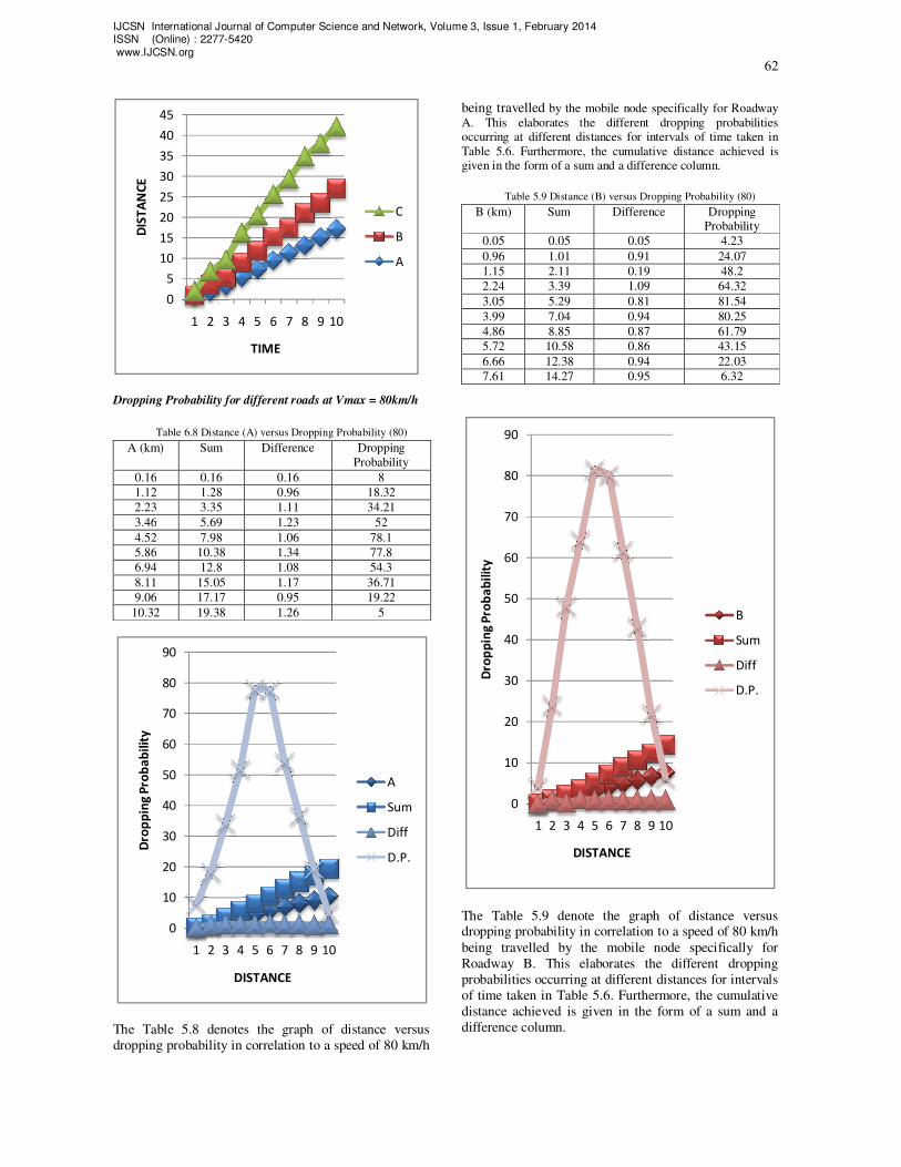
Dropping Probability for different roads at Vmax = 80km/h

Table 6.8 Distance (A) versus Dropping Probability (80)

A (km) Sum Difference Dropping

Probability

0.16 0.16 0.16 8

1.12 1.28 0.96 18.32

2.23 3.35 1.11 34.21

3.46 5.69 1.23 52

4.52 7.98 1.06 78.1

5.86 10.38 1.34 77.8

6.94 12.8 1.08 54.3

8.11 15.05 1.17 36.71

9.06 17.17 0.95 19.22

10.32 19.38 1.26 5

The Table 5.8 denotes the graph of distance versus

dropping probability in correlation to a speed of 80 km/h

being travelled by the mobile node specifically for Roadway

A. This elaborates the different dropping probabilities occurring at different distances for intervals of time taken in

Table 5.6. Furthermore, the cumulative distance achieved is given in the form of a sum and a difference column.

Table 5.9 Distance (B) versus Dropping Probability (80)

B (km) Sum Difference Dropping Probability

0.05 0.05 0.05 4.23

0.96 1.01 0.91 24.07

1.15 2.11 0.19 48.2

2.24 3.39 1.09 64.32

3.05 5.29 0.81 81.54

3.99 7.04 0.94 80.25

4.86 8.85 0.87 61.79

5.72 10.58 0.86 43.15

6.66 12.38 0.94 22.03

7.61 14.27 0.95 6.32

The Table 5.9 denote the graph of distance versus dropping probability in correlation to a speed of 80 km/h

being travelled by the mobile node specifically for

Roadway B. This elaborates the different dropping

probabilities occurring at different distances for intervals

of time taken in Table 5.6. Furthermore, the cumulative

distance achieved is given in the form of a sum and a

difference column.

0

5

10

15

20

25

30

35

40

45

1 2 3 4 5 6 7 8 9 10

DIS

TA

NC

E

TIME

C

B

A

0

10

20

30

40

50

60

70

80

90

1 2 3 4 5 6 7 8 9 10

Dro

pp

ing

Pro

ba

bil

ity

DISTANCE

A

Sum

Diff

D.P.

0

10

20

30

40

50

60

70

80

90

1 2 3 4 5 6 7 8 9 10

Dro

pp

ing

Pro

ba

bil

ity

DISTANCE

B

Sum

Diff

D.P.


63

Table 5.10 Distance (C) versus Dropping Probability (80)

C (km) Sum Difference Dropping Probability

3.36 3.36 3.36 2.21

4.58 7.94 1.22 21.46

6.01 10.59 1.43 50.69

7.85 13.86 1.84 68.23

8.25 16.1 0.4 75.11

9.36 17.61 1.11 77.26

10.27 19.63 0.91 67.14

11.42 21.69 1.15 46.8

13.65 25.07 2.23 23.47

15.02 28.67 1.37 3.65

The Table 5.10 denote the graph of distance versus

dropping probability in correlation to a speed of 80 km/h

being travelled by the mobile node specifically for

Roadway C. This elaborates the different dropping




difference column.

Dropping Probability for different roads at Vmax = 120km/h

Table 5.11 Distance (A) versus Dropping Probability (120)

A (km) Sum Difference Dropping Probability

0.75 0.75 0.75 8

1.86 2.61 1.11 18.32

3.24 5.1 1.38 34.21

5.41 8.65 2.17 52

7.32 12.73 1.91 78.1

9.52 16.84 2.2 77.8

11.28 20.8 1.76 54.3

13.18 24.46 1.9 36.71

15.07 28.25 1.89 19.22

17.11 32.18 2.04 5

The Table 5.11 denote the graph of distance versus

dropping probability in correlation to a speed of 120

km/h being travelled by the mobile node specifically for

Roadway A. This elaborates the different dropping




difference column.

Table 5.12 Distance (B) versus Dropping Probability (120)

B (km) Sum Difference Dropping

Probability

0.18 0.18 0.18 4.23

1.59 1.77 1.41 24.07

2.23 3.82 0.64 48.2

3.48 5.71 1.25 64.32

4.46 7.94 0.98 81.54

5.75 10.21 1.29 80.25

6.12 11.87 0.37 61.79

7.86 13.98 1.74 43.15

8.35 16.21 0.49 22.03

9.92 18.27 1.57 6.32

0

10

20

30

40

50

60

70

80

90

1 3 5 7 9

Dro

pp

ing

Pro

ba

bil

ity

DISTANCE

C

Sum

Diff

D.P.

0

20

40

60

80

100

1 2 3 4 5 6 7 8 9 10

Dro

pp

ing

Pro

ba

bil

ity

DISTANCE

A

Sum

Diff

D.P.

0

10

20

30

40

50

60

70

80

90

1 3 5 7 9

Dro

pp

ing

Pro

ba

bil

ity

DISTANCE

B

Sum

Diff

D.P.


64




Roadway B. This elaborates the different dropping


of time taken in Table 5.7. Furthermore, the cumulative distance achieved is given in the form of a sum and a

difference column.

Table 5.13 Distance (C) versus Dropping Probability (120)

C (km) Sum Difference Dropping Probability

1.01 1.01 1.01 2.21

3.26 4.27 2.25 21.46

4.15 7.41 0.89 50.69

7.31 11.46 3.16 68.23

8.66 15.97 1.35 75.11

10.27 18.93 1.61 77.26

11.89 22.16 1.62 67.14

13.72 25.61 1.83 46.8

14.53 28.25 0.81 23.47

15.02 29.55 0.49 3.65




Roadway C. This elaborates the different dropping



distance achieved is given in the form of a sum and a difference column.

5.6 Inference for Distance

In this paper I have taken into account three types of

roads to give us a brief look at how certain roads affect the speeds at which a node travels which in turn gives

rise to a difference in the times taken by them to reach

their destinations on their respective paths.

A is the first kind of road. I have taken it to be a normal

road meaning it has a little edge here or a little puddle

there but overall it averages out to a flat surface. Thus

the distances travelled in each interval tend to remain

constant or at least have a high degree of similarity. A

perfect example of such a road would be a normal

everyday road being travelled upon by cars, bikes and other vehicles. This road tends to give out a good

estimate of the Dropping Probability for both 80km/h

and 120km/h speeds.

B is the second kind of road. It is mentioned to be a

bumpy one for lack of a better terminology that would

clearly define this road’s aspects. It would rather

resemble a dirt road that has been seldom travelled thus

making a journey through it arduous and painfully slow

as compared to its high paced counterparts. The constant

jolts that are felt will definitely cause a change for the

reception of the signal at a micro level which in turn gives rise to a slightly higher Dropping Probability

value. Examples of roads like this would be the

untrodden ghat roads. Furthermore for roads such as

these there is always a danger of there being a landslide

causing a huge amount of disruption and interference

leading to the signal or call being eventually dropped

due to the fact of the obstacle providing poor reception.

Even if one does manage to reach high speeds, which

actually seems impossible, one may have to give up on

the prospect of maintaining a call unless a very strong

base station is available. Overall the Dropping Probability increases in a steady manner for both cases.

C is the third and last kind of road being a mixture of a

very smooth and a very rough surface. The former

would be similar to a race track and the latter to a village

road in a marsh or swamp conditions. Thus the smooth

surface would offer a higher acceleration growth leading

to a lower Dropping Probability whereas for the rough

wetland surface there would be a lower acceleration

growth causing the Dropping Probability to increase due

to jolts and random movements of the node. Hence in

some places the DP would increase sharply where in

others it would do so at a slower rate.

If we look at all the tables and charts except for the first

two we would notice that there is a sum and a difference

column. These values have either been summed or

accumulated into the upper previous values or they have

been subtracted or differenced from them. This has been

done to properly analyze the distances being covered

and give proper inferences for the Dropping

Probabilities.

0

10

20

30

40

50

60

70

80

90

1 2 3 4 5 6 7 8 9 10

Dro

pp

ing

Pro

ba

bil

ity

DISTANCE

C

Sum

Diff

D.P.


65

6. Conclusion

The proposed Soft-Dual-Handoff scheme aims at

providing high quality data link for the rapid motion

nodes. It has high reliability, which is important for

applications such as subway control, video or audio

transmission. If one link is broken- down, the SDH

switch automatically to single network card mode,

which can earn time for resuming from failure. The SDH

requires only the cooperation of mobile nodes, and AP

needn’t any modification. Therefore, AP can adopt

standard IEEE 802.11 serial products to save

investment.

In fast MSs, a handoff occurs frequently in WLANs due

to their small coverage area. It implies that the frequency

of handoff s will increase especially in WLANs, so a

large number of handoff requests must be handled.

Therefore, the handoff dropping probability is

increasing, and the service quality (e.g., GoS) becomes

worse. On the other hand, the CDMA system is large

enough to accommodate fast MSs, and lower handoff

request rates, thus resulting in lower burden and good

service quality. It is safe to assume that either slow or stationary MSs transmit more data and that fast moving

stations communicate at lower data rates. Therefore,

according to the MS speed, the load balancing handoff

between WLAN and CDMA results in good service

quality and the avoidance of unnecessary handoff s. Our

proposed methods adopt the mobility management

concept through the MS speed cost function to minimize

the GoS.

References

[1] John Y. Kim and Gordon L. Stuber, “CDMA Soft

Handoff Analysis in the Presence of Power Control

Error & Shadowing Correlation”, IEEE Transactions on Wireless Communications, Vol. 1, No. 2, pp. 245-255, April 2002.

[2] Bechir Hamdaoui and Parameswaran Ramanathan, “A Network Layer Soft Handoff Approach for Mobile

Wireless IP-Based Systems”, IEEE Journal on Selected Areas in Communications, Vol. 22, No. 4, pp. 630-642, May 2004.

[3] Qian Hong-Yan, Chen Bing & Qin Xiao-Lin, “A Dual-Soft-Handoff Scheme for Fast Seamless

Roaming in WLAN”, 2010 Second International Conference on Networks Security, Wireless

Communications & Trusted Computing, pp. 97-100,

2010. [4] John Y. Kim, Gordon L. Stuber, Ian F. Akyildiz &

Boo-Young Chan, “Soft Handoff Analysis of Hierarchical CDMA Cellular Systems”, IEEE

Transactions on Vehicular Technology, Vol. 54, No. 3, pp. 1122-1134, May 2005.

[5] Sung Jin Hong & I-Tai Lu, “Effect of Various

Threshold Settings on Soft Handoff Performance in Various Propagation Environments”, pp. 2945-2949,

VTC 2000. [6] Yali Qin, Xibing Xu, Ming Zhao & Yan Yao, “Effect

of User Mobility on Soft Handoff Performance in

Cellular Communication”, Proceeding of IEEE TENCON’02, pp. 956-959, 2002.

[7] Rajat Prakash and Venugopal V. Veeravalli, “Locally Optimal Soft Handoff Algorithms”, IEEE

Transactions on Vehicular Technology Vol. 52, No. 2,

pp. 347-356, March 2003.

Mr. Sayem Patni received his M. E. Degree in Electronics and Telecommunication from Terna College of Engineering, Mumbai University in 2013 and his B. E. Degree in Electronics and Telecommunication from Xavier Institute of Engineering, Mumbai University in 2010. He has worked at Xavier Institute of Engineering as a Lecturer for one year from July 2011 to June 2012 and has been continually working for the CMAT Exams as an IT Administrator. He has passed GRE and TOEFL with a score of 1390 and 106 respectively. He has published and presented 12 papers in International Conferences and Journals. He has attended various STTP programs ranging from Wireless to Microwaves to Software Enrichment. Currently he is working on the development of Dual Soft Handoff and its applications.

Evaluation of Dual Soft Handoff in a Seamless Roaming...

Documents

Transcript of Evaluation of Dual Soft Handoff in a Seamless Roaming...