EVALUATION OF DESIGN TOOLS FOR THE MICRO-RAM AIR …

EVALUATION OF DESIGN TOOLS FOR THE MICRO-RAM AIR TURBINE

A Thesis

presented to

the Faculty of California Polytechnic State University,

San Luis Obispo

In Partial Fulfillment

of the Requirements for the Degree

Master of Science in Mechanical Engineering

by

Victor Fidel Villa

April 2015

ii

© 2015

Victor Fidel Villa

ALL RIGHTS RESERVED

iii

COMMITTEE MEMBERSHIP

TITLE: Evaluation of Design Tools for the Micro-Ram Air

Turbine

AUTHOR: Victor Fidel Villa

DATE SUBMITTED: April 2015

COMMITTEE CHAIR: Dr. Russell Westphal, Professor

Mechanical Engineering Department

COMMITTEE MEMBER: Dr. William R. Murray, Professor

Mechanical Engineering Department

COMMITTEE MEMBER: Dr. Rob McDonald, Associate Professor

Aerospace Engineering Department

iv

ABSTRACT

Evaluation of Design Tools for the Micro-Ram Air Turbine

Victor Fidel Villa

The development and evaluation of the design of a Micro-Ram Air Turbine (µRAT), a

device being developed to provide power for an autonomous boundary layer

measurement system, has been undertaken. The design tools consist of a rotor model and

a generator model. The primary focus was on developing and evaluating the generator

model for the prediction of generator brake power and output electrical power with and

without rectification as a function of shaft speed and electrical load, with only basic

manufacturer specifications given as inputs. A series of motored generator evaluation test

were conducted at speeds ranging from 9,000 to 25,000 rpm for loads varying between 1

and 3.02 Ohms with output power of up to 80 Watts. Results demonstrated that predicted

generated power was at or below 3% error when compared to measured results with

about 1% uncertainty. A rotor model was also developed using basic blade element

theory. This model neglected induced flow effects and was therefore expected to over

predict rotor torque and power. A second rotor model that includes induced flow effects,

the open source program X-Rotor, was also used to predict rotor power and for

comparison to the blade element rotor model results. Both rotor models were evaluated

through wind tunnel validation tests conducted on a turbine generator with two different

3.25 in diameter rotors, rotor-1 (untwisted blades) and rotor-2 (twisted blades). Wind

tunnel validation test airspeeds varied between 71-110 mph with electrical loads ranging

from 1-20 ohms. Results indicated power predictions to be 50-75% higher for the blade

element model and 20-30% for X-Rotor results. The blade element rotor model was

modified by applying the Prandtl tip-loss factor to approximately account for the induced

flow effects; this addition brought predictions much closer to X-Rotor results. Based on

the motor-driven generator test results, it is believed that most of the discrepancy in

baseline rotor/generator validation test between predicted and observed power generated

is due to inaccuracy in the rotor performance modeling with likely contributors to error

being induced flow effects, crude section lift/drag modeling, and aero-elastic

deformation. It is concluded that the proposed generator model is sufficient although

direct torque measurements may be desired and further development of the µRAT design

tools should focus on an improved rotor performance model.

Keywords: Micro-RAT, Blade Element Model, Generator Model

v

ACKNOWLEDGMENTS

A special thanks to the Northrop Grumman Corporation for their support of the BLDS.

I would like to extend a sincere thank you to Dr. Russell Westphal for his unfaltering

energy and enthusiasm that inspires excellence and the desire to pursue and overcome

new challenges. Your exemplary leadership, motivation, and work ethic are things that I

will carry with me in everything I do.

A big thanks to the BLDS team! You all have amazing talents! It has been a pleasure

working with you all and hope to work with you all in the future.

Thanks to my family for their continued love and support. Specifically my parents, Fidel

and Rosa Villa; everything I have achieved and will achieve is a result of your loving

support, sacrifice and hard work.

I would like to add a special thanks to my high school instructor and mentor, Mr. John

Vogt who steered me towards pursuing engineering. In my pursuit for a career in

aviation, he convinced me to look into engineering when he told me, “If you want to

learn how to fly a plane you first have to learn why they fall out of the sky”. Thank you!

vi

TABLE OF CONTENTS

LIST OF TABLES viii

LIST OF FIGURES x

NOMENCLATURE xv

1. Introduction 1

2. Generator Model 20

2.1 Generator Performance Parameters ......................................................................... 21

2.1.1 Internal Resistance and Impedance ............................................................ 21

2.1.2 No Load Current ........................................................................................ 23

2.1.3 Torque Constant ......................................................................................... 24

2.1.4 Speed Constant .......................................................................................... 24

2.1.5 Cogging Torque ......................................................................................... 24

2.2 Motor Model ............................................................................................................ 26

2.3 Generator Electrical Model ...................................................................................... 30

2.4 Power Rectification .................................................................................................. 36

2.5 Generator/Motor Model Comparison ...................................................................... 41

2.6 Generator Model Evaluation (Validation) Testing .................................................. 43

3. Rotor Model 57

3.1 Actuator Disk Theory .............................................................................................. 58

3.2 Blade Element Theory ............................................................................................. 64

3.3 X-Rotor .................................................................................................................... 76

4. Rotor/Generator Matching 83

5. Baseline Rotor/Generator Validation Test 96

5.1 Apparatus Design and Development ....................................................................... 96

5.1.1 Rotor ......................................................................................................... 97

5.1.2 Rotor/Generator Adapter ........................................................................... 99

5.1.3 Generator Housing ................................................................................... 100

vii

5.1.4 Test Stand ................................................................................................ 101

5.2 Validation Test Results .......................................................................................... 102

5.3 Discussion .............................................................................................................. 108

5.4 Rotor Model Tip Loss Corrections ........................................................................ 109

6. Conclusion and Recommendations 116

References 121

Appendices

Appendix A. Rotor Model Matlab 125

Appendix B. Generator Model Matlab 130

B.1 Generator Model Efficiency Contour Charts ............................................................ 132

Appendix C. Motor Model Matlab 135

C. 1 Motor Model Efficiency Contour Charts Matlab .................................................... 136

Appendix D. Generator Model Evalutaion Test Results 138

Appendix E. Blade Element Rotor Model Peak Power Sectional Results 146

viii

LIST OF TABLES

Table 1. BLDS Power Consumption @ -55° C [1] ............................................................ 3

Table 2. Selection of Generator Type Decision Matrix [7] ................................................ 7

Table 3. Selection of Wind Turbine Type Decision Matrix [7] ........................................ 13

Table 4. Motor/Generator Equation Comparison ............................................................. 42

Table 5. Generator Kv Verification Results ..................................................................... 45

Table 6. Internal Resistance Measurement Results .......................................................... 46

Table 7. Generator Parameter Verification ....................................................................... 47

Table 8. Generator Model Test Results at 3.02 Ohms ...................................................... 49

Table 9. Motor Parameter Verification [Ammo BLDC (part# 35-56-1800kv)] ............... 51

Table 10. DC Motor Shaft Torque Calculation ................................................................ 52

Table 11. Generator Shaft Torque Calculation ................................................................. 53

Table 12. Motor/Generator Shaft Torque ......................................................................... 54

Table 13. Motor to Generator Terminal Power Calculation ............................................. 55

Table 14. Motor to Generator Model Calculated Terminal Power Compared

to Actual .................................................................................................... 56

Table 15. Rotor Geometric Parameters ............................................................................. 69

Table 16. Rotor-Generator Performance at Maximum Rotor Power Operating

Point for Rotor-1 ....................................................................................... 88

Table 17. Rotor-Generator Performance at Max Rotor Power Operating Point

for Rotor-2 ................................................................................................ 90

Table 18. Generator A and B Manufacturer Specifications .............................................. 91

Table 19. Generator-B Efficiency at Maximum Rotor-1 Power Operating

Point .......................................................................................................... 94

Table 20. Differential Pressures and Pressure Coefficients across the Wind

Tunnel Nozzle ......................................................................................... 103

Table 21. Airspeed Calculation for Rotor-1 and Rotor-2 Test ....................................... 104

Table 22. Generator Evaluation Test Results (RL=1.04) (Maxon #386677) ................. 138


ix







Table 30. Rotor-1 Blade Element Rotor Model Sectional Results at Peak

Power @ Sea Level, 110 mph and 21,000 RPM .................................... 146

Table 31. Rotor-2 Blade Element Rotor Model Sectional Results at Peak

Power @ Sea Level, 110 mph and 21,000 RPM .................................... 147

x

LIST OF FIGURES

Figure 1. Preston tube data system (PTDS) [1] .................................................................. 2

Figure 2. Boundary Layer data system (BLDS) [1] ............................................................ 2

Figure 3. Basic Electric Machines [3] ................................................................................. 4

Figure 4. Brushed Motor/Generator Commutator and Brushes [5] [6] .............................. 5

Figure 5. Team AeroRAT Generator Test Schematic [7] ................................................... 8

Figure 6. Team AeroRAT Generator Test Setup [7] .......................................................... 8

Figure 7. Team AeroRAT Proof-of-Concept Test Results [7] ........................................... 9

Figure 8. Equivalent Circuit of a DC Motor [8] ............................................................... 10

Figure 9. Motor and Propeller Parameters at Specific Flight Speed and Motor

Voltage [8] ................................................................................................ 11

Figure 10. Types of Wind Turbines [7] ............................................................................ 12

Figure 11. Wind Turbine Actuator Disk [13] ................................................................... 14

Figure 12. Betz Limit at Different Altitudes for Varying Airspeed ................................. 15

Figure 13. Team AeroRAT Proof-of-Concept Wind Tunnel Test Results [7] ................. 17

Figure 14. Micro-RAT Design Task Chart ....................................................................... 19

Figure 15. BLDC Motor/Generator Stator and Rotor [17] ............................................... 25

Figure 16. Cogging Torque at Different Rotor Positions [16] .......................................... 25

Figure 17. Prime Mover DC Motor Model Electrical schematic [8] ................................ 27

Figure 18. Maxon Motor Manufacturer Performance Parameters for BLDC

Motor #386677 [14] [18] .......................................................................... 28

Figure 19. Motor Model Predicted Torque and Brake Power .......................................... 29

Figure 20. Motor Model Predicted Efficiency .................................................................. 29

Figure 21. Motor Model Efficiency Contour Chart .......................................................... 30

Figure 22. Generator Model Electrical schematic [8] ....................................................... 31

Figure 23. Generator Model Predicted Torque and Shaft Power at 5 Ohms .................... 33

Figure 24.Generator Model Predicted Efficiency at 5 Ohms ........................................... 34

Figure 25. Brake Torque and Power for different Electrical Loads ................................. 35

Figure 26. Generator Model Efficiency Contour Chart .................................................... 35

xi

Figure 27. Diode Current - Voltage relationship [19] ....................................................... 36

Figure 28. Half Wave Rectification [20] .......................................................................... 37

Figure 29. Full Wave Rectification [20] ........................................................................... 37

Figure 30. Voltage rectification using 3-phase bridge rectifier [21] ................................ 38

Figure 31. Current - Voltage per Diode in IXYS FUO 22 Three Phase

Rectifier Bridge [21] ................................................................................. 38

Figure 32. Generator Model Electrical schematic [8] [9] ................................................. 39

Figure 33. Generator Model Predicted Torque and Shaft Power [5 Ohms

(Rectified)] ................................................................................................ 41

Figure 34. Generator Model Predicted Efficiency at 5 Ohms (Rectified) ........................ 41

Figure 35. Generator Kv Test Schematic .......................................................................... 43

Figure 36. Generator Kv Test Setup ................................................................................. 44

Figure 37. Electrical Schematic of Generator Internal Resistance

Measurement ............................................................................................. 46

Figure 38. Generator Test Schematic ................................................................................ 48

Figure 39. Generator Test Setup ....................................................................................... 48

Figure 40. Generator Model Test Results at 3.02 Ohms................................................... 49

Figure 41. DC Motor No-Load Current ............................................................................ 51

Figure 42. Torque Verification diagram ........................................................................... 53

Figure 43. Motor and Generator Model Predicted Shaft Torque ...................................... 54

Figure 44. Motor to Generator Model Validation Test Diagram ...................................... 55

Figure 45. Turbine Actuator Disk ..................................................................................... 58

Figure 46. Power and Thrust Coefficients ........................................................................ 62

Figure 47. Power Curve for a 3.25 in. Diameter Rotor ..................................................... 62

Figure 48. Actuator Disk Power Extracted for Different Axial Velocities at

Varying Axial Induction Factors. (Dotted Line Represents

Betz Limit) ................................................................................................ 63

Figure 49. Schematic of Rotor Blade Partitioned into Blade Elements [13] .................... 64

Figure 50. Blade Velocity and Force Breakdown [12] ..................................................... 65

Figure 51. Blade Element Model Iteration Diagram ........................................................ 68

Figure 52. Baseline Rotors 1 & 2...................................................................................... 69

xii

Figure 53. Selected Rotor Blade Airfoil (NACA 2412) ................................................... 70

Figure 54. QBlade GUI for Analyzing Airfoil CL and CD [23] [22] ............................... 71

Figure 55. Montgomery Extrapolated NACA 2412 Lift and Drag curves at

Re:80,000;Using QBlade Extrapolation Module [23] [22]....................... 72

Figure 56. Blending Function for Combining Potential and Thin Plate Flow

for Montgomery Extrapolation Method [25] ............................................ 73

Figure 57. Inverted NACA 2412 [23] [22] ....................................................................... 74

Figure 58. Blade Element Model Power and Torque Predictions for Rotor-1

Model for Airspeed of 110 mph................................................................ 75

Figure 59. Blade Element Model Power and Torque Predictions for Rotor-2

Model for Airspeed of 110 mph................................................................ 76

Figure 60. XROTOR Startup Window [22] ...................................................................... 77

Figure 61. X-Rotor Aerodynamic Submenu [22] ............................................................. 78

Figure 62. XROTOR Aerodynamic Section Editting Submenu [22] ............................... 78

Figure 63. Straight and Twisted Blade Geometry Created in XROTOR [22] .................. 79

Figure 64. X-Rotor Rotor Analysis Results [22] .............................................................. 80

Figure 65. Rotor 1 (straight blades) Predicted Power @ 110 mph (sea level) ................. 81

Figure 66. Rotor 1 (straight blades) Predicted Torque @ 110 mph (sea level) ................ 81

Figure 67. Rotor 2 (twisted blades) Predicted Power @ 110 mph (sea level) .................. 82

Figure 68. Rotor 2 (twisted blades) Predicted Torque @ 110 mph (sea level)................. 82

Figure 69. Rotor/Generator Matching Process ................................................................. 84

Figure 70. Maxon (#386677) Generator Efficiency Contour Map ................................... 85

Figure 71. Maxon (#386677) Generator Brake Torque and Power for

Terminal Loads 1-20 Ohms ...................................................................... 85

Figure 72. Rotor-1 Brake Power Plotted onto Generator Efficiency Contour

[Generator: Maxon #386677]; [ @ sealevel, 110 mph, Betz

Limit=230 Watts] ...................................................................................... 86

Figure 73. Rotor 1 Brake Torque and Power Curves Overlaid Generator

Brake Torque and Power plots fort varying Electrical Loads of

1-20 Ohms ................................................................................................. 87

Figure 74. Rotor-2 Generator Efficiency Contour Plot .................................................... 88

xiii

Figure 75. Rotor Brake Torque and Power Curves Overlaid Generator Brake

Torque and Power plots fort varying Electrical Loads of 1-20

Ohms ......................................................................................................... 89

Figure 76. Generator-B Manufacturer Specifications [Maxon #386678] [18] ................ 91

Figure 77. Rotor-1 & Generator B Efficiency Contour .................................................... 92

Figure 78. Rotor-1 Brake Torque and Power Curves Overlaid Generator-B

Brake Torque and Power plots fort varying Electrical Loads of

1-20 Ohms ................................................................................................. 93

Figure 79. Turbine Generator Assembly .......................................................................... 97

Figure 80. Rotor/Generator Adapter ................................................................................. 99

Figure 81. Front part of generator housing ..................................................................... 100

Figure 82. Aft part of generator housing [26] ................................................................. 100

Figure 83. Test Stand Attached to Bottom Wind Tunnel Plate [26] ............................... 101

Figure 84. Turbine Generator Mounted on Test Stand [26] ........................................... 101

Figure 85. Turbine Generator Validation Test Schematic [26] ...................................... 102

Figure 86. Rotor/Generator Test Setup ........................................................................... 103

Figure 87. Rotor-1 Power @ 49.05m/s compared to model predictions ........................ 105

Figure 88. Rotor 2 Power @ 49.05m/s compared to model predictions ......................... 105



Figure 91. Rotor-1 Power @ 32.79 m/s compared to model predictions ....................... 107


Figure 93. Prandtl Tip Loss Factor (Fp) as a Function of Normalized Radius ............... 110

Figure 94. Sectional Torque without Tip Loss Factor .................................................... 111

Figure 95. Sectional Torque with Tip Loss Factor ......................................................... 111


Figure 97. Rotor-2 Power @ 49.05m/s Compared to Model Predictions ....................... 113



Figure 100. Rotor-1 Power @ 32.79 m/s Compared to Model Predictions .................... 115

Figure 101. Rotor-2 Power @ 32.79m/s Compared to Model Predictions ..................... 115

xiv

Figure 102. Generator Evaluation Test Results (RL=1.04) (Maxon #386677) .............. 138








xv

NOMENCLATURE

IO = No-load current, amps

Ri = Internal resistance, ohms

RL = Terminal electrical load, ohms

L = Inductance, henry

KV = Speed constant, rpm/volt

KT = Torque constant, N-m/amp

P = Power, watts

Va = Armature Voltage, volts

Vr = Rectified terminal voltage, volts

VDO = Rectifier forward voltage drop, volts

Pbrake = Power at the shaft, watts

Q = Torque, lbf-ft

η = Efficiency

RPM = Revolutions per minute

V∞ = Freestream airspeed, ft/s

VO = Axial airspeed at rotor face, ft/s

V1 = Relative airspeed, ft/s

φ = Relative velocity angle, °

α = Angle of attack, °

ΔT = Sectional Thrust, lbf

ΔQ = Sectional Torque, lbf-ft

l = Sectional Lift, lbf

d = Sectional Drag, lbf

1

1. INTRODUCTION

The development of a Micro Ram Air Turbine (µRAT) system is being investigated

to provide power to a heating element that will eliminate sensor drop out due to cold

temperatures on the Boundary Layer Data System (BLDS) during high altitude flights. In

addition, a µRAT could be used to augment or replace the BLDS battery for extended

operation. This thesis project builds on previous proof-of-concept work with the aim of

developing a set of design tools to intelligently design the µRAT turbine/generator for

specific operating conditions and particularly to match a turbine rotor to an appropriate

generator. The µRAT design tools consist of turbine rotor and generator models; the

latter is the primary focus of the current work. The generator will undergo a series of

motored generator tests followed by wind tunnel tests for the fully assembled turbine

generator. Results are then used to evaluate the design tools, and particularly to improve

and validate the generator model.

The Boundary Layer Data System (BLDS) along with the Preston Tube Data

System (PTDS) are Northrop Grumman Corp. sponsored devices developed by Dr.

Russell Westphal and the BLDS team for the purpose of measuring in-flight boundary

layer and airflow properties. These devices are standalone, battery powered, flight rated

devices that can be non-intrusively attached to any aircraft or surface and operate

autonomously without having to task an operator for data collection. Both of these

systems are capable of measuring absolute static pressure, temperature and average skin

friction. The BLDS can additionally measure mean boundary layer velocity profile with a

Pitot tube that is mounted onto a motorized stage. The PTDS measures three pressures

2

simultaneously, these include free-stream dynamic pressure using a Pitot tube, local

surface static pressure using the Sproston-Goskel probe, and skin friction using the

Preston tube [1].

Figure 1. Preston Tube Data

System (PTDS) [1]

Figure 2. Boundary Layer Data

System (BLDS) [1]

Both systems share similar basic components such as: the microcontroller, data

storage, battery, pressure sensors and pressure probes. The battery pack consist of 4 AA

sized Lithium Sulfur Dioxide (LiSO2) batteries that provide up to 1000mAhr and 12 V at

20° C. Components such as the microcontroller and sensors are not rated to operate at

temperatures below -20° C, however, test results have shown continued operation down

to and below -55° C. Battery and sensor performance have been observed to rapidly

diminish at temperatures below -55° C. Typically at theses temperatures the battery

output diminishes to 250 mAHr and 10 V and sensors are more likely to fail [1]. To

approximate the maximum power required to power the BLDS, Table 1 reflects the

power requirements at temperatures of -55° C, which impose higher power requirements

than at higher temperatures. The higher power requirements are mainly due to the higher

current draw from the stage, which is dependent on temperature and is higher at lower

temperatures – all other parts draw a fixed current, independent of temperature. Our

3

approximation concludes that no more than a couple of watts are required to power all

components of the BLDS at its coldest operating temperature. It should also be noted that

the BLDS conserves power consumption by going to sleep mode, which turns off all

components with exception of the micro controller when data is not being collected.

Table 1. BLDS Power Consumption @ -55° C [1]

Current Draw (mA) 4 x LiSO2

Voltage @ -55 C

Approx. Power

Required (Watts)

Pressure Sensor 24 (3 @ 8 each) 10 0.24

Temp. Sensor (x1) 1 10 0.01

Stage Motor 25-100+ 10 1

Micro Controller 4 (sleep), 14 (operation) 10 0.14

Total: 1.39 max

Previous work investigated the possibility of eliminating sensor dropout through

insulation and self-heating. A study conducted by Htet htet Oo [2] investigated the

possibility of maintaining a 1-degree temperature difference between ambient air and

internal temperatures. In this study, a BLDS satellite was modeled with a prototype

circuit board within a “sandwich” of insulation. Within the insulation, a heating element

simulated the generated heat, typical of a BLDS satellite circuit board [2]. Estimates

based on this study indicate an average heat dissipation per Kelvin of 46 mW/K.. Based

on this estimate it is feasible to gain a few degrees of temperature through the use of self-

heating and insulation, however a more substantial increase in internal temperatures can

be achieved through providing additional heat. These results further demonstrate how an

insulated BLDS would require modest power for heating. For an insulated BLDS satellite

a 10° internal temperature rise would require an estimated 0.5 watts in addition to what is

required to power the BLDS, as outlined in Table 1. A total of less than 2 watts,

4

maximum, would be required to power the BLDS and provide sufficient heat for an

internal temperature rise of 10°. In the development of the µRAT for the purpose of

heating the BLDS, it is the generator that directly supplies this power to the heating

element. A thorough understanding of the generator will enable the optimization and

proper matching of rotor performance and overall system efficiency for a required

heating element.

Electric generators along with motors are electric machines that convert

mechanical power to electrical energy or conversely convert electrical energy to

mechanical power. Basic laws such as Faraday’s law of electromagnetic induction and

Lorentz’s force law explain the fundamental working principles of typical electrical

motors and generators; this is illustrated below in Figure 3. The motoring application can

be understood from the Lorentz Force Law, which explains how a current passing

through a conductor that is freely suspended within a fixed magnetic field will create a

force, resulting in the motion of the conductor through the magnetic field [3] [4].

Figure 3. Basic Electric Machines [3]

The generator application is understood through Faraday’s explanation of how a

moving conductor through a magnetic field or moving a magnetic field relative to a

conductor will induce a current through the conductor. Brushed generators and motors

5

rely on Faraday’s law and Lorentz’s force law. These type of electric machines, shown in

Figure 4, run current to the rotating shaft or “coil” through carbon brushes that make

contact with a commutator that rotates with the shaft.

Figure 4. Brushed Motor/Generator Commutator and Brushes [5] [6]

DC brushed machines have advantages that include low cost, high reliability, and

simplicity that is, they do not require a controller to operate. Some disadvantages include

high maintenance, low life span, and low efficiencies. Many of the disadvantages are due

to the carbon brushes and rotating commutator required to make moving electrical

contact with the shaft. These components are responsible for additional frictional losses

and tend to wear rapidly under continued operation.

While DC brushless electrical machines depend on the Lorentz force, it also takes

advantage of an additional method of motor power. This motoring power comes from the

reluctance torque; reluctance torque takes advantage of the repulsive and attractive force

that is exerted on a magnet or any magnetic material when it is placed in the field of

another magnet. The motoring motion is established through the pulsing and switching of

stator poles in order to rotate the magnetic field; the magnetic field then brings the

6

magnet along with it as it rotates. For this phenomenon to be practical, one of the

magnets must be an electro-magnet. This will ensure control of the magnetic field

necessary for continued motion. BLDC motors rely on a speed controller to manage the

pulsing a switching of stator poles in order to drive the motor. Running these machines

backwards as generators produces AC voltages and currents requiring a rectifier if it is

desired to convert AC power to DC. Although BLDC machines can alternatively be run

as an AC generator, it is most common to find these machines sold as motors with

manufacturers providing performance charts for the motoring application only. This

prompts the need to develop a generator model that can characterize the performance of a

generator using performance parameters that are typically provided for the motoring

application.

In previous generator proof-of concept work conducted by the AeroRAT senior

design group [7], the type of generator was determined and the need to develop a method

to predict and match rotor performance with an off-the-shelf generator was identified.

Initial selection of the type of candidate generator was based on efficiency, cost, size and

weight. Rotational speed ranges and maintenance requirements were also taken into

account. Table 2 shows the decision matrix used in the selection of the brushless DC

motor as the candidate generator type [7].

7

Table 2. Selection of Generator Type Decision Matrix [7]

Brushless DC motors proved to be more practical for the application of a turbine

generator in that they have reduced maintenance, higher power per unit volume, higher

efficiencies due to not having the wear and mechanical power losses imposed by the

contact of the brushes with the commutator. Additionally, previous experience using

BLDC motors to drive the BLDS stage in flight has proven their successful operability at

low temperatures. Referencing Table 2 it can be seen that team AeroRAT placed most of

the decision weight on the efficiency parameter, which is based off motoring data.

Although these efficiencies were based on motoring efficiencies, these values do provide

a rough estimate of the generator efficiencies.

Upon selecting the BLDC motor as the type of generator, Team AeroRat

conducted generator proof-of-concept test. The test schematic in Figure 5 shows the test

setup with generator lead wires going to a rectifier, where the generated AC current is

converted to DC current. Current then flows through a resistor load bank where terminal

current and voltage are measured.

8

Figure 5. Team AeroRAT Generator Test Schematic [7]

The physical test set up is shown in Figure 6; here we can see that an air powered die

grinder is used as the prime mover to the generator. The die grinder rotates the generator

through a shaft coupler. The three generator lead wires are connected to the rectifier,

which connects to the electrical load as shown. Two multimeters are shown: one is

connected in parallel to measure voltage, and the other in series with the load to measure

current.

Figure 6. Team AeroRAT Generator Test Setup [7]

For the test, terminal power was measured as the die grinder drove the generator through

various rotational speeds with two different loads at the terminal; 12.7 ohms and 10.1

ohms. These results are shown below in Figure 7.

9

Figure 7. Team AeroRAT Proof-of-Concept Test Results [7]

While the feasibility of producing power by rotating the generator was proved, an

optimum operating point for the generator was not determined. Questions such as: What

is the minimum shaft torque required of the blades to turn the generator shaft?, or How

much torque for a given load do the blades need to produce in order to drive the generator

to a speed of optimum efficiency?, were still left unanswered. Although motor data

provides a crude approximation to generator performance, it is important to understand

that power losses are applied differently in a generator and if converting generated AC

power to DC power, rectifier losses also need to be accounted for. In order to efficiently

generate power, a method for predicting generator performance and matching a generator

to the performance of a rotor is necessary [7].

As mentioned before, typically DC brushless machines are sold as motors with

specifications only detailing the motoring applications. In search for a published

generator model suitable for our application, an exact match was not found however,

10

Drela’s explanation of a 3-constant DC motor model [8] along with turbine generator

work done by Wood, D. [9] was of particular interest. The 3-constant DC motor model

explained by Drela implements established electro-mechanics to match a basic DC

Brushless motor to a rotor blade. Wood gives details on different generator electrical

schematics that can be modified for our particular application. Below in Figure 8, a basic

electro-mechanical schematic from Drela’s model details how the DC current induces

torque at the rotor shaft.

Figure 8. Equivalent Circuit of a DC Motor [8]

Although this models the motoring application of an electric machine as it is matched to a

propeller, it is useful in understanding and establishing an approach to modeling a

generator that is to be matched to a turbine. Figure 9 displays the method in which a

propeller is matched to a motor using Drela’s model. Here the schematic of Figure 8 is

used to establish equations to model the motors torque and efficiency as it varies with

RPM. Motor torque and efficiency are then plotted along with propeller torque and thrust

parameters. One can then match the propeller operating points with the motor

performance as seen with the vertical dotted line in Figure 9 [8].

11

Figure 9. Motor and Propeller Parameters at Specific Flight Speed and Motor

Voltage [8]

The motor/propeller matching approach used in Drela’s motor model is used in

establishing a method to optimally match a rotor to a generator and in effectively

predicting performance. For the generator model, an electrical schematic similar to that of

Figure 8 is developed. The electrical model of the generator differs from that of the motor

in that current will flow in the opposite direction and will reflect additional losses

incurred by the generator and rectifier. To match the generator with a rotor, rotor

performance predictions are calculated and matched with generator torque and efficiency

plots. One possible criteria for matching is when rotor peak power is at the same

operating point as generator max-efficiency. Rotor performance predictions will be

developed using methods similar to those previously employed by team AeroRAT [7]

[8].

12

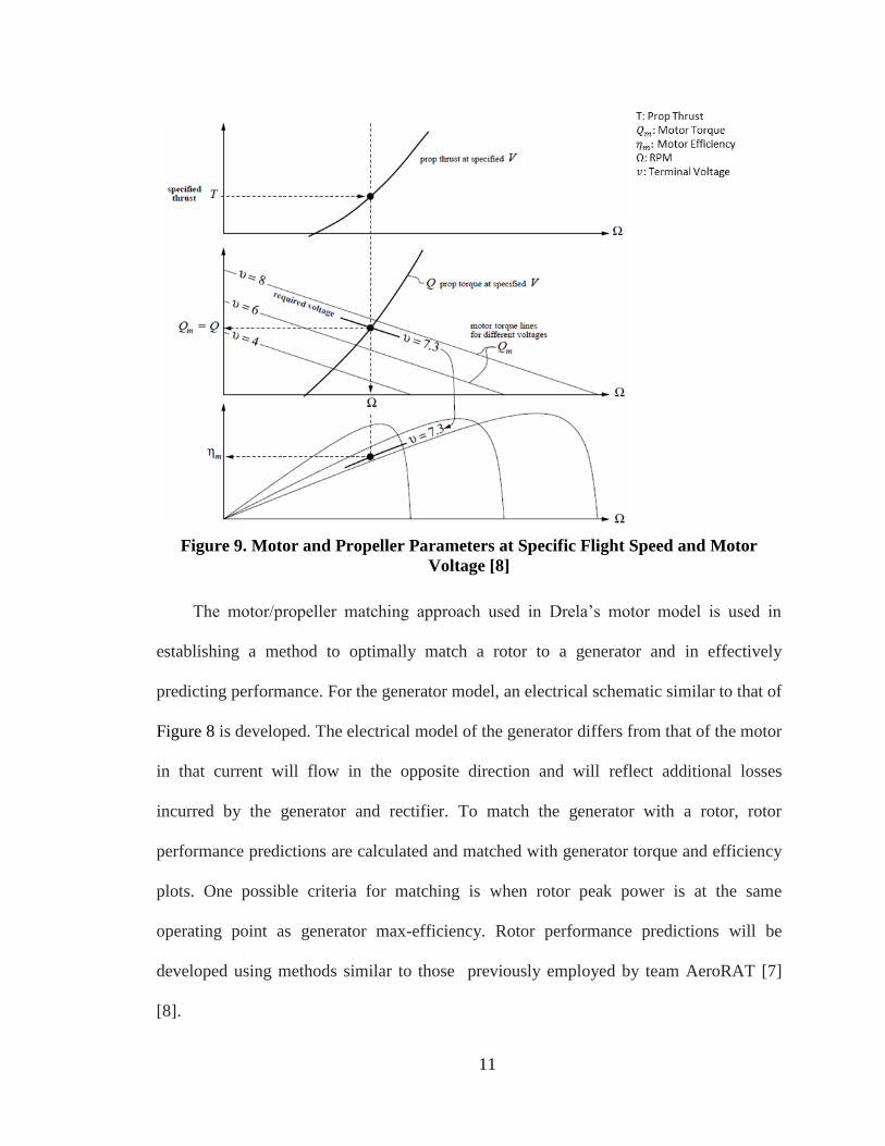
Previous rotor blade design work entailed selecting the blade type, conducting 1st

order calculations to determine rotor sizing, manufacturing, and performing proof of

concept test. In selecting the blade type, different blade concepts such as the ones shown

in Figure 10 were considered by team AeroRAT. These concepts included Axial,

Vertical, Screw, and Paddle Wheel.

Figure 10. Types of Wind Turbines [7]

Vertical axis type of turbines tend to produce cyclical stress and torque ripples resulting

in low reliability and high maintenance. Some variations of vertical axis turbines and

paddle wheel type are also considered drag type turbines and generally are less efficient

then axial turbines. Unlike vertical axis and drag type turbines, axial turbines produce

power throughout the entire rotation from each blade. Vertical axis turbines require the

blade to backtrack against the direction of airflow resulting in lower efficiencies. For the

reasons mentioned above and for the reasons outlined in Table 3, team AeroRAT selected

the axial turbine as the best fit for the application of providing power to a heating element

for the BLDS. To be consistent with previous work, the horizontal axis wind turbine was

selected for this work [10] [7].

13

Table 3. Selection of Wind Turbine Type Decision Matrix [7]

Team AeroRAT [7] additionally conducted first order calculations to size and

determine blade geometry of the rotor. Actuator disk theory was applied in determining

the rotor sizing. This analysis is based on 1-D momentum theory and represents the

turbine as a disc that is infinitely thin uniformly loaded throughout the rotor area. It

assumes a homogenous, inviscid, incompressible, steady flow. Static pressures far

upstream and downstream of the rotor are assumed to be equal to the static ambient

pressure. Figure 11 below illustrates the actuator disc model for a turbine. In the analysis,

Bernoulli’s equation and Newton’s 2nd Law (momentum) are applied to 3 different

control volumes, from station 1-4, 1-2, and 3-4. The velocities represented by U are

assumed uniform across each station [11] [12] [13].

14

Figure 11. Wind Turbine Actuator Disk [13]

Through actuator disk analysis, maximum theoretical power extracted known as the Betz

limit is determined. The Betz Limit states that no bare rotor turbine can extract more than

16/27 (59.26%) of the kinetic energy in the free-stream air flowing through the rotor

swept area [13] [11]. This model is highly idealized, typically commercial turbines only

achieve up to 50% -75% of the Betz Limit. Figure 12 below displays the calculated Betz

limit values in watts per swept area for varying airspeeds at different altitudes. At sea

level, Figure 12 shows the Betz limit ranging from 6.63 watts/in^2 at 100 ft/s to 828.9

watts/in^2 at 500 ft/s [13] [11] [12].

𝐶𝑃 =𝑃𝑒𝑥𝑡𝑟𝑎𝑐𝑡𝑒𝑑𝑃𝑎𝑣𝑎𝑖𝑙𝑎𝑏𝑙𝑒

=16

27 (1)

15

Figure 12. Betz Limit at Different Altitudes for Varying Airspeed

A blade element analysis was also conducted in order to get a better idea of what

type of blade geometry would be required to produce 50 Watts at a target design point of

30,000 ft and airspeed of 400 ft/s. Classic Glauert Blade Element Analysis [11] is a

simple, 2-D, iterative method of predicting performance of a rotor and optimizing

geometric parameters such as blade angle, chord, and twist distribution. It involves the

partitioning of rotor blades into independent sections along the length of the blade. At

each section, thrust and torque are calculated through a force balance that is conducted

using 2-D airfoil lift and drag coefficient data. Sectional thrust and torque values can then

be summed up in order to predict the performance of the entire rotor. This analysis is

limited to 2-D, incompressible flow and does not take into account induced flow effects.

As such, it can only provide a rough approximation of rotor performance [13] [11] [12].

100 150 200 250 300 350 400 450 5000

100

200

300

400

500

600

700

800

900

Velocity (ft/s)

Pow

er

Extr

acte

d p

er

Square

Are

a [

Watt

s/in

2]

Betz Limit

sea level

15000 [ft]

30000 [ft]

45000 [ft]

60000 [ft]

16

Through this analysis, team AeroRat determined that for the design point mentioned, an

off-the-shelf rotor such as a model airplane propeller would not be a viable option and

that a higher solidity rotor would be required to produce a target power of 50 Watts.

Although blade element theory loses accuracy for high solidity rotors, it was used to

estimate the performance of an initial rotor design from which a variety of additional

designs were developed with varying parameters such as number of blades, chord, and

airfoil profiles. Between rotors, blade number varied between 3 and 12; chord varied

from 11mm to 13 mm; and both NACA 2412 and 6512 airfoil profiles were used. Based

on Betz Limit and the max allowable load, all rotors were sized 30 mm in diameter. Proof

of concept tests were then conducted in the 2x2 ft Cal Poly Wind Tunnel for several

rotors. Figure 13, below displays results from these proof of concept tests showing power

output in watts for a varying electrical load at an airspeed of 165 ft/s. Blade performance

varied from peak power at approximately 8.5 Watts to a peak of 11.3 Watts [7]. The

highest performing rotor with a peak of 11.3 Watts, achieved 38% of the Bets limit and

the lowest rotor achieving 29%

17

Figure 13. Team AeroRAT Proof-of-Concept Wind Tunnel Test Results [7]

The proof of concept test by Team AeroRAT showed that a small ram-air turbine

could be expected to provide sufficient power to power and heat (more than a few Watts)

the BLDS. However, it did not offer a method to design a rotor for specific flight

operating conditions or to effectively match it to a generator. Looking at benchmark test

results, it is not clear how rotor and generator parameters effect the overall performance

of the rotor generator combination. This is due to the combination of not fully

understanding generator performance coupled with the various limitations of Blade

Element Analysis. This thesis will build on the proof of concept work done by team

AeroRAT to establish a method of designing a µRAT for specific operating conditions.

The approach taken in this thesis will build on this previous work and develop an

improved set of tools for µRAT design. The main focus will be on developing and

validating a generator model that will be able to take known rotor performance

predictions and effectively match them to the performance of a generator. With only

manufacturer specifications provided, the generator model will be able to predict

18

performance at varying speeds for given input torque and terminal loads. An iterative

process will then take place as peak rotor performance is compared to the generator’s

maximum efficiency operating point. An example of a good match will be when the peak

rotor performance is at or nearest to a generators max efficiency point. This model will

then be validated through motored generator test where a prime mover will drive the

generator and terminal power values measured will be compared to those predicted by the

model.

An outline of the development and validation process for the µRAT design tools is

presented in Figure 14. Here it can be seen that along with the generator model, a rotor

model is developed to provide baseline rotor performance data. Rotor model results will

then be compared to an open source rotor analysis software. Leading up to testing both

rotor and generator models will come together to match a generator to a rotor. The

baseline rotor/generator will then be manufactured and assembled; and undergo testing in

the 2x2 Cal Poly Wind Tunnel. As shown in the flow chart, Results will then be assessed

to make improvements on both design tools and to make recommendations for future

work. The following chapters will go into detail on the development of generator and

blade models, the rotor/generator matching process, and validation test setup and results.

19

Figure 14. Micro-RAT Design Task Chart

20

2. GENERATOR MODEL

A generator model was developed to predict generator shaft (“brake”) power and

electrical power as a function of electrical load and shaft speed. In this thesis “shaft” and

“brake” are used interchangeably.The model was to be applicable to small BLDC

machines operated as a generator, optionally including rectification of the generator’s 3-

phase output. A highly detailed electrical model was not desired—rather, generator

performance was to be modeled, if possible, using only a few specifications that are

typically provided by the manufacturer. Those specifications, generally aimed at motor

applications, include the machine’s Internal Resistance (𝑅𝑖), No-Load Current (𝐼𝑜),

Torque Constant (𝐾𝑇), Speed Constant (𝐾𝑉), Inductance (L) and Cogging torque (𝐶𝑇).

The following subsections expand on these parameters and first apply them to a motoring

application before detailing the generator model. Although a generator is our main focus,

a motor model is first introduced so that once the generator model is detailed, differences

in how BLDC machine parameters are applied in motoring performance predictions can

be distinguished in how they are applied in the generating application. Additionally, a

motor model is required during motored generator model evaluation test to predict

generator input torque as the motor applies it. From the established motor model,

modifications are made to accommodate generator operation, as well as AC to DC power

rectification, if desired. The established generator model is then evaluated through

motored generator testing.

21

2.1 Generator Performance Parameters

2.1.1 Internal Resistance and Impedance

The Internal Resistance (𝑅𝑖), also known as the terminal resistance represents the

opposition to the flow of current through a conductor and directly contributes to power

losses in an electrical machine. Lower resistance electrical machines have thicker wire

with fewer turns and are rated at lower voltages and higher current [14]. Low resistance

machines are favorable when operating at higher speeds and low torque. Higher

resistance machines have thinner wire with many turns and are rated at higher voltages

and lower currents. These machines are more applicable when higher torque at lower

speeds are needed. For DC machines resistance is governed by Ohm’s Law (𝑅 =𝑉

𝐼),

which states that the current between two points in a conductor is directly proportional to

the voltage across those two points, and inversely proportional to the resistance between

those same two points. However, for an AC circuit the concept of resistance must be

extended to include both magnitude and phase. Impedance (𝑍) extends the concept of

resistance as it is expressed in complex form below (Equation (2) [15] [14].

𝑍 = 𝑅 + 𝑗𝑋 (2)

The imaginary portion of impedance is known as the reactance (𝑗𝑋). Reactance opposes

the change of electric voltage or current due to the electric and magnetic fields of the

inductor. In a DC circuit, resistance is considered equal to impedance with a zero phase

angle. Resistance in an AC circuit changes with respect to time and is derived by first

solving for voltage and current with respect to time. Below we see equations for induced

voltage and current (Equations 3 – 4).

22

𝑉𝑖𝑛𝑑 = 𝐿𝑑(𝐼)

𝑑𝑡 (3)

𝐼𝑖𝑛𝑑 = 𝐼𝑚𝑎𝑥 𝑐𝑜𝑠(𝜔𝑡) (4)

Applying the time derivative to current, we are able to solve for induced voltage through

Equations 5 – 6.

𝑉𝑖𝑛𝑑 = 𝐿𝑑

𝑑𝑡(𝐼𝑚𝑎𝑥 𝑐𝑜𝑠(𝜔𝑡))

→ 𝑉𝑖𝑛𝑑 = −𝜔𝐿𝐼𝑚𝑎𝑥 𝑠𝑖𝑛(𝜔𝑡) (5)

𝑉𝑖𝑛𝑑 = 𝜔𝐿𝐼𝑚𝑎𝑥 𝑐𝑜𝑠(𝜔𝑡 + 90) (6)

Now peak voltage can be solved for by setting 𝑐𝑜𝑠(𝜔𝑡 + 90) equal to one, this gives:

𝑉𝑚𝑎𝑥 = 𝜔𝐿𝐼𝑚𝑎𝑥 (7)

𝑉𝑚𝑎𝑥𝐼𝑚𝑎𝑥

= 𝜔𝐿 (8)

Similar to resistance in a DC circuit, reactance is the ratio of voltage to current and is also

measured in ohms.

𝑋𝑖𝑛𝑑 =𝑉𝑚𝑎𝑥𝐼𝑚𝑎𝑥

→ 𝑋𝑖𝑛𝑑 = 𝜔𝐿 (9)

Equation 9 can be alternatively written as:

𝑋𝑖𝑛𝑑 = (2𝜋𝑓)𝐿 (10)

Reactance as shown in Equation 10 varies linearly with frequency and is applied in the

generator circuit analysis [15].

23

2.1.2 No Load Current

No-load current corresponds to the friction and windage losses in an electric

machine. The frictional losses associated with no-load current come from the friction

between the shaft and bearings, and windage loss that is generated by friction between air

and the rotor. This friction torque is composed of two components: a constant and a speed

dependent component. However due to the frictional torque being fairly low compared to

the machines rated torque, the speed dependent component is often neglected for

practical purposes [14]. In applying this parameter to a performance model for a BLDC

machine it is important to understand that no-load current is not an actual current instead

it represents the amount of current that would be required to turn the un-loaded shaft of

the machine. This means that for a BLDC motor no-load current will be equivalent to the

current required at the input in order for the shaft to rotate when it is experiencing no

resistive torque. For a BLDC motor operated as a generator, the no-load parameter is

equivalent to how much current would be generated with the input torque necessary to

rotate the shaft with no electrical load. However it is understood that current cannot be

generated with no load at the generator terminals. Because of this, no-load current can

only be measured in the motoring application at the input. For the generator this value is

still applied by subtracting the no-load current from the gross generated current in order

to account for friction and windage losses at the shaft.

24

2.1.3 Torque Constant

The torque constant is in units of Nm/amp and defines the proportional relationship

between current and torque. The torque produced in a motor is defined by the

arrangement and density of the windings, distance from the rotational axis, magnetic field

strength, and amount of current. Because all of these parameters with the exception of

current are locked into the design once the motor/generator has been manufactured, all of

their effects are summed up in one value known as the torque constant [14].

2.1.4 Speed Constant

The speed constant is in units of rpm per volt and describes how much voltage is

induced in the winding that is rotating in the magnetic field. The speed constant is

inversely related to the torque constant as it also depends on the same design factors [14].

2.1.5 Cogging Torque

In addition to current induced torque, permanent magnet electrical machines are

also known for developing cogging torque, which is due to the interaction between

permanent magnets and teeth in the rotor or stator. Cogging torque is evident by the

tendency of the rotor to line itself to the stator slots. Speed ripples and pulsating torque

are a result of cogging torque and does not contribute to the net effective torque. This

torque is influenced by various design parameters such as pole/stator combinations, the

geometry of the stator slots, the magnet arc, and the skew angle of the slots. Cogging

torque varies with angular position and is instantaneously zero when the interpole axes

lines up with the center of the stator teeth and slots. Cogging torque peaks occur when the

25

interpole axes is in line with any slot edge. This behavior is captured in the plot of Figure

16, where cogging torque with varying angular position is plotted [16].

Figure 15. BLDC

Motor/Generator Stator and Rotor [17]

Figure 16. Cogging Torque at

Different Rotor Positions [16]

Zhu and Howe [16] offer an analytical approach to predicting cogging torque. However,

their approach involves knowing many geometrical design parameters that are not

typically provided by the manufacturer. Because the goal in the motor/generator model is

to use basic parameters provided by the manufacturer, the analytical approach was not

implemented. Zhu and Howe’s work [16] did suggest a factor CT that would aid in the

selection of an electrical machine with less cogging torque. The “Goodness Factor” CT

only takes into account the number of pole and stator combinations [16].

𝐶𝑇 =2𝑝𝑄𝑆𝑁𝐶

(11)

In Equation 11, p, is the number of pole pairs,QS, is the slot number and NC, is the lowest

common multiple between slot number and number of poles. It has been found that a

larger factor corresponds to higher cogging torque values [16].

26

In selecting a motor/generator for the µRAT it is highly desirable to have no

cogging. This is mainly due to higher cut-in torque requirements and torque ripples that

also cause distortion in the output power wave. Although distortion is not of major

concern for heating or for battery charging, a distorted output power waveform would

result in higher inaccuracies between observed and calculated terminal power during

model evaluation test. This is because a sine wave is used to approximate the output

power wave, any distortion in the actual power wave would increase error; this is

undesirable for generator model evaluation. In acquiring a generator with very low

cogging, not only was the “goodness” factor [16] of Equation 11 considered but also the

off-the-shelf motor was purchased from a high quality motor manufacturer that takes

advantage of the various parameters that can be manipulated to affect cogging torque to

achieve very low cogging torque.

2.2 Motor Model

A motor model for BLDC machines was established in order to accurately predict

motor performance at specific operating points using only basic manufacturer provided

specifications [8]. This model is used in predicting brake power and torque as a function

of input power and speed for the prime mover during motored generator evaluation test.

Similar to the generator model, input parameters such as Internal Resistance (Ri), No-

Load Current (Io), and the Speed Constant (KV) are considered. Figure 17 illustrates the

DC motor electro-mechanical schematic from which equations characterizing

performance are developed. Note that the BLDC machines that are being considered all

have 3 phases; the schematic shown in Figure 3 represents phase-to-phase which is

27

essentially two phases or two out of the three motor lead wires. Starting from the input

power on the right side of the diagram, DC power is provided at the motor terminals.

𝑃 = 𝑉𝐼 (

12)

Figure 17. Prime Mover DC Motor Model Electrical schematic [8]

Armature voltage (𝑉𝑎) and current (𝐼) can be solved by applying no-load current (𝐼𝑜) and

motor internal resistance losses to the input power. Note that the no-load current is

unconventionally shown as bypassing the armature.

𝐼 = 𝐼𝑎 + 𝐼𝑜 (13)

𝑉 = 𝑉𝑎 + 𝐼𝑅𝑖 (14)

Armature voltage can alternatively be calculated with the velocity constant where the

motor RPM is known

𝑉𝑎 =

𝑅𝑃𝑀

𝐾𝑣

(15)

Output shaft torque is then calculated by first solving for the armature power and dividing

by the angular velocity (ω) in units of rad/s.

P = 𝐼V and 𝑃𝑏𝑟𝑎𝑘𝑒 = 𝐼𝑎𝑉𝑎 (16)

𝑄𝑚 =

𝑃𝑏𝑟𝑎𝑘𝑒𝜔

(17)

Output brake power over input power at the motor terminals gives the motor efficiency.

28

𝜂𝑚 =𝑃𝑏𝑟𝑎𝑘𝑒𝑃

(18)

Now the motor model equations can be used to develop torque, power, and efficiency

curves. Note that this model is a function of input voltage and speed – a different

performance curve is generated for different voltages. Inputs to the model include input

voltage, speed, and motor performance parameters. The model will output brake torque,

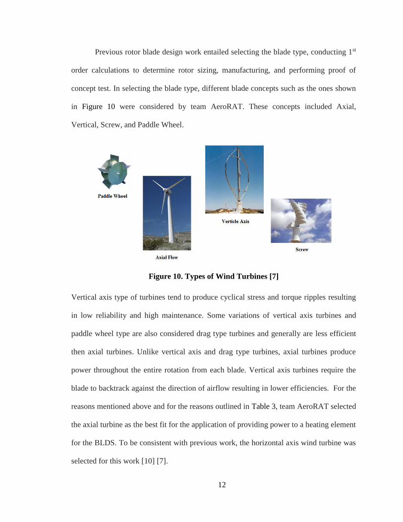
power, and efficiency at varying speeds. Motor specifications for the Maxon brushless

DC motor [14] are displayed in Figure 18, along with performance parameters, the

manufacturer also provides motor performance at a nominal voltage. To evaluate the

motor model; motor no-load current, speed constant and internal resistance values at a

nominal voltage of 24 V, as specified was applied to the model.

Figure 18. Maxon Motor Manufacturer Performance Parameters for BLDC

Motor #386677 [14] [18]

Predicted brake torque and power curves shown in Figure 19 accurately predict no-load

speed to be approximately 29,500 rpm for nominal voltage of 24 V, as specified in motor

performance data in Figure 18.

29

Figure 19. Motor Model Predicted Torque and Brake Power

The predicted motor efficiency curve shown in Figure 20 is also able to accurately predict

maximum efficiency to be approximately 90% (89.44 %) for the published nominal

voltage of 24 V.

Figure 20. Motor Model Predicted Efficiency

30

An efficiency contour chart was also created for different input power values at varying

speeds as seen below in Figure 21. This is useful as a quick look-up chart to estimate

efficiency at a specific power input and speed.

Figure 21. Motor Model Efficiency Contour Chart

2.3 Generator Electrical Model

The electrical diagram of the generator model is illustrated in Figure 22. Note that

the BLDC generators that are being considered, all generate 3 phase power; the schematic

shown in Figure 22 only represents phase-to-phase or two of the three phases. Starting

from the shaft power as the input on the left side of the diagram, the gross or “ideal”

power delivered at the shaft experiences several losses throughout the generator. The

power losses in the generator consist of the following: windage and friction losses which

are accounted for in the no-load current (IO) parameter, motor winding resistance, also

0.70.7

0.7

0.7

0.80.8

0.8

0.8

0.850.85

0.85

0.85

0.88

0.88

0.88

0.9

0.9

RPM

Input

Pow

er

(Watt

s)

Motor Efficiency Contour

0 0.5 1 1.5 2 2.5 3 3.5 4 4.5 5

x 104

0

50

100

150

200

250

300

350

400

450

500

31

known as the internal resistance, (Ri), and inductance reactance losses which are

approximated by multiplying inductance (L) by 2π times the frequency (f) of the

generator. Additionally we have a load (RL), at the terminal that also is accounted for in

the model. At this point power rectification is not yet considered. Power rectification is

not necessary for heating the BLDS. However rectifying would be required if power

generated were to provide power to augment charge, or replace batteries. Power

rectification and how it is applied to the model will be further discussed in Section 2.4.

Figure 22. Generator Model Electrical schematic [8]

The following Equations 19–26 are the generator model equations derived from the

generator circuit diagram shown in Figure 22. This model is used in predicting generator

brake and terminal power as a function of electrical load and speed. Beginning the

generator performance analysis at the armature, with the model input of speed, armature

voltage is calculated in Equation 19.

𝑉𝑎 =𝑅𝑃𝑀

𝐾𝑣 (19)

32

𝐼𝑎 =

𝑃𝑏𝑟𝑎𝑘𝑒𝑉𝑎

(20)

We then calculate the circuit current with the following equation. Here the armature

voltage is divided by the total resistance. Note that the total resistance includes resistance

at the load, generator internal resistance and inductance reactance.

I =𝑉𝑎

𝑅𝐿 + 𝑅𝑖 + 𝑋𝑖𝑛𝑑 (21)

Terminal power can then be calculated using Equation 22

𝑃 = 𝑉𝑡𝐼 (22)

In order to estimate brake torque and power, armature current is solved for using

Equation 23. Note that the armature current is the ideal current without accounting for the

friction and windage losses that are represented by the no-load current; Equation 23

applies these losses in order to solve for the circuit current.

𝐼 = 𝐼𝑎 − 𝐼𝑜 (23)

Rearranging Equation 24, armature current is solved.

𝐼𝑎 = I + 𝐼𝑜 (24)

With armature current known brake power is solved with Equation 20 and torque can be

solved for with Equation 25.

𝑄𝐺 =

𝑃𝑏𝑟𝑎𝑘𝑒ω

(25)

33

Terminal electrical power over input brake power gives the generator efficiency.

𝜂𝑚 =𝑃

𝑃𝑏𝑟𝑎𝑘𝑒 (26)

Now the generator model equations can be used to develop torque, power, and

efficiency curves as shown in Figure 23 and Figure 24.Note that this model is a function

of electrical load and speed – a different performance curve is generated for different

loads at the terminal. For the plots shown in Figure 23 and Figure 24, the model was run

at an electrical load of 5 Ohms for speeds up to 45,000 rpm. The same performance

parameters for the motor used in the motor model are applied– these manufacturer

specifications are displayed in Figure 18.

Figure 23. Generator Model Predicted Torque and Shaft Power at 5 Ohms

0 0.5 1 1.5 2 2.5 3 3.5 4 4.5

x 104

0

0.01

0.02

0.03

0.04

0.05

0.06Generator Brake Torque and Power @ RL=5 Ohms

RPM

Qg (

N-m

)

0 0.5 1 1.5 2 2.5 3 3.5 4 4.5

x 104

0

50

100

150

200

250

300

Pbra

ke (

Watt

)

34

Figure 24.Generator Model Predicted Efficiency at 5 Ohms

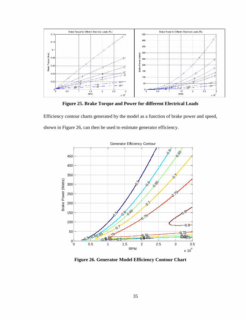
Now for the case where brake torque and power are known and electrical load is

unknown, the model is run for different electrical loads and plotted as shown in Figure

25. Using the charts of Figure 25, electrical load can be determined for a known brake

torque and speed. Looking at the charts of Figure 25, it might seem counter-intuitive that

low torque is predicted at a higher resistance however, it is important to understand that

high resistance means lower electrical load. For example, as resistance goes up less

current flows through the circuit; as resistance approaches infinity, the circuit is

essentially open. Considering this, higher torques are observed at lower resistance and

lower torque at higher resistance.

0 0.5 1 1.5 2 2.5 3 3.5 4 4.5

x 104

0

0.1

0.2

0.3

0.4

0.5

0.6

0.7

0.8

0.9

RPM

Eff

icie

ncy

Generator Efficiency @ RL=5 Ohms

35

Figure 25. Brake Torque and Power for different Electrical Loads

Efficiency contour charts generated by the model as a function of brake power and speed,

shown in Figure 26, can then be used to estimate generator efficiency.

Figure 26. Generator Model Efficiency Contour Chart

0.5 0.50.5

0.5

0.5

0.60.60.60.6

0.6

0.6

0.6

0.65

0.65

0.65

0.65

0.65 0.65 0.65

0.7

0.7

0.7

0.7 0.70.7

0.75

0.75

0.75 0.75

0.75

0.8

0.8

RPM

Bra

ke P

ow

er

(Watt

s)

Generator Efficiency Contour

0 0.5 1 1.5 2 2.5 3 3.5

x 104

0

50

100

150

200

250

300

350

400

450

36

2.4 Power Rectification

For our application of powering a heating element for the BLDS it may be desired

to convert AC current to DC current. This section will now focus on power rectification

and how it is applied in the generator model. Converting AC to DC is primarily done

through the use of diodes which are commonly integrated into rectifier circuits. A diode

is an electrical device that allows current flow through one direction and blocks current in

the opposite direction. The diode is analogous to a mechanical check valve. Typically

diodes are composed of semiconductors with a nonlinear current – voltage relationship,

as shown in Figure 27.

Figure 27. Diode Current - Voltage relationship [19]

As seen in Figure 27 above, semiconductor diodes conduct only when a threshold voltage

or forward voltage has been achieved in the diodes forward direction, also known as

“forward bias”. At voltages lower than the threshold voltage, the diode circuit is

considered open. Whenever we have negative voltage the diode is considered “negative

bias” and acts to block current in the opposite direction with exception of a small leakage

current on the order of milliamps. A negative biased diode will block current until a

37

breakdown voltage has been achieved, at which point current will dramatically increase

in the negative direction.

Diodes are combined to form several types of rectifiers such as half-wave, full-

wave, single-phase and multi-phase. The half-wave rectifier only lets half of the AC

wave through while blocking the other half. Through the integration of 4 diodes the full-

wave rectifier is able to allow the full AC wave through by essentially flipping the

negative half AC wave to positive on the DC side.

Figure 28. Half Wave

Rectification [20]

Figure 29. Full Wave

Rectification [20]

Since the brushless generator produces 3-phase power, a 3-phase full wave rectifier is

used to rectify its output. A 3-phase rectifier is effectively 3 single full wave rectifiers put

together. Referencing Figure 30, it can be seen that the 3-phase rectifier is composed of 6

diodes with each diode having a forward voltage drop of approximately 1.2 volts

(dependent on current).

38

Figure 30. Voltage rectification using 3-phase bridge rectifier [21]

Figure 31 below displays the current-voltage relationship for the rectifiers used in model

evaluation testing (IXYS FUO 22 Three Phase Rectifier Bridge [21]). Using this chart the

forward voltage for each diode may be estimated based on estimated current values. The

diode’s forward voltage can then be applied in the generator model equation, Equation 21

Figure 31. Current - Voltage per Diode in IXYS FUO 22 Three Phase Rectifier

Bridge [21]

39

Because only 1 diode is “on” per phase, the 3-phase rectifier is represented in Figure 8

with only 2 diodes present in the phase-to-phase representation (forward & backward

bias) [9].

Figure 32. Generator Model Electrical Schematic [8] [9]

In going from AC to DC it is important to consider the relationship between peak

voltage (𝑉𝑝𝑒𝑎𝑘), rms voltage (𝑉𝑟𝑚𝑠), and average voltage (𝑉𝑎𝑣𝑒𝑟𝑎𝑔𝑒). Using a (Fluke)

multimeter, measurements are made in rms for AC and average for DC. When applying

generator Equations 19– 26 it is necessary to convert to the appropriate form. Equation

27 describes the relation between 𝑉𝑟𝑚𝑠 and 𝑉𝑝𝑒𝑎𝑘 for a single phase AC signal. Equation

28 describes the relation between 𝑉𝑝𝑒𝑎𝑘 and 𝑉𝑎𝑣𝑒𝑟𝑎𝑔𝑒 and applies to the rectified DC

signal when using a 3-phase rectifier.

𝑉𝑟𝑚𝑠 =𝑉𝑝𝑒𝑎𝑘

√2 (27)

𝑉𝑎𝑣𝑒𝑟𝑎𝑔𝑒 =

3

𝛱𝑉𝑝𝑒𝑎𝑘

(28)

40

Combining both Equations 27 and 28, we get Equation 29 which is the DC

equivalent voltage when going from AC to DC when neglecting the voltage drop across

the rectifier diodes [9].

𝑉𝐷𝐶 = 𝑉𝑎𝑣𝑒𝑟𝑎𝑔𝑒 =3

𝛱√2𝑉𝑟𝑚𝑠 [9] (29)

Now in applying rectifier losses we apply a simplified approach to diode circuit

analysis where a diode is treated as voltage sources once diode threshold voltage is

achieved. Diode internal resistance for this analysis is neglected. In applying the rectifier

losses to the generator model, the circuit current equation is modified to include a voltage

drop for two diodes per phase (Equation 30). For the BLDS heating application it’s

important to remember that the power losses at the rectifier are dissipated as heat and

could be used as a heat source for the BLDS if located within the system.

I =𝑉𝑎 − 2𝑉𝐷𝑂

𝑅𝐿 + 𝑅𝑖 + 𝑋𝑖𝑛𝑑 (30)

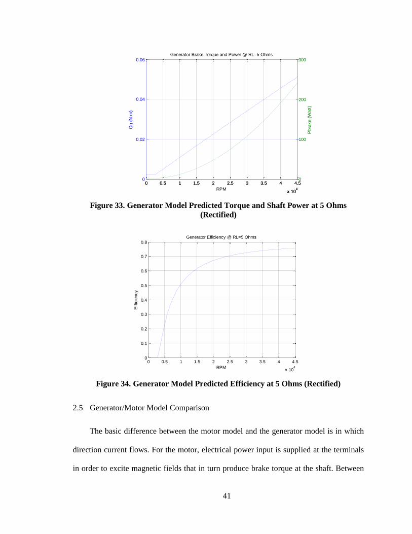
Now with rectifier losses accounted for, brake torque and power curves, shown in Figure

33 and Figure 34, are again generated at an electrical load of 5 Ohms for speeds up to

45,000 rpm. Note that at low speeds where the generated armature voltage is below

rectifier threshold voltage, the circuit is considered open resulting in a constant torque

proportional to the generator no-load current parameter. Comparing model results with

and without rectifier losses applied, it can be seen that the differences are significant. For

example, at 30,000 rpm, without rectifier losses, the model predicts the generator at 80%

efficient; model results with rectifier losses applied predict an efficiency of 72.5%. With

a difference of 7.5% shift in efficiency, it is therefore recommended to include rectifier

losses in the generator model

41

Figure 33. Generator Model Predicted Torque and Shaft Power at 5 Ohms

(Rectified)

Figure 34. Generator Model Predicted Efficiency at 5 Ohms (Rectified)

2.5 Generator/Motor Model Comparison

The basic difference between the motor model and the generator model is in which

direction current flows. For the motor, electrical power input is supplied at the terminals

in order to excite magnetic fields that in turn produce brake torque at the shaft. Between

0 0.5 1 1.5 2 2.5 3 3.5 4 4.5

x 104

0

0.02

0.04

0.06Generator Brake Torque and Power @ RL=5 Ohms

RPM

Qg (

N-m

)

0 0.5 1 1.5 2 2.5 3 3.5 4 4.5

x 104

0

100

200

300

Pbra

ke (

Watt

)

0 0.5 1 1.5 2 2.5 3 3.5 4 4.5

x 104

0

0.1

0.2

0.3

0.4

0.5

0.6

0.7

0.8

RPM

Eff

icie

ncy

Generator Efficiency @ RL=5 Ohms

42

the input power at the terminals and mechanical torque at the shaft, losses due to internal

resistance and frictional torque are applied, resulting in a net mechanical torque.

Alternatively for the generator, a gross input shaft power is supplied at the shaft to

generate an electrical output at the generator terminals. Here due to friction and windage,

mechanical power losses are already incurred before a net power is generated. The

generated power then incurs further losses due to internal resistance and reactance.

Because the power generated is AC, additional resistance due to the change in current

with phase angle known as reactance is experienced. Additionally, rectifier losses will be

applied when converting AC to DC. The table below depicts the major differences in how

terminal power is calculated between both models.

Table 4. Motor/Generator Equation Comparison

Motor Model Generator Model

Terminal Current 𝐼 = 𝐼𝑎 + 𝐼𝑜 𝐼 = 𝐼𝑎 − 𝐼𝑜

Terminal Voltage 𝑉 = 𝑉𝑎 + 𝐼𝑅𝑖 𝑉 = 𝑉𝑎 − 𝐼𝑅𝑖 − 𝐼𝑋𝑖𝑛𝑑 − 𝑉𝑟𝑒𝑐𝑡𝑖𝑓𝑖𝑒𝑟

Armature Current 𝐼𝑎 =𝑃𝑏𝑟𝑎𝑘𝑒𝑉𝑎

Armature Voltage 𝑉𝑎 =𝑅𝑃𝑀

𝐾𝑣

Shaft Torque 𝑄𝐺 =𝑃𝑏𝑟𝑎𝑘𝑒ω

Shaft Power 𝐼𝑎 =𝑃𝑏𝑟𝑎𝑘𝑒𝑉𝑎

Efficiency ηm =PshaftP

ηm =P

Pshaft

43

2.6 Generator Model Evaluation (Validation) Testing

Prior to conducting generator model validation testing, it is necessary to first verify

generator manufacturer specifications such as Kv, Ri and Io. In verifying the speed

constant (Kv), the test setup of Figure 35 was implemented. Here the Line-to-Line

voltage and RPM are measured as the generator is rotated at different speeds by another

motor. The voltage is measured at any two lead wires from the generator with no load

electrical load at the terminals.

Figure 35. Generator Kv Test Schematic

Figure 36 shows an annotated photograph of the test schematic given in Figure 35.

44

Figure 36. Generator Kv Test Setup

Because the Fluke multimeter reads voltage in true rms, Equations 31 & 32 are used

to determine peak voltage. Peak voltage is desired in verifying Kv because the Line-to-

Line voltage represents the Armature voltage or back emf (shown in Figure 32) and it is

from this peak voltage that losses are applied to, before converting to DC. RPM is

measured by reading the frequency of one of the generator lead wires and converting to

RPM using Equation 26. This method of reading the frequency from one of the

generators lead wires is most accurate above 8,000 RPM. Measurements taken below this

value tend to be noisy and not reliable due to poor signal amplitude at or below this

speed. Kv is then calculated with Equation 32.

𝑅𝑃𝑀 =𝑓 ∗ 2 ∗ 60

# 𝑝𝑜𝑙𝑒𝑠 (31)

𝐾𝑉 =

𝑅𝑃𝑀

𝑉𝑎

(32)

45

Table 2 displays results for the Kv verification test for the generator at various

speeds. The average measured Kv value for this generator was determined to be 1230

RPM/volts with a standard deviation of 1,288 RPM/volts.This value for Kv matched the

manufacturer specified Kv of 1230 RPM/volts.

Table 5. Generator Kv Verification Results

Prime Mover Input Generator

Volts I (Amps) f(Hz) RPM Voltage (RMS) Voltage (peak) Kv (peak) Variance

5.01 2.8 181.9 10914 6.2 8.8 1238.7 74.2

6.02 3.2 225.8 13548 7.8 11 1231.3 1.5

7.01 3 265 15900 9.2 13 1226.1 16.5

8.02 3 306.9 18414 10.6 15 1227.2 8.5

9.06 3.1 349.1 20946 12.1 17 1229.1 1.0

10.03 3.1 389.9 23394 13.5 19 1229 1.3

11.01 3.2 430.9 25854 14.9 21 1229.4 0.5

𝑲𝑽(𝑨𝒗𝒆𝒓𝒂𝒈𝒆) = 𝟏𝟐𝟑𝟎 (𝒓𝒑𝒎/𝑽) 𝐒𝐭𝐚𝐧𝐝𝐚𝐫𝐝 𝐃𝐞𝐯.= 1,288 (𝑟𝑝𝑚/𝑉)

Internal resistance is indirectly verified according to the schematic of Figure 37,

where a power source is connected directly to generator lead wires. To avoid burning up

the generator a power resistor is connected in series. Generator internal resistance is

measured indirectly by measuring current and voltage drop across the generator lead

wires when a DC voltage source is supplied to the circuit. The voltage input for this test

was 8 volts and was not varied since input voltage should not affect results. The

measured current and voltage values at the generator are then used to calculate the

internal resistance as displayed in Table 6. As shown in Table 6, measurements were

taken for each wire pair and averaged to get an internal resistance value of 0.271 ohms.

46

Figure 37. Electrical Schematic of Generator Internal Resistance Measurement

𝑹𝒊 =

𝑽

𝑰

(33)

Table 6. Internal Resistance Measurement Results

Lead Wire pairs

Volts I (Amps) Ri (Ohms)

orange/brown 0.196 0.725 0.270

orange/red 0.127 0.4671 0.272

red/brown 0.127 0.4668 0.272

𝑅𝑖(𝐴𝑣𝑒𝑟𝑎𝑔𝑒) = 0.271 𝑂ℎ𝑚𝑠

A comparison of manufacturer published specifications to the measured values is

displayed in Table 7. While it would be ideal to also verify the no-load current Io, we did

not have the speed controller for this specific generator in order to run it as a motor and

measure no load current. With a close match between published and measured Kv and Ri

47

values it was expected that the no-load parameter also match closely to the published

value; therefore it was decided to not verify no-load current and treat it as a constant

unless subsequent generator evaluation tests suggested that it was necessary to do so.

Table 7. Generator Parameter Verification

Manufacture specifications

Measured

Kv 1230 1230

Ri 0.269 0.27

Following the verification of the speed constant and internal resistance, the

generator model was evaluated using the test setup depicted in Figure 38-Figure 39.

Similar to the test setup in measuring Kv, the prime mover rotates the generator at

varying speeds through the shaft coupler. In evaluating the generator model, the AC

voltage out of the three generator lead wires is put through the three-phase rectifier and a

resistive electrical load. At the load, voltage and current are measured. The test were

conducted at a fixed load resistance for a range of RPM at increments of about 1,000

RPM, then repeated for another fixed load resistor. Resistance for the load was measured

using a Fluke multi-meter.

48

Figure 38. Generator Test Schematic

Figure 39. Generator Test Setup

Figure 40 and Table 8 show results of the generator evaluation test at an electrical

load of 3.02 Ohms and compares those results to the calculated values using the generator

model. It is observed that predicted terminal power values are within a few percent of

measured values with an uncertainty below 2%.

49

Figure 40. Generator Model Test Results at 3.02 Ohms

Table 8. Generator Model Test Results at 3.02 Ohms

f(Hz) RPM

Calculated Parameters Measured Parameters

% Error I (Amps) Vr (Volts) Power(Watts) I(Amps) Vr (Volts) Power(Watts)

163.5 9810 1.72 5.18 8.89 1.75 5.25 9.19 -3.24

178.9 10734 1.93 5.83 11.24 1.977 5.9 11.66 -3.62

196.3 11778 2.17 6.55 14.23 2.21 6.64 14.67 -3.06

215.1 12906 2.43 7.34 17.83 2.467 7.38 18.21 -2.05

234.3 14058 2.69 8.14 21.93 2.72 8.15 22.17 -1.08

251.6 15096 2.93 8.86 25.97 2.95 8.85 26.11 -0.52

268.8 16128 3.17 9.57 30.32 3.19 9.54 30.43 -0.38

288.2 17292 3.43 10.37 35.61 3.49 10.31 35.98 -1.03

306.2 18372 3.68 11.11 40.89 3.69 11.05 40.77 0.28

323.3 19398 3.91 11.82 46.23 3.91 11.71 45.79 0.96

344.4 20664 4.14 12.51 51.82 4.19 12.54 52.54 -1.38

361.8 21708 4.38 13.22 57.89 4.41 13.23 58.34 -0.78

380.6 22836 4.63 13.99 64.81 4.657 13.95 64.97 -0.25

401.6 24096 4.92 14.85 72.97 4.92 14.76 72.62 0.49

420.9 25254 5.18 15.63 80.88 5.17 15.56 80.45 0.55

While generator model evaluation test results provide confidence in the generator

model’s ability to accurately predict generator electrical performance at a given rpm, it

0

10

20

30

40

50

60

70

80

90

8000 10000 12000 14000 16000 18000 20000 22000 24000 26000 28000

Po

wer

(w

atts

)

RPM

Terminal Power with Electrical Load RL=3.02 ohms

Power_Calculated

Power_Measured

50

does not provide an evaluation of the model prediction of generator shaft torque. The

only direct way to verify torque would be to directly measure it using an in-line shaft

torque transducer or perhaps a torque cradle. An alternative approach that will not

measure torque directly but will give some indication of whether the generator model is

producing good estimates for brake torque is to calculate brake torque for a given

motored generator test, separate from the generator model, using the dc motor model for

the prime mover, then compare torque values to the torque predicted by the generator

model. To do this, it is first necessary to implement the DC motor equations (Chapter 2.2)

to predict brake torque for the prime mover. Prior to applying the motor model equations

it is first necessary to verify motor manufacturer specifications for Kv, Ri and Io.

Because the motor that is being used as the prime mover is 2+ years old and has already

experienced significant wear, the motor parameters are expected to deviate from the

manufacturer specifications. The motor parameters were measured in the same manner as

those for the generator, except that it was possible to measure Io. Table 9 displays the

manufacturer specified parameters and the measured values. Here we see that the Kv

parameter significantly deviates from what the manufacturer specified with a 38% error.

A possible explanation of for this significant deviation in Kv is loss of performance of the

permanent magnets due to overheating or over magnetizing. Note that the manufacturer

did not provide a value for internal resistance for this motor. Also, after measuring the

no-load current, it was determined that the actual no-load current value significantly

varied linearly with speed and is not a constant 1.9 Amps as the manufacturer specified.

Because measured No-Load current is not constant it was excluded from Table 9 and is

instead shown in Figure 41.

51

Table 9. Motor Parameter Verification [Ammo BLDC (part# 35-56-1800kv)]

Manufacture

specifications Measured

Kv [RPM/volts] 1800 2491.33

Ri [ohms] - 0.20012

Io [amps] 1.9 -

The no-load current for the DC motor is plotted below in Figure 41. Because the no-

load current varies linearly with speed, a trend line was set and used in calculating motor

torque output at various speeds. In the motor model the linear fit was used to establish the

input no-load current for the corresponding velocity. Because for this motor the no-load

current varied significantly with speed, here the no-load was not applied in the motor

model as a constant and varied with speed as depicted in Figure 41.

Figure 41. DC Motor No-Load Current

y = 3E-05x + 2.0626

0

0.5

1

1.5

2

2.5

3

3.5

0 5000 10000 15000 20000 25000 30000 35000

No

-Lo

ad C

urr

ent

(Am

ps)

RPM

52

Now for a motored generator test where the Ammo BLDC (part# 35-56-1800kv) motored

the Maxon generator with a 2.3 ohm electrical load at the terminal, DC motor brake

torque and power values were predicted using motor model Equations 12 through 18.

Inputs to the model were speed and voltage – output results can be seen below in Table

10.

Table 10. DC Motor Shaft Torque Calculation

P (watts) V

(volts) I (amps) f (Hz) RPM

Io (amps)

Ia (amps)

Va (volts)

Pbrake (watts)

Eta (%) Torque (N-m)

28.80 4.5 6.4 156.9 9414 2.31 4.09 4.37 17.87 62.03 0.018

36.00 5 7.2 173.6 10416 2.34 4.86 4.86 23.60 65.55 0.022

42.90 5.5 7.8 190.4 11424 2.37 5.43 5.34 29.03 67.68 0.024

49.80 6 8.3 208.6 12516 2.40 5.90 5.83 34.44 69.16 0.026

57.85 6.5 8.9 226.5 13590 2.43 6.48 6.32 40.94 70.76 0.029

66.50 7 9.5 243.75 14625 2.45 7.05 6.81 47.99 72.17 0.031

75.75 7.5 10.1 261.8 15708 2.48 7.62 7.30 55.60 73.4 0.034

85.60 8 10.7 280.4 16824 2.51 8.19 7.79 63.76 74.48 0.036

96.05 8.5 11.3 300.3 18018 2.54 8.76 8.27 72.46 75.43 0.038

108.00 9 12 317.2 19032 2.57 9.43 8.76 82.61 76.49 0.041

119.23 9.5 12.55 337 20220 2.60 9.95 9.25 92.01 77.17 0.044

136.00 10 13.6 354.7 21282 2.63 10.97 9.73 106.72 78.47 0.048

142.80 10.5 13.6 374.7 22482 2.66 10.94 10.23 111.87 78.34 0.048

Brake torque values are then calculated independently from the motor model using the

generator model with with terminal load of 2.33 ohms. Brake torque values calculated

through the generator model are displayed in Table 11. Torque predictions from both the

motor and generator models are then compared in Figure 43 and with a percent difference

shown in Table 12.

53

Figure 42. Torque Verification diagram

Table 11. Generator Shaft Torque Calculation

54

Table 12. Motor/Generator Shaft Torque

f(Hz) RPM Motor Torque (N-m) Generator Torque (N-m) % Diff

156.9 9414 0.018 0.019 3.15

173.6 10416 0.022 0.021 2.61

190.4 11424 0.024 0.023 3.39

208.6 12516 0.026 0.026 0.94

226.5 13590 0.029 0.029 0.73

243.75 14625 0.031 0.031 1.15

261.8 15708 0.034 0.034 0.87

280.4 16824 0.036 0.036 0.23

300.3 18018 0.038 0.039 1.23

317.2 19032 0.041 0.041 0.55

337 20220 0.043 0.043 0.17

354.7 21282 0.048 0.046 4.39

374.7 22482 0.048 0.049 2.20

Figure 43. Motor and Generator Model Predicted Shaft Torque

0

0.01

0.02

0.03

0.04

0.05

0.06

0 5000 10000 15000 20000 25000

Torq

ue

[N-M

]

RPM

Motor and Generator Model Predicted Shaft TorqueMotor TorqueGenerator Torque

55

In addition to computing shaft torque independently through the prime mover motor

model and the generator model, both models can be coupled in series beginning with the

source power to the DC motor as an input and terminal power as an output. Input power

and current were measured at the source using two Fluke multi-meters. The power losses

at the speed controller were neglected and assumed to be minimal since the controller

was set to maximum and instead the power source was used as the actual control by

varying voltage for all trials . Generator output power is then calculated through the

coupled motor and generator models and compared to actual measured terminal power

values. Terminal voltage and current were also measured using Fluke multi-meters at the

terminal load.

Figure 44. Motor to Generator Model Validation Test Diagram

Table 13. Motor to Generator Terminal Power Calculation

RPM V I Pshaft Torque (N-m) P (watts)

9414 4.5 6.4 17.87 0.018 7.654 2.334 2.071 1.978 4.89 4.67 9.24

10416 5 7.2 23.60 0.022 8.468 2.787 2.524 2.41 5.58 5.33 12.85

11424 5.5 7.8 29.03 0.024 9.288 3.126 2.863 2.734 6.31 6.03 16.47

12516 6 8.3 34.44 0.026 10.176 3.385 3.122 2.981 7.13 6.81 20.29

13590 6.5 8.9 40.93 0.029 11.049 3.705 3.442 3.287 7.91 7.56 24.84

14625 7 9.5 47.99 0.031 11.89 4.036 3.773 3.603 8.66 8.27 29.81

15708 7.5 10.1 55.60 0.034 12.771 4.354 4.091 3.906 9.46 9.03 35.28

16824 8 10.7 63.76 0.036 13.678 4.661 4.398 4.2 10.28 9.82 41.23

18018 8.5 11.3 72.45 0.038 14.649 4.946 4.683 4.472 11.17 10.67 47.71

19032 9 12 82.61 0.041 15.473 5.339 5.076 4.847 11.89 11.35 55.03

20220 9.5 12.55 92.01 0.043 16.439 5.597 5.334 5.094 12.78 12.21 62.18

21282 10 13.6 106.71 0.048 17.302 6.168 5.905 5.639 13.49 12.88 72.64

22482 10.5 13.6 111.87 0.048 18.278 6.121 5.858 5.594 14.48 13.83 77.34

MOTOR GENERATOR 𝐚 ( 𝐞𝐚 ) ( 𝐞𝐚 ) 𝐚 ( 𝐞𝐚 ) (𝐃 ) 𝐫 ( 𝐞𝐚 ) (𝐃 )

56

Table 14 compares calculated terminal power from the motor to generator model to

actual measured terminal power. It can be seen that the percent error is typically a few

percent and everywhere within 10%. Based on the condition of the motor and how its

performance parameters varied significantly with RPM, it can be assumed that the

majority of the error is at the motor. Although a percent error less than a few percent

establishes confidence in both motor and generator models, direct torque measurements

would still be desirable to fully evaluate the model.

Table 14. Motor to Generator Model Calculated Terminal Power Compared to

Actual

CALCULATED MEASURED % Error f (Hz) RPM I (DC) V (DC) P (DC) I (DC) V (DC) P (DC)

156.9 9414 1.98 4.61 9.11 2.08 4.8 9.98 -8.76

173.6 10416 2.41 5.24 12.64 2.4 5.49 13.18 -4.10

190.4 11424 2.73 5.92 16.17 2.69 6.15 16.54 -2.24

208.6 12516 2.98 6.67 19.90 3 6.87 20.61 -3.46

226.5 13590 3.29 7.40 24.32 3.3 7.57 24.98 -2.65

243.75 14625 3.60 8.09 29.14 3.6 8.25 29.70 -1.88

261.8 15708 3.91 8.81 34.43 3.9 8.93 34.83 -1.13

280.4 16824 4.20 9.57 40.19 4.21 9.65 40.63 -1.09

300.3 18018 4.47 10.38 46.44 4.54 10.4 47.22 -1.64

317.2 19032 4.85 11.03 53.45 4.82 11.05 53.26 0.36

337 20220 5.09 11.84 60.33 5.15 11.81 60.82 -0.80

354.7 21282 5.64 12.46 70.25 5.43 12.44 67.55 4.00

374.7 22482 5.59 13.38 74.85 5.76 13.19 75.97 -1.47

57

3. ROTOR MODEL

A rotor model based on simple blade element theory has been developed with the

intention of establishing a baseline rotor design tool that can take a given rotor geometry

and rotation rate; and predict torque created on the rotor by aerodynamic forces at a given

relative airspeed. This tool will allow variation of rotor design parameters such as number

of blades, hub and tip diameter, blade angle, blade twist, and taper to effectively predict

rotor performance; enabling rotor optimization and rotor/generator performance

matching. Classical momentum theory and blade element analysis are employed in

predicting rotor performance for a given size and geometry; the induced flow caused by

the rotor wake and aero-elastic rotor blade deformation are neglected in this analysis.

Also note that the analysis can be applied to both propellers or turbines and that

prediction values will be positive for a propeller and negative for a turbine. A second

rotor analysis tool, Drela & Youngren open source model, X-Rotor [22] is also being

used. X-Rotor includes the influence of the wake’s induced flow, and is therefore

assumed to provide more accurate results. However, X-Rotor also does not include aero-

elastic blade deformation under load. Both analysis tools employ user-input data for

blade section lift and drag. For the present case, that data is only crudely approximated.

The following subsections detail on the actuator disk analysis used in determining max

theoretical performance; the blade element model used to predict rotor performance; and

the X-Rotor performance predictions and how they compare to results obtained from the

blade model [22].

58

3.1 Actuator Disk Theory

A simple one-dimensional (no swirl) steady, inviscid model based on Newton’s 2nd

law is used to establish maximum theoretical performance of an ideal rotor at various

operating conditions. This model considers a control volume with streamtube boundaries

and two cross-sections as the inlet and outlet; represented as control volume 1-4 in Figure

45. The ideal “bare” (unducted) rotor is represented as uniformly loaded, permeable,

infinitely thin actuator disk. Control volumes before and after the actuator disk are also

considered in this analysis; shown in Figure 45 as control volumes 1-2 and 3-4 [13].

Figure 45. Turbine Actuator Disk

59

In applying the actuator disk analysis, it is assumed that pressure far upstream and

downstream are equal and equivalent to the surrounding ambient pressure.

𝑝1 = 𝑝4 (34)

Velocity across the actuation area is assumed equal, with a discontinuity in pressure as

shown in Figure 45.

𝑈2 = 𝑈3 (35)

First, Bernoulli’s equation is applied to control volumes 1-2 and 3-4.

𝑝1 +1

2𝜌𝑈1

2 = 𝑝2 +1

2𝜌𝑈2

2 (36)

𝑝3 +1

2𝜌𝑈3

2 = 𝑝4 +1

2𝜌𝑈4

2 (37)

The change in pressure fore and aft of the actuator disk is solved for by combining

equations 36 and 37 as shown below

𝑝3 − 𝑝2 =1

2𝜌(𝑈4

2 − 𝑈12) (38)

Applying Newton’s 2nd law to the actuator disk at 2-3, the net thrust is calculated. The

thrust force is an axial force on the actuator disk as a result of momentum change and

will result as negative for a wind turbine.

𝑇 = 𝑃3𝐴3 − 𝑃2𝐴2

𝑇 = (𝑝3 − 𝑝2)𝐴𝑑𝑖𝑠𝑘

(39)

Alternatively, thrust is determined by applying conservation of momentum to calculate

the change in momentum between control areas 1-4

60

𝑇 = �̇�𝑈4 − �̇�𝑈1

𝑇 = �̇�(𝑈4 − 𝑈1)

(40)

Substituting Equation 38 and equating Equations 39 and 40, the velocity at the actuator

disk can be solved for:

(𝑝3 − 𝑝2)𝐴𝑑𝑖𝑠𝑘 = �̇�𝑈4 − �̇�𝑈1

1

2𝜌(𝑈4

2 − 𝑈12)𝐴𝑑𝑖𝑠𝑘 = �̇�(𝑈4 − 𝑈1)

(41)

Simplifying we get equation (42), which shows that the velocity at the disk is the average

airspeed between upstream and downstream.

𝑈2 =(𝑈4 + 𝑈1)

2 (42)

Here we introduce the axial induction factor (a), which represents the fractional change in

airspeed between the freestream and the actuator disk face; for a turbine, (a) is negative.

𝑎 = ((𝑈2 − 𝑈1)

𝑈1) (43)

Equation 43 can then be rearranged to solve for velocity at the disk face in terms of

induction factor

𝑈2 = 𝑈1(1 + 𝑎) (44)

Substituting equation 44 into 42 will solve for downstream velocity, equation (45). From

this equation it can be seen that downstream velocity decreases to zero as the inflow

factor approaches -0.5.

61

𝑈4 = 𝑈1(1 + 2𝑎) (45)

With downstream velocity solved for, an energy balance for the 1-4 control volume can

be applied in order to solve for power.

𝑃𝑒𝑥𝑡𝑟𝑎𝑐𝑡𝑒𝑑 =1

2 �̇�𝑈4

2 −1

2�̇�𝑈1

2 (46)

After substituting for mass flow rate, extracted power can be calculated in equation 47

𝑃𝑒𝑥𝑡𝑟𝑎𝑐𝑡𝑒𝑑 = 𝜌𝐴𝑑𝑖𝑠𝑘(𝑈1 + 𝑈4)

2∗(𝑈2

4− 𝑈1

2)

2 (47)

Coefficient of power and thrust is then calculated using the customary definition for a

wind turbine: by dividing power extracted by power available in the freestream for a

given swept area.

𝐶𝑃 =𝑃𝑒𝑥𝑡𝑟𝑎𝑐𝑡𝑒𝑑𝑃𝑎𝑣𝑎𝑖𝑙𝑎𝑏𝑙𝑒

=𝑃𝑒𝑥𝑡𝑟𝑎𝑐𝑡𝑒𝑑

(𝜌𝑈13𝐴𝑑𝑖𝑠𝑘)

12

(48)

𝐶𝑇 =𝑇ℎ𝑟𝑢𝑠𝑡

𝐷𝑦𝑛𝑎𝑚𝑖𝑐 𝐹𝑜𝑟𝑐𝑒=

12𝜌(𝑈4

2 − 𝑈12)𝐴𝑑𝑖𝑠𝑘

𝜌(𝑈42 − 𝑈1

2)𝐴𝑑𝑖𝑠𝑘12

(49)

We are now able to calculate the maximum theoretical coefficient of power by taking the

derivative of Equation 48, setting it equal to zero and solving for (a). At an induction

factor of 𝑎 = −1/3, 𝐶𝑃,𝑚𝑎𝑥 = .59. This value is also known as Betz Limit [13] ; this

value is the maximum theoretical power that can be extracted from the freestream air for

a given swept area. Note that for a turbine the induction factor is negative due to the

velocity decreasing from the streamtube inlet to the face of the actuator disk, whereas for

a propeller this factor is positive. Figure 46, displays 𝐶𝑃 and 𝐶𝑡 as a function of induction

62

factor. In Figure 47 𝐶𝑃 is plotted for a 3.25 in. diameter disk at freestream airspeed of

160 ft/s at standard sea level conditions.

Figure 46. Power and Thrust Coefficients

Figure 47. Power Curve for a 3.25 in. Diameter Rotor

Reality suggests that the Betz Limit will not be attained due to non-ideal conditions such

as viscous drag, rotating wake (“swirl”), having a finite number of blades, and turbine tip

losses that deduct from 𝐶𝑃,𝑚𝑎𝑥 . However, this analysis does provide an upper bound on

63

predicted power extracted and will give a good idea of the turbine sizing requirements for

a desired extracted power. In Figure 48, power extracted has been predicted using

actuator disk analysis for the baseline rotor which is 3.25 inches in diameter. As shown

below, the analysis was conducted at different altitudes, at four different airspeeds. At the

vertical dotted line in each plot below, respective Betz limits are identified [11] [13].

𝑈1 = 50 𝑓𝑡/𝑠 𝑈1 = 100 𝑓𝑡/𝑠

𝑈1 = 150 𝑓𝑡/𝑠 𝑈1 = 200 𝑓𝑡/𝑠

Figure 48. Actuator Disk Power Extracted for Different Axial Velocities at Varying

Axial Induction Factors. (Dotted Line Represents Betz Limit)

-0.5 -0.45 -0.4 -0.35 -0.3 -0.25 -0.2 -0.15 -0.1 -0.05 0

-7

-6

-5

-4

-3

-2

-1

0

Axial Induction Factor (a)

Pow

er

Extr

acte

d (

Watt

s)

sea level

20000 [ft]

30000 [ft]

40000 [ft]

50000 [ft]

-0.5 -0.45 -0.4 -0.35 -0.3 -0.25 -0.2 -0.15 -0.1 -0.05 0

-60

-50

-40

-30

-20

-10

0


Pow

er

Extr

acte

d (

Watt

s)

sea level

20000 [ft]

30000 [ft]

40000 [ft]

50000 [ft]

-0.5 -0.45 -0.4 -0.35 -0.3 -0.25 -0.2 -0.15 -0.1 -0.05 0

-200

-180

-160

-140

-120

-100

-80

-60

-40

-20

0


Pow

er

Extr

acte

d (

Watt

s)

sea level

20000 [ft]

30000 [ft]

40000 [ft]

50000 [ft]

-0.5 -0.45 -0.4 -0.35 -0.3 -0.25 -0.2 -0.15 -0.1 -0.05 0

-450

-400

-350

-300

-250

-200

-150

-100

-50

0


Pow

er

Extr

acte

d (

Watt

s)

sea level

20000 [ft]

30000 [ft]

40000 [ft]

50000 [ft]

64

3.2 Blade Element Theory

In establishing a rotor model, a basic blade element analysis was conducted in order

to predict rotor performance for a given rotor geometry and rotation rate at a specified

airspeed. Unlike actuator disk theory, blade element theory considers a finite number of

blades and involves the partitioning of rotor blades into independent sections along the

length of the blade as shown in Figure 49.

Figure 49. Schematic of Rotor Blade Partitioned into Blade Elements [13]

At each section, thrust and torque are calculated through a force balance that is

conducted using 2-D airfoil lift and drag data. Each section is analyzed independently of

the other assuming no aerodynamic interaction between sections. Sectional thrust and

torque values can then be summed up in order to predict the performance of the entire

rotor. This analysis is limited to 2-D, incompressible flow and does not take into account

induced flow effects. Induced flow effects refers to the spanwise flow associated with an

airfoil of finite aspect ratio. The effects are commonly known as vortices which lie along

the span of an airfoil and extend downstream. Effects of these vortices include a

downward component of velocity that is known as “downwash”. Downwash results in the

change in direction of the relative air stream. The rotation of airflow due to downwash

65

effectively decreases the angle of attack. The blade model presented does not account for

this phenomenon However, it should be sufficient to get a rough approximation of rotor

performance [13] [11].

Figure 50. Blade Velocity and Force Breakdown [12]

In conducting blade element analysis the inner most element is analyzed first. It is

first necessary to determine relative velocity 𝑉1over the blade; for this, axial and

tangential velocity components must be determined. Recalling from blade actuator

theory, velocity undergoes a fractional decrease in velocity from the streamtube inlet to

the face of the disk. This decrease in velocity is characterized by an axial induction factor

which is negative for turbines. Below in equation (50), the axial velocity component at

the face of the disk is the freestream velocity plus the freestream velocity multiplied by

the induction factor [13] [12].

𝑉𝑜 = 𝑉∞(1 + 𝑎) (50)

The angular velocity component is dependent on the blades’ angular velocity. Here an

angular induction factor 𝑏 is introduced. This factor was not previously considered in

actuator disk theory because the flow was assumed 1-dimensional (no swirl). For a

turbine the angular induction factor b is also negative.

66

𝑉2 = 𝜔𝑟(1 − 𝑏) (51)

Once the axial and angular velocity components have been solved for, the resultant

relative velocity is calculated in equation 52.

𝑉1 = √𝑉𝑜2 + 𝑉2

2 (52)

Angle of attack 𝛼 is the angle between the airfoil chord line and relative velocity. Now

that relative velocity has been determined, 𝛼 can now be calculated through Equation 54,

where 𝜃, is the blade angle and 𝜑 is the relative velocity angle and also the angle between

airfoil lift and thrust.

𝜑 = 𝜃 − 𝛼 (53)

Equation 53 is rearranged to solve for 𝛼:

𝛼 = 𝜃 − tan−1𝑉𝑜𝑉2

(54)

Sectional thrust and torque equations are written below, where sectional lift (𝑙) and drag

(𝑑) forces are portioned to thrust and torque.

∆𝑇 = (𝑙 cos ∅ − 𝑑 sin∅) (55)

∆𝑄 = (𝑑 cos ∅ − 𝑙 sin ∅)𝑟 (56)

Lift and drag are calculated in equations (57) and (58) below, where 𝑐 is the chord length,

and 𝐶𝑙and 𝐶𝑑are the sectional coefficients of lift and drag, respectively.

67

𝑙 = 𝐶𝑙1

2𝜌𝑉1

2𝑐𝑑∆𝑟 (57)

𝑑 = 𝐶𝑑1

2𝜌𝑉1

2𝑐∆𝑟 (58)

Below lift and drag equations (57) and (58) have been substituted into equations (55) and

(56) to solve for thrust and torque.

∆𝑇 =1

2𝜌𝑉1

2𝑐(𝐶𝑙 cos ∅ − 𝐶𝑑 sin ∅)𝐵∆𝑟 (59)

∆𝑄 =1

2𝜌𝑉1

2𝑐(𝐶𝑙 cos ∅ + 𝐶𝑑 sin ∅)𝐵𝑟∆𝑟 (60)

We now apply conservation of momentum to develop thrust and torque equations

considering the streamtube control volume 1-4 as depicted in Figure 45

∆T = 𝜌2𝜌𝜋𝑉𝑜(𝑉4 − 𝑉∞) (61)

𝑉𝑜 =

(𝑉∞ + 𝑉4)

2

⇒ 𝑉4 = 𝑉∞(1 + 2𝑎)

(62)

∆𝑇 = 𝜌4𝜋𝑟𝑉∞2𝑎(1 + 𝑎)∆𝑟 (63)

∆𝑄 = 𝜌4𝜋𝑟3𝑉∞𝑏(1 + 𝑎)𝜔∆𝑟 (64)

Thrust and torque equations developed through conservation of momentum are now

equated with those developed in the force balance (Equations 59 and 60) in order to solve

for axial and angular induction factors 𝑎 and 𝑏. As outlined in Figure 51, the process

between equations 50 and 64 is iterated until induction factors converge within a

specified tolerance.

68

Figure 51. Blade Element Model Iteration Diagram

Once induction factors for each blade element have converged, sectional thrust, torque

and power are summed to represent the total thrust and power generated by the entire

rotor.

𝑇 =∑∆𝑇 (65)

𝑄 =∑∆𝑄 (66)

𝑃 =∑∆𝑄 ∗ 𝜔 (67)

Inputs to the blade model include rotor diameter, blade angle, chord, blade twist;

and 𝐶𝑙 and 𝐶𝑑values as functions of angle-of-attack and Reynolds number for a particular

airfoil. For the baseline rotor design, the goal was to select rotor geometry for a low

69

solidity rotor with a diameter as big as would be acceptable in the Cal Poly 2x2 ft wind

tunnel; and to select one “simple” and one more complex blade geometry as a test of the

design tools. Target rpm and power ranges that were aimed for with the rotor design were

between 15,000 and 30,000 rpm; and up to 150 watts of generated power. These target

operating ranges were based off size and operational limitations of available off-the-shelf

generators.

Geometric parameters for the two candidate evaluation rotors selected; are shown in

Table 15.

Table 15. Rotor Geometric Parameters

Rotor 1 Rotor 2

Number of Blades: 3 3

Hub Diameter: 1 in 1 in

Tip Diameter: 3.25 in 3.25 in

Chord: 13 mm 13 mm

Airfoil (NACA): 2412 2412

Re: 80,000 80,000

Root Blade Angle: 25° 40°

Tip Blade Angle: 25° 15°

Twist Distribution: None Linear

Rotor 1 Rotor 2

Figure 52. Baseline Rotors 1 & 2

70

It was decided to analyze two different rotors: one with twist (Rotor 2), and one

with no twist (Rotor 1). Rotor 2 has a linear twist distribution with 25° of blade twist. The

blade angle for Rotor 1 is approximately equal to the blade angle of Rotor 2 at two-thirds

length from the blade root. This was determined based on the assumption that the

majority of thrust and torque is produced in that region of the blade. It is estimated that

with the straight blade rotor partially operating under stalled conditions, that the twisted-

blade rotor, which maintains angle of attack at or near L/D max, will generate more

power at its design RPM.

The airfoil selected for the candidate rotors was the NACA 2412; shown in Figure

53. This airfoil was also used in previous proof-of-concept work.

Figure 53. Selected Rotor Blade Airfoil (NACA 2412)

For the Naca 2412 airfoil, coefficient of lift and drag values were extracted from the

QBlade v0.6 software [23]. QBlade is an open source turbine calculation software that is

integrated into Drela’s airfoil and analysis tool, XFOIL [24]. Rather than using XFOIL

directly, it was decided to use QBlade since it provides a simpler graphical user interface

(GUI) for generating airfoil lift and drag polars using the XFOIL source code [23] [22].

71

Figure 54. QBlade GUI for Analyzing Airfoil CL and CD [23] [22]

The XFOIL code is able to analyze both viscous and inviscid flow over a 2-D airfoil and

provide lift and drag predictions for angles-of-attack beyond CLmax. Although the lift

and drag predictions are within the range of interest for any aircraft or turbine that

maintains the airfoil within the pre-stall range, slow axial airspeeds will drive turbines to

operate with partially stalled blades. This is especially prevalent in rotors that have a

fixed blade angle with no blade twist. Additionally, blade element models will typically

temporarily iterate through post-stall angles of attack. In order to accommodate the

analysis of partially stalled rotor blades and the application of blade element codes, it is

necessary to extend the angle-of-attack range to ± 180°. QBlade offers an extrapolation

module that can be used to extrapolate XFOIL generated lift and drag polars within the

72

pre-stall region to ± 180°. The program offers two methods of extrapolation; the

Montgomery extrapolation and the Viterna-Corrigan post stall model [23] [22].

Figure 55. Montgomery Extrapolated NACA 2412 Lift and Drag curves at

Re:80,000; Using QBlade Extrapolation Module [23] [22]

For this analysis, the Montgomery extrapolation was selected. For this method, lift and

drag curves within the pre-stall range are needed – these are generated and extracted from

XFOIL. The extrapolation is then conducted with the assumption that flow near or around

0° and 180° behaves linearly and can be treated as potential flow, at other angles-of-

attack flow is assumed to approximately behave like a stalled, thin plate. As seen in

73

Figure 56 transformation function is generated to blend both the potential flow straight

line and the flat plate curve.

Figure 56. Blending Function for Combining Potential and Thin Plate Flow for

Montgomery Extrapolation Method [25]

Because we are more concerned with turbine performance with unstalled blades, it is

sufficient to visually form the blending function using the sliders provided by the QBlade

360° extrapolation module user interface. The methodology in which QBlade develops

this extrapolation is detailed in reference [25].

Along with realizing the need to extrapolate lift and drag polars, it is also important

to identify the need to invert the airfoil orientation as compared to that used for a

propeller or fan. For a turbine, blades will be operating at negative angles of attack. At

negative angles of attack, it is desired to invert the airfoil in order to attain the desired lift

and drag performance . The inverted NACA 2412 airfoil along with the inverted 𝐶𝑙

values are shown in Figure 57 below.

74

Figure 57. Inverted NACA 2412 [23] [22]

Blade element model torque and power predictions for the straight blade (Rotor 1)

and twisted blade (Rotor 2) rotors are shown in Figure 58 and Figure 59, respectively.

For both model runs the blades were partitioned into 20 elements and the axial airspeed

was set at 110 mph at standard sea level conditions for a range of rotational speeds. As

seen in Figure 58 below, peak power for rotor-1 is predicted at 21000 rpm with a peak

power of 110 watts. For rotor-2, peak power is predicted at 21000 rpm with a peak power

of 131 watts. Table 30 and Table 31 in Appendix E displays calculated parameters for

each element at the peak rotor operating point (21000 rpm) for both the straight blade and

75

twisted blade rotor. By observing the sectional Angles of attack for the straight blade it

can be seen that it is predicted to be operating with a partially stalled blade. It is also

observed that close to the blade tip the model shows thrust and power being developed. It

is important to recall that this analysis has not been corrected for tip losses or induced

flow and that in reality minimal power is produced at the rotor blade tips. The sectional

parameters displayed in Table 31 for Rotor 2 show that the rotor is operating unstalled

and at or near L/D max.

Figure 58. Blade Element Model Power and Torque Predictions for Rotor-1 Model

for Airspeed of 110 mph

5000 10000 15000 20000 25000 30000 35000

-0.06

-0.04

-0.02

0

0.02

Rotor Speed w [rpm]

Torq

ue [

ft lbf]

5000 10000 15000 20000 25000 30000 35000

-150

-100

-50

0

50

Rotor Speed w [rpm]

Pow

er

[Watt

s]

76

Figure 59. Blade Element Model Power and Torque Predictions for Rotor-2 Model

for Airspeed of 110 mph

3.3 X-Rotor

Along with the rotor model based on blade element theory, it was also decided to

use Drela and Youngren’s X-Rotor program [22] to predict rotor performance. X-Rotor

uses an extension of classical blade element analysis that includes the influence of the

wake’s induced flow. In setting up input parameters for X-Rotor, it was important to

mirror inputs from our developed blade element model in order to establish a better

comparison between models. This was done by setting the same blade geometry, fluid

property settings and flight conditions in the X-Rotor analysis as in the blade element

model. The following describes how to set up a rotor analysis in X-Rotor [22].

5000 10000 15000 20000 25000 30000 35000

-0.06

-0.04

-0.02

0

Rotor Speed w [rpm]

Torq

ue [

ft lbf]

5000 10000 15000 20000 25000 30000 35000

-150

-100

-50

0

Rotor Speed w [rpm]

Pow

er

[Watt

s]

77

The figure below displays X-Rotor’s startup menu window that is brought up in

the terminal window by typing ./xrotor.

Figure 60. XROTOR Startup Window [22]

Blade airfoil characteristics are defined by typing the AERO command. This will

prompt the following window which displays default airfoil data. From this submenu, a

new airfoil section can be entered by typing the NEW command which will prompt a

series of questions regarding airfoil lift and drag characteristics; these can be directly

taken from XFOIL generated lift and drag curves. If a single airfoil will be used for the

entire length of the blade, only one section needs to be created as shown below. In Figure

78

61, below, airfoil data for the NACA 2412 at a reference Reynolds number of 80,000 was

entered.

Figure 61. X-Rotor Aerodynamic Submenu [22]

To more thoroughly define the airfoil section, typing EDIT in the terminal window while

still under the AERO submenu will prompt the following window. Here more detailed lift

and drag values for the NACA 2412 airfoil are entered. Referencing Figure 62,

parameters 3, 6, 11, 12, and 13 were left as default. The rest of the parameters were taken

from airfoil lift and drag data.

Figure 62. XROTOR Aerodynamic Section Editting Submenu [22]

From this window lift and drag parameters can be changed by simply typing LIFT or

DRAG command. Because we are conducting analysis on a turbine rather than a

propeller it is also necessary to adjust the lift and drag data to represent an inverted

airfoil. In X-Rotor, this is done by typing REFL command under the AERO and EDIT

sub menu.

Once the blade airfoil data has been entered, additional blade geometry is specified

under the ARBI submenu from the startup window. Here the remaining geometrical

79

parameters such as rotor hub/tip radius, number of blades, chord and blade angle are

entered. When generating a blade with linear twist it is much more straightforward to

enter the root blade angle when entering data in the ARBI submenu, then adjusting the

blade twist under the MODI submenu, which has an option to adjust blade twist

distribution. Below in Figure 63, blade geometries for both candidate rotors have been

specified in X-Rotor.

Straight Blade Twisted Blade

Figure 63. Straight and Twisted Blade Geometry Created in XROTOR [22]

After rotor geometry has been finalized, rotor analysis can be done. From the

startup menu, the OPER command will open the operating menu. Here the performance

analysis can be conducted. The RPM command prompts an rpm to be entered for which

the rotor will be analyzed. Figure 64 shows the window that is displayed once rotor

analysis is completed for a specific rpm. From this window we can see the entered

geometric and operational parameters along with predicted thrust, torque, and power.

80

Figure 64. X-Rotor Rotor Analysis Results [22]

The rotor analysis was conducted for the same rpm ranges as in the rotor model

based on blade element theory (5,000-30,000 rpm). Results for the blade element model

and X-Rotor are plotted and compared in Figure 65 Figure 67. Comparing the power

curve peaks, it can be seen that the blade element rotor model overpredicts maximum

generated power when compared to the X-Rotor program predictions by approximately

30 %. It is expected for the blade element model to overpredict power, since induced

flow effects have not been included in our model whereas these 3-D effects are included

in the X-Rotor model. These power prediction charts can now be used to match the rotor

to a generator by comparing performance charts and matching performance curves, as

will be explained in the next chapter

81

Figure 65. Rotor 1 (straight blades) Predicted Power @ 110 mph (sea level)

Figure 66. Rotor 1 (straight blades) Predicted Torque @ 110 mph (sea level)

5000 10000 15000 20000 25000 30000

-110

-100

-90

-80

-70

-60

-50

-40

-30

-20

-10

RPM

PO

WE

R (

Watt

s)

Rotor 1 (Straight Blades) Power Predicted @ 110 mph

Blade Element Model

X-Rotor

5000 10000 15000 20000 25000 30000

-0.06

-0.055

-0.05

-0.045

-0.04

-0.035

-0.03

-0.025

-0.02

-0.015

-0.01

RPM

Torq

ue (

N-m

)

Rotor 1 (Straight Blades) Torque Predicted @ 110 mph

Blade Element Model

X-Rotor

82

Figure 67. Rotor 2 (twisted blades) Predicted Power @ 110 mph (sea level)

Figure 68. Rotor 2 (twisted blades) Predicted Torque @ 110 mph (sea level)

5000 10000 15000 20000 25000 30000

-140

-120

-100

-80

-60

-40

-20

0

RPM

PO

WE

R (

Watt

s)

Rotor 2 (Twisted Blades) Power Predicted @ 110 mph

Blade Element Model

X-Rotor

5000 10000 15000 20000 25000 30000

-0.07

-0.06

-0.05

-0.04

-0.03

-0.02

-0.01

RPM

Torq

ue (

N-m

)

Rotor 2 (Twisted Blades) Torque Predicted @ 110 mph

Blade Element Model

X-Rotor

83

4. ROTOR/GENERATOR MATCHING

Rotor/generator matching involves taking known rotor performance data and

matching it to a generator to enable the prediction of how the rotor will perform with a

particular generator. Figure 69 illustrates the process of rotor/generator matching.

Starting at the left side of the diagram, we see inputs to the rotor and generator design

tools. Inputs include rotor geometry, atmospheric conditions and axial airspeed for the

rotor model, and generator manufacturer specifications of a particular off-the-shelf

generator for the generator model. Additionally generator-operating limitations such as

maximum voltage (V), current (A), speed (rpm) and power (W) should be considered to

ensure that rotor performance maintains generator operation within continuous operating

limits. Using the design tools, performance for both the rotor and generator is predicted.

Performance data is then brought together to establish efficiency at the rotor peak power

operating point with respect to the generator maximum efficiency operating point. This is

done by plotting rotor brake power overlaid on a generator efficiency chart; from this

chart efficiency at peak rotor brake power is identified and compared to the generator

maximum efficiency operating point. An example of a good rotor/generator match, peak

rotor brake power would lie in the operating range of generator maximum efficiency.

Next the generator electrical load is identified; for this, rotor brake torque and power

plots are overlaid on generator brake torque and power plots for various electrical loads.

Here electrical loads for maximum rotor power and for generator maximum efficiency

are identified. The rotor/generator matching conducted for the baseline rotors and

generator will now be presented in the following paragraph.

84

Figure 69. Rotor/Generator Matching Process

In matching the baseline rotor to a generator, we first observe rotor performance.

Baseline rotor performance was established in Chapter 3 using two rotor models, a blade

element model and X-Rotor; performance predictions are shown in Figure 58 and Figure

59 for rotor-1 and 2, respectively, operating at sea level conditions at an airspeed of 110

mph. Geometric inputs to the rotor model are displayed in Table 15. Initial selection of a

generator to be matched to a rotor should be based on the Kv parameter; High Kv for

high speed operating rotor and low Kv for low speed operating rotor. Generator

performance is then established using the generator model from Chapter 2. Inputs to the

generator model are the manufacturer specifications for the BLDC Maxon generator

(#386677) shown in Figure 18 and manufacturer specified current-voltage data for the 3-

phase bridge rectifier in Figure 31. Generator performance including rectifier losses is

shown in Figure 70 and Figure 71. The Generator Efficiency plot shown in Figure 70

displays generator efficiency as a function of brake power and speed. Figure 71 displays

generator brake power and torque as a function of speed for electrical loads ranging from

1-20 Ohms. With both rotor and generator performance data, the rotor can now be

matched to the generator.

85

Figure 70. Maxon (#386677) Generator Efficiency Contour Map

Figure 71. Maxon (#386677) Generator Brake Torque and Power for Terminal Loads

1-20 Ohms

Performance predictions from both the rotor and generator models have been

combined in Figure 72 to determine efficiency at peak rotor brake power and compare

that point to the generator maximum efficiency operating point. The region of maximum

efficiency for the generator is at 70% beginning at a velocity of approximately 24,000

0.40.4

0.4

0.50.5

0.5

0.60.6

0.6

0.65

0.65

0.7

RPM

Bra

ke P

ow

er

Genera

ted (

Watt

s)

Generator Efficiency Contour

0 5000 10000 15000 20000 25000 30000 350000

20

40

60

80

100

120

140

160

180

200

86

rpm and brake power of 50 watts. Blade peak predicted performance lies in the 65-66

percent region. Although it would be ideal for the peak rotor power to match generator

maximum efficiency, this generator provided a match that is sufficient for our purposes.

For this rotor a generator with lower Kv would adjust the region of maximum efficiency

to lie nearer to the rotor’s peak power or alternatively a rotor which achieves peak power

generated at a higher rpm (above 30,000).

Figure 72. Rotor-1 Brake Power Plotted onto Generator Efficiency Contour

[Generator: Maxon #386677]; [ @ sealevel, 110 mph, Betz Limit=230 Watts]

Now it is necessary to determine the range of electrical loads at the generator

terminal for the given predicted rotor brake power. This is done in Figure 73 with the

predicted rotor brake torque and power curves plotted over generator (shaft) brake torque

and power for electrical loads ranging from 1 to 20 ohms. Looking at the efficiency data

from Figure 72 and electrical load data from Figure 73, it can be seen that selecting a load

of 2 Ohms would allow the rotor to perform at maximum peak power of 109 Watts at

65% efficiency. At a load of 5 ohms, the rotor would produce less power, albeit at a

87

higher generator efficiency (79 Watts @ 71% efficiency). Although higher efficiencies

are experienced while operating at 5 ohms, terminal power output is higher with a load of

2 ohms by approximately 15 Watts.

Figure 73. Rotor 1 Brake Torque and Power Curves Overlaid Generator Brake

Torque and Power plots fort varying Electrical Loads of 1-20 Ohms

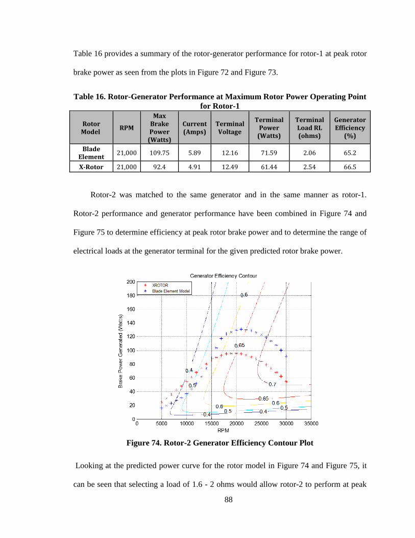
88

Table 16 provides a summary of the rotor-generator performance for rotor-1 at peak rotor

brake power as seen from the plots in Figure 72 and Figure 73.

Table 16. Rotor-Generator Performance at Maximum Rotor Power Operating Point

for Rotor-1

Rotor Model

RPM

Max Brake Power

(Watts)

Current (Amps)

Terminal Voltage

Terminal Power

(Watts)

Terminal Load RL (ohms)

Generator Efficiency

(%)

Blade Element

21,000 109.75 5.89 12.16 71.59 2.06 65.2

X-Rotor 21,000 92.4 4.91 12.49 61.44 2.54 66.5

Rotor-2 was matched to the same generator and in the same manner as rotor-1.

Rotor-2 performance and generator performance have been combined in Figure 74 and

Figure 75 to determine efficiency at peak rotor brake power and to determine the range of

electrical loads at the generator terminal for the given predicted rotor brake power.

Figure 74. Rotor-2 Generator Efficiency Contour Plot

Looking at the predicted power curve for the rotor model in Figure 74 and Figure 75, it

can be seen that selecting a load of 1.6 - 2 ohms would allow rotor-2 to perform at peak

89

power of 131 watts at 63% efficiency. At a load of 5 ohms, the rotor would produce less

power at a higher generator efficiency (100 watts @ 72% efficiency). Although higher

efficiencies are experienced while operating at 5 ohms, terminal power output is higher

with a load of 2 ohms by approximately 10 watts.

Figure 75. Rotor Brake Torque and Power Curves Overlaid Generator Brake


90

Table 17 provides a summary of the rotor-generator performance at peak rotor brake

power for rotor-2, as seen from the plots in Figure 74 and Figure 75.

Table 17. Rotor-Generator Performance at Max Rotor Power Operating Point for

Rotor-2

Rotor Model

RPM

Max Shaft Pwr

(Watts)

Current (Amps)

Terminal Voltage

Terminal Pwr

(Watts)

Terminal Load

(ohms)


(%)

Blade Element

Model 21000 130.9 7.07 11.7 83.1 1.66 63.5

X-Rotor 19000 95.8 5.67 10.72 60.8 1.89 63.5

Comparing how rotor-1 and rotor-2 match with the generator, rotor-1 is slightly a better

match by about 2-3 percent efficiency. Generally a rotor with untwisted blades generates

less brake power than a rotor with twisted blades however if the operating peak of the

lower performing rotor lies in a higher generator efficiency region than the higher

performing rotor, it is possible for the rotor that generates less brake power (Untwisted)

to produce a higher terminal electrical power output than the higher performing rotor.

Both rotors matched in this thesis operate at an acceptable efficiencies for the purpose of

model evaluation testing.

Following baseline rotor/generator matching, an example of a different generator

matched to rotor-1 will be presented. For the purpose of distinguishing between

generators, the generator previously matched to the baseline rotors will be referred to as

“Generator-A”, and the generator to be matched in this example as “Generator-B”. The

generator matched in this example is the BLDC Maxon generator #386678, shown in

Figure 76.

91

Figure 76. Generator-B Manufacturer Specifications [Maxon #386678] [18]

Parameters for both generators A and B are shown and compared below in Table 18.

Here we see that the Kv for generator-B is just over half of that of generator-A; with a

lower Kv the generators internal resistance and inductance reactance is higher. The

following Figure 77 andFigure 78 show the same type of plots produced for baseline

generator matching only now rotor-1 is being matched to generator-B.

Table 18. Generator A and B Manufacturer Specifications

Parameters Generator-A Generator-B

Kv [rpm/V] 1230 672

Ri [Ohms] 0.269 0.797

Io [Amps] 0.263 0.153

L [H] 0.000035 0.000118

92

Figure 77. Rotor-1 & Generator B Efficiency Contour

The region of max efficiency for generator-B is at about 75% beginning at a velocity of

approximately 26,000 rpm and brake power of about 50 watts. Rotor peak predicted

performance lies in the 70-72% efficiency region. It can be seen that generator-B is

slightly a better match then generator-A by about 5% efficiency at peak rotor operating

point.

93

Figure 78. Rotor-1 Brake Torque and Power Curves Overlaid Generator-B Brake


Now looking at the predicted power curve for rotor-1 plotted over generator-B

performance plots in both Figure 77 and Figure 78, it can be seen that selecting a load of

7.6 ohms would allow the rotor to perform at peak power of 109 watts at 71% efficiency.

At a load of 20 ohms, the blade would produce less power at a higher generator

efficiency (70 watts @ 75% efficiency). Although higher efficiencies are experienced

while operating at 20 ohms, terminal power output is higher with a load of 7.6 ohms by

94

approximately 12 watts. Table 19 provides a summary of the rotor-generator performance

at peak rotor brake power for rotor-1, as seen from the plots in Figure 77 and Figure 78.

Table 19. Generator-B Efficiency at Maximum Rotor-1 Power Operating Point

Rotor Model

RPM

Max Brake Power

(Watts)

Current (Amps)

Terminal Voltage

Terminal Power

(Watts)

Terminal Load

(ohms)


(%)

Blade Element

21000 109.75 3.2 24.35 78.11 7.6 71.2

X-Rotor 21000 92.4 2.7 24.9 66.7 9.3 72.2

Although generator-B is a slightly better match for rotor-1 than generator-A, it is not

a perfect match. A more better match would be if the rotor-1 peak brake power occurred

at or above a speed of about 26,000 rpm, closer to the maximum generator efficiency

point or alternatively if generator-B maximum efficiency occurred at the rotor-1 peak

brake power speed of 21,000 rpm. For selecting an electrical load for the generator, the

general trend suggest that for low speeds a higher resistance will result in lower power

generation and lower efficiencies and for high speeds a higher resistance will result in

higher power generated and higher efficiencies. In selecting a generator to match to a

rotor, it is important to understand how parameters effect performance. It is clear that

anything that contributes to losses such as resistance, inductance reactance, no-load

current, and rectifier losses will decrease generator maximum efficiency. Kv generally

affects the speed at which maximum efficiency occurs. For high Kv electrical machines,

max efficiency will occur at higher speeds than low Kv electrical machines.

Understanding how internal resistance and inductance trend with Kv also aids in the

selection of an appropriate generator. High Kv machines operate at relatively higher

speeds and lower torque; have thicker wire and fewer windings, resulting in lower

internal resistance and low inductance reactance. Lower Kv machines operate at

95

relatively higher torque, lower speeds and have thinner wire with more windings

resulting in higher internal resistance and higher inductance reactance. Based on this,

rotors that perform at relatively low speeds will match better with a low Kv generator and

rotors operating at high speeds will match better with a high Kv generator. A better match

for the baseline rotors 1 & 2 would be a generator of lower Kv compared to the baseline

generator Kv of 1230. However, the baseline rotor generator combination selected for

this thesis performs at a sufficient level for conducting model evaluation test.

96

5. BASELINE ROTOR/GENERATOR VALIDATION TEST

Baseline rotor/generator validation test have been conducted to evaluate both

generator and rotor design tools. Leading up to testing, both rotor and generator models

were implemented in determining rotor design and in matching the rotor to an off-the-

shelf brushless DC motor used as a generator. Through rotor/generator matching,

generator efficiency was assessed for the range of speeds and loads over which the rotor

operates. With confidence in the generator model established through motored-generator

testing described in Chapter 2.6 and the candidate validation rotor designed and matched

to a generator, the assembly and wind tunnel testing of the turbine generator was

conducted. This involved designing and manufacturing the candidate validation rotors, a

rotor/generator adapter, generator housing and a test stand to support the turbine-

generator assembly in the Cal Poly 2x2 ft. wind tunnel. Testing was then conducted with

varying electrical loads at wind tunnel speeds up to 110 mph. Results were then

compared to rotor and generator model predictions. Based on the comparison of test

results and model predicted performance, sources of discrepancy are assessed so that the

models can be modified to more closely predict performance.

5.1 Apparatus Design and Development

Following baseline rotor/generator matching and leading up to wind tunnel

evaluation testing, turbine components were designed and manufactured. Components

included the candidate baseline rotors, rotor/generator adapter, generator housing, Maxon

97

generator, and test stand. The exploded view of the complete turbine assembly is

illustrated in Figure 79.

Figure 79. Turbine Generator Assembly

5.1.1 Rotor

The geometry for the two-candidate rotor designs were previously presented in

Chapter 3.2 and have been referred to as rotor-1 and rotor-2. Geometry for these rotors

can be seen in Table 15 and Figure 52. In designing the rotors, previous rotor design

work was used as a starting point. Similar to previous designs, the rotor was designed

with a hollow space within the hub where the rotor/generator adapter could fit. The rotor

was then secured to the adapter with a 3 mm screw that went in through the tip of the hub

then screwing into the adapter. The hub diameter is 25.4 mm (1 inch) and was based on

the generator diameter (22 mm) and the wall thickness of the generator housing face

98

(2x1.7mm) which makes the generator housing face approximately equal to the hub

diameter. As mentioned before, because our rotor analysis tools are more accurate for a

low solidity rotor it was decided to design a rotor with three blades, equally spaced at

120° apart. Rotor solidity refers to the ratio of total blade area over the total swept area. A

high solidity rotor would be considered at a solidity of about 0.8, for this rotor the goal

was to maintain a solidity below 0.5.

99

5.1.2 Rotor/Generator Adapter

The rotor/generator adapter, shown below in Figure 80, is the device that couples

the rotor to the generator shaft. The adapter has a diameter of 14 mm that fits into an

equally sized cavity in the rotor hub and has a flange that provides a seat for the rotor hub

that extends out to a 20 mm diameter. At the bottom of the adapter, a 4 mm hole with a

depth of 6 mm allows the generator shaft to be secured to the adapter with the use of two

3 mm set screws. At the top of the adapter there is a 3 mm tapped hole that allows a

screw going through the tip of the rotor hub to be secured to the adapter. With the

tightening of the top screw and the tight fit between the adapter and the hub, the rotor

does not slip about the adapter.

Figure 80. Rotor/Generator Adapter

100

5.1.3 Generator Housing

The generator housing design was a modification of an original design by Schab

[26] who contributed to previous µRAT testing. The housing is composed of two parts,

front and aft, the front part of the generator housing is where the generator is enclosed

and attaches to the housing with three 2 mm screws at the face. The aft part of the

housing attaches to the front part of the housing and has a slot that mounts onto the test

stand and is secured with two screws. A half-inch diameter opening at the underside of

the aft housing allows the generator wires to exit the generator housing.

Figure 81. Front part of generator housing

Figure 82. Aft part of generator housing [26]

101

5.1.4 Test Stand

The Test Stand of Figure 83 is what holds the turbine at the center of the Cal Poly

2x2 ft. wind tunnel. Two cross bars attach to the wind tunnel bottom plate. The turbine

mounting point is at the top of a vertical bar that is supported by two cross-bars, 2

forward bracing bars, and L-brackets assembled as shown in Figure 83. This test stand

was reused from previous work [26].

Figure 83. Test Stand Attached to Bottom Wind Tunnel Plate [26]

Figure 84 displays the generator assembly attached to the Test Stand which is secured

onto the wind tunnel bottom plate. It can be seen that the turbine is cantilevered onto the

mounting bar of the test stand and is parallel to the wind tunnel bottom plate.

Figure 84. Turbine Generator Mounted on Test Stand [26]

102

5.2 Validation Test Results

The turbine generator validation test was conducted in the Cal Poly 2x2 ft, wind

tunnel at speeds ranging from about 71-110 mph; a schematic of the setup is displayed in

Figure 85. Starting from the left side of the diagram, the air flow is provided by the wind

tunnel which turns the wind turbine. The wind turbine produces AC power which is

rectified to DC power through the 3-phase bridge rectifier. Direct current then flows

through an electrical load (resistor bank) where terminal voltage and current are

measured. Axial airflow is measured by measuring differential pressure between

upstream and downstream contraction static pressure rings; this method of measuring

airspeed was selected over using a pitot tube in order to avoid any interference with

airflow directly in front of the rotor. RPM was determined by measuring the frequency

from one of the generator lead wires. The test setup represented in the schematic of

Figure 85 is shown in Figure 86.

Figure 85. Turbine Generator Validation Test Schematic [26]

103

Figure 86. Rotor/Generator Test Setup

Table 20 gives the contraction pressure coefficients obtained from an empty wind

tunnel calibration. This wind tunnel contraction calibration data is used to determine axial

air speed at the tunnel reference location in the center of the cross-section and 1 ft

downstream of the contraction exit by using the 𝐶𝑝,𝑛 value that corresponds to the

measured differential pressure then through Equation 69, reference dynamic pressure, q,

is solved for and axial flow velocity is calculated from q.

Table 20. Differential Pressures and Pressure Coefficients across the Wind Tunnel

Nozzle

Blower

motor

frequency

20 Hz 30 Hz 40 Hz 50 Hz 60 Hz

ΔPn (Pa) 151.546 351.514 631.067 985.495 1403.740

Cp,n 1.0025 0.9989 0.9899 0.987 0.9842

𝐶𝑝,𝑛 =

𝛥𝑃𝑛𝑞𝑟𝑒𝑓

(68)

𝑞𝑟𝑒𝑓 =

𝛥𝑃𝑛𝐶𝑝,𝑛

(69)

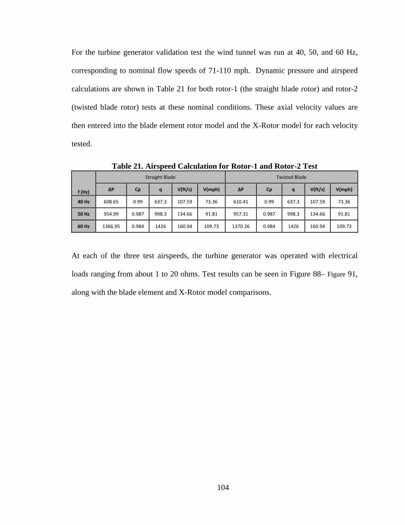
104

For the turbine generator validation test the wind tunnel was run at 40, 50, and 60 Hz,

corresponding to nominal flow speeds of 71-110 mph. Dynamic pressure and airspeed

calculations are shown in Table 21 for both rotor-1 (the straight blade rotor) and rotor-2

(twisted blade rotor) tests at these nominal conditions. These axial velocity values are

then entered into the blade element rotor model and the X-Rotor model for each velocity

tested.

Table 21. Airspeed Calculation for Rotor-1 and Rotor-2 Test

f (Hz)

Straight Blade Twisted Blade

ΔP Cp q V(ft/s) V(mph) ΔP Cp q V(ft/s) V(mph)

40 Hz 608.65 0.99 637.3 107.59 73.36 610.41 0.99 637.3 107.59 73.36

50 Hz 954.99 0.987 998.3 134.66 91.81 957.31 0.987 998.3 134.66 91.81

60 Hz 1366.95 0.984 1426 160.94 109.73 1370.26 0.984 1426 160.94 109.73

At each of the three test airspeeds, the turbine generator was operated with electrical

loads ranging from about 1 to 20 ohms. Test results can be seen in Figure 88– Figure 91,

along with the blade element and X-Rotor model comparisons.

105

Figure 87. Rotor-1 Power @ 49.05m/s compared to model predictions

Figure 88. Rotor 2 Power @ 49.05m/s compared to model predictions

0

10

20

30

40

50

60

70

80

0 5000 10000 15000 20000 25000 30000 35000

Elec

tric

al P

OW

ER (

WA

TTS

)

RPM

Rotor-1 (Straight Blades) POWER @ 60 Hz (UO=49.05 m/s)

Blade Element Model

X-Rotor

Actual_Power

0

10

20

30

40

50

60

70

80

90

0 5000 10000 15000 20000 25000 30000 35000

ELEC

TRIC

AL

PO

WER

(W

AT

TS)

RPM

ROTOR 2 (Twisted Blades) POWER @ 60 Hz (Uo=49.05 m/s)

Blade Element Model

X-Rotor

Actual Power

106


Figure 90. Rotor 2 Power @ 41.04m/s compared to model predictions

0

5

10

15

20

25

30

35

40

45

0 5000 10000 15000 20000 25000 30000

ELEC

TRIC

AL

PO

WER

(W

AT

TS)

RPM

Rotor-1 (Straight Blades) POWER @ 50Hz (Uo=41.04 m/s)Blade Element Model

X-Rotor

Actual_Power

0

10

20

30

40

50

60

0 5000 10000 15000 20000 25000 30000 35000

ELEC

TRIC

AL

PO

WER

(W

AT

TS)

RPM

Rotor-2 (Twisted Blades) POWER @ 50 Hz (Uo=41.044 m/s)Blade Element ModelX-RotorActual Power

107

Figure 91. Rotor-1 Power @ 32.79 m/s compared to model predictions


0

5

10

15

20

25

0 5000 10000 15000 20000 25000

ELEC

TRIC

AL

PO

WER

(W

AT

TS)

RPM

Rotor-1 (Straight Blades) POWER @ 40 Hz (Uo=32.79 m/s)Blade Element ModelX-RotorActual_Power

0

5

10

15

20

25

0 5000 10000 15000 20000 25000

ELEC

TRIC

AL

PO

WER

(W

AT

TS)

RPM

ROTOR-2 (Twisted Blades) POWER @ 40 Hz (Uo=49.05 m/s)Blade Element ModelX-RotorActual Power

108

5.3 Discussion

It can be seen that the measured and predicted results for generated power seem to

follow similar trends, but the measured power output is significantly lower than predicted

by either the blade element or X-Rotor/ generator models. Generally, the measured

power at peak power was observed to be 20-30% lower than predicted by X-Rotor

combined with the proposed generator model for both rotor-1 and rotor-2; the blade

element model in combination with the proposed generator model predicts significantly

higher at about 50% higher for rotor-1 and up to 75% higher for rotor-2. Additionally, it

was observed that rotor-1’s measured peak power occurred at a higher RPM than

predicted, whereas the RPM for peak power predicted for rotor-2 (twisted-blade) occurs

at about the same value that was predicted. Some of the differences between predicted

and measured power may be attributed to the accuracy of the generator model, and in

particular to the prediction of generator shaft torque. However, based on the earlier

motor-driven generator test results, it is believed that most of the discrepancy is due to

inaccuracy in the rotor performance modelling. For example, both rotor models require

lift/drag data which is crudely modelled—especially for stalled blades—and, aero-elastic

deformation of the rotor blades is not included in the model. In addition, no attempt has

yet been made to include induced flow and finite span effects in the blade element model;

these influences are expected to make its predictions too high for maximum power. It is

therefore concluded that the proposed generator model is probably sufficient although a

direct torque measurement would be desirable; further development of the µRAT design

tools should focus on an improved rotor performance model. The possibility that aero-

elastic deformation could be part of the reason for the over-prediction of the power could

109

be tested by fabricating and testing a stiffer (metal) rotor with the same geometry as one

of the rotors tested here.

5.4 Rotor Model Tip Loss Corrections

At this point it was decided to examine whether the lack of inclusion of induced flow

effects was indeed responsible for the large difference between the blade element rotor

model and X-Rotor predictions. As previously mentioned, the blade element rotor model

does not account for Induced flow effects associated with an airfoil of finite aspect ratio.

At the blade tips, bounded vortices that lie along the span of an airfoil will cause air to

flow around the tip of the blade resulting in low lift generation at the blade tip. The

current blade element model uses simple 2-D airfoil data and therefore calculates

substantial lift generated at the blade tip. The Prandtl tip loss model provides a simple

and easy-to-implement approximate treatment of this effect and in effort to account for

the losses at the blade tip due to wing tip vortices the Prandtl tip loss corrections have

been implemented in the blade element model. Prandtl’s factor (𝐹𝑝) is defined below in

Equation 70

𝐹𝑝 =2

𝜋 𝑎𝑟𝑐 cos 𝑒−𝑓 (70)

Where

𝑓 =𝐵

2 𝑅 − 𝑟

𝑟 sin∅ (71)

For the expression for 𝑓, B represents the number of blades, R, is the blade outer radius,

r, represents the local radius of each element and ∅ is the relative velocity angle. Figure

110

93 shows the Prandtl tip loss factor as a function of normalized radius for rotor-2 at peak-

generated power at an airspeed of 110 mph.

Figure 93. Prandtl Tip Loss Factor (Fp) as a Function of Normalized Radius

In implementing this factor, sectional thrust and torque equations presented in chapter 3.2

are modified (Equations 63 and 64). Below the Prandtl factor has been applied to both

equations.

∆𝑇 = 𝐹𝑝 ∗ 𝜌4𝜋𝑟𝑉∞2𝑎(1 + 𝑎)∆𝑟 (72)

∆𝑄 = 𝐹𝑝 ∗ 𝜌4𝜋𝑟3𝑉∞𝑏(1 + 𝑎)𝜔∆𝑟 (73)

The difference in coefficient of lift along the rotor blade, with and without the tip loss

factor can be seen in Figure 94 and Figure 95 for rotor-2 at peak-generated power at an

airspeed of 110 mph. Here we see how the sectional torque with the factor applied more

0.4 0.5 0.6 0.7 0.8 0.9 10.2

0.3

0.4

0.5

0.6

0.7

0.8

0.9

1

Prndtl Tip Loss Factor

R/r

Fp

111

closely models the effects of tip losses with the sectional torque approaching zero closer

to the tip of the blade.

Figure 94. Sectional Torque without Tip Loss Factor

Figure 95. Sectional Torque with Tip Loss Factor

0.4 0.5 0.6 0.7 0.8 0.9 1

-0.004

-0.0035

-0.003

-0.0025

-0.002

-0.0015

-0.001

-0.0005

Sectional Torque

R/r

Torq

ue [

ft-lb]

0.4 0.5 0.6 0.7 0.8 0.9 1

-0.0024

-0.0022

-0.002

-0.0018

-0.0016

-0.0014

-0.0012

-0.001

-0.0008

Sectional Torque

R/r

Torq

ue [

ft-lb]

112

The following figures apply the Prandtl tip loss factor to the blade element model for the

same flight conditions and for the same baseline rotors as in the model evaluation test in

Chapter 5.2. Here we see that the blade element rotor model with the Prandtl tip loss

factor applied generally predicts a significantly lower generated power – much closer to

X-Rotor results than the rotor model without the tip loss factor. Looking at predictions

for rotor-1 at all three speeds, peak power between the blade element model with tip-loss

comes within about 1.5% difference of X-Rotor at approximately the same speeds. Peak

power for the blade element rotor model is shifted to the right of X-Rotor peak power by

about 1,000 rpm. For rotor-2 at all three speeds, peak power between the blade element

model with tip-loss comes within about 5-8% difference of X-Rotor at similar speeds.

Just like in the case for rotor-1, for rotor-2 the peak power for the blade element rotor

model is shifted to the right of X-Rotor peak power by about 1,000 rpm. Looking at

model comparisons to actual measured results Figure 96 and Figure 101 ) it is apparent

that the blade element model with Prandtl tip-loss effects more closely models flow

experienced by the actual rotor and the predicted power results compare closely to X-

Rotor results. Applying this factor brings predictions with the blade element model from

50-75 % error to within 25-40% error of blade evaluation test results. For these reasons

the Prandtl tip loss factor, or perhaps a more sophisticated model to account for induced

flow effects, should be incorporated in the blade element model.

113


Figure 97. Rotor-2 Power @ 49.05m/s Compared to Model Predictions

0

10

20

30

40

50

60

70

80

0 5000 10000 15000 20000 25000 30000 35000

Elec

tric

al P

OW

ER (

WA

TTS

)

RPM

Rotor-1 (Straight Blades) POWER @ 60 Hz (UO=49.05 m/s)Blade Element Model

X-Rotor

Actual_Power

Blade Element Model w/Prandtl TipLoss

0

10

20

30

40

50

60

70

80

90

0 5000 10000 15000 20000 25000 30000 35000

ELEC

TRIC

AL

PO

WER

(W

AT

TS)

RPM

Rotor-1 POWER @ 60 Hz (UO=49.05 m/s)Blade Element Model

X-Rotor

Actual Power

Blade Element Model w/Tip Loss

114



0

5

10

15

20

25

30

35

40

45

0 5000 10000 15000 20000 25000 30000

ELEC

TRIC

AL

PO

WER

(W

AT

TS)

RPM

Rotor-1 (Straight Blades) POWER @ 50 Hz (Uo=41.04 m/s)Blade Element Model

X-Rotor

Actual_Power


0

10

20

30

40

50

60

0 5000 10000 15000 20000 25000 30000 35000

ELEC

TRIC

AL

PO

WER

(W

AT

TS)

RPM

Rotor-2 (Twisted Blades) POWER @ 50 Hz (Uo=41.04 m/s)Blade Element Model

X-Rotor

Actual Power

Blade Element Model w/ Tip Loss

115

Figure 100. Rotor-1 Power @ 32.79 m/s Compared to Model Predictions


0

5

10

15

20

25

0 5000 10000 15000 20000 25000

ELEC

TRIC

AL

PO

WER

(W

AT

TS)

RPM

Rotor-1 (Straight Blades) POWER @ 40 Hz (Uo=32.79 m/s)Blade Element Model

X-Rotor

Actual_Power


0

5

10

15

20

25

0 5000 10000 15000 20000 25000

ELEC

TRIC

AL

PO

WER

(W

AT

TS)

RPM

ROTOR-2 (Twisted Blades) POWER @ 40 Hz (Uo=32.79 m/s)Blade Element Model

X-Rotor

Actual Power

Blade Element Model w/Prandtl Tip Loss

116

6. CONCLUSION AND RECOMMENDATIONS

This thesis project was undertaken to assemble a set of design tools to be employed

for the design of a µRAT for specific operating conditions. The µRAT design tools

developed consist of turbine rotor and generator models. The primary focus of this thesis

was in developing the generator model which can be used to predict the performance of a

brushless DC machine operated as a generator. The generator model presented is able to

predict generator brake power and output electrical power with and without rectification

as a function of shaft speed and electrical load with only basic manufacturer

specifications given as inputs. Initially it was a challenge to account for all power losses,

however, through model evaluation testing and in comparisons between measured and

predicted results it became clear that it was necessary to account for generator no-load

current, internal resistance, inductance reactance, terminal load resistance, and rectifier

losses. The finalized generator model was then able to predict performance to within a

few percent error.

For the turbine rotor model, momentum and basic, 2-D, blade element theory was

implemented in conducting rotor performance analysis and geometry selection. Rotor

model results were expected to over-predict rotor torque and power due to the model not

taking into account induced flow effects. A second model, X-Rotor, that includes induced

flow was then used to predict power and for comparison to the rotor model results. Rotor

models were then evaluated through wind tunnel validation test conducted on a turbine

generator with two different rotors, rotor-1 (untwisted blades) and rotor-2 (twisted

blades). Results indicated power predictions to be 50-75% higher for the blade model and

117

20-30% higher for Xrotor. It was assessed that induced flow effects along with aero-

elastic deformation are likely contributors to error between model results and measured

values. In effort to approximately account for some of the induced flow effects in the

rotor model, the Prandtl tip-loss factor was implemented in the rotor model. With the tip-

loss factor implemented in the rotor model, predictions were much closer to X-Rotor

results and about 20-40% higher than actual results.

Some of the conclusions that have been established throughout this project include

various aspects of the approach taken in characterizing rotor and generator performance

and in the methods of model evaluation.

These conclusions are as follows:

1. A model of the performance of a brushless DC machine operated as a generator has

been developed that uses readily-available manufacturer specified machine parameters

such as internal resistance (𝑅𝑖), no-load Current (𝐼𝑜), Speed Constant (𝐾𝑉) and Inductance

(L), and includes rectification of its output if desired.

2. Losses in the generator model due to the rectifier are significant and should not be

neglected. For example, the difference between including and excluding rectifier losses in

the generator model for the Maxon generator #386677 operating with a 5-ohm load at

30,000 rpm is about 7.25%.

3. Based on the motor-driven generator test results, it is believed that most of the

discrepancy in baseline rotor/generator validation test between predicted and observed

power generated is due to inaccuracy in the rotor performance modelling and is

concluded that the proposed generator model is probably sufficient although direct torque

measurements are desired.

118

4. Motor/generator specifications provided by the manufacturer do not necessarily

match the values that are published and do not necessarily remain constant with speed.

For the Maxon motor actual Kv and Ri, values were within 0.5% percent error from what

was published. However, for the Ammo motor that was used in the motored generator

test, Kv values had a 38% error and the no-load current was not a constant 1.9 Amps, as

published, and varied significantly with speed.

5. Rotors that perform at relatively low speeds will match better with a low Kv

generator and rotors operating at high speeds will match better with a high Kv generator.

6. The RPM measurement method of reading the frequency from one of the generators

lead wires is most accurate above 8,000 RPM. Measurements taken below this value tend

to be noisy and not as reliable.

7. Cogging in motor/generators is torque that stems from the interaction between the

permanent magnets and the teeth of the rotor/stator that follows the trend depicted in

Figure 16. For the generator it is an undesirable characteristic since cogging will require a

higher cut in torque from the blades and cause velocity and torque ripples. For evaluating

generator results, velocity and torque ripples are not desired due to resulting power wave

distortion that is not accounted for in the generator model.

8. Blade element rotor model predictions are significantly higher than actual results

due to the model not accounting for 3-D flow effects. Applying the Prandtl tip loss factor

to the rotor model accounts for some of these losses associated with the flow at the blade

tip. Applying this factor brings predictions with the blade element model from 50-75 %

error to within 25-30% error compared with experimental measurements for the baseline

rotor tests.

119

Based on the results and conclusions of this project, the following are the

recommendations for future work:

Further development of the µRAT design tools should focus on an improved

rotor performance model.

If desired, direct torque measurements with a torque transducer or torque

cradle should be undertaken to more thoroughly evaluate the generator

model. However, model evaluation conducted in this thesis should be

sufficient.

Rectifier losses should always be accounted for in the generator model. To

minimize rectifier losses, Schottky rectifiers could be considered.

Motor/generator published specifications should be used in rotor/generator

matching. However, Once the generator is in hand, generator performance

specifications should always be verified using the methods in Chapter 2.5.

For model evaluation test for a rotor/generator that operates below or near

8,000 RPM an alternate method for accurately reading RPM than the one

used in this thesis should be investigated.

Although matching a generator to a rotor may be an iterative method as

suggested by Figure 69, initial selection of a generator to be matched to a

rotor should be based on the Kv parameter; High Kv for high speed

operating rotor and low Kv for low speed operating rotor.

Generators with cogging torque should be avoided. If unavoidable, it will be

required that the blade cut-in torque overcomes both the cogging torque

along with the no-load torque.

120

The Prandtl tip loss factor should be incorporated in the blade element

model.

121

REFERENCES

[1] R. V. Westphal, Interviewee, The Boundary Layer Data System. [Interview].

22014-2015.

[2] H. H. Oo, Interviewee, 2mm Foil Scrim Pyrogel Insulation in Still Air and Wind

Tunnel Test. [Interview]. Jun-Jul 2014.

[3] Woodbank Communications Ltd, "Electrical Machines - Electric Drives

(Fundamentals)," 2005. [Online]. Available:

http://www.mpoweruk.com/machines.htm. [Accessed Jan 2015].

[4] S. J. Chapman, Electric Machinery Fundamentals, New York, NY: McGrawHill,

2005.

[5] "Electric Meters & Motors," [Online]. Available:

http://boomeria.org/physicslectures/secondsemester/electricity/metersmotors/mete

rsmotors.html. [Accessed Jan 2015].

[6] "Working Principal of DC Motor," 2013. [Online]. Available:

http://workingprincipalofdcmotor.blogspot.com/. [Accessed Jan 2015].

[7] J. Hauge, D. Hutcheson and P. "Scott", "Boundary Layer Data System (BLDS)

Heating System," San Luis Obispo, 2009.

122

[8] M. Drela, "DC Motor / Propeller Matching Lab 5 Lecture Notes," 03 Mar 2005.

[Online]. Available: http://web.mit.edu/drela/Public/web/qprop/motorprop.pdf.

[Accessed 1-30 Jun-Jul 2015].

[9] D. Wood, Small Wind Turbines Analysis, Design, and Application, Calgary:

Springer, 2011.

[10] Centurion Energy, Alternative Energy, "Types of Wind Turbines," 2013.

[11] H. Glauert, The Elements of Aerofoil and Airscrew Theory, vol. 2nd ed, New

York, NY: Cambridge University Press, 1947.

[12] D. J. Auld, "Aerodynamics for Students, Analysis of Propellers," AMME,

University of Sydney, 1996-2006. [Online]. Available: http://www-

mdp.eng.cam.ac.uk/web/library/enginfo/aerothermal_dvd_only/aero/propeller/pr

op1.html. [Accessed May-Jun 2015].

[13] J. F. Manwell, J. G. McGowan and A. L. Rogers, Wind Energy Explained

Theory, Design and Application, Chichester, West Sussex: John Wiley & Sons

Ltd., 2009.

[14] Maxon Motor ag, "Motor Data and Operating Ranges of Maxon DC Motors,"

Maxon Motors, 2010. [Online]. Available: www.maxonmotor.com/academy.

[Accessed 29 1 2015].

123

[15] W. Storr, "Basic Electronics Tutorial," 2 2 2015. [Online]. Available:

http://www.electronics-tutorials.ws/inductor/ac-inductors.html . [Accessed 2 2

2015].

[16] Z. Q. Zhu and D. Howe, "Influence of Design Parameters on Cogging Torque in

Permanent Magnet Machines," IEEE Transations on energy conversion, vol. 15,

no. 4, pp. 1-5, 2000.

[17] The Electric Energy, "What is a Brushless DC Electric Motor," [Online].

Available: http://theelectricenergy.com/what-is-a-brushless-dc-electric-motor/ .

[Accessed 29 1 2015].

[18] M. Motor, "Maxon Motor usa," [Online]. Available:

http://www.maxonmotorusa.com/maxon/view/content/index. [Accessed Jan

2015].

[19] OpenWetWare, "Diodes," [Online]. Available:

http://openwetware.org/wiki/20.309:DiodePrimer . [Accessed 29 1 2015].

[20] MarineInsight, "Understanding Rectifier and Rectifier Circuits," [Online].

Available: http://www.marineinsight.com/tech/marine-electrical/uses-of-

rectifier-and-rectifier-circuits-on-ship/.

[21] IXYS, Three Phase Rectifier Bridge FUO22-12N, 2007.

[22] M. Drela and H. Youngren, "XROTOR User Guide," MIT, 2003.

124

[23] D. Marten and J. Wendler, "QBlade Guidelines v0.6," tu-berlin, 2013.

[24] M. Drela and H. Youngren, "XFOIL Subsonic Airfoil Development System,"

MIT, 11 December 2000. [Online]. Available:

http://web.mit.edu/drela/Public/web/xfoil/. [Accessed Jun-Dec 2014].

[25] B. Montgomerie, "Methods for Root Effects, Tip Effects and Extending the

Angle of Attack Range to ±180°, with Application to Aerodynamics for Blades

on Wind Turbines and Propellers," FOI - Swedish Defence Research Agency,

2004.

[26] B. Schab, MicroRAT Test; Shrouded and Un-Shrouded Turbine Performance

Comparison, San Luis Obispo, CA, 2010.

125

APPENDICES

APPENDIX A. ROTOR MODEL MATLAB

% Glauert Blade Element Theory

B = 3; %Number of Blades %INITIAL GUESS FOR alpha

%FLIGHT CONDITIONS Vinf=161.333; % Upstream Airspeed [ft/s] rho=0.002377; % Density [slug/ft^3]

%AIRFOIL DATA READER old=cd('D:\Thesis\CODE\DATA'); filename='naca2412_RE80.txt'; % FoilData=readr2(filename); cd(old);

%DISK DIMENSIONS [INPUT] %********************************************* Do= 3.25; % Rotor Outer Diameter [in] Di= 25.4/25.4; % Rotor Hub Diameter [in] %*********************************************

Do_ft=Do/12; % [ft] Di_ft=Di/12; % [ft] Dan=Do-Di; % Annular Diameter [in] Dan_ft=Dan/12; % [ft]

ro= Do/2; % Rotor Outer Radius [in] ri= Di/2; % Roter Hub Radius [in] ro_ft=ro/12; % [ft] ri_ft=ri/12; % [ft] ran=ro-ri; % Annular Radius [in] ran_ft=ran/12; % [ft]

%EFFECTIVE RADIUS CORRECTION FACTOR [INPUT] Rcf=1; % Effective Correction Factor Reff=ri_ft+Rcf*ran_ft; Reffan=Reff-ri;

%BLADE ELEMENTS [INPUT] N=20; % Number of Elements dr=ran_ft/N;

126

%DEFINES RADIUS AT THE MIDPOINT OF EACH ELEMENT for i=1:N+1 if i==1 r(i)=ri_ft+dr/2; end if i==N r(i)=ri_ft+(i-1)*dr+dr/2; end if i==(N+1) r(i)=r(N)+dr/2; end

if i>1 && i<N r(i)=ri_ft+(i-1)*dr+dr/2; end

end r_R=r(1:N)./ro_ft;

%**************************************************** % INPUT BLADE GEOMETRY ** [INPUT] %***************************** %PITCH TWIST ** Pt=-25; %deg ** %BLADE ANGLE at HUB ** Ph=40; %15deg ** %CHORD AT HUB ** Ch=0.511811/12;%[ft] ** %CHORD AT TIP ** Ct=1*Ch;%[ft] ** %***************************** %delta Chord dc=Ch-Ct;

%PITCH w/Blade Twist (Linear) theta_p=Ph+((r-ri_ft)./ran_ft).*Pt; % theta_p=Tgeo(:,3); % %PITCH (CONSTANT) ****Uncomment if Pitch is Constant and Comment out

^^ % theta_p=Ph;

%CHORD(FT) (Linear Taper starting from hub) c=Ch-((r-ri_ft)./ran_ft).*dc; % chord [ft] c_R=c./ro_ft;

%SOLIDITY AT EACH ELEMENT s=(B.*c)./(2*pi.*r);

%INITIAL GUESS FOR INFLOW FACTORS a(1,1)=-.1; b(1,1)=-.1; aold(1,1)=a(1,1);

127

bold(1,1)=b(1,1);

%ROTOR SPEED [INPUT] rpm=5000:1000:30000; rps=rpm./60;

W_relax=.5; for g=1:length(rpm); RPM=rpm(g); RPS=RPM/60; w=RPS*(2*pi); W(g)=w;

if g > 1 a(g,1)=a(g-1,1); b(g,1)=b(g-1,1); aold(g,1)=a(g,1); bold(g,1)=b(g,1); end %CALCULATES PARAMETERS FOR EACH ELEMENT for j=1:N if j>1 aold(g,j)=a(g,j-1); bold(g,j)=b(g,j-1); a(g,j)=a(g,j-1); b(g,j)=b(g,j-1); end

%ITERATES TO CONVERGE ON a & b % Max Iterations itermax = 250; % Tolerance for convergence tol = .0001; for i=1:itermax Vo(g,j) = Vinf*(1+a(g,j)); V2(g,j) = W(g)*r(j)*(1-b(g,j)); alpha(g,j) = theta_p(j)-atand(Vo(g,j)/V2(g,j)); phi(g,j) = theta_p(j)-alpha(g,j); V1(g,j) = sqrt(Vo(g,j)^2+V2(g,j)^2); Re(g,j) = (V1(g,j)*c(j))/0.00015723;

cl(g,j) = -interp1(FoilData.alpha,FoilData.CL,-

alpha(g,j)... ,'pchip'); cd(g,j) = (interp1(FoilData.alpha,FoilData.CD,-

alpha(g,j)... ,'pchip'));

%*****PRANDLT CORRECTION FACTOR****** f(g,j)=(B/2).*((ro_ft-r(j))/... (r(j)*sin(phi(g,j)*(pi/180)))); Fp(g,j)=(2/pi).*acos(exp(-f(g,j)));

128

dT_dr(g,j)=.5*rho*V1(g,j)^2*c(j)* (cl(g,j)... *cosd(phi(g,j))-cd(g,j)*sind(phi(g,j)))*B; dQ_dr(g,j)=.5*rho*V1(g,j)^2*c(j)* (cl(g,j)... *sind(phi(g,j))+cd(g,j)*cosd(phi(g,j)))*B*r(j); dT(g,j)=dT_dr(g,j)*dr; dQ(g,j)=dQ_dr(g,j)*dr;

L1(g,j)=dT_dr(g,j)/(Fp(g,j)*rho*4*pi*r(j)*Vinf^2*(1+a(g,j)));

L2(g,j)=dQ_dr(g,j)/(Fp(g,j)*rho*4*pi*r(j)^3*Vinf*(1+a(g,j))*w); a_new(g,j)=.5*(a(g,j)+L1(g,j)); b_new(g,j)=.5*(b(g,j)+L2(g,j)); a(g,j)=a_new(g,j); b(g,j)=b_new(g,j); % A(g,i,j)=a(g,j); A(g,j,i)=a(g,j); BB(g,j,i)=b(g,j);

%CONVERGING CRITERIA----------------------------------------

diffa(g,j) = abs(a(g,j)-aold(g,j)); diffb(g,j)= abs(b(g,j)-bold(g,j));

if (diffa(g,j) < tol) && (diffb(g,j) < tol)

break % Exit iteration loop because of

convergence

end

if i > 90 i A(g,j,i)=A(g,j,i)*W_relax+(1-W_relax)*A(g,j,i-1); BB(g,j,i)=BB(g,j,i)*W_relax+(1-W_relax)*BB(g,j,i-1); a(g,j)=A(g,j,i); b(g,j)=BB(g,j,i); end % Warning if the maximum # of iteration dteps was reached

without % convergeing if (i == itermax) disp('Warning: code did not converge'),disp(g),disp(j) end aold(g,j)=a(g,j); bold(g,j)=b(g,j);

end

end %Power dT_sum(g) = sum(dT(g,:)); dQ_sum(g) = sum(dQ(g,:)); dP(g)=sum(W(g).*dQ(g,:)*1/0.737562149);

129

end

figure(1) subplot(2,1,1) plot(rpm,dQ_sum,'*'),grid on,,xlabel('Rotor Speed w [rpm]')... ,ylabel('Torque [ft lbf]'),set(gca,'YDir','reverse'); set(gca, 'XTickLabel', get(gca, 'XTick')); subplot(2,1,2) plot(rpm,dP,'*'),grid on, grid on,,xlabel('Rotor Speed w [rpm]')... ,ylabel('Power [Watts]'),set(gca,'YDir','reverse'); set(gca, 'XTickLabel', get(gca, 'XTick'));

%% display for g=1:length(rpm) for j=1:N % A(j,1) = r_R(j); A(j,2) = Vo(g,j); A(j,3) = V2(g,j); A(j,4) = V1(g,j); A(j,5) = alpha(g,j); A(j,6) = phi(g,j); A(j,7) = a(g,j); A(j,8) = b(g,j); A(j,9) = s(j); A(j,10) = cl(g,j); A(j,11) = cd(g,j); A(j,12)= Re(g,j);

F(j,1) = dT(g,j); %Thrust F(j,2) = dQ(g,j); %Torque end %Power =Torque*w

F(:,3)=W(g).*F(:,2).*1/0.737562149; %Power F(1,4)=sum(F(:,2)); %sum of Trq F(1,5)=sum(F(:,1)); %sum of Thrust F(1,6)=sum(F(:,3)); %sum of Power

disp('@RPM'),disp(rpm(g)) disp(' r_R Vax(disk) Vang(disk) Vrel(disk)

alpha phi a b sol CL CD' ) disp('--------------------------------------------

----------------------------------------------------------------') disp(A(:,1:11))

disp(' dT dQ Power[watt] sum(Trq)

sum(Thrust) sum(Power[watt]) ') disp('---------------------------------------------

--------------------------------------') disp(F) end

130

APPENDIX B. GENERATOR MODEL MATLAB

%% GENERATOR PERFORMANCE FOR VARYING ELECTRICAL LOADS

clear all close all clc Rl=[2 4 6 8 10 20]; Ln={':','-','--','-'}; for j=1:length(Rl)

RL=Rl(j); %ohms1.74; P=2; %Number of Poles of the Generator Ri=.797; %Generator Internal Resistance Kv=672; %Generator Velocity Constant Io=0.153; %Average No Load Current (Io did not change much with

RPM)

RPM=0:100:35000;%RPM measured from Generator Lead wire RPS=RPM/60; w=RPS*(2*pi); f=(RPM*P)/(60*2); L=.000118;

%Rectifier Vf=1.1; % Approximate Voltage Drop per Diode Rd=.12; % Approximate Resistance per Diode Vdo=Vf*2; % Total Rectifier Voltage drop (2 Diodes on) Rdo=Rd*2; % Total Rectifier Resistance (2 Diodes on) Vthresh=Vdo; %Below Rectifier Threshold V_o=RPM./Kv; I=Io; %Below threshold Voltage no current flows through circuit Ps_o=V_o.*Io; Trq_o=Ps_o./w;

Va_p=RPM./Kv; %Single Phase Vpeak Va=Va_p./sqrt(2); %Single Phase Vrms Vr_p=Va_p-Vdo; %Vr_av=Vr_p/(pi/(2*sqrt(2))); I=Vr_p./(RL+Ri+(2*pi*f.*L)); Iav=I.*(3/pi); V=I.*RL; Vav=Iav.*RL; %Iav=Vr_av/RL; %I=(Va+Vdo)/(Ri+RL+Rdo);%Circuit Current

P=Iav.*Vav;

Ia=Io+I; %peak shaft power

131

Pshaft=Va_p.*Ia;

%Shaft Torque Trq=Pshaft./w; %efficiency (Peak Efficiency) eta=((Vav.*Iav)./Pshaft).*100; % %efficiency (Peak Efficiency) % eta=(Vav.*Iav)./Pshaft;

for i=1:length(RPM) if Va_p(i) < Vthresh TRQ(i)=Trq_o(i); PRW_s(i)=Ps_o(i); else TRQ(i)=Trq(i); PRW_s(i)=Pshaft(i); end if Ia(i) <= Io I(i)=0; V(i)=0; Pshaft(i)=0; eta(i)=0; else I(i)=I(i); end end figure (1) k = plot(RPM,TRQ),grid on,... title('Brake Torque for Different Electrical Loads (RL)')... ,xlabel('RPM'), ylabel('Brake Torque (N-m)') clabel([Rl(j) RPM;length(TRQ) TRQ],k) hold on set(gca, 'XTickLabel', get(gca, 'XTick')); ylim([0 0.1])

figure (2) hold on h = plot(RPM,PRW_s), grid on,... title('Brake Power for Different Electrical Loads (RL)')... ,xlabel('RPM'), ylabel('Brake Power (Watts)') clabel([Rl(j) RPM;length(PRW_s) PRW_s],h) set(gca, 'XTickLabel', get(gca, 'XTick')); ylim([0 200]) figure (3) v = plot(RPM,eta), grid on,... title('Generator Efficiency for Different Electrical Loads

(RL)')... ,xlabel('RPM'), ylabel('Generator Efficiency') clabel([Rl(j) RPM;length(eta) eta],v) hold on

132

B.1 Generator Model Efficiency Contour Charts

%% GENERATOR CONTOUR ***WORKING*** close all clear all clc

%GENERTOR PARAMETERS [INPUT] Kv=1230*((2*pi)/60); % Kv in (rad/s)/volt Ri=0.269; % Ohms Io=0.263; % Amps L=0.000035; % Inductance p=2; % # of Generator poles; [2 poles = 1 pole pair] %************* %RECTIFIER [INPUT] Vf=1.1; % Approximate Voltage Drop per Diode Vdo=Vf*2; % Total Rectifier Voltage drop (2 Diodes on) Vthresh=Vdo; %*************

% POWER AND SPEED INPUT RANGES PSHAFT=5:10:500; % Watts RPM=0:10:35000; % Revolutions per Minute

RPS=RPM./60; % Revolutions per Second W=RPS.*(2*pi); % Radians per Second [rpm, Pshaft] = meshgrid(RPM,PSHAFT); rps=rpm./60; w=rps.*(2*pi); f=(rpm.*p)./(60*2); % Frequency Vu_p=(w./Kv); % Peak Armature Voltage Vu=(w./Kv).*sqrt(2); % Armature Voltage Trq=Pshaft./w;

% RECTIFIER THRESHOLD VOLTAGE % *************************** V_o=RPM./Kv; I=Io; Ps_o=V_o.*Io; Trq_o=Ps_o./W;

%Below threshold Voltage no current flows through circuit for i=1:length(PSHAFT) for j=1:length(RPM) if Vu_p(i,j) < Vthresh Trq(i,j)=Trq_o(i); Pshaft(i,j)=Ps_o(i); else Trq(i,j)=Trq(i,j); Pshaft(i,j)=Pshaft(i,j); end

end

133

end %****************************

Iu=Pshaft./Vu_p; %Useful current

%disp('RPM'), disp (rpm) %disp('frequency (Hz)'), disp (f) % CURRENT [AMPS] I=Iu-Io; % Peak Current [AC Amps] I_av=I.*(3/pi); % Peak Current [DC Amps] %Voltage Drop V=Vu_p-I.*Ri-Vdo-I.*(2*pi.*f.*L);

%Below threshold Voltage no current flows through circuit for i=1:length(PSHAFT) for j=1:length(RPM) if Iu(i,j) <= Io I(i,j)=0; I_av(i,j)=0; V(i,j)=0; Pshaft(i,j)=0; eta(i,j)=0; else I(i)=I(i); end

end end

% Terminal Voltage [DCV] V_av=V.*(3/pi); % Terminal Power [Watts] P=I.*V; P_av=P.*(3/pi)^2; % [DC] %Resistive Load (Rl) R=V./I; %Efficiency eta=(P_av)./Pshaft; PP=V_av.*I_av;

% CONTOUR PLOTS figure(1) [CC,hh]=contour(rpm,Pshaft,eta,... [0.50 0.60 0.65 0.7 0.75 0.8 0.85 0.9 ]); clabel(CC,hh); xlabel('RPM'),grid on, ylabel('Brake Power (Watts)'),... title('Generator Efficiency Contour') axis([0 35000 0 200]) set(gca, 'XTickLabel', get(gca, 'XTick')); %axis([0 35000 0 150]) %xlim([0 RPM_top]) %ylim([0 200])

figure(2)

134

[CC,hh]=contour(rpm,(V_av.*I_av),eta,... [0.50 0.60 0.65 0.7 0.75 0.8 0.85 0.9 ]); clabel(CC,hh); xlabel('RPM'),grid on, ylabel('Terminal Power (Watts)'),... title('Generator Efficiency Contour') axis([0 35000 0 200]) set(gca, 'XTickLabel', get(gca, 'XTick')); %xlim([0 RPM_top]) %ylim([0 200])

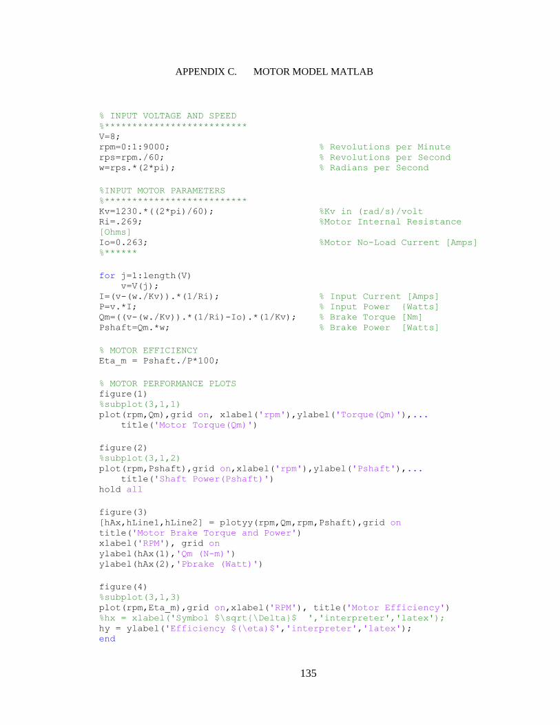
135

APPENDIX C. MOTOR MODEL MATLAB

% INPUT VOLTAGE AND SPEED %************************** V=8; rpm=0:1:9000; % Revolutions per Minute rps=rpm./60; % Revolutions per Second w=rps.*(2*pi); % Radians per Second

%INPUT MOTOR PARAMETERS %************************** Kv=1230.*((2*pi)/60); %Kv in (rad/s)/volt Ri=.269; %Motor Internal Resistance

[Ohms] Io=0.263; %Motor No-Load Current [Amps] %******

for j=1:length(V) v=V(j); I=(v-(w./Kv)).*(1/Ri); % Input Current [Amps] P=v.*I; % Input Power {Watts] Qm=((v-(w./Kv)).*(1/Ri)-Io).*(1/Kv); % Brake Torque [Nm] Pshaft=Qm.*w; % Brake Power [Watts]

% MOTOR EFFICIENCY Eta_m = Pshaft./P*100;

% MOTOR PERFORMANCE PLOTS figure(1) %subplot(3,1,1) plot(rpm,Qm),grid on, xlabel('rpm'),ylabel('Torque(Qm)'),... title('Motor Torque(Qm)')

figure(2) %subplot(3,1,2) plot(rpm,Pshaft),grid on,xlabel('rpm'),ylabel('Pshaft'),... title('Shaft Power(Pshaft)') hold all

figure(3) [hAx,hLine1,hLine2] = plotyy(rpm,Qm,rpm,Pshaft),grid on title('Motor Brake Torque and Power') xlabel('RPM'), grid on ylabel(hAx(1),'Qm (N-m)') ylabel(hAx(2),'Pbrake (Watt)')

figure(4) %subplot(3,1,3) plot(rpm,Eta_m),grid on,xlabel('RPM'), title('Motor Efficiency') %hx = xlabel('Symbol $\sqrt{\Delta}$ ','interpreter','latex'); hy = ylabel('Efficiency $(\eta)$','interpreter','latex'); end

136

C. 1 Motor Model Efficiency Contour Charts Matlab

% MOTOR INPUT PARAMETERS Kv=1230; Io=.263; Ri=.269; %********************

RPM_max=50000; Ptop=2000; RPM_top=50000; Qtop=1.6; n=1000; Q=linspace(0,Qtop,n); RPM1=linspace(0,RPM_top,n);

[Qs,RPM]=meshgrid(Q,RPM1);

Ps=Qs.*(RPM*2*pi/60);

N=RPM; %******************** % Io_fit =[4.64797875128298e-009 0 0.848539565187138]; % Kv=1710.77446561377; % Io=polyval(Io_fit,N); %****************

Vs=N./Kv; Is=Ps./Vs;

I=Is+Io; V=Vs+I.*Ri; PRi=Ri.*I.^2; PIo=Vs.*Io; P=V.*I;

[m n]=size(N); eta=zeros(m,n);

for i=1:m for j=1:n if Ps(i,j)<0 eta(i,j)=P(i,j)./Ps(i,j); else eta(i,j)=Ps(i,j)./P(i,j); end end end

figure(1) [C,h]=contour(RPM,P,eta,[0.70 0.8 0.85 0.88 0.9]);

137

clabel(C,h); xlabel('RPM'),grid on, ylabel('Input Power (Watts)'),title('Motor

Efficiency Contour') xlim([0 RPM_top]) ylim([0 500]) hold all

138

APPENDIX D. GENERATOR MODEL EVALUTAION TEST RESULTS

Table 22. Generator Evaluation Test Results (RL=1.04) (Maxon #386677)

Figure 102. Generator Evaluation Test Results (RL=1.04) (Maxon #386677)

RPMVa (peak)

[Volts]

Reactance

[Ohms]

Va (rms)

[Volts]

Vdo

[Volts]

I(peak)

[Amps]

I(DC)

[Amps]

Vr(DC)

[Volts]

P(DC)

[Watts]

Vr(DC)

[Volts]

I(DC)

[Amps]

P (DC)

[Watts]

8784 7.14 0.032 5.05 2 3.831 3.658 3.804 13.92 3.75 3.76 14.10 -1.30

9828 7.99 0.036 5.65 2 4.450 4.250 4.420 18.78 4.32 4.34 18.75 0.18

10758 8.75 0.039 6.18 2 4.999 4.774 4.965 23.70 4.84 4.867 23.56 0.62

11748 9.55 0.043 6.75 2 5.581 5.329 5.542 29.54 5.36 5.39 28.89 2.24

12774 10.39 0.047 7.34 2 6.180 5.902 6.138 36.22 5.916 5.941 35.15 3.06

Calculated Measured% Error

0

5

10

15

20

25

30

35

40

8000 9000 10000 11000 12000 13000 14000

Po

wer

(w

atts

)

RPM

Terminal Power (RL=1.04 ohms)

Power_Calculated

Power_Measured

139



Va (peak)

[Volts]

Reactance

[Ohms]

Va (rms)

[Volts]

Vdo

[Volts]

I(peak)

[Amps]

I(DC)

[Amps]

Vr(DC)

[Volts]

P(DC)

[Watts]

Vr(DC)

[Volts]

I(DC)

[Amps]

P (DC)

[Watts]

9048 7.36 0.033 5.20 2 3.16 3.02 4.20 12.68 4.18 3.09 12.92 -1.80

10182 8.28 0.037 5.85 2 3.70 3.53 4.91 17.34 4.85 3.61 17.51 -0.96

11118 9.04 0.041 6.39 2 4.14 3.95 5.49 21.71 5.41 4.03 21.80 -0.41

12168 9.89 0.045 7.00 2 4.63 4.42 6.15 27.17 6 4.47 26.82 1.32

13158 10.70 0.048 7.56 2 5.09 4.86 6.76 32.86 6.6 4.91 32.41 1.40

14100 11.46 0.052 8.11 2 5.53 5.28 7.34 38.74 7.18 5.34 38.34 1.05

15264 12.41 0.056 8.78 2 6.07 5.79 8.05 46.65 7.8 5.802 45.26 3.08

RPMCalculated Measured

% Error

0

5

10

15

20

25

30

35

40

45

50

8000 9000 10000 11000 12000 13000 14000 15000 16000

Po

wer

(w

atts

)

RPM


Power_Calculated

Power_Measured

140



Va (peak)

[Volts]

Reactance

[Ohms]

Va (rms)

[Volts]

Vdo

[Volts]

I(peak)

[Amps]

I(DC)

[Amps]

Vr(DC)

[Volts]

P(DC)

[Watts]

Vr(DC)

[Volts]

I(DC)

[Amps]

P (DC)

[Watts]

9228 7.50 0.034 5.31 2 3.00 2.87 4.38 12.56 4.3 2.9 12.47 0.73

10302 8.38 0.038 5.92 2 3.47 3.31 5.07 16.79 5.02 3.35 16.82 -0.15

11304 9.19 0.041 6.50 2 3.90 3.73 5.70 21.27 5.624 3.76 21.15 0.60

12234 9.95 0.045 7.03 2 4.31 4.11 6.29 25.89 6.2 4.14 25.67 0.85

13260 10.78 0.049 7.62 2 4.75 4.54 6.94 31.48 6.81 4.55 30.99 1.58

14340 11.66 0.053 8.24 2.2 5.11 4.88 7.46 36.37 7.45 4.97 37.03 -1.77

15378 12.50 0.056 8.84 2.2 5.55 5.30 8.11 42.97 8.06 5.38 43.36 -0.90

16452 13.38 0.060 9.46 2.2 6.01 5.74 8.78 50.35 8.69 5.79 50.32 0.07

Calculated Measured% ErrorRPM

0

10

20

30

40

50

60

8000 9000 10000 11000 12000 13000 14000 15000 16000 17000

Po

wer

(w

atts

)

RPM


Power_Calculated

Power_Measured

141



Va (peak)

[Volts]

Reactance

[Ohms]

Va (rms)

[Volts]

Vdo

[Volts]

I(peak)

[Amps]

I(DC)

[Amps]

Vr(DC)

[Volts]

P(DC)

[Watts]

Vr(DC)

[Volts]

I(DC)

[Amps]

P (DC)

[Watts]

9618 7.82 0.035 5.53 2 2.85 2.72 4.73 12.85 4.70 2.75 12.93 -0.61

10578 8.60 0.039 6.08 2 3.22 3.08 5.35 16.47 5.32 3.10 16.49 -0.12

11532 9.38 0.042 6.63 2 3.59 3.43 5.97 20.49 5.92 3.45 20.44 0.27

12498 10.16 0.046 7.18 2 3.97 3.79 6.60 25.00 6.52 3.81 24.85 0.61

13506 10.98 0.050 7.76 2 4.36 4.16 7.25 30.17 7.15 4.18 29.88 0.97

14556 11.83 0.053 8.37 2.2 4.67 4.46 7.76 34.59 7.77 4.54 35.28 -1.94

15528 12.62 0.057 8.93 2.2 5.04 4.82 8.38 40.36 8.38 4.89 40.93 -1.39

16596 13.49 0.061 9.54 2.2 5.45 5.21 9.06 47.18 9.00 5.25 47.25 -0.14

17556 14.27 0.064 10.09 2.2 5.82 5.56 9.67 53.75 9.55 5.58 53.24 0.95


% Error

0

10

20

30

40

50

60

8000 10000 12000 14000 16000 18000 20000

Po

wer

(w

atts

)

RPM


Power_Calculated

Power_Measured

142



Va (peak)

[Volts]

Reactance

[Ohms]

Va (rms)

[Volts]

Vdo

[Volts]

I(peak)

[Amps]

I(DC)

[Amps]

Vr(DC)

[Volts]

P(DC)

[Watts]

Vr(DC)

[Volts]

I(DC)

[Amps]

P (DC)

[Watts]

9114 7.41 0.033 5.24 2 2.28 2.18 4.51 9.81 4.58 2.25 10.31 -4.84

10638 8.65 0.039 6.12 2 2.79 2.67 5.52 14.74 5.328 2.64 14.07 4.82

11472 9.33 0.042 6.60 2 3.08 2.94 6.08 17.86 6.06 3 18.18 -1.77

12582 10.23 0.046 7.23 2 3.45 3.29 6.82 22.45 6.77 3.348 22.67 -0.94

13665 11.11 0.050 7.86 2 3.81 3.64 7.53 27.42 7.475 3.64 27.21 0.78

14745 11.99 0.054 8.48 2 4.17 3.98 8.25 32.85 8.15 4.03 32.84 0.03

15756 12.81 0.058 9.06 2 4.51 4.31 8.91 38.37 8.79 4.34 38.15 0.57

16788 13.65 0.062 9.65 2.2 4.77 4.55 9.42 42.90 9.43 4.654 43.89 -2.25

18030 14.66 0.066 10.37 2.2 5.18 4.94 10.24 50.61 10.185 5.037 51.30 -1.35

19035 15.48 0.070 10.94 2.2 5.51 5.26 10.89 57.29 10.8 5.33 57.56 -0.48

20130 16.37 0.074 11.57 2.2 5.87 5.60 11.60 65.01 11.49 5.652 64.94 0.11


% Error

0

10

20

30

40

50

60

70

8000 10000 12000 14000 16000 18000 20000 22000

Po

wer

(w

atts

)

RPM


Power_Calculated

Power_Measured

143



Va (peak)

[Volts]

Reactance

[Ohms]

Va (rms)

[Volts]

Vdo

[Volts]

I(peak)

[Amps]

I(DC)

[Amps]

Vr(DC)

[Volts]

P(DC)

[Watts]

Vr(DC)

[Volts]

I(DC)

[Amps]

P (DC)

[Watts]

9384 7.63 0.034 5.39 2 2.14 2.04 4.75 9.70 4.8 2.08 9.98 -2.83

10416 8.47 0.038 5.99 2 2.45 2.34 5.46 12.77 5.49 2.4 13.18 -3.06

11424 9.29 0.042 6.57 2 2.76 2.63 6.14 16.17 6.15 2.69 16.54 -2.27

12516 10.18 0.046 7.20 2 3.09 2.95 6.88 20.29 6.87 3 20.61 -1.57

13590 11.05 0.050 7.81 2 3.41 3.26 7.60 24.78 7.57 3.3 24.98 -0.82

14625 11.89 0.054 8.41 2 3.73 3.56 8.29 29.51 8.25 3.6 29.70 -0.62

15708 12.77 0.058 9.03 2 4.05 3.87 9.02 34.90 8.93 3.9 34.83 0.21

16824 13.68 0.062 9.67 2 4.39 4.19 9.76 40.90 9.65 4.21 40.63 0.68

18018 14.65 0.066 10.36 2 4.74 4.53 10.56 47.83 10.4 4.54 47.22 1.29

19032 15.47 0.070 10.94 2.2 4.97 4.75 11.06 52.52 11.05 4.82 53.26 -1.40

20220 16.44 0.074 11.62 2.2 5.32 5.08 11.85 60.24 11.81 5.15 60.82 -0.95

21282 17.30 0.078 12.23 2.2 5.64 5.39 12.55 67.57 12.49 5.43 67.82 -0.37

22494 18.29 0.082 12.93 2.2 6.00 5.73 13.34 76.42 13.19 5.76 75.97 0.59


% Error

0

10

20

30

40

50

60

70

80

90

8000 10000 12000 14000 16000 18000 20000 22000 24000

Po

wer

(w

atts

)

RPM


Power_Calculated

Power_Measured

144



Va (peak)

[Volts]

Reactance

[Ohms]

Va (rms)

[Volts]

Vdo

[Volts]

I(peak)

[Amps]

I(DC)

[Amps]

Vr(DC)

[Volts]

P(DC)

[Watts]

Vr(DC)

[Volts]

I(DC)

[Amps]

P (DC)

[Watts]

9348 7.60 0.034 5.37 2 1.75 1.67 4.84 8.10 4.89 1.73 8.44 -3.98

10476 8.52 0.038 6.02 2 2.04 1.95 5.62 10.94 5.67 2.00 11.34 -3.51

11592 9.42 0.042 6.66 2 2.32 2.21 6.40 14.16 6.44 2.27 14.62 -3.11

12654 10.29 0.046 7.27 2 2.58 2.47 7.13 17.61 7.15 2.52 18.02 -2.28

13800 11.22 0.051 7.93 2 2.87 2.74 7.92 21.73 7.94 2.80 22.23 -2.25

14838 12.06 0.054 8.53 2 3.13 2.99 8.64 25.83 8.63 3.05 26.32 -1.86

15876 12.91 0.058 9.13 2 3.39 3.24 9.35 30.27 9.31 3.29 30.63 -1.17

16974 13.80 0.062 9.76 2 3.66 3.50 10.11 35.34 10.05 3.54 35.58 -0.66

18108 14.72 0.066 10.41 2 3.94 3.77 10.88 40.98 10.78 3.81 41.07 -0.24

19170 15.59 0.070 11.02 2.2 4.14 3.96 11.44 45.25 11.48 4.05 46.49 -2.67

20310 16.51 0.074 11.68 2.2 4.42 4.23 12.21 51.60 12.23 4.32 52.83 -2.33

21468 17.45 0.079 12.34 2.2 4.71 4.50 13.00 58.46 12.97 4.57 59.27 -1.37

22638 18.40 0.083 13.01 2.2 5.00 4.77 13.79 65.80 13.73 4.84 66.45 -0.98

23820 19.37 0.087 13.69 2.2 5.29 5.05 14.59 73.64 14.48 5.10 73.85 0.28


% Error

0

10

20

30

40

50

60

70

80

8000 10000 12000 14000 16000 18000 20000 22000 24000 26000

Po

wer

(w

atts

)

RPM


Power_Calculated

Power_Measured

145



Va (peak)

[Volts]

Reactance

[Ohms]

Va (rms)

[Volts]

Vdo

[Volts]

I(peak)

[Amps]

I(DC)

[Amps]

Vr(DC)

[Volts]

P(DC)

[Watts]

Vr(DC)

[Volts]

I(DC)

[Amps]

P (DC)

[Watts]

9810 7.98 0.036 5.64 2 1.80 1.72 5.18 8.89 5.25 1.75 9.19 -3.24

10734 8.73 0.039 6.17 2 2.02 1.93 5.83 11.24 5.9 1.977 11.66 -3.62

11778 9.58 0.043 6.77 2 2.27 2.17 6.55 14.23 6.64 2.21 14.67 -3.06

12906 10.49 0.047 7.42 2 2.54 2.43 7.34 17.83 7.38 2.467 18.21 -2.05

14058 11.43 0.052 8.08 2 2.82 2.69 8.14 21.93 8.15 2.72 22.17 -1.08

15096 12.27 0.055 8.68 2 3.07 2.93 8.86 25.97 8.85 2.95 26.11 -0.52

16128 13.11 0.059 9.27 2 3.32 3.17 9.57 30.32 9.54 3.19 30.43 -0.38

17292 14.06 0.063 9.94 2 3.60 3.43 10.37 35.61 10.31 3.49 35.98 -1.03

18372 14.94 0.067 10.56 2 3.85 3.68 11.11 40.89 11.05 3.69 40.77 0.28

19398 15.77 0.071 11.15 2 4.10 3.91 11.82 46.23 11.71 3.91 45.79 0.96

20664 16.80 0.076 11.88 2.2 4.34 4.14 12.51 51.82 12.54 4.19 52.54 -1.38

21708 17.65 0.080 12.48 2.2 4.58 4.38 13.22 57.89 13.23 4.41 58.34 -0.78

22836 18.57 0.084 13.13 2.2 4.85 4.63 13.99 64.81 13.95 4.657 64.97 -0.25

24096 19.59 0.088 13.85 2.2 5.15 4.92 14.85 72.97 14.76 4.92 72.62 0.49

25254 20.53 0.093 14.52 2.2 5.42 5.18 15.63 80.88 15.56 5.17 80.45 0.55


% Error

0

10

20

30

40

50

60

70

80

90

8000 10000 12000 14000 16000 18000 20000 22000 24000 26000 28000

Po

wer

(w

atts

)

RPM


Power_Calculated

Power_Measured

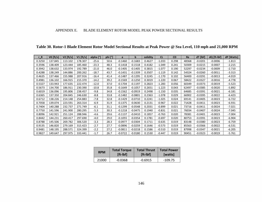
146

APPENDIX E. BLADE ELEMENT ROTOR MODEL PEAK POWER SECTIONAL RESULTS

Table 30. Rotor-1 Blade Element Rotor Model Sectional Results at Peak Power @ Sea Level, 110 mph and 21,000 RPM

r_R V0 [ft/s] V2 [ft/s] V1 [ft/s] alpha [°] phi [°] a b solidity CL CD Re dT [lbf] dQ [ft-lbf] dP [Watts]

0.3250 137.845 113.102 178.307 -25.6 50.6 -0.1460 -0.1683 0.4627 -1.033 0.298 48368 -0.0201 -0.0006 -1.813

0.3596 138.409 123.444 185.460 -23.3 48.3 -0.1418 -0.1518 0.4182 -1.049 0.241 50309 -0.0215 -0.0007 -2.215

0.3942 138.632 133.974 192.789 -21.0 46.0 -0.1405 -0.1405 0.3815 -1.077 0.190 52297 -0.0234 -0.0009 -2.710

0.4288 138.249 144.886 200.262 -18.7 43.7 -0.1431 -0.1339 0.3507 -1.119 0.142 54324 -0.0260 -0.0011 -3.313

0.4635 137.466 155.988 207.916 -16.4 41.4 -0.1487 -0.1295 0.3245 -1.170 0.102 56400 -0.0291 -0.0013 -4.019

0.4981 136.102 166.915 215.370 -14.2 39.2 -0.1569 -0.1250 0.3019 -1.220 0.067 58422 -0.0327 -0.0016 -4.778

0.5327 133.943 177.635 222.474 -12.0 37.0 -0.1704 -0.1197 0.2823 -1.283 0.056 60349 -0.0373 -0.0019 -5.523

0.5673 134.700 186.911 230.390 -10.8 35.8 -0.1649 -0.1057 0.2651 -1.223 0.043 62497 -0.0385 -0.0020 -5.892

0.6019 136.096 195.806 238.457 -9.8 34.8 -0.1562 -0.0919 0.2498 -1.150 0.035 64685 -0.0391 -0.0021 -6.181

0.6365 137.350 204.845 246.630 -8.8 33.8 -0.1482 -0.0801 0.2363 -1.078 0.029 66902 -0.0395 -0.0022 -6.423

0.6712 138.226 214.148 254.883 -7.8 32.8 -0.1429 -0.0710 0.2241 -1.025 0.024 69141 -0.0405 -0.0023 -6.722

0.7058 139.074 223.591 263.314 -6.9 31.9 -0.1375 -0.0630 0.2131 -0.967 0.022 71428 -0.0411 -0.0023 -6.931

0.7404 140.288 232.737 271.749 -6.1 31.1 -0.1299 -0.0548 0.2031 -0.899 0.021 73716 -0.0411 -0.0024 -7.021

0.7750 141.596 241.900 280.295 -5.3 30.3 -0.1218 -0.0475 0.1940 -0.831 0.021 76034 -0.0407 -0.0024 -7.045

0.8096 142.921 251.124 288.946 -4.6 29.6 -0.1137 -0.0410 0.1857 -0.763 0.020 78381 -0.0401 -0.0023 -7.004

0.8442 144.231 260.417 297.690 -4.0 29.0 -0.1055 -0.0354 0.1781 -0.697 0.020 80753 -0.0391 -0.0023 -6.904

0.8788 145.506 269.782 306.520 -3.3 28.3 -0.0977 -0.0304 0.1711 -0.635 0.019 83148 -0.0380 -0.0023 -6.759

0.9135 146.820 279.169 315.423 -2.7 27.7 -0.0896 -0.0259 0.1646 -0.573 0.019 85563 -0.0366 -0.0022 -6.531

0.9481 148.195 288.571 324.399 -2.2 27.2 -0.0811 -0.0218 0.1586 -0.510 0.019 87998 -0.0347 -0.0021 -6.205

0.9827 149.647 297.975 333.441 -1.7 26.7 -0.0722 -0.0180 0.1530 -0.447 0.019 90451 -0.0323 -0.0019 -5.761

RPM Total Torque

[ft-lbf] Total Thrust

[ft-lbf] Total Power

[watts]

21000 -0.0368 -0.6915 -109.75

147

Table 31. Rotor-2 Blade Element Rotor Model Sectional Results at Peak Power @ Sea Level, 110 mph and 21,000 RPM

r_R V0 [ft/s] V2 [ft/s] V1 [ft/s] alpha [°] phi [°] a b solidity CL CD Re dT [lbf] dQ [ft-lbf] dP [Watts]

0.3250 139.469 120.704 184.448 -9.8 49.1 -0.1356 -0.2466 0.4627 -1.146 0.035 50034 -0.0188 -0.0009 -2.685

0.3596 140.388 128.782 190.509 -9.3 47.5 -0.1299 -0.2020 0.4182 -1.113 0.032 51678 -0.0201 -0.0010 -2.998

0.3942 141.020 137.293 196.815 -8.9 45.8 -0.1259 -0.1689 0.3815 -1.081 0.029 53389 -0.0214 -0.0011 -3.315

0.4288 141.391 146.176 203.369 -8.4 44.0 -0.1236 -0.1441 0.3507 -1.056 0.026 55167 -0.0229 -0.0012 -3.650

0.4635 141.597 155.413 210.244 -8.0 42.3 -0.1223 -0.1251 0.3245 -1.031 0.024 57032 -0.0245 -0.0013 -3.990

0.4981 141.689 164.693 217.255 -7.6 40.7 -0.1218 -0.1095 0.3019 -1.011 0.023 58933 -0.0263 -0.0015 -4.340

0.5327 141.677 174.122 224.479 -7.3 39.1 -0.1219 -0.0970 0.2823 -0.992 0.022 60893 -0.0281 -0.0016 -4.702

0.5673 141.577 183.678 231.909 -7.0 37.6 -0.1225 -0.0867 0.2651 -0.975 0.022 62909 -0.0301 -0.0017 -5.075

0.6019 141.388 193.349 239.530 -6.8 36.2 -0.1237 -0.0782 0.2498 -0.961 0.022 64976 -0.0322 -0.0018 -5.463

0.6365 141.136 203.295 247.484 -6.6 34.8 -0.1255 -0.0716 0.2363 -0.948 0.022 67134 -0.0345 -0.0020 -5.870

0.6712 140.737 213.187 255.452 -6.6 33.4 -0.1280 -0.0658 0.2241 -0.941 0.021 69295 -0.0371 -0.0021 -6.309

0.7058 140.208 223.159 263.549 -6.5 32.1 -0.1313 -0.0611 0.2131 -0.938 0.021 71492 -0.0399 -0.0023 -6.781

0.7404 139.550 233.214 271.778 -6.5 30.9 -0.1355 -0.0571 0.2031 -0.938 0.021 73724 -0.0430 -0.0024 -7.290

0.7750 138.760 243.345 280.127 -6.6 29.7 -0.1404 -0.0538 0.1940 -0.942 0.021 75988 -0.0464 -0.0026 -7.840

0.8096 137.837 253.539 288.585 -6.7 28.5 -0.1462 -0.0511 0.1857 -0.949 0.022 78283 -0.0501 -0.0028 -8.431

0.8442 136.785 263.786 297.142 -6.8 27.4 -0.1528 -0.0488 0.1781 -0.959 0.022 80604 -0.0542 -0.0030 -9.062

0.8788 135.613 274.072 305.788 -7.0 26.3 -0.1602 -0.0468 0.1711 -0.972 0.022 82949 -0.0587 -0.0033 -9.730

0.9135 134.332 284.383 314.514 -7.2 25.3 -0.1683 -0.0450 0.1646 -0.986 0.022 85316 -0.0635 -0.0035 -10.427

0.9481 132.774 294.614 323.151 -7.4 24.3 -0.1775 -0.0433 0.1586 -0.999 0.023 87659 -0.0685 -0.0037 -11.111

0.9827 131.246 304.950 331.994 -7.7 23.3 -0.1870 -0.0419 0.1530 -1.015 0.023 90058 -0.0740 -0.0040 -11.839

RPM Total Torque

[ft-lbf] Total Thrust

[ft-lbf] Total Power

[watts]

21000 -0.0439 -0.7944 -130.91

EVALUATION OF DESIGN TOOLS FOR THE MICRO-RAM AIR …

Documents

Transcript of EVALUATION OF DESIGN TOOLS FOR THE MICRO-RAM AIR …