Evaluation of Design Loads for Concrete Bridge Rails

Evaluation of Design Loads for Concrete Bridge Rails

Contract # DTRT12GUTC12 with USDOT Office of the Assistant Secretary for Research and Technology (OST-R)

Final Report

March 2016

Principal Investigator: Dr. Dean Sicking, University of Alabama at Birmingham National Center for Transportation Systems Productivity and Management O. Lamar Allen Sustainable Education Building 788 Atlantic Drive, Atlanta, GA 30332-0355 P: 404-894-2236 F: 404-894-2278 [email protected] nctspm.gatech.edu

DISCLAIMER

The contents of this report reflect the views of the authors, who are responsible for the facts and the

accuracy of the information presented herein. This document is disseminated under the sponsorship of

the U.S. Department of Transportation’s University Transportation Centers Program, in the interest of

information exchange. The U.S. Government assumes no liability for the contents or use thereof.

UAB SCHOOL OF ENGINEERING

Evaluation of Design Loads for Concrete Bridge Rails

By

Kevin Schrum, Ph.D.

Instructor, Research Engineer University of Alabama at Birmingham

School of Engineering 371A Hoehn Engineering Building

1075 13th Street South (205) 934-8470

[email protected]

Dean Sicking, Ph.D., P.E. Professor, Associate VP for Product Development

University of Alabama at Birmingham School of Engineering

371B Hoehn Engineering Building 1075 13th Street South

(205) 934-8492 [email protected]

Nasim Uddin, PhD, P.E., F.ASCE

Professor University of Alabama at Birmingham

School of Engineering 321 Hoehn Engineering Building

1075 13th Street South (205) 934-8432

[email protected]

3/1/2016

DISCLAIMER

This report was completed with funding from the Alabama Department of Transportation

(DOT). The contents of this report reflect the view and opinions of the authors who are

responsible for the facts and the accuracy of the data presented herein. The contents do not

necessarily reflect the official views or policies of the Alabama DOT or any other governing

body. This report does not constitute a standard, specification, or regulation.

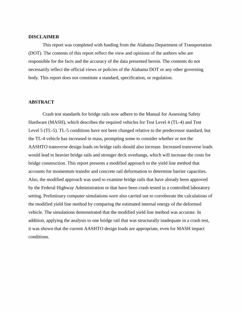
ABSTRACT

Crash test standards for bridge rails now adhere to the Manual for Assessing Safety

Hardware (MASH), which describes the required vehicles for Test Level 4 (TL-4) and Test

Level 5 (TL-5). TL-5 conditions have not been changed relative to the predecessor standard, but

the TL-4 vehicle has increased in mass, prompting some to consider whether or not the

AASHTO transverse design loads on bridge rails should also increase. Increased transverse loads

would lead to heavier bridge rails and stronger deck overhangs, which will increase the costs for

bridge construction. This report presents a modified approach to the yield line method that

accounts for momentum transfer and concrete rail deformation to determine barrier capacities.

Also, the modified approach was used to examine bridge rails that have already been approved

by the Federal Highway Administration or that have been crash tested in a controlled laboratory

setting. Preliminary computer simulations were also carried out to corroborate the calculations of

the modified yield line method by comparing the estimated internal energy of the deformed

vehicle. The simulations demonstrated that the modified yield line method was accurate. In

addition, applying the analysis to one bridge rail that was structurally inadequate in a crash test,

it was shown that the current AASHTO design loads are appropriate, even for MASH impact

conditions.

Table of Contents 1. Introduction ............................................................................................................... 1

Background ........................................................................................................... 1

Problem Statement ................................................................................................ 6

Objectives .............................................................................................................. 6

Scope ..................................................................................................................... 7

2. Research Approach ................................................................................................... 8

Develop a Modified YLM ..................................................................................... 8

Analyze Existing Concrete Bridge Rails ............................................................... 9

Energy Verification with LS-DYNA .................................................................. 10

3. Modified Yield Line Method .................................................................................. 11

Mechanics............................................................................................................ 11

3.1.1. Impact Severity ............................................................................................. 11

3.1.3. Conservation of Linear Momentum .............................................................. 13

3.1.4. Conservation of Energy ................................................................................ 14

3.1.5. Governing Equation ...................................................................................... 15

Moment Capacities .............................................................................................. 15

4. Analysis of Existing Concrete Bridge Rails ........................................................... 18

Selected Barriers and Moment Capacities .......................................................... 18

Iterative Solution for Effective Length ............................................................... 19

Barrier Capacities Based on Modified YLM ...................................................... 21

5. Energy Verification via LS-DYNA ........................................................................ 24

Introduction ......................................................................................................... 24

Concrete Beam Testing ....................................................................................... 25

Material Model .................................................................................................... 27

Internal Energy of Truck ..................................................................................... 30

6. Discussion of Results .............................................................................................. 33

7. Conclusions and Recommendations ....................................................................... 35

8. References ............................................................................................................... 37

9. Appendices .............................................................................................................. 38

A. Barrier Moment Capacity Calculations ............................................................... 39

1. Vertical Wall .................................................................................................... 40

2. Single Slope ..................................................................................................... 41

3. F-Shape ............................................................................................................ 43

4. New Jersey Shape – 32” .................................................................................. 45

5. New Jersey Shape – 36” .................................................................................. 47

6. New Jersey Shape – 42” .................................................................................. 49

7. New Jersey Shape – 54” .................................................................................. 52

Table of Figures

Figure 1. Mathematical Model of Vehicle - Barrier Railing Collision [6] ......................... 2

Figure 2. List of Variable Definitions Used by Hirsch [1] ................................................. 3

Figure 3. Distribution of Impact Load in Collision with Longitudinal Traffic Rail [1]. .... 4

Figure 4. Yield Line Analysis of Concrete Parapet Wall [1]. ............................................. 4

Figure 5. Schematic of Barrier Displacement. .................................................................. 12

Figure 6. Iterative Problem Setup ..................................................................................... 20

Figure 7. Goal Seek Selection ........................................................................................... 20

Figure 8. Goal Seek Programming.................................................................................... 21

Figure 9. Goal Seek Results .............................................................................................. 21

Figure 10. Beam Test Setup with Speed Dowels and Track Guidance ............................ 26

Figure 11. Bogey Impact Head and Orientation ............................................................... 26

Figure 12. Steel Rebar Material Card ............................................................................... 28

Figure 13. Concrete Material Card ................................................................................... 29

Figure 14. Design 3 Comparisons ..................................................................................... 29

Figure 15. Impact Orientation of Bridge Rail Impact ....................................................... 31

Figure 16. TL-4 Test Vehicle Dimensional Drawing ....................................................... 34

Table of Tables

Table 1. Moment Capacities of Analyzed Barriers ........................................................... 19

Table 2. Summary of Barrier Capacities ........................................................................... 22

Table 3. Summary of Truck Internal Energy .................................................................... 23

Table 4. Expected Moment Capacities for Beam Designs ............................................... 27

1

1. INTRODUCTION

Background

In the mid to late 1970s, T.J. Hirsch developed what is now called the Yield Line Method

(YLM) to analyze the crash test results of some Texas bridge rails that were impacted with buses

and trucks [1]. The bridge deck was not included in the analysis. The bridge rail itself was

treated as a rigid object that was defined by sections that were separated by yield lines. Often, a

vertical crack formed at the point of contact, and two angled cracks extended from the bottom of

the vertical crack in the upstream and downstream directions. The YLM attempts to estimate the

bridge rails capacity assuming that these yield lines represent a state of failure. To do so, three

moment capacities must be defined: (1) beam; (2) wall; and (3) cantilever. For bridge rails with a

discernible beam at the top, this first moment capacity would be non-zero, but for a majority of

safety shapes, this beam moment capacity is assumed to be zero. The wall moment capacity is

defined by both the Whitney stress block of the concrete and the reinforcement design through

the cross-section of the bridge rail. The cantilever moment capacity is determined from the

stirrup/overhang interface reinforcement, including the spacing the rebar longitudinally as well

as the concrete strength and width at the interface between the rail and the deck.

Hirsch analyzed crash test data to determine forces acting on the wall from the vehicle.

He then compared his analytic prediction with the data, and when the YLM overpredicted the

barrier capacity, Hirsch used engineering judgment to reduce the predicted force from the YLM.

With these adjusted results, he recommended the design loads that the American Association of

State Highway Transportation Officials (AASHTO) requires in their bridge design specification

[37]. The most recent publication recommends transverse design loads of 54 kips and 124 kips

for Test Level (TL) 4 and TL-5, respectively. These specifications were believed to apply

adequately to the National Cooperative Highway Research Program (NCHRP) Report No. 350

(NCHRP 350) test conditions, which were set forth in 1993 [37]. TL-4 was defined by an impact

with an 18,000-lb single-unit truck, whereas TL-5 was defined by an impact with an 80,000-lb

semi-tractor trailer.

Hirsch reviewed the equations presented in NCHRP Report 86 [6], as described in

Equations 1 through 4. The parameters for these equations can be found in Hirsch’s report, and

are repeated in Figure 1 and Figure 2. These equations were used to analyze crash test data.

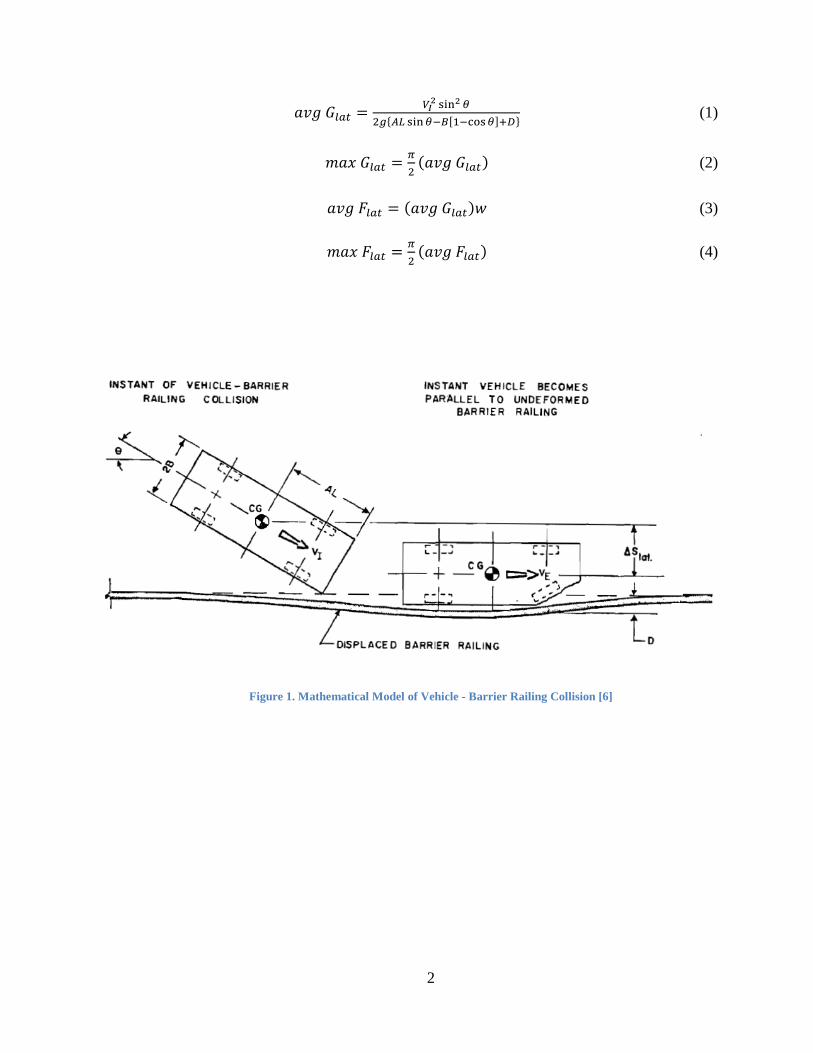
2

𝑎𝑎𝑎𝑎𝑎𝑎 𝐺𝐺𝑙𝑙𝑙𝑙𝑙𝑙 = 𝑉𝑉𝐼𝐼2 sin2 𝜃𝜃

2𝑔𝑔{𝐴𝐴𝐿𝐿 sin𝜃𝜃−𝐵𝐵[1−cos𝜃𝜃]+𝐷𝐷} (1)

𝑚𝑚𝑎𝑎𝑚𝑚 𝐺𝐺𝑙𝑙𝑙𝑙𝑙𝑙 = 𝜋𝜋2

(𝑎𝑎𝑎𝑎𝑎𝑎 𝐺𝐺𝑙𝑙𝑙𝑙𝑙𝑙) (2)

𝑎𝑎𝑎𝑎𝑎𝑎 𝐹𝐹𝑙𝑙𝑙𝑙𝑙𝑙 = (𝑎𝑎𝑎𝑎𝑎𝑎 𝐺𝐺𝑙𝑙𝑙𝑙𝑙𝑙)𝑤𝑤 (3)

𝑚𝑚𝑎𝑎𝑚𝑚 𝐹𝐹𝑙𝑙𝑙𝑙𝑙𝑙 = 𝜋𝜋2

(𝑎𝑎𝑎𝑎𝑎𝑎 𝐹𝐹𝑙𝑙𝑙𝑙𝑙𝑙) (4)

Figure 1. Mathematical Model of Vehicle - Barrier Railing Collision [6]

3

Figure 2. List of Variable Definitions Used by Hirsch [1]

Then, Hirsch developed the yield line method to predict the strength of a bridge rail based

solely on the design of the barrier. Regardless of the barrier type, the impact conditions were

illustrated in a similar manner, as seen in Figure 3. For concrete bridge rails, the key components

of the analysis were labeled as shown in Figure 4.

4

Figure 3. Distribution of Impact Load in Collision with Longitudinal Traffic Rail [1].

Figure 4. Yield Line Analysis of Concrete Parapet Wall [1].

With these definitions, Hirsch developed his yield line equations to determine the load on

the barrier that induced yielding (𝑤𝑤𝑤𝑤) and the length of the yielded portion (𝐿𝐿), according to

Equations 5 and 6, respectively.

5

𝑤𝑤𝑤𝑤 = 8𝑀𝑀𝑏𝑏𝐿𝐿∙𝑙𝑙 2�

+ 8𝑀𝑀𝑤𝑤𝐻𝐻𝐿𝐿−𝑙𝑙 2�

+ 𝑀𝑀𝑐𝑐𝐿𝐿2

𝐻𝐻�𝐿𝐿−𝑙𝑙 2� � (5)

𝐿𝐿 = 𝑙𝑙2

+ ��𝑙𝑙2�2

+ 8𝐻𝐻(𝑀𝑀𝑏𝑏+𝑀𝑀𝑤𝑤𝐻𝐻)𝑀𝑀𝑐𝑐

(6)

Where:

𝑤𝑤𝑤𝑤 = total ultimate load capacity of the wall, kips

𝑤𝑤 = length of distributed impact load, ft

𝑀𝑀𝑏𝑏 = ultimate moment capacity of a beam at the top of the wall, kip-ft

𝑀𝑀𝑤𝑤 = ultimate moment capacity of the wall per foot of wall height, kip-ft/ft

𝑀𝑀𝑐𝑐 = ultimate moment capacity of the wall cantilever up from the bridge deck per foot of

length of wall, kip-ft/ft

𝐻𝐻 = height of wall, ft

𝐿𝐿 = critical length of wall failure, ft

Hirsch’s work focused on buses and heavy vehicles. Buses fall between test levels of the

previous and current crash test standard, in terms of impact severity. The design loads

recommended by Hirsch were adopted even after NCHRP 350 test conditions were established in

1993 and remained in effect until 2009.

Since 2009, the Manual for Assessing Safety Hardware (MASH) [37] has replaced

NCHRP 350, an in many cases, the impact energy was increased to match the modern vehicle

fleet. The TL-4 vehicle increased to approximately 22,000 lbs, but the TL-5 vehicle was

unchanged. Intuitively, with a larger vehicle, it may be expected that the design load would

increase from the NCHRP 350 levels. However, the designs generated from the previous test

standard impact conditions have not led to a nationwide pandemic of failing bridge rails.

Vehicles have gotten larger, but the bridge rail designs have essentially remained unchanged,

with the exception of barrier height. This increase in height was intended to address rollover in

taller vehicles, not an increase in transverse load. Despite this observation, some researchers

have conducted analyses via the finite element method (computer simulation) to determine what

loads are being imparted on bridge rails. Their recommendations were to increase the TL-4

6

design load to 80 kips and the TL-5 load to at least 160 kips (for barriers shorter than 42 inches)

and up to 260 kips (for barriers taller than 42 inches) [37].

Problem Statement

By increasing required design loads, new bridge rails will be wider and carry more steel,

making them heavier and more costly. The cost considerations are further compounded when the

additional dead load is considered in the design of the overhang deck. Before such magnanimous

policy changes are instituted, which could substantially hamper any State highway budget, these

design loads need to be examined further.

Particularly, there does not seem to be a large contingency of cases where the bridge rail

was insufficient capacity when struck by a large vehicle. That hypothetical bridge rail was most

likely designed according to the specifications currently in AASHTO. It is worth noting that the

AASHTO design loads were based on some engineering judgment and for vehicle classes that do

not directly correspond with NCHRP 350 or MASH test vehicles. As such, it may be possible

that the current design loads were already conservative. There hasn’t been an illustrated need to

increase these design loads yet. However, MASH has only been in place since 2009. Therefore,

the possibility exists that the new expected loads, from the larger vehicles, may necessitate an

increase in design loads.

In addition to engineering judgment, Hirsch, and almost everyone that has followed after

him, made assumptions of rigidity in the barrier and deck. The barrier may be loaded through a

large deformed area, especially for the longer semi-tractor trailer vehicles. With the wide variety

of barrier shapes and heights, the energy absorption inherent in the bending and rotating of the

barrier need to be considered. Also, the current YLM ignores the crush of the vehicle as a source

of energy dissipation. Before extremely expensive design policies are implement, each of these

components must be analyzed.

Objectives

This research project was intended to determine appropriate concrete bridge rail design

loads such that MASH-style vehicles could not cause any structural damage to the rail. To do so,

the YLM method was modified to account for momentum transfer between the vehicle and the

barrier as well as internal energy due to crush of the vehicle. Finally, with the analysis complete,

7

this research effort will identify a minimum safety performance for which a crash test occurred

and no structural damage was taken by the barrier. Finally, this minimum will be compared to

existing capacity requirements and TTIs recommended specifications and will recommend the

appropriate design loads that should be adopted as minimum transverse design loads for TL-4

and TL-5 only.

Scope

The proposed recommendations for design loads applies to concrete bridge rails only. It

is intended to evaluate the design specifications only, but the methodology may be adapted for

new designs, so long as any new bridge rail is thoroughly evaluated and crash tested according to

the most recent crash test standard. This research does not apply to post-and-beam style bridge

rails because it requires a relatively constant cross-sectional area for mass calculations.

8

2. RESEARCH APPROACH

Develop a Modified YLM

Hirsch’s original formulation of the YLM to evaluate the capacity of bridge rails assumed

rigidity in the bridge rail. It also did not account for the crush of the vehicle as a substantial

source of energy dissipation. Therefore, the first step in this project was to develop a modified

YLM that incorporated barrier deformation and vehicle crush in the analysis.

In the traditional YLM, a critical length of barrier must be determined. Originally, this

length was a function of the three moment capacities and the height of the barrier, in addition to

the width of the distributed load. Fundamentally, the modified YLM proposed herein relies on

many of the same calculations as the traditional YLM, but the primary difference is the way in

which the critical length is calculated. This new approach will use linear momentum and internal

energy to establish the critical length.

The law of conservation of linear momentum for a perfectly plastic impact between two

objects states that the velocity of the two-object system will be equal to the sum of the

momentums of the two objects prior to impact divided by the combined mass of the two objects.

In this case, the bridge is stationary (initial velocity and momentum are zero), and the new

velocity becomes the initial velocity of the truck times the ratio of the truck’s mass to the

combined mass. The critical length determines the mass of the barrier, since mobilizing the entire

bridge rail is generally not possible. In other words, only a portion of the bridge rail moves upon

impact with the vehicle. The critical length defines this portion.

Strain energy in the barrier and internal energy in the vehicle are both derived from the

law of conservation of linear momentum. The barrier is accelerated, and therefore deformed, thus

absorbing energy. The amount of this deformation is dependent on the load, but boundary

conditions can be applied to ascertain a specific performance. In this case, the maximum strain in

the rebar was not to exceed 6%. Using a simplified deformation shape of the barrier, this strain

limit was used to calculate the deformed area of the concrete, which was then used to calculate

the strain energy in the barrier.

Next, the reduced velocity of the truck following the inertial momentum transfer was

used to calculate a new kinetic energy using the velocity component that was perpendicular to

9

the barrier. The difference in this new energy and the original impact energy constitutes the

change in internal energy of the truck due to crush.

Finally, the Impact Severity (IS) of the truck prior to impact was set equal to the sum of

the barrier’s strain energy and the vehicles change in internal energy. This equation yields one

unknown parameter, the critical length. However, it is a non-linear equation and required

iterative numerical methods to calculate the critical length. The resistive capacity of the barrier

was then determined as a function of this critical length and other parameters in a simple, linear

equation.

Analyze Existing Concrete Bridge Rails

After the modified YLM was mathematically derived, it was applied to numerous

existing concrete bridge rails. The concept was that if the barrier had been crash tested, then the

test agency would have noted any structural damage to the barrier as a result of the loads

imparted from the vehicle to the bridge rail. After determining the barrier’s capacity from the

modified YLM, the crash test reports for the weakest barriers were reviewed to determine their

structural performance in the crash test.

First, all bridge rails considered crashworthy by the Federal Highway Administration

(FHWA) were identified, and any associated cross-sectional drawings provided either by the

FHWA or by another entity (such as TTI or the New Jersey Turnpike Authority) were gathered.

From these drawings, the cross-sectional area was calculated, which is a crucial component in

the modified YLM.

The drawings also contained the reinforcement design and details on the compressive

strength of the concrete. From these parameters, the moment capacities for each bridge rail were

calculated. Generally, the beam moment capacity was zero, so long as no additional beam

elements were included at the top of the rail. The wall and cantilever capacities were functions of

the longitudinal and shear reinforcement, respectively.

Next, the moment capacities and barrier height were plugged into the modified YLM

governing equation, and by the process of iteration, the critical length was calculated. Once this

10

length was determined, a simple equation was used to determine the resistive capacity of the

barrier. These two calculations were dependent on the loading conditions (i.e., TL-4 or TL-5).

Energy Verification with LS-DYNA

The governing equation of the modified YLM contained three components: (1) impact

severity; (2) strain energy of the barrier; and (3) the change in internal energy of the truck. All

three of these components are linked to one another. The IS is a constant and must be absorbed

by the other two components. Hypothetically, if the strain energy of the barrier decreases, then

the vehicle’s change in internal energy would have to increase.

The balance of this governing equation was investigated by examining the total change in

internal energy of truck using LS-DYNA, a non-linear explicit finite element analysis code

developed by Livermore Software Technology Cooperation (LSTC). A single unit truck model

was publicly available through the archive of the National Crash Analysis Center (NCAC). The

bridge rail geometry matched a standard 32-inch New Jersey safety shape bridge rail, which was

simulated with a built-in concrete model, *MAT_159. This material model provides the freedom

to adjust the compressive strength, average aggregate size, and damage coefficient. This final

term was calibrated by comparing a model to physical testing of reinforced concrete beams.

These beams were impacted by a bogey vehicle at the Barber Laboratory for Advanced Safety

Education and Research (BLASER) in Leeds, AL. With a calibrated concrete material model, the

research team could confidently assume that the strain energy in the barrier was accurate. LS-

DYNA does not currently provide post-processing for strain energy. Therefore, the internal

energy of the vehicle was studied to corroborate the governing equation of the modified YLM.

11

3. MODIFIED YIELD LINE METHOD

The YLM was modified to determine the critical length of the barrier in a more inclusive

way. In particular, the strain energy developed due to the barrier’s deflection and the change in

internal energy of the vehicle due to its crush were incorporated. The governing principle of the

modified yield line method is displayed as Equation 7:

(𝐼𝐼𝐼𝐼) = (𝐼𝐼𝑆𝑆 𝑖𝑖𝑖𝑖 𝐵𝐵𝑎𝑎𝐵𝐵𝐵𝐵𝑖𝑖𝐵𝐵𝐵𝐵) + (∆𝐼𝐼𝑆𝑆 𝑜𝑜𝑜𝑜 𝑡𝑡ℎ𝐵𝐵 𝑉𝑉𝐵𝐵ℎ𝑖𝑖𝑖𝑖𝑤𝑤𝐵𝐵) (7)

Where:

𝐼𝐼𝐼𝐼 = Impact Severity, kip-ft

𝐼𝐼𝑆𝑆 = Strain Energy, kip-ft

∆𝐼𝐼𝑆𝑆 = Change in Internal Energy, kip-ft

To understand and assemble the components of Equation 7, a cursory discussion on

impact severity, strain energy, momentum, and energy were presented in the sections that follow.

Following the description of these elements, Equation 7 will be fully assembled, and the

procedure for calculating the new critical length will be provided.

Mechanics

3.1.1. Impact Severity

The impact condition shown in Figure 1 includes a mass, velocity, and impact angle for

the vehicle. By definition, velocity is a vector, which means it is a speed with a direction. That

speed, combined with the vehicle’s mass, can be used to calculate the kinetic energy of the

vehicle. However, the barrier only resists the perpendicular component of that velocity.

Therefore, the energy dissipation required to arrest the vehicle’s perpendicular velocity, or

become parallel with the barrier, is given by the Impact Severity (IS). Note the constant (1/1000)

converts the IS from lb-ft to kip-ft.

𝐼𝐼𝐼𝐼 = 12𝑚𝑚(𝑎𝑎 sin𝜃𝜃)2 ∙ 1

1000 (8)

Where:

𝑚𝑚 = Mass of the vehicle, lb-ft/s2 (slugs) = 𝑊𝑊𝑇𝑇 𝑎𝑎⁄

12

𝑊𝑊𝑇𝑇 = Weight of the vehicle, lbs

𝑎𝑎 = Acceleration due to gravity, 32.174 ft/s2

𝑎𝑎 = Velocity of the vehicle, ft/s

𝜃𝜃 = Impact angle, degrees

3.1.2. Strain Energy

In its most basic form, strain energy is the energy stored by a deformed object. For this

project, the strain energy was defined as the external force times the displaced distance of the

barrier. This external force was the maximum force the barrier could withstand based on its three

moment capacities and its height. The displacement was determined from the maximum strain in

the rebar, assuming a maximum of 6% strain. This limit corresponds closely with the onset of

strain hardening in tensile tests conducted on steel rebar and also on a required minimum strain

at fracture for rebar [7]. The determination of the displacement in the barrier was based on the

schematic shown in Figure 5.

Figure 5. Schematic of Barrier Displacement.

Engineering strain is defined as the change in length divided by the original length. It

represents a stretch. If the strain is prescribe, such as 6% in this case, then the new length, L’,

drops out of the equation when determining the displacement, ∆. Starting with the mathematical

definition of strain in Equation 9, the derivation for the displacement follows in Equations 9

through 12.

ε = 𝐿𝐿′−𝐿𝐿𝐿𝐿

= 0.06 (9)

𝐿𝐿′ = 1.06 ∙ 𝐿𝐿 (10)

13

∆= ��𝐿𝐿′2�2

+ �𝐿𝐿2�2 (11)

Substituting Equation 10 into Equation 11, the displacement reduces to:

∆= 𝐿𝐿√0.0309 (12)

For now, this definition will suffice until all the components of Equation 7 are defined.

The displacement is a function of the effective length of the barrier, which is unknown.

However, to finish the strain energy component, Equation 12 must be multiplied by the barriers

strength. This strength was a function of the barrier’s height, reinforcement, and effective length,

again. Hirsch’s equation for barrier capacity was substituted into the analysis at this juncture.

The force require to induce 6% strain in the rebar was given by Equation 13.

𝐹𝐹 = 8𝑀𝑀𝑏𝑏𝐿𝐿

+ 8𝑀𝑀𝑤𝑤𝐻𝐻𝐿𝐿

+ 𝑀𝑀𝑐𝑐𝐿𝐿𝐻𝐻

(13)

Where:

𝐹𝐹 = Force required to induce 6% strain in the barrier, kips

𝐿𝐿 = Effective length of the barrier, ft

All other terms are as defined earlier. Combining Equations 12 and 13, the strain energy

in the barrier for 6% strain in the rebar is given in Equation 14:

𝐼𝐼𝑆𝑆 = 𝐿𝐿√0.0309 �8𝑀𝑀𝑏𝑏𝐿𝐿


+ 𝑀𝑀𝑐𝑐𝐿𝐿𝐻𝐻� (14)

3.1.3. Conservation of Linear Momentum

When two objects collide in a perfectly plastic manner, they move together with the same

velocity. If one of those objects is stationary, it must be accelerated; whereas, the other object

must be decelerated. The resulting velocity of the two-object system is equivalent to the impact

velocity of the moving object times the ratio of the mass of the moving object and the total mass

of the two-object system. This definition of velocity is defined in Equation 15. The two objects

were a vehicle and a portion of the barrier. The length of this portion determines the mass that

needs to be accelerated. Incidentally, it is also the effective length discussed in the previous

section and it replaces the critical length from Hirsch’s original YLM.

14

𝑎𝑎𝑓𝑓 = 𝑚𝑚1𝑚𝑚1+𝑚𝑚2

∙ 𝑎𝑎𝑖𝑖 (15)

Where:

𝑎𝑎𝑓𝑓 = Final velocity of the two-object system, ft/s

𝑎𝑎𝑖𝑖 = Initial velocity of the vehicle, ft/s

𝑚𝑚1 = Mass of the vehicle, lb-ft/s2 (slugs) = 𝑊𝑊𝑇𝑇/𝑎𝑎

𝑚𝑚2 = Effective mass of the barrier, lb-ft/s2 (slugs) = 𝜌𝜌 ∙ 𝐴𝐴 ∙ 𝐿𝐿

𝜌𝜌 = Density of the concrete barrier = 150 lb/ft3

𝐴𝐴 = Cross-sectional area of the concrete barrier, ft2

Here, again, the effective length, 𝐿𝐿, was required. Substituting the mass terms for

weights, Equation 15 can be rewritten as Equation 16. Note that the constant of gravity drops out

of the equation.

𝑎𝑎𝑓𝑓 = 𝑊𝑊𝑇𝑇𝑊𝑊𝑇𝑇+150∙𝐴𝐴∙𝐿𝐿

∙ 𝑎𝑎𝑖𝑖 (16)

3.1.4. Conservation of Energy

While accelerating the barrier, the impact zone on the vehicle will crush. This crush is

mostly characterized by large-scale plastic deformation and fracture of the steel and plastic in

and around the impact zone. All of this damage absorbs energy. The summation of this energy

absorption was call the change in internal energy of the vehicle. It was equal to the difference in

kinetic energy of the vehicle following the transfer of momentum, as discussed in the previous

section. First, the initial and final kinetic energies, by definition, are given in Equations 17 and

18, respectively.

𝐾𝐾𝑆𝑆𝑖𝑖 = 𝑊𝑊𝑇𝑇2𝑔𝑔∙ 𝑎𝑎𝑖𝑖2 (17)

𝐾𝐾𝑆𝑆𝑓𝑓 = 𝑊𝑊𝑇𝑇2𝑔𝑔∙ 𝑎𝑎𝑓𝑓2 (18)

Where:

𝐾𝐾𝑆𝑆𝑖𝑖 = Initial kinetic energy of the vehicle, kip-ft

𝐾𝐾𝑆𝑆𝑓𝑓 = Final kinetic energy of the vehicle, kip-ft

15

The difference in the initial and final kinetic energy is theoretically equal to the change in

the internal energy of the truck. Taking this difference and substituting Equation 16 into

Equation 18 results in Equation 19. Note the constant (1/1000) at the end of the equation

converts the units from lb-ft to kip-ft.

∆𝐼𝐼𝑆𝑆 = 𝑊𝑊𝑇𝑇2𝑔𝑔∙ 𝑎𝑎𝑖𝑖2 ∙ �1 −

𝑊𝑊𝑇𝑇𝑊𝑊𝑇𝑇+150∗𝐴𝐴∗𝐿𝐿

� ∙ 11000

(19)

3.1.5. Governing Equation

Equation 7 can now be completely assembled. Substituting Equations 8, 14, and 19 into

Equation 7 results in Equation 20. For the sake of conciseness, the unit conversion was applied to

the strain energy term, placing all three components in units of lb-ft.

𝑊𝑊𝑇𝑇2𝑔𝑔

(𝑎𝑎 𝑠𝑠𝑖𝑖𝑖𝑖 𝜃𝜃)2 = 1000 ∙ 𝐿𝐿√0.0309 �8𝑀𝑀𝑏𝑏𝐿𝐿


+ 𝑀𝑀𝑐𝑐𝐿𝐿𝐻𝐻� + 𝑊𝑊𝑇𝑇

2𝑔𝑔𝑎𝑎𝑖𝑖2 �1 −

𝑊𝑊𝑇𝑇𝑊𝑊𝑇𝑇+150∗𝐴𝐴∗𝐿𝐿

� (20)

Moment Capacities

A critical set of parameters in Equation 20 are the various moment capacities of the

barrier. The three moment capacities are: (1) beam, 𝑀𝑀𝑏𝑏; (2) wall, 𝑀𝑀𝑤𝑤; and (3) cantilever, 𝑀𝑀𝑐𝑐. All

three were illustrated in Hirsch’s diagram, which was reproduced in Figure 4. All three are

dependent on the reinforcement size and placement as well as the 28-day compressive strength of

the concrete and its cross-sectional dimensions. The yield strength of the rebar and the

compressive strength of the concrete were ascertained from the test reports or drawings of bridge

rails that are federally accepted for use on the National Highway System. Generally, the rebar

was comprised of Grade 60 steel, and the concrete had a compressive strength of between 3.6

and 4.0 ksi. Also, the portion of the concrete place in compressive due to external loading was

simplified by the Whitney stress block, which assumes that the compressive block is rectangular

in shape. The depth of this block was determined by Equation 21.

𝑎𝑎 = 𝐴𝐴𝑠𝑠𝑓𝑓𝑦𝑦𝛽𝛽1∙𝑓𝑓𝑐𝑐′∙𝑏𝑏

(21)

Where:

𝑎𝑎 = Height of the Whitney stress block, inches

𝐴𝐴𝑠𝑠 = Combined area of tensile steel rebar, in2

16

𝑜𝑜𝑦𝑦 = Yield stress of the rebar, ksi

𝛽𝛽1 = Reduction factor between 0.65 and 0.85

𝑜𝑜𝑐𝑐′ = 28-day compressive strength of concrete, ksi

𝑏𝑏 = width of the cross section, inches

This stress block defines the compressive side of the concrete, whereas the steel rebar in

tension defines the tensile side of the concrete. The two must be equilibrium. Using the distance

between the compressive forces (characterized by the midpoint of the stress block), the moment

capacity of the beam/wall/cantilever is that distance times the tensile capacity of the rebar.

Generally, the nominal moment capacity of a reinforced concrete design is given by Equation 22.

𝑀𝑀𝑁𝑁 = 𝐴𝐴𝑠𝑠𝑜𝑜𝑦𝑦 �𝑑𝑑 −𝑙𝑙2� (22)

Where:

𝑀𝑀𝑛𝑛 = Nominal moment capacity, kip-inch

𝑑𝑑 = Distance from the compressive face to the center of tensile reinforcement, inches

Most beam capacities were set to zero unless a distinguishable beam was observed on top

of the wall. The depth, 𝑑𝑑, was generally constant, with a symmetrical design. The flexion of the

beam, and the barrier in general, resulted in tension on both sides of the barrier at various stages.

At the location of peak displacement, for example, the backside of the barrier was in tension.

Because the location of the tensile stress could be on either side, the moment capacity for both

faces had to be determined. As aforementioned, for beams, these two values were generally

equal or zero.

For the wall capacity, 𝑀𝑀𝑤𝑤, the effective depth to the tensile steel was often dependent on

the vertical location of the rebar. For safety shapes, such as the New Jersey barrier, the impact

side of the bridge rail was sloped, resulting in decreasing depths as the height increased. To

calculate the wall capacity of these sloped shapes, individual calculations were carried out for

each level of rebar, which corresponded to a unique depth, 𝑑𝑑. Each individual level included the

area of one rebar, rather than all of the tensile rebar combined. Once the moment capacity for

each level was determined, they were all summed to provide the overall wall moment capacity.

This process was carried out for both faces, recognizing the possibility that the effective depths

17

could be different from some of the longitudinal rebars, especially those in the base portion of

the safety shape. For vertical walls or single slopes, this process only needed to be done once

since the moment capacities for both faces would be equal if the rebar was equidistant from both

faces. Finally, the resulting moment capacity was divided by the wall’s height, providing a

moment capacity per foot, or units of kip-ft/ft.

The cantilever moment capacity was determined by the interface steel design between the

deck overhang and the barrier. Generally, the shear reinforcement, or stirrups, of the barrier

extended down into the deck. The effective distance from the compressive side to the tensile

steel, a process that was repeated for both faces, was used to calculate the moment capacity. The

nominal moment capacity from this calculation was divided by the stirrup spacing to provide a

moment capacity per foot of wall, or units of kip-ft/ft.

18

4. ANALYSIS OF EXISTING CONCRETE BRIDGE RAILS

Selected Barriers and Moment Capacities

In order to install a concrete barrier anywhere on the National Highway System, it must

first be approved by the FHWA. Longitudinal barriers require crash testing with various vehicles

to ensure proper vehicle redirection and structural adequacy of the barrier. The FHWA maintains

a listing of acceptable concrete bridge rails on their website [8]. The heights and rebar design

may vary for each, but the general list of bridge rails studied in this report are as follows:

• Vertical Wall

• Single Slope

• F-Shape

• New Jersey Shape

In addition, bridge rails evaluated by Hirsch and crash tested by Bloom and Buth were

analyzed with the modified YLM. These barriers included the following [1]:

• T5

• T201

• T202

The hand calculations for each of these barriers are provided in Appendix A. For each set

of calculations, the tension face was considered to be on both sides because of the inflection

points in the rail displacement. Therefore, calculations were carried out for both sides,

distinguishing variations is rebar depth when necessary. Also, a 54-inch New Jersey barrier was

designed to provide a minimal level of performance as part of this project. It has not been crash

tested. The design itself is not recommended for use at this point. It would require full-scale

crash testing and FHWA approval before it could be implemented. The resulting moment

capacities for each of the barriers are listed in Table 1.

The T5 barrier was a particularly interesting case study. It was crash tested with a

40,000-lb intercity bus in 1976 [1]. The impact severity of this crash test was between TL-4 and

TL-5 of NCHRP 350. AASHTO design loads are provided for each test level, 54 kips for TL-4

and 124 kips for TL-5. Using the impact severities of the bus and the two standard tests, the

19

interpolated design load would be 91.8 kips. The modified YLM calculated a barrier capacity of

92.1 kips, a 0.3% difference. This capacity was calculated without any factors of safety or other

conservative adjustments. The outcome of the test was that the initial impact induced cracking at

the base of the barrier before the secondary tail-slap impact destroyed the barrier. It could be

argued that the initial failure of the barrier lead to its subsequent destruction. What is for sure

was that the bus was safely redirected. Therefore, the modified YLM is accurate (it should be

noted that Hirsch’s original method predicted a maximum load of 91 kips), and the design loads

for TL-4 and TL-5 are appropriate.

Table 1. Moment Capacities of Analyzed Barriers

Barrier Height (inch)

Mb (k-ft)

Mw (k-ft/ft)

Mc (k-ft/ft)

Drawing Reference

Vertical Wall 42 59.66 38.76 13.05 [9] Single Slope 32 0.00 15.05 31.32 [10]

F-Shape 42 0.00 18.02 21.21 [11]

New Jersey

32 0.00 8.03 11.57 [12] 36 0.00 7.21 11.57 [13] 42 0.00 7.47 11.57 [14] 54 0.00 17.59 12.62 NA

T5 32 4.92 2.25 12.20 [1] T201 27 3.82 1.32 9.49 [1] T202 27 20.47 0.00 11.86 [1]

Iterative Solution for Effective Length

The modified YLM uses a different approach to solve for the effective length of the

barrier, employing the conservation of momentum and energy to accomplish the calculation. The

derived form of the modified YLM was provided in Equation 20. However, in this equation, the

effective length, 𝐿𝐿, was non-linear. In other words, when solving for L, it becomes a function of

itself. The only way to solve for this is to essentially guess L on one side of the equation and

solve for it on the other side. Then, the process repeats itself, only now instead of guessing L, the

previous calculated value is used. This continues until the “guessed” L is reasonably close to the

calculated L. Microsoft Excel includes a built-in iterative solver called Goal Seek. Essentially, a

cell containing an equation is selected and provided a goal. In this case, the IS cell is selected,

20

which contains Equation 20, and the goal is set to the IS for the given impact condition. The third

and final component of Goal Seek is to determine which cell must be iterative changed. The

effective length was allowed to change until the goal for IS was reached. This process is

illustrated in Figure 6 through Figure 9. The barrier’s capacity, Rw, is highlighted in cell G24.

The first figure shows the first “guess” for L and is not accurate. After iteration, L = 12.19995

and IS = 161.230002, or a percent difference of 1.24x10-6 %.

Figure 6. Iterative Problem Setup

Figure 7. Goal Seek Selection

21

Figure 8. Goal Seek Programming

Figure 9. Goal Seek Results

Barrier Capacities Based on Modified YLM

Following the iterative process outlined in the previous section, capacities for barriers

approved by the FHWA for use on the National Highway System were calculated and are

presented in Table 2. Hirsch’s original YLM was used to calculate the resistive capacity (RW) of

the barrier for the sake of comparison. The “Vertical Wall” design exhibited the strongest

capacity using the traditional YLM; whereas, the 42-inch “New Jersey” barrier exhibited the

weakest capacity. Each capacity increased slightly when the conservation of momentum and

energy were considered in the modified YLM. Also, capacity decreased as height increased, as

demonstrated by the “New Jersey” TL-4 barriers. The increased height adds additional

22

compliance to the barrier, thus increasing the expected strain energy in the longitudinal rebars.

This increase must be offset by reduced loading, which correlates to a reduced capacity.

Table 2. Summary of Barrier Capacities

The far right component of Equation 20 represents the internal energy of the vehicle

during the impact event. As discussed previously, this term was derived by using the

conservation of linear momentum to approximate the resulting velocity of the vehicle, which

then correlated to a reduced kinetic energy. The magnitude of this reduction was the change in

internal energy of the vehicle, which is reported in Table 3 for various barrier designs.

YLM Mod. YLMRW (kips) RW (kips)

Vertical Wall 42 59.66 38.76 13.05 166.3 175.6Single Slope 32 0.00 15.05 31.32 170.6 173.0

F-Shape 42 0.00 18.02 21.21 139.9 148.932 0.00 8.03 11.57 71.8 76.336 0.00 7.21 11.57 66.9 69.542 0.00 7.47 11.57 65.4 67.6


Vertical Wall 42 59.66 38.76 13.05 185.4 187.442 0.00 7.47 11.57 85.3 107.5

54* 0.00 17.59 12.62 109.7 111.3


T5 32 4.92 2.25 12.2 59.0 92.1T201 27 3.82 1.32 9.49 48.4 68.7T202 27 20.47 0 11.86 80.0 55.9

*Steel reinforcement scaled up from 42-inch NJ barrier

Historic Barriers

Barrier Mc (k-ft/ft)

Mw (k-ft/ft)

Mb (k-ft)

Height (inch)

Test Level 4

Test Level 5

Mc (k-ft/ft)

Mw (k-ft/ft)

Mb (k-ft)

Height (inch)

Barrier

New Jersey

Barrier

New Jersey

Mc (k-ft/ft)

Mw (k-ft/ft)

Mb (k-ft)

Height (inch)

23

Table 3. Summary of Truck Internal Energy

ΔIET (k-ft) IS (k-ft) %(ΔIET)Vertical Wall 42 39.9 150.17 26.6%Single Slope 32 16.5 150.17 11.0%

F-Shape 34 21.2 150.17 14.1%32 20.5 150.17 13.7%36 20.2 150.17 13.4%42 22.2 150.17 14.8%54 11.6 150.17 7.7%

Vertical Wall 42 52.6 447.87 11.8%42 46.9 447.87 10.5%

54* 43.7 447.87 9.8%*Steel reinforcement scaled up from 42-inch NJ barrier

Modified YLM

New Jersey

TL-4

New Jersey

Test Level

TL-5

BarrierHeight (inch)

24

5. ENERGY VERIFICATION VIA LS-DYNA

Introduction

LS-DYNA is a computer program that is capable of solving complex, non-linear

equations. The present research is an ideal candidate for using this software. The energy

dissipation of the vehicle alone is a complex summation of the deformation and forces for

hundreds of components, each acting together through various modes of contact. Adding to the

complexity, the vehicle must interact with the barrier, transferring energy over a distributed area.

The culminating point is that the impact between a vehicle and a barrier is highly non-linear.

Even the analytical calculations described previously in this report required iteration to solve a

non-linear equation. LS-DYNA is also proficient with explicit time step calculations. Explicit

time steps are a function of the size of the mesh used by LS-DYNA in the finite element

analysis. The speed of sound through each material type is also considered. Explicit time steps

create small enough increments in time that each element has a chance to capture stress waves

propagating through the material. This is only required for dynamic impact conditions, such as a

vehicle striking bridge rail. As such, a preliminary LS-DYNA model was created and simulated

to verify energy dissipation in the vehicle. Knowing the initial kinetic energy and the vehicle, if

the internal energy of the vehicle is accurate, then the strain energy in the barrier must also be

accurate.

To accomplish this verification, a material model for the concrete was calibrated using

dynamic impact test results. These tests were conducted at the Barber Laboratory for Advanced

Safety Education and Research (BLASER) in Leeds, Alabama. Reinforced concrete beams were

dynamically tested in 3-point bending.

Next, an LS-DYNA model was created to replicate the impact conditions for the beam

testing. A material type (*MAT_159) was assigned to the concrete in the beam, and a steel

material model with yielding (*MAT_003) was assigned to the rebar. The damage coefficient in

the concrete model was calibrated until the simulation results matched the test results.

Finally, the calibrated material model for concrete was substituted into a New Jersey

barrier model, which was then impacted by a single-unit truck model created by the National

Crash Analysis Center (NCAC) [15]. Because this was only a preliminary model, rather than a

25

full-scale modeling endeavor, only one impact condition for a single barrier type was analyzed.

The results were processed by comparing the summation of the internal energies of all truck

parts to the expected internal energy component of the spreadsheet calculations from the

previous chapter.

Concrete Beam Testing

Six reinforced concrete beams were constructed and dynamically tested at the BLASER

facility. Each beam was 10 feet long with a square cross section of 12 inches per side. Steel

stirrups were placed in the beams to provide shear reinforcement, ensuring failure in tension due

to bending. Longitudinal rebars were placed on the tension side of the beam to resist this

bending, with an effective depth to the center of the rebar of 10 inches. Six beams were tested,

two per design. The designs were varied by rebar size (either No. 4 or No. 6) and the 28-day

compressive strength, fc’ (either 4,000 or 6,000 psi). Conceptually, the “baseline” beam used No.

4 bars with a compressive strength of 4,000 psi. Design 2 changed the rebar to No. 6 but kept the

same compressive strength. Design 3 used the baseline rebar but 6,000-psi compressive strength.

Note that the fourth possible design, No. 6 bars with 6,000-psi concrete, was not tested.

The BLASER facility includes a large concrete pad measuring approximately 150 ft by

300 ft. At one end, a 4-ft tall bogey block measuring 8 ft per side was constructed as part of the

construction of this facility. Effectively, this block represents a rigid backstop. Two steel fixtures

were constructed to attach to the bogey block and suspend the concrete beam at a height

amicable with the bogey vehicle. This bogey vehicle was steel frame partially filled with

concrete and included four tires. It weighs 4,250 lbs. It was towed with a reverse cable system,

and it was guided by setting tires from one side in a grove formed by W-beam guardrail

segments lain on the ground. This test setup is shown in Figure 10 and Figure 11.

26

Figure 10. Beam Test Setup with Speed Dowels and Track Guidance

Figure 11. Bogey Impact Head and Orientation

The bogey vehicle was instrumented with accelerometers to measure the forces exerted

on the beam by the impactor. Also, the supports holding up the beam were spaced 8 ft 4 in. apart

from each other and represented two rolling supports, resulting in only two reaction forces.

Using the mass of the bogey vehicle, the force it exerted on the beam was calculated according to

Newton’s 2nd law: 𝐹𝐹 = 𝑚𝑚𝑎𝑎. Then, the applied moment carried by the beam was calculated

according to Equation 23.

𝑀𝑀 = 𝐹𝐹𝐿𝐿2

(23)

Where:

𝑀𝑀 = Moment applied by the force, F

27

𝐹𝐹 = Force applied by the bogey vehicle

𝐿𝐿 = Length between supports, = 8 ft 4 in.

The moment capacities determined by physical testing, using the accelerometers, were

compared with the hand calculated moment capacities based on the cross section of the beam.

This comparison was made only to verify the accuracy of the accelerometer data. These

calculated moment capacities were determined using Equation 21 and 22. The resulting

calculations are shown in Table 3.

Table 4. Expected Moment Capacities for Beam Designs

Material Model

The beams were simulated in order to validate the concrete material model by calibrating

the damage to the model until it matched the physical crash tests. The supports and the impactor

were simplified in the model as rigid cylinders with diameters equal to the physical test setup.

The mass density of the impactor cylinder was modified such that the cylinder’s final mass

matched the physical bogey vehicle. Each of the six crash tests were replicated with LS-DYNA

by modifying the impact speed according to the speed observed in the crash tests.

The beam itself was meshed with solid and discrete elements. It was comprised of two

materials: concrete (solid elements) and steel (beam elements). In total, the model, including the

impactor, had 404,259 elements and 427,800 nodes. The solid elements were controlled by a

fully integrated element formulation (ELFORM = 3). The beam elements were controlled by the

resultant truss element formulation (ELFORM = 3). Each rebar was represented by a string of

discrete beam elements, with the start and end node of each beam correlating to two nodes of the

Parameter Design 1 Design 2 Design 3fy (psi) 60,000 60,000 60,000fc' (psi) 4,000 4,000 6,000

As (in2) 0.8 1.76 0.8

b (in) 12 12 12d (in) 10 10 10β1 0.85 0.85 0.75

a (in) 1.18 2.59 0.89MN (k-ft) 37.65 76.61 38.22

28

solid concrete elements. This required composite action between the concrete and the rebar,

which was a reasonable expectation unless the concrete spalled. At which point, in the model, the

solid elements would erode away, but the steel beam elements would remain until their failure

strain was reach, which was defined in the material card.

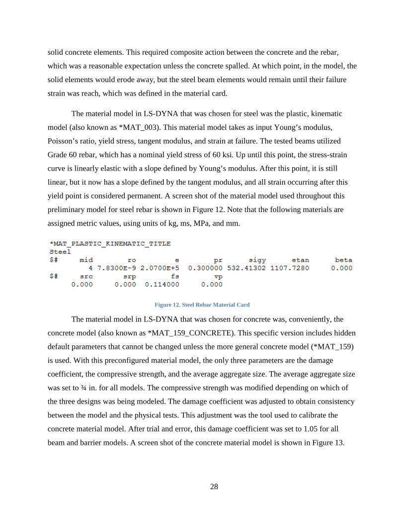
The material model in LS-DYNA that was chosen for steel was the plastic, kinematic

model (also known as *MAT_003). This material model takes as input Young’s modulus,

Poisson’s ratio, yield stress, tangent modulus, and strain at failure. The tested beams utilized

Grade 60 rebar, which has a nominal yield stress of 60 ksi. Up until this point, the stress-strain

curve is linearly elastic with a slope defined by Young’s modulus. After this point, it is still

linear, but it now has a slope defined by the tangent modulus, and all strain occurring after this

yield point is considered permanent. A screen shot of the material model used throughout this

preliminary model for steel rebar is shown in Figure 12. Note that the following materials are

assigned metric values, using units of kg, ms, MPa, and mm.

Figure 12. Steel Rebar Material Card

The material model in LS-DYNA that was chosen for concrete was, conveniently, the

concrete model (also known as *MAT_159_CONCRETE). This specific version includes hidden

default parameters that cannot be changed unless the more general concrete model (*MAT_159)

is used. With this preconfigured material model, the only three parameters are the damage

coefficient, the compressive strength, and the average aggregate size. The average aggregate size

was set to ¾ in. for all models. The compressive strength was modified depending on which of

the three designs was being modeled. The damage coefficient was adjusted to obtain consistency

between the model and the physical tests. This adjustment was the tool used to calibrate the

concrete material model. After trial and error, this damage coefficient was set to 1.05 for all

beam and barrier models. A screen shot of the concrete material model is shown in Figure 13.

29

Figure 13. Concrete Material Card

These two material models, and specifically the damage coefficient for the concrete

model, provided reasonably accurate fracture patterns in the simulated beam impact. Also, the

force-deflection curves were compared, and it was determined that the model provided

reasonable solutions for the three designs. An overhead view of the physical and virtual beams

for Design 3 is shown in Figure 14.

Figure 14. Design 3 Comparisons

The physical beams were impacted with the intent to fracture them, exceeding their

capacities. This allowed researchers to analyze the beams’ behaviors through the entire range of

strength. However, as can be noted in the models, many of the concrete elements became highly

distorted near the end of the simulation, at large displacements. Normally, this would be a

concern that should be rectified in order to create a robust material model. However, because this

30

was part of a preliminary comparison, and because the modified YLM was only concerned with

strains in the rebar of 6% or less, the material model behavior for larger strains was not

investigated further.

Internal Energy of Truck

The steel and concrete material models previously referenced were considered accurate

for small to moderate strains, including the 6-percent strain limit imposed in the modified YLM.

Therefore, the modeling effort proceeded by inserting these two material models into a full-scale

crash model involving a New Jersey bridge rail and an NCHRP 350 TL-4 vehicle (a single-unit

truck). The barrier model had 9 parts, 338,462 elements, and 345,519 nodes. The truck model

was downloaded from the NCAC model archive website [15]. It included 151 parts, 35,400

elements, and 38,949 nodes. It was given an initial velocity of 49.7 mph, and the bridge rail was

oriented such that the impact angle of the truck was 15 degrees. Other than initial conditions, the

truck model was unmodified, and details of the model can be found on the referenced website. A

screen shot of the orientation of the model is shown in Figure 15.

31

Figure 15. Impact Orientation of Bridge Rail Impact

The New Jersey bridge rail was modeled in a similar fashion as the concrete beams.

Concrete was discretized by solid elements, and rebar was discretized by discrete beam elements

that shared nodes with the concrete. A bridge deck overhang was also included. Steel stirrup

from the bridge rail extended down into the deck overhang, providing a connection between the

two concrete components. The total width of the modeled deck overhang was 39 inches, and the

remainder of the virtual bridge deck was modeled with a planar rigid wall in order to keep the

truck at deck level prior to impact. The element formulation and material cards were the same as

the beam model described in the previous section.

Energy calculations were the primary interest in the post processing of the model,

however barrier deflection, specifically in the rebar, was requisite for comparison to the modified

YLM. The deflections in the longitudinal rebar were tracked and used to calculate strains. When

the maximum rebar strain reached 6%, that time was flagged as 𝑡𝑡′. At 𝑡𝑡′, the energy levels were

investigated. Particularly, the internal energy due to the deformation of the vehicle was

investigated. The LS-PrePost post-processor was used to calculate this energy. Unfortunately, the

32

total internal energy of the truck was not a trivial number to report. Global calculations were

available through the GLSTAT ASCII file output, but this includes the internal energy of the

barrier system as well. Therefore, internal energies of selected parts were added together using

the ASCII file output from the MATSUM option in LS-DYNA. The total vehicle internal energy

was 17.9 kip-ft (11.9% or the impact severity, or IS). In contrast, the calculated internal energy

of the vehicle using the modified YLM was 20.5 kJ (13.7% of the IS).

33

6. DISCUSSION OF RESULTS

Deformation in the barrier and overhang system is an integral part in the crash event.

Generally, the specific deformation, and by extension energy absorption, of the barrier and

overhang system are not considered. Instead, it is assumed that the barrier is rigid, and that the

absorbed energy needed to redirect the vehicle is absorbed entirely by the vehicle. The modified

YLM was developed under the assumption that the momentum transfer between the vehicle and

the barrier/deck system was significant. Computer simulations support this belief when the

barrier and deck were modeled with deformable materials, rather than as rigid objects.

The ramification of this extra energy absorption is that the critical impact load imparted

on the barrier is reduced. The deformation of the wall also elicits an extended period of

attenuation of the vehicle’s velocity. Force can be tied to mass and velocity by way of the

impulse of the impact, which includes a consideration of the duration of the impact event. For

short-duration impacts, the force can be high, but if the duration is extended, the forces can be

lowered. A compliant barrier will have a longer duration of impact than a perfectly rigid barrier,

and as such, the expected loads imparted on the barrier from the vehicle will be lower if the

barrier is allowed to deform.

Barrier height also effects barrier compliance, and ultimately the load applied to the

barrier. The effect of barrier height is multi-faceted, but if the reinforcement design is constant

between two different height, the taller barrier will experience less load, including the barrier-

deck interface. The taller height creates a longer moment arm, which makes the barrier wall

weaker, allowing for more deformation and extending the impact event over a longer period. All

of this results in a lower transfer of load from the truck to the barrier. It also means that taller

barriers have less resistive capacity unless they are given more reinforcement than their shorter

counterparts. In general, a taller barrier is designed with more steel reinforcement since the

application of taller barriers generally coincides with larger vehicles. They are also more

susceptible to impacts with the cargo bed of the truck in secondary impacts, which may

contribute to the overall damage to the barrier. Tall barriers also help prevent vehicles from

rolling over the barrier. This does not necessarily contribute to the energy argument, but it an

important consideration when dealing with bridges.

34

Recent research has recommended increasing the AASHTO transverse design loads up to

93 kips for tall TL-4 barriers and either 160 kips or 260 kips to short or tall TL-5 barriers. These

elevated recommendations were likely due to the presence of the secondary impact, known

generally as tail slap. In particular, the cargo beds of the TL-4 and TL-5 vehicles made contact

with the top of the taller barriers in the computer simulations. However, in the experience of the

research team for the current project, this contact between the cargo bed and the top of a 36-inch

barrier does not occur. The distance from the ground to the top of the frame of the cargo bed is

typically 45 to 50 inches for a TL-4 test vehicle. A schematic of the dimensional drawing for a

TL-4 is shown in Figure 16, where the top of the frame of the cargo bed is labeled “l” on the far

right.

Figure 16. TL-4 Test Vehicle Dimensional Drawing

35

7. CONCLUSIONS AND RECOMMENDATIONS

The primary focus of the performance of concrete barriers has always been on the vehicle

dynamics after the impact. As such, a tendency in the modeling sector has been to establish the

shape of barrier and define it as a rigid object. This assists with reducing computational demands

from large models. However, it may not be an appropriate assumption for bridge rails, which use

less material through the cross section, such as with the New Jersey barrier. It is also install on

bridge overhang decks. The net result of these differences relative to standard median barriers is

a more compliant system. Since the system has mass, and is allowed to deform, it must, by

definition, absorb energy while undergoing this deformation. With a rigid assumption, this

absorbed energy is neglected.

During an impact, only a portion of the bridge rail moves, rather than the entire rail.

Nevertheless, because a portion of the rail moves after impact, the law of the conservation of

momentum applies. This law dictates that the masses of two separate objects traveling at

different speeds combine to move at the same speed. The mass of the bridge rail is determined by

what portion of the bridge rail moves. However, this determination is not trivial and requires

determining an effective length.

The modified YLM accounted for momentum transfer of the vehicle to a portion of the

barrier, and it included a consideration for the deformation of the barrier itself. With all of these

considerations, all FHWA-approved bridge rails for TL-4 and TL-5 were adequate when

compared to AASHTO’s current design transverse load of 54 kips. None of the crash tested

bridge rails experience significant damage at the base or through the height of the system.

The design loads corresponding to TL-4 and TL-5 have been the subject of debate lately

with the implementation of MASH as a replacement for NCHRP 350. The only difference in the

two for TL-4 was additional mass for the truck. TL-5 was not changed in any way. Recent

research has suggested that the AASHTO transverse design loads should be increased to as high

as 93 kips and 260 kips for TL-4 and TL-5, respectively, depending on the height of the barrier.

These numbers were based on complex computer simulations. However, the traditional YLM

was modified to included momentum transfer and barrier deformation, resulting in a less

demanding set of computations without sacrificing accuracy. With this modified YLM, a

36

historical bridge rail, crash tested in 1976, was evaluated because it exhibited structural failure

but still redirected the bus. This suggests that the barrier was very near its limit and capacity to

redirect the bus. Interpolating the impact severity between the TL-4 and TL-5 levels, the

interpolated design load (between 54 and 124 kips) would have been 91.8 kips. The capacity

according to the modified YLM was 92.1 kips, a 0.3% difference. This correlation suggests that

the modified YLM is accurate and that the AASHTO design loads, 54 and 124 kips, are

appropriate.

37

8. REFERENCES

1. Hirsch

2. AASHTO Bridge Specifications

3. NCHRP 350

4. MASH

5. TTI design loads

6. NCHRP 86

7. Steel rebar reference

8. FHWA website

9. Vertical Wall: http://guides.roadsafellc.com/Documents/SBC01d/Drawings/1993GSBH.pdf;

accessed: 12/18/2015.

10. Single Slope:

http://safety.fhwa.dot.gov/roadway_dept/policy_guide/road_hardware/barriers/bridgerailings/

docs/appendixb7g.pdf; accessed: 12/18/15

11. F-Shape:

http://safety.fhwa.dot.gov/roadway_dept/policy_guide/road_hardware/barriers/bridgerailings/

docs/appendixb7g.pdf; accessed: 12/18/15

12. NJ 32 – TTI Report

13. NJ 36 ref

14. NJ 42 ref

15. NCAC website

http://guides.roadsafellc.com/Documents/SBC01d/Drawings/1993GSBH.pdf

http://safety.fhwa.dot.gov/roadway_dept/policy_guide/road_hardware/barriers/bridgerailings/docs/appendixb7g.pdf




38

9. APPENDICES

39

A. Barrier Moment Capacity Calculations

40

1. Vertical Wall

Given:

𝑜𝑜𝑦𝑦 = 60 𝑘𝑘𝑠𝑠𝑖𝑖 (A.1.1)

𝑜𝑜𝑐𝑐′ = 3.6 𝑘𝑘𝑠𝑠𝑖𝑖 (A.1.2)

Rebar size: #8 (A.1.3)

𝐴𝐴𝑠𝑠 = 0.79 𝑖𝑖𝑖𝑖2 𝑝𝑝𝐵𝐵𝐵𝐵 𝑏𝑏𝑎𝑎𝐵𝐵 (A.1.4)

Beam width: 𝑏𝑏 = 8.86 𝑖𝑖𝑖𝑖 (A.1.5)

Beam depth: 𝐷𝐷𝑏𝑏 = 12 𝑖𝑖𝑖𝑖 (A.1.6)

Cover: 𝑑𝑑𝑐𝑐 = 1.5748 𝑖𝑖𝑖𝑖 (A.1.7)

Bars in beam: 𝑖𝑖𝑏𝑏 = 2 (A.1.8)

Bars in wall: 𝑖𝑖𝑤𝑤 = 4 (A.1.9)

Wall height: ℎ = 33.27 𝑖𝑖𝑖𝑖 (A.1.10)

Wall depth: 𝐷𝐷𝑤𝑤 = 10.43 𝑖𝑖𝑖𝑖 (A.1.11)

Stirrup size: #5 (A.1.12)

Stirrup spacing: 𝑠𝑠 = 11.811 𝑖𝑖𝑖𝑖 (A.1.13)

Beam Moment:

𝑎𝑎 = 𝑛𝑛𝑏𝑏𝐴𝐴𝑠𝑠𝑓𝑓𝑦𝑦𝛽𝛽1𝑓𝑓𝑐𝑐′𝑏𝑏

= (2)(0.79)(60)(0.85)(3.6)(8.86)

= 3.4967 𝑖𝑖𝑖𝑖 (A.1.14)

𝑑𝑑𝑏𝑏 = 𝐷𝐷𝑏𝑏 − 𝑑𝑑𝑐𝑐 − 58� − 0.5�8

8� � = 9.3 𝑖𝑖𝑖𝑖 (A.1.15)

𝑀𝑀𝑁𝑁 = 𝑖𝑖𝑏𝑏𝐴𝐴𝑠𝑠𝑜𝑜𝑦𝑦 �𝑑𝑑𝑏𝑏 −𝑙𝑙2� = (2)(0.79)(60) �9.3 − 3.4967

2� = 715.92 𝑘𝑘𝑖𝑖𝑝𝑝 − 𝑖𝑖𝑖𝑖 (A.1.16)

𝑀𝑀𝑏𝑏 = 𝑀𝑀𝑁𝑁12

= 59.66 𝑘𝑘𝑖𝑖𝑝𝑝 − 𝑜𝑜𝑡𝑡 (A.1.17)

Wall Moment:


= (4)(0.79)(60)(0.85)(3.6)(33.27)

= 1.86236 𝑖𝑖𝑖𝑖 (A.1.18)

𝑑𝑑𝑤𝑤 = 𝐷𝐷𝑤𝑤 − 𝑑𝑑𝑐𝑐 − 58� − 0.5�8

8� � = 7.7 𝑖𝑖𝑖𝑖 (A.1.19)

𝑀𝑀𝑁𝑁 = 𝑖𝑖𝑏𝑏𝐴𝐴𝑠𝑠𝑜𝑜𝑦𝑦 �𝑑𝑑 −𝑙𝑙2� = (4)(0.79)(60) �7.7 − 1.86236

2� = 1,289.68 𝑘𝑘𝑖𝑖𝑝𝑝 − 𝑖𝑖𝑖𝑖 (A.1.20)

𝑀𝑀𝑤𝑤 = 𝑀𝑀𝑁𝑁ℎ

= 38.76 𝑘𝑘𝑖𝑖𝑘𝑘−𝑓𝑓𝑙𝑙𝑓𝑓𝑙𝑙

(A.1.21)

41

Cantilever Moment:


= (1)(0.31)(60)(0.85)(3.6)(11.811)

= 0.514642 𝑖𝑖𝑖𝑖 (A.1.22)

𝑑𝑑𝑐𝑐 = 𝐷𝐷𝑤𝑤 − 𝑑𝑑𝑐𝑐 − 0.5�58� � = 8.55 𝑖𝑖𝑖𝑖 (A.1.23)

𝑀𝑀𝑁𝑁 = 𝐴𝐴𝑠𝑠𝑜𝑜𝑦𝑦 �𝑑𝑑 −𝑙𝑙2� = (0.31)(60) �8.55 − 0.514642

2� = 154.17 𝑘𝑘𝑖𝑖𝑝𝑝 − 𝑖𝑖𝑖𝑖 (A.1.24)

𝑀𝑀𝑤𝑤 = 𝑀𝑀𝑁𝑁𝑠𝑠


(A.1.25)

2. Single Slope

Given:





Top width: 𝑏𝑏𝑙𝑙 = 9.5 𝑖𝑖𝑖𝑖 (A.2.5)

Bottom width: 𝑏𝑏𝑏𝑏 = 15.675 𝑖𝑖𝑖𝑖 (A.2.6)



Wall height: ℎ = 32 𝑖𝑖𝑖𝑖 (A.2.9)


Stirrup spacing: 𝑠𝑠 = 8 𝑖𝑖𝑖𝑖 (A.2.11)

Slope of face: 𝛼𝛼 = 10.8 𝑑𝑑𝐵𝐵𝑎𝑎𝐵𝐵𝐵𝐵𝐵𝐵𝑠𝑠 (A.2.12)

Beam Moment:

𝑀𝑀𝑏𝑏 = 0 𝑘𝑘𝑖𝑖𝑝𝑝 − 𝑜𝑜𝑡𝑡 (A.2.13)

Wall Moment:


= (4)(0.20)(60)(0.85)(4.0)(32)

= 0.415225 𝑖𝑖𝑖𝑖 (A.2.14)

𝐷𝐷1 = 𝑏𝑏𝑙𝑙 − ℎ1 tan 10.8 = 9.5 + (1.75)(0.19076) = 9.83383 𝑖𝑖𝑖𝑖 (A.2.15)


42


𝐷𝐷4 = 𝑏𝑏𝑙𝑙 − ℎ4 tan 10.8 = 9.5 + (25)(0.19076) = 14.269 𝑖𝑖𝑖𝑖 (A.2.18)

𝑑𝑑𝑙𝑙𝑎𝑎𝑔𝑔 = ∑(𝐷𝐷𝑖𝑖−1.5−0.5∙0.625)4

= 10.2389 𝑖𝑖𝑖𝑖 (A.2.19)

𝑀𝑀𝑁𝑁 = 𝑖𝑖𝑤𝑤𝐴𝐴𝑠𝑠𝑜𝑜𝑦𝑦 �𝑑𝑑 −𝑙𝑙2� = (4)(0.20)(60) �10.2389 − 0.415225

2� = 481.502 𝑘𝑘 − 𝑖𝑖𝑖𝑖 (A.2.20)



(A.2.21)

Cantilever Moment:


= (1)(0.31)(60)(0.85)(4.0)(8)

= 0.683824 𝑖𝑖𝑖𝑖 (A.2.22)

𝑑𝑑𝑐𝑐 = 𝑏𝑏𝑏𝑏 − 𝑑𝑑𝑐𝑐 − 0.5�58� � = 13.8125 𝑖𝑖𝑖𝑖 (A.2.23)


2� = 250.553 𝑘𝑘 − 𝑖𝑖𝑖𝑖 (A.2.24)

𝑀𝑀𝑐𝑐 = 𝑀𝑀𝑁𝑁𝑠𝑠


(A.2.25)

43

3. F-Shape

Given:











Stirrup clearance: 𝑑𝑑𝑠𝑠 = 3 𝑖𝑖𝑖𝑖 (A.3.11)


Slope of face: 𝛼𝛼 = 6.02066 𝑑𝑑𝐵𝐵𝑎𝑎𝐵𝐵𝐵𝐵𝐵𝐵𝑠𝑠 (A.3.13)

Beam Moment:


Wall Moment:


= (4)(0.60)(40)(0.85)(3.6)(42)

= 0.746965 𝑖𝑖𝑖𝑖 (A.3.15)

𝐷𝐷1 = 𝑏𝑏𝑙𝑙 + ℎ1 tan 6.02 = 9.0 + (3)(0.105469) = 9.31641 𝑖𝑖𝑖𝑖 (A.3.16)

𝐷𝐷2 = 𝑏𝑏𝑙𝑙 + ℎ2 tan 6.02 = 9.0 + (12)(0.105469) = 10.2656 𝑖𝑖𝑖𝑖 (A.3.17)

𝐷𝐷3 = 𝑏𝑏𝑙𝑙 + ℎ3 tan 6.02 = 9.0 + (22)(0.105469) − 1.5 = 9.82031 𝑖𝑖𝑖𝑖 (A.3.18)

𝐷𝐷4 = 𝑏𝑏𝑙𝑙 + ℎ4 tan 6.02 = 9.0 + (32)(0.105469) − 1.5 = 10.875 𝑖𝑖𝑖𝑖 (A.3.19)

𝑑𝑑𝑙𝑙𝑎𝑎𝑔𝑔 = ∑(𝐷𝐷𝑖𝑖−1.5−0.5∙0.625)4

= 8.25683 𝑖𝑖𝑖𝑖 (A.3.20)

𝑀𝑀𝑁𝑁 = 𝑖𝑖𝑤𝑤𝐴𝐴𝑠𝑠𝑜𝑜𝑦𝑦 �𝑑𝑑 −𝑙𝑙2� = (4)(0.60)(40) �8.25683 − 0.746965

2� = 756.801 𝑘𝑘 − 𝑖𝑖𝑖𝑖 (A.3.21)



(A.3.22)

44

Cantilever Moment:


= (1)(0.31)(40)(0.85)(3.6)(8)

= 0.506536 𝑖𝑖𝑖𝑖 (A.3.23)

𝑑𝑑𝑐𝑐 = 𝑏𝑏𝑏𝑏 − 𝑑𝑑𝑠𝑠 − 0.5�58� � = 13.9375 𝑖𝑖𝑖𝑖 (A.3.24)


2� = 169.684 𝑘𝑘 − 𝑖𝑖𝑖𝑖 (A.3.25)

𝑀𝑀𝑐𝑐 = 𝑀𝑀𝑁𝑁𝑠𝑠


(A.3.26)

45

4. New Jersey Shape – 32”

Given:






Bottom width: 𝑏𝑏𝑏𝑏 = 15 𝑖𝑖𝑖𝑖 (A.4.6)







Slope of top face: 𝛼𝛼 = 6.00901 𝑑𝑑𝐵𝐵𝑎𝑎𝐵𝐵𝐵𝐵𝐵𝐵𝑠𝑠 (A.4.13)

Slope of bottom face: 𝛾𝛾 = 34.992 𝑑𝑑𝐵𝐵𝑎𝑎𝐵𝐵𝐵𝐵𝐵𝐵𝑠𝑠 (A.4.14)

Beam Moment:


Wall Moment:


= (4)(0.20)(60)(0.85)(3.6)(32)

= 0.490196 𝑖𝑖𝑖𝑖 (A.4.16)

Backside

𝑑𝑑1 = 𝑏𝑏𝑙𝑙 + (2) tan 6.01 − 1.8125 = 4.37171 𝑖𝑖𝑖𝑖 (A.4.17)

𝑑𝑑2 = 𝑏𝑏𝑙𝑙 + (10) tan 6.01 − 1.8125 = 5.1875 𝑖𝑖𝑖𝑖 (A.4.18)

𝑑𝑑3 = 𝑏𝑏𝑙𝑙 + (18) tan 6.01 − 1.8125 = 6.00329 𝑖𝑖𝑖𝑖 (A.4.19)

𝑑𝑑4 = 𝑏𝑏𝑙𝑙 + (26) tan 6.01 − 1.8125 = 8.7373 𝑖𝑖𝑖𝑖 (A.4.20)

𝑀𝑀1 = 𝐴𝐴𝑠𝑠𝑜𝑜𝑦𝑦 �𝑑𝑑1 −𝑙𝑙2� = (0.20)(60) �4.37171 − 0.490196

2� = 49.52 𝑘𝑘 − 𝑖𝑖𝑖𝑖 (A.4.21)

𝑀𝑀2 = 𝐴𝐴𝑠𝑠𝑜𝑜𝑦𝑦 �𝑑𝑑2 −𝑙𝑙2� = (0.20)(60) �5.1875 − 0.490196

2� = 59.31 𝑘𝑘 − 𝑖𝑖𝑖𝑖 (A.4.22)

46

𝑀𝑀3 = 𝐴𝐴𝑠𝑠𝑜𝑜𝑦𝑦 �𝑑𝑑3 −𝑙𝑙2� = (0.20)(60) �6.00329 − 0.490196

2� = 69.10 𝑘𝑘 − 𝑖𝑖𝑖𝑖 (A.4.23)

𝑀𝑀4 = 𝐴𝐴𝑠𝑠𝑜𝑜𝑦𝑦 �𝑑𝑑4 −𝑙𝑙2� = (0.20)(60) �8.2875 − 0.490196

2� = 101.91 𝑘𝑘 − 𝑖𝑖𝑖𝑖 (A.4.24)

𝑀𝑀𝑁𝑁 = ∑𝑀𝑀𝑖𝑖 = 279.83 𝑘𝑘𝑖𝑖𝑝𝑝 − 𝑖𝑖𝑖𝑖 (A.4.25)

Frontside

𝑑𝑑1 = 𝑏𝑏𝑙𝑙 + ℎ1 tan 6.01 − 1.8125 = 4.37171 𝑖𝑖𝑖𝑖 (A.4.26)



𝑑𝑑4 = �𝑑𝑑3−𝑑𝑑115.5

� (7.75) + 𝑑𝑑3 = 6.81908 𝑖𝑖𝑖𝑖 (A.4.29)

𝑀𝑀1 = 𝐴𝐴𝑠𝑠𝑜𝑜𝑦𝑦 �𝑑𝑑1 −𝑙𝑙2� = (0.20)(60) �4.37171 − 0.490196

2� = 49.52 𝑘𝑘 − 𝑖𝑖𝑖𝑖 (A.4.30)

𝑀𝑀2 = 𝐴𝐴𝑠𝑠𝑜𝑜𝑦𝑦 �𝑑𝑑2 −𝑙𝑙2� = (0.20)(60) �5.1875 − 0.490196

2� = 59.31 𝑘𝑘 − 𝑖𝑖𝑖𝑖 (A.4.31)

𝑀𝑀3 = 𝐴𝐴𝑠𝑠𝑜𝑜𝑦𝑦 �𝑑𝑑3 −𝑙𝑙2� = (0.20)(60) �6.00329 − 0.490196

2� = 69.10 𝑘𝑘 − 𝑖𝑖𝑖𝑖 (A.4.32)

𝑀𝑀4 = 𝐴𝐴𝑠𝑠𝑜𝑜𝑦𝑦 �𝑑𝑑4 −𝑙𝑙2� = (0.20)(60) �6.81908 − 0.490196

2� = 78.89 𝑘𝑘 − 𝑖𝑖𝑖𝑖 (A.4.33)


𝑀𝑀𝑤𝑤 = min𝑀𝑀𝑁𝑁ℎ

= 256.8132


(A.4.35)

Cantilever Moment:


= (1)(0.31)(60)(0.85)(3.6)(8)

= 0.759804 𝑖𝑖𝑖𝑖 (A.4.36)

Bottom Section

𝑑𝑑𝑐𝑐 = 15 − 2.86 = 11.2378 𝑖𝑖𝑖𝑖 (A.4.37)


2� = 201.96 𝑘𝑘 − 𝑖𝑖𝑖𝑖 (A.4.38)

Top Section

𝑑𝑑𝑐𝑐 = 5.35598 𝑖𝑖𝑖𝑖 (A.4.39)


2� = 92.56 𝑘𝑘 − 𝑖𝑖𝑖𝑖 (A.4.40)

𝑀𝑀𝑐𝑐 = min 𝑀𝑀𝑁𝑁𝑠𝑠

= 92.568


(A.4.41)

47


Given:















Beam Moment:


Wall Moment:


= (4)(0.20)(60)(0.85)(3.6)(36)

= 0.43573 𝑖𝑖𝑖𝑖 (A.5.16)

Backside

𝑑𝑑1 = 𝑏𝑏𝑙𝑙 + (2) tan 4.97 − 1.8125 = 4.3614 𝑖𝑖𝑖𝑖 (A.5.17)

𝑑𝑑2 = 𝑏𝑏𝑙𝑙 + (12) tan 4.97 − 1.8125 = 5.2310 𝑖𝑖𝑖𝑖 (A.5.18)

𝑑𝑑3 = 𝑏𝑏𝑙𝑙 + (22) tan 4.97 − 1.8125 = 6.1005 𝑖𝑖𝑖𝑖 (A.5.19)

𝑑𝑑4 = 𝑏𝑏𝑙𝑙 + (30) tan 4.97 − 1.8125 = 6.7962 𝑖𝑖𝑖𝑖 (A.5.20)

𝑀𝑀1 = 𝐴𝐴𝑠𝑠𝑜𝑜𝑦𝑦 �𝑑𝑑1 −𝑙𝑙2� = (0.20)(60) �4.3614 − 0.43573

2� = 49.72 𝑘𝑘 − 𝑖𝑖𝑖𝑖 (A.5.21)

𝑀𝑀2 = 𝐴𝐴𝑠𝑠𝑜𝑜𝑦𝑦 �𝑑𝑑2 −𝑙𝑙2� = (0.20)(60) �5.2310 − 0.43573

2� = 60.16 𝑘𝑘 − 𝑖𝑖𝑖𝑖 (A.5.22)

48

𝑀𝑀3 = 𝐴𝐴𝑠𝑠𝑜𝑜𝑦𝑦 �𝑑𝑑3 −𝑙𝑙2� = (0.20)(60) �6.1005 − 0.43573

2� = 70.59 𝑘𝑘 − 𝑖𝑖𝑖𝑖 (A.5.23)

𝑀𝑀4 = 𝐴𝐴𝑠𝑠𝑜𝑜𝑦𝑦 �𝑑𝑑4 −𝑙𝑙2� = (0.20)(60) �6.7962 − 0.43573

2� = 78.94 𝑘𝑘 − 𝑖𝑖𝑖𝑖 (A.5.24)


Frontside

𝑑𝑑1 = 𝑏𝑏𝑙𝑙 + (2) tan 4.97 − 1.8125 = 4.3614 𝑖𝑖𝑖𝑖 (A.5.26)

𝑑𝑑2 = 𝑏𝑏𝑙𝑙 + (12) tan 4.97 − 1.8125 = 5.2310 𝑖𝑖𝑖𝑖 (A.5.27)

𝑑𝑑3 = 𝑏𝑏𝑙𝑙 + (22) tan 4.97 − 1.8125 = 6.1005 𝑖𝑖𝑖𝑖 (A.5.28)

𝑑𝑑4 = 15 − � 310� (7) − 1.8125 = 11.0875 𝑖𝑖𝑖𝑖 (A.5.29)

𝑀𝑀1 = 𝐴𝐴𝑠𝑠𝑜𝑜𝑦𝑦 �𝑑𝑑1 −𝑙𝑙2� = (0.20)(60) �4.3614 − 0.43573

2� = 49.72 𝑘𝑘 − 𝑖𝑖𝑖𝑖 (A.5.30)

𝑀𝑀2 = 𝐴𝐴𝑠𝑠𝑜𝑜𝑦𝑦 �𝑑𝑑2 −𝑙𝑙2� = (0.20)(60) �5.2310 − 0.43573

2� = 60.16 𝑘𝑘 − 𝑖𝑖𝑖𝑖 (A.5.31)

𝑀𝑀3 = 𝐴𝐴𝑠𝑠𝑜𝑜𝑦𝑦 �𝑑𝑑3 −𝑙𝑙2� = (0.20)(60) �6.1005 − 0.43573

2� = 70.59 𝑘𝑘 − 𝑖𝑖𝑖𝑖 (A.5.32)

𝑀𝑀4 = 𝐴𝐴𝑠𝑠𝑜𝑜𝑦𝑦 �𝑑𝑑4 −𝑙𝑙2� = (0.20)(60) �11.0875 − 0.43573

2� = 130.44 𝑘𝑘 − 𝑖𝑖𝑖𝑖 (A.5.33)



= 259.4136


(A.5.35)

Cantilever Moment:


= (1)(0.31)(60)(0.85)(3.6)(8)

= 0.759804 𝑖𝑖𝑖𝑖 (A.5.36)

Bottom Section

𝑑𝑑𝑐𝑐 = 15 − 2.86 = 11.2378 𝑖𝑖𝑖𝑖 (A.5.37)


2� = 201.96 𝑘𝑘 − 𝑖𝑖𝑖𝑖 (A.5.38)

Top Section

𝑑𝑑𝑐𝑐 = 5.35598 𝑖𝑖𝑖𝑖 (A.5.39)


2� = 92.56 𝑘𝑘 − 𝑖𝑖𝑖𝑖 (A.5.40)


= 92.568


(A.5.41)

49


Given:















Beam Moment:


Wall Moment:


= (5)(0.20)(60)(0.85)(3.6)(42)

= 0.466853 𝑖𝑖𝑖𝑖 (A.6.16)

Backside

𝑑𝑑1 = 𝑏𝑏𝑙𝑙 + (2) tan 3.95 − 1.8125 = 4.3254 𝑖𝑖𝑖𝑖 (A.6.17)

𝑑𝑑2 = 𝑏𝑏𝑙𝑙 + (10.25) tan 3.95 − 1.8125 = 4.8944 𝑖𝑖𝑖𝑖 (A.6.18)

𝑑𝑑3 = 𝑏𝑏𝑙𝑙 + (18.5) tan 3.95 − 1.8125 = 5.4634 𝑖𝑖𝑖𝑖 (A.6.19)

𝑑𝑑4 = 𝑏𝑏𝑙𝑙 + (26.75) tan 3.95 − 1.8125 = 6.0323 𝑖𝑖𝑖𝑖 (A.6.20)

𝑑𝑑5 = 𝑏𝑏𝑙𝑙 + (35) tan 3.95 − 1.8125 = 6.6013 𝑖𝑖𝑖𝑖 (A.6.21)

𝑀𝑀1 = 𝐴𝐴𝑠𝑠𝑜𝑜𝑦𝑦 �𝑑𝑑1 −𝑙𝑙2� = (0.20)(60) �4.3254 − 0.466853

2� = 49.10 𝑘𝑘 − 𝑖𝑖𝑖𝑖 (A.6.22)

50

𝑀𝑀2 = 𝐴𝐴𝑠𝑠𝑜𝑜𝑦𝑦 �𝑑𝑑2 −𝑙𝑙2� = (0.20)(60) �4.8944 − 0.466853

2� = 55.93 𝑘𝑘 − 𝑖𝑖𝑖𝑖 (A.6.23)

𝑀𝑀3 = 𝐴𝐴𝑠𝑠𝑜𝑜𝑦𝑦 �𝑑𝑑3 −𝑙𝑙2� = (0.20)(60) �5.4634 − 0.466853

2� = 62.76 𝑘𝑘 − 𝑖𝑖𝑖𝑖 (A.6.24)

𝑀𝑀4 = 𝐴𝐴𝑠𝑠𝑜𝑜𝑦𝑦 �𝑑𝑑4 −𝑙𝑙2� = (0.20)(60) �6.0323 − 0.466853

2� = 69.59 𝑘𝑘 − 𝑖𝑖𝑖𝑖 (A.6.25)

𝑀𝑀5 = 𝐴𝐴𝑠𝑠𝑜𝑜𝑦𝑦 �𝑑𝑑5 −𝑙𝑙2� = (0.20)(60) �6.6013 − 0.466853

2� = 76.41 𝑘𝑘 − 𝑖𝑖𝑖𝑖 (A.6.26)


Frontside

𝑑𝑑1 = 𝑏𝑏𝑙𝑙 + (2) tan 3.95 − 1.8125 = 4.3254 𝑖𝑖𝑖𝑖 (A.6.28)

𝑑𝑑2 = 𝑏𝑏𝑙𝑙 + (10.25) tan 3.95 − 1.8125 = 4.8944 𝑖𝑖𝑖𝑖 (A.6.29)

𝑑𝑑3 = 𝑏𝑏𝑙𝑙 + (18.5) tan 3.95 − 1.8125 = 5.4634 𝑖𝑖𝑖𝑖 (A.6.30)

𝑑𝑑4 = 𝑏𝑏𝑙𝑙 + (26.75) tan 3.95 − 1.8125 = 6.0323 𝑖𝑖𝑖𝑖 (A.6.31)

𝑑𝑑5 = 15 − �3.80410

� (7) − 1.8125 = 10.525 𝑖𝑖𝑖𝑖 (A.6.32)

𝑀𝑀1 = 𝐴𝐴𝑠𝑠𝑜𝑜𝑦𝑦 �𝑑𝑑1 −𝑙𝑙2� = (0.20)(60) �4.3254 − 0.466853

2� = 49.10 𝑘𝑘 − 𝑖𝑖𝑖𝑖 (A.6.33)

𝑀𝑀2 = 𝐴𝐴𝑠𝑠𝑜𝑜𝑦𝑦 �𝑑𝑑2 −𝑙𝑙2� = (0.20)(60) �4.8944 − 0.466853

2� = 55.93 𝑘𝑘 − 𝑖𝑖𝑖𝑖 (A.6.34)

𝑀𝑀3 = 𝐴𝐴𝑠𝑠𝑜𝑜𝑦𝑦 �𝑑𝑑3 −𝑙𝑙2� = (0.20)(60) �5.4634 − 0.466853

2� = 62.76 𝑘𝑘 − 𝑖𝑖𝑖𝑖 (A.6.35)

𝑀𝑀4 = 𝐴𝐴𝑠𝑠𝑜𝑜𝑦𝑦 �𝑑𝑑4 −𝑙𝑙2� = (0.20)(60) �6.0323 − 0.466853

2� = 69.59 𝑘𝑘 − 𝑖𝑖𝑖𝑖 (A.6.36)

𝑀𝑀5 = 𝐴𝐴𝑠𝑠𝑜𝑜𝑦𝑦 �𝑑𝑑5 −𝑙𝑙2� = (0.20)(60) �10.525 − 0.466853

2� = 123.50 𝑘𝑘 − 𝑖𝑖𝑖𝑖 (A.6.37)



= 313.8042


(A.6.39)

Cantilever Moment:


= (1)(0.31)(60)(0.85)(3.6)(8)

= 0.759804 𝑖𝑖𝑖𝑖 (A.6.40)

Bottom Section

𝑑𝑑𝑐𝑐 = 15 − 2.86 = 11.2378 𝑖𝑖𝑖𝑖 (A.6.41)


2� = 201.96 𝑘𝑘 − 𝑖𝑖𝑖𝑖 (A.6.42)

Top Section

𝑑𝑑𝑐𝑐 = 5.35598 𝑖𝑖𝑖𝑖 (A.6.43)

51


2� = 92.56 𝑘𝑘 − 𝑖𝑖𝑖𝑖 (A.6.44)


= 92.568


(A.6.45)

52


Given:















Beam Moment:


Wall Moment:


= (7)(0.31)(60)(0.85)(3.6)(54)

= 0.779801 𝑖𝑖𝑖𝑖 (A.6.16)

Backside

𝑑𝑑1 = 6.5 𝑖𝑖𝑖𝑖 (A.6.17)

𝑑𝑑2 = 6.86 𝑖𝑖𝑖𝑖 (A.6.18)

𝑑𝑑3 = 7.4 𝑖𝑖𝑖𝑖 (A.6.19)

𝑑𝑑4 = 7.76 𝑖𝑖𝑖𝑖 (A.6.20)

𝑑𝑑5 = 8.12 𝑖𝑖𝑖𝑖 (A.6.21)

𝑑𝑑6 = 8.48 𝑖𝑖𝑖𝑖 (A.6.20)

𝑑𝑑7 = 9.2 𝑖𝑖𝑖𝑖 (A.6.21)

53

𝑀𝑀1 = 𝐴𝐴𝑠𝑠𝑜𝑜𝑦𝑦 �𝑑𝑑1 −𝑙𝑙2� = (0.20)(60) �6.5 − 0.779801

2� = 112.47 𝑘𝑘 − 𝑖𝑖𝑖𝑖 (A.6.22)

𝑀𝑀2 = 𝐴𝐴𝑠𝑠𝑜𝑜𝑦𝑦 �𝑑𝑑2 −𝑙𝑙2� = (0.20)(60) �6.86 − 0.779801

2� = 119.10 𝑘𝑘 − 𝑖𝑖𝑖𝑖 (A.6.23)

𝑀𝑀3 = 𝐴𝐴𝑠𝑠𝑜𝑜𝑦𝑦 �𝑑𝑑3 −𝑙𝑙2� = (0.20)(60) �7.4 − 0.779801

2� = 129.04 𝑘𝑘 − 𝑖𝑖𝑖𝑖 (A.6.24)

𝑀𝑀4 = 𝐴𝐴𝑠𝑠𝑜𝑜𝑦𝑦 �𝑑𝑑4 −𝑙𝑙2� = (0.20)(60) �7.76 − 0.779801

2� = 135.67 𝑘𝑘 − 𝑖𝑖𝑖𝑖 (A.6.25)

𝑀𝑀5 = 𝐴𝐴𝑠𝑠𝑜𝑜𝑦𝑦 �𝑑𝑑5 −𝑙𝑙2� = (0.20)(60) �8.12 − 0.779801

2� = 142.29 𝑘𝑘 − 𝑖𝑖𝑖𝑖 (A.6.26)

𝑀𝑀6 = 𝐴𝐴𝑠𝑠𝑜𝑜𝑦𝑦 �𝑑𝑑4 −𝑙𝑙2� = (0.20)(60) �8.48 − 0.779801

2� = 148.92 𝑘𝑘 − 𝑖𝑖𝑖𝑖 (A.6.25)

𝑀𝑀7 = 𝐴𝐴𝑠𝑠𝑜𝑜𝑦𝑦 �𝑑𝑑5 −𝑙𝑙2� = (0.20)(60) �9.2 − 0.779801

2� = 162.17 𝑘𝑘 − 𝑖𝑖𝑖𝑖 (A.6.26)


Frontside

𝑑𝑑7 = 13.7 𝑖𝑖𝑖𝑖 (A.7..)

𝑀𝑀7 = 𝐴𝐴𝑠𝑠𝑜𝑜𝑦𝑦 �𝑑𝑑5 −𝑙𝑙2� = (0.20)(60) �13.7 − 0.779801

2� = 245.01 𝑘𝑘 − 𝑖𝑖𝑖𝑖 (A.6.26)

𝑀𝑀𝑁𝑁 = ∑𝑀𝑀𝑖𝑖 = 1,032.51 𝑘𝑘𝑖𝑖𝑝𝑝 − 𝑖𝑖𝑖𝑖 (A.6.38)


= 949.6754


(A.6.39)

Cantilever Moment:

𝑎𝑎 = 𝐴𝐴𝑠𝑠𝑓𝑓𝑦𝑦𝛽𝛽1𝑓𝑓𝑐𝑐′𝑏𝑏

= (0.31)(60)(0.85)(3.6)(12)

= 0.506536 𝑖𝑖𝑖𝑖 (A.6.40)

Bottom Section

𝑑𝑑𝑐𝑐 = 9.8 𝑖𝑖𝑖𝑖 (A.6.41)


2� = 177.57 𝑘𝑘 − 𝑖𝑖𝑖𝑖 (A.6.42)

Top Section

𝑑𝑑𝑐𝑐 = 8.48 𝑖𝑖𝑖𝑖 (A.6.43)


2� = 151.44 𝑘𝑘 − 𝑖𝑖𝑖𝑖 (A.6.44)


= 151.4412


(A.6.45)

54

END OF DOCUMENT

Evaluation of Design Loads for Concrete Bridge Rails

Documents

Transcript of Evaluation of Design Loads for Concrete Bridge Rails