EVALUATION OF CELLULAR PREDICTION MODELS USING 900 MHz OUTDOOR MEASUREMENTS AND TUNING OF LEE MODEL OVER INDIAN URBAN & SUBURBAN REGIONS M V S N Prasad1 , K Ratnamala 2, P K Dalela3, Chandra Shekhar Misra4,

1. National Physical Laboratory, Dr. K S Krishnan road, New Delhi, India, e-mail: mvsnprasad@gmail.com, mvprasad@mail.nplindia.org

2. National Geophysical Research Institute, Hyderabad, India, email: kunala_ratnamala@rediffmail.com

3. C-DOT, Chattarpur, Mehraulli, New Delhi, India, email: pdalela@gmail.com 4. Aircom International Pvt Ltd., Gurgaon, India, email:

chandra.misra@aircom.co.uk

Abstract:

The present study reports the field strength measurements of some GSM transmitters in

the 900 MHz band located in the urban and suburban regions of Delhi in India. The

measured signal levels converted into path loss values have been compared with the

losses predicted from models like Hata, Lee and COST 231 Walfisch & Ikegami. The

prediction errors and standard deviations of the predictions errors have been deduced.

Based on these results, Lee prediction method has been tuned and new model parameters

have been derived. The model comparison is done in terms of statistical parameters like,

root mean square error, coefficient of determination and average hit rate error.

Key words: 900 MHz measurements, path loss modeling, Lee model tuning

1 Introduction

Due to the rapid developments in cellular communication over this country and the pace

with which the cellular data base is increasing, the standard 900 and 1800 MHz spectral

bands are becoming increasingly congested with the demands of more frequency

allocation by many operators. An efficient spectral allocation requires the testing of

various prediction methods. The evaluation of the prediction methods also helps to

determine the interference levels and help in electromagnetic interference and

compatibility studies. The 3G communication systems ready to be launched at any time

in the country also require good field trials and identification of coverage prediction

methods. In the past measurements in the 800/900 MHz band have been reported by

workers [1] and they tried to explain the extensive field results through theoretical

analysis and modeling of the physical phenomena. Some of the well known mobile

operators utilized calibrated statistical models for coverage and planning purposes

derived from Okumara-Hata model [2-3]. Vieira et al [4] extensively discussed the re-

farming of 900 MHz band into HSPA and LTE and stressed the importance of this band

for rural mobile broadband applications. The Lee propagation model has been recognized

by the wireless industry as one of the most accurate propagation model in the 900 MHz

band [5] wherein the authors Lee & Lee discussed several innovative and revolutionary

approaches that can better handle issues created by rough terrain sampling data.

The special feature in Delhi urban environment is most of the buildings are non

uniformly spaced and results reported elsewhere might not be totally applicable to this

type of environment. With this background and to evaluate the suitability of the existing

models, field strength measurements were conducted in the 900 MHz band utilizing the

following GSM base stations situated in national capital region of Delhi. They are

1.Paschimvihar (PVR) 2. University Area (UA) 3. Nandanagari -1 (NN-1). 4.

Nandanagari- 2 (NN-2) 5. Satyaniketan (SNT) 6. Faridabad (FBD) 7. Vinayak

Hospital (VKH) and three suburban base stations namely 1. Tradex tower (TXT), 2.

Meethapur (MPR) 3. Gurgaon (GRN). All the base stations shown on google earth map

are in figure 1 and figures 2a-2c show the map depicting the measurement route for three

base stations. These have been incorporated to get a feel of the environment for the

reader. The measured values of signal strength have been compared with the following

prediction methods 1. Hata [4] 2. Lee [5-6] 3. COST 231 Walfisch & Ikegami [7]. The

models have been chosen so that they are applicable to the environments where

measurements were conducted. An attempt is also made to tune the Lee method based on

the measured values. This type of work is the first of its kind from this region of the

world.

2 Environmental descriptions

Both the NN-1 and NN-2 base stations are surrounded by dense urban areas on three

sides and medium urban environment on the other side. The average building height is

around 6 to 9 m. PVR base station is surrounded by medium urban environment with

slight open areas in between. Far away from the base station on the left side low tree

density is seen. On the southern side of the base station a small water canal flows. UA

base station is surrounded by medium urban environment and from east to south of the

base station a thick patch of tree density is seen. At distances 2 km away from the base

station dense urban environment prevails on the southern side of the base station. MPR

base station is surrounded by low density urban area (mainly suburban) and small patches

of green vegetation in between. SNT base station is surrounded by medium urban

environment and small patches of greenery in between denoting some kind of low urban

residential environment. Clutter features of NN-1 and UA base station are shown in

figures 3 and 4 to get a glimpse of measurement sites.

3 Experimental details

The specifications are shown in Table 1. In table 1 after the base station acronyms, the

transmitting power in dBm and transmitting antenna gain in dBi are shown in brackets.

Hb denotes the height of the base station antenna above ground. The receiver is standard

Nokia equipment used in drive in tools for field trials. The position of the mobile is

determined from the GPS receiver and this information with the co-ordinates of the base

station was utilized to deduce the distance traveled by the mobile from the base station.

The signal strength information recorded in dBm was converted into path loss values

utilizing the gains of the antenna. Field strength samples recorded along a route must be

properly managed to obtain statistics that represent accurate mean values of received field

strength level. The Lee method [10-11] is the reference technique to determine the local mean

values of the signal measured in movement. This technique is recommended by International

organizations ITU-R[12 ] and CEPT[13 ]. A generalized method for a wider use was defined in

[14 ]. Both methods define three parameters to be considered for an accurate estimation of field

strength mean values along a route: the minimum number of equally-spaced samples that must be

considered in the average, the minimum distance between uncorrelated samples and the

appropriate distance that must be used in the sample averaging. The data was recorded with

512 samples in one second on a laptop and the number of samples collected in the present

study varied from 1 x 105 to 2 x 105 . Hence all the samples provide representative field

strength mean value. Measured r.m.s. error is 1.5 dB. Data was averaged over

conventional figure of 40λ.

4 Methodology of study

In the present study observed field strength values have been converted into path loss values as a

function of distance and compared with various empirical models like Hata, Lee and COST 231

Walfisch & Ikegami. The comparison is shown in figures for some typical base stations in the

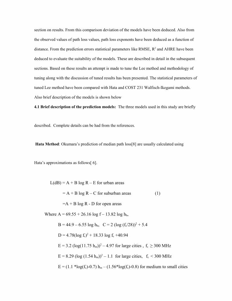
section on results. From this comparison deviation of the models have been deduced. Also from

the observed values of path loss values, path loss exponents have been deduced as a function of

distance. From the prediction errors statistical parameters like RMSE, R2 and AHRE have been

deduced to evaluate the suitability of the models. These are described in detail in the subsequent

sections. Based on these results an attempt is made to tune the Lee method and methodology of

tuning along with the discussion of tuned results has been presented. The statistical parameters of

tuned Lee method have been compared with Hata and COST 231 Walfisch-Ikegami methods.

Also brief description of the models is shown below

4.1 Brief description of the prediction models: The three models used in this study are briefly

described. Complete details can be had from the references.

Hata Method: Okumara’s prediction of median path loss[8] are usually calculated using

Hata’s approximations as follows[ 6].

L(dB) = A + B log R – E for urban areas

= A + B log R – C for suburban areas (1)

=A + B log R - D for open areas

Where A = 69.55 + 26.16 log f – 13.82 log hb,

B = 44.9 – 6.55 log hb, C = 2 (log (fc/28))2 + 5.4

D = 4.78(log fc)2 + 18.33 log fc +40.94

E = 3.2 (log(11.75 hm))2 – 4.97 for large cities , fc ≥ 300 MHz

E = 8.29 (log (1.54 hm))2 – 1.1 for large cities, fc < 300 MHz

E = (1.1 *log(fc)-0.7) hm – (1.56*log(fc)-0.8) for medium to small cities

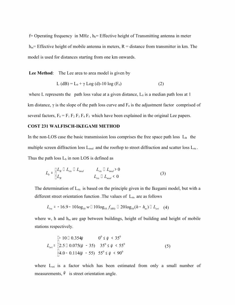
f= Operating frequency in MHz , hb= Effective height of Transmitting antenna in meter hm= Effective height of mobile antenna in meters, R = distance from transmitter in km. The

model is used for distances starting from one km onwards.

Lee Method: The Lee area to area model is given by

L (dB) = L0 + γ Log (d)-10 log (F0) (2)

where L represents the path loss value at a given distance, L0 is a median path loss at 1

km distance, γ is the slope of the path loss curve and F0 is the adjustment factor comprised of

several factors, F0 = F1 F2 F3 F4 F5 which have been explained in the original Lee papers.

COST 231 WALFISCH-IKEGAMI METHOD

In the non-LOS case the basic transmission loss comprises the free space path loss LB the

multiple screen diffraction loss Lmsd and the rooftop to street diffraction and scatter loss Lrts .

Thus the path loss Lb in non LOS is defined as

<+>+++

=00

msdrtsB

msdrtsmsdrtsBb LLL

LLLLLL (3)

The determination of Lrts is based on the principle given in the Ikegami model, but with a

different street orientation function .The values of Lrts are as follows

orimMHzrts LhhfwL +−++−−= )(log20log10log109.16 101010 (4)

where w, h and hm are gap between buildings, height of building and height of mobile

stations respectively.

<≤−−<≤−+

<≤+−=

00

00

00

9055)55(114.00.45535)35(075.05.2

350354.010

ψψψψ

ψψ

oriL (5)

where Lori is a factor which has been estimated from only a small number of

measurements, ψ is street orientation angle.

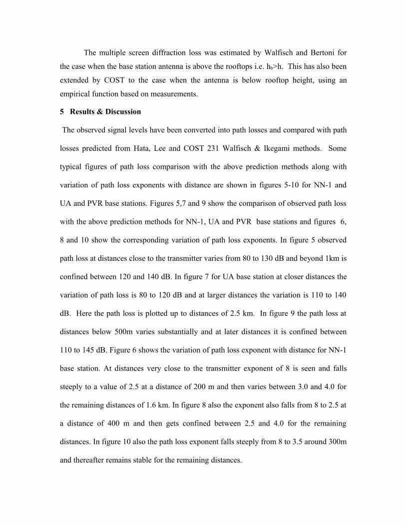
The multiple screen diffraction loss was estimated by Walfisch and Bertoni for

the case when the base station antenna is above the rooftops i.e. hb>h. This has also been

extended by COST to the case when the antenna is below rooftop height, using an

empirical function based on measurements.

5 Results & Discussion

The observed signal levels have been converted into path losses and compared with path

losses predicted from Hata, Lee and COST 231 Walfisch & Ikegami methods. Some

typical figures of path loss comparison with the above prediction methods along with

variation of path loss exponents with distance are shown in figures 5-10 for NN-1 and

UA and PVR base stations. Figures 5,7 and 9 show the comparison of observed path loss

with the above prediction methods for NN-1, UA and PVR base stations and figures 6,

8 and 10 show the corresponding variation of path loss exponents. In figure 5 observed

path loss at distances close to the transmitter varies from 80 to 130 dB and beyond 1km is

confined between 120 and 140 dB. In figure 7 for UA base station at closer distances the

variation of path loss is 80 to 120 dB and at larger distances the variation is 110 to 140

dB. Here the path loss is plotted up to distances of 2.5 km. In figure 9 the path loss at

distances below 500m varies substantially and at later distances it is confined between

110 to 145 dB. Figure 6 shows the variation of path loss exponent with distance for NN-1

base station. At distances very close to the transmitter exponent of 8 is seen and falls

steeply to a value of 2.5 at a distance of 200 m and then varies between 3.0 and 4.0 for

the remaining distances of 1.6 km. In figure 8 also the exponent also falls from 8 to 2.5 at

a distance of 400 m and then gets confined between 2.5 and 4.0 for the remaining

distances. In figure 10 also the path loss exponent falls steeply from 8 to 3.5 around 300m

and thereafter remains stable for the remaining distances.

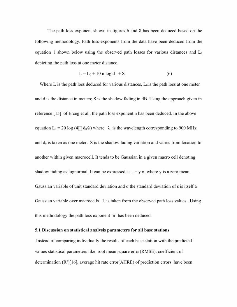
The path loss exponent shown in figures 6 and 8 has been deduced based on the

following methodology. Path loss exponents from the data have been deduced from the

equation 1 shown below using the observed path losses for various distances and L0

depicting the path loss at one meter distance.

L = L0 + 10 n log d + S (6)

Where L is the path loss deduced for various distances, L0 is the path loss at one meter

and d is the distance in meters; S is the shadow fading in dB. Using the approach given in

reference [15] of Erceg et al., the path loss exponent n has been deduced. In the above

equation L0 = 20 log (4∏ d0/λ) where λ is the wavelength corresponding to 900 MHz

and d0 is taken as one meter. S is the shadow fading variation and varies from location to

another within given macrocell. It tends to be Gaussian in a given macro cell denoting

shadow fading as lognormal. It can be expressed as s = y σ, where y is a zero mean

Gaussian variable of unit standard deviation and σ the standard deviation of s is itself a

Gaussian variable over macrocells. L is taken from the observed path loss values. Using

this methodology the path loss exponent ‘n’ has been deduced.

5.1 Discussion on statistical analysis parameters for all base stations

Instead of comparing individually the results of each base station with the predicted

values statistical parameters like root mean square error(RMSE), coefficient of

determination (R2)[16], average hit rate error(AHRE) of prediction errors have been

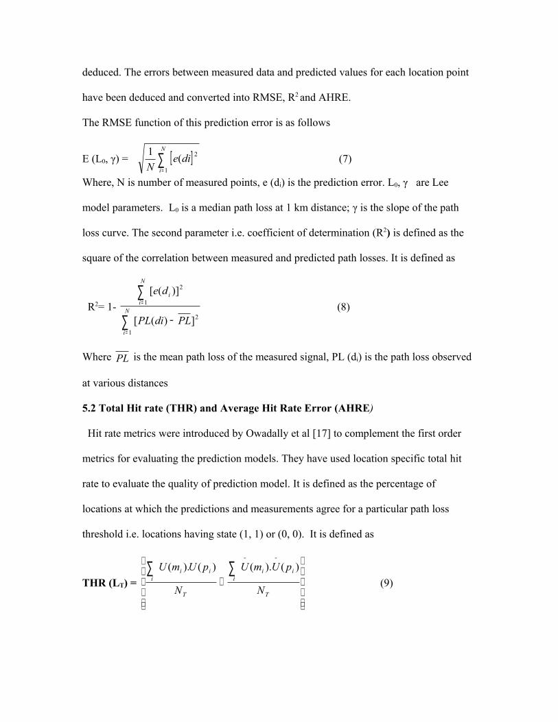
deduced. The errors between measured data and predicted values for each location point

have been deduced and converted into RMSE, R2 and AHRE.

The RMSE function of this prediction error is as follows

E (L0, γ) = [ ]∑=

N

idie

N 1

2(1 (7)

Where, N is number of measured points, e (di) is the prediction error. L0, γ are Lee

model parameters. L0 is a median path loss at 1 km distance; γ is the slope of the path

loss curve. The second parameter i.e. coefficient of determination (R2) is defined as the

square of the correlation between measured and predicted path losses. It is defined as

R2= 1- ∑

∑

=

=

−N

i

N

ii

PLdiPL

de

1

2

1

2

])([

)]([ (8)

Where PL is the mean path loss of the measured signal, PL (di) is the path loss observed

at various distances

5.2 Total Hit rate (THR) and Average Hit Rate Error (AHRE)

Hit rate metrics were introduced by Owadally et al [17] to complement the first order

metrics for evaluating the prediction models. They have used location specific total hit

rate to evaluate the quality of prediction model. It is defined as the percentage of

locations at which the predictions and measurements agree for a particular path loss

threshold i.e. locations having state (1, 1) or (0, 0). It is defined as

THR (LT) =

+∑∑

−−

T

iii

T

iii

N

pUmU

N

pUmU )().()().( (9)

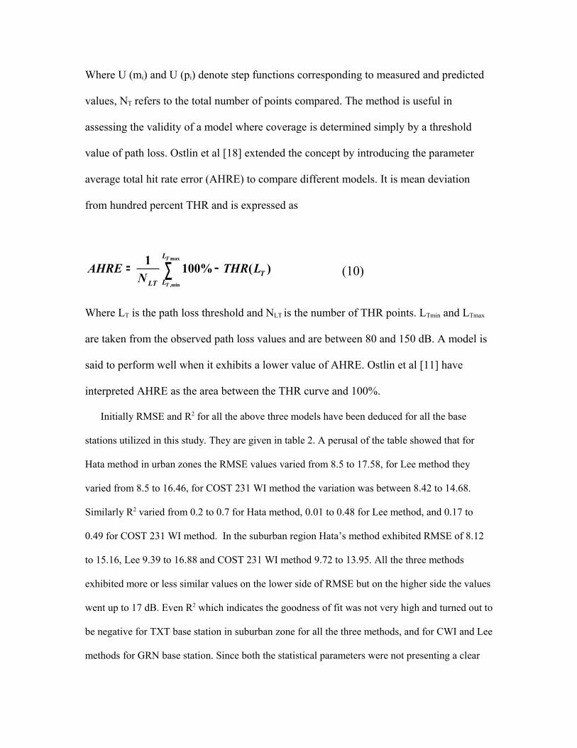
Where U (mi) and U (pi) denote step functions corresponding to measured and predicted

values, NT refers to the total number of points compared. The method is useful in

assessing the validity of a model where coverage is determined simply by a threshold

value of path loss. Ostlin et al [18] extended the concept by introducing the parameter

average total hit rate error (AHRE) to compare different models. It is mean deviation

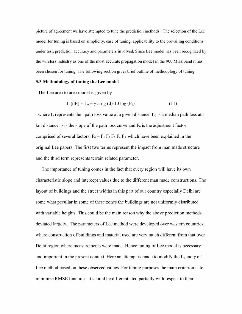
from hundred percent THR and is expressed as

max

,min

1 100% ( )T

T

L

TLLT

AHRE THR LN

= −∑ (10)

Where LT is the path loss threshold and NLT is the number of THR points. LTmin and LTmax

are taken from the observed path loss values and are between 80 and 150 dB. A model is

said to perform well when it exhibits a lower value of AHRE. Ostlin et al [11] have

interpreted AHRE as the area between the THR curve and 100%.

Initially RMSE and R2 for all the above three models have been deduced for all the base

stations utilized in this study. They are given in table 2. A perusal of the table showed that for

Hata method in urban zones the RMSE values varied from 8.5 to 17.58, for Lee method they

varied from 8.5 to 16.46, for COST 231 WI method the variation was between 8.42 to 14.68.

Similarly R2 varied from 0.2 to 0.7 for Hata method, 0.01 to 0.48 for Lee method, and 0.17 to

0.49 for COST 231 WI method. In the suburban region Hata’s method exhibited RMSE of 8.12

to 15.16, Lee 9.39 to 16.88 and COST 231 WI method 9.72 to 13.95. All the three methods

exhibited more or less similar values on the lower side of RMSE but on the higher side the values

went up to 17 dB. Even R2 which indicates the goodness of fit was not very high and turned out to

be negative for TXT base station in suburban zone for all the three methods, and for CWI and Lee

methods for GRN base station. Since both the statistical parameters were not presenting a clear

picture of agreement we have attempted to tune the prediction methods. The selection of the Lee

model for tuning is based on simplicity, ease of tuning, applicability to the prevailing conditions

under test, prediction accuracy and parameters involved. Since Lee model has been recognized by

the wireless industry as one of the most accurate propagation model in the 900 MHz band it has

been chosen for tuning. The following section gives brief outline of methodology of tuning.

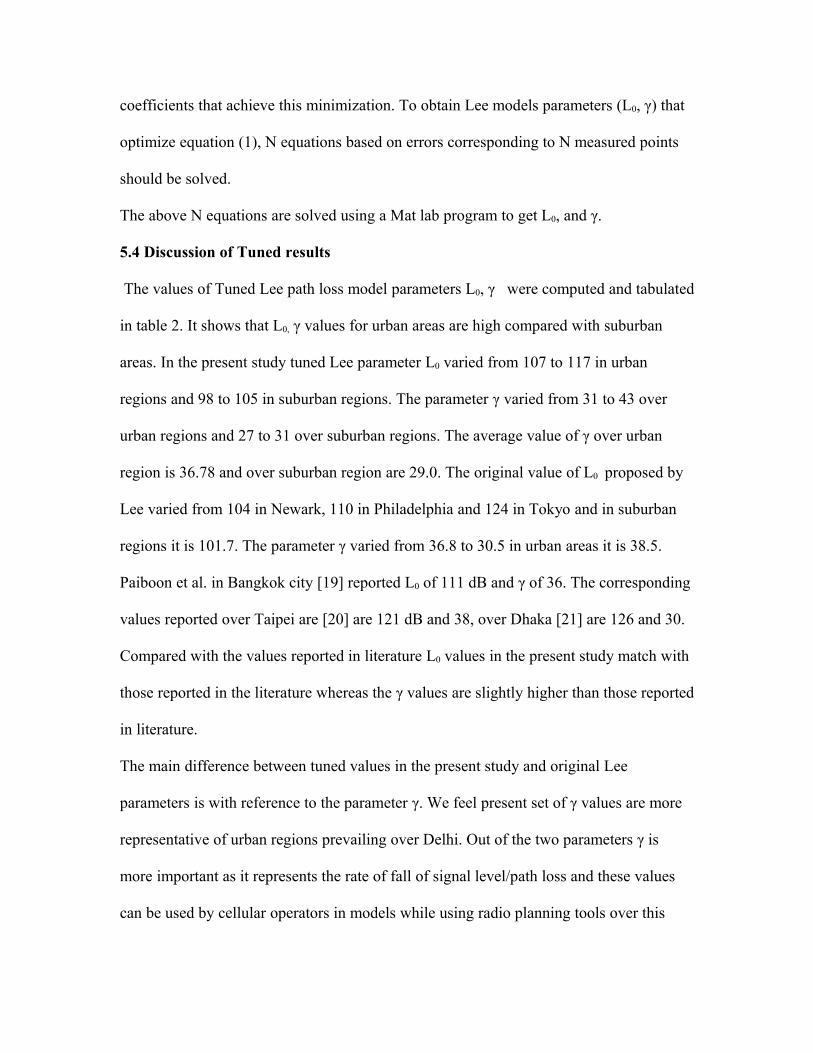
5.3 Methodology of tuning the Lee model

The Lee area to area model is given by

L (dB) = L0 + γ .Log (d)-10 log (F0) (11)

where L represents the path loss value at a given distance, L0 is a median path loss at 1

km distance, γ is the slope of the path loss curve and F0 is the adjustment factor

comprised of several factors, F0 = F1 F2 F3 F4 F5 which have been explained in the

original Lee papers. The first two terms represent the impact from man made structure

and the third term represents terrain related parameter.

The importance of tuning comes in the fact that every region will have its own

characteristic slope and intercept values due to the different man made constructions. The

layout of buildings and the street widths in this part of our country especially Delhi are

some what peculiar in some of these zones the buildings are not uniformly distributed

with variable heights. This could be the main reason why the above prediction methods

deviated largely. The parameters of Lee method were developed over western countries

where construction of buildings and material used are very much different from that over

Delhi region where measurements were made. Hence tuning of Lee model is necessary

and important in the present context. Here an attempt is made to modify the L0 and γ of

Lee method based on these observed values. For tuning purposes the main criterion is to

minimize RMSE function. It should be differentiated partially with respect to their

coefficients that achieve this minimization. To obtain Lee models parameters (L0, γ) that

optimize equation (1), N equations based on errors corresponding to N measured points

should be solved.

The above N equations are solved using a Mat lab program to get L0, and γ.

5.4 Discussion of Tuned results

The values of Tuned Lee path loss model parameters L0, γ were computed and tabulated

in table 2. It shows that L0, γ values for urban areas are high compared with suburban

areas. In the present study tuned Lee parameter L0 varied from 107 to 117 in urban

regions and 98 to 105 in suburban regions. The parameter γ varied from 31 to 43 over

urban regions and 27 to 31 over suburban regions. The average value of γ over urban

region is 36.78 and over suburban region are 29.0. The original value of L0 proposed by

Lee varied from 104 in Newark, 110 in Philadelphia and 124 in Tokyo and in suburban

regions it is 101.7. The parameter γ varied from 36.8 to 30.5 in urban areas it is 38.5.

Paiboon et al. in Bangkok city [19] reported L0 of 111 dB and γ of 36. The corresponding

values reported over Taipei are [20] are 121 dB and 38, over Dhaka [21] are 126 and 30.

Compared with the values reported in literature L0 values in the present study match with

those reported in the literature whereas the γ values are slightly higher than those reported

in literature.

The main difference between tuned values in the present study and original Lee

parameters is with reference to the parameter γ. We feel present set of γ values are more

representative of urban regions prevailing over Delhi. Out of the two parameters γ is

more important as it represents the rate of fall of signal level/path loss and these values

can be used by cellular operators in models while using radio planning tools over this

region and similar regions. Ali [22] over the urban desert regions of Saudi Arabia made

an attempt to tune the values of Lee method on the basis of Tetra measurements in the

400 MHz band. They observed values of γ ranging from 23.47 to 33.8. These values

probably could be due to the different nature of urban environment and frequency used in

this study is 400 MHz. The L0 values reported are 2 to 48. The value 2 appears to be on

the lower side. In this study the standard deviation (RMSE) varied from 3 to 4 in urban

and suburban areas with average RMSE of 3.961 and R2 varied from 0.54 to 0.78. In the

present study after tuning RMSE varied from 5 to 9 and R2 showed variations from 0.29

to 0.79 in urban regions. In suburban regions the corresponding variations are 5.8-10 for

RMSE and 0.29-0.39 for R2. The tuned values of RMSE and R2 are shown in table 1. The

average RMSE for tuned Lee method in urban and suburban zones is found to be 7.69

and 7.68 respectively.

From the table 2, comparison of tuned values of Lee method with other models

showed that the RMSE and R2 values of tuned Lee model performed better than the

traditional models like Hata and COST 231 WI methods. The averaged RMSE value for

all the base stations for the tuned Lee model is 7.69 dB and average RMSE value for

Hata and COST 231 WI models are 11.03, 11.39 respectively for urban regions. Overall

tuned Lee model performed well. In the case of COST 231 WI model the parameters

used are, separation between buildings b=10m, average height of the buildings

hr=6m.The average RMSE value of tuned Lee model is less compared to Hata and COST

231 WI. The R2 value of tuned Lee model is better compared to Hata and COST 231 WI

models. In suburban environments COST 231 WI model over estimated the path loss

values. Hence RMSE and R2 values are not given for TXT tower MPR and GRN base

stations.

Table 3 denotes the AHRE values for all the base stations for the three prediction

methods. In the case of urban region for Hata’s method AHRE varied from 8 to 20.8,

8.16to 19.31 for CWI method, 5 to 15.69 for tuned Lee method. For PVR base station all

the three methods exhibited lowest values ranging from 5.7 for tuned Lee, 8.16 for CWI

and 11.13 for Hata’s method. Highest values were observed for NN 2 base station. For

suburban regions, AHRE varied from 12 to 21.6 for Hata’s method, 15 to 21.2 for CWI

method, 9 to 10 for tuned Lee method. Urban zones exhibited better values than suburban

values. The highlight of the study is the lowest values (improved model performance)

exhibited by tuned Lee method compared with Hata and COST 231 WI for all the base

stations. The average AHRE in urban region for all the base stations are Hata =14.16,

COST 231 WI method = 12.7, tuned Lee method = 10.26. In the case of suburban region

the corresponding values are 16.27, 17.6 & 10.4.These tuned value of Lee method can

also be applied to the similar type of medium urban environment prevailing over various

parts of India and other countries.

6 Conclusions

Signal level measurements were conducted utilizing 7 urban and 4 suburban GSM base

stations in the national capital region of Delhi in the 900 MHz band and the observed

path losses were compared with prediction models like Hata, COST 231 WI and Lee

methods. The comparison of predictions with observed values have been given in terms

of RMSE, R2 and AHRE. Based on the observed path losses the parameters of Lee

method were tuned and new values of parameters L0 and γ were deduced for these

regions. The values of L0 deduced vary from 104 to 117 in urban regions and 98 to 114 in

suburban regions. The parameter γ varied from 14 to 26 over urban regions and 13 to 16

over suburban regions. The statistical metrics of tuned Lee method were seen to

outperform the Hata and COST 231 WI methods significantly.

7 References:1. L.C. Fernandes , A.J. Martins Soares, “ Simplified characterization of the urban propagation environment for path loss calculation, IEEE Antennas and wireless propagation letters, 9,pp 24-27, 20102. Ericsson radio systems AB,TEM STM cellplanner 3.4,User guide, 20013. Digital mobile radio towards future generation systems, COST 231 group final report, COST telecom secretariat, COST@postman.dg13.cec.be4.R.D. Vieira, R.C.D.Paiva , J. Hulkkonen, R. Jarvela, R.F. Iida, M.Saily, F.M.L.Tavares, K. Niemela “GSM evolution importance in re-farming 900 MHz band” in 72nd IEEE international conference on vehicular technology (VTC) 6-9th sept, 2010 fall, pp 1-5., DOI:10.1109/VETECF.2010.5594534.5. D.J.Y. Lee and W.C.Y. Lee, “Enhanced Lee model from rough terrain sampling data aspect” in 72nd IEEE international conf on Vehicular technology (VTC), 6-9th Sep, 2010 fall, pp 1-5, DOI:10.1109/VETECF.2010.5594119 6. M. Hata “Empirical formula for propagation loss in land mobile radio services IEEE Transactions Vehicular Technology, vol.29, pp 317-325, 1980 7. John S.Seybold, “ Introduction to RF Propagation” John Wiley & sons, New Jersey pp 153-154,20058. W.C.Y. Lee “Mobile communication engineering Theory and applications”, 2nd ed., McGraw Hill, New York, pp 59-67, 19939. COST 231, Final report, Digital Mobile Radio: COST 231 View on the evolution Towards 3rd Generation systems, Commission of the European Communities and COST Telecommunications, Brussels, 199910. W C Y Lee, “ Estimation of local average power of a mobile radio signal”, IEEE Trans. Veh. Technology, Vol.VT-34, No.1, 1985

11.W C Y Lee, “Mobile communication design fundamentals”, Howard W. Sams and Co., 1986

12. International Telecommunication union, “Field strength measurements along a route

with geographical coordinate registrations, ITU-R recommendation SM.1708, April 2005

13. European Conference of Postal and Telecommunications Administrations, “ERC

Report,77, Field strength measurements along a route:, ERC REc.08(00), January 2000

14. International Telecommunication Union, “Generalized method for monitoring

broadcasting signals and for the analysis of field strength variation. Application to

ground wave propagation in MF band” ITU documents 3J/26-E and 3K/22-E, May2008

15. V. Erceg, S.Y. Tjandra, S.R. Parkoff, Ajay Gupta, Boris Kulic, A.A. Julius and Renee Bianchi, “An empirically based path loss model for wireless channels in suburbanenvironments”, IEEE J Selected areas in Communications, vol.17, no.7, pp 1205-1211, 1999

16. R.E. Walpole and R.H. Myers, “Probability and statistics for Engineers and scientists, 3rdedition, Macmillan, New York, pp 353, 1985

17. A.S. Owadallly, E. Montiel and S.R. Saunders S. R. “A comparison of the accuracy of propagation models using hit rate analysis”, in 54th IEEE conf on Vehicular Technology (VTC), vol.4, pp 1979-1983, 2001 fall

18. E. Ostlin, H.Suzuki and H.J. Zepernick, “Evaluation of the propagation model recommendation ITU-R P.1546 for mobile services in rural Australia IEEE Trans Vehicular Technology, vol.57,no.1, pp 38-51,2008

19. S. Phaiboon, P. Phokharatkul and S. Somkuarnpanit, Propagation-Path losses characterization for 800 MHz cellular communications in Bangkok”, in Proceeding of the IEEE Region 10 Conference(TENCON 99),vol. 2,pp 1209-1211,15-17september 1999 20. Chien-Chung Wang and Jhin-Fang Huang, Propagation path loss characterization for an 870 MHz cellular CDMA system in Taipei city”, in Proc. IEEE international symposium on Microwave, Antenna, Propagation and EMC Technologies for Wireless communications, pp 790-793, 16-17 Aug 2007

21. A.B.M. Siddique Hossain and Md. Ramjan Ali, “ Propagation path losses characterization for 900 MHz cellular communications in Dhaka city” in proc. of 9th

Asia-Pacific conference, vol.1, 21-24 Sept,2003.

22. Faihan D.Alotaibi and Ali A.A, “ Tetra Outdoor Large-Scale Received Signal Prediction Model in Riyadh City-Saudi Arabia” in proc. of IEEE Wireless and Microwave technology Conference (WAMICON) pp 1-5, 4-5 Dec,2006

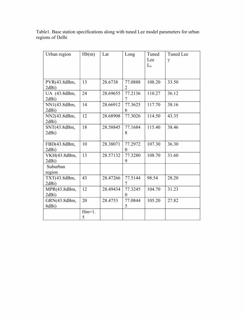
Table1. Base station specifications along with tuned Lee model parameters for urban regions of Delhi

Urban region Hb(m) Lat Long Tuned LeeL0

Tuned Leeγ

PVR(43.8dBm,2dBi)

13 28.6738 77.08882

108.20 33.50

UA (43.8dBm,2dBi)

24 28.69655 77.21367

110.27 36.12

NN1(43.8dBm,2dBi)

14 28.66912 77.36256

117.70 38.16

NN2(43.8dBm,2dBi)

12 28.68908 77.3026 114.50 43.35

SNT(43.8dBm,2dBi)

18 28.58845 77.16848

115.40 38.46

FBD(43.8dBm,2dBi)

10 28.38071 77.29720

107.30 36.30

VKH(43.8dBm,2dBi)

13 28.57132 77.32809

108.70 31.60

Suburban regionTXT(43.8dBm,2dBi)

43 28.47266 77.51447

98.54 28.20

MPR(43.8dBm,2dBi)

12 28.49434 77.32450

104.70 31.23

GRN(43.8dBm,8dBi)

20 28.4753 77.08445

105.20 27.82

Hm=1.5

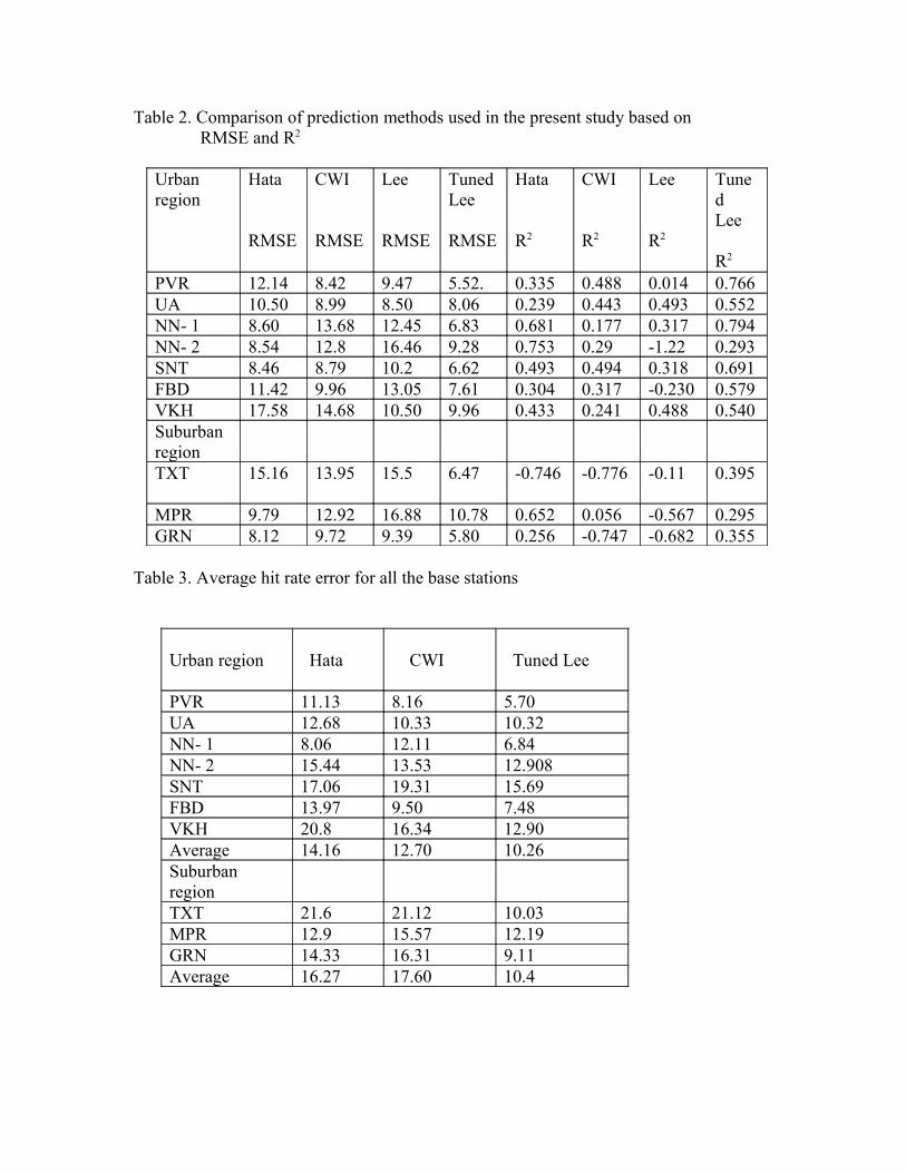
Table 2. Comparison of prediction methods used in the present study based on RMSE and R2

Urban region

Hata

RMSE

CWI

RMSE

Lee

RMSE

Tuned Lee

RMSE

Hata

R2

CWI

R2

Lee

R2

Tuned Lee

R2

PVR 12.14 8.42 9.47 5.52. 0.335 0.488 0.014 0.766UA 10.50 8.99 8.50 8.06 0.239 0.443 0.493 0.552NN- 1 8.60 13.68 12.45 6.83 0.681 0.177 0.317 0.794NN- 2 8.54 12.8 16.46 9.28 0.753 0.29 -1.22 0.293SNT 8.46 8.79 10.2 6.62 0.493 0.494 0.318 0.691FBD 11.42 9.96 13.05 7.61 0.304 0.317 -0.230 0.579VKH 17.58 14.68 10.50 9.96 0.433 0.241 0.488 0.540Suburban regionTXT 15.16 13.95 15.5 6.47 -0.746 -0.776 -0.11 0.395

MPR 9.79 12.92 16.88 10.78 0.652 0.056 -0.567 0.295GRN 8.12 9.72 9.39 5.80 0.256 -0.747 -0.682 0.355

Table 3. Average hit rate error for all the base stations

Urban region Hata

CWI

Tuned Lee

PVR 11.13 8.16 5.70UA 12.68 10.33 10.32NN- 1 8.06 12.11 6.84NN- 2 15.44 13.53 12.908SNT 17.06 19.31 15.69FBD 13.97 9.50 7.48VKH 20.8 16.34 12.90Average 14.16 12.70 10.26Suburban regionTXT 21.6 21.12 10.03MPR 12.9 15.57 12.19GRN 14.33 16.31 9.11Average 16.27 17.60 10.4

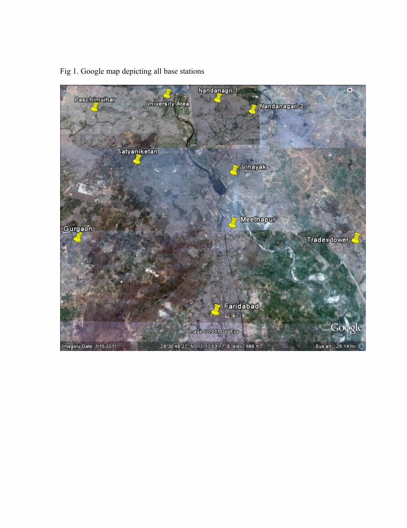
Fig 1. Google map depicting all base stations

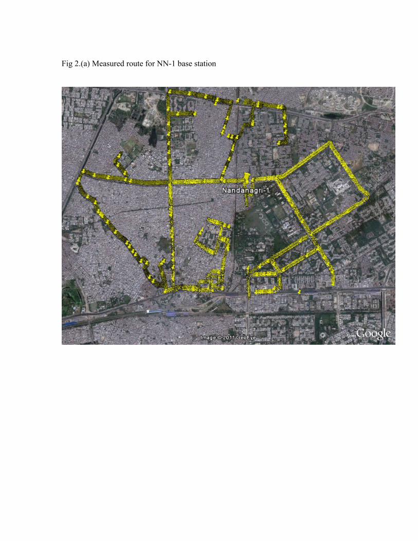
Fig 2.(a) Measured route for NN-1 base station

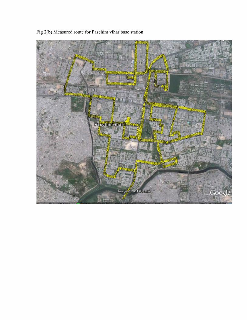
Fig 2(b) Measured route for Paschim vihar base station

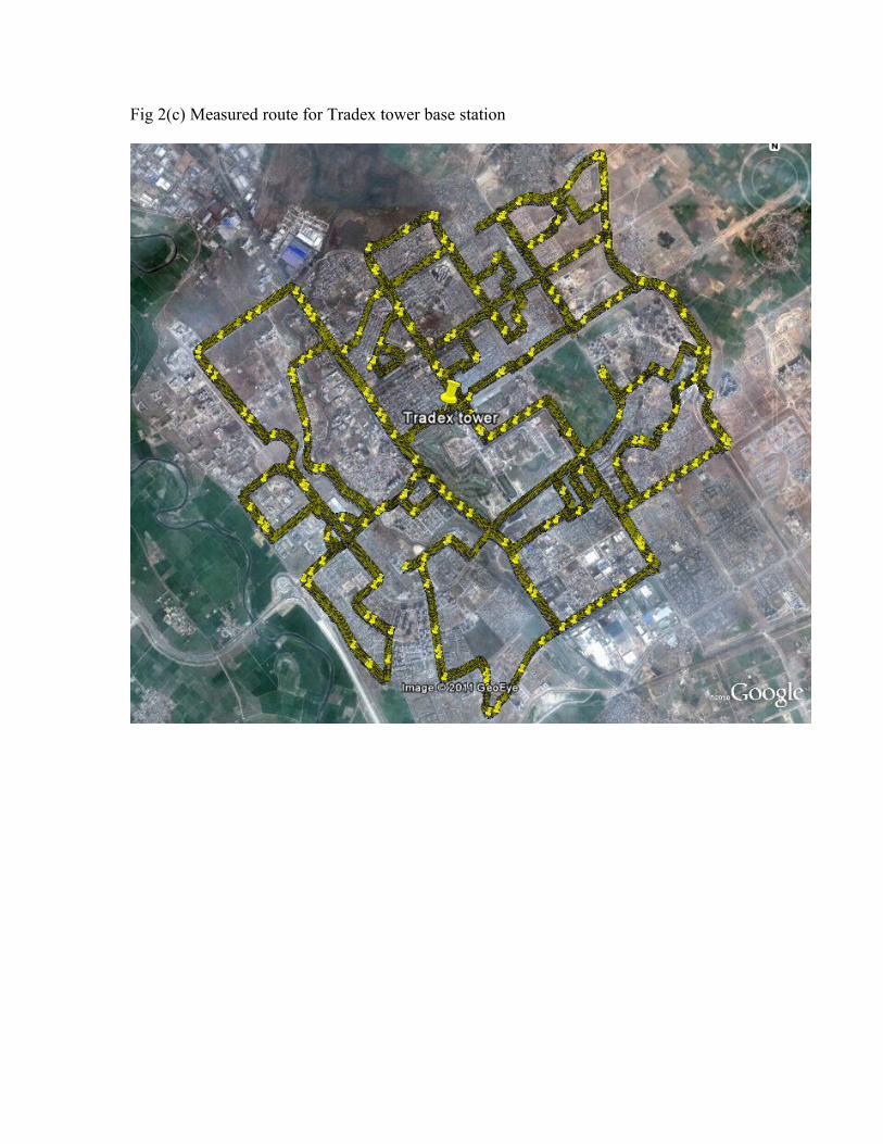
Fig 2(c) Measured route for Tradex tower base station

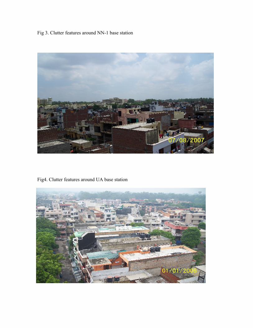
Fig 3. Clutter features around NN-1 base station

Fig4. Clutter features around UA base station

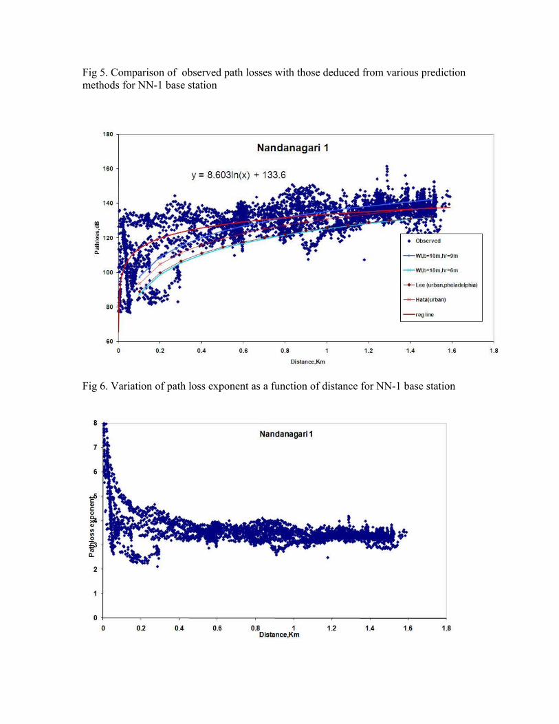
Fig 5. Comparison of observed path losses with those deduced from various prediction methods for NN-1 base station

Fig 6. Variation of path loss exponent as a function of distance for NN-1 base station

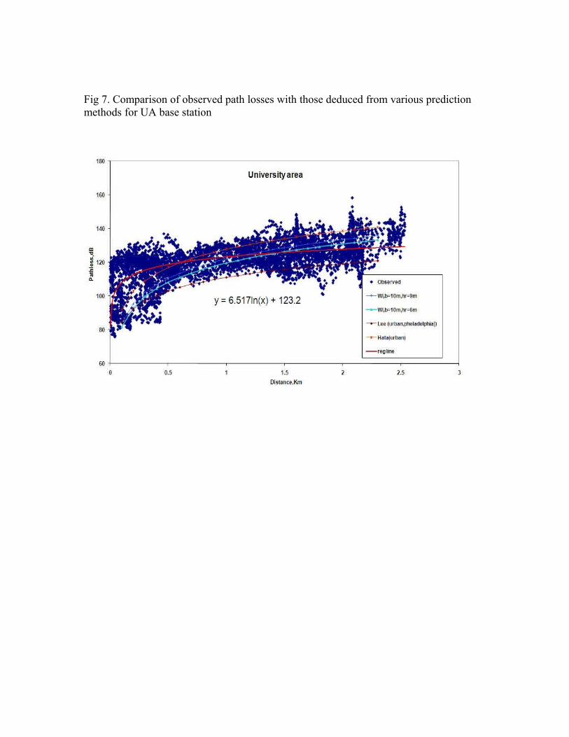
Fig 7. Comparison of observed path losses with those deduced from various prediction methods for UA base station

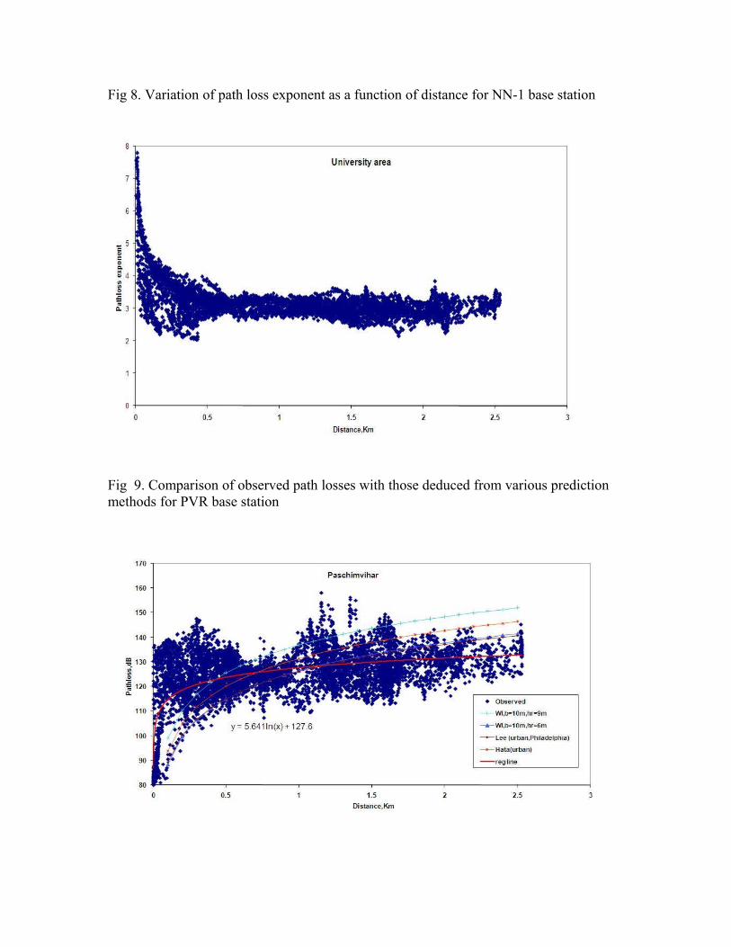
Fig 8. Variation of path loss exponent as a function of distance for NN-1 base station

Fig 9. Comparison of observed path losses with those deduced from various prediction methods for PVR base station

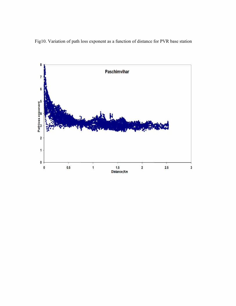
Fig10. Variation of path loss exponent as a function of distance for PVR base station