Evaluation of an Expansion of the Electricity Transmission ...
71
Evaluation of an Expansion of the Electricity Transmission System in Mexico Glenn P. Jenkins Queen’s University, Kingston, Canada. Eastern Mediterranean University, North Cyprus. Henry B.F. Lim Independent Economic Consultant and Gangadhar P. Shukla Development Discussion Paper Number: 1999-5 Abstract In the past, most evaluations of the electric utility investments have been based on the assumptions that the suppliers of electricity would provide the quantity of energy demanded at an acceptable level of reliability. The question addressed in most of the investment appraisals has been: “is this investment the least cost way to supply the electricity demanded?” In real life the situation is usually very different in most developing countries. Shortages, outages and deterred demand have been the rule, rather than the exception. Often the existing generation, transmission and distribution system are far from being the least cost method of supplying power. As a consequence, major investments are required to improve the existing capacity of electricity systems as well as to provide some expansion. In such a situation both the financial and economic analyses become more challenging. We need to isolate both benefits and costs of incremental investments that are part of an overall integrated system, where existing assets rather than new assets dominate the system’s operations. This study of a major rehabilitation program by Commission Federal de Electricidad (CFE) of Mexico (Mexico Public Electric Utility) presents a practical method of analysis for this type of projects along several fronts. Such an integrated analysis is much more than a set of procedures for estimating the expected net present values or rates of return of the project. An investment appraisal carried out in this fashion becomes an analytical tool for redesigning the project in ways that increase the likelihood of its sustainability and the probability of achieving its objectives. Previously Published: Development Discussion Paper No. 688, Harvard Institute for International Development, Harvard University, March 1999. JEL code(s): D61, H43, L95 Key words: Mexico, electricity, rehabilitation, investment, generation, electricity, transmission, cost-benefit analysis.
Transcript of Evaluation of an Expansion of the Electricity Transmission ...

Evaluation of an Expansion of the Electricity Transmission System in Mexico
Glenn P. Jenkins Queen’s University, Kingston, Canada.
Eastern Mediterranean University, North Cyprus. Henry B.F. Lim
Independent Economic Consultant
and Gangadhar P. Shukla
Development Discussion Paper Number: 1999-5 Abstract In the past, most evaluations of the electric utility investments have been based on the assumptions that the suppliers of electricity would provide the quantity of energy demanded at an acceptable level of reliability. The question addressed in most of the investment appraisals has been: “is this investment the least cost way to supply the electricity demanded?” In real life the situation is usually very different in most developing countries. Shortages, outages and deterred demand have been the rule, rather than the exception. Often the existing generation, transmission and distribution system are far from being the least cost method of supplying power. As a consequence, major investments are required to improve the existing capacity of electricity systems as well as to provide some expansion. In such a situation both the financial and economic analyses become more challenging. We need to isolate both benefits and costs of incremental investments that are part of an overall integrated system, where existing assets rather than new assets dominate the system’s operations. This study of a major rehabilitation program by Commission Federal de Electricidad (CFE) of Mexico (Mexico Public Electric Utility) presents a practical method of analysis for this type of projects along several fronts. Such an integrated analysis is much more than a set of procedures for estimating the expected net present values or rates of return of the project. An investment appraisal carried out in this fashion becomes an analytical tool for redesigning the project in ways that increase the likelihood of its sustainability and the probability of achieving its objectives. Previously Published: Development Discussion Paper No. 688, Harvard Institute for International Development, Harvard University, March 1999. JEL code(s): D61, H43, L95 Key words: Mexico, electricity, rehabilitation, investment, generation, electricity, transmission, cost-benefit analysis.

Harvard Institute forInternational Development
HARVARD UNIVERSITY
Evaluation of an Expansion of theElectricity Transmission System
in Mexico
Glenn P. Jenkins, Henry B.F. Lim,and Gangadhar P. Shukla
Development Discussion Paper No. 688March 1999
© Copyright 1999 Glenn P. Jenkins, Henry B.F. Lim, Gangadhar P. Shukla,and President and Fellows of Harvard College
Development Discussion Papers

HIID Development Discussion Paper no. 688
Evaluation of an Expansion of the Electricity Transmission System in Mexico
Glenn P. Jenkins, Henry B.F. Lim, and Gangadhar P. Shukla*
Abstract
In the past, most evaluations of the electric utility investments have been based on the assumptions that the suppliers ofelectricity would provide the quantity of energy demanded at an acceptable level of reliability. The question addressed in mostof the investment appraisals has been: “is this investment the least cost way to supply the electricity demanded?”
In real life the situation is usually very different in most developing countries. Shortages, outages and deterred demandhave been the rule, rather than the exception. Often the existing generation, transmission and distribution system are far frombeing the least cost method of supplying power. As a consequence, major investments are required to improve the existingcapacity of electricity systems as well as to provide some expansion. In such a situation both the financial and economic analysesbecome more challenging. We need to isolate both benefits and costs of incremental investments that are part of an overallintegrated system, where existing assets rather than new assets dominate the system’s operations.
This study of a major rehabilitation program by Comision Federal de Electricidad (CFE) of Mexico (Mexico PublicElectric Utility) presents a practical method of analysis for this type of projects along several fronts. First, the analysis is donein an integrated fashion where the financial, economic, distributive, and risk aspects of the project are examined together on aconsistent basis. Second, the value of each of the components of the supply improvement, i.e reduction in shortages, outages,transmission losses, is considered separately and then combined in the overall appraisal. Third, the risks imposed on theseinvestments from such macro-economic variables as changes in the real exchange rate and the rate of inflation are modeled,based on real world data, and combined with the risks inherent in the project inputs, such as fuel and investment costs to makean assessment of the overall risks associated with the undertaking of these investments.
Such an integrated analysis is much more than a set of procedures for estimating the expected net present values orrates of return of the project. An investment appraisal carried out in this fashion becomes an analytical tool for redesigning theproject in ways that increase the likelihood of its sustainability and the probability of achieving its objectives.
Keywords: Mexico, electricity, rehabilitation, investment, generation, transmission, appraisal
JEL Codes: D61, H43, L94
Glenn P. Jenkins is an Institute Fellow at the Harvard Institute for International Development, Henry Lim is aResearch Fellow at the International Tax Program, Harvard Law School, and G.P. Shukla is a DevelopmentAssociate at the Harvard Institute for International Development, Harvard University.
*This study has benefited greatly from the collaboration and assistance of a number of people. Alfred Thieme has been aconstant source of advice and encouragement. Luis E. Gutierrez and Nisan Ceran spent a great deal of time to provide us withessential information from the World Bank archives and to provide us with a better understanding of the electricity sector inMexico. The analytical and computational efforts of Eloi D. Traore were essential for the completion of the analysis. Thecollaboration of our colleagues, George Kuo, Alberto Barreix, Mario Marchesini, Migara Jayawardena, Harmawan RubinoSugana, and Raghavendra Narain was always helpful, and greatly appreciated. Any errors and omissions that remain are ourresponsibility. Comments on this paper may be addressed to: [email protected]
HIID Development Discussion Paper no. 688
Evaluation of an Expansion of the Electricity Transmission System in Mexico
Glenn P. Jenkins, Henry B.F. Lim, and Gangadhar P. Shukla
I. OVERVIEW
In the early 1980s, Mexico went through a period of economic recession characterized byhigh rates of inflation and a large external debt. Mexico responded by implementingmacroeconomic reforms which were aimed at opening up the economy to foreign competition,limiting the role of the state in the productive sectors, fostering the development of nontraditional exports and rescheduling the foreign debt.
In the mid-1980s the reforms were successful in stabilizing the economy. Thestabilization program that started in December 1987 reduced substantially the level of inflation.Inflation rate dropped from a high 159.2%, in 1987, to 19.2% in 1989. That drop in inflationresulted from the reduction in the size of the government deficit, which was achieved byincreasing the price of goods and services supplied by government enterprises, and by adopting arestrictive fiscal and monetary policy.
Along with macroeconomic reforms, several measures in different sectors of the economywere implemented to reduce the public deficit and to raise economic efficiency. In the energysector for example, fuel prices were increased in real terms to correct the distortions in resourceallocation, public sector procurements for the sector were opened to foreign competition, andrates-schedules were allowed to increase in line with inflation and the operating costs of thesector.
In the electricity sector, the government restricted the investments by Comission Federalde Electricidad (CFE) to a minimum. In the 1970’s CFE investment averaged 13% of total publicinvestment. That share dropped in the 1980s to remain fairly constant at 10% from 1982 to 1989while the annual amounts declined from year to year in terms of constant 1989 prices. From afigure of US$ 2 billion in 1982, total investment in the electricity sector was US$1.4 billion in1983, 1984, and 1985. A further decline to US$ 1.15 billion occurred in 1986 and 1987.
The reduction of public investment in the sector forced CFE to postpone its least-costinvestment program, which included the construction and maintenance of generating plants, andtransmission and distribution equipment. Consequently, the electricity sector faced severaltechnical problems; such as reduction of reserves in generating plants, increase in energy losses,and reduction in the supply and efficiency of thermal-electric generating plants.
With favorable economic conditions after mid-1980, public investment was resumed andCFE planned to expand its productive capabilities and achieve its objectives by implementing along-term investment program which would take into account economic issues as well as
2
financial restrictions. The total direct investment of this program, US$ 35 billion for the period1989-1998.
The lending program of the World Bank, in accordance with the country assistancestrategy, aimed at lending slightly more than US 2 billion per year to Mexico. Thus, the WorldBank would serve as Mexico’s “lead bank” and play a major catalytic role in securing externalsources of financing for: (a) continued adjustment (agriculture, public enterprises, fiscalreform/deregulation, public sector enterprises); (b) increasing sector investment (time-slicelending for irrigation, power, transport, water); and (c) expanded lending in human resources,poverty alleviation and the environment1. It is in that context of country assistance strategy thatthe World Bank authorized a loan to assist in financing the construction of hydro generatingplants in May 1989. In the same year, the bank prepared a lending operation to finance the 1991-92 time-slice investment program for CFE in transmission and distribution facilities, and inreconditioning thermal-electric plants.
The Electricity Sector in Mexico
Mexico has two public electric utilities that operate in the power sector. The first utility,CFE (Comission Federal de Electricidad) is in operation since 1937. It generates, transmits anddistributes electricity to the whole country. The second company, CLFC (The Compania de Luzy Fuerza del Centro), a former private utility now wholly owned by CFE, is in charge of thedistribution in the area of Mexico city and the vicinity.
The installed capacity of CFE at the end of 1988 included 23,921 MW in generationplants, 56,000 km of high voltage transmission lines (400 Kv, 230 Kv and 115 Kv), 255,000 kmof distribution lines, and 16,500 MVA of distribution transformers. Although most of the countryis interconnected through high voltage transmission lines, the full exchange of power plantreserves is not possible because of the limitations in the interconnection of different regions.
CFE estimated that, for the decade 1988-98, sales including export would grow at 6.6%.Should demand grow at a faster rate and the rate of investment in the power sector remainunchanged, the reliability of supply would deteriorate leading to a shortage situation.Consequently, as part of the ten-year investment program, CFE prepared four specialsubprograms that would be implemented over a five-year period to address specific problems inthe areas of generation, transmission, distribution and rehabilitation of thermal plants.
CFE planned to add 17,626 MW in new power generation plants during the period 1989-98. Besides that generation program, CFE undertook three subprograms in generation,transmission, and distribution during the period 1990-94. The subprogram in generation wouldrenovate the thermoelectric power plants to improve thermal efficiency and availability at CFE’smain plants. The subprogram “Transmission” expanded and improved installations rated 400 kvto 115 kv. Finally, the subprogram “Distribution” aimed at connecting new customers, and atimproving the reliability of the service of major activities in Distribution.
1 Mexico Country Strategy Paper, World Bank, 1993.

3
Transmission Project Objective and Benefits
The primary objective of the project under study was to expand and improve transmissioninstallations rated 400 kv to 115 kv. The benefits come from increased consumption because ofnew customers, from transformer and lines loss reduction and from outages reduction.
In the financial analysis, the benefits from increased consumption are valued using thevalue of the transmission service, which is the share of the weighted average tariff less the fueland operating costs attributed to transmission. The financial savings from loss reduction2 arevalued using fuel, operating, and generation capacity costs. The financial revenues fromreduction of outages are simply valued as the product of the resulting increased consumption andthe weighted average tariff.
The economic benefits from increased consumption are calculated using the willingnessto pay approach. The economic benefits of loss reduction are calculated using the conversionfactors for fuel, operating costs, and generation capacity costs. The economic benefits from thereduction of outages are valued at the costs of electricity to the end users. A survey on the costsof outages can be carried out for each group of customers to determine the average opportunitycost of the energy when outages occur.
Results of the Financial, Economic, Distributive, and Risk Analyses.
This study evaluates the Transmission Subprogram by using an integrated financial-economic-distributive approach. The economic analysis assesses the value to the economy of theproject's output and inputs. It adjusts the financial values for any distortions such as taxes,subsidies, or foreign exchange premium, which cause financial prices to differ from true resourcevalues.
The results of the base case indicate that if this project could be implementedsuccessfully, the net present values from the total investment perspective and from the economicpoint of view would respectively be 1,619 and 3,894 billion pesos or US$ 527 and US$ 1,268million (in 1990 prices).
The distributive analysis shows that consumers benefit most from this project. They gain3,155 billion pesos or US$ 1,027 million (1990 prices). Labor benefits by 86 billion Pesos (US$28 million) while the government gains 652 billion Pesos (US $ 212 million).
The results of the risk analysis show that the net present values from the total investmentperspective and from the economic point of view are 1,957 and 3,842 billion pesos respectively.
2 An alternative would be to value loss reductions using the tariff since the energy saved because of the reduction oflosses is now available for sale. This study makes an assumption that in the long run, savings in fuel, operating costsand capacity building are realized. Therefore, it is appropriate to use these savings rather than the tariff to calculatethe benefits from loss reduction.

4
II. PROJECT DESCRIPTION
The transmission system at CFE covers most of the country’s territory in Mexico. As of1989, the system comprised approximately 24,000 km of high voltage lines (69 to 400 KV), and66,000 MVA of capacity installed in substations. Seven regional divisions were in charge of thedesign, construction, maintenance and operation of the transmission system. Five of these regionswere interconnected while the regions of Peninsular and Baja California were isolated from thenational grid. All these regions are part of this project.
The reduction of public investment in the electricity sector in the 1980s forced CFE topostpone its least-cost investment. With better economic conditions at the end of that decade,public investment resumed and CFE, faced with many technical problems, planned to upgrade itsproductive capabilities in the three areas of the system.
The purpose of this special subprogram in the area of transmission is to connect newcustomers to the grid, to reduce transmission losses, and to improve the reliability of the system.
A. Project Components
This project includes the following components:
• Installation of new transformers with a capacity of 10,400 MVA in existing or newsubstations, and 1,020 circuit breakers.
• Construction of a total of 700 high voltage feeders and transmission lines with a totallength of 7,500 km.
Transmission lines
The evaluation of a transmission project requires the analyst to identify the different typesof transmission lines. There exist three types of transmission lines: (1) lines that link generationplants to the national grid; (2) lines that connect two isolated systems; and (3) lines thatreinforce and expand the existing system. The objective of this project is to reinforce and expandthe existing grid system. The current project does not include the connection of the two isolatedsystems, Peninsular and Baja California, to the national grid even though part of the investmentwill be made in those regions. This project deals only with the third type of the transmission linesdescribed above. Table 1 summarizes the various transmission lines that are part of this project.

5
Table 1: Total Transmission Lines (in Km) by Level of Voltage
Area 400 KV 230 KV 138 KV 115 KV 69 KV TotalOriental 238 940 1674 2852Occidental 360 782 372 28 1542Nordeste 49 390 439Norte 216 123 339Noreste 887 86 973Peninsular 380 372 752BajaCalifornia
138 303 146 587
Total (Km) 1485 2505 86 3234 174 7484
Transformers
The objective of installing new transformers and circuit breakers is either to reduce theload of existing ones or to take on new demand. When the load of transformers exceeds thetransformers’ capacity, the losses increase substantially and the reliability of the electrical systemdecreases. In that situation, it is necessary to replace existing transformers by new ones withgreater capacity or install new transformers to reduce the load of existing transformers.
As the project consists of replacing old transformers or installing new ones to supply theexisting demand, the incremental benefits of this project would include the reduction oftransformers losses and the improvement in reliability. The measurement of transformers lossesis given by a chart provided by the manufacturer of the transformer. The losses in kilowatts arethen converted into energy losses. The value of the incremental benefits from the reduction oftransformer losses is the product of the energy losses (in kwh) and the cost savings per Kwh. Thisper unit savings per Kwh is measured by the marginal cost of generating and transmitting powerto the substation where the transformers are installed.
The replacement of old transformers or the installation of new ones generates two typesof revenues. The revenues from the sales of electricity to new customers and the savings due tothe reduction of losses.

6
Table 2 shows the total capacity installed by the project by level of voltage for eachregion.
Table 2: Transformers’ capacity installed with project (MVA)
Area 400 Kv 230 Kv 161 Kv 115 Kv 69 Kv Total(MVA)
Oriental 1130 988 923.4 3041.4Occidental 1375 1831 134 268.8 80 3688.8Nordeste 430 320 750Norte 500 594 270 1364
Noreste 363 86 363Peninsular 400 248.8 648.8B.California 312 170 60 542Total 3005 4918 134 2201 140 10398
B. Alternatives Considered
This project is part of the least cost investment program of CFE in its transmissionsystem. CFE has several planning models for optimization of the transmission system associatedwith schemes for expanding the generation. The other investment mixes, which are not describedhere, were analyzed by the models to come up with the investment program which has the lowestpresent value of costs and meets the capacity requirements overtime.
C. Project Cost and Financing
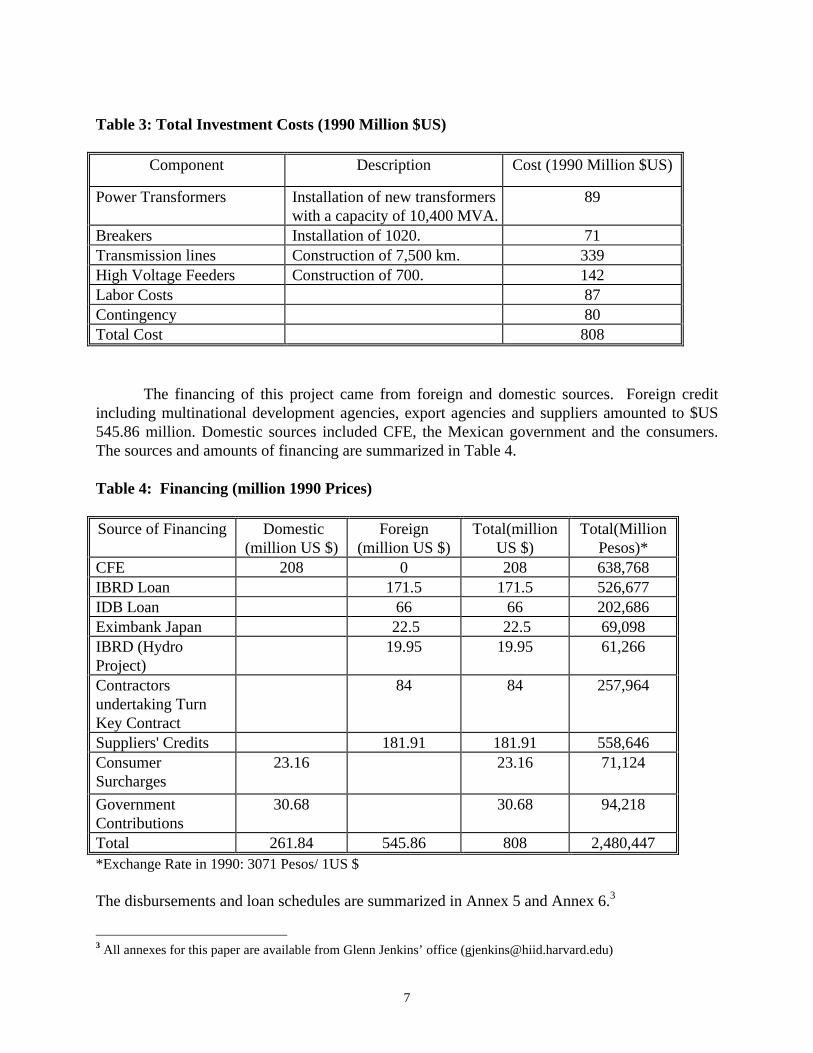
The estimated total cost of the project, including the costs of equipment, materials, labor,engineering, and supervision is $US 808 million in 1990 prices of which $US 545.86 million(67.6%) is in foreign currency and $US 262.14 million (32.4%) is in local currency. Totalinvestment costs including equipment, labor cost, and contingencies for cost overruns aresummarized in Table 3:
7
Table 3: Total Investment Costs (1990 Million $US)
Component Description Cost (1990 Million $US)
Power Transformers Installation of new transformerswith a capacity of 10,400 MVA.
89
Breakers Installation of 1020. 71Transmission lines Construction of 7,500 km. 339High Voltage Feeders Construction of 700. 142Labor Costs 87Contingency 80Total Cost 808
The financing of this project came from foreign and domestic sources. Foreign creditincluding multinational development agencies, export agencies and suppliers amounted to $US545.86 million. Domestic sources included CFE, the Mexican government and the consumers.The sources and amounts of financing are summarized in Table 4.
Table 4: Financing (million 1990 Prices)
Source of Financing Domestic(million US $)
Foreign(million US $)
Total(millionUS $)
Total(MillionPesos)*
CFE 208 0 208 638,768IBRD Loan 171.5 171.5 526,677IDB Loan 66 66 202,686Eximbank Japan 22.5 22.5 69,098IBRD (HydroProject)
19.95 19.95 61,266
Contractorsundertaking TurnKey Contract
84 84 257,964
Suppliers' Credits 181.91 181.91 558,646ConsumerSurcharges
23.16 23.16 71,124
GovernmentContributions
30.68 30.68 94,218
Total 261.84 545.86 808 2,480,447*Exchange Rate in 1990: 3071 Pesos/ 1US $
The disbursements and loan schedules are summarized in Annex 5 and Annex 6.3
3 All annexes for this paper are available from Glenn Jenkins’ office ([email protected])
8
D. A Public Sector or Private Sector Project?
Even if the institutional framework in the area of electricity transmission were developedin Mexico to allow for the private provision of this service, a private enterprise would not havean incentive to undertake this investment, which is mainly an upgrade of the existing system.Also, private provision of the transmission of electricity alone is not sufficient for the project tobe done in the private sector as the benefits of this project are mainly arising from the savings ingeneration of electricity. Indeed, 50 % of the financial benefits come from the savings ingeneration costs and these benefits accrue directly to CFE, the principal owner of the generatingplants. To attract the private sector, part of these savings would have to be credited to the privateowner of the transmission system.
The question remains whether a multilateral institution, such as the World Bank, shouldbe financing this project or should CFE obtain its financing from private financial institutions?This question cannot be answered without further information on the costs and risks facing bothCFE and the private financial institutions if the funds were obtained from such sources. Giventhe considerable real exchange rate risk associated with foreign borrowing to produce what isessentially a non-traded good, the sources of funds from a multilateral organization with theguarantee of the national government might be an efficient way to manage the associated risks ofsuch a project. In this case, however, the question of the private sector undertaking thisinvestment is not considered, as it is an enhancement of the existing CFE system, and CFE is astate-owned enterprise.
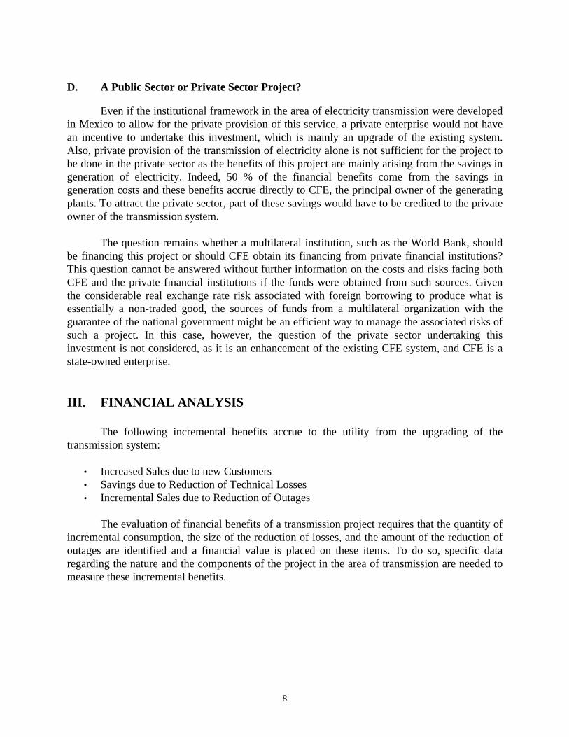
III. FINANCIAL ANALYSIS
The following incremental benefits accrue to the utility from the upgrading of thetransmission system:
• Increased Sales due to new Customers• Savings due to Reduction of Technical Losses• Incremental Sales due to Reduction of Outages
The evaluation of financial benefits of a transmission project requires that the quantity ofincremental consumption, the size of the reduction of losses, and the amount of the reduction ofoutages are identified and a financial value is placed on these items. To do so, specific dataregarding the nature and the components of the project in the area of transmission are needed tomeasure these incremental benefits.
9
Service of a Transmission Line
The service of a transmission line depends on the net energy delivered by the line to thedistribution system or to the customers directly connected to that transmission line. That netenergy is the difference between the energy received from generation and the sum of the line andtransformer losses.
Tariff Share of the Transmission Service
The challenge in valuing the service of a transmission line for a regulated integratedelectrical utility arises from the absence of a tariff for the services of transmission alone.
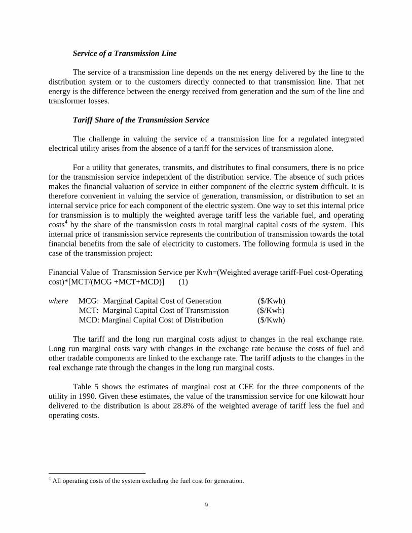
For a utility that generates, transmits, and distributes to final consumers, there is no pricefor the transmission service independent of the distribution service. The absence of such pricesmakes the financial valuation of service in either component of the electric system difficult. It istherefore convenient in valuing the service of generation, transmission, or distribution to set aninternal service price for each component of the electric system. One way to set this internal pricefor transmission is to multiply the weighted average tariff less the variable fuel, and operatingcosts4 by the share of the transmission costs in total marginal capital costs of the system. Thisinternal price of transmission service represents the contribution of transmission towards the totalfinancial benefits from the sale of electricity to customers. The following formula is used in thecase of the transmission project:
Financial Value of Transmission Service per Kwh=(Weighted average tariff-Fuel cost-Operatingcost)*[MCT/(MCG +MCT+MCD)] (1)
where MCG: Marginal Capital Cost of Generation ($/Kwh) MCT: Marginal Capital Cost of Transmission ($/Kwh) MCD: Marginal Capital Cost of Distribution ($/Kwh)
The tariff and the long run marginal costs adjust to changes in the real exchange rate.Long run marginal costs vary with changes in the exchange rate because the costs of fuel andother tradable components are linked to the exchange rate. The tariff adjusts to the changes in thereal exchange rate through the changes in the long run marginal costs.
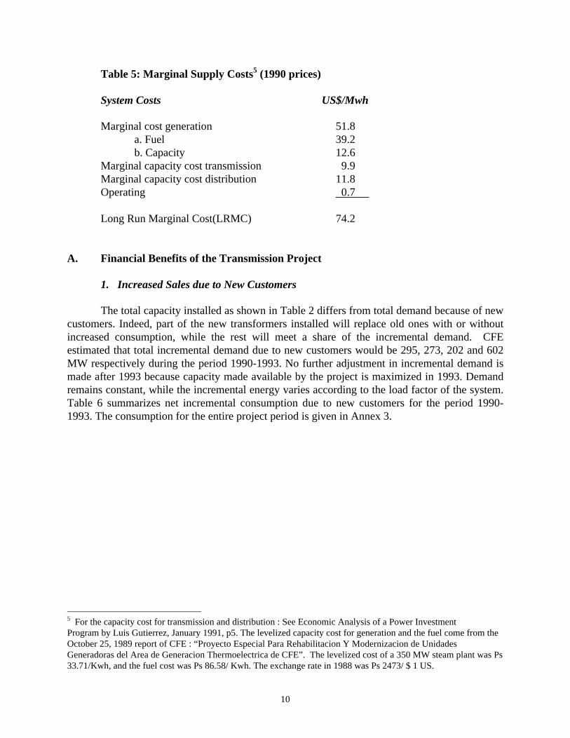
Table 5 shows the estimates of marginal cost at CFE for the three components of theutility in 1990. Given these estimates, the value of the transmission service for one kilowatt hourdelivered to the distribution is about 28.8% of the weighted average of tariff less the fuel andoperating costs.
4 All operating costs of the system excluding the fuel cost for generation.
10
Table 5: Marginal Supply Costs5 (1990 prices)
System Costs US$/Mwh
Marginal cost generation 51.8a. Fuel 39.2b. Capacity 12.6
Marginal capacity cost transmission 9.9Marginal capacity cost distribution 11.8Operating 0.7
Long Run Marginal Cost(LRMC) 74.2
A. Financial Benefits of the Transmission Project
1. Increased Sales due to New Customers
The total capacity installed as shown in Table 2 differs from total demand because of newcustomers. Indeed, part of the new transformers installed will replace old ones with or withoutincreased consumption, while the rest will meet a share of the incremental demand. CFEestimated that total incremental demand due to new customers would be 295, 273, 202 and 602MW respectively during the period 1990-1993. No further adjustment in incremental demand ismade after 1993 because capacity made available by the project is maximized in 1993. Demandremains constant, while the incremental energy varies according to the load factor of the system.Table 6 summarizes net incremental consumption due to new customers for the period 1990-1993. The consumption for the entire project period is given in Annex 3.
5 For the capacity cost for transmission and distribution : See Economic Analysis of a Power InvestmentProgram by Luis Gutierrez, January 1991, p5. The levelized capacity cost for generation and the fuel come from theOctober 25, 1989 report of CFE : “Proyecto Especial Para Rehabilitacion Y Modernizacion de UnidadesGeneradoras del Area de Generacion Thermoelectrica de CFE”. The levelized cost of a 350 MW steam plant was Ps33.71/Kwh, and the fuel cost was Ps 86.58/ Kwh. The exchange rate in 1988 was Ps 2473/ $ 1 US.

11
Table 6: Incremental Consumption For The Period 1990-1993
1990 1991 1992 1993
Net IncrementalDemand (MW)
295 273 202 602
Cumulative netdemand (MW)
295 568 770 1372
Load Factor6 54.61% 52.96% 51.28% 49.37%
Net energysold7 (Gwh)
1411 2635 3459 5933
Using the value of service defined in equation (1) above, Table 7 shows the calculation ofthe sales revenues for the period 1990-1993. The present value of sales revenues fromincremental consumption due to new customers amounts to 2,230 billion pesos or US$ 726million (1990 prices) from the whole project. This represents 46% of the project’s financialrevenues.
6 The load factor is derived from the projections of both energy and system capacity of the whole electric system.Load Factor= Projected Energy Demanded/(8760*Projected System Capacity )7 Energy Sold(Gwh)= 8.76* Incremental Demand (Mw)*Load Factor

12
Table 7: Measurement of Revenues from Incremental Electricity Sales to New Customers for Period 1990-1993 (Nominal Prices)
1990 1991 1992 1993
Net energy sold8
(Gwh)1411 2635 3459 5933
Nominal tariff 9
(million pesos/Mwh) (a)
0.114 0.153 0.205 0.276
Fuel Cost10
(million Pesos/Mwh) (b)
0.1203 0.1384 0.1591 0.1830
Operating Cost11
(MillionPesos/Mwh) (c)
0.0021 0.0024 0.0028 0.0032
Value ofTransmissionService12
(million pesos/Mwh) (d)
(0.0086) (0.0037) 0.0043 0.0165
Revenues(million Pesos)
(12,119) (9,634.2) 14,727.7 97,609.8
Revenues13
(million US $)(3.95) (2.82) 3.88 23.17
To obtain the transmission sales revenues of 97,609 million pesos or US$ 23.17 millionfor the year 1993 as shown in table 7, we make the following calculations. In 1993, the total salesto new customers amounted to 5933 Gwh. The nominal price of electricity was 0.276 millionpesos per Mwh while the fuel cost was 0.183 million pesos per Mwh. Hence, the difference
8 Energy Sold(Gwh)= 8.76* Incremental Demand (Mw)*Load Factor.9 Nominal tariff= Weighted Average Nominal Gross of Tax Tariff.10 The fuel cost in 1990 was US$ 39.2/Mwh. To obtain the value in nominal pesos, the fuel cost is expressed in realpesos and then multiplied by the price index in subsequent years.11 The operating cost in 1990 was US$ 0.7 /Mwh. The method used for the fuel is also applicable here.12 Value of transmission service= [a-(b+c)/(1-0.15)]*0.2877. The sum (b+c) is divided by (1-0.15) to take intoaccount the additional fuel and operating costs induced by 15 % of system losses.13 The projected nominal exchange rates from 1990 to 1993 are 3071, 3412, 3791,and 4213 pesos/1 US$respectively.

13
between the electricity price and the sum of fuel and operating costs adjusted for energy losses14
is 0.0572 million pesos per Mwh. This difference multiplied by the share of the transmissioncapital cost to the total system capital cost, which is 28.77%, gives the value of the transmissionservice as 0.0165 million pesos per Mwh. This value of the transmission service is multiplied bythe quantity of electricity sold to new customers, 5933 Gwh, to obtain the financial salesrevenues of 97,609 million pesos derived from new customers.
2. Reduction of Technical losses
Technical losses in the area of transmission refer essentially to losses in transmissionlines and transformers, and losses due to failure of transmission equipment. The incrementalenergy saved is the difference of total losses in two situations: “with” and “without” project. Thecalculation of these losses can be simple or complex depending upon the nature of the project.When the project involves the integration of transmission lines and transformers into aninterconnected network, the assessment of incremental benefits is more difficult.15
Transmission losses
There are three types of transmission losses: line losses, transformer losses and losses ofsynchronous condensers. Each of these losses can be evaluated easily for a single componentsuch as one transmission line, or one transformer. The difficulty arises when that singlecomponent is part of a dynamic network. In this case, all components of the system interact andthe calculation of transmission losses becomes complex.
The transmission-line losses vary with the loads at both ends of the line, the length of theline, the power factor, and the level of voltage16. A transmission network, however, consists ofmany lines, transformers, condensers and the power flows through the system following theroutes of least resistance. The operating conditions affect all parts of equipment of an electricsystem. When electric equipment such as transformers and transmission lines are overloaded, thelosses increase.
In the case of a network, the valuation of losses is not straightforward. A system flowmodel is usually constructed to simulate the power flow and losses of the system. In this project,the results from two scenarios of a load flow model “with project” and “without project” are used 14 The energy losses amount to 15% of generation.15 Max J. Steinberg and Theodore H. Smith, Economy Loading of Power Plants and Electric Systems.16 For a three-phase transmission line that links two stations, the line losses in KW are given by
TL = R (kw)2 + R (kvar)2
1000 (kv)2 1000 (kv)2
where,R= line resistance per wire in ohmskvar = total three-phase transmitted reactive kilovolt-amperes.kw = total three-phase transmitted energy.kv = line voltage, in kilovolts.TL = total three-phase line losses, in kilowatts

14
to calculate the reduction of losses due to the project. The output of the model of load flowsincludes both incremental consumption and loss reduction. The following data in Table 8 showsonly the loss reduction estimated by CFE’s system flow model in the “with” and “without”project scenario for the period 1990-93. After 1993, the losses17 expressed in megawatts in agiven year are the product of losses in the previous year and the ratio of total demand in thatgiven year and total demand in the previous year.
Table 8: Technical losses for the period 1990-93
Technical losses 1990 1991 1992 1993
With Project (MW) 276 280 303 349
Without Project (MW) 445 471 546 658
Reduction of Losses(MW)
169 191 243 309
Load Factor 54.61% 52.96% 51.28% 49.37%
With Project (GWH) 841 810 831 898
Without Project (GWH) 1356 1361 1497 1692
Reduction of losses(GWH)
515 551 666 794
17 To convert the losses expressed in megawatts into gigawatt-hours the following equation is used:
Losses (Gwh) = L*8.76*[0.8*Lf^2+0.2*Lf]where L: Losses in MW Lf: Load factor

15
Table 9 shows the calculation of the benefits from loss reduction for the period 1990-1993.
Table 9: Measurement of Savings from Loss Reduction for Period 1990-1993 (NominalMillion Pesos)
1990 1991 1992 1993
Reduction inlosses18 (Gwh)(a)
515 551 666 794
Fuel Cost19 perMwh (b)
0.1203 0.1384 0.1591 0.1830
OperatingCost20 per Mwh (c)
0.0021 0.0024 0.0028 0.0032
MarginalGenerationCapacityCost21
per Mwh(d)
0.039 0.044 0.051 0.059
Savings perMwh of lossreduction22 (e)
0.1614 0.1848 0.2129 0.2452
Total Savingsdue to Lossreduction23
83,121 101,825 141,791 194,689
The financial benefits from savings in transmission losses are created because a reductionin these losses allows the system to generate a smaller quantity of electricity and still deliver thesame amount of energy to its customers. Hence, the savings are estimated here by multiplying thesum of the fuel, and marginal generation capacity costs, and operating costs by the quantity of thereduced losses.
18 The reduction in losses are calculated in Table 8.19 See footnote 10.20 See footnote 11.21 The generation capacity cost in 1990 was US$ 12.6/Mwh. To obtain the value in nominal pesos, the capacity costis expressed in real pesos and then multiplied by the domestic price index in subsequent years.22 Savings per unit of loss reduction = (b)+(c)+(d)23 Total savings = (a)*(e) *1000

16
In the short run, the savings in generation capacity costs may not be realized. However, inthe long run, the approach used to evaluate the savings due to loss reduction takes into accountthe degree to which generation capacity costs are saved through a reduction in transmissionlosses. For this project, the present value of the savings in variable generation costs due to lossreduction in substations and transmission lines amounts to 2,413 billion pesos (1990 prices),which is about 50% of the total financial benefits of the project.
3. Increased Sales due to Reduction of Outages
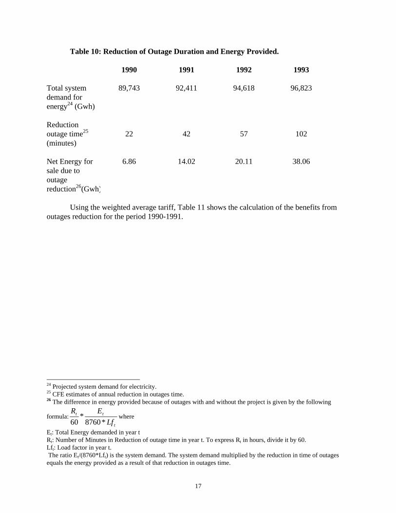
Table 10 provides the estimated decline in the total duration of the interruptions andoutages. CFE has estimated, based on computer models, a total annual reduction of 102 minutesin outages duration by the year 1993 due to the implementation of this project. In 1992, thereduction in outages duration is the product of the time in 1993, which is 102 minutes, and theratio of the incremental demand in 1992 and 1993 respectively. The same procedure is used tocalculate the reduction in outages time for the years 1991 and 1990. After 1993, the reduction intotal outages time remains at 102 minutes.
The incremental consumption due to outage reduction is distinct from the incrementaldemand calculated earlier. The incremental consumption due to outage reduction relates toexisting customers who suffer from outages. Since the duration of outages in this case affects thewhole electric system, the value of reduced outages is therefore the product of the incrementalenergy sold because of outage reduction and the weighted average tariffs of different groups ofconsumers.
17
Table 10: Reduction of Outage Duration and Energy Provided.
1990 1991 1992 1993
Total systemdemand forenergy24 (Gwh)
89,743 92,411 94,618 96,823
Reductionoutage time25
(minutes)22 42 57 102
Net Energy forsale due tooutagereduction26(Gwh)
6.86 14.02 20.11 38.06
Using the weighted average tariff, Table 11 shows the calculation of the benefits fromoutages reduction for the period 1990-1991.
24 Projected system demand for electricity.25 CFE estimates of annual reduction in outages time.26 The difference in energy provided because of outages with and without the project is given by the following
formula:t
tt
Lf
ER
*8760*
60where
Et: Total Energy demanded in year tRt: Number of Minutes in Reduction of outage time in year t. To express Rt in hours, divide it by 60.Lft: Load factor in year t. The ratio Et/(8760*Lft) is the system demand. The system demand multiplied by the reduction in time of outagesequals the energy provided as a result of that reduction in outages time.

18
Table 11: Revenues from Outages Reduction For Period 1990-1993 (Nominal Prices)
1990 1991 1992 1993Sales fromoutagesreduction27
(Gwh)6.86 14.02 20.11 38.06
Nominal tariff28
(million pesos/Mwh)
0.114 0.153 0.205 0.276
Revenues fromoutagesreduction29
(million Pesos)
782 2,145 4,123 10,504
The present value of revenues due to reduction of total outages time for the entire projectamounts to 216 billion pesos30 or US$ 70 million (1990 prices) for the whole project, or fourpercent of the project’s financial benefits.
B. Methodology of Financial Analysis
The first step in financial analysis consists of making assumptions about variables such astariff, inflation, interest during construction, income tax and sales taxes, project economic life,and working capital. The second step consists of carrying out the analysis in both nominal andreal prices from the total investment and equity owner’s perspectives. The analysis in bothnominal and real prices sheds light on the impact of inflation on the project. Inflation has bothdirect and indirect effects on the results of the analysis. The indirect impacts, also known as thetax impacts, are relevant when the equity owner is subject to corporate income tax. The directeffects of inflation take place through changes in accounts receivable, changes in accountspayable and changes in cash balances.
1. Assumptions
A. Tariff Policy
Although the level of tariff is very important for the financial sustainability of a regulatedelectric utility, this project illustrates how measurement of financial savings from loss reductionis as important as the end user tariff. Because the fuel cost alone is about 53% of the long runmarginal cost of the system, the reduction of losses due to the transmission project will have a
27 See footnote 18.28 Weighted Average Nominal Gross of Tax Tariff.29 Calculated as the product of sales due to outages reduction and the nominal weighted average gross of tax tariff.30 Stream of revenues from outage reduction for entire life of project discounted at financial discount rate of 7.17%.
19
significant effect on the financial results of this project. Indeed, the results of the financialanalysis confirm that 50% of total benefits come from loss reduction. The importance of the fuelcost savings of generation created by this project does not mean that the analysis of tariff shouldbe neglected.
The tariff used in this study is consistent with the new tariff policy agreement signed in1989 between CFE and the government. There are two major issues confronting electricity tariffin Mexico. First, electricity rates have been subsidized by the government since the 1970s, andsecond, the tariff structure does not reflect the costs of supplying electricity to each customerclass. Electricity rates fell in real terms by about 37% between 1980 and 1983 because of thehigh rate of inflation and a lag in the adjustment of nominal tariff. Despite the sharp increases innominal terms from 1984 to 1988, the rates did not reach the 1980 level.
Facing both issues of subsidies and high inflation, the government and CFE signed a newFinancial Rehabilitation Agreement (FRA) on August 31, 1989. One measure adopted in theFRA was for CFE to update the tariff study in order to establish a program of rate increases inreal terms in accordance with macroeconomic conditions. Under that scheme, most governmentsubsidies except those to low-income residential and rural users would be eliminated by 1991,and average electricity rate would reach the Long Run Marginal Cost (LRMC) level by 1996. Inthis study, we assume that all customers tariff reach their LRMC level by the year 1996.
After eliminating the government subsidies, another condition has to be met to achievethe LRMC target by the year 1996: nominal electricity rates have to fully adjust to inflation.Thus, this study considers that nominal electricity rates will be adjusted to inflation with a lagperiod of three months to account for institutional and other constraints in setting electricityprices.
B. Inflation
Inflation in Mexico in the 1960s and up until 1972 remained low within the range of1.5% to 5%. The OPEC oil price hike led to a double-digit inflation in 1973 and the followingyears. Between 1973 and 1982, inflation fluctuated between 12% and 28% range. Between 1983and 1988 inflation rates were high and unstable reaching a high of 114% in 1988. Given suchinstability, it is difficult to predict long-term inflation rates. However, since the government aimsat reducing the level of inflation to that of Mexico’s main trading partners, a 15% inflation ratewas assumed in the base case analysis of this study. The possible fluctuations in the rate ofinflation are considered in the sensitivity and risk analysis.
C. Interest During Construction and Capital Cost
There are different ways to consider interest during construction (IDC) in a financialanalysis. First, if interest has been paid during the period of construction then it enters theanalysis as a cash outflow when the project is examined from the equity owner’s point of view.Second, if no interest on the loan has been paid out during the construction period, which is the
20
case in this project, then interest during construction is accrued and added to the total investmentafter completion of the project for depreciation purposes.
D. Income Tax and VAT on Electricity.
CFE as a state-owned electric utility is not subject to corporate income tax. The valueadded tax on electricity is 15%.
E. Project’s Economic Life
The project was to be completed in four years starting in 1990. CFE estimated aneconomic life of 30 years for the main equipment of the transmission subprogram.
F. Accounts Receivable, Accounts Payable, Cash Balances
Accounts payable are set at one and a half months of fuel and operating expenses. Also,cash balances that are held as working capital are assumed to be three months of these expenses.
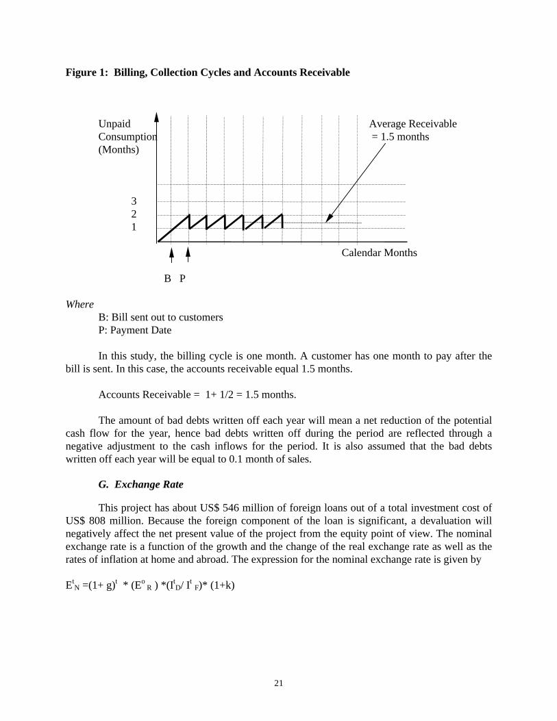
The level of accounts receivable is a function of the billing and collection cycles, and theuncollectibles receivable (bad debt). For a utility that sells essential services to customers andbills them on a regular basis, the nature of its billing and collection cycles can have substantialimpact on the firm’s revenues. For instance, a power company may bill the customer everymonth after reading the meter, and allow the customer to pay within one month after the bill issent. This will result in a billing cycle of one month, and a collection cycle of 1 month. Therelationship between the length of billing cycle, the collection period and the level of accountsreceivable expressed in months of sales can be written as31:
Accounts Receivable (in months of sales)= Billing cycle + Average Collection Cycle/2
31 In this study, accounts receivable is equal to the unpaid sales rather than unpaid bills. Unpaid consumption isalways greater than the unpaid bills.
21
Figure 1: Billing, Collection Cycles and Accounts Receivable
Unpaid Average ReceivableConsumption = 1.5 months(Months)
321
Calendar Months
B P
WhereB: Bill sent out to customersP: Payment Date
In this study, the billing cycle is one month. A customer has one month to pay after thebill is sent. In this case, the accounts receivable equal 1.5 months.
Accounts Receivable = 1+ 1/2 = 1.5 months.
The amount of bad debts written off each year will mean a net reduction of the potentialcash flow for the year, hence bad debts written off during the period are reflected through anegative adjustment to the cash inflows for the period. It is also assumed that the bad debtswritten off each year will be equal to 0.1 month of sales.
G. Exchange Rate
This project has about US$ 546 million of foreign loans out of a total investment cost ofUS$ 808 million. Because the foreign component of the loan is significant, a devaluation willnegatively affect the net present value of the project from the equity point of view. The nominalexchange rate is a function of the growth and the change of the real exchange rate as well as therates of inflation at home and abroad. The expression for the nominal exchange rate is given by
EtN =(1+ g)t * (Eo
R ) *(ItD/ It F)* (1+k)

22
WhereEt
N = Nominal Exchange rate at period t.g = Rate of real devaluationEo
R = Real Exchange rate as of Period 0.It
D = Domestic price Index at Period t.It F = Foreign Price Index at Period t.k = Deviation of the Rate of real devaluation from the trend in the movement of thereal exchange rate.
The rate of real devaluation assumed over time in the base case is zero.
C. Points of View and Discount Rates
The financial analysis in both nominal and real prices were conducted from the equity andthe total investment points of view. From the total investment point of view, the viability of theproject is analyzed irrespective of financing while from the equity’s viewpoint the debt and itsrepayments are included in the cash flows.
The real return on equity recommended in the Financial Rehabilitation Agreement is 7%.The Agreement has also suggested a funding mix of 47.4 % from external borrowing, 5.4% fromgovernment and 47.2% from internal sources. The real returns on these sources of financing wererespectively 7.17 %, 8.6% and 7%. The funding mix and the real rates of returns yield a realweighted average cost of capital (WACC) of 7.17%, which is used as real discount rate in thetotal investment perspective.
The financial net present value from both equity and total investment viewpoints areestimated by discounting the annual projected stream of cash flows by their respective discountrate. Annexes 2 to 9 show the tables used to construct the net cash flow statement. These tablesinclude the loans schedule, electricity tariff, investment cost, operating and maintenanceexpenses and working capital. After conducting the analysis in current pesos, the nominal cashflows are deflated by the price index to obtain the real (1990 pesos) cash flows.
D. Results of Financial Analysis
The financial benefits of this project come from increased consumption due to newcustomers, loss reduction, and increased consumption due to outages time reduction. Increasedconsumption due to new customers represents 46% of total financial benefits, while lossreduction and outages time reduction amount respectively to 50% and 4% of total financialbenefits. The 50% share of total benefits from loss reduction signals that special care should betaken in the estimation of these losses. The sensitivity analysis will show the net impact of thelosses on the net present value of this project. Table 12 summarizes the present values of eachtype of benefit.

23
Table 12: Present Value of Benefits and Cost Savings for Entire Life of the ProjectPresent Value(Million of 1990Pesos)
Present Value(Million of 1990US$ )
% Total Benefits
Benefits fromIncreased sales dueto new customers
2,229,760 726 46%
Benefits from lossReduction
2,413,118 786 50%
Benefits fromoutages reduction
216,502 70 4%
Total 4,859,380 100%
Table 13 shows the results of the financial analysis. The net present values from the totalinvestment point of view and from the equity point of view are respectively 1,619 and 2,003billion of pesos or US$ 527 million and US$ 652 million.
Table 13: Summary of Financial Cash Flow AnalysisReal Discount
RateReal NPV
(Million Pesos)Real NPV
(Million US $)IRR
TotalInvestmentPoint of View
7.17% 1,619,513 527 12%
Equity Point OfView (CFE) 7% 2,003,064 652 21%
Equity Point OfView (withoutgov. grants)
7% 1,853,251 603 18%
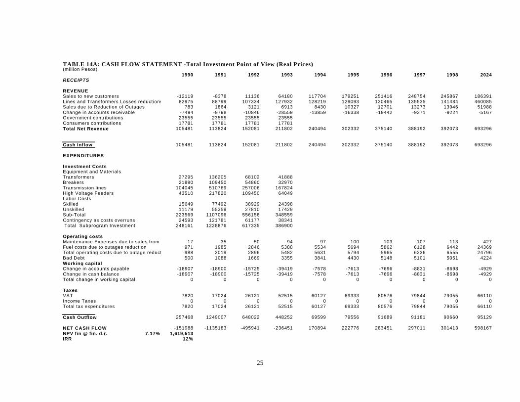
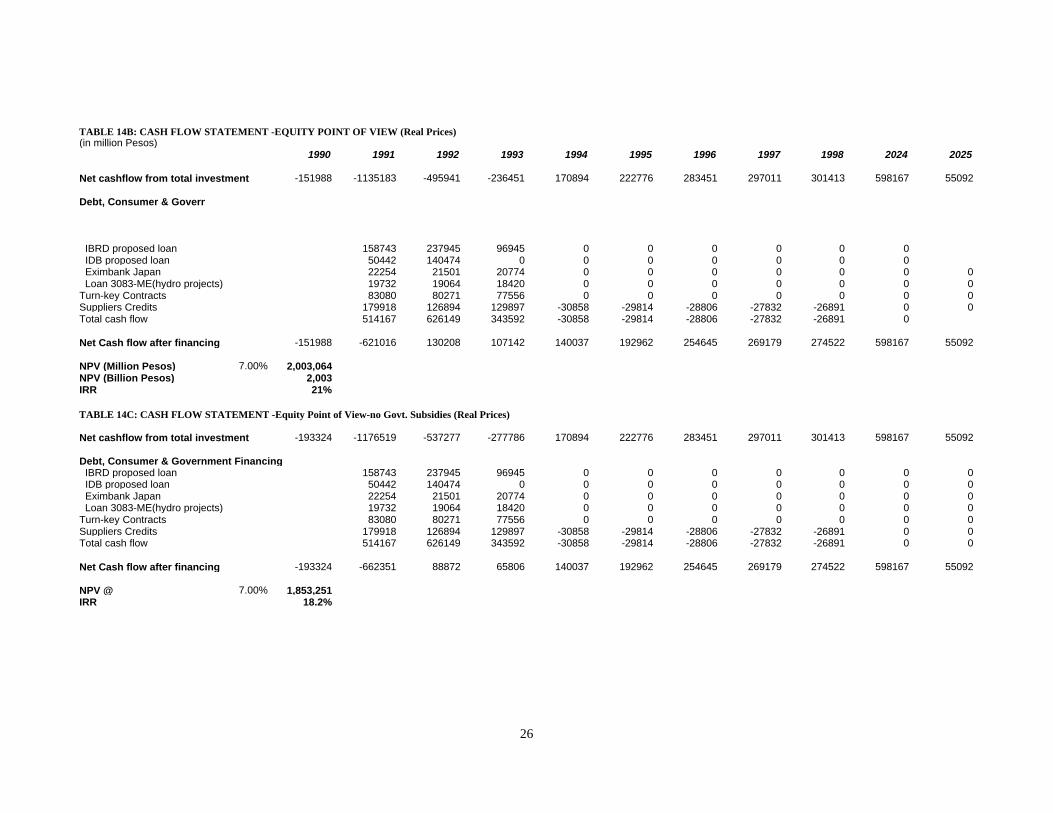
Tables 14a,14b, and 14c show the results of the projected real cash flow statement fromthe total investment, the equity owner’s, and the equity owner’s excluding government grants32
perspectives respectively.
32 The government will grant US$ 30.68 million to finance this project. This grant is included in the Total Investmentperspective as a cash inflow. The NPV from the equity owner’s perspective remains positive even if this amount ofUS$ 30.68 million is not accounted for as a cash inflow.

25
TABLE 14A: CASH FLOW STATEMENT -Total Investment Point of View (Real Prices)(million Pesos)
1990 1991 1992 1993 1994 1995 1996 1997 1998 2024RECEIPTS
REVENUESales to new customers -12119 -8378 11136 64180 117704 179251 251416 248754 245867 186391Lines and Transformers Losses reductions 82975 88799 107334 127932 128219 129093 130465 135535 141484 460085Sales due to Reduction of Outages 783 1864 3121 6913 8430 10327 12701 13273 13946 51988Change in accounts receivable -7494 -9798 -10846 -28559 -13859 -16338 -19442 -9371 -9224 -5167Government contributions 23555 23555 23555 23555Consumers contributions 17781 17781 17781 17781Total Net Revenue 105481 113824 152081 211802 240494 302332 375140 388192 392073 693296
Cash Inflow 105481 113824 152081 211802 240494 302332 375140 388192 392073 693296
EXPENDITURES
Investment CostsEquipment and MaterialsTransformers 27295 136205 68102 41888Breakers 21890 109450 54860 32970Transmission lines 104045 510769 257006 167824High Voltage Feeders 43510 217820 109450 64049Labor Costs Skilled 15649 77492 38929 24398Unskilled 11179 55359 27810 17429Sub-Total 223569 1107096 556158 348559Contingency as costs overruns 24593 121781 61177 38341 Total Subprogram Investment 248161 1228876 617335 386900
Operating costsMaintenance Expenses due to sales from outage reduction17 35 50 94 97 100 103 107 113 427 Fuel costs due to outages reduction 971 1985 2846 5388 5534 5694 5862 6128 6442 24369Total operating costs due to outage reduction 988 2019 2896 5482 5631 5794 5965 6236 6555 24796Bad Debt 500 1088 1669 3355 3841 4430 5148 5101 5051 4224Working capitalChange in accounts payable -18907 -18900 -15725 -39419 -7578 -7613 -7696 -8831 -8698 -4929Change in cash balance -18907 -18900 -15725 -39419 -7578 -7613 -7696 -8831 -8698 -4929Total change in working capital 0 0 0 0 0 0 0 0 0 0
TaxesVAT 7820 17024 26121 52515 60127 69333 80576 79844 79055 66110Income Taxes 0 0 0 0 0 0 0 0 0 0Total tax expenditures 7820 17024 26121 52515 60127 69333 80576 79844 79055 66110
Cash Outflow 257468 1249007 648022 448252 69599 79556 91689 91181 90660 95129
NET CASH FLOW -151988 -1135183 -495941 -236451 170894 222776 283451 297011 301413 598167NPV fin @ fin. d.r. 7.17% 1,619,513IRR 12%
26
TABLE 14B: CASH FLOW STATEMENT -EQUITY POINT OF VIEW (Real Prices)(in million Pesos)
1990 1991 1992 1993 1994 1995 1996 1997 1998 2024 2025
Net cashflow from total investment -151988 -1135183 -495941 -236451 170894 222776 283451 297011 301413 598167 55092
Debt, Consumer & Government Financing
IBRD proposed loan 158743 237945 96945 0 0 0 0 0 0 IDB proposed loan 50442 140474 0 0 0 0 0 0 0 Eximbank Japan 22254 21501 20774 0 0 0 0 0 0 0 Loan 3083-ME(hydro projects) 19732 19064 18420 0 0 0 0 0 0 0Turn-key Contracts 83080 80271 77556 0 0 0 0 0 0 0Suppliers Credits 179918 126894 129897 -30858 -29814 -28806 -27832 -26891 0 0Total cash flow 514167 626149 343592 -30858 -29814 -28806 -27832 -26891 0
Net Cash flow after financing -151988 -621016 130208 107142 140037 192962 254645 269179 274522 598167 55092
NPV (Million Pesos) 7.00% 2,003,064NPV (Billion Pesos) 2,003IRR 21%
TABLE 14C: CASH FLOW STATEMENT -Equity Point of View-no Govt. Subsidies (Real Prices)
Net cashflow from total investment -193324 -1176519 -537277 -277786 170894 222776 283451 297011 301413 598167 55092
Debt, Consumer & Government Financing IBRD proposed loan 158743 237945 96945 0 0 0 0 0 0 0 IDB proposed loan 50442 140474 0 0 0 0 0 0 0 0 Eximbank Japan 22254 21501 20774 0 0 0 0 0 0 0 Loan 3083-ME(hydro projects) 19732 19064 18420 0 0 0 0 0 0 0Turn-key Contracts 83080 80271 77556 0 0 0 0 0 0 0Suppliers Credits 179918 126894 129897 -30858 -29814 -28806 -27832 -26891 0 0Total cash flow 514167 626149 343592 -30858 -29814 -28806 -27832 -26891 0 0
Net Cash flow after financing -193324 -662351 88872 65806 140037 192962 254645 269179 274522 598167 55092
NPV @ 7.00% 1,853,251IRR 18.2%

27
E. Sensitivity Analysis
A sensitivity analysis was carried out to identify the impact of key variables on thefinancial net present value. These variables are: the rate of domestic inflation, the percentage ofcost overruns, the real fuel cost, the rate of demand growth for electricity for each group ofcustomers, the tariff, the accounts receivable, the technical loss reduction, the length of the lag inadjustment of tariff for inflation, and changes in the real exchange rate.
1. Sensitivity of Financial NPV to Electricity Prices
Electricity prices for residential and rural customers are highly subsidized. In 1988,residential customers paid 39% of the long run marginal cost while rural users paid only 16%. Inthe same period industrial and commercial rates were respectively equal to 82% and 93% of theirmarginal cost. To bring these prices in line with marginal costs, prices have to grow annually inreal terms by 26.2%, 14.9%, 13%, 38.3% , and 18.1% respectively for residential, industrial,commercial, rural and other customers during the period 1989-1996.
It is assumed in this sensitivity analysis that the tariff is adjusted continuously for the rateof inflation but with a three months lag time. There is a time lag of three months between thetime the inflation occurs and when the statistics are published and used to set tariffs. Theweighted average price of electricity is based on the demand and the tariff of each group ofcustomers. Tables 15 to 18 summarize the results of the sensitivity analysis for each type ofcustomers. The first column of each table shows the 1996 real tariff as a percentage of the longrun marginal cost for a group of customers.
The financial NPVs are sensitive at various degrees to all four classes of tariff accordingto the starting ratio of the tariff and the LRMC, and the share of demand of each group ofcustomers. The lower the ratio of tariff and LRMC as of 1988, the greater the net impact onNPV. Also the greater the share of the demand of a group of customers, the greater the net impacton NPV.
1.1 Residential Tariff
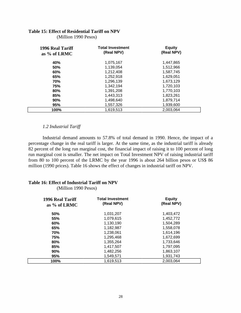
As mentioned above, the lower the ratio of the tariff to the LRMC, the greater the impacton NPV of raising the tariff to the level LRMC. Residential tariffs in 1988 were about 39% ofLRMC. By raising that share to 100% in 1996, one would expect a positive change in NPV.Indeed the results of the sensitivity analysis in Table 15 show a net impact on Total Investmentperspective NPV of about 544 billion pesos or about US$ 177 million when the residential tariffis raised to its LRMC level.
28
Table 15: Effect of Residential Tariff on NPV(Million 1990 Pesos)
1996 Real Tariff as % of LRMC
Total Investment(Real NPV)
Equity(Real NPV)
40% 1,075,167 1,447,86550% 1,139,054 1,512,96660% 1,212,408 1,587,74565% 1,252,918 1,629,05170% 1,296,139 1,673,12975% 1,342,194 1,720,10380% 1,391,208 1,770,10385% 1,443,313 1,823,26190% 1,498,640 1,879,71495% 1,557,326 1,939,600100% 1,619,513 2,003,064
1.2 Industrial Tariff
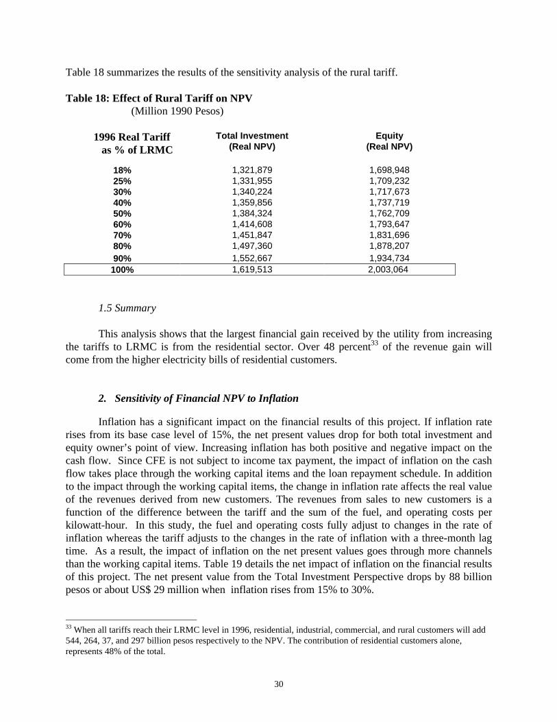
Industrial demand amounts to 57.8% of total demand in 1990. Hence, the impact of apercentage change in the real tariff is larger. At the same time, as the industrial tariff is already82 percent of the long run marginal cost, the financial impact of raising it to 100 percent of longrun marginal cost is smaller. The net impact on Total Investment NPV of raising industrial tarifffrom 80 to 100 percent of the LRMC by the year 1996 is about 264 billion pesos or US$ 86million (1990 prices). Table 16 shows the effect of changes in industrial tariff on NPV.
Table 16: Effect of Industrial Tariff on NPV(Million 1990 Pesos)
1996 Real Tariff as % of LRMC
Total Investment(Real NPV)
Equity(Real NPV)
50% 1,031,207 1,403,47255% 1,079,615 1,452,77260% 1,130,190 1,504,28965% 1,182,987 1,558,07870% 1,238,061 1,614,19675% 1,295,468 1,672,69980% 1,355,264 1,733,64685% 1,417,507 1,797,09590% 1,482,256 1,863,10795% 1,549,571 1,931,743100% 1,619,513 2,003,064

29
1.3 Commercial Tariff
The net impact on Total Investment NPV of raising the commercial tariff from 90 to 100percent of LRMC is about 37 billion pesos or about US$ 12 million. This small amountcompared with the results of the remaining groups of customers is mainly explained by the factthat commercial tariff was very closed to LRMC to start with, and by the fact that demand ofcommercial customers represented only 8.7% of total demand in 1990. The results of thesensitivity analysis of commercial tariff are summarized in Table 17.
Table 17: Effect of Commercial Tariff on NPV(Million 1990 Pesos)
1996 Real Tariff as % of LRMC
Total Investment(Real NPV)
Equity(Real NPV)
50% 1,459,490 1,839,79155% 1,472,892 1,853,46260% 1,486,822 1,867,672
65% 1,501,298 1,882,44170% 1,516,338 1,897,78675% 1,531,962 1,913,72680% 1,548,187 1,930,28185% 1,565,035 1,947,47290% 1,582,524 1,965,31895% 1,600,676 1,983,842100% 1,619,513 2,003,064
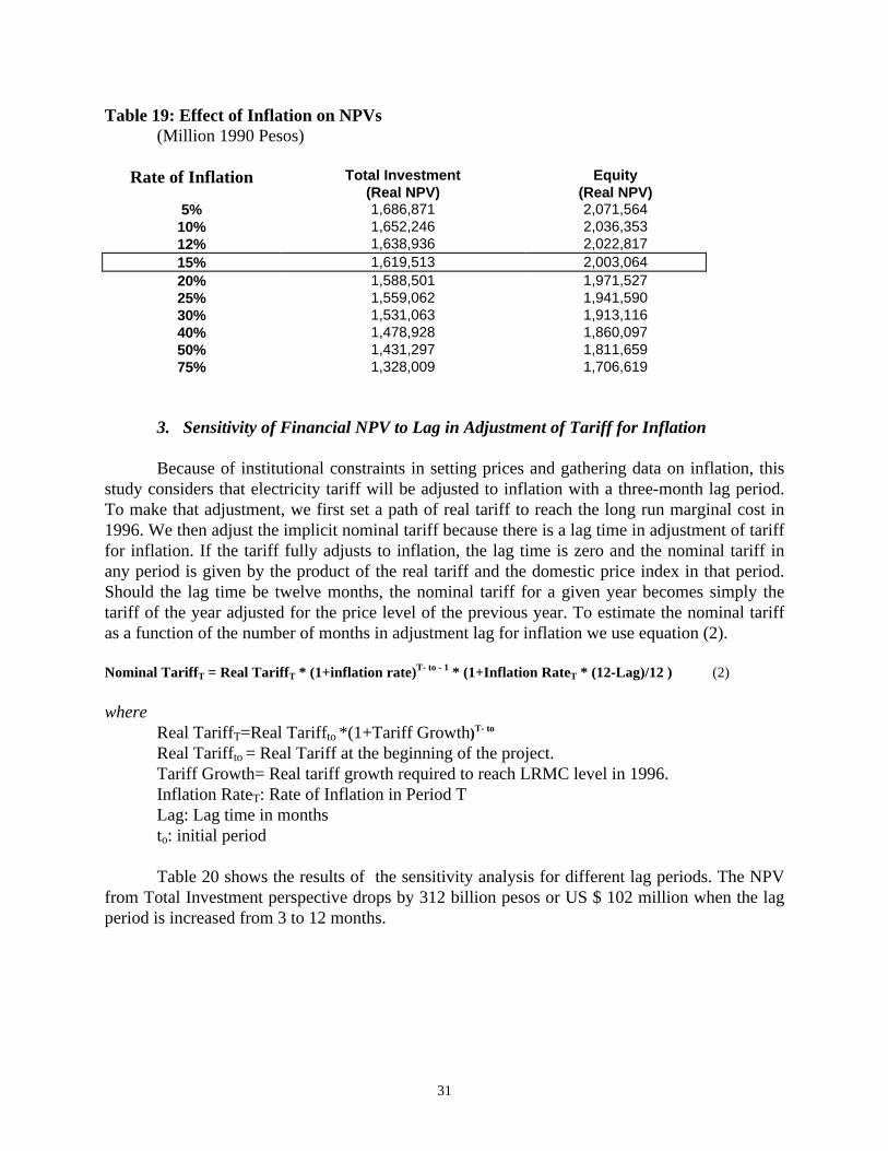
1.4 Rural Tariff
One would expect as in the case of residential customers, a significant impact on the NPVwhen rural tariff increases to their LRMC level because the initial ratio of tariff and LRMC waslow. Although this is the case and the raising of rural tariff to their LRMC level adds about 297billion of pesos or about US$ 97 million to Total Investment NPV, the impact here is lowerbecause rural demand amounts to only 7.9% of total demand in 1990. Consequently, the impacton NPV is smaller even though the initial ratio of tariff and LRMC was 18% for rural customerswhile the same ratio for residential users was 39%.
30
Table 18 summarizes the results of the sensitivity analysis of the rural tariff.
Table 18: Effect of Rural Tariff on NPV(Million 1990 Pesos)
1996 Real Tariff as % of LRMC
Total Investment(Real NPV)
Equity(Real NPV)
18% 1,321,879 1,698,94825% 1,331,955 1,709,23230% 1,340,224 1,717,67340% 1,359,856 1,737,71950% 1,384,324 1,762,70960% 1,414,608 1,793,64770% 1,451,847 1,831,69680% 1,497,360 1,878,20790% 1,552,667 1,934,734100% 1,619,513 2,003,064
1.5 Summary
This analysis shows that the largest financial gain received by the utility from increasingthe tariffs to LRMC is from the residential sector. Over 48 percent33 of the revenue gain willcome from the higher electricity bills of residential customers.
2. Sensitivity of Financial NPV to Inflation
Inflation has a significant impact on the financial results of this project. If inflation raterises from its base case level of 15%, the net present values drop for both total investment andequity owner’s point of view. Increasing inflation has both positive and negative impact on thecash flow. Since CFE is not subject to income tax payment, the impact of inflation on the cashflow takes place through the working capital items and the loan repayment schedule. In additionto the impact through the working capital items, the change in inflation rate affects the real valueof the revenues derived from new customers. The revenues from sales to new customers is afunction of the difference between the tariff and the sum of the fuel, and operating costs perkilowatt-hour. In this study, the fuel and operating costs fully adjust to changes in the rate ofinflation whereas the tariff adjusts to the changes in the rate of inflation with a three-month lagtime. As a result, the impact of inflation on the net present values goes through more channelsthan the working capital items. Table 19 details the net impact of inflation on the financial resultsof this project. The net present value from the Total Investment Perspective drops by 88 billionpesos or about US$ 29 million when inflation rises from 15% to 30%.
33 When all tariffs reach their LRMC level in 1996, residential, industrial, commercial, and rural customers will add544, 264, 37, and 297 billion pesos respectively to the NPV. The contribution of residential customers alone,represents 48% of the total.
31
Table 19: Effect of Inflation on NPVs(Million 1990 Pesos)
Rate of Inflation Total Investment(Real NPV)
Equity(Real NPV)
5% 1,686,871 2,071,56410% 1,652,246 2,036,35312% 1,638,936 2,022,81715% 1,619,513 2,003,06420% 1,588,501 1,971,52725% 1,559,062 1,941,59030% 1,531,063 1,913,11640% 1,478,928 1,860,09750% 1,431,297 1,811,65975% 1,328,009 1,706,619
3. Sensitivity of Financial NPV to Lag in Adjustment of Tariff for Inflation
Because of institutional constraints in setting prices and gathering data on inflation, thisstudy considers that electricity tariff will be adjusted to inflation with a three-month lag period.To make that adjustment, we first set a path of real tariff to reach the long run marginal cost in1996. We then adjust the implicit nominal tariff because there is a lag time in adjustment of tarifffor inflation. If the tariff fully adjusts to inflation, the lag time is zero and the nominal tariff inany period is given by the product of the real tariff and the domestic price index in that period.Should the lag time be twelve months, the nominal tariff for a given year becomes simply thetariff of the year adjusted for the price level of the previous year. To estimate the nominal tariffas a function of the number of months in adjustment lag for inflation we use equation (2).
Nominal TariffT = Real TariffT * (1+inflation rate)T- to - 1 * (1+Inflation RateT * (12-Lag)/12 ) (2)
whereReal TariffT=Real Tariffto *(1+Tariff Growth)T- to Real Tariffto = Real Tariff at the beginning of the project.Tariff Growth= Real tariff growth required to reach LRMC level in 1996.Inflation RateT: Rate of Inflation in Period TLag: Lag time in monthsto: initial period
Table 20 shows the results of the sensitivity analysis for different lag periods. The NPVfrom Total Investment perspective drops by 312 billion pesos or US $ 102 million when the lagperiod is increased from 3 to 12 months.

32
Table 20: Effect of Lag in Adjustment of Tariff for Inflation(Million 1990 Pesos)
Months Total Investment(Real NPV)
Equity(Real NPV)
0 1,730,053 2,115,7711 1,692,843 2,077,8312 1,655,997 2,040,2643 1,619,513 2,003,0646 1,512,195 1,893,6488 1,442,401 1,822,49110 1,373,982 1,752,737
12 1,306,914 1,684,36224 931,647 1,301,819
4. Sensitivity of Financial NPV to Investment Cost Overruns
The investment costs for the base case already includes a contingency cost item. Sincecost overruns is the difference between the investment costs upon realization of the project andthe initial investment cost, the value of cost overruns may be higher or lower than thecontingency cost.
In the base case, the contingency cost represents 11% of total investment. In Table 21below, we vary the percentage of total investment from -10% to 50%. That range includes the11% of the contingency cost. As shown in Table 21, the real cost overrun has a significant impacton the financial result. The financial NPV from Total Investment perspective drops about 182billion pesos or US$ 59 million when costs overruns increase to 20% from the base level of 11%.At the same time this project is quite robust with respect to investment costs. Even if theinvestment cost rise to 50 percent above the original estimates, the financial net present valuefrom the Total Investment perspective would still be positive. The following table shows thesummary of the effect of cost overruns on NPV.
Table 21: Effect of Cost Overrun on NPV(Million 1990 Pesos)
Costs Overruns as% of total investment
Total Investment(Real NPV)
Equity(Real NPV)
-10% 2,044,572 2,429,057-5% 1,943,368 2,327,6300% 1,842,163 2,226,20311% 1,619,513 2,003,06415% 1,538,549 1,921,92320% 1,437,344 1,820,49625% 1,336,139 1,719,07030% 1,234,935 1,617,64340% 1,032,525 1,414,78950% 830,116 1,211,936

33
5. Sensitivity of Financial NPV to Amount of Accounts Receivable
Table 22 indicates that the financial NPV is affected by the size of the accountsreceivable. The Total Investment NPV drops by 200 billion pesos or US$ 65 million when theaccounts receivable are increased from 1.5 months to 3.5 months of annual sales.
Table 22: Effect of Accounts Receivable on NPV (million pesos)
Accounts Receivable (Months) Total Investment Equity1 1,669,541 2,053,740
1.5 1,619,513 2,003,0642.0 1,569,484 1,952,3892.5 1,519,455 1,901,7143 1,469,426 1,851,039
3.5 1,419,397 1,800,3644 1,369,368 1,749,6895 1,269,310 1,648,3386 1,169,253 1,546,988
6. Sensitivity of Financial NPV to Fuel Cost
From 1962 to 1988, the growth in real fuel oil price34 averaged 3.6% with peak rate of40% and 60% respectively in 1974, and 1983. Although there were fuel oil price hikes in someyears, the growth in real fuel oil price tends to be negative in many years. The followingsensitivity analysis considers a range from -5% to 7% change in the level of real fuel oil price forthe life of the project. Changes in the real fuel cost have two effects on the revenues of thisproject. The first effect takes place through the adjustment of long-run marginal costs to changesin real fuel costs. When real fuel cost increases, the long run marginal costs increase and this alsoincreases the savings due to reduction of losses. Moreover, the revenues from the sales to newcustomers and sales due to reduction of outages also increase because the real tariff adjusts tochanges in the long-run marginal cost. The second effect is the impact of the changes in the realfuel cost on the revenues from new customers and from reduction of outages. When real fuel costincreases, the revenues fall because the production cost increases.
In this study, the overall net impact on the NPV of a rise in real fuel cost is positivebecause the first effect dominates the second one. When the real cost of fuel increases by 7%,the NPV from the Total Investment perspective increases by 54 billion pesos or US$ 17.6 millionpesos. Table 23 summarizes the impacts of the level of change in real fuel cost on the net presentvalues in both cases.
34 World Bank, Sectoral Electricity Demand in Mexico, Table A-5, p.38

34
Table 23: Effect Of Fuel Cost On NPV (Million 1990 Pesos)
Change in Level of RealFuel Oil Cost for Entire
Project
Total Investment(Real NPV)
Equity(Real NPV)
-5% 1,580,411 1,962,559-3% 1,596,101 1,978,811-1% 1,611,725 1,994,9970% 1,619,513 2,003,0641% 1,627,284 2,011,1162% 1,635,040 2,019,1513% 1,642,780 2,027,1694% 1,650,504 2,035,1725% 1,658,212 2,043,1586% 1,665,905 2,051,1297% 1,673,583 2,059,083
7. Sensitivity of Financial NPV to Real Exchange Rate
his analysis considers a percentage change in real exchange rate in the year 1990. Afterthis one time change, real exchange rate remains constant throughout the life of the project. Withthat assumption, the burden of the loan repayment in later years is offset by the inflow of the loanin early years so that the resulting impact on the net present value of the project from the equityperspective is reduced.
Long run marginal costs, tariffs, and fuel cost are adjusted to changes in the real exchangerate. Exchange rate is linked to fuel, and marginal costs because of their tradable content. Sincetariffs adjust to marginal cost, changes in real exchange rate also affect the tariff.
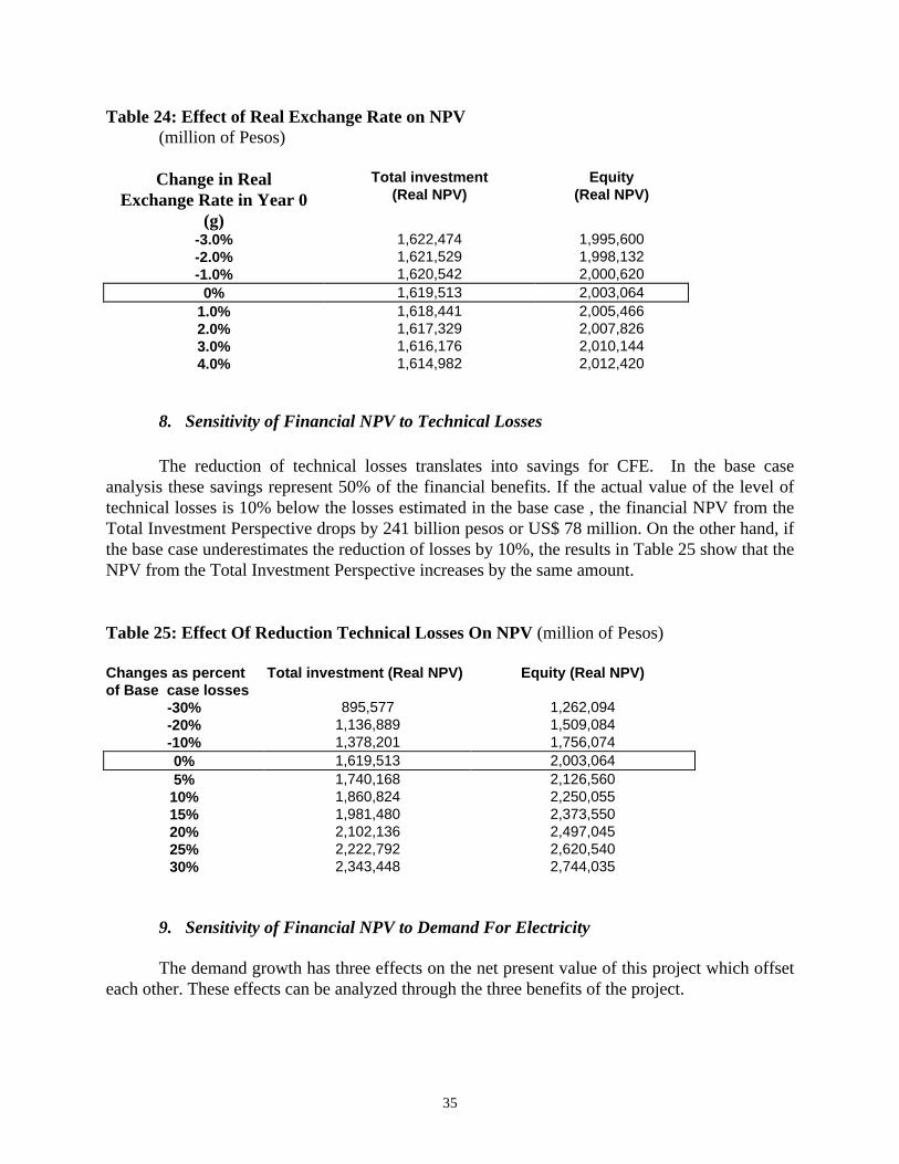
Given the volatile history of real exchange rate and the substantial share of foreign loansin this project, movements in the real exchange rate are expected to have an impact on the projectnet present value. A real devaluation of the domestic currency has two opposing effects on thenet present value. The first effect lowers the net present value because the fuel cost and the debtburden increase. The second effect leads to greater revenues because the level of real tariff, andthe savings resulting from loss reduction increase. In this study, the net impact of a realdevaluation of the domestic currency is a moderate change in net present values. In increasing thereal exchange rate by 3% in 1990, the net present value from the Total Investment perspectivedecreases by 3.4 Billion pesos. Table 24 summarizes the sensitivity analysis of changes in realexchange rate on net present values from both Total Investment and Equity Owner’sperspectives.
35
Table 24: Effect of Real Exchange Rate on NPV(million of Pesos)
Change in RealExchange Rate in Year 0
(g)
Total investment(Real NPV)
Equity(Real NPV)
-3.0% 1,622,474 1,995,600-2.0% 1,621,529 1,998,132-1.0% 1,620,542 2,000,620
0% 1,619,513 2,003,0641.0% 1,618,441 2,005,4662.0% 1,617,329 2,007,8263.0% 1,616,176 2,010,1444.0% 1,614,982 2,012,420
8. Sensitivity of Financial NPV to Technical Losses
The reduction of technical losses translates into savings for CFE. In the base caseanalysis these savings represent 50% of the financial benefits. If the actual value of the level oftechnical losses is 10% below the losses estimated in the base case , the financial NPV from theTotal Investment Perspective drops by 241 billion pesos or US$ 78 million. On the other hand, ifthe base case underestimates the reduction of losses by 10%, the results in Table 25 show that theNPV from the Total Investment Perspective increases by the same amount.
Table 25: Effect Of Reduction Technical Losses On NPV (million of Pesos)
Changes as percentof Base case losses
Total investment (Real NPV) Equity (Real NPV)
-30% 895,577 1,262,094-20% 1,136,889 1,509,084-10% 1,378,201 1,756,0740% 1,619,513 2,003,0645% 1,740,168 2,126,56010% 1,860,824 2,250,05515% 1,981,480 2,373,55020% 2,102,136 2,497,04525% 2,222,792 2,620,54030% 2,343,448 2,744,035
9. Sensitivity of Financial NPV to Demand For Electricity
The demand growth has three effects on the net present value of this project which offseteach other. These effects can be analyzed through the three benefits of the project.

36
First, an increasing demand growth would have no impact on the revenues from newconsumption because the new capacity installed by the project would be utilized completelywhen the project is implemented. When the new capacity due to the project is just enough tosupply the new customers, an increase in the demand for electricity will have no impact on thebenefits from increased consumption by new customers. If however, the project provides capacityin excess of existing demand, an increase in future demand met by the project would generatemore revenues and hence increase the financial benefits. It is assumed in this study that uponcompletion of this project, the new capacity will be completely utilized to reduce part of theexisting shortage and, therefore, any further increase in demand will not be met by the capacityinstalled because of this project.
Second, the effect of demand growth on the revenues from outages reduction is relativelysmall. The revenues from outages reduction are a function of total demand and reduction ofoutages time. We expect that when demand increases the benefits from the reduction of outagesalso increase. To measure the effect of demand growth on the revenues, we need to separate thegrowth of demand in two components. The first component measures the growth due to existingcustomers who are currently affected by outages. The second component measures the growthdue to new customers. Only the first component is used in this study to assess the impact ofdemand on the benefits from the reduction of outages. With the assumption that electricity pricesand income are constant in the “with” and “without” project situations, one can infer that thegrowth in demand due to existing customers is relatively small compared to the growth due tonew customers. Hence, the additional benefits due to demand growth in the case of outagereduction is relatively small.
Third, when the demand increases for a given capacity of transmission network the lossesalso increase. These losses will increase with the demand to a level of reliability admissible bythe utility. Beyond that level of reliability, the utility will not operate its transmission equipment.When demand increases the benefits from reduction of losses will be smaller since an increasingdemand will also increase the losses. Hence, increasing demand has a negative impact on thebenefits derived from reduction of losses. The constraints on the reliability of the transmissionsystem are not incorporated in this study. However, it is assumed that when the project achievesits target level of reliability of the transmission system, the utility will maintain that levelthroughout the life of the project so that any further increase in demand will be met by newequipment. As a consequence, the benefits from the reduction of losses because of this projectwill not be affected by any further growth in demand.
In conclusion, the net of the two opposing effects of the growth in demand on the netpresent value of this project is small.
F. Conclusion of Sensitivity Analysis
As a result of the sensitivity analysis, five variables are identified as risk variablesbecause of their appreciable impact on the financial net present value, while four variables arefound to have moderate impact on the financial results and therefore will not be included in therisk analysis. The risk variables are: rate of inflation, cost overruns, real fuel cost, real exchange
37
rate, and the loss reduction level. The demand for electricity, the size of the accounts receivableare not included in the risk analysis because of their moderate impact on the financial NPV ofthis project. The tariff of electricity, and the lag in adjustment of tariff for inflation are policyvariables and therefore excluded from the risk analysis.
Sensitivity analysis measures only the net impact of changes in one variable at a timewhile others remain constant. Since in reality many variables move together a more complete riskanalysis needs to be undertaken to assess the overall risk associated with the project.
IV. ECONOMIC ANALYSIS35
The appraisal is conducted using the domestic price level of 1990 as the numeraire. Thefirst step in the economic analysis is to determine the economic benefits of additional electricityconsumption of electricity, the economic benefits of loss reduction and outages reduction, andfinally the economic conversion factors for all inputs used in the project.
A. Economic Benefits
1. Economic Benefits from Increased Consumption due to New Customers.
The transmission project will connect new customers to the grid for whom the service ofthe utility would not be available without the project. For these customers, the alternative wouldbe to generate their own electricity by a gasoline or diesel electricity generator. The cost of self-generation with the same quality as the service of the electric utility represents the maximumwillingness to pay for electricity. The benefits of electricity delivered to new customers arevalued at what they would be willing to pay for the incremental energy supplied by this project.
Energy shortage arises because the demand for electricity at the price charged exceeds thesupply of electricity. The current project will increase the capacity to reduce that shortage. Themaximum demand net of losses which will be met by the project in 1993 is 1372 MW.
The economic valuation of electricity, as depicted in figure 2, takes into account theshortage of energy, the rise of electricity prices to their marginal cost level in 1996, and theincrease in capacity due to the project.
The rise in prices does not result from the implementation of this project. The adjustmentof electricity prices to their LRMC level in 1996 is part of the financial rehabilitation agreementsigned between CFE and the government.
The demand for electricity is represented by the curve DD’ in figure 2. If there were anadequate supply of electricity at the price of P0 the quantity of electricity consumed would be Q3.The lack of system capacity to meet total demand forces CFE to ration the supply of electricity. 35 For further discussion of methodology, see Harberger, Arnold and Glenn Jenkins, Manual, “Program onInvestment Appraisal and Management,” Harvard Institute for International Development, 1997.

38
Hence, if we assume that the available supply is rationed over the potential consumers in a wayunrelated to their willingness to pay, the demand curve with rationing becomes DD0. With thegiven supply of electricity and the regulated price of P0, the quantity of electricity consumed isQ0.
Upon completion of the transmission project, the supply of electricity will increase to Q2
and the electricity price will be P1. We calculate the economic value by analyzing first the priceeffect and thereafter the incremental demand effect. When the tariff increases to P1, the quantityof electricity demanded is reduced to Q1 by the present consumers. The quantity of electricityreleased, Q0-Q1, can now be made available to other consumers who are willing to buy electricityat prices from P1 to Pmax. As a result, the effective demand curve rotates to the right and the newdemand curve becomes DD1 while the supply remains at Q0.
If now, additional capacity from the project that is equal to Q2-Q0 is added to the system,the rationing of electricity can be relaxed further. The demand curve with new level of rationingfor the new capacity after the project is implemented is shown as DD2. At a price of P1, theeffective quantity demanded becomes Q2. The economic benefits as a result of additionalcapacity is shown by the area Q0BDCQ2.
Area Q0BDCQ2 = (Pmax + P1)/2 * (Q2-Q0)
The economic benefits per unit of electricity consumed in a situation of shortage, whenrationing is done proportionally, that is now being supplied as a consequence of the project istherefore the average of Pmax and P1 or,
Economic Benefits per kwh = (Pmax + P1)/2 (3)
In this study, we assumed a linear demand curve with a constant price intercept, which isthe maximum willingness to pay (Pmax). With that assumption, the economic benefits perkilowatt-hour may change only with the real tariff. If however, we allow a change in the priceintercept, the economic value would also change with the maximum willingness to pay. The firstapproach, a linear demand curve with constant price intercept or a semi-log curve yields lowerestimates of the benefits. The second approach, a linear demand curve with a price intercept thatincreases overtime or a constant elasticity curve will give higher estimates of the benefits. Sincewe choose in this study a linear demand curve with a constant price intercept, the economic valueper unit of energy shortage calculated may be lower than the actual economic benefit. It isassumed in this study that the price of electricity will gradually increase in real terms to reach thelong run marginal cost level in 1996. Because of that change in prices, the economic value perunit of electricity consumed in a situation of shortage will also increase.

39
Figure 2: Economic Value Of Electricity due to increased consumption by new customers.
The maximum willingness to pay for electricity (Pmax) with the same quality of power asprovided by a power company with adequate reserves can be measured by the cost of own-generation plus backup generation. To calculate the cost of self-generation, which is about 903.5pesos or US$ 0.294 per Kwh, the following procedure has been used.
The capital cost of a 10HP gasoline power generator in Mexico in 1996 was US$19,174or US$ 15,598 when expressed in 1990 prices. The capacity cost per Kilowatt36, $2,091.7 perKilowatt, is determined as the ratio of the cost and the capacity of the generator. The annualizedcapital cost37, $370.2, is calculated with an economic life of 12 years, and a discount rate of 12%.The capital cost per Kilowatt-hour38 is found to be US$0.0845.The backup factor, the ratio of thecapital cost and total generation cost, is US$ 0.403. The generator consumes 1.17 gallon perhour39. At a price of 80 cents per gallon, it costs $0.12540 to produce one Kilowatt-hour. The totalown-generation cost, $0.210/kwh, is the sum of the fuel and capacity cost per Kilowatt-hour. 36 Capacity cost per Kw = cost of generator/capacity of generator = 15,598/(10*0.7457) =$2091.7/Kw. 1HP=0.7457Kw.37 Annualized cost = PMT(12%,10,-2091.7). PMT is an Excel function for calculating the payment of a loan basedon constant payments and a constant interest rate.38 Capital cost per Kwh = Annualized capital cost/(8760*Load Factor). The load factor is taken as 50%.39 Fuel consumption of the generator is 7 gallon for 6 hours.40 Fuel cost per Kwh= Fuel cost/Gallon* Fuel consumption/capacity of generator =0.8*1.1667/(10*0.7457)
Q 2
P 1
O
Economic Value Of
C
Q 1
B
D
D 2D 1D0
A
Q 3
S
D’
Quantity of Electricity
Q0
Pmax
P0
Electricity

40
The maximum willingness to pay41 is $0.294 per Kilowatt-hour. Table 26 summarizes the resultsof total own-generation and the maximum willingness to pay.
Table 26: Own-Generations: Average tariff and Willingness To Pay in Mexico(1990 Prices)42
Capital cost of a 10 HP gasoline power generator in Mexico in 1990 (US$)* 15,598Generating Capacity (kW) 7.5Capacity Cost ($/kW) 2091.7Annualized Capacity Cost ($/kW, 10 years life, 12%) 370.2Load Factor 50%Capital Cost per kWh 0.0845Fuel Consumption (gallon per hour, note: 7 gallon per 6 hours) 1.1667Fuel Cost ($/gallon) 0.8Fuel Cost ($/kWh) 0.125Total Own-generation Cost ($/kWh) 0.210Maximum Willingness To Pay (1990 $/kWh) 0.294Maximum WTP (1990, m. Ps/MWH) 0.9035Based on 1997 cost in Mexico.
The economic benefits to new customers are calculated as the product of newconsumption and the benefit per unit of shortage as defined in equation (3). The economic costsof providing the incremental demand to new customers, include fuel and operating costs. Thedifference between the benefits and costs is multiplied by the share, 28.77%, of the capital cost oftransmission to the total capital cost of the electricity system to estimate the final benefits thataccrue due to the transmission project.
Calculation of the economic value of electricity from increased consumption due to newcustomers43 from 1990 to 1993 is shown in Table 27.
41 Maximum willingness to pay = (1+backup power factor)*Total generation cost=(1+0.403)*0.210=0.29442 See Annex 17.43 For the entire life of the project, refer to Annex 16B.

41
Table 27: Economic Value of Electricity from Increased Consumption due to NewCustomers. (million of 1990 Pesos per Mwh)
1990 1991 1992 1993
Maximum willingness to pay (Pmax) 0.903 0.903 0.903 0.903
Average electric tariff P1 0.114 0.133 0.155 0.182
Economic value per unit of shortage44 (a) 0.509 0.518 0.529 0.543
Economic value of fuel per Mwh45 (b) 0.151 0.151 0.151 0.151
Economic Value of operating cost perMwh46 (c)
0.0017 0.0017 0.0017 0.0017
Share of transmission to overall value of economicbenefits 47 (d)
0.287 0.287 0.287 0.287
Economic value of electricity due totransmission project (million Pesos)48
133,730 256,786 348,169 619,765
Economic value of electricity due totransmission project49 (US$ million)
43.55 83.6 113.37 201.8
The present value of economic benefits from increased consumption due to new customers is4,497 billion pesos or US$ 1,464 million.
2. Economic Benefits due to Reduction of Losses
In addition to the benefits from increased consumption, the Mexican economy also gainsfrom the resources saved because the project lowers the technical losses. The resources savedinclude fuel, operating and generation capacity costs. The conversion factors for these items are1.253, 0.809, 0.999 respectively.
44 Economic Value per unit of shortage = (Pmax+P1)/2 or the average of the maximum willingness to pay and theelectric tariff.45 Economic value of fuel per Mwh= Financial value per Mwh * Conversion factor for fuel.The financial value of fuel per Mwh estimated by CFE equals 86.6 pesos per kwh. The conversion factor for fuelcalculated in Annex 15D of this study is 1.253.46 Economic value for operating costs per Mwh= Financial value per Mwh* Conversion factor for operating items.This conversion factor 0.809, is calculated in Annex 16A.47 This share is calculated using equation 4.48 Economic value from consumption by new customers = [a-(b+c)/(1-losses)]* d *energy sold to new customers.Losses equal 15% of total generation.49 The benefits expressed in pesos are converted in dollars using the real exchange 3,071 pesos/ 1US$ in 1990.

42
The present value of the economic benefits from loss reduction is estimated to be 1,558billion pesos or US$ 507 million. Most of these benefits come from the savings in fuelconsumption. The fuel saved from the reduction of losses is now available for export and theeconomy gains the foreign exchange and the foreign exchange premium for exporting thatamount of fuel.
3. Economic Benefits From Reduction of Outages.
The economic benefits from reduction of outages are estimated by multiplying thedifference in energy provided in the “without” and “with” project by the cost of power outages.The opportunity cost of power outages is estimated from data given in Table 28. The cost perkwh remains constant throughout the life of this project.
Table 28: Outage Costs by User50 Categories.
Users US$/Kwh
Residential 0.70Industrial 1.20Commercial 0.75Rural 0.75Other 0.50
Weighted Total 1.00
CFE has estimated, based on computer models, a total annual reduction of 102 minutes induration of outages as a result of the implementation of the transmission project by the year1993. From 1990 to 1992, outage time reduction is estimated prorata of the total demand in eachyear since the losses are a function of the total demand of the system. From 1993 to the end ofthe project, it is assumed that the project will result in a reduction in outage time of 102 minutes.The present value of the benefits from reduction of outage time is 267 billion pesos or US$ 87millions.
4. Summary of Present Values of Gross Financial and Economic Benefits
As shown in Table 29, the economic benefits from increased consumption due to newcustomers are 4,497 billion while the financial benefits are 2,230 billions pesos. The economicbenefits due to loss reductions amount to 1,558 billion pesos while the financial benefits amountto 2,413 billion pesos. The economic benefits from outage reduction amount to 314 billion whilethe financial benefits are only 216 billion pesos.
50 Luis Gutierrez, Economic Analysis of a Power Investment Program, p8.

43
Table 29: Present Values of Gross Financial and Economic Benefits (billion of Pesos)
Financial Benefits Economic Benefits
Benefits from IncreasedConsumption due to newcustomers
2,230 4,497
Benefits from Reduction ofTechnical losses
2,413 1,558
Benefits from reduction ofoutages
216 314
The economic benefits from reduction of technical losses are lower than the financialbenefits because the impact of a higher economic discount rate outweighs the gains from foreignexchange premium and the gains from the reduction of fuel subsidies for electricity generation. Alow financial discount rate accounts for about 1,100 billion51 pesos that contributes to a greaterfinancial net present value. Therefore, at the same economic discount rate, the economic netpresent value would be higher by 245 billion Pesos52. The amount of 245 billion pesos comesmainly from the net gain from foreign exchange premium and from the reduction in fuelsubsidies.
51 The present value of the financial benefits due to reduction of losses using the economic discount rate is 1313billion. The present value of the financial benefits due to reduction of losses using the financial discount rate is 2413billion The difference of the present values at the financial and at the economic discount rate is 1100 billion pesos.52 The present value of the economic benefits due to loss reduction using the economic discount rate is 1558 billion.At the same economic discount rate, the present value of the economic benefits due to loss reduction would begreater than the present value at financial discount rate by 245 billion, which equals 1558-1313 billion pesos.
44
B. Economic Costs of Foreign Exchange and Capital
1. Economic Cost of Foreign Exchange
The economic cost of foreign exchange is calculated in Annex 15B. The economic cost offoreign exchange is found to be 10.6% higher than the official exchange rate. This premium isdue partly to the impact of net import tariffs and indirect taxes (VAT and excises).
2. Economic Cost of Capital
The economic cost of capital for Mexico is estimated to be 12.4%. This cost isdetermined as a weighted average of the different domestic net-of-tax saving rates, the gross-of-tax returns on investment for the different sectors, and the marginal costs of foreign borrowing.Annex 15C gives the assumptions and the computation of the economic cost of capital.
C. Estimates of Economic Costs of Inputs
1. Basic Conversion Factors
The investment and operating costs of the project consist of the costs of individual itemssuch as freight, insurance, non- tradable and tradable materials and equipment, and tradable fuel.Before calculating the conversion factors for the investment and operating items, we determinethe basic conversion factors for the above individual items.
The following assumptions were made for labor, import tariff, local freight and insurance,and non-tradable materials.
Economic Cost of Labor
From a previous study53 done by the World Bank we derived the composition of skilledand unskilled labor involved in the transmission project. Skilled labor represents about 58% ofthe total labor. No further information regarding the prevailing market wage, the existence of aprotected labor market, the distortions in the labor market or the chance that skilled labormigrated to the project area, was readily available. As an alternative, we used the conversionfactors obtained from a study54 done by the Inter-American Development Bank in 1988. Theconversion factors for skilled and unskilled labor were respectively 0.734 and 0.482.
53 Luis Gutierrez ,Economic Analysis of a Power Investment Program, January 1991.54 National Finananciera, Los precios de cuenta en Mexico 1988, 2nd ed., p77.

45
Import Tariff
The actual import tariff for different categories of the tradable components were notavailable. The average import tariff calculated in Annex 15B for 1990 is 10%. This rate isappropriate given the prevailing rates applicable after the March 1989 Trade Tariff Regime55.
Local Freight and Insurance
The local freight and insurance costs were also estimated to be 10% of the CIF value.The supply and demand weights for freight and insurance were assumed to be 80% and 20%respectively. We also considered that freight and insurance were made of 50% tradablecomponents. The weights are the proportions of the quantity of the local freight and insurancepurchased by the project that are accommodated by increased supply and decreased demandrespectively.
Non-tradable materials
We used equal weights of 50% each for the supply and demand, and 20% as theproportion of tradable components used in the supply of these items. The weights are theproportions of the quantity of non-tradable purchased by the project that are accommodated byincreased supply and decreased demand respectively.
The low weight for demand in local freight is attributable to the weak response ofdemanders of these items. In other words, most of the freight, insurance and non-tradabledemanded by the project is accommodated by an increase in the supply of local freight bysuppliers.
With the above assumptions, we calculated the basic conversion factors, makingappropriate adjustments for the foreign exchange premium, freight and insurance, tradablematerials and equipment, non-tradable materials, and tradable fuel. The calculations and resultsof the basic conversion factors are summarized in Annex 15D.
The next step is to calculate the conversion factors for investment and operating items.
2. Conversion Factors for Investment Cost Items
Investment costs comprise transformers, breakers, transmission lines, and high voltagefeeders. Each investment item is made of a share of tradable and non-tradable materials, and ashare of skilled and non-skilled labor. Given the shares and the basic conversion factors, weestimated the conversion factor for each investment line as the weighted average of theconversion factors of its components.
55 World Bank, Mexico Tax Reform for Efficient Growth, Report No 8097-ME, p.78.

46
3. Conversion Factors for Operating Cost Items
Operating Expenses
The conversion factor for operating and maintenance is the weighted average of theconversion factors for labor, tradable and non tradable materials.
Fuel Costs
Fuel is an input in this project that is currently being heavily subsidized when used inelectricity generation. Fuel used in the project reduces the quantity available for export and,hence, results in a loss of foreign exchange. Therefore, the economic cost of fuel is measured asthe foregone benefits due to the reduction of fuel exports. The conversion factor for fuel,calculated in Annex 15 D, is 1.253.
4. Conversion Factors for Working Capital Items
Accounts Payable
As this item constitutes a percentage of operating expenses, the conversion factor is thesame as that for the operating expenses.
Accounts Receivable and Cash Balances
Accounts receivable result from the sales to new customers and the sales due to outagesreduction. Therefore, the economic value of per unit of receivable is the weighted average of theeconomic benefits per unit of increased sales to new customers and per unit of sales induced byoutages reduction.
The conversion factor for changes in cash balances is taken simply as 1.0.
D. Environmental Impact of the Project
The potential environmental impacts for a transmission project include electromagneticradiation, noise, erosion and land use56. While a few studies have attempted to relateelectromagnetic radiation from transmission lines to cancer in humans, there is no reliableevidence to substantiate this conclusion. The erosion from temporary or permanent earthworksreduce soil levels and affect agriculture and terrestrial ecosystems. The right-of-way land for thetransmission line could displace households or limit land use for agriculture and other productiveuses. Although these environmental stressors affect the results of the project, no attempt wasmade in this appraisal to account for these stressors because of the lack of quantitative data ofthese stressors and because of their small effect on environment. However, we provide in AnnexA the taxonomy for evaluating potential impacts of the environmental stressors in a transmissionproject. 56 Economic Evaluation of Environmental Impacts, Asian Development Bank, p.62

47
E. Results of Economic Analysis
The economic value per unit of shortage, adjusted for fuel cost and the marginal capitalcost of the transmission, is used to calculate the economic benefits due to additionalconsumption. The economic benefits from outages reduction are valued at the cost of outages.For other items, the conversion factors are applied to the real cash flow from the total investmentpoint of view to obtain the economic cash flow statement presented in Table 30. The economicnet present value of the transmission project is 3,894 billions of pesos or US$ 1,268 million,indicating that the project adds substantial net wealth to the Mexican economy.

48
TABLE 30: STATEMENT OF ECONOMIC BENEFITS AND COSTS (1990 prices)(Million of Pesos)
1990 1991 1992 1993 1994 1995 1996 1997 1998 2024 2025RECEIPTSREVENUESales to new customers 133730 256786 348169 619765 625028 637306 657868 651318 644180 499505Lines and Transformers Losses reductions 98464 105375 127370 151812 152153 153190 154818 160835 167895 545968Change in accounts receivable -7662 -6661 -4505 -13520 1148 984 822 255 276 1377 24493Sales due to Reduction of Outages 5613 11477 16460 31157 32004 32927 33899 35440 37252 140919 0
Total Benefits 230144 366978 487495 789213 810332 824408 847408 847848 849603 1187768 24493EXPENDITURESInvestment CostsEquipment and MaterialsTransformers 0.997 27205 135756 67878 41750Breakers 0.933 20426 102132 51192 30766Transmission lines 0.991 103125 506252 254733 166340High Voltage Feeders 0.991 43125 215894 108483 63482Labor Costs Skilled 0.734 11486 56879 28574 17908Unskilled 0.482 5388 26683 13404 8401Sub-Total 210757 1043597 524264 328647Contingency as costs overruns 0.943 23180 114786 57663 36139 Total Subprogram Investment 233937 1158383 581928 364787Operating costsMaintenance Expenses due to sales from outage reduction0.809 14 28 40 76 78 81 83 87 91 346Fuel costs due to outages reduction 1.253 1217 2488 3568 6753 6937 7137 7348 7682 8075 30546 0Total System Costs 1230 2516 3608 6830 7016 7218 7431 7769 8166 30891 0Bad Debt 0 0 0 0 0 0 0 0 0 0 0 0Working capitalChange in accounts payable 0.809 -15304 -15299 -12728 -31908 -6134 -6162 -6229 -7148 -7040 -3990 42538Change in cash balance 1.000 -18907 -18900 -15725 -39419 -7578 -7613 -7696 -8831 -8698 -4929 52552Total change in working capital 3603 3602 2996 7512 1444 1451 1466 1683 1657 939 -10014VATIncome TaxesEnvironmental impact of Land Use 42537 42537 42537 42537 42537 42537 42537 42537 42537 42537 42537Total Costs 281307 1207037 631070 421665 50997 51206 51435 51989 52361 74367 32523NET ECONOMIC BENEFITS -51163 -840059 -143575 367548 759336 773202 795973 795859 797242 1113401 -8030NPV (in Million Pesos) 12% 3,893,828NPV (in Billion Pesos) 3,894NPV (in US$ Million) 1,268
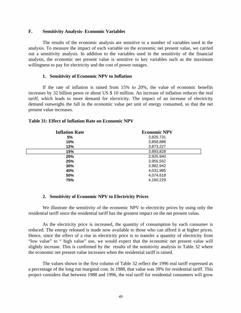
49
F. Sensitivity Analysis- Economic Variables
The results of the economic analysis are sensitive to a number of variables used in theanalysis. To measure the impact of each variable on the economic net present value, we carriedout a sensitivity analysis. In addition to the variables used in the sensitivity of the financialanalysis, the economic net present value is sensitive to key variables such as the maximumwillingness to pay for electricity and the cost of power outages.
1. Sensitivity of Economic NPV to Inflation
If the rate of inflation is raised from 15% to 20%, the value of economic benefitsincreases by 32 billion pesos or about US $ 10 million. An increase of inflation reduces the realtariff, which leads to more demand for electricity. The impact of an increase of electricitydemand outweighs the fall in the economic value per unit of energy consumed, so that the netpresent value increases.
Table 31: Effect of Inflation Rate on Economic NPV
Inflation Rate Economic NPV5% 3,820,73110% 3,858,88812% 3,873,22715% 3,893,82820% 3,925,94025% 3,955,55230% 3,982,94240% 4,031,98550% 4,074,61875% 4,160,229
2. Sensitivity of Economic NPV to Electricity Prices
We illustrate the sensitivity of the economic NPV to electricity prices by using only theresidential tariff since the residential tariff has the greatest impact on the net present value.
As the electricity price is increased, the quantity of consumption by each consumer isreduced. The energy released is made now available to those who can afford it at higher prices.Hence, since the effect of a rise in electricity price is to transfer a quantity of electricity from“low value” to “ high value” use, we would expect that the economic net present value willslightly increase. This is confirmed by the results of the sensitivity analysis in Table 32 wherethe economic net present value increases when the residential tariff is raised.
The values shown in the first column of Table 32 reflect the 1996 real tariff expressed asa percentage of the long run marginal cost. In 1988, that value was 39% for residential tariff. Thisproject considers that between 1988 and 1996, the real tariff for residential consumers will grow
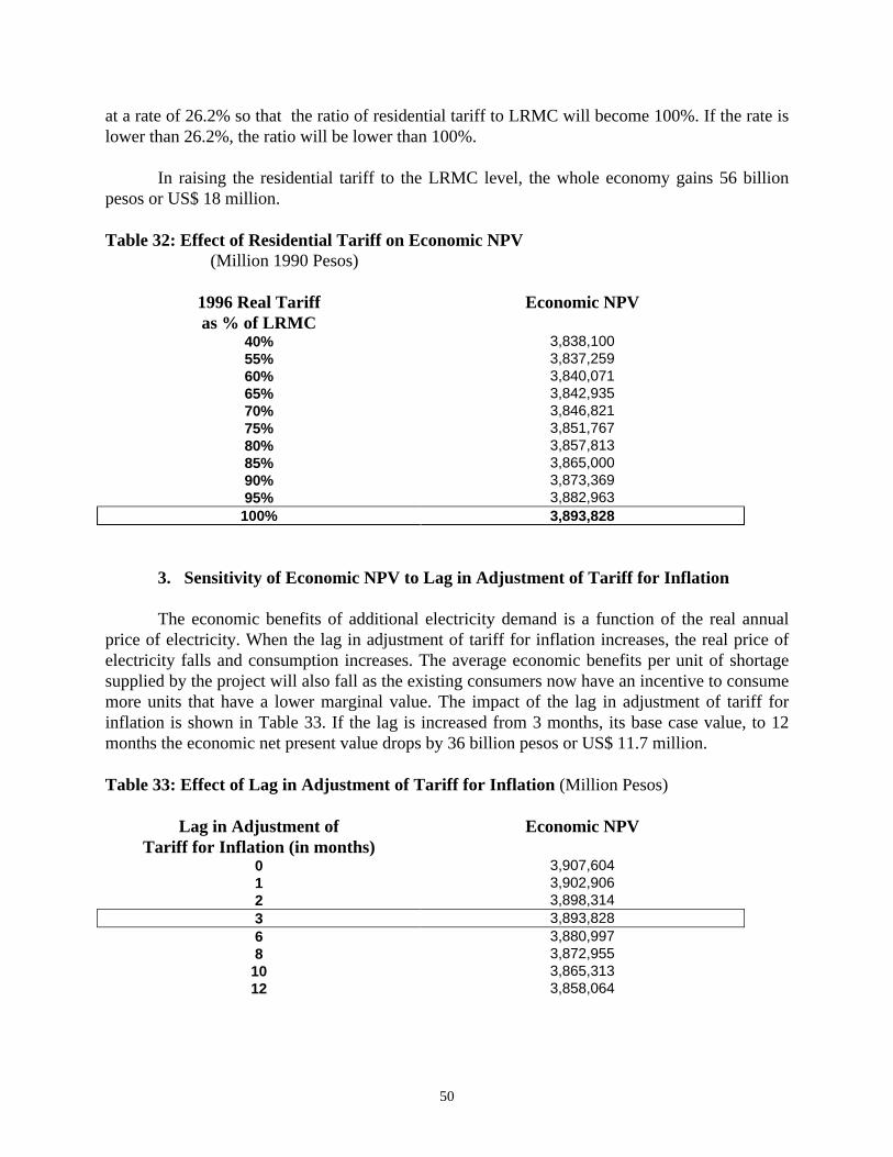
50
at a rate of 26.2% so that the ratio of residential tariff to LRMC will become 100%. If the rate islower than 26.2%, the ratio will be lower than 100%.
In raising the residential tariff to the LRMC level, the whole economy gains 56 billionpesos or US$ 18 million.
Table 32: Effect of Residential Tariff on Economic NPV(Million 1990 Pesos)
1996 Real Tariffas % of LRMC
Economic NPV
40% 3,838,10055% 3,837,25960% 3,840,07165% 3,842,93570% 3,846,82175% 3,851,76780% 3,857,81385% 3,865,00090% 3,873,36995% 3,882,963100% 3,893,828
3. Sensitivity of Economic NPV to Lag in Adjustment of Tariff for Inflation
The economic benefits of additional electricity demand is a function of the real annualprice of electricity. When the lag in adjustment of tariff for inflation increases, the real price ofelectricity falls and consumption increases. The average economic benefits per unit of shortagesupplied by the project will also fall as the existing consumers now have an incentive to consumemore units that have a lower marginal value. The impact of the lag in adjustment of tariff forinflation is shown in Table 33. If the lag is increased from 3 months, its base case value, to 12months the economic net present value drops by 36 billion pesos or US$ 11.7 million.
Table 33: Effect of Lag in Adjustment of Tariff for Inflation (Million Pesos)
Lag in Adjustment ofTariff for Inflation (in months)
Economic NPV
0 3,907,6041 3,902,9062 3,898,3143 3,893,8286 3,880,9978 3,872,95510 3,865,31312 3,858,064

51
4. Sensitivity of Economic NPV to Investment Cost Overruns
The economic net present value drops by 250 million pesos or US$ 81.4 million wheninvestment cost overruns increase from 11% to 25% of total investment. The economic netpresent value, however, remains still highly positive even if investment cost overrun is as high as50% of total investment. Table 34 summarizes the impact of cost overruns on economic netpresent value.
Table 34: Effect of Cost Overrun on Economic NPV(Million Pesos)
Investment Cost Overrunas % Total Investment
Economic NPV
-10% 4,268,545-5% 4,179,3270% 4,090,109
11% 3,893,82815% 3,822,45420% 3,733,23525% 3,644,01730% 3,554,79940% 3,376,36250% 3,197,925
5. Sensitivity of Economic NPV to Fuel Cost
The change in real fuel cost has three impacts on the economic net present value. First, anincrease in fuel price has a positive impact on the value of savings due to loss reduction. With thereduction of technical losses, the amount of fuel used to generate the same quantity of electricitydelivered to customers drops. When the world price of fuel oil increases, the quantity of fuelsaved because of the reduction of losses can be now exported and the economy gains the foreignexchange savings from the export of the fuel. Second, an increase in fuel price reduces the neteconomic benefits derived from new customers as the cost of generation increases. Third, anincrease in fuel price also raises the long run marginal costs and because of that the tariff alsoincrease because the tariff adjusts to the long run marginal costs. This third impact has a positiveeffect on the net present value because the revenues from new consumers increase. The net effectof the changes in the real fuel price is uncertain. In this study, the net effect is negative as shownin Table 35. The economic net present value decreases when the level of real fuel cost increases.The net present value decreases by 18 billion pesos when the level of fuel cost rises to 3%. Table35 summarizes the effect of fuel oil prices on the economic net present value.

52
Table 35: Effect of Fuel Cost on Economic NPV(Million Pesos)
Change In Average Real Fuel Oil Costas percent of Base Case Fuel Cost
Economic NPV
-5% 3,924,400-3% 3,912,136-1% 3,899,9200% 3,893,8281% 3,887,7482% 3,881,6793% 3,875,6224% 3,869,5755% 3,863,5396% 3,857,5137% 3,851,498
6. Sensitivity of Economic NPV to Real Exchange Rate
An increase in the real exchange rate has three effects on the net present value of theproject. The first effect is to increase the net present value because the savings due to lossreduction are higher. These savings comprise the fuel, the operating, and the capacity costs ofgeneration. The second effect on the net present value is also positive. Long run marginal costsadjust upward with an increase of the real exchange rate. Real tariff also go up with an increaseof long run marginal costs. A rise of 1% of the real exchange rate leads to an increase of 0.7%57
of the real tariff. High real tariff translates into high economic value per unit of electricityconsumed by new customers because the average willingness to pay is a function of the realprice. The third effect of an increase of the real exchange rate on the net present value isnegative. When the real exchange rate rises, the cost of the fuel expressed in domestic currencyincreases. Such an increase of the cost of fuel leads to an increase of the generation cost andreduces the net present value.
In this study, a real devaluation has a moderate negative impact on the economic NPV.As illustrated in Table 36, the economic net present value decreases when the real exchange ratesrise. When the real exchange rate rises by 1% a year, the economic net present value decreasesby 20 billion pesos or US$ 6.5 million.
57 It is assumed in this study that 70% of the investments items of this project are tradable, and hence only thatportion is affected by changes in real exchange rate.

53
Table 36: Effect of Annual Changes in the Real Exchange Rate on Economic NPV (Million Pesos)
Annual Changes inReal Exchange Rate (#Ps/$)
Economic NPV
-3.0% 3,954,828-2.0% 3,934,482-1.0% 3,914,149
0% 3,893,8281.0% 3,873,5192.0% 3,853,2233.0% 3,832,9374.0% 3,812,663
7. Sensitivity of Economic NPV to Technical Losses
As shown in Table 37, the economic net present value increases with the reduction oflosses. If the reduction of technical losses is 5% higher than the losses in the base case, theeconomic net present value increases by 77 billion pesos or US$ 25 million. Again these benefitscome mainly from the foreign exchange savings and foreign exchange premium because the fueloil saved can be exported.
Table 37: Effect of Technical Losses Reduction on Economic NPV(Million Pesos)
Changes as percentof Base case losses
Economic NPV
-30% 3,426,457-20% 3,582,247-10% 3,738,0380% 3,893,8285% 3,971,72410% 4,049,61915% 4,127,51420% 4,205,40925% 4,283,30530% 4,361,20035% 4,439,095
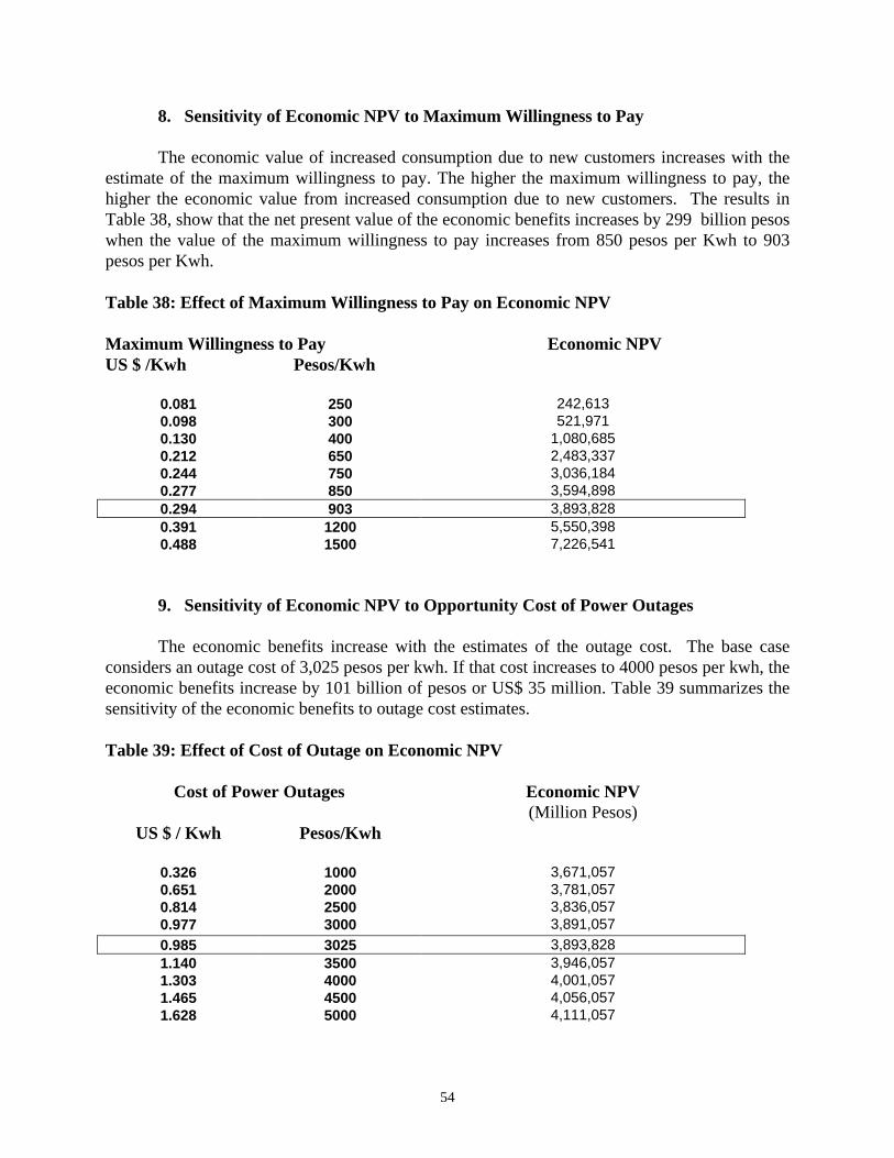
54
8. Sensitivity of Economic NPV to Maximum Willingness to Pay
The economic value of increased consumption due to new customers increases with theestimate of the maximum willingness to pay. The higher the maximum willingness to pay, thehigher the economic value from increased consumption due to new customers. The results inTable 38, show that the net present value of the economic benefits increases by 299 billion pesoswhen the value of the maximum willingness to pay increases from 850 pesos per Kwh to 903pesos per Kwh.
Table 38: Effect of Maximum Willingness to Pay on Economic NPV
Maximum Willingness to Pay Economic NPVUS $ /Kwh Pesos/Kwh
0.081 250 242,6130.098 300 521,9710.130 400 1,080,6850.212 650 2,483,3370.244 750 3,036,1840.277 850 3,594,8980.294 903 3,893,8280.391 1200 5,550,3980.488 1500 7,226,541
9. Sensitivity of Economic NPV to Opportunity Cost of Power Outages
The economic benefits increase with the estimates of the outage cost. The base caseconsiders an outage cost of 3,025 pesos per kwh. If that cost increases to 4000 pesos per kwh, theeconomic benefits increase by 101 billion of pesos or US$ 35 million. Table 39 summarizes thesensitivity of the economic benefits to outage cost estimates.
Table 39: Effect of Cost of Outage on Economic NPV
Cost of Power Outages Economic NPV(Million Pesos)
US $ / Kwh Pesos/Kwh
0.326 1000 3,671,0570.651 2000 3,781,0570.814 2500 3,836,0570.977 3000 3,891,057
0.985 3025 3,893,8281.140 3500 3,946,0571.303 4000 4,001,0571.465 4500 4,056,0571.628 5000 4,111,057

55
G. Conclusion from Economic Analysis
The main conclusion from the economic analysis and the sensitivity tests done on it isthat this project is highly attractive. Although each of the key input variables have been changedacross a wide range of values, the economic net present value never becomes negative. It is clearthat certain variables are more important in determining the final outcome than others. Theability of this project to actually cut technical losses, the willingness to pay for electricity, thecost of power outages, the cost overruns, the real exchange rate, and the rate of inflation inMexico all cause large changes in the economic net present value of the project. The impact ofthe other variables is less significant.
V. DISTRIBUTIVE ANALYSIS
A distributive analysis was conducted to determine the externalities generated by theproject and to identify who benefits and who loses from these externalities. The statement ofexternalities results from the difference between the economic and financial cash flowstatements.
The NPV of externalities is calculated as follows.NPV of externalities = NPV of economic cash flows - NPV of financial cash flows;
all NPVs estimated at the same discount rate, that is, the economic or social cost of capital..
Applying the above formula, we have
NPV of externalities = 3,893,828- 910 = 3,892,918 (million 1990 pesos).
The total benefits of the project are equal to the financial NPV of the project plus theexternalities. Table 40 summarizes the allocation of these externalities to the government, theconsumers, and the labor.
A. Distribution of Project Net Benefits
Column 1 of Table 40 shows that the net benefits to the government is positive . The netgains accruing to the government are of the order of 652 billion pesos or US$ 212 million. Thebenefits to the government come from 523 billion pesos from taxes and additional value addedtaxes on increased consumption of electricity, and 245 billion pesos from the foreign exchangesavings and foreign exchange premium made available because the fuel saved by the reduction oflosses can now be exported. The loss to the government includes 80 billion of grants, 13 billionof forgone foreign exchange premium because of the incremental consumption of fuel due toreduction of outages, and 23 billion in change in account payable.

56
Table 40: Distribution of Project Net Benefits (Million of 1990 pesos)
Government (1) Consumers (2) Labor (3) Total (4)
Benefits Sales to New Customers 3,271,414 3,271,414 Losses reduction 245,065 245,065Sales due to Reduction ofoutages
209,451 209,451
Accounts receivable 82,184 82,184Government Grants -79,696 -79,696Consumers contributions -60,162 -60,162
CostsTransformers 764 764Breakers 12,424 12,424Transmission lines 7,777 7,777High voltage feeders 3,261 3,261Skilled labor 35,248 35,248Unskilled Labor 49,035 49,035Contingency as overruns 10,526 1,435 11961Maintenance cost due tooutages reduction
181 181
Fuel cost due to reductionof outages
-13,768 -13,768
Bad debt 31,192 31,192Change in accounts payable -22,994 -22,994VAT 488,222 488,222Environment cost -378,638 -378,638Net Benefits 651,762 3,155,441 85,718 3,892,921
Reconciliation of Economic, Financial and Distributive Analysis.
The economic net present value equals the financial net present value determined at theeconomic discount rate plus the sum of the distribution impacts induced by the project.
Economic NPV = Financial NPV + PV Externalitiesat economic discount rate at economic discount rate at economic discount rate
3,893,828 = 910 3,892,929
B. Conclusion of Distributive Analysis
Consumers gain most from this project, approximately 3,155 billion pesos or US$ 1,027million, mainly due to the electricity consumption of the newly connected consumers and theavoidance of outages. New consumers get a large amount of the economic benefits because the

57
average willingness to pay for electricity is high. In addition to these benefits, all consumers gainfrom the reduction of the frequency and duration of outages.
The government gains about 652 billion pesos or US$ 212 million which come primarilyfrom foreign exchange savings, foreign exchange premium, and taxes.
The labor, especially the workers at CFE, gains 86 billion Pesos or US$ 28 million.
The present value of the net benefits to consumers is very substantial at 3,155,441 millionpesos (US$ 1,027 million). In principle it would be a reasonably easy task to allocate thesebenefits amongst the various income groups. Unfortunately, the requisite information is presentlynot available for this project.
VI. RISK ANALYSIS OF FINANCIAL AND ECONOMIC RETURNS
The base case gives a single value for the forecast of either the financial or economicNPV. Sensitivity analysis helps to identify variables that may have a major impact on thefinancial and economic results. Although a sensitivity analysis provides useful insights about thefinancial and economic returns of a project, a risk analysis will allow us to evaluate the spread ofthe returns when the effect of the individual variables are combined. To do so, we construct theprobability distribution of each variable identified in the sensitivity analysis as having asignificant impact on the financial or economic net present value. The expected value of eachdistribution corresponds to the value used in the base case analysis.
In addition to the five risk variables identified in the financial analysis, two morevariables identified in the economic analysis are included in the risk analysis. These twovariables are: estimate of the maximum willingness to pay, and estimate of cost of outage. Therisk variables in this project are: rate of inflation, investment cost overrun , real fuel costs, realexchange rate, technical loss factor, estimate of maximum willingness to pay, and estimate ofcost of outages.
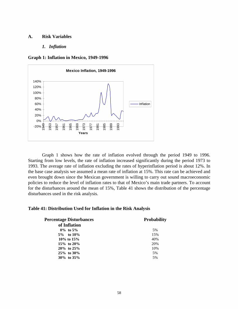
58
A. Risk Variables
1. Inflation
Graph 1: Inflation in Mexico, 1949-1996
Mexico Inflation, 1949-1996
-20%
0%
20%
40%
60%
80%
100%
120%
140%
1949
1953
1957
1961
1965
1969
1973
1977
1981
1985
1989
1993
Years
Inflation
Graph 1 shows how the rate of inflation evolved through the period 1949 to 1996.Starting from low levels, the rate of inflation increased significantly during the period 1973 to1993. The average rate of inflation excluding the rates of hyperinflation period is about 12%. Inthe base case analysis we assumed a mean rate of inflation at 15%. This rate can be achieved andeven brought down since the Mexican government is willing to carry out sound macroeconomicpolicies to reduce the level of inflation rates to that of Mexico’s main trade partners. To accountfor the disturbances around the mean of 15%, Table 41 shows the distribution of the percentagedisturbances used in the risk analysis.
Table 41: Distribution Used for Inflation in the Risk Analysis
Percentage Disturbances of Inflation
Probability
0% to 5% 5%5% to 10% 15%10% to 15% 40%15% to 20% 20%20% to 25% 10%25% to 30% 5%30% to 35% 5%

59
2. Investment Cost Overrun
In the base case, a contingency cost of 11% of total investment has already been takeninto account. In spite of this cost contingency provision, it is likely that the actual level of costoverruns exceeds the amount of that provision. To account for the dispersion of the costoverruns, we use a step distribution in the model of the risk analysis. That distribution rangesfrom 0% to 30% of total investment cost with the expected value equal to the contingency cost of11%. Table 42 shows the distribution used for cost overruns in the risk analysis.
Table 42: Distribution Used for Cost Overruns in the Risk Analysis
Percentage of TotalInvestment
Probability
0%-10% 50%10%-20% 40%20%-30% 10%
3. Real Fuel Cost
The sensitivity analysis shows that changes in real fuel cost impact both financial andeconomic results. The real oil prices show very little long term trend. The short run real pricesfluctuate around that trend. In the base case analysis, we assume that the cost of fuel used forelectricity generation is affected by the world price of oil. Graph 2 shows the real U.S importedoil price, the trend and the deviation from the trend for the period 1976-1996.
Graph 2: Real U.S Imported Oil Price, Trend, and Deviation from Trend, 1976-1996
REAL U.S. IMPORTED OIL PRICES, TREND, DEVIATION FROM TREND, 1973-1996
-10.00
-5.00
0.00
5.00
10.00
15.00
20.00
1973
1975
1977
1979
1981
1983
1985
1987
1989
1991
1993
1995
Year
$/B
arre
l
Real Oil Price
CalculatedDeviation from Trend
The probability distribution of the percentage deviations between the trend values and theactual values, is given in Table 43. In the risk analysis, we use that distribution to account for theannual disturbances of the real fuel prices.

60
Table 43: Percentage Disturbances of Real Oil Price
Percentage Disturbancesof Real Oil Price
Probability
-40% to -30% 4%-30% to -20% 13%-20% to -10% 25%-10% to 0% 17%0% to 10% 8%
10% to 20% 8%20% to 30% 13%30% to 40% 13%
4. Real Exchange Rate
From 1954 to 1996, the real exchange rate expressed in 1990 new pesos averages 2.72pesos per dollar. The average growth of the real exchange rate in the same period is 0.4%, whichis illustrated by the trend line of Graph 3. In the base case we assume a growth of 0% for the realexchange rate.
In addition to the growth rate, the real exchange rate moves up and down in the shortterm. In the case of Mexico these movements have been frequent and large since 1974. Suchmovements will have an impact on this project due to its reliance on oil as a major input. Thesemovements are illustrated by the error terms in Graph 3 below. The average of these error termsis zero.

61
Graph 3: Real Exchange Rate, Trend, and Deviations from Trend, Mexico 1954-1996
Real Exchange Rate, Trend and Deviations from Trend, Mexico 1954-1996
-0.50
0.00
0.50
1.00
1.50
2.00
2.50
3.00
3.50
4.00
1954
1958
1962
1966
1970
1974
1978
1982
1986
1990
1994
Years
Pes
os/
$ Real Exchange Rate
Deviations from Trend
Trend (Real Exchange Rate)
To capture the variation of the real exchange rate, we construct a distribution of theannual disturbances of the real exchange rate. The errors have a mean of 0% and a standarddeviation of 35.5%.
For the purposes of the risk analysis it is the level of the average real exchange rate thatthe project experiences over its life that has the most significant impact on the project outcome.Given the high volatility of the year to year change in the real exchange rate, most of these annualchanges cancel each other out. If the annual changes in the real exchange rate have a mean ofzero and a standard deviation of 35.5% then the movement of the mean real exchange rateaveraged over the life of the project will have a mean of zero and a standard deviation of 7.75%.It is this normal distribution that is used in the risk analysis of this project
5. Technical loss Reduction
The benefits from loss reduction account for 50% of total financial benefits. Thisimportant share requires good estimates of the level of loss reduction. To account for thevariability of these estimates, we use a normal distribution with a range from -15% to 15% of thebase case level in the model of the risk analysis.
6. Changes in Estimate of Maximum Willingness to Pay
In the base case, the changes in the estimate of the maximum willingness to pay is 0%.We used a normal distribution to account for the uncertainty about the actual value of themaximum willingness to pay with a range of –15% to 15%.

62
7. Changes in Estimate of Cost of Outage
In the base case, the changes in the estimate of the cost of outage is 0% . We used anormal distribution with a range of –15% to 15% to account for the uncertainty about the actualvalue of this cost. The probability distributions of all variables used in the risk analysis aresummarized in Table 44.
Table 44: Table of Risk variables.
Risk Variable Base Case Mean Value
ProbabilityDistribution
Range Value Probability
1. Inflation Rate 15% Step 0% to 5%5% to 10%
10% to 15%15% to 20%20% to 25%25% to 30%30% to 35%
5%15%40%20%10%5%5%
2. InvestmentCost overrunfactor
11% Step 0% - 10%10%-20%20%-30%
50%40%10%
3. AnnualPercentageChange in RealOil Price
0% Step -40% to -30%-30% to –20%-20% to –10%
-10% to 0%0% to 10%
10% to 20%20% to 30%30% to 40%
4%13%25%17%8%8%
13%13%
4. PercentageChange inAverage RealExchange Rate
0% Normal -23% to 23% Mean =0Standard
Deviation=7.75%
5. Technical LossFactor
0% Normal (-15) to (15%) Mean =0%Standard
Deviation= 5%
6. PercentageChanges inEstimate ofMaximumWillingness topay
0% Normal -15% to 15% Mean =0%Standard
Deviation= 5%
7. Changes inEstimates of Costof Outage
0% Normal -15% to 15% Mean =0%Standard
Deviation= 5%

63
B. Risk Analysis Results
Table 45 summarizes the results of the risk analysis. Consumers gain the most, about3,114 billion pesos, from this project followed by the government, 648 billion pesos, and labor,86 billion pesos. The economic, total investment, and the equity net present values are 3,842,1,576, and 1,957 billion pesos respectively with almost zero probability of any loss.
Table 45: Risk analysis results(Billion of Pesos)
NPVEquity
NPV TotalInvestment
NPVEconomic
Government Labor Consumers
ExpectedValue
1,957 1,576 3,842 648 86 3,114
Probabilityof negativevalue
0.21% 0.06% 0.18% 0.14% 0.17% 0.29%
The following graph illustrates the cumulative distribution for the equity and economic NPVs ofthe project.
Cumulative Comparison
.000
.250
.500
.750
1.000
0 1,250 2,500 3,750 5,000
EconomicTotal Invesment
Billion Pesos

64
VII. CONCLUSION
The results of the risk analysis show that all present values calculated have almost zeroprobability of negative return pointing to a highly attractive project. The results obtained in therisk analysis are close to the values calculated in the base case analysis. In the risk analysis, theeconomic, total investment, and the equity net present values are 1.3%, 2.6%, and 2.3% lowerthan their corresponding values of the base case analysis.
The transmission component of the CFE rehabilitation and expansion program appears tobe a highly attractive project from both financial and economic perspectives. If the project isimplemented successfully, it is expected to add net wealth of at least 3,894 billion pesos to theMexican economy.

65
ANNEX A: ENVIRONMENTAL IMPACTS OF THE TRANSMISSION PROJECT
The potential environmental impacts for a transmission project include electromagneticradiation, noise, erosion and change in land use. A few studies have related electromagneticradiation from transmission lines to cancer in humans, but there is still very little evidence tosubstantiate this conclusion. The erosion from temporary or permanent earthworks reduces soillevels and affects agriculture and terrestrial ecosystems. The right-of-way land for thetransmission line could displace households or limit land use for agriculture and other productiveuses.58
The assessment of the environmental impacts include broadly two steps. The first stepconsists of identifying and screening the impacts, and the second step deals with thequantification and valuation of the impacts.
1. Impact Identification and Screening
This first step consists of identifying all relevant environmental stressors and thenselecting the most important ones for economic evaluation. In general, four environmentalstressors can be identified in a transmission project. These are: electromagnetic radiation, Noise,Erosion, and Land Use. The first two put a burden on air while the erosion and land use put aburden on land.
The following table summarizes the taxonomy for evaluating potential impacts of theenvironmental stressors in the transmission project.
Table 46: Taxonomy for Evaluating Potential Impacts of the Environmental Stressors inthe Transmission Project
Stressor HumanHealth
Human Welfare EnvironmentalResources
GlobalSystem
Morbidity Materials Aesth-etics
ResourceUse
Social/Cultural
Biodiversity/EndangeredSpecies
TerrestrialEcosystem
Potential Emission/ Burden to AirGasesElectromagneticRadiation
ü
Noise ü ü ü ü
Potential Emission/ Burden to LandHazardousChemicalsErosion ü üLand Use ü ü ü ü ü ü ü ü
58 Economic Evaluation of Environmental Impacts, Asian Development Bank, p.62

66
2. Impacts Quantification and Valuation
The impacts of the stressors have to be quantified in physical and monetary units.Whenever market prices of the impacts are not available, the analyst has to use data from primaryor secondary valuation methods.
A. Electromagnetic Radiation
Since there is no evidence to substantiate the conclusion that relates diseases such ascancer in humans to electromagnetic radiation, we did not evaluate the economic impact of thisstressor in this project. Should evidence relating human cancer to electromagnetic radiationemerge, the following table provides partial data to evaluate the environmental impact of thatstressor. The data will have to be adjusted to reflect costs of cancer effects in Mexico.
Summary Of Selected Monetary Values for Cancer Effects59 (1990 $)
Dollars per NonfatalCancer Case
Dollars per FatalCancer Case
Average Dollars forAll Cancer Casea
Low $102,000 $1.7 million $0.9 millionCentral $204,000 $3.3 million $1.7 millionHigh $408,000 $6.6 million $3.4 milliona Based on the average 5-year cancer survival rate of 51% in the United States
B. Noise
This stressor affects human health and welfare, and the environmental resources. Theimpacts of noise on health and human welfare can be minimized or internalized whereas theimpact on Biodiversity and endangered species can be high. No valuation of the impact of noisewas made in this appraisal because of the lack of relevant data.
C. Erosion
The impacts of the soil erosion are unknown in this project because data are insufficientto assess the erosion rate or the nutrient loss due to the transmission project.
D. Land Use
The land use has impacts on human health, human welfare, and environmental resources.There are little impacts on human health due to the land used in a transmission project. Theimpacts on human welfare, especially the changes in visual aesthetic can be substantial althoughtheir effects can be mitigated by landscaping the corridor of the transmission lines. The socialimpacts such as the displacement of residential dwellings are more difficult to mitigate.
59 Economic Evaluation of Environmental Impacts, Asian Development Bank, p 200-- Source: Rowe et Al. (1994)

67
In the present study we restricted the evaluation of the impacts of the land use to thesocial burden and we used difference between the willingness to pay (WTP) for the land in thevicinity of the transmission lines and the WTP for other lands away from the project area toproxy the environmental costs. However, since no data collected through surveys or other studieswere readily available, we estimated the environmental costs to be 20% of the averagewillingness to pay for agricultural, industrial, recreational and residential lands in Mexico.
In conclusion, the damages of the land use could be large, but some impacts aremitigated rendering the remaining effects over the life of the transmission project uncertain orsmall.
68
REFERENCES
Commission Federal de Electricidad(CFE), “Proyecto especial para la rehabilitacion ymodernizacion de unidades generadoras del area de generacion thermoelectrica deCFE, 1989, Programa No.1 Unidades de 300/350 MW,” 1989.
Commission Federal de Electricidad(CFE), “Proyecto de inversiones en el area de transmission,”1989.
Gutierez, Luis E., “Economic Analysis of A Power Investment Program,” World Bank, January1991.
Harberger, Arnold and Glenn Jenkins, Manual “Program on Investment Appraisal andManagement," Harvard Institute for International Development, 1997.
Jenkins, Glenn P. and El-Hifnawi, Mostafa B., “Economic Parameters for the Appraisal ofInvestment Projects:Bangladesh, Indonesia, and the Philippines,” Report for theEconomics and Development Center, Asia Development Bank, 1994.
Taylor, Lester D. (1975), “The Demand for Electricity: A Survey,” Bell Journal Of Economics,6(1), pp.74-110.
Lim, Henry B.F., “Cost-Benefit Analysis For Peak-Load Pricing And Load Management,” 1979,Ph.D. Dissertation, University of Chicago. Appendix C, “Capital Stock And TheDemand For Electricity By Households And Industry” and D, “Evaluation OfPrevious Studies On The Demand For Electricity.”
Westley, Glenn D., “New Directions in Econometric Modelling of Energy Demand,"InterAmerican Development Bank/ John Hopkins University Press, 1992.
World Bank Report (14298-IN) for Orissa state of India, 1966.
World Bank, "Sectoral Electricity Demand in Mexico: A Forecasting Model," Report (9304-ME),January 14, 1991.
Marsh, W.D., “Economics of Electric Utility Power Generation,” Clarendon Press. Oxford, 1980.
Price Waterhouse, “Doing Business in Mexico,” 1991 Information Guide.
Economic Evaluation of Environmental Impacts, Asian Development Bank.
Max Steinberg, Theodore Smith, Economy Loading of Power Plants and Electric Systems.