Evaluation and Redesign of Beit Dajan Water Distribution Network

EVALUATION AND REDESIGN OF A COMPANY’S DISTRIBUTION
NETWORK
A Record of Study
by
SERGIO ARMANDO BURGOS FUENTES
Submitted to the Office of Graduate Studies of Texas A&M University
in partial fulfillment of the requirements for the degree of
DOCTOR OF ENGINEERING
August 2004
Major Subject: Engineering College of Engineering

EVALUATION AND REDESIGN OF A COMPANY’S DISTRIBUTION
NETWORK
A Record of Study
by
SERGIO ARMANDO BURGOS FUENTES
Approved as to style and content by:
________________________________
Donald R. Smith Chair of Advisory Committee
________________________________
Mark L. Spearman Head, Industrial Engineering
________________________________
Sila Çetinkaya Member
________________________________ Guy L. Curry
Member
______________________________ Lorraine Eden
Member
________________________________
Ben Albrecht, Multiquip, Inc. Internship Supervisor
________________________________
Karen Butler-Purry Coordinator, College of Engineering
August 2004

iii
ABSTRACT
Evaluation and Redesign of a Company’s Distribution Network. (August 2004)
Sergio Armando Burgos Fuentes,
B.S., Universidad de las Américas-Puebla, México;
M.S., Texas A&M University
Chair of Advisory Committee: Dr. Donald R. Smith
The current Record of Study presents the qualitative and quantitative analysis of a
company’s network of distribution centers with the purpose of determining the
convenience and the feasibility to reconfigure such a network. The study was performed
with a multidisciplinary team of people within and outside of the organization. The
distribution network was modeled in various forms and different solutions were obtained
as new information was gathered from questionnaires, from observation and from the
company’s databases. Finally a recommendation was formulated to modify the current
configuration of the distribution network and the feasibility to implement the suggested
solution in practice was evaluated.

iv
ACKNOWLEDGEMENTS
This is a great opportunity for me not only to acknowledge but also to thank the people
that helped me in one way or another to succeed during the past few years that I have
been pursuing the D. Eng. degree.
First, I would like to thank Dr. Don Smith for teaching me so much during the years I
have studied under his guidance, then for giving me the opportunity to serve the
Industrial Engineering Department as his assistant in the Distance Learning Program,
and finally for serving as chair of my doctoral committee and always being a source of
support and friendship.
I would like to thank my professors, Dr. Sila Çetinkaya, Dr. Lorraine Eden and Dr. Guy
Curry who were the best professors I had during my graduate studies at Texas A&M and
then continued to teach me invaluable lessons in their advisory capacity as members of
my advisory committee.
Also, I would like to acknowledge and thank Mr. Ben Albrecht for trusting me and
giving me the opportunity to collaborate with Multiquip on the elaboration of this
project. Working under his supervision was truly an enjoyable learning experience.
Finally, I would like to thank and acknowledge CONACYT (Consejo Nacional de
Ciencia y Tecnologia) for funding my studies at Texas A&M University.

v
TABLE OF CONTENTS
Page
ABSTRACT .............................................................................................................. iii
ACKNOWLEDGEMENTS ...................................................................................... iv
TABLE OF CONTENTS .......................................................................................... v
LIST OF FIGURES................................................................................................... vii
LIST OF TABLES .................................................................................................... viii
INTRODUCTION..................................................................................................... 1
COMPETITIVE ENVIRONMENT ASSESSMENT ............................................... 3
Survey............................................................................................................ 3 Other Sources of Information........................................................................ 10 Conclusions ................................................................................................... 13
GRAVITY CENTER ANALYSIS............................................................................ 15
ANALYSIS OF CURRENT DISTRIBUTION PRACTICES.................................. 20
ANALYSIS OF POTENTIAL LOCATIONS .......................................................... 28
Selection of Potential Locations.................................................................... 28 Model Formulations with Set of Potential Locations.................................... 30 Sensitivity of Solution................................................................................... 39 Size of Distribution Centers .......................................................................... 41
FEASIBILITY OF EASTERN DISTRIBUTION CENTER .................................... 43
RECOMMENDATIONS AND CONCLUSIONS.................................................... 45
REFERENCES.......................................................................................................... 48
APPENDIX A QUESTIONNAIRE FOR MANUFACTURERS AND DISTRIBUTORS OF CONSTRUCTION AND POWER EQUIPMENT................................................................................. 49

vi
Page
APPENDIX B WAREHOUSE LOCATION AND TYPE FROM QUESTIONNAIRES ..................................................................... 53
APPENDIX C RESPONSES TO REMAINING QUESTIONS FROM QUESTIONNAIRES ..................................................................... 54
APPENDIX D DATA SUMMARY FOR DISTRIBUTION CENTER QUOTATION ................................................................................ 56
APPENDIX E FINAL OBJECTIVES DOCUMENT............................................. 57
APPENDIX F INTERNSHIP SUPERVISOR’S FINAL REPORT ....................... 62
VITA ......................................................................................................................... 64
vii
LIST OF FIGURES
FIGURE Page
1 Centers of Gravity for One, Two and Three Geographic Zones ................... 19
2 Current Configuration of Distribution Centers and Service Areas ............... 21
3 Suggested Configuration of Current Distribution Centers and Service Areas................................................................................................. 25
4 Potential Locations ........................................................................................ 29
5 Final Recommended Configuration with Three Distribution Centers........................................................................................................... 37

viii
LIST OF TABLES
TABLE Page
1 Number of DCs by Location from Questionnaires (Including Multiquip) ................................................................................. 5
2 Number of DCs by Type from Questionnaires (Not Including Multiquip) .......................................................................... 5
3 Some Locations Chosen by Competitors That Did Not Respond to the Questionnaire ............................................................................................. 6
4 Number of Warehouses by Location from Questionnaires ........................ 7
5 Size of Distribution Centers from WERC’s Study..................................... 10
6 Number of Distribution Centers from WERC’s Study .............................. 11
7 Type of Distribution Centers from WERC’s Study ................................... 12
8 Example of Demand Aggregation (First Phase) ........................................ 16
9 Example of Demand Aggregation (Second Phase) .................................... 17
10 Aggregation of Products into Nine Classes................................................ 22
11 Changes from Current to Recommended Configuration of Current Distribution Centers ................................................................................... 25
12 Summary of Results for Current Practices and Alternatives...................... 27
13 Potential Locations ..................................................................................... 29
14 Summary Results of Potential Locations Model without Service Level Constraint ......................................................................................... 32 15 Summary Results of Potential Locations Model with Service Level Constraint ......................................................................................... 33

ix
TABLE Page
16 Summary Results of Potential Locations Model with Service Level Constraint and Fixed Costs3 ............................................................ 35
17 Distribution of Product Outflows by Source Distribution Center.............. 38
18 Distribution of Product Outflows by Product Family ................................ 38
19 Process to Estimate Distribution Center Capacities ................................... 42
20 Recommended Distribution Center Capacities .......................................... 42

1
INTRODUCTION
Multiquip, Inc. is a manufacturer and distributor of light and medium-sized construction
equipment with its headquarters located in Carson, California. The company purchases
components for its manufacturing facilities and finished goods for distribution in the
USA on a global basis. Currently the firm’s manufacturing and distribution centers are
located as follows:
1. Atlanta, Georgia – Distribution center.
2. Boise, Idaho – Manufacturing facility and distribution center.
3. Carson, California – Headquarters and distribution center.
4. Montreal, Canada – Distribution center.
5. Newark, New Jersey – Distribution center.
6. Peosta, Iowa – Distribution center.
7. Puebla, Mexico – Manufacturing facility.
Ninety percent of the company’s shipments are concentrated in the US, and one-half of
the international shipments go to Canada and Mexico. Domestically the states of
California, Texas, Florida and New York concentrate about 40% of the total demand.
The distribution network mentioned above was the subject of study during the course of
the year-long internship that is being reported here. Due to the high volume of domestic
sales a decision was made during the kickoff meetings to narrow the scope of the study
to US demand only.
__________
This Record of Study follows the format and style of the Journal of Business Logistics.

2
The work was done under the supervision of Mr. Ben Albrecht, General Manager of
Operations at Multiquip, and it involved working in collaboration with a cross-functional
team within the organization and even outside the organization with people in real-estate
companies, in competing businesses, in third-party logistics providers, in professional
associations and other organizations.
The first part of the project started on June 2003 and was concluded at the end of
December 2003. Among other activities, this part of the project involved trips to the
manufacturing facility in Puebla, Mexico and the headquarters and distribution center in
Carson, California to get acquainted with the company and to observe its operations.
Also an assessment of the company’s competitive environment was performed, the
logistics and operational practices at the distribution centers were analyzed, and data
were gathered and analyzed on-site and from a distance via the company’s SAP R/3
system.
The second part of the project, which concludes with the presentation of this report and
the final examination began on January 2004 and mainly involved the modeling of the
company’s distribution network with the use of optimization software that is available
through the Industrial Engineering Department at Texas A&M University, presenting the
results to Multiquip’s upper managers and assessing the feasibility of the solution
recommended.
It has been agreed with Multiquip, Inc. that proprietary information including demand,
cost and sales figures among other types of information would not be disclosed in the
elaboration of this report. Hence the analyses and results are given in general form, that
is, without revealing information sensitive to Multiquip, Inc.

3
COMPETITIVE ENVIRONMENT ASSESSMENT
Survey
In times of growth in the economy of an industry it is frequent for its individual
members to expand its supplying capabilities in order to satisfy the also increasing
demand from its customers. Naturally, when the economy faces a downturn companies
focus their attention on the reduction of costs as the satisfaction of demand in itself stops
being a constraint and attaining efficiency in its satisfaction becomes the main concern.
Along with the national economy, the construction industry in the U.S. found itself in
such a downturn at the beginning of this century and Multiquip, being a supplier of
construction equipment had a decrease in sales as did all of its direct competitors, and
thus reducing costs on the supply side of the equation became a priority.
The first step to assess the efficiency of Multiquip’s distribution network and the
potential for savings in distribution costs by changing its configuration was to perform
an analysis of the company’s competitive environment and the way in which competitors
operate.
Due to the wide variety of products that are distributed by Multiquip, its number of
competitors is also wide and many of them are direct competitors only in a few product
lines. Therefore, a list of the most significant competitors was put together, and nineteen
companies became the subject of the study in the initial phase of the project.
The study was carried out by sending the nineteen chosen firms a questionnaire about
their distribution organization, their delivery commitment, their freight policy and after-
sale support. The participation of the firms that filled out the questionnaire which is
included on Appendix A was obtained by assuring them that their identity would not be
disclosed at any time. Thus, the results of the study will be provided without revealing

4
the name of any of the companies associated to the different responses. Out of the
nineteen companies, five filled out and returned the questionnaires, for a response rate of
26%. However, only one in these five filled it out completely and with detailed
responses. The rest of them failed to provide complete or suitable answers to every one
of the questions in the questionnaire.
Information about ten of the companies that did not return the questionnaires was
gathered from their websites, journals and other web-based publications. Therefore,
some degree of information was obtained for fifteen companies, that is, 79% of the total,
and no relevant information was obtained for four of the nineteen companies that
represent the remaining 21% of the sample.
The answers provided by the participating companies indicated that they have a number
of warehousing facilities that ranges between one and six. Also, three of the five
indicated that they have third party warehouses, and only two of them said that they also
have customers used as distribution centers as is shown on Appendix B.
If we include the information provided by Multiquip in the results, these yield a
preference for the state of California to place warehousing facilities, as eight of the
twenty four warehouses are located in that state. The states of Iowa, New Jersey, South
Carolina, Wisconsin and also Canada ranked second with a total of two facilities each. A
summary of these results is shown below in Table 1.
Similarly, a preference for company owned facilities was indicated by the companies’
responses. Multiquip’s information on this subject will be omitted, but nine of the fifteen
warehouses from the competitor’s questionnaires belong to this category (53%), while
five of them are third party owned (29%), and only three of them are customers used as
distribution centers (18%). Table 2 below provides a summary of these results.

5
TABLE 1
Number of DCs by Location from Questionnaires (Including Multiquip) Location CA IA NJ SC WI CAN CO GA ID IL KS TX Total
Maquoketa 1 1 Atlanta 1 1 Boise 1 1
Carson 1 1 Cerritos 1 1
Columbia 1 1 Columbia 1 1 Corona 1 1 Fremont 1 1
Ft. Worth 1 1 Germantown 1 1
Itasca 1 1 Montreal 1 1 Newark 1 1 Ontario 1 1 Olathe 1 1 Peosta 1 1
Pleasant Grove 1 1
Riverside 1 1 Rock Hill 1 1
Sacramento 1 1 Swedesboro 1 1
Torrance 1 1 Waukesha 1 1
Total 8 2 2 2 2 2 1 1 1 1 1 1 24
TABLE 2 Number of DCs by Type from Questionnaires (Not including Multiquip)
Type CA SC WI CAN CO IA IL KS NJ TX Total Third Party 1 1 1 1 1 5
Owned 3 2 2 1 1 9 Customer 2 1 3
Total 6 2 2 1 1 1 1 1 1 1 17

6
Partial information about eight of the other competitors was gathered from their
resources online, and other internet-based resources. This information includes the
location of some of their distribution centers, but the type of facility it is unknown, as
well as the total number of distribution centers that these companies have. Table 3 below
shows the locations found to be used by other competitors to place their warehouses.
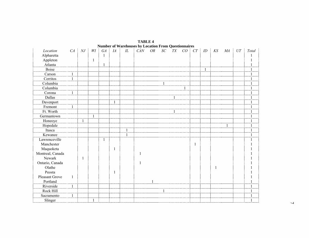
Finally, Table 4 combines the information gathered from questionnaires with the
information obtained from other resources and shows the preferred locations for
warehousing facilities by city and state.
TABLE 3
Some Locations Chosen by Competitors That Did Not Respond to the Questionnaire City State
1 Torrance CA 2 Manchester CT 3 Alpharetta GA 4 Lawrenceville GA 5 Davenport IA 6 Kewanee IL 7 Wood Dale IL 8 Hopedale MA 9 Swedesboro NJ
10 Honeoye NJ 11 Portland OR 12 Troy OR 13 Dallas TX 14 West Jordan UT 15 Appleton WI 16 Slinger WI
7
TABLE 4 Number of Warehouses by Location From Questionnaires
Location CA NJ WI GA IA IL CAN OR SC TX CO CT ID KS MA UT TotalAlpharetta 1 1Appleton 1 1Atlanta 1 1Boise 1 1
Carson 1 1 Cerritos 1 1
Columbia 1 1 Columbia 1 1 Corona 1 1Dallas 1 1
Davenport 1 1Fremont 1 1
Ft. Worth 1 1Germantown 1 1
Honeoye 1 1Hopedale 1 1
Itasca 1 1 Kewanee 1 1
Lawrenceville 1 1Manchester 1 1Maquoketa 1 1
Montreal, Canada 1 1Newark 1 1
Ontario, Canada 1 1Olathe 1 1 Peosta 1 1
Pleasant Grove 1 1Portland 1 1Riverside 1 1Rock Hill 1 1
Sacramento 1 1Slinger 1 1

8
TABLE 4 Continued Location CA NJ WI GA IA IL CAN OR SC TX CO CT ID KS MA UT Total
Swedesboro 2 2Torrance 2 2
Troy 1 1 Waukesha 1 1
West Jordan 1 1 Wood Dale 1 1
Total 9 4 4 3 3 3 2 2 2 2 1 1 1 1 1 1 40
9
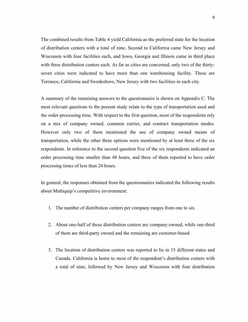
The combined results from Table 4 yield California as the preferred state for the location
of distribution centers with a total of nine. Second to California came New Jersey and
Wisconsin with four facilities each, and Iowa, Georgia and Illinois came in third place
with three distribution centers each. As far as cities are concerned, only two of the thirty-
seven cities were indicated to have more than one warehousing facility. These are
Torrance, California and Swedesboro, New Jersey with two facilities in each city.
A summary of the remaining answers to the questionnaire is shown on Appendix C. The
most relevant questions to the present study relate to the type of transportation used and
the order-processing time. With respect to the first question, most of the respondents rely
on a mix of company owned, common carrier, and contract transportation modes.
However only two of them mentioned the use of company owned means of
transportation, while the other three options were mentioned by at least three of the six
respondents. In reference to the second question five of the six respondents indicated an
order processing time smaller than 48 hours, and three of them reported to have order
processing times of less than 24 hours.
In general, the responses obtained from the questionnaires indicated the following results
about Multiquip’s competitive environment:
1. The number of distribution centers per company ranges from one to six.
2. About one-half of these distribution centers are company-owned, while one-third
of them are third-party owned and the remaining are customer-based.
3. The location of distribution centers was reported to lie in 15 different states and
Canada. California is home to most of the respondent’s distribution centers with
a total of nine, followed by New Jersey and Wisconsin with four distribution

10
centers each; Georgia, Iowa and Illinois with three each and the remaining states
and Canada with one or two distribution centers only.
4. Most respondents utilize different transportation strategies, but few of them
utilize company-owned transportation.
Other Sources of Information
The sample responses that were obtained from the previous survey provide an indication
of the prevalent practices in warehousing within Multiquip’s competitive environment.
However we also looked at other references on warehousing trends and we found a study
called “Facility Trends 2001 – 2003”1 by The Warehousing Education and Research
Council (WERC). In this study they looked at the size and composition of warehousing
networks and compare their findings to the results of similar studies they have performed
in the past. WERC’s study includes the responses of about 140 firms that hold
membership in the council. The majority of these firms is in manufacturing (40%), and
wholesaling (37%), with the rest of them in sectors such as retailing, government,
utilities and others.
In terms of warehousing space, WERC’s study found that the size of most warehouses in
the US is smaller than 500,000 square feet as is shown on Table 5.
TABLE 5
Size of Distribution Centers from WERC’s Study Warehousing Space (square feet) Percentage of Respondents
0 – 100,000 37% 100,000 – 500,000 31%
500,000 – 1,000,000 21% 1,000,000 – 3,000,000 6%
3,000,000 - 5%

11
Perhaps the most significant finding of WERC’s study is the fact that the respondents’
overall number of facilities in their network of distribution centers is decreasing. From
2001 to 2003, the size of distribution networks has decreased in number by 4.4% as is
reproduced from WERC’s study on Table 6.
TABLE 6
Number of Distribution Centers from WERC’s Study Industry 2001 2002 2003 Change in 2 years
Electronics / Computing 5.4 5.1 4.7 -14.2% Pharmaceutical / Medical 2.7 2.5 2.7 0% Grocery / Food / Beverage 12.5 12.7 12.1 -3.1% Industrial / Office products 3.4 3.5 3.6 +5.3%
Consumer goods 4.7 4.0 4.1 -15.5% OVERALL 5.5 5.3 5.2 -4.4%
* Number expected
According to the analysis, the overall size in warehouse networks is expected to decrease
in all sectors. However the industrial sector does show an increasing trend, but they
argue that it may be due to the small size of that sector’s sample (n=16) and their
relatively small network size of 3.5 warehouses. The overall decline in the number of
distribution centers is attributed to the slowdown of the economy, which has forced
companies in all industries to become more efficient and do the same tasks with fewer
resources.
According to WERC, larger and medium sized companies are most likely to have
reduced the size of their distribution network during 2002. However, they say, the size of
newly built distribution centers is getting bigger. In other words, the trend is for
distribution networks to become smaller in number, but the size of the distribution
centers is increasing. The factors mentioned to explain this increasing size of facilities
include mergers and acquisitions, and “the fact that warehouses are being asked to do
more value added services (VAS). In addition to traditional warehousing functions, DC’s

12
are now being called upon as facilities where light manufacturing takes place, customer
center call centers are placed and corporate transportation headquarters are located. As
the trend for VAS continues, it is probable that size of DCs will continue to increase.”
The respondents who have modified the configuration of their distribution networks
indicated that the main reason for such changes was sales-related (i.e. inventory turns),
as well as overall inventory conditions. Other reasons included the need for increased
labor flexibility, acquisitions and mergers, product sourcing changes, customs and duty
and transportation costs.
With respect to the type of distribution centers mostly utilized, WERC classifies them as full-line, limited-line, or overflow. Also, they differentiate between private, public or contract facilities; this classification gives them nine possible warehouse combinations. For the purposes followed in our study we are only interested to know the preferences in terms of private, public and contract warehousing. Accordingly, the mix of distribution centers with respect to their contractual agreements is shown on Table 7.
TABLE 7 Type of Distribution Centers from WERC’s Study
Type of DC 1998 2002 Private 65% 73% Public 27% 14%
Contract 8% 13% In general terms, three observations can be made. First, private distribution centers are
by far the most prevalent, and their usage is increasing. Second, the trend in public
warehousing usage is going down, and third, contract warehouses represent a very small
part of all warehouses being used, but the trend is for them to become more common.

13
Conclusions
The results of the survey with Multiquip’s list of nineteen competitors yielded limited
results in terms of the response rate. Even though response rates for similar studies
seldom go beyond forty percent, the small response rate coupled with the small sample
size yielded results that couldn’t be considered statistically representative of the industry
average.
However, some insights could be drawn. First, the number of distribution centers in the
competitor’s distribution networks seems to be smaller than that of Multiquip. Second, it
is known that at least one of the competitors in the study has joined the trend reported by
WERC’s study, namely, they have reduced their number of warehouses and increased its
size with respect to what they had in the past. Third, three of the top six preferred states
for warehouse location in the study coincide with states where Multiquip runs its
distribution centers, that is, California, New Jersey and Georgia.
In terms of transportation, only two of the respondents indicated that they utilize
company owned resources, while four of the five indicated that they use common carrier
transportation as one of their transportation means. In second place came the use of
contract transportation with three competitors mentioning it as one of their transportation
means. However, the difference between these three choices of transportation is too
small to draw significant conclusions.
On the freight question, it is clear that all competitors view it as a marketing and sales
tool. They offer reduced freight charges to stimulate the placement of larger orders or to
close a deal, so any strategy to relocate a distribution center should pay close attention to
the selection of sites with good availability of freight carriers and low freight rates.

14
Finally, the trends reported by WERC’s study suggest that Multiquip’s number of
distribution centers is too large in comparison with industry standards, and it could be
reduced thus forcing the remaining warehouses to be more efficient than currently.

15
GRAVITY CENTER ANALYSIS
The results obtained from the Competitive Environment Assessment supported the
opinions of Multiquip managers that a location analysis should be conducted to
determine the most advantageous configuration of the firm’s distribution network.
In order to obtain an initial solution to the warehouse location problem, a gravity center
analysis was performed. The gravity center approach is an analytic tool that finds the
single location that will minimize the transportation distance when considering all the
shipments to the different customers. Mathematically, this problem solves for the
minimum distance between two points in the Euclidean distance case.
The term “gravity center” arises for the following reason: If we were to place a map of
the area in which the distribution center is to be located on a heavy piece of cardboard
and weights proportional to demands were placed at the locations of demand points, then
the gravity center solution would be the point on the map at which the entire system
would balance2.
The mathematical solution to the gravity center problem is given at the location:
∑
∑
=
== k
nn
k
nnn
D
xDx
1
1' , and ∑
∑
=
== k
nn
k
nnn
D
yDy
1
1' (1)
where xn and yn represent the coordinate location of either a market or supply source n,
and Dn represents the quantity to be shipped between facility and market or supply
source n.

16
The demand data considered in this analysis covered the period of January, 2002 to
August, 2003. Such information was downloaded from Multiquip’s SAP R/3 system and
it included the name and zip code of each customer as well as the dollar amount that was
demanded during those 20 months. Coordinate locations for supply and demand points
were given by the longitude and latitude of the different locations’ zip codes which were
available for the execution of this project from a commercial database. Given the great
number of Multiquip customers or demand points, they were aggregated in two stages:
1. First, “shipped to” customers were aggregated into clusters according to the
three-digit zip code, thus reducing its number from 10,307 individual customers
to 846 customer zones. So for example, all customers in zip code areas starting
with the three digits 989 were put together into one customer zone as shown on
Table 8.
TABLE 8 Example of Demand Aggregation (First Phase)
Location Zip Code
Gross Sales @ cost (01/02 to
08/03)
New Customer Zone
Gross Sales @ cost (01/02 to
08/03) 98901 $ 3,712 98909 $ 174 98944 $ 275 98902 $ 400 98926 $ 760 98903 $ 3,489
TOTAL $ 8,810 989 $ 8,810 * These numbers do not represent real sales figures
2. It has been documented in the literature that aggregating large amounts of data
achieves a significant reduction in variability, and forecast demand is much more
accurate at the aggregated level. Furthermore, the aggregation of data into about
150 to 200 points usually results in no more than about 1% error in estimation of
total transportation costs3. Therefore, the previous 846 customer zones were
further aggregated into 141 demand clusters by geographical proximity, with all

17
of them having about the same demand level. In other words, assuming that the
total domestic demand for the 20 months mentioned above equaled $11,635,650,
then dividing this amount by 141, it would yield clusters of about $82,522. Table
9 shows an example of this aggregation stage.
TABLE 9
Example of Demand Aggregation (Second Phase)
Customer Zone Domestic Gross Sales @ cost (20
months)
New Demand Cluster
Domestic Gross Sales @ cost (20
months) 984 $ 20,852 985 $ 3,557 986 $ 5,686 988 $ 7,256 989 $ 10,810 990 $ 6 991 $ 130 992 $ 25,385 993 $ 2 270 994 $ 48
TOTAL $ 76,000 142 * These numbers do not represent real sales figures
With the demand and location information aggregated in this fashion, a local gravity
center was obtained for each of the 141 demand clusters. As it was explained before, the
gravity centers were obtained in the form of a coordinate pair, one coordinate indicating
the location’s longitude and the other one its latitude, and seldom did these coordinates
coincide with an actual city. Thus the distance from the gravity center to each of the
individual locations in the demand clusters was calculated and the closest city was then
chosen to be the cluster’s gravity center.
Finally a “global” gravity center analysis was performed in three scenarios that follow
along with its results.
18
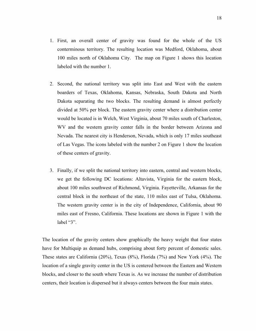
1. First, an overall center of gravity was found for the whole of the US
conterminous territory. The resulting location was Medford, Oklahoma, about
100 miles north of Oklahoma City. The map on Figure 1 shows this location
labeled with the number 1.
2. Second, the national territory was split into East and West with the eastern
boarders of Texas, Oklahoma, Kansas, Nebraska, South Dakota and North
Dakota separating the two blocks. The resulting demand is almost perfectly
divided at 50% per block. The eastern gravity center where a distribution center
would be located is in Welch, West Virginia, about 70 miles south of Charleston,
WV and the western gravity center falls in the border between Arizona and
Nevada. The nearest city is Henderson, Nevada, which is only 17 miles southeast
of Las Vegas. The icons labeled with the number 2 on Figure 1 show the location
of these centers of gravity.
3. Finally, if we split the national territory into eastern, central and western blocks,
we get the following DC locations: Altavista, Virginia for the eastern block,
about 100 miles southwest of Richmond, Virginia. Fayetteville, Arkansas for the
central block in the northeast of the state, 110 miles east of Tulsa, Oklahoma.
The western gravity center is in the city of Independence, California, about 90
miles east of Fresno, California. These locations are shown in Figure 1 with the
label “3”.
The location of the gravity centers show graphically the heavy weight that four states
have for Multiquip as demand hubs, comprising about forty percent of domestic sales.
These states are California (20%), Texas (8%), Florida (7%) and New York (4%). The
location of a single gravity center in the US is centered between the Eastern and Western
blocks, and closer to the south where Texas is. As we increase the number of distribution
centers, their location is dispersed but it always centers between the four main states.

19
FIGURE 1
Centers of Gravity for One, Two and Three Geographic Zones
1122
22 3333
33

20
ANALYSIS OF CURRENT DISTRIBUTION PRACTICES
The core business of Multiquip is the distribution of construction equipment, some of
which it manufactures and some of which it purchases, but the core business activity is
distribution. Therefore the main cost drivers are related to inbound and outbound
transportation. On the supply side Multiquip receives finished product and parts from
about 700 suppliers while on the demand side it ships product to more than 10,000
customers, hence the weight of outbound transportation costs is far greater than that of
inbound transportation. Having that in mind, the next step in the analysis of Multiquip’s
distribution network was to study the company’s current distribution practices and the
associated outbound distribution costs associated to them.
The current policies have assigned a number of states to each of the five distribution
centers. In other words, each state’s demand should be supplied from only one
distribution center. In practice this is followed as closely as possible, but sometimes it is
necessary to violate this policy due to inventory fluctuations, unexpected demand
changes or other special circumstances. An analysis was performed to compare the
distribution practices under the current policies to the optimal distribution practices
without changing the number or location of the current distribution centers.
More specifically, the distribution network was modeled mathematically to minimize the
total shipping cost from the existing distribution centers in Carson, Atlanta, Peosta,
Boise and Newark to the different demand clusters. These distribution centers and their
current service areas are identified graphically on Figure 2.

21
FIGURE 2
Current Configuration of Distribution Centers and Service Areas
11
22
33 55
44
22
Definitely, the most important piece of information for such formulation is the set of
freight rates for transportation from distribution center i to demand location j of product
k. The i demand locations are given by 137 of the 141 demand clusters obtained before.
The remaining four clusters were ignored because they are located outside of the
conterminous United States, so these clusters include customers in Alaska, Hawaii, and
Guam.
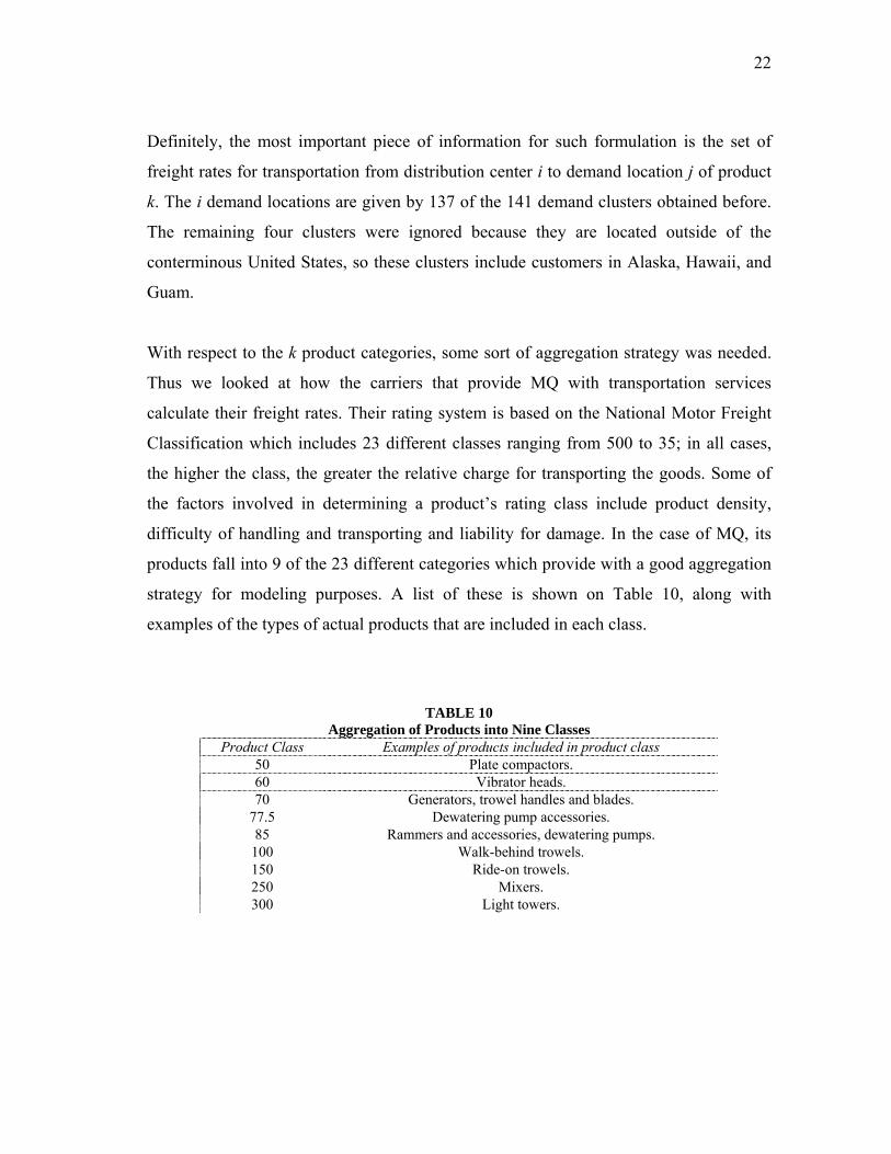
With respect to the k product categories, some sort of aggregation strategy was needed.
Thus we looked at how the carriers that provide MQ with transportation services
calculate their freight rates. Their rating system is based on the National Motor Freight
Classification which includes 23 different classes ranging from 500 to 35; in all cases,
the higher the class, the greater the relative charge for transporting the goods. Some of
the factors involved in determining a product’s rating class include product density,
difficulty of handling and transporting and liability for damage. In the case of MQ, its
products fall into 9 of the 23 different categories which provide with a good aggregation
strategy for modeling purposes. A list of these is shown on Table 10, along with
examples of the types of actual products that are included in each class.
TABLE 10
Aggregation of Products into Nine Classes Product Class Examples of products included in product class
50 Plate compactors. 60 Vibrator heads. 70 Generators, trowel handles and blades.
77.5 Dewatering pump accessories. 85 Rammers and accessories, dewatering pumps. 100 Walk-behind trowels. 150 Ride-on trowels. 250 Mixers. 300 Light towers.

23
Freight rates were then obtained from Southern Motor Carrier’s Complete Zip Auditing
and Rating (CzarLite) engine. This software offers a market-based price list derived
from studies of LTL pricing on a regional and interregional basis and therefore provides
with very good estimates of actual freight rates for individual carriers. For the purposes
of this analysis an average shipment was considered to range between 17,500 and 25,000
pounds. The use of freight rates for shipments in that range effectively overestimates the
shipping cost of many orders and underestimates that of a few, but on average the total
error in shipping cost estimation is relatively small. Consequently, the freight rates
downloaded represented the transportation cost of such average shipment for each
combination of distribution centers and customer zones. Finally, the demand data were
transformed from dollar value to weight in pounds by considering the average weight of
a product in each of the nine aggregation categories.
Mathematically, the solution to minimize the transportation cost of Multiquip’s current
distribution network can be modeled as an assignment problem. A simplified version of
the Warehouse Location Problem was formulated as is shown below:
FORMULATION 1
Indices
i demand clusters i = 1,…,137
j distribution center j = 1,…,5
k product families k = 1,…,9
Parameters
cijk cost to transport 1 unit of product k from distribution center j to demand cluster i
dik annual pounds of product k required by demand cluster i
Variables
xijk fraction of demand dik supplied from distribution center j

24
Minimize (2) ∑∑∑= = =
=137
1
5
1
9
1i j kijkikijk xdcz
Subject to i = 1,…,137; k = 1,…,9 (3) ,15
1∑=
=j
ijkx
0≥ijkx i = 1,…,137; j = 1,…,5; k = 1,…,9 (4)
The linear nature of this mathematical formulation does not allow us to consider the
economies of scale associated to the transport of larger shipments. Hence the solution to
the model is equivalent to comparing the cost to satisfy the demand at a customer zone
from each of the five possible distribution centers and choosing the one with the lowest
cost and multiplying it by its associated demand. Then, repeating the process for all of
the 137 demand clusters in each of the 9 product categories and adding up the 1233
subtotals would result in the same solution as the linear programming formulation does.
The data were downloaded from the company’s SAP R/3 system and then organized in
Microsoft’s Excel and Access. The model was formulated in AMPL© and solved with
CPLEX 7.1©. The solution resulted in savings of 9.5% with respect to the current
practice which was shown graphically on Figure 2. In contrast, the alternative solution to
the current configuration is represented on Figure 3 below. The main result of this
analysis is the benefit that could be achieved by reassigning the states of Texas, Ohio,
Indiana, Missouri, Michigan and Oklahoma that are currently served from Peosta to be
served by Atlanta instead. The resulting savings in outbound freight costs are broken
down by reassigned state on Table 11 below.
Although Multiquip’s main objective in conducting this study was to minimize costs it
should not be done at the expense of customer service. Thus a measure of customer
service was defined as the proportion of demand that can be supplied in one day, which
occurs when the demand cluster is within 600 miles of its servicing distribution center.

25
FIGURE 3
Suggested Configuration of Current Distribution Centers and Service Areas
11
22
33 55
44
TABLE 11
Changes from Current to Recommended Configuration of Current Distribution Centers
State Original Servicing DC Suggested Servicing DC % Annual Savings in Outbound Freight Cost
Texas Peosta Atlanta 5.57 Ohio Peosta Atlanta 1.59
Indiana Peosta Atlanta 0.75 Missouri Peosta Atlanta 0.65 Michigan Peosta Atlanta 0.56 Oklahoma Peosta Atlanta 0.37
Total Savings 9.49%
26
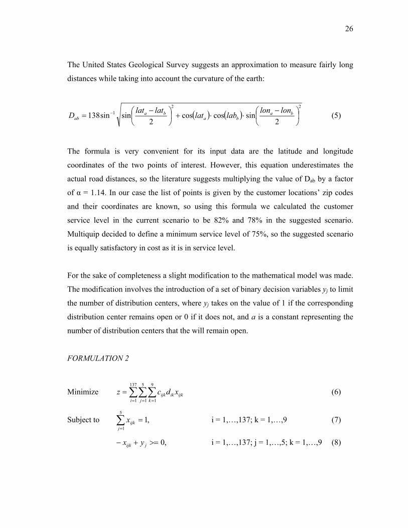
The United States Geological Survey suggests an approximation to measure fairly long
distances while taking into account the curvature of the earth:
( ) ( )22
1
2sincoscos
2sinsin138 ⎟
⎠⎞
⎜⎝⎛ −
⋅⋅+⎟⎠⎞
⎜⎝⎛ −
= − baba
baab
lonlonlablatlatlatD (5)
The formula is very convenient for its input data are the latitude and longitude
coordinates of the two points of interest. However, this equation underestimates the
actual road distances, so the literature suggests multiplying the value of Dab by a factor
of α = 1.14. In our case the list of points is given by the customer locations’ zip codes
and their coordinates are known, so using this formula we calculated the customer
service level in the current scenario to be 82% and 78% in the suggested scenario.
Multiquip decided to define a minimum service level of 75%, so the suggested scenario
is equally satisfactory in cost as it is in service level.
For the sake of completeness a slight modification to the mathematical model was made.
The modification involves the introduction of a set of binary decision variables yj to limit
the number of distribution centers, where yj takes on the value of 1 if the corresponding
distribution center remains open or 0 if it does not, and a is a constant representing the
number of distribution centers that the will remain open.
FORMULATION 2
Minimize (6) ∑∑∑= = =
=137
1
5
1
9
1i j kijkikijk xdcz
Subject to i = 1,…,137; k = 1,…,9 (7) ,15
1∑=
=j
ijkx
,0>=+− jijk yx i = 1,…,137; j = 1,…,5; k = 1,…,9 (8)
27
∑=
=5
1jj ay (9)
0≥ijkx i = 1,…,137; j = 1,…,5; k = 1,…,9 (10)
{ }1,0∈jy j= 1,…,5 (11)
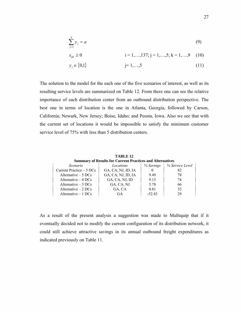
The solution to the model for the each one of the five scenarios of interest, as well as its
resulting service levels are summarized on Table 12. From there one can see the relative
importance of each distribution center from an outbound distribution perspective. The
best one in terms of location is the one in Atlanta, Georgia, followed by Carson,
California; Newark, New Jersey; Boise, Idaho; and Peosta, Iowa. Also we see that with
the current set of locations it would be impossible to satisfy the minimum customer
service level of 75% with less than 5 distribution centers.
TABLE 12
Summary of Results for Current Practices and Alternatives Scenario Locations % Savings % Service Level
Current Practice – 5 DCs GA, CA, NJ, ID, IA 0 82 Alternative – 5 DCs GA, CA, NJ, ID, IA 9.49 78 Alternative – 4 DCs GA, CA, NJ, ID 9.13 74 Alternative – 3 DCs GA, CA, NJ 5.78 66 Alternative – 2 DCs GA, CA 0.81 52 Alternative – 1 DCs GA -52.43 29
As a result of the present analysis a suggestion was made to Multiquip that if it
eventually decided not to modify the current configuration of its distribution network, it
could still achieve attractive savings in its annual outbound freight expenditures as
indicated previously on Table 11.

28
ANALYSIS OF POTENTIAL LOCATIONS
The results that were obtained during the previous stages of the analysis provided us
with enough preliminary information that reinforced our initial thoughts that a
reconfiguration of the distribution network was advisable and feasible. Furthermore, to
this point we had already gathered a substantial amount of information and a simplified
formulation of the Warehouse Location problem had already proven to be a viable
option to model Multiquip’s distribution network.
Selection of Potential Locations
The next step in the study was to develop a list of potential locations to establish new
distribution centers or to consolidate existing ones. To begin with, we looked at the
current literature on the subject to find the ratings of different cities for the location of
new distribution facilities. Such a list was compiled by Expansion Management4, and it
ranks cities according to criteria such as rail road availability, taxes and fees, interstate
highways, and other categories. The list of cities listed in this article provides the reader
with very few surprises as most of the locations are among the largest cities in the
country. In other words one would only need to write a list of the main cities in each
state and it would probably look very similar to the list in the referred article. Therefore
it was decided to use the list only as a reference, but we needed to develop a list of
potential locations in accordance to the company’s specifics.
The solution to obtain a suitable list of locations was to divide the US conterminous
territory into a number of zones with just about the same demand level and then to
determine the center of gravity for each of these zones. Also the six locations resulting
from the gravity center analysis were included in our list of potential sites. The full list
of gravity centers found, which would serve as potential locations is given next on Table
13 and Figure 4 contains a map depicting its locations.

29
TABLE 13
Potential Locations Number Zip Code City State Number Zip Code City State
1 03103 Manchester NH 17 63501 Kirksville MO 2 06902 Stamford CT 18 71203 Monroe LA 3 12777 Monticello NY +19 74103 Tulsa OK
*4 17111 Harrisburg PA +20 74631 Blackwell OK *5 20018 Washington DC 21 74820 Ada OK +6 23909 Farmville VA 22 77449 Huntsville TX +7 24801 Princeton WV 23 78028 Kerrville TX 8 27705 Durham NC 24 82602 Casper WY
*9 29301 Spartanburg SC 25 84501 Price UT *10 31206 Macon GA 26 85541 Payson AZ 11 32301 Tallahassee FL +27 89077 Henderson NV 12 33876 Sebring FL *28 92505 Riverside CA
*13 37228 Nashville TN 29 93204 Avenal CA *14 43215 Columbus OH +30 93720 Fresno CA 15 49224 Albion MI 31 95691 West Sacramento CA
*16 55906 Rochester MN 32 98901 Yakima WA * Location included in Expansion Management’s list of top logistics metros + Location obtained from Gravity Center Analysis
FIGURE 4 Potential Locations
22
11
33
4455
6677
88
991010
1111
1212
1313
1414
15151616
1717
1818
19192020
2121
22222323
2424
2525
2626
27272828
2929
3030
3131
3232
30
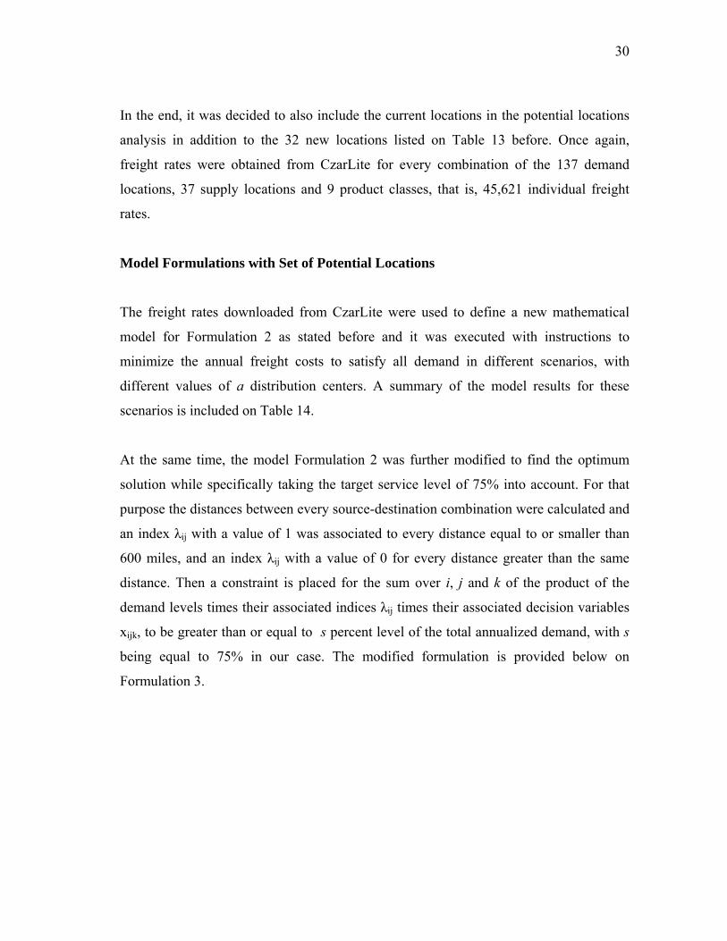
In the end, it was decided to also include the current locations in the potential locations
analysis in addition to the 32 new locations listed on Table 13 before. Once again,
freight rates were obtained from CzarLite for every combination of the 137 demand
locations, 37 supply locations and 9 product classes, that is, 45,621 individual freight
rates.
Model Formulations with Set of Potential Locations
The freight rates downloaded from CzarLite were used to define a new mathematical
model for Formulation 2 as stated before and it was executed with instructions to
minimize the annual freight costs to satisfy all demand in different scenarios, with
different values of a distribution centers. A summary of the model results for these
scenarios is included on Table 14.
At the same time, the model Formulation 2 was further modified to find the optimum
solution while specifically taking the target service level of 75% into account. For that
purpose the distances between every source-destination combination were calculated and
an index λij with a value of 1 was associated to every distance equal to or smaller than
600 miles, and an index λij with a value of 0 for every distance greater than the same
distance. Then a constraint is placed for the sum over i, j and k of the product of the
demand levels times their associated indices λij times their associated decision variables
xijk, to be greater than or equal to s percent level of the total annualized demand, with s
being equal to 75% in our case. The modified formulation is provided below on
Formulation 3.

31
FORMULATION 3
Minimize (12) ∑∑∑= = =
137
1
5
1
9
1i j kijkikijk xdc
Subject to i = 1,…,137; k = 1,…,9 (13) ,15
1∑=
=j
ijkx
,0>=+− jijk yx i = 1,…,137; j = 1,…,5; k = 1,…,9 (14)
∑∑∑= = =
≥137
1
5
1
9
1i j kijkijkij sDxdλ (15)
∑=
=5
1jj ay (16)
0≥ijkx i = 1,…,137; j = 1,…,5; k = 1,…,9 (17)
{ }1,0∈jy j= 1,…,5 (18)
The results for the execution of this model with different values of a for the number of
distribution centers are summarized on Table 15.
In general, the solutions to the formulation without the 600-mile constraint tend to show
a preference for one location in Nashville, TN, and one or two in California and the East
Coast. In fact, we know that California is the single most important market for
Multiquip, but the solutions call for over 70% of the customer orders being served from
distribution centers in Nashville and the East Coast. The main drawback to the solution
of the model in these scenarios is the significant reduction in service level, with only the
5-facilities scenario satisfying the 75% minimum requirement.
When the service level constraint is introduced into the formulation, the solution to the
scenario with five facilities is identical to that of the previous model without the distance
constraint. However there is no solution to the model with only one or two distribution

32
centers. Therefore we can conclude that the minimum number of distribution facilities
for MQ to satisfy its demand with 75% service level constraint is three.
In particular, the scenario with five distribution centers splits the service area of the West
Coast into a northern and a southern region, and the East Coast into a southern, a central
and a northern section, with Nashville as its main distribution center, covering almost
50% of all demand assigned to it for both models. The solution to distance-constrained
scenario with four facilities is almost identical, with the exception that the West Coast is
all assigned to a unique distribution facility in southern California. Finally, the
constrained scenario with three facilities is interesting because it suggests a location in
Tulsa, as opposed to the corresponding unconstrained model which suggested location in
Nashville. In both instances of the two-facility scenario the West Coast is still assigned
to a location in southern California, and the East Coast is serviced from North Carolina.
TABLE 14
Summary Results of Potential Locations Model without Service Level Constraint Scenario Chosen Locations % of Demand % Savings % Service Level
Riverside, CA 16 West Sacramento, CA 12
Stamford, CT 15 Sebring, FL 10
5 DCs
Nashville, TN 47
22 77
Riverside, CA 16 West Sacramento, CA 12
Durham, NC 33 4 DCs
Nashville, TN 38
18 71
Riverside, CA 28 Durham, NC 33 3 DCs
Nashville, TN 38 13 70
Riverside, CA 28 2 DCs Nashville, TN 72 5 53
1 DC Nashville, TN 100 -49 29

33
TABLE 15
Summary Results of Potential Locations Model with Service Level Constraint Scenario Chosen Locations % of Demand % Savings % Service Level
Riverside, CA 16 West Sacramento, CA 12
Stamford, CT 15 Sebring, FL 10
5 DCs
Nashville, TN 47
22 77
Riverside, CA 32 Stamford, CT 16 Sebring, FL 9 4 DCs
Nashville, TN 43
13 76
Riverside, CA 28 Durham, NC 49 3 DCs Tulsa, OK 24
6 77
2 DCs There is no feasible solution 1 DC There is no feasible solution
Having obtained the results summarized on Table 15, it was decided to further increase
the amount of information embedded in the modeling efforts. Second to acquisition and
outbound freight costs, Multiquip’s bill is affected by lease and labor costs. The first of
these costs are fixed in nature, but the second are not as the number of people may vary
in proportion to sales volume. For the purpose of this project it was decided to handle
labor costs as fixed because the number of people required to work at a distribution
center does not normally vary, and any requirements for labor additional to the normal
demand is covered by working overtime.
Labor rates were obtained from the Bureau of Labor Statistics, which is part of the U.S.
Department of Labor. The Bureau’s internet portal provides information as recent as
2002 about wages by area and occupation and it further opens it up by state. In our case,
the Standard Occupational Classification System (SOC) provides average hourly wages
for transportation and material moving occupations, and more specifically for “First-
Line Supervisory/Managers of Transportation and Material-Moving Machine and
Vehicle Operators” under the SOC code number 53-1031. In the states considered in our
modeling efforts as potential locations for new distribution centers, the average hourly
34
salaries for workers in this category range from $18.68 in Utah to $26.42 in the state of
Washington.
Average rental rates for warehousing space are not as readily available as labor rates are.
Therefore the acquisition of estimates for this cost driver was made in coordination with
a large real estate company that is headquartered in California. They conducted a survey
of the areas of our interest to determine general market conditions and average rental
rates for each one of the potential locations considered in this study. The results of our
work in this area ranged from a minimum of $3.17 per square foot per year in Tennessee
to $5.81 in Connecticut.
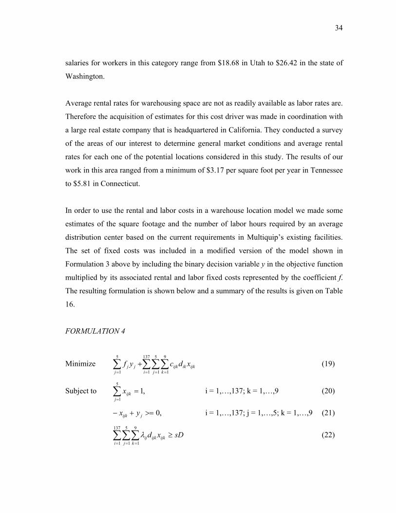
In order to use the rental and labor costs in a warehouse location model we made some
estimates of the square footage and the number of labor hours required by an average
distribution center based on the current requirements in Multiquip’s existing facilities.
The set of fixed costs was included in a modified version of the model shown in
Formulation 3 above by including the binary decision variable y in the objective function
multiplied by its associated rental and labor fixed costs represented by the coefficient f.
The resulting formulation is shown below and a summary of the results is given on Table
16.
FORMULATION 4
Minimize (19) ∑∑∑∑= = ==
+137
1
5
1
9
1
5
1 i j kijkikijk
jjj xdcyf
Subject to i = 1,…,137; k = 1,…,9 (20) ,15
1∑=
=j
ijkx
,0>=+− jijk yx i = 1,…,137; j = 1,…,5; k = 1,…,9 (21)
∑∑∑= = =
≥137
1
5
1
9
1i j kijkijkij sDxdλ (22)

35
∑=
=5
1jj ay (23)
0≥ijkx i = 1,…,137; j = 1,…,5; k = 1,…,9 (24)
{ }1,0∈jy j= 1,…,5 (25)
TABLE 16
Summary Results of Potential Locations Model with Service Level Constraint and Fixed Costs
Scenario Chosen Locations % of Demand % Freight Cost Savings % Service Level
Riverside, CA 28 Durham, NC 25 Sebring, FL 9
Nashville, TN 38 5 DCs
12 78
Riverside, CA 28 Durham, NC 25 Sebring, FL 9 4 DCs
Nashville, TN 38
12 78
Riverside, CA 28 Durham, NC 49 3 DCs Tulsa, OK 24
6 77
2 DCs There is no feasible solution 1 DC There is no feasible solution
The results obtained for the fixed-costs scenario are very similar to the non-fixed-costs
scenario, except for one thing: the introduction of fixed costs into the formulation shows
the sub-optimality of having five distribution centers to supply the company’s domestic
demand.
The solution to this point comes down to having a minimum of three distribution centers
and a maximum of four. In the four-facility scenario one of the distribution centers must
be placed in California and it will supply the demand of the West Coast which as
mentioned before concentrates about 20% of total demand in California. A second
distribution center to supply the demand from the central states should be placed in

36
Tennessee and the East Coast is split in two sections: the first one is located in Florida
and serves only the distribution in that state and the second one remains in North
Carolina.
When it comes to the three-facility scenario the configuration changes in two ways:
First, the distribution center to supply the demand in the central region shifts to the West,
from Tennessee to Oklahoma; and second, the East coast is served by only one section.
Even though there is a six percent differential in freight shipping costs between the two
options in favor of the 4-facility scenario, when fixed costs are included the difference
between both solutions comes down to three percent. When this small economic benefit
is weighed against the logistical complication of operating an additional distribution
center practically devoted to supplying the demand of just one state, the scale leans over
to the three-distribution center scenario.
Finally, the suggested reconfiguration of Multiquip’s distribution network is the three
distribution center solution that was mentioned before with annual savings in freight
shipping costs of six percent. The map on Figure 5 shows the location of the three
distribution centers and their corresponding service areas. It is quite interesting to note
the fact that the final suggested configuration turned out to be quite similar to the
“rough-cut” solution yielded by the three-gravity center analysis previously noted on
Figure 1. Once again the explanation is given by the heavy weight that the states of
California, Texas, New York and Florida have due to their high demand levels.
Tables 17 and 18 provide detailed descriptions of the percent outflows from different
perspectives. Table 17 shows the distribution of outflows traveling from each
distribution center to its destination state. There we can see that by placing the East
Coast distribution center in North Carolina we are putting it halfway through the two
major demand centers in the zone which are New York and Florida and right on the state

37
that ranks third in demand, which intuitively makes sense. Similarly, the central zone is
heavily weighted in Texas and so its location in the zone is very close to it. The Eastern
location from a state standpoint is very straightforward as 60% of the zone’s demand is
from California.
FIGURE 5
Final Recommended Configuration with Three Distribution Centers
11 2233

38
TABLE 17
Distribution of Product Outflows by Source Distribution Center
From NC Total Outflow: 49%
From OK Total Outflow: 24%
From CA Total Outflow: 28%
Outflows by destination
Outflows by Pounds of Product
Outflows by destination
Outflows by Pounds of Product
Outflows by destination
Outflows by Pounds of Product
To: Flow Product Flow To: Flow Product Flow To: Flow Product Flow FL 17.5% 50 8.9% TX 37.1% 50 5.4% CA 60.5% 50 9.7% NY 10.6% 60 0.1% CO 11.4% 60 0.0% AZ 15.7% 60 0.1% NC 6.6% 70 16.7% MO 9.7% 70 22.2% NV 7.2% 70 19.7% PA 6.1% 77.5 0.7% MN 5.6% 77.5 0.1% UT 6.1% 77.5 0.3% OH 5.9% 85 18.3% NM 5.5% 85 20.2% WA 4.9% 85 25.9% GA 5.1% 100 9.3% AR 5.2% 100 11.9% OR 3.5% 100 4.5% VA 4.4% 150 3.3% OK 4.6% 150 3.3% ID 2.1% 150 2.1% CT 4.1% 250 42.1% LA 4.5% 250 35.2% 250 35.5% TN 4.1% 300 0.7% IA 3.1% 300 1.6% 300 2.2% MD 4.0% MS 2.6% NJ 4.0% KS 2.5% IN 3.6% NE 2.5% IL 3.6% SD 2.5% MI 3.5% MT 1.4% AL 3.5% WY 1.3% SC 3.3% ND 0.5% KY 2.7% MA 2.2% WI 1.6% NH 1.5% ME 1.1% WV 1.0% DE 0.0% RI 0.0%
TABLE 18
Distribution of Product Outflows by Product Family Product Family Distribution
Center 50 60 70 77.5 85 100 150 250 300 California 32% 43% 29% 18% 34% 15% 20% 25% 47%
North Carolina 53% 47% 43% 74% 43% 53% 54% 53% 25% Oklahoma 15% 10% 28% 8% 23% 33% 26% 21% 29%
Total 100% 100% 100% 100% 100% 100% 100% 100% 100%

39
The distribution center-percent flows in terms of weight are also broken down by
product family on Table 17. On average those percentages should also reflect the
composition of inventories per facility, if not in quantity of product at least in density or
floor space usage, and in general they are very similar for all three distribution centers.
We can see that in all three cases products in the 250 family (mixers) will occupy most
of the floor space with at least 35% of the total. In second place products in the 70 and
the 85 product families which represent generators and trowel accessories and rammers
and dewatering pumps respectively, are almost equally represented in all three locations.
Together, product families 70, 85 and 250 represent 75 to 80 percent of the total pounds
shipped out of any distribution center.
A different perspective to look at the composition of product outflows is shown on Table
18. There we can see the how each of the nine product families are distributed across the
three distribution centers. In all but one case the facility in North Carolina ships out most
of each product family with at least 40% of the total. The extreme case is that of
dewatering pumps accessories in product family 77.5, which is shipped out of North
Carolina 74% of the time. The one case where the eastern distribution center does not
dominate product outflows is light towers in product family 300. In this case about half
of the product outflows are shipped out of the distribution center in California and the
other half is almost equally shipped out of the other two facilities.
Sensitivity of Solution
The solution to the model with three distribution centers seems to be very robust, but
still, it was decided to analyze the sensitivity of the solution. Due to the large amount of
variables and constraints it is not simple to draw conclusions from the output that
CPLEX 7.1 © generates with the analysis of sensitivity. However it did allow us to
observe general tendencies, and then different scenarios were be evaluated. A summary
of the results obtained in this scenario analysis follows:
40
The suggested location for an eastern distribution center would shift from North
Carolina to a new location under either one of two scenarios: if the fixed costs (labor
and lease) associated to Durham, North Carolina rose beyond 224%, or if the respective
freight shipping costs rose beyond 18%, the new Eastern location would be Harrisburg,
Virginia. However either of these scenarios would also change the location of the other
two distribution centers from Tulsa, Oklahoma to Macon, Georgia in the central part of
the country and from Riverside, California to Henderson, Nevada on the West Coast.
The scenario would not be attractive anymore from an outbound transportation cost
perspective, as this cost would increase by 5% with respect to the current situation.
However the first scenario is practically impossible to occur, and the second is highly
unlikely, for as it was mentioned before the shipping freight costs utilized downloaded
from CzarLite correspond to cost structures that are representative of the market as
opposed to individuals freight carriers, so an 18% differential seems excessive.
The solution to the West Coast location would easily shift the location of its distribution
center in Riverside, California to the current location of Carson in that state. It would
only take a 0.5% increase in freight shipping cost or a combined 1% increase in labor
and lease costs. Therefore it may seem that the model is very sensitive to changes in cost
for the eastern distribution center, however if we re-run the model by removing
Riverside from the set of potential locations then it follows that Carson becomes the new
model solution. In this case it would take a 12.5% increase in freight shipping costs or a
combined increase of 53% in labor and lease costs to switch the location of the western
location to Fresno, California. It is clear then that either Riverside or Carson is the best
location for a distribution facility on the West Coast. However, freight shipping costs
from Carson would bring the total savings in this area down from 6% to 5%.
In the central region, placing the distribution center in any of the three Oklahoma
locations makes no difference from a cost perspective. In any case, Tulsa should be the

41
selected location due to its better access to highways, and in general because of its better
infrastructure. Therefore the question to ask here would be: In which scenario would the
selected location of a distribution center in the central region stop being in the state of
Oklahoma? The answer to this question is when either shipping freight costs out of all
Oklahoma locations increased beyond 12.5% or when labor and lease costs in
combination increased beyond 48%. In either of these two scenarios the selected location
for a distribution center in the central region would be Monroe, Louisiana. The savings
associated to this scenario would be about four percent of shipping freight costs and the
service level would be 75%. Once again it seems quite unlikely that the cost structures in
Oklahoma would turn out to be so much higher than our estimates, so the location of a
distribution facility in Tulsa, Oklahoma seems quite reasonable.
Size of Distribution Centers
After defining the number and location of distribution centers in the company’s
distribution network, we faced the challenge of determining the right size for each of the
facilities.
In order to estimate the size requirements we decided to utilize inventory turnover ratios
for each product family as suggested by Simchi-Levi3. An inventory turnover ratio ρ is
calculated as the ratio of the total annual flow fk of each product family k through the
distribution center to its corresponding average inventory level ik, that is: kkk if=ρ ,
and therefore kkk fi ρ= . The process to get these estimates is summarized on Table
19.

42
TABLE 19
Process to Estimate Distribution Center Capacities Step Description Source of Information 1 Gather inventory turnover ratios ρk for each product family k. Accounting department.
2 Determine annual flows fjk through each of the j distribution centers and for each product family k.
Solution to model formulation 4 in 3-facility scenario.
3 Determine average inventory levels ijk = fjk/ ρjk in each distribution center for each product family. Steps 1 and 2.
4 Determine average floor space requirement sk of product family k Product specifications
5 Multiply sk by ijk for every k and every j in order to compute total floor space requirements Sjk in each distribution center. Steps 3 and 4
6 Observe stacking levels lk for product family k Stacking strategy
7 Compute tjk, the actual amount of square feet required by product family k in distribution center j as follows: tjk = Sjk / lk.
Steps 5 and 6
8
Compute Tj, the total space required in distribution center j as follows: c∑
jjkt for product family k, where c is an adjustment
factor to account for the maximum inventory level and any space required for aisle space, material handling equipment, etc.
Step 7
Following this procedure with the actual data, we estimated the following capacities for
the company’s distribution centers as shown on Table 20. These capacities represent an
upper bound on the capacity requirements; however they have a number of assumptions
built into the analysis including stability of demand to reflect the historic demand during
2002 and 2003. Even so, these estimates should be very reasonable for the establishment
of the new facilities if it was decided to do so.
TABLE 20
Recommended Distribution Center Capacities Distribution Center Estimated Square Feet Required
North Carolina 51,700 Oklahoma 25,900 California 26,400

43
FEASIBILITY OF EASTERN DISTRIBUTION CENTER
For some time, the company’s decision makers had felt that Multiquip’s distribution
network could be sized down without compromising its service level standards by
identifying the appropriate number and location of its distribution centers. After the
results so far discussed on this document were presented the company’s upper managers
they made the decision to pursue the suggested solution and to redirect the team’s efforts
towards the execution of their decision.
Due to contractual circumstances in the current distribution centers, the schedule to
execute the network’s reconfiguration should start by evaluating the feasibility to
consolidate the eastern facilities currently located in Georgia and New Jersey into one
facility in the state of North Carolina.
The market for contract warehousing in North Carolina had already been assessed in
collaboration with the real estate company mentioned before during the industrial market
research phase to obtain average lease rates. The conclusion was that vacancy in the state
for contract warehousing started to decline during first half of 2003, after it reached its
highest level during the last five years towards the end of 2002. At this moment
warehousing space availability should not be considered a major constraint, and average
asking lease rates in the state for warehouse space are $4.95 per square foot per year.
Moreover, thirty eight available facilities were identified in the cities of Durham,
Raleigh and Charlotte with asking lease rates ranging from $2.00 to $6.25 per square
foot per year.
Contract warehousing is only one of the options available to provide a company with
warehousing space. Due to previously satisfactory experience with public warehousing
as an alternative to lease a facility, an assessment of the feasibility to partner with a third
party logistics provider (3PL) was performed. 3PLs in the state of North Carolina were

44
researched and contacted to inquire on their space availability and their ability to handle
the company’s warehousing needs. A total number of 10 3PLs expressed their interest to
partner with Multiquip and initial quotes were requested from each one of them. In order
to facilitate their task to put together a quote for Multiquip’s business a summary of the
company’s warehousing needs was sent to them. The format sent is included on
Appendix D. Naturally, the form was sent to the 3PLs with all the information filled in,
but the company’s proprietary information is omitted here for obvious reasons. Six of
the ten 3PLs that had originally expressed interest on the project provided us with
proposals that are feasible from an economic and a business standpoint. Their asking
lease rates ranged from $3.00 to $6.60 per square foot per year, and they also provided
quotes for labor, throughput and other measures to allow us to make comparisons.
After reviewing the information gathered on contract and public warehousing in North
Carolina, the feasibility to locate a consolidated distribution center in the state was
confirmed, and upper management decided in favor of the second type of arrangement.
Public warehousing is the most attractive option to Multiquip because it does not tie up
resources in the acquisition of fixed assets, and also it gives the company the flexibility
to terminate the contractual arrangement with the 3PL at any given moment since this
type of arrangements are not fixed on a long term basis. Furthermore, previous
experience with public warehousing has proven to be very efficient for the handling of
Multiquip’s warehousing needs.
A 3PL’s ability to adequately satisfy the needs of a warehousing partner goes far beyond
its availability of space and attractive lease rates. Thus the importance to carefully assess
the fit of both companies cannot be overlooked. This is why it has been recommended
that managers at Multiquip spend enough time visiting the candidate 3PLs in North
Carolina and getting familiar with their facilities, their capabilities and limitations, and
most importantly their people to assess the likelihood of a cultural fit.

45
RECOMMENDATIONS AND CONCLUSIONS
As a result of all the technical and non-technical work and analysis performed on
Multiquip’s competitive environment and current configuration of its distribution
network the following recommendations and conclusions are formulated:
1. Multiquip should have a minimum number of three distribution centers, and a
maximum of four. Having less than two facilities makes it impossible for the
company to satisfy its minimum service level requirements, and having more
than four facilities is not cost effective. Furthermore, a number of three
distribution centers should be the best strategy, because the cost increment with
respect to having four facilities is only 3% of freight shipping, labor and lease
costs, and it makes more sense from a logistics stand point to operate a less
complex network of distribution centers.
2. The demand on the East coast should be supplied from a 50,000 square feet
distribution center located in North Carolina. On the west coast, the distribution
center currently located in Carson, California is adequately located in that city. A
third distribution center with storage capacity of 25,000 square feet should be
placed in the state of Oklahoma to supply the demand in that section of the
country. A graphic description of these locations and the customer zones
associated to them is shown on Figure 6. Similarly, a detailed summary of the
product flows leaving each distribution center is given on Tables 17 and 18.
3. The location of a distribution facility in North Carolina is feasible in either of
these forms of warehousing: contract or public. However preference is expressed
for a public warehousing solution for it allows more flexibility on both partnering
parties and it has proven to be a successful strategy for Multiquip in the past.

46
Also the availability of freight carriers in North Carolina was verified and most
of the carriers that currently work with Multiquip on the east coast were found to
provide their services out of North Carolina.
4. Savings associated with the suggested solution will be in the order of 5% of
outbound freight shipping costs, 30% of lease, labor, utilities and other facilty-
related costs and savings in inventory holding costs that have not been quantified
in this study, but will surely result from the reduction of safety stocks following
the consolidation of the distribution centers.
5. The east coast consolidation should be carried out as a first step in the
reconfiguration of Multiquip’s distribution network. Upon completing this phase
the current business situation should be reassessed in order to validate the
recommendations listed here.
6. Further analysis should be conducted to determine alternative distribution
strategies. For example, the possibility for Multiquip to partner with large
customers to hold small inventories in strategic locations could be explored.
7. Even if Multiquip decided not to pursue the consolidation recommendations
listed on this document, savings in the order of 9% in outbound shipping costs
could be realized by reassigning the demand that is generated in some states to
the current distribution centers as indicated on Table 11 and Figure 4.
It is the author’s opinion that the results and recommendations made to Multiquip during
the course of this project have been useful, and if implemented they could have an
impact in the bottom line of the company through the potential cost savings.

47
It is also important to mention here that this project was a great learning process to the
author, not only because of the technical challenges associated with the solution of
problem, but also because of the challenges associated with determining and obtaining
data and having to work with many different people of different backgrounds, in
different locations and even from different organizations. Working on this project gave
the author exposure to non-technical problems including communications and business
etiquette that are seldom encountered in school projects, and in that sense the objectives
of the internship were accomplished as stated in the Doctor of Engineering brochure:
“(1) to enable the student to demonstrate and enhance his or her abilities and to apply the
knowledge gained from technical training in making a significant contribution of
practice concern to the intern’s employer, and (2) to enable the student to function in a
nonacademic environment and become familiar with the employer’s approach to
problems in addition to traditional approaches of engineering design or analysis”.

48
REFERENCES
1 Wilson, Gary, “Facility Trends 2001-2003” Warehousing Education and Research
Council, (September 2002): pp. 1-12.
2 Nahmias, Steven, Production and Operations Analysis, 4th, Ed. , McGraw Hill, Boston,
Mass. (2001).
3 Simchi-Levi, David, Kaminsky, Philip and Simchi-Levi, Edith, Designing and
Managing the Supply Chain: Concepts, Strategies and Case Studies, Irwin/McGraw
Hill, Boston, Mass (2000).
4 King, Bill and Keating, Michael, “100 Most Logistics-Friendly Cities in America”
Expansion Management, Vol. 18, No. 9 (2003): pp. 52-64.

49
APPENDIX A
QUESTIONNAIRE FOR MANUFACTURERS AND DISTRIBUTORS OF CONSTRUCTION AND POWER EQUIPMENT
1. This questionnaire is for manufacturers and distributors of construction and
power equipment. The questionnaire solicits information on your business’s distribution organization, delivery commitment, freight policy and after-sale support in the US.
2. The information you provide will be used for an academic project in the
Industrial Engineering department at Texas A&M University and it will be treated confidentially. The information gathered will be shared with all the participating companies who would like to have it, without revealing anyone’s identities.
3. Please return this questionnaire by e-mail or fax, and direct any questions to:
Sergio A. Burgos Doctor of Engineering Student, Texas A&M University E-mail: [email protected] Phone: (979) 777-1139 Fax: (979) 458-1089
4. Please designate an individual from your organization to verify any unclear answers or receive additional information:
Contact Person
Company Name Title
Address City/St/Zip
Phone Fax
Please keep a copy of this questionnaire in the event I need to contact you for clarification. Thanks.

50
APPENDIX A
Continued
I. Distribution Organization
A. How many distribution centers does your organization have?
B. Does your organization use customers as distribution centers (Yes/No)?
C. Please indicate the location of your organization’s distribution centers. Also indicate whether they are company-owned (CO), third party warehouses (3P) or customers used as distribution centers (CUS). City State CO / 3P
/ CUS City State CO / 3P /
CUS 1 26 2 27 3 28 4 29 5 30 6 31 7 32 8 33 9 34 10 35 11 36 12 37 13 38 14 39 15 40 16 41 17 42 18 43 19 44 20 45 21 46 22 47 23 48 24 49 25 50

51
APPENDIX A
Continued
D. Does your organization use common carrier, contract or company-owned transportation? Explain below.
II. Delivery Commitment
A. What is the order processing time for items in stock?
B. What is your organization’s back order policy? Explain below
III. Freight Policy
A. What is your organization’s FOB point? Explain below
B. Is freight used as a marketing or sales tool? Explain below

52
APPENDIX A
Continued
IV. After-Sale Support
A. How is your organization’s after-sale service provided? Is it through company-owned service centers, third-party authorized centers or through the dealer network? Explain below.
B. Provide a description of your organization’s warranty policy
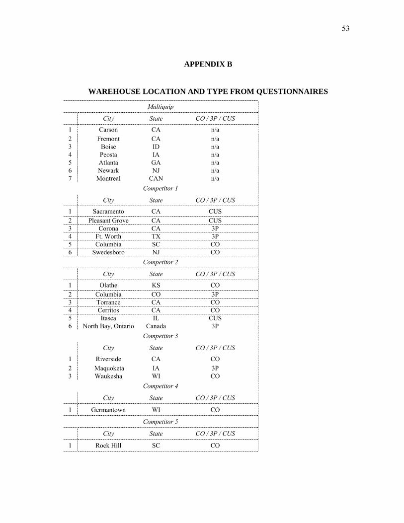
53
APPENDIX B
WAREHOUSE LOCATION AND TYPE FROM QUESTIONNAIRES
Multiquip
City State CO / 3P / CUS
1 Carson CA n/a 2 Fremont CA n/a 3 Boise ID n/a 4 Peosta IA n/a 5 Atlanta GA n/a 6 Newark NJ n/a 7 Montreal CAN n/a
Competitor 1
City State CO / 3P / CUS
1 Sacramento CA CUS 2 Pleasant Grove CA CUS 3 Corona CA 3P 4 Ft. Worth TX 3P 5 Columbia SC CO 6 Swedesboro NJ CO
Competitor 2
City State CO / 3P / CUS
1 Olathe KS CO 2 Columbia CO 3P 3 Torrance CA CO 4 Cerritos CA CO 5 Itasca IL CUS 6 North Bay, Ontario Canada 3P
Competitor 3
City State CO / 3P / CUS
1 Riverside CA CO 2 Maquoketa IA 3P 3 Waukesha WI CO
Competitor 4
City State CO / 3P / CUS
1 Germantown WI CO
Competitor 5
City State CO / 3P / CUS
1 Rock Hill SC CO

54
APPENDIX C
RESPONSES TO REMAINING QUESTIONS FROM QUESTIONNAIRES
Delivery Commitment
Organization Choice of transportation Order
processing time
Backorder policy
Competitor 1 Common carrier 24 hours
If equipment is on backorder, the customer is notified and they are the first to get it when more equipment
comes in
Competitor 2
UPS for parts, common carrier for parts and small equipment, trucking companies for larger
equipment, and company owned transportation for some sales.
Orders placed by 3 p.m. are shipped the
same day 96% of the time
We will inform the customer, and we’ll tell them when we expect the
product to be available. Then we will automatically ship the equipment to
them as soon as it is available.
Competitor 3 Contract transportation and common carrier 1 to 6 days
The customer can choose to have the items placed on backorder status, and
shipped to him when they’re available.
Competitor 4 Company owned and UPS 24 to 24 hours n/a
Competitor 5 Contract transportation and UPS Within 12 hours of order n/a
Competitor 6 Common carrier 48 hours Ship when available. If over 60 days
contact customer to verify order before shipment.
Freight Policy Organization Is Freight used as a marketing tool? FOB point
Competitor 1 Yes. Freight rates vary with order size, customer type, etc. Freight charges are
waived for special promotions.
FOB plant, customer takes ownership when material is shipped.
Competitor 2 Yes, freight varies with order size and other factors. FOB warehouse. Free freight for full truckload orders
Competitor 3 Yes, freight is normally paid for by the company. FOB Plant.
Competitor 4 Yes, freight is used to get customers to order up
Freight is negotiated, but it’s normally paid by company
Competitor 5 Yes FOB delivered on large orders
Competitor 6 Yes, freight is sometimes used to close a deal FOB warehouse

55
APPENDIX C
Continued
After Sale Support
Organization How is your after-sale support provided? Provide a description of your warranty policy
Competitor 1 Dealers for some products and field service personnel
Different for all products. Warranty is determined by manufacturer but we have modified it with
some product lines as a marketing and sales tool
Competitor 2
After-sale service is provided by two company-owned Service Centers, 75
Authorized Service Centers and some of the dealer network.
Most machines carry a standard 1-year warranty, some machines and engines carry 2 years. Parts standard warranty is 90 days, complete engines
carry 1-year warranty.
Competitor 3 Network of company-owned and authorized service centers
30-Day, Warranty. If you're dissatisfied for any reason, just present your proof of purchase for a
full refund within 30 days of purchase. One-Year Free Service contract. Full One-Year Warranty.
We'll repair any defects due to faulty materials or workmanship at no cost to customer — for one
year from the date of purchase Competitor 4 Authorized service centers 2 and 5 year warranty plans
Competitor 5 Over 800 authorized centers worldwide 5 year transferable warranty
Competitor 6 10 authorized service centers Three full years on parts and labor - with engines covered for at least two years by manufacturer

56
APPENDIX D
DATA SUMMARY FOR DISTRIBUTION CENTER QUOTATION
1. Cities/Areas interested in North Carolina: Winston-Salem, Charlotte, Durham,
Greensboro, Chapel Hill, Raleigh, etc.
2. What are the products? Construction Equipment 3. Product specifications/ Inventory breakdown
Maximum Number of SKUs Maximum no. units per pallet Minimum no. units per pallet Pallet size used Racking necessary? Inventory turns per year Maximum footage required Minimum footage required Time period of requirement List special characteristics / requirements::
4. Inbound information Floor loaded Palletized Avg. inbounds/day Avg. inbounds/week Avg. inbounds/month Avg. number of cases per inbound truck: 5. Outbound information Product freight classification No. of orders per day Are orders in pallet quantities? Special characteristics/requirements: 6. Date requirement to begin

57
APPENDIX E
FINAL OBJECTIVES DOCUMENT
On the following four pages, the final objectives document is reproduced as presented
and approved on February 11, 2004.

58
Final Internship Objectives
By
Sergio A. Burgos-Fuentes
Submitted in partial fulfillment of the requirements for the degree of
DOCTOR OF ENGINEERING
February 2004
Major Subject: Engineering
(Industrial Engineering)

59
February 11, 2004
To: Doctor of Engineering Advisory Committee
From: Sergio A. Burgos-Fuentes
Re: Final Internship Objectives
The current document presents a statement of the final objectives for my internship
experience for your review and approval. These objectives are outlined, including the
accomplishments that will ultimately be reported in the Record of Study. My final
internship objectives parallel the objectives stated in my internship proposal without
major variations.
The internship project is taking place at Multiquip, Inc., a manufacturer and distributor
of light and medium-sized construction equipment. Founded in 1972, Multiquip is
currently headquartered in Carson, California, and has five distribution centers
distributed across the nation.
The overall final objective will be to determine the optimum design for MQ’s
distribution network and its logistics practices so as to minimize the company’s annual
costs of supplying its demand, while maintaining an acceptable service level. More
specifically, this objective includes:
Determination of the optimum number, location, and size of distribution centers.
Determination of the geographic areas to be served out of each distribution
center.

60
Determination of the optimum mix of company owned, contract, customer-based
and space-only distribution methods.
Identification of specific facilities in the chosen locations.
Determination of the optimum number of carriers.
Determination of the optimum schedule to implement the suggested solution.
Some specific activities associated with the preliminary objectives include:
Conducting research to determine competitive market requirements.
Collecting and analyzing MQ data to determine shipping patterns and transit time
requirements.
Working with a Real Estate consulting firm to identify specific facilities in
potential sites.
Researching third party logistics providers for fit and value added potential.
Reviewing MQ logistics processes and systems for improvement potential.
Preparing reports, presentations and recommendations to management.
The technical and non-technical aspects of the analysis will be described in detail in the
Record of Study and then discussed and defended in the final examination.
61
Doctor of Engineering Internship Proposal
Final Internship Objectives
By
Sergio Armando Burgos-Fuentes
Approved as to scope and content by: ______________________________ ______________________________ Dr. Donald R. Smith Dr. Guy L. Curry Chair of Advisory Committee Member ______________________________ ______________________________ Dr. Sila Çetinkaya Dr. Lorraine Eden Member Member ______________________________ ______________________________ Mr. Ben Albrecht Karen Butler-Purry Internship Supervisor Coordinator, College of Engineering
February 2004

62
APPENDIX F
INTERNSHIP SUPERVISOR’S FINAL REPORT
The following is the letter written on behalf of Sergio Burgos by his internship
supervisor, Mr. Ben Albrecht.
63

64
VITA
Sergio Armando Burgos Fuentes
Campos Eliseos 2907, Plaza Europa
Puebla, Pue., Mexico, 72540
Mr. Burgos was born on April 14, 1974 in the city of Puebla, Mexico to Mr. Sergio
Armando Burgos-Ochoategui and Mrs. Maria Magdalena Fuentes Guevara. He received
his B.S. degree in industrial engineering from the Universidad de las Americas, Puebla,
Mexico in 1997 and his M.S. degree in industrial engineering from Texas A&M
University in 2001 before entering the Texas A&M University’s Doctor of Engineering
Program in the Fall of 2001. Mr. Burgos also received a Graduate Business Certificate
from Mays Business School at Texas A&M University in 2001. Mr. Burgos specializes
in Distribution and Logistics and his previous industry experience includes working as
an industrial engineering analyst for Tubos de Acero de Mexico, S.A. from July of 1997
to July of 1999.
The preparer of this Record of Study was Sergio Armando Burgos Fuentes.