EVALUATION AND EFFECT OF FRACTURING FLUIDS ON FRACTURE CONDUCTIVITY IN TIGHT GAS...
73
EVALUATION AND EFFECT OF FRACTURING FLUIDS ON FRACTURE CONDUCTIVITY IN TIGHT GAS RESERVOIRS USING DYNAMIC FRACTURE CONDUCTIVITY TEST A Thesis by JUAN CARLOS CORREA CASTRO Submitted to the Office of Graduate Studies of Texas A&M University in partial fulfillment of the requirements for the degree of MASTER OF SCIENCE May 2011 Major Subject: Petroleum Engineering
Transcript of EVALUATION AND EFFECT OF FRACTURING FLUIDS ON FRACTURE CONDUCTIVITY IN TIGHT GAS...

EVALUATION AND EFFECT OF FRACTURING FLUIDS ON FRACTURE
CONDUCTIVITY IN TIGHT GAS RESERVOIRS USING DYNAMIC
FRACTURE CONDUCTIVITY TEST
A Thesis
by
JUAN CARLOS CORREA CASTRO
Submitted to the Office of Graduate Studies of Texas A&M University
in partial fulfillment of the requirements for the degree of
MASTER OF SCIENCE
May 2011
Major Subject: Petroleum Engineering

Evaluation and Effect of Fracturing Fluids on Fracture Conductivity in Tight Gas
Reservoirs Using Dynamic Fracture Conductivity Test
Copyright 2011 Juan Carlos Correa Castro

EVALUATION AND EFFECT OF FRACTURING FLUIDS ON FRACTURE
CONDUCTIVITY IN TIGHT GAS RESERVOIRS USING DYNAMIC
FRACTURE CONDUCTIVITY TEST
A Thesis
by
JUAN CARLOS CORREA CASTRO
Submitted to the Office of Graduate Studies of Texas A&M University
in partial fulfillment of the requirements for the degree of
MASTER OF SCIENCE
Approved by:
Co-Chairs of Committee, Ding Zhu A. Daniel Hill Committee Member, Yuefeng Sun Head of Department, Stephen A. Holditch
May 2011
Major Subject: Petroleum Engineering

iii
ABSTRACT
Evaluation and Effect of Fracturing Fluids on Fracture Conductivity in Tight Gas
Reservoirs Using Dynamic Fracture Conductivity Test. (May 2011)
Juan Carlos Correa Castro, B.S., Universidad Industrial de Santander
Co-Chairs of Advisory Committee: Dr. Ding Zhu Dr. Alfred Daniel Hill
Unconventional gas has become an important resource to help meet our future
energy demands. Although plentiful, it is difficult to produce this resource, when locked
in a massive sedimentary formation. Among all unconventional gas resources, tight gas
sands represent a big fraction and are often characterized by very low porosity and
permeability associated with their producing formations, resulting in extremely low
production rate. The low flow properties and the recovery factors of these sands make
necessary continuous efforts to reduce costs and improve efficiency in all aspects of
drilling, completion and production techniques. Many of the recent improvements have
been in well completions and hydraulic fracturing. Thus, the main goal of a hydraulic
fracture is to create a long, highly conductive fracture to facilitate the gas flow from the
reservoir to the wellbore to obtain commercial production rates. Fracture conductivity
depends on several factors, such as like the damage created by the gel during the
treatment and the gel clean-up after the treatment.
This research is focused on predicting more accurately the fracture conductivity,
the gel damage created in fractures, and the fracture cleanup after a hydraulic fracture

iv
treatment under certain pressure and temperature conditions. Parameters that alter
fracture conductivity, such as polymer concentration, breaker concentration and gas flow
rate, are also examined in this study. A series of experiments, using a procedure of
“dynamical fracture conductivity test”, were carried out. This procedure simulates the
proppant/frac fluid slurries flow into the fractures in a low-permeability rock, as it
occurs in the field, using different combinations of polymer and breaker concentrations
under reservoirs conditions.
The result of this study provides the basis to optimize the fracturing fluids and
the polymer loading at different reservoir conditions, which may result in a clean and
conductive fracture. Success in improving this process will help to decrease capital
expenditures and increase the production in unconventional tight gas reservoirs.

v
DEDICATION
This thesis is dedicated to my family

vi
ACKNOWLEDGEMENTS
I would like to thank my co-chairs, Dr. Ding Zhu and Dr. A. Daniel Hill, for
giving me the opportunity to study under them and pursue my Master of Science degree,
and for their guidance and support throughout the course of this research.
Thanks also goes to Dr. Yuefeng Sun for serving as my committee member. I
would also like to thank John Maldonado, Andres Pieve de La Rosa, Obadare Awoleke
and Jose Romero, for their help and support and for making my time at Texas A&M
University a great experience. Also, I would like to thank the Harold Vance Department
of Petroleum Engineering for giving me the opportunity to pursue my masters degree
and the Research Partnership to Secure Energy for America (RPSEA) corporation for
funding this research project.
Finally, thanks to my mother and father for their encouragement.

vii
TABLE OF CONTENTS
Page
ABSTRACT .............................................................................................................. iii
DEDICATION .......................................................................................................... v
ACKNOWLEDGEMENTS ...................................................................................... vi
TABLE OF CONTENTS .......................................................................................... vii
LIST OF FIGURES ................................................................................................... ix
LIST OF TABLES .................................................................................................... xi
CHAPTER
I INTRODUCTION AND LITERATURE REVIEW ............................ 1
1.1 Hydraulic Fracturing in Tight Gas Reservoirs ............................... 1 1.2 Background and Literature Review ................................................ 3 1.3 Problem Description ....................................................................... 7 1.4 Research Objective ......................................................................... 8 II EXPERIMENTAL SET UP, PROCEDURES, AND CONDITIONS . 10
2.1 Dynamic Fracture Conductivity Test ............................................. 10 2.2 Design of Experiments ................................................................... 11 2.2.1 Generating the Design ........................................................ 12 2.3 Experimental Apparatus Setup ....................................................... 14 2.4 Experimental Procedure ................................................................. 21 2.4.1 Core Sample Preparation .................................................... 22 2.4.2 Assembly of the Fracture Conductivity Cell ...................... 24 2.4.3 Gel and Fracture Fluid Preparation ..................................... 26 2.4.4 Closure Stress Shut-in ......................................................... 29 2.4.5 Fracture Conductivity Procedure ........................................ 30 2.5 Experimental Conditions ................................................................ 34 2.5.1 Rock Sample ....................................................................... 34 2.5.2 Fracturing Fluid Composition ............................................. 34 2.5.3 Proppant Size and Concentration ........................................ 35 2.5.4 Temperature ........................................................................ 35

viii
CHAPTER Page 2.5.5 Nitrogen Gas Flow Rate ..................................................... 35 2.5.6 Closure Stress Loading – Shut-in Time .............................. 37
III EXPERIMENTAL RESULTS AND DISCUSSION ........................... 38 3.1 Experimental Design ...................................................................... 38 3.2 Polymer Loading Effect ................................................................. 40
3.3 Breaker Concentration Effect ......................................................... 46 3.4 Gas Flow Rate Effect ..................................................................... 47
IV CONCLUSIONS AND RECOMMENDATIONS ............................... 49
4.1 Conclusions .................................................................................... 49 4.2 Recommendations .......................................................................... 51
REFERENCES .......................................................................................................... 53
APPENDIX A ........................................................................................................... 56
VITA ......................................................................................................................... 61

ix
LIST OF FIGURES
Page
Figure 1 Unconventional gas production in the United States. ............................ 2 Figure 2 Operations between the parameters. ...................................................... 13 Figure 3 Aliasing generation ................................................................................ 13 Figure 4 Final equations ....................................................................................... 14 Figure 5 Fracture conductivity cell and its parts .................................................. 16 Figure 6 Hydraulic load frame ............................................................................. 18 Figure 7 Pressure transducer port and diaphragms .............................................. 20 Figure 8 Data acquisition system and desktop computer ..................................... 21 Figure 9 Core sample preparation ........................................................................ 23 Figure 10 Fracture conductivity cell setup ............................................................. 25 Figure 11 Schematic representation of fracture conductivity experiment ............. 28 Figure 12 Schematic representation of conductivity measure test ......................... 33 Figure 13 Comparison between experiments at 30 lb/1000gal and 10 lb/1000gal
of polymer loading.…………………………………………………… 41 Figure 14 Cake formed by proppant and residue gel ............................................. 42 Figure 15 Fracture conductivity measurement ....................................................... 43 Figure 16 Proppant pack without polymer cake ..................................................... 44 Figure 17 Proppant pack comparison using fluids with two different polymer
loading………………………………………………………………… 45 Figure 18 Comparison experiments with and without breaker .............................. 47

x
Page
Figure 19 Comparison experiments at different gas flow rates ............................. 48 Figure 20 Fracture conductivity vs time. Experiment 1 ......................................... 57 Figure 21 Proppant placed. Experiment 1 .............................................................. 57 Figure 22 Fracture conductivity vs time. Experiment 12 ....................................... 58 Figure 23 Proppant placed. Experiment 12 ............................................................ 58 Figure 24 Fracture conductivity vs time. Experiment 9 ......................................... 59 Figure 25 Proppant placed. Experiment 9 .............................................................. 59 Figure 26 Fracture conductivity vs time. Experiment 3 ......................................... 60 Figure 27 Proppant placed. Experiment 3 .............................................................. 60

xi
LIST OF TABLES
Page
Table 1 Experiment and factor indicator ....................................................................... 12 Table 2 Value of factor indicator .................................................................................. 12 Table 3 Fluid recipe based on temperature for fracturing fluid .................................... 26 Table 4 Comparison between field and laboratory conditions ...................................... 36 Table 5 Scale flow rates for different reservoir flow rates at different temperatures ... 37 Table 6 Low and high factor indicator .......................................................................... 39 Table 7 Experiment schedule………………………………………………………….39 Table 8 Experiment schedule and results……………………………………………..56

1
CHAPTER I
INTRODUCTION AND
LITERATURE REVIEW
1.1 Hydraulic Fracturing in Tight Gas Reservoirs
Gas production from tight sand reservoirs has become an important source of
natural gas supply in the United States due to its long-term production and its
environmental cleanliness. In 2008, unconventional gas accounted for more than half of
total gas production (around 58%) in the United States with tight gas sands representing
the major fraction (around 38 %) of total unconventional gas production, suggesting it is
an important source for future reserves growth and production. Tight gas reservoirs are
expected to play a significant role in near future domestic gas market and to have
significant impact in gas prices, see figure 1 (US Department of Energy, 2008).
Although abundant, these low-permeability gas reservoirs are locked in massive
sedimentary formations which are difficult to produce. Despite their tremendous reserve
growth potential, the exploitation of these reservoirs presents major technical and
engineering challenges and their production requires special completion and stimulation
technology in order to achieve a profitable production rates. Hydraulic fracturing is a
common technique widely used to improve production from tight gas reservoirs. The
main goal of a hydraulic fracturing treatment is to create a long, highly conductive
hydraulic pathway to stimulate the flow of gas from the reservoir to the wellbore.
____________ This thesis follows the style of SPE Journal.

2
Sufficient quantities of proppant material into the fracture are required to reach an
effective cleanup of the fracture at the end of the treatment.
Figure 1—Unconventional gas production in the United States.
Over the last thirty years many experimental studies (Almond and Bland 1984,
Hawkins 1988, Kaufman 2007 et al) have showed the importance of fracture
conductivity and how the proppant pack is affected by fracturing fluid and closure stress.
These experiments indicate that the fracturing fluid could cause damage to proppant
packs, and also show how closure stress could affects the final conductivity. As a result,
the industry began to use fracturing fluids with lower polymer loading (less than 30
lb/1000gal) and lower proppant concentration and, in some cases without proppant
and/or polymer, with the intention of maintaining a clean fracture and avoiding damage
caused by polymer. This treatment is also known as “water frac” and over the last thirty

3
years “water fracs” have become popular. The first “water frac” was developed during
late 1960s in San Juan basin area. Their popularity lies in the reduction in fluid costs and
total fracture-stimulation costs that in some cases has revitalized development in low-
permeability reservoirs.
1.2 Background and Literature Review
Producing tight gas reservoirs economically and efficiently requires unique and
advanced drilling and completion techniques, i.e. horizontal drilling and well
stimulation. Driven by current hydrocarbon prices, especially in the gas market,
operators have focused their efforts to improve the productivity of these reservoirs and
hence the development of new technologies and expertise.
Hydraulic fracturing is used to create narrow but extensive fractures deep into the
formation in low permeability rocks, like tight gas reservoirs. Hydraulic fractures
provide a passage for gas to move easier from the reservoir into the wellbore in order to
attain an economical production rate. Investigations on fracturing fluids have permitted
variations of fluids used in fracture treatments under different reservoir conditions and
with the goal to obtain optimal fracture conductivity. Different researches had developed
experiments to evaluate proppant packs and fracturing fluids performance under several
pressure and temperature conditions.
The first attempt to measure short-term conductivity of proppant packs was
developed by C. E. Cooke, Jr. using a conductivity cell (Cooke Jr., 1975). The fluid used
in his experiment was a brine with polymer concentration between 50 to 90 lb/1000 gal
as fracture fluid and gas or brine as produced fluid at high temperature (200 °F). The

4
proppant pack was placed manually into the cell between two Berea cores and closure
stress was applied using a steel piston. Closure stress was varied between 3000 and 8000
psi. The objective was to study the reduction of proppant pack conductivity caused by
fracturing fluid residues at specific temperature.
Van der Vlis et al. (1975) carried out an investigation on a similar conductivity
cell. The objective was to develop empirical correlations for the determination of
fracture conductivity and design criteria for pumping schedules. The experiments were
run with increasing closure stress step by step as follows: 500 psi, 1000 psi, 2000 psi,
4000 psi, 6000 psi and 8000 psi. Low and high viscosity fluids (10 to 100 cP) were used
in the test and proppant concentration was varied from 5 to 10 lb/gal. Van der Vlis
recommended as admittance criterion for fracture a width/maximum ratio of proppant
diameter of 2 for 5 lb/gal and 1.8 for proppant concentration below 2 lb/gal.
Additionally, they concluded that high viscosity non Newtonian fluid can transport
proppant concentration of 8 lb/gal inside the fracture.
Volk, et al. (1983) studied the damage due of fracturing fluids. The polymer load
was varied between 40 and 80 lb/1000gal. The experiment simulated reservoir
conditions; the permeability was measured before and after the fluid was pumped across
the surface of a low permeability core. The system was designed to evaluate core
damage due to gelled fluid penetration and skin effect at simulated fracturing conditions.
Core damage was estimated by measuring gas permeability. The hydrostatic stress
applied on a core sample was 1000 psi, 1700 psi and 3000 psi. As a conclusion, the
investigation shows that the invasion depth of unbroken gel is very small and the

5
permanent damage remains constant at a given temperature (17-20 percent at 343°K)
(Volk et al., 1983).
Almond and Bland (1984) investigated the effect of the break mechanism on gel
residue and flow loss through sand pack caused by gel damage. The experiment was
conducted on a sand pack cell using steel pistons instead of rock samples and no stress
was applied to the proppant. Continuing this investigation, Kim and Losacano in 1985
studied the fracture conductivity damage due to injection of crosslinked gel and closure
stress. They used a linear-flow proppant conductivity test cell and fluids with
concentrations of 40 lbm/1000 gal and 70 lbm/1000 gal of polymer, breaker at a
concentration of 25 percent of the polymer weight and borate cross-linker. The
experiments were run at two temperatures, 120°F and 180 °F. The research concluded
that the guar cross linked with borate has the largest volume of gel residue under the
same break conditions, also, the increase polymer concentration from 40 lb/1000 gal to
70 lb/1000 gal generates proportionally higher gel residues, however, the damage to the
sand permeability is not proportional. Finally, when increase closure stress decrease sand
permeability (Kim and Losacano, 1985).
Roodhart (1985) investigated the proppant pack conductivity by taking into
account the fluid cleanup period. Nitrogen was used in the flowback to simulate the gas
production conditions. The test design used a rock core on top of the proppant bed and
measured conductivity at standard conditions. Then, gel was injected through the
proppant pack to create a filter cake and finally simulate a cleanup period flowing

6
nitrogen through the proppant pack. This investigation concludes that the leakoff
coefficient is a function of the square root of the pressure differential over the filter cake.
In 1987, Stimlab made two changes to the Cooke conductivity cell, first the
steel pistons were replaced by Ohio sandstones, and second two temperature values were
used (150 °F and 250 °F) (Much and Penny, 1987). The standard procedure was
documented in API-61 (API, 1989) where proppant is loaded at a specific concentration
(e.g. 2 lb/ft2) between two core slabs (Ohio Sandstone) in an API conductivity cell. The
proppant pack conductivity is then measured few times at a stress level until it is
stabilized, normally within 50 hours. This procedure is the standard for long-term testing
of proppant packs. In 2007, it become ISO 13503-5 standard (Kaufman et al., 2007).
Parker and McDaniel (1987) conducted a series of experiments evaluating the
effect of fluid loss filter cakes on the fracture conductivity. Their results showed that gel
damaged decreased the fracture conductivity under the same closure stress over time.
Hawkins (1988) studied the reduction of fracture conductivity caused by
fracturing fluids. The necessity of breaker and minimization of crosslinker and polymer
concentration was concluded in this research.
Freeman, et al. (2009) studied the effect of high temperature, closure stress and
fluid saturation on proppant crushing. Two crush resistance tests were performed using
high strength bauxite at 15,000 and 20,000 psi at 400 ºF and 500 ºF. It was found that
pressurized fluid saturation, increased temperature and extended stress loading increase
the occurrence of proppant failure.

7
Marpaung (2007) design a new experimental apparatus for dynamic fracture
conductivity test to investigate damage resulting from unbroken polymer gel in the
proppant pack. This study simulates fracturing fluid cleanup characteristics and
investigates damage resulting from unbroken polymer gel in the proppant pack.
Marpaung conduct series of experiment using dynamic fracture conductivity procedure
to identify the effect of production rate on fracture conductivity by simulating field
condition for tight gas reservoirs (2007).
At present, there is significant information available on the behavior of high
proppant concentration packs at temperatures and pressures equivalent to tight gas
reservoirs. However, there is very little data on the behavior of low proppant
concentration packs at different closure stress and different polymer concentrations,
breaker additives and temperature. This research, therefore, will conduct a series of
experiments using different concentrations of polymer (10 lb\1000 gal and 30 lb\1000
gal) to study fracture conductivity and gel clean-up in the proppant pack. The behavior
of proppant placed inside the fracture, the effect of different proppant concentrations in
the slurry and the effect of closure stresses on gel clean up in proppant pack will be
identified. The effect of breaker, temperature and gas rate on fracture conductivity will
also be examined.
1.3 Problem Description
Most of the previous experimental researches on fracture conductivity were
carrying out using a static conductivity cell. In these experiments the proppant was
placed inside the conductivity cell and then the fracture fluid was pumped through the

8
cell. This procedure underestimates the ability of the fluid to carry the proppant and just
evaluates the damage caused by the gel in the proppant pack. This project uses a
dynamic conductivity apparatus to study gel damage. This new approach simulates the
process of the fracturing fluid and proppant mixing and pumping and examines the
combinations of parameters such as polymer and breaker concentrations, among others,
affect the fracture conductivity.
The results of this new approach could lead to optimize the design of fracturing
treatment in tight gas formation to obtain sustained fracture conductivity and effective
cleanup of the fracture pack after stimulation.
1.4 Research Objective
This research has been conducted in a group effort in Texas A&M University.
The overall objective of this project is to be able to predict with more accuracy the
conductivity of a hydraulic fracture created in a tight gas well under certain conditions of
temperature, proppant and polymer loading, gas flow rate, breaker concentration and
closure stress.
The specific objectives of this study include:
1. Modify the actual experimental apparatus to carry dynamic fracture conductivity
tests and the procedure that will be used to study the effects of long-term high
temperature (up to 250°F) and high closure stress (up to 6000 psi) on proppant
pack conductivity.

9
2. Conduct experiments to determine the effect of fracture fluid and its components
and additives on fracture conductivity at different conditions of closure stress,
temperature and proppant concentration. The factors involve in this study are:
i. Polymer loading concentration.
ii. Breaker concentration.
iii. Gas flow rate.
3. Provide recommendations for hydraulic fracture treatment design to minimized
gel damage in tight gas formations.

10
CHAPTER II
EXPERIMENTAL SET UP, PROCEDURES, AND CONDITIONS
2.1 Dynamic Fracture Conductivity Test
Since 1975 different investigators have been studying different methods and
factors to increase the effectiveness in a hydraulic fracture treatment. Most of these
studies have been carried out in conductivity cells in a way to simulate the fracture
created during a hydraulic fracture treatment and evaluate the materials used and their
respond to different conditions of pressure and temperature.
Most of these researches have been focused on two types of investigations, first,
estimate the long-term effects of closure stress on proppant packs and it effect on
proppant crushing and proppant pack conductivity, and, second, estimate the effect of
fracturing fluids under specific conditions of pressure and temperature on fracture
conductivity.
One of the first investigations was performed by Cook (1975) over three decades
ago. Since then numerous studies have been conducted utilizing as a base the original
conductivity cell design by Cook and adding several design improvements, including the
utilization of core samples instead steel pistons, the use of temperature and pressure to
simulate reservoir conditions, the use of producing fluids like gas and oil and finally the
procedure to place dynamically the proppant inside the fracture.
The standardization of those tests was made by the American Petroleum Institute
(API) under API RP-60 to test the strength of proppants in February 1985 and API RP-

11
61 for evaluate proppant pack conductivity on October 1989 (API, 1989). On May 2008
“ANSI/API RECOMMENDED PRACTICE 19D” and “ISO 13503-5” was elaborated as
an update of API RP-61 to measure the long-term conductivity of proppants.
In this research the proppant was placed dynamically between two Ohio
sandstone core samples and conductivity measurements were taken by injecting wet
nitrogen through the conductivity cell measuring differential pressure across the cell. In
order to further accurately represent field conditions, fracturing fluids containing
proppants screened to a 30-50 mesh tolerance was pumped through the space between
the core samples with different concentrations of breaker. The purpose of developing
this procedure was to provide an appropriate scaling to field conditions and a better
understand of gel damage, fluid cleanup and proppant behavior.
To accomplish the goals, this study was divided in four main parts: Design of
experiments, experimental apparatus and setup, experimental procedure and
experimental conditions.
2.2 Design of Experiments
Several parameters, whether from reservoir or fracture fluid, are involved in the
design of the experiments to determine the final fracture conductivity on a laboratory
simulated hydraulic fracture. Considering that to obtain the effect of the parameters and
its combinations could take run a large number of experiments, in our case , an
experimental strategy based on fractional factorial design methodology was used to
minimize the number of experimental runs while maximizing the information content of
each run and identifying those factors that have large effects.

12
2.2.1 Generating the Design
The design displayed on the Table 1 should be interpreted as follows: each
column contains +1's or -1's to indicate the setting of the respective factor (high or low,
respectively) as it can be observed in Table 2.
Table 1—Experiment and factor indicator.
Schedule 1 A B C D E F Experiment N2 Rate
(SL/min) Temperatur
e (°F) Polymer loading
(lb/1000 gal) Breaker
concentration Closure
stress (psi) Proppant
conc. (ppa) 1 -1 -1 -1 -1 1 1 2 -1 -1 1 1 -1 -1 3 -1 1 -1 1 -1 1 4 -1 1 1 -1 1 -1 5 1 -1 -1 1 1 -1 6 1 -1 1 -1 -1 1 7 1 1 -1 -1 -1 -1 8 1 1 1 1 1 1
Table 2—Value of factor indicator.
Once the experiments were run and the results generated, the fracture
conductivity value is store in the matrix “y”. The design table is store in the matrix “x”
and the product of these matrixes, “x” and “y”, is used to find the effect of the
parameters and its allies (Figure 2).
N2 Rate (SL/min)
Temperature (°F)
Polymer loading
(lb/1000 gal)
Breaker concentration
Closure stress (psi)
Proppant conc. (ppa)
High 3.0 250 30 Normal 6000 2.0 Low 0.5 150 10 No 2000 0.5

13
Matrix design Fracture conductivity values
Figure 2— Operations between the parameters. All the aliasing relations are obtaining through operations between the
parameters (Figure 3). The key to selecting appropriate fractional factorial designs is to
identify design generators, which are ordinarily high-order interactions that divide the
test runs for a complete factorial into fractions that have desirable properties.
ABC
D=ABCE=BCF=AC
I=ABCDI=BCEI=ACF
ACF*BCE=ABEFACD*ABCD=BDFBCE*ABCD=ADEACF*BCE=ABEF*ABCD=CDEF
ACF BCE ADE BDF ABCD ABEF CDEF A CF ABCD DE ABDF BCD BEF ACDEF B CE DF ABDE DF ACD AEF BCDEF C AF BE ACDE BCDF ABD ABCEF DEF D ACDF BCDE AE BF ABCDF ABDEF CEF E ACEF BC AD BDEF ABCDE ABF CDF F AC BCEF ADEF BD ABCDF ABE CDE
Figure 3—Aliasing generation.

14
Applying the same methodology and generating a second schedule with the same
parameters but with the inverse factor, the equations set necessary to obtain the values
for A, B, C, D, E and F are complete (Figure 4).
A+CF+DE=β1B+CE+DF=β2C+AF+BE=β3D+AE+BF=β4E+BC+AD=β5F+AC+BD=β6
A-CF-DE=β’1B-CE-DF=β’2C-AF-BE=β’3D-AE-BF=β’4E-BC-AD=β’5F-AC-BD=β’6
A=(β1+β’1)/2B=(β2+β’2)/2C=(β3+β’3)/2D=(β4+β’4)/2E=(β5+β’5)/2F=(β6+β’6)/2
Figure 4—Final equations.
2.3 Experimental Apparatus Setup
The experimental apparatus setup consists of three main components, base gel
and fracture fluid mixing and pumping stage, gas flow production and fracture
conductivity measurement.
The base gel and fracture fluid mixing and pumping consists of the following:
• 5 gallon bucket and paddle mixer (Caframo ZRZ50)
• Mixer drum (capacity 55 gal)
• Plastic drum (capacity 30 gal)
• Centrifugal pump (4 GPM, max pressure 390 psi)
• 2 jet pumps (Dayton 1hp, Franklin electric 1 hp)
• Stainless steel pipe (OD 1/2 in, working pressure 3000 psi)

15
• Grounded heating tapes (GlasCol, max temp 480°F)
• Thermocouple (Type J)
• Ph meter (SM102 Milwaukee, range: 0.00 - 14.00 pH)
• Temperature controller (GlasCol DigiTroll II)
• Waste drum (capacity 55 gal)
The simulated gas production and fracture conductivity measurement consists of
the following:
• Modified API RP-61 fracture conductivity cell (API 1989)
The fracture conductivity cell used in this research is a modified API RP-61
conductivity test cell. The cell is made of 316 grade stainless steel and has been milled to
accommodate the exact dimensions of the silicone surrounded core samples.
The fracture conductivity cell has three parts: the cell body, two pistons and two
side inserts. The dimensions of the cell body are 10 in long, 3.25 in wide and 8 in tall. To
avoid a leak of fluid around the cores, two O-rings are setting inside the cell (Figure 5).
The cell has three ports used to measure the pressure inside the cell. The middle port is
used to measure the cell pressure while the ports at each side are using to measure
differential pressure. The ports are connected to pressure transducers through a 1/4 in
OD line and a 140 micron filter is used to protect it. The dimension of the two pistons,
top and bottom, is 3 in tall, both pistons have a Viton seals. These pistons are used to
keep the cores in place and to transmit the pressure (closure stress) to the cores using
hydraulic load frame. The side inserts have male-male NPT fittings fastened to them to
connect the flow lines for the inlet and outlet of the cell.

16
Figure 5—Fracture conductivity cell and its parts.
• Heating jacket (GlasCol, Max temp 400°F)
• Temperature controller (GlasCol DigiTroll II)
• Load frame (GCTS 1646 FRM-1000-50S)
The compression frames “GCTS 1646 FRM-1000-50S” (Figure 6) is a closed-
loop digitally servo controlled apparatus developed for accurately performing easy and
quick load stress tests. Rapid, easy, and safe operation makes this compression frame
system ideal for fracture conductivity tests. The compression frame is operated with an
electro hydraulic power unit, servo valve, sensors, computer interface and testing
software. The compression frame is operated with a Digital Servo Control software and
hardware package conditioning increments testing reliability.
The compress frame “FRM-1000-50S” is a four column standing assemble with
threaded columns for crosshead adjustment. Includes the following specifications: 2 inch

17
stroke, the maximum static axial load capacity is 1000 kN and dynamic axial load
capacity is 800 kN and a deformation sensor whit 50 mm range.
The electro hydraulic power unit (HPS-3-1) provides hydraulic pressure for all
hydraulic testing systems. This device provides different flow rates ranging from 5 gpm
up to 20 gpm. The pump is protected from over pressure using a relief valve and an
electronic sensor that monitors fluid temperature. The HPS-3-1 is operated through
remote operation via the system controller and software.
The controller is an embedded microprocessor based digital servo controller that
is running the control program in a real time environment. It is the one that actually
reads/writes to the boards, performs the requested test, saves the data file, etc. This is a
complete and self-contained module featuring built in function generator, data
acquisition, and digital I/O unit. Utilizing state-of-the-art Universal Signal Conditioning
boards, this system can accept load cells, pressure transducers, LVDTs, or other analog
input signals.
The uses can only interact with the controller through the software. However, the
controller is independent form the software as the software does not need to be running
in order for the controller to operate. It provides automatic dynamic control mode
switching between and connected transducer or calculated parameter. This controller
also conditions all transducers used for the test and provides real time linearization of
any input using high-order polynomials. This digital controller has several adaptive
compensation techniques to improve the control precision without user intervention.

18
Figure 6—Hydraulic load frame.
Included with this system is standard software graphical user interface with a
universal test module that allows you to create a variety of wave forms. The standard
system also includes calculated inputs from one or several analog channels that can be
directly servo controlled or monitored in real time. Any system sensor can then be used
to provide advanced servo control with "on-the-fly bump less" transfer switching
between any connected transducer and calculated inputs.

19
Conducting the tests have been greatly simplified by the incorporation of direct
user programming of test calculated parameters in the units of interest (stress, strain,
etc.) based on the specimen dimensions. Up to 20 test parameters are automatically
defined and corrected taking into account such things as piston force from closure stress
pressure application, changes in fracture thickness during the test and variation of
pressure inside the cell. These parameters are calculated in real time and are available for
display, graph and/or control. In addition, the software allows you to define user defined
parameters to obtain multiple sensor averages or corrections as a function of other
inputs. Using calculated test parameters directly eliminates complex and lengthy pre-
calculations to design test programs. This allows the user to concentrate on the material
behavior rather than on the electronics and equipment operation. The software offers any
desired unit can be used for display or report test parameters even allowing to combine
different unit systems.
The multiple benefits when this compress frame is used are:
o Allow a high static and dynamic axial load capacity, 1000 kN and 800 kN
respectively.
o Permit to conduct the tests and operation of compress frame using the control
software.
o The frame can be programmed to run the test at a gradient ramp of pressure at
a specific time or a constant pressure.
o All the data generated during the test is recorded for posterior analysis.

20
o Included a graphical user interface that allows you to create a variety of
graphs using different inputs.
o The system also includes calculated inputs from one or several analog
channels that can be directly servo controlled or monitored in real time.
o The system send preventative warning messages and instantaneous shutdown
of the pump is provided if a critical limit has been detected. Time to reach
critical limits, based on actual temperature and oil level trends, is
automatically predicted by the software to prevent pump shutdown during
tests on important or expensive specimens.
• Pressure Transducers
Low pressure sensors are used to measure the pressure difference across the cell
using the outer two pressure ports of the cell and cell pressure using the middle port. Due
the wide range of pressure is used several diaphragms with maximum pressure between
2.0 psi and 150 psi as is observed in Figure 7.
Figure 7—Pressure transducer port and diaphragms.

21
• Filters (140 microns)
Filters are used to prevent the flow of slurry through the pressure ports and in this
way protect the pressure sensors and diaphragms. The filters use a 140 microns screen.
• Data acquisition system (GCTS SCON 1500 digital system) and desktop computer.
The SCON-1500 works as a controller, data acquisition, and digital I/O unit. The
unit controls the electro hydraulic power unit, necessary to applied pressure to the cell.
Additionally it receives the data from the pressure transducers and displays all the
information in a graphical user interface on the desktop computer (Figure 8).
Figure 8—Data acquisition system and desktop computer.
2.4 Experimental Procedure
The procedure for dynamic fracturing test can be divided into several steps
including core preparation, fracture conductivity cell preparation, base gel and fracturing
fluid mixing and pumping, shut in and closure stress and fracture conductivity
measurement.

22
2.4.1 Core Sample Preparation
The core sample used in this experiment is Ohio sandstone. This rock was chosen
because of its low permeability, which closely represents a thigh reservoir. Tests running
on Ohio sandstone samples indicate permeabilities between 0.012 and 0.015 mD. The
dimensions of the cores used in this research are 7.00 in in length, 1.65 in wide, and 3 in
height. The ends of the sandstone cores shall be rounded to fit into the cell. Additionally,
to provide a perfect fit and seal inside the cell the core samples have to be surrounded
with a silicone sealant. An example of core preparation is observed in Figure 9.
The procedure to prepare the core samples is as follows:
1. Place blue painters tape on top and bottom of the core sample and the edges must be
cut.
2. Apply three times silicone primer (SS415501P) along the sides of the core samples.
Wait 15 minutes between primer applications.
3. Clean the metal surface and bottom plastic piece of the mold with acetone.
4. Spray silicon mold release S00315 on the metal molds three times. Wait two minutes
between each spray.
5. Assemble the mold. Tighten the four screws at the bottom and the three screws on
the side.
6. Put the core sample in the mold and adjust to center position.
7. Weigh 45 g of silicone potting compound and 45 g of silicon curing agent from the
RTV 627 022 kit. Mix both components and stir thoroughly using a disposable
plastic container.

23
8. Pour the mixture in the gap between the core sample and the mold carefully until the
mixture fills complete the gap.
9. Let mold set for 24 hours at room temperature or 4 hours in a laboratory oven at
200°F.
10. Remove the mold form the oven and wait until the mold temperature decrease.
11. Unscrew all the bolts from the mold and carefully remove the samples from the
mold.
12. Cut extra silicon on the edges with a razor cutter.
13. Label the cores and remove blue painters tape from top and bottom of the core.
14. The core sample is ready to use.
Figure 9—Core sample preparation.

24
2.4.2 Assembly of the Fracture Conductivity Cell
The procedure to assemble the fracture conductivity cell is:
1. Clean inside the cell and be assured that there are not sand or other particles inside.
Check the o-rings inside the cell to determine if they need to be replaced.
2. Wrap each core, prepared using guideline from section 2.2.1, with five rows of teflon
tape, one near the top and the other near the bottom, and apply vacuum grease
around each row. The Teflon tape will help to provide a seal inside the cell.
3. Insert the bottom core sample into the bottom opening of the conductivity cell using
the hydraulic jack. This core will serve as the lower fracture face in the cell. Insert
the lower piston and the support and press with the hydraulic jack press until the
hydraulic jack gauge reads pressure. In this way the core lines up with the bottom of
pressure ports in the cell. Plug the lower leak off port with a cap.
4. Insert the upper core sample into the upper opening of the conductivity cell using the
hydraulic jack. To maintain the required space, use two metal pieces of 0.25 in
between the cores, one in the inlet and other at the outlet of the cell. With the
hydraulic jack press the upper core until the gauge reads pressure.
5. Put the conductivity cell in the center of the loading frame and using the computer
interface move the piston until touch the upper piston of the cell.
6. The gap between the cores has to be 0.25 in. If the gap is greater than that move the
loading frame piston until reach 0.25 in.

25
7. Plug the upper leak off port with a cap, put the side flow inserts into the cell with the
letters on the inserts matching the letters on the cell and connect the pressure
transducers in the ports. The setup should now resemble Figure 10.
8. Wrap the heating jacket around the conductivity cell and plug it to the temperature
controller.
9. Set the temperature controller of the heating jacket to a predetermined temperature.
Turn on the controller to heat up the heater. Note: due to a large amount of heat loss
through conduction between the heating jacket and cell the cell must be preheated at
a higher temperature for several hours.
The setup is now ready for pumping.
Figure 10—Fracture conductivity cell setup.

26
2.4.3 Gel and Fracture Fluid Preparation
The fluid used in this investigation is a delayed borate crosslinked using guar as a
gelling agent. This fluid is used commercially in fields with similar characteristics to
those used in this test (Closure stress from 2000 psi to 6000 psi and temperature from
150 °F to 250 °F). The chemical concentration of the components of the fluid is shown
in Table 3. The mix procedure is detailed in the following steps:
Table 3—Fluid recipe based on temperature for fracturing fluid.
Chemical 150 F 200 F 250 F
Guar gelling agent , lb/M 10-30 10-30 10-30
Acid buffering agent to pH 6.5 6.5 6.5
Alkaline buffering agent to pH 10 10 10
Alkaline buffering agent to pH None 10.5 11.5
High temperature gel stabilizer, gal/M 0 0 3
Oxidiser breaker, gal/M 10 10 5
Breaker activator, gal/M 1 0 0
Borate crosslinker, gal/M 0.9 1.05 1.2
Crosslink accelerator, gal/M* 0.3 0.3 0.3
*For polymer loading of 10 lb/M use 3 times crosslink accelerator.
For base gel:
1. 19 gallons of tap water is added to the mixer drum.
2. A buffering agent is added to decrease the Ph to 6.5 to ensure hydration.
3. Guar gelling agent is added and mixed during 30 minutes.
4. Transfer the fluid from the mixer drum to the plastic drum.
27
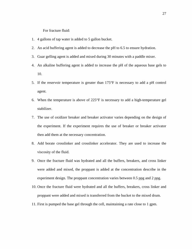
For fracture fluid:
1. 4 gallons of tap water is added to 5 gallon bucket.
2. An acid buffering agent is added to decrease the pH to 6.5 to ensure hydration.
3. Guar gelling agent is added and mixed during 30 minutes with a paddle mixer.
4. An alkaline buffering agent is added to increase the pH of the aqueous base gels to
10.
5. If the reservoir temperature is greater than 175°F is necessary to add a pH control
agent.
6. When the temperature is above of 225°F is necessary to add a high-temperature gel
stabilizer.
7. The use of oxidizer breaker and breaker activator varies depending on the design of
the experiment. If the experiment requires the use of breaker or breaker activator
then add them at the necessary concentration.
8. Add borate crosslinker and crosslinker accelerator. They are used to increase the
viscosity of the fluid.
9. Once the fracture fluid was hydrated and all the buffers, breakers, and cross linker
were added and mixed, the proppant is added at the concentration describe in the
experiment design. The proppant concentration varies between 0.5 ppg and 2 ppg.
10. Once the fracture fluid were hydrated and all the buffers, breakers, cross linker and
proppant were added and mixed is transferred from the bucket to the mixed drum.
11. First is pumped the base gel through the cell, maintaining a rate close to 1 gpm.

28
12. Switch the proper valves to change from the base gel to fracture fluid. Maintain an
optimum rate to avoid plug the pipe and to protect the centrifugal pump.
13. Close the valves at the inlet and outlet of the cell when proppant distribution is lower
than the original at the beginning of the injection. Use the bypass to clean the line
and pump water for 20 minutes to protect the pump.
14. During pumping, the pipe and the cell were heated using a heating tape and heating
jacket at predetermined temperature, a J type thermocouple control the fluid
temperature inside the pipe. The fluid is collected in a waste drum.
15. The schematic of the apparatus for conductivity measurements is shown Figure 11.
Heating tape
Figure 11—Schematic representation of fracture conductivity experiment.

29
2.4.4 Closure Stress Shut-in
Closure stress is the pressure at which the fracture closes after the fracturing
pressure is relaxed, is determined by the overburden pressure (a function of depth and
rock density), pore pressure, Poisson's Ratio, porosity, tectonic stresses, and anisotropy.
Rocks with high closure stress are harder to frac (take more horsepower) than the same
rocks with lower closure stress.
During this experiment the closure stress shut in procedure is as follows:
1. Open the windows interface GCTS C.A.T.S. Standard.
2. In the upper pane, click on File, Projects.
3. The Project/Sample/Specimen window will be open.
4. Click on RPSEA project or create a new project.
5. Click on RPSEA-TEST sample or create a new sample.
6. Click on New specimen and type the information required and then click OK.
7. The Universal Test Setup window will be open. Click on one of the programs or
click on New to create a new program.
8. The information necessary is Duration (time of the test), Data Acquisition (record
data at time interval), and finally Ramp, to chose the ramp type time and pressure.
Click OK.
9. On the Universal Test-Control window click Run to start the closure stress
simulation.
During the length of time of the test, the hydraulic frame will apply a force over
the large surface area of the cell, simulating in this way the formation closure stress.

30
2.4.5 Fracture Conductivity Procedure
1. Measuring fracture conductivity is a long process that can take up to 48 hours. Below
is the procedure for measuring fracture conductivity.
2. Follow the guideline for core preparation, rock permeability measurement, and fluid
pumping. Before start the procedure for measuring fracture conductivity is necessary
to calibrate the pressure transducer.
3. To calibrate the pressure transducers open the windows interface GCTS C.A.T.S.
Standard.
4. In the upper pane, click on System, Inputs, Analog the Analog Inputs window will be
open.
5. To calibrate the pressure inside the cell click on Al-4: Abs Pressure on the Analog
the Analog Inputs window.
6. Click on Calibrate, the window Calibration Type Selection will be open.
7. Select 2 point, next select the max and min pressure of the diaphragm to use in the
pressure port and then click Ok. The diaphragm to use to measure absolute pressure
needs to read pressures between 0 and 100 psi.
8. Connect the pressure transducer to a nitrogen source with a reference gauge, set the
First Calibration Point in zero psi and click Next when the reference gauge will be
zero. Set the Second Calibration Point in 50 psi and click Next when the reference
gauge will be 50 psi. Repeat the first and second calibration points and then click Ok.
9. To calibrate the differential pressure inside the cell click on Al-5:_Diff Pressure on
the Analog Inputs window.

31
10. Click on Calibrate, the window Calibration Type Selection will be open.
11. Select 2 point, select the max and min pressure of the diaphragm to use and click Ok.
12. Connect the pressure transducer to a nitrogen source with a reference gauge, set the
First Calibration Point in zero psi and click Next when the reference gauge will be
zero. Set the Second Calibration Point in 40% of the maximum pressure of the
diaphragm to calibrate and click Next when the reference gauge get the pressure.
Repeat the first and second calibration points and then click Ok.
13. Connect the pressure transducers to the ports of the cell. Once the pressure
transducers are calibrated and the closure stress is applied to the cell, the procedure
continues to measure fracture conductivity.
14. Open the valves next to the pressure ports and at the inlet and outlet of the cell, let
for 5 minutes to relax the pressure and record values for absolute pressure and
differential pressure.
15. Open the nitrogen regulator and mass flow controller to flow gas into the
conductivity cell.
16. Check all lines for leakage. Close the nitrogen regulator if leakage is found and
repair the leak.
17. Adjust nitrogen regulator, back pressure regulator, and mass flow controller until the
cell pressure reading reaches 50 psi and the gas flow rate reaches 2 slm.
18. Wait until flow rates and pressure readings stabilize and record the gas flow rate, cell
pressure, and differential pressure.

32
19. Vary the gas flow rate from 2 to 10 slm to get five data sets at cell pressure of 50 psi.
To increase gas flow rate, open the nitrogen regulator.
20. After reading 5 points, close the nitrogen regulator up to get a continue flow of
nitrogen at a low predetermined rate for a predetermined time.
21. After flowing nitrogen at the predetermined rate for certain time (in this experiments
2 hours), repeat step 15 to 18 to get data points for the fracture conductivity
calculation.
22. Once the test is finish, turn off the nitrogen flow and disconnect all lines to the
conductivity cell.
23. Remove the rock sample from the cell with the hydraulic jack.
24. Calculate the fracture conductivity by using Forcheimer’s equation.
25. To calculate fracture conductivity (kfw) from the experimental data, the
Forcheimer’s equation Eq. 2.1 can be arranged as a straight line
equation , using
as the x-axis and as the y-axis. The y-intercept is the inverse of the
fracture conductivity (kfw). Pressure drop and cell pressure was measured
along the fracture under five different gas flow rates. Fracture conductivity was
measured at different times to study the fracture fluid clean up characteristic and gel
damage.
The schematic of the apparatus for conductivity measure test is shown Figure 12.

33
The variables used in Forcheimer’s equation for conductivity calculations are:
(h) Width of fracture face 1.75 in
(L) Length over pressure drop 5.25 in
(z) Compressibility factor 1.00
(R) Universal constant 8.3144 J/molK
(T) Temperature 293.15 K
(M) RMM of nitrogen 0.028 kg/kg mole
(µ) Viscosity of nitrogen 1.759E-05 Pa s
( Density of nitrogen 1.16085 kg/
Figure 12—Schematic representation of conductivity measure test.

34
2.5 Experimental Conditions
In order to simulate thigh gas field conditions as accurately as possible and
obtain valuable test results that could help the design of future hydraulic treatments,
different test parameters were taken into account. These parameters and test conditions
will be explained below.
2.5.1 Rock Sample
The rock used for the experiments was Ohio sandstone. This rock is quarried
sandstone of low permeability with minimal clay reaction. The permeability of the Ohio
sandstone core samples tested was between 0.012 and 0.015 mD.
2.5.2 Fracturing Fluid Composition
The fracturing fluids were mixed following the recipe with the desired polymer
and other additives concentrations. The fluid composition was selected and provided by
a service company for this experiment. This fracturing fluid was selected due to its
similarity to the actual fracturing job operations in tight gas sands. All experiments were
conducted at room temperature during the fluid preparation and injected into the
conductivity cell at the desired temperature. The composition of the fracturing fluids
used for the series of experiment is shown in Table 3.
The components for the selected fracturing fluid are as follows:
• Guar: Is a polymer used to formulate linear gels. This polymer is a dry powder that
hydrates or swells when mixed with an aqueous solution and form a viscous gel.
• pH buffer: The buffer consistently maintains optimal fluid pH required for hydration
and crosslink.

35
• Gel stabilizer: Increases the temperature stability of gelled fracturing fluids, resulting
in a long-lasting, high-viscosity fluid at temperature.
• Breaker: Is a strong oxidizer who decreases the viscosity of fracture fluids.
• Crosslinker: Increase the fluid viscosity using borate ions to crosslink the hydrated
polymers.
• Crosslink accelerator: Increase the crosslink velocity.
2.5.3 Proppant Size and Concentration
Proppant used in this experiment is lightweight ceramic proppant with a mesh
size of 30/50. Since we will not study the effect of proppant size, 30-50 mesh proppant is
appropriate to achieve the objective of this research. The concentration of proppant vary
from 0.5 to 2 ppg, this range was decided because most of the “slickwater” or
“waterfrack” treatments typically uses this low proppant concentrations.
2.5.4 Temperature
To replicate tight gas reservoir conditions, a range of temperature between 150°F
and 250°F have been selected. The reservoir temperature has a large effect on fracture
fluid properties and on proppant properties which leads to effects on fracture
conductivity.
2.5.5 Nitrogen Gas Flow Rate
To simulate gas production from the fracture into the wellbore, wet nitrogen was
used in these experiments. A flow rate for the laboratory setup was calculated to
simulate a field production rate.

36
Table 4 is a comparison between field and laboratory conditions
Table 4—Comparison between field and laboratory conditions.
Laboratory Field
Fracture height (in) 1.6 100
Fracture width (w) 0.04 0.25
Temperature (°F) 150-250 250
Pressure (psi) 50 1000
Using the rate of gas at standard conditions, the rate at field conditions can be
obtained.
Next are the steps and equations necessary to obtain the rate from laboratory to
field.
1.
2.
3.
4.
5.

37
6.
7.
Table 5—Scale flow rates for different reservoir flow rates at different temperatures.
q (slm) q (scf/min) Bg @ 150 q (cf/min) v lab Bg q (cf/min) q (SCF/day)
0.5 0.02 0.34 0.01 13.70 0.02 28.53 2.05E+06
3 0.11 0.34 0.04 82.18 0.02 171.20 1.23E+07
q (slm) q (scf/min) Bg @ 300 q (cf/min) v lab Bg q (cf/min) q (SCF/day)
0.5 0.02 0.43 0.01 17.06 0.02 35.55 2.55E+06
3 0.11 0.43 0.05 102.38 0.02 213.30 1.53E+07
Table 5 shows the results of the scaled flow rates for different reservoir flow
rates at different temperatures.
2.5.6 Closure Stress Loading – Shut-in Time
The stress conditions implemented during the experiment to simulate the
formation closure stress were 3000 psi and 6000 psi. These values were established as a
low and a maximum value from conditions in tight gas reservoirs. The shut in time was
10 hours, this time was selected due to the fact that polymer is designed to break in
approximately 5 hours.

38
CHAPTER III
EXPERIMENTAL RESULTS AND DISCUSSION
A series of fracture conductivity experiments were run in which different
parameters were tested. These experiments were run using the procedure detailed in
Chapter II. The parameters tested were temperature, closure stress, nitrogen flow rate,
polymer loading, breaker concentration and proppant concentration. In order to
minimize the number of experimental runs, maximize the information of every
experiment and identify those factors with large effects on fracture conductivity, a
statistical analysis knows as fractional factorial design methodology was implemented.
With the objective of finding the influences of these parameters, the design
includes sixteen different fracture conductivity experiments under different conditions.
Additionally, a detailed analysis is conducted over these three parameters, polymer
loading, breaker concentration and nitrogen rate. The other parameters, closure stress,
temperature and proppant concentration, are analyzed and explained in the thesis
developed by Pieve 2011.
The conductivity value of several experiments, experimental data and
photographs are presented in Appendix A.
3.1 Experimental Design
The results of this statistical analysis will help to determine the influence of the
parameters on fracture conductivity. In order to minimize the number of experimental

39
runs it is necessary design a series of experiments using two values for every parameter,
one low factor and one high factor. The factors are listed in Table 6.
Table 6—Low and high factor indicator.
The design displayed in the Table 7 below show the conditions used in each
experiment and the fracture conductivity value measured.
Table 7—Experiment schedule. Exp. N2
Rate (SL/mi
n)
Temperature (°F)
Polymer loading (lb/1000
gal)
Breaker concentrati
on
Closure stress (psi)
Proppant conc. (ppa)
Fracture conductivity (md-ft)
1 0.5 150 10 No 6000 2 531.95 2 0.5 150 30 Normal 2000 0.5 1226.69 3 0.5 250 10 Normal 2000 2 2011.77 4 0.5 250 30 No 6000 0.5 15.20 5 3 150 10 Normal 6000 0.5 960.00 6 3 150 30 No 2000 2 1060.87 7 3 250 10 No 2000 0.5 1098.58 8 3 250 30 Normal 6000 2 155.87 9 3 250 30 Normal 2000 0.5 688.75 10 3 250 10 No 6000 2 118.23 11 3 150 30 No 6000 0.5 15.30 12 3 150 10 Normal 2000 2 1477.00 13 0.5 250 30 No 2000 2 959.10 14 0.5 250 10 Normal 6000 0.5 476.03 15 0.5 150 30 Normal 6000 2 1232.19 16 0.5 150 10 No 2000 0.5 2485.40
N2 Rate (SL/min)
Temperature (°F)
Polymer loading
(lb/1000 gal)
Breaker concentration
Closure stress (psi)
Proppant conc. (ppa)
High 3.0 250 30 Normal 6000 2.0 Low 0.5 150 10 No 2000 0.5

40
3.2 Polymer Loading Effect
The fracturing fluid and reservoir characteristics used in this investigation are
similar to the fluid used in the field in tight gas reservoirs. The fluid used in fracture
treatments in this type of reservoirs is denominated by slick water. This fluid uses a low
concentration of polymer. This investigation use two different polymer loadings, 10
lb/1000gal as a low value and 30lb/1000gal as high value.
The experiments were run modifying several parameters in order to observe the
effect of every parameter in fracture conductivity. Figure 13 illustrates how, comparing
the experiments ran with two different polymer loadings (10 lb/1000gal and 30
lb/1000gal) and under similar conditions of closure stress and temperature, polymer
concentration has a direct effect on fracture conductivity.
The first set of experiments (1, 4, 8, 10, 11 and 14) showed a large difference in
conductivity when polymer concentration is changed. These tests were run at high
closure stress and temperature conditions. It was evidenced that experiment at a polymer
loading of 30 lb/1000gal and a combination of high closure stress (6000 psi) and high
temperature (250°F) has a polymeric cake inside the fracture. More residual gel is
deposit inside the fracture at increased the polymer loading, creating this polymeric
damage, reducing significantly fracture conductivity.

41
Figure 13—Comparison between experiments at 30 lb/1000gal and 10 lb/1000gal of polymer loading.
The gel damage may be characterized as the blocking of pore throats by
unbroken viscous gel having limited mobility or, by insoluble polymer fragments. The
proppant and residual gel are compacted by effect of high closure stress and high
temperature, forming the cake outlined (Figure 14). The conductivity value for this
experiment is extremely low (Figure 15), in reality, this conditions unsuccessful fracture
job with extremely under performed gas rates.

42
Figure 14—Cake formed by proppant and residue gel.

43
0
2
4
6
8
10
12
14
16
18
0 5 10 15 20 25 30
Kf-
w (m
d-f
t)
Time (hours)
Fracture conductivity
Figure 15—Fracture conductivity measurement.
When the fracture fluid with a polymer loading of 10 lb/1000gal was under high
closure stress and high temperature (6000 psi and 250°F) the cake was not formed or
formed in too small amounts. This can be explained because when a lower polymer
loading was used, a small amount of residue gel was settled inside the fracture. Figure 16
shows a clean proppant pack and not extended cake observed.
The results confirm the positive effect on final fracture conductivity when a low
polymer loading is used in a fracturing fluid. The main properties of the fracturing fluid
observed in these experiments are the efficiency of the fluid to break and the
effectiveness of the fluid to transport proppant. The experiments show that the use of
less polymer concentration in the fluid does not affect the fluid property of proppant
transportation and the amount of proppant inside the fracture when the fluid with 10

44
lb/1000gal was used is similar at the amount placed by the higher polymer loading fluid
(30 lb/1000gal) (Figure 17).
Figure 16—Proppant pack without polymer cake.

45
Instead, the amount of residue gel when the polymer loading increase in the
fracturing fluid has a direct damage effect to the conductivity inside the fracture, as
observed in Figure 14 and Figure 16.
30 lb/1000gal and 2 ppg
10 lb/1000gal and 2 ppg
Figure 17—Proppant pack comparison using fluids with two different polymer loading.

46
3.3 Breaker Concentration Effect
The breaker is added to the fracturing fluid to reduce the viscosity of the
polymer-based carrier fluid, reducing the molecular weight of the polymer by cutting the
long polymer chains, in order to remove it from the fracture after the stimulation
treatment is completed. When the residual gel can not be removed, it causes damage to
the proppant pack conductivity. Several experiments were carried out using fracturing
fluids with normal concentration of breaker or no breaker at all to examine the effect of
breaker on resulting conductivity.
The comparison between experiments designed with different breaker
concentration is shown in Figure 18. At high conditions of closure stress and
temperature, the final value of fracture conductivity is higher when breaker is added to
the fracturing fluid than when is not used. When experiments with and without breaker
are ran at lower values of closure stress (2000 psi) and similar conditions of polymer
loading and proppant concentration, the final fracture conductivity has similar value.
Previous researches and analysis show that the presence of breaker has a positive
effect on final fracture conductivity. It means when breaker is added to the fracturing
fluid, the final fracture conductivity is higher than when no breaker is added to the fluid.
The results from the experiments in this research show that at simulated higher reservoir
conditions the effect of breaker on fracture conductivity is highly positive and when the
closure stress is low the effect is not so evident.

47
Normal breaker concentration
No breaker concentration
Figure 18— Comparison experiments with and without breaker.
3.4 Gas Flow Rate Effect
The general trend is higher gas flow rate increase the gel cleanup and fracture
conductivity. Figure 19 represents fracture conductivity behavior for different
experimental at similar reservoir and fluid conditions at different gas flow rates. The
experimental data showed that the influence on gel cleanup efficiency is similar at
different gas flow rates and high energy from gas flux is necessary to clean up the
fracture. It was observed that flow rate does not have a significant effect on fracture
clean up, which is opposite to what Marpaung (2007) conclude from his study.
The main reason of disagreement is probably due to the design of the
experiments. The principal objective of the design of the experiments was to identify the
effect of several parameters in fracture conductivity, and probably the effect of gas flow

48
rate was limited on the final design of the experiments. The next step of experiments will
aim to find the role of gas rate and the interaction between gas rate and low polymer
loadings. Once these experiments are successfully completed, the information from this
research could be more study in detailed and accuracy conclusions will be formulated.
Exp 11
Exp 10Exp 8
Exp 9Exp 5
Exp 12
Exp 6Exp 7
Exp 4
Exp 14Exp 1
Exp 13Exp 2 Exp 15
Exp 3
Exp 16
10
100
1000
10000
3 slm
0.5 slm
Fra
ctur
e co
nduc
tivity
(m
d-ft)
Figure 19— Comparison experiments at different gas flow rates.

49
CHAPTER IV
CONCLUSIONS AND RECOMMENDATIONS
4.1 Conclusions
Fracture conductivity tests were conducted under different conditions of
temperature, proppant and polymer loading, gas rate, breaker concentration and closure
stress. The following conclusions are made based on the statistical analysis and the
results from experiments:
1. A dynamic conductivity testing apparatus was modify from the experimental
apparatus used by Marpaung and Pongthunya (Marpaung, 2007; Marpaung et al.,
2008; Pongthunya, 2008) to study the effects of high temperature (up to 250°F) and
high closure stress (up to 6000 psi) on proppant pack conductivity and low polymer
fluid. The new methodology permits the use of low polymer loading fluids and low
proppant loading. Additionally new equipment was added allowing an accuracy
application of closure stress during a specific time and better accuracy of pressure
when fracture conductivity is measure.
2. The number of experiments and conditions of the experiments were design using an
experimental strategy based on fractional factorial design methodology. The
statistical analysis completed in this research is the first step that will lead to
determine with more accuracy the effect of fracture fluid and its additives and the
reservoir conditions on fracture conductivity.

50
3. An analysis and conclusions about the effect of pressure, temperature and proppant
concentration on fracture conductivity can be obtained in the document named
“Laboratory study to identify the impact of fracture design parameters over the final
fracture conductivity using the dynamic fracture conductivity test procedure”. In this
chapter is presented the analysis of polymer loading concentration, breaker
concentration and gas flow rate using the information obtained from the
experimental tests.
4. Polymer concentration has a clear, but small impact on fracture conductivity. Higher
polymer concentration will decrease cleanup efficiency. When polymer loading is
increased in fracture fluid, the gel residue concentration in the fracture after closure
increased too. The gel residue blocks the pore throats by unbroken viscous gel and
by insoluble polymer fragments. At high closure stress and temperature, higher
polymer concentration results in more obvious damage on proppant pack.
5. The use of breaker in fracture fluid increases cleanup efficiency, although, does not
have a great impact on fracture conductivity when the simulated reservoir conditions
are not extreme. The data from the experiments shows that when breaker was added
to fracture fluid the clean up was better.
6. The analysis of nitrogen flow rate on cleanup efficiency and final value of fracture
conductivity does not provide clear conclusion to support the previously published
results. The previous conclusion was higher gas flux increases gel cleanup
efficiency, although, in this research apparently the drag force at different flow rates
was similar and the clean up was comparable.

51
7. As was outlined on 3.6, more experiments specifically design to describe the effect
of gas rate, will be needed support this observations, as well the necessity of increase
the accuracy on the gas rate control adding new equipment and reviewing the
procedure in order to get more reliability.
4.2 Recommendations
The performing of dynamic conductivity testing experiments in a laboratory
facility was successful, and the information collected in this tests can gives more
representative field conditions than previous experiment. The experiments conducted
produced many conclusions; however, additional testing under different conditions
would add further valuable conclusions.
However, there is also some equipment that could be added to make the
procedure of the experiment more consistent. A pump with capacity to pump slurry at
high pressure and high volume is needed. An electronic feedback controller to regulate
the gas flow rate also will reduce the potential for inconsistencies. The combination of
these devices, along with a proper set up would automate a large portion of the
experiment and will lead to a better understand of the parameters effect.
In order to study the influence of different variables on fracture conductivity in
this investigation, an experimental design was used, but for further experiments some
parameters would be considered constants in order to compare the results when just one
parameter is varied.
As an additional part, the comparison of experimental fracture conductivity with
the information of treatments from the field will help to set a more accurately

52
experiment design and will reflect a better understanding of fracturing fluid clean up
characteristic.
A phase behavior analysis could be developed to investigate the effect of
fracturing fluid and residual gel at reservoir conditions.

53
REFERENCES
Almond, S.W. and Bland, W.E. 1984. The Effect of Break Mechanism on
Gelling Agent Residue and Flow Impairment in 20/40 Mesh Sand. Paper SPE 12485
presented at the SPE Formation Damage Control Symposium, Bakersfield, California,
USA, 13-14 February. doi:10.2118/12485-MS.
API RP 60, 1995. Recommended Practices for Testing High-Strength Proppants
Used in Hydraulic Fracturing Operations, second edition. Washington, DC: API.
API RP 61, 1989. Recommended Practice for Evaluating Short-Term Proppant-
Pack Conductivity, first edition. Washington, DC: API.
Cooke Jr., C.E. 1975. Effect of Fracturing Fluids on Fracture Conductivity. J.
Pet. Technol. 27 (10): 1273-1282. SPE-5114-PA.doi: 10.2118/5114-PA.
Freeman, E.R., Anschutz, D.A., Rickards, A.R. et al. 2009. Modified Api/Iso
Crush Tests with a Liquid-Saturated Proppant under Pressure Incorporating
Temperature, Time, and Cyclic Loading: What Does It Tell Us? Paper SPE 118929
presented at the SPE Hydraulic Fracturing Technology Conference, The Woodlands,
Texas, 19-21 January. doi: 10.2118/118929-MS.
Hawkins, G.W. 1988. Laboratory Study of Proppant-Pack Permeability
Reduction Caused by Fracturing Fluids Concentrated During Closure. Paper SPE 18261
presented at the 1988 SPE Annual Technical Conference and Exhibition, Houston,
Texas, 2-5 October. doi: 10.2118/18261-MS.

54
Kaufman, P.B., Anderson, R.W., Parker, M.A. et al. 2007. Introducing New
Api/Iso Procedures for Proppant Testing. Paper SPE 110697 presented at the 2007 SPE
Annual Technical Conference and Exhibition, Anaheim, California, 11-14 November.
doi: 10.2118/110697-MS.
Kim, C.M. and Losacano, J.A. 1985. Fracture Conductivity Damage Due to
Crosslinked Gel Residue and Closure Stress on Propped 20/40 Mesh Sand. Paper SPE
14436 presented at the 1985 SPE Annual Technical Conference and Exhibition, Las
Vegas, Nevada, 22-26 September. doi: 10.2118/14436-MS.
Marpaung, F. 2007. Investigation of the Effect of Gel Residue on Hydraulic
Fracture Conductivity Using Dynamic Fracture Conductivity Test. M.S thesis, Texas
A&M University, College Station, Texas.
Marpaung, F., Chen, F., Pongthunya, P. et al. 2008. Measurement of Gel Cleanup
in a Propped Fracture with Dynamic Fracture Conductivity Experiments. Paper SPE
115653 presented at the 2008 SPE Annual Technical Conference and Exhibition,
Denver, Colorado, 21-24 September. doi: 10.2118/115653-MS.
Much, M.G. and Penny, G.S. 1987. Long-Term Performance of Proppants under
Simulated Reservoir Conditions. Paper SPE 16415 presented at the Low Permeability
Reservoirs Symposium, Denver, Colorado, 18-19 May. doi: 10.2118/16415-MS.
Parker, M.A. and McDaniel, B.W. 1987. Fracturing Treatment Design Improved
by Conductivity Measurements under in-Situ Conditions. Paper SPE 16901 presented at
the 1987 SPE Annual Technical Conference and Exhibition, Dallas, Texas, 27-30
September. doi: 10.2118/16901-MS.

55
Pongthunya, P. 2007. Development, Setup and Testing of a Dynamic Hydraulic
Fracture Conductivity Apparatus.M.S thesis, Texas A&M University, College Station,
Texas.
Roodhart, L.P. 1985. Fracturing Fluids: Fluid-Loss Measurements under
Dynamic Conditions. SPE J. 25 (5): 629-636. SPE-11900-PA. doi: 10.2118/11900-PA.
U.S. Department of Energy. 2008, Unconventional Gas Production in the United
States., E.i.A. http://www.eia.doe.gov/. Accessed 12 October 2008.
van der Vlis, A.C., Haafkens, R., Schipper, B.A. et al. 1975. Criteria for Proppant
Placement and Fracture Conductivity. Paper SPE 5637 presented at the Fall Meeting of
the Society of Petroleum Engineers of AIME, Dallas, Texas, 28 September-1 October.
doi: 10.2118/5637-MS.
Volk, L.J., Gall, B.L., Raible, C.J. et al. 1983. A Method for Evaluation of
Formation Damage Due to Fracturing Fluids. Paper SPE 11638 presented at the
SPE/DOE Low Permeability Gas Reservoirs Symposium, Denver, Colorado, 14-16
March. doi: 10.2118/11638-MS.

56
APPENDIX A
A.1 Experiment Schedule
Table 8–Experiment schedule and results. Exp. N2 Rate
(SL/min) Temperature
(°F) Polymer loading
(lb/1000 gal)
Breaker concentration
Closure stress (psi)
Proppant conc. (ppa)
Fracture conductivity
(md-ft) 1 0.5 150 10 No 6000 2 531.95 2 0.5 150 30 Normal 2000 0.5 1226.69 3 0.5 250 10 Normal 2000 2 2011.77 4 0.5 250 30 No 6000 0.5 15.20 5 3 150 10 Normal 6000 0.5 960.00 6 3 150 30 No 2000 2 1060.87 7 3 250 10 No 2000 0.5 1098.58 8 3 250 30 Normal 6000 2 155.87 9 3 250 30 Normal 2000 0.5 688.75 10 3 250 10 No 6000 2 118.23 11 3 150 30 No 6000 0.5 15.30 12 3 150 10 Normal 2000 2 1477.00 13 0.5 250 30 No 2000 2 959.10 14 0.5 250 10 Normal 6000 0.5 476.03 15 0.5 150 30 Normal 6000 2 1232.19 16 0.5 150 10 No 2000 0.5 2485.40

57
A.1.1 Experiment 1
0
100
200
300
400
500
600
0 5 10 15 20 25 30 35
Kf-
w (m
d-ft)
Time (hours)
Figure 20–Fracture conductivity vs time. Experiment 1.
Figure 21–Proppant placed. Experiment 1.

58
A.1.2 Experiment 12
0
200
400
600
800
1,000
1,200
1,400
1,600
1,800
0 5 10 15 20 25 30
Kf-
w (m
d-f
t)
Time (hours)
Figure 22–Fracture conductivity vs time. Experiment 12.
Figure 23–Proppant placed. Experiment 12.

59
A.1.3 Experiment 9
0
100
200
300
400
500
600
700
800
0 5 10 15 20 25 30
Kf-
w (m
d-f
t)
Time (hours)
Figure 24–Fracture conductivity vs time. Experiment 9.
Figure 25–Proppant placed. Experiment 9.

60
A.1.4 Experiment 3
0
500
1,000
1,500
2,000
2,500
3,000
0 5 10 15 20 25 30
Kf-
w (m
d-f
t)
Time (hours)
Figure 26–Fracture conductivity vs time. Experiment 3.
Figure 27–Proppant placed. Experiment 3.

61
VITA
Name: Juan Carlos Correa Castro
Address: Texas A&M University Petroleum Engineering Dept. 3116 TAMU, 501 Richardson Bldg. College Station, TX 77843-3116 Email Address: [email protected] Education: B.S., Petroleum Engineering, Universidad Industrial de Santander, 2000 M.S., Petroleum Engineering, Texas A&M University, 2011 This thesis was typed by the author