Evaluation and Conﬁguration of a Control Loop Asset...

Institutionen för systemteknikDepartment of Electrical Engineering

Examensarbete

Evaluation and Configuration of a Control LoopAsset Monitoring Tool

Examensarbete utfört i Reglerteknikvid Tekniska högskolan vid Linköpings universitet

av

Calle Skillsater

LiTH-ISY-EX--11/4461--SE

Linköping 2011

Department of Electrical Engineering Linköpings tekniska högskolaLinköpings universitet Linköpings universitetSE-581 83 Linköping, Sweden 581 83 Linköping

Evaluation and Configuration of a Control LoopAsset Monitoring Tool

Examensarbete utfört i Reglerteknikvid Tekniska högskolan i Linköping

av

Calle Skillsater

LiTH-ISY-EX--11/4461--SE

Handledare: Andre Carvalho Bittercourtisy, Linkopings universitet

Alf IsakssonABB AB

Examinator: Martin Enqvistisy, Linkopings universitet

Linköping, 29 April, 2011

Avdelning, InstitutionDivision, Department

Division of Automatic ControlDepartment of Electrical EngineeringLinköpings universitetSE-581 83 Linköping, Sweden

DatumDate

2011-04-29

SprakLanguage

� Svenska/Swedish� Engelska/English

�

�

RapporttypReport category

� Licentiatavhandling� Examensarbete� C-uppsats� D-uppsats� Ovrig rapport�

�

URL for elektronisk versionhttp://www.control.isy.liu.sehttp://www.ep.liu.se

ISBN—

ISRNLiTH-ISY-EX--11/4461--SE

Serietitel och serienummerTitle of series, numbering

ISSN—

TitelTitle

Svensk titelEvaluation and Configuration of a Control Loop Asset Monitoring Tool

ForfattareAuthor

Calle Skillsater

SammanfattningAbstract

In this thesis, an automatic control performance monitoring tool is analyzed andevaluated. The tool is called Control Loop Asset Monitor (CLAM) and is a partof the Asset Optimization extension to the ABB platform System 800xA. CLAMcalculates and combines a number of performance indices into diagnoses. Thefunctionality, choice of configuration parameters and the quality of the result fromCLAM have been analyzed using data from the pulp mill Sodra Cell Morrum.

In order to get reliable diagnoses from CLAM, it is important that it is correctlyconfigured. It was found that some of the default parameters should be modifiedand the recommendations in the user guidelines should be updated. Using thecurrent default parameters, there are some combinations of indices that never canexceed defined alarm severity thresholds.

The conclusions in this thesis have been documented in an online help thatalso includes simple user instructions for how the results from CLAM should beinterpreted. The results have been analyzed together with the staff at Sodra CellMorrum in order to validate that they are correct and relevant from a user per-spective. It was found that the results are correct, but there are some things thatcan be improved in order to make CLAM more user friendly.

NyckelordKeywords Control Loop Asset Monitoring, performance, pulp, 800xA, Asset Optimization

AbstractIn this thesis, an automatic control performance monitoring tool is analyzed andevaluated. The tool is called Control Loop Asset Monitor (CLAM) and is a partof the Asset Optimization extension to the ABB platform System 800xA. CLAMcalculates and combines a number of performance indices into diagnoses. Thefunctionality, choice of configuration parameters and the quality of the result fromCLAM have been analyzed using data from the pulp mill Sodra Cell Morrum.

In order to get reliable diagnoses from CLAM, it is important that it is correctlyconfigured. It was found that some of the default parameters should be modifiedand the recommendations in the user guidelines should be updated. Using thecurrent default parameters, there are some combinations of indices that never canexceed defined alarm severity thresholds.

The conclusions in this thesis have been documented in an online help that alsoincludes simple user instructions for how the results from CLAM should be in-terpreted. The results have been analyzed together with the staff at Sodra CellMorrum in order to validate that they are correct and relevant from a user per-spective. It was found that the results are correct, but there are some things thatcan be improved in order to make CLAM more user friendly.

v

Acknowledgments

This thesis has been performed at ABB Corporate Research and Sodra Cell Morrum.It feels like a privilege to have the opportunity to both see the inside of the de-veloper of this tool and a user. Using this approach is really something that I canrecommend.

My work here has been very educating and fun. The main reason for this ismy supervisor Alf Isaksson. Thank you for your patience, enthusiasm and thefreedom you gave me. I also want to thank Christian Johansson for your supportand interest in my work.

Thank you, Martin Enqvist and Andre Carvalho Bittercourt at Linkoping Univer-sity for your support and all help with my report.

I would also like to thank Sodra Cell Morrum for giving me the opportunity to seehow things work in reality. Thank you, Gert Svensson and Magnus Andersson foryour patience and support.

Finally, I want to thank my family and friends. Thank you, Elise, Maths, Anne,Jonna and Sunny. Without you, I would not have been where I am today.

Calle SkillsaterVasteras, April 2011

vii

Contents

1 Introduction 11.1 Background . . . . . . . . . . . . . . . . . . . . . . . . . . . . . . . 11.2 Goal . . . . . . . . . . . . . . . . . . . . . . . . . . . . . . . . . . . 31.3 Limitations . . . . . . . . . . . . . . . . . . . . . . . . . . . . . . . 31.4 Thesis Outline . . . . . . . . . . . . . . . . . . . . . . . . . . . . . 3

2 Pulp Production Process at Sodra Cell Morrum 52.1 Process Overview . . . . . . . . . . . . . . . . . . . . . . . . . . . . 52.2 Wood . . . . . . . . . . . . . . . . . . . . . . . . . . . . . . . . . . 62.3 Barking and Chipping . . . . . . . . . . . . . . . . . . . . . . . . . 72.4 Digesting . . . . . . . . . . . . . . . . . . . . . . . . . . . . . . . . 72.5 Washing and Filtrering . . . . . . . . . . . . . . . . . . . . . . . . . 72.6 Bleaching . . . . . . . . . . . . . . . . . . . . . . . . . . . . . . . . 82.7 Drying . . . . . . . . . . . . . . . . . . . . . . . . . . . . . . . . . . 82.8 Chemical Recovery . . . . . . . . . . . . . . . . . . . . . . . . . . . 8

3 Control System at Sodra Cell Morrum 93.1 System 800xA Platform . . . . . . . . . . . . . . . . . . . . . . . . 93.2 Control Equipment . . . . . . . . . . . . . . . . . . . . . . . . . . . 103.3 RegDoc . . . . . . . . . . . . . . . . . . . . . . . . . . . . . . . . . 103.4 History Logging . . . . . . . . . . . . . . . . . . . . . . . . . . . . . 11

4 Causes of Malfunctioning Control Loops 134.1 Static Friction (Stiction) . . . . . . . . . . . . . . . . . . . . . . . . 134.2 Dead-band . . . . . . . . . . . . . . . . . . . . . . . . . . . . . . . 144.3 Backlash . . . . . . . . . . . . . . . . . . . . . . . . . . . . . . . . . 144.4 Saturation . . . . . . . . . . . . . . . . . . . . . . . . . . . . . . . . 144.5 Quantization . . . . . . . . . . . . . . . . . . . . . . . . . . . . . . 154.6 External Causes . . . . . . . . . . . . . . . . . . . . . . . . . . . . 164.7 Other Reasons . . . . . . . . . . . . . . . . . . . . . . . . . . . . . 16

5 Control Loop Performance Monitoring 175.1 Tool Requirements . . . . . . . . . . . . . . . . . . . . . . . . . . . 175.2 Performance Indices . . . . . . . . . . . . . . . . . . . . . . . . . . 18

ix

x Contents

5.3 Control Loop Asset Monitoring Tool within System 800xA . . . . . 185.3.1 Configuration . . . . . . . . . . . . . . . . . . . . . . . . . . 23

6 Analyses of Configuration Parameters 256.1 Data Set Size . . . . . . . . . . . . . . . . . . . . . . . . . . . . . . 256.2 Data Interval . . . . . . . . . . . . . . . . . . . . . . . . . . . . . . 276.3 CO low/CO high . . . . . . . . . . . . . . . . . . . . . . . . . . . . 286.4 Cascade . . . . . . . . . . . . . . . . . . . . . . . . . . . . . . . . . 286.5 PV low/PV high . . . . . . . . . . . . . . . . . . . . . . . . . . . . 296.6 Weight Parameters . . . . . . . . . . . . . . . . . . . . . . . . . . . 30

6.6.1 Final Control Element Summary Weights . . . . . . . . . . 306.6.2 Loop Performance Summary Weights . . . . . . . . . . . . 31

6.7 Thresholds . . . . . . . . . . . . . . . . . . . . . . . . . . . . . . . 326.7.1 Severity Thresholds . . . . . . . . . . . . . . . . . . . . . . 326.7.2 Alarm Thresholds . . . . . . . . . . . . . . . . . . . . . . . 33

6.8 Filter Parameters . . . . . . . . . . . . . . . . . . . . . . . . . . . . 336.9 Dead Time . . . . . . . . . . . . . . . . . . . . . . . . . . . . . . . 376.10 Loop Category . . . . . . . . . . . . . . . . . . . . . . . . . . . . . 416.11 Resample Interval . . . . . . . . . . . . . . . . . . . . . . . . . . . 426.12 Aggregate Function . . . . . . . . . . . . . . . . . . . . . . . . . . . 426.13 Inhibit Value . . . . . . . . . . . . . . . . . . . . . . . . . . . . . . 42

7 History Logging 437.1 OPC Direct Logging with 3 Seconds Cyclic Rate . . . . . . . . . . 437.2 Effects on CLAM Results . . . . . . . . . . . . . . . . . . . . . . . 497.3 Size Analyses of History Log . . . . . . . . . . . . . . . . . . . . . 50

8 Validation of Results from CLAM 538.1 PC451029 . . . . . . . . . . . . . . . . . . . . . . . . . . . . . . . . 538.2 LC471640 . . . . . . . . . . . . . . . . . . . . . . . . . . . . . . . . 568.3 LC482122 . . . . . . . . . . . . . . . . . . . . . . . . . . . . . . . . 578.4 FC542024 . . . . . . . . . . . . . . . . . . . . . . . . . . . . . . . . 588.5 FC442064 . . . . . . . . . . . . . . . . . . . . . . . . . . . . . . . . 60

9 Online Help 659.1 Outline of the Online Help . . . . . . . . . . . . . . . . . . . . . . . 65

10 Conclusions 6710.1 Configuration Parameters . . . . . . . . . . . . . . . . . . . . . . . 6710.2 History Logging . . . . . . . . . . . . . . . . . . . . . . . . . . . . . 6810.3 Validation of Results from CLAM . . . . . . . . . . . . . . . . . . 69

11 Future Work 71

A Performance Indices 75

B Indices vs. Parameters 81

Contents xi

C Indices vs. Logging Interval 83

D Dead Time Histograms 87

E Result from Index Layer for FC442064 91

Chapter 1

Introduction

In this chapter, the background of this thesis is described. For more detailedinformation about the production process see Chapter 2 and Chapter 5 for moredetails about control loop performance monitoring.

This thesis has been a combination of two worlds. The major part of the work hasbeen done at ABB Corporate Research (SECRC) in Vasteras and the remainingat Sodra Cell Morrum. ABB is a worldwide engineering company with productsin many different areas. One such area is automation systems, where the plat-form System 800xA is widely used in industries all over the world. One softwareextension for the 800xA base system is Asset Optimization (AO), which enablesreal-time asset monitoring, notification, etc. The software Control Loop AssetMonitor (CLAM) is one tool included in AO. It enables monitoring of control loopperformance based on advanced combinations of a large amount of performanceindices (ABB, 2003a).

Today, the industries get more complex and automated in combination with agrowing interest in energy savings. A modern process industry may have hundredsor even thousands of control loops and no human can keep track of the maintenanceneed for all of them.

1.1 Background

One user of System 800xA with the AO extension is Sodra Cell Morrum. Theirplant in Morrum is one of five pulp mills in a division of the main organizationSodra called Sodra Cell. The other mills are located in Varo and Monsteras inSweden and Tofte and Folla in Norway. Sodra is owned by 52,000 land owners inthe southern parts of Sweden and does also consist of the divisions Sodra Timber,Sodra Interior and Sodra Skog.

1

2 Introduction

Sodra Cell is one of the world’s leading producers of market pulp with a totalproduction capacity of 2.1 million tons per year. Today the market for bioenergygets more and more important. Sodra delivers 3.7 TWh of green energy each yearand is one of the biggest bioenergy companies in Sweden. At Sodra Cell Morrumthis is delivered as both electricity and heat. Today you can say that from everylog of wood half is turned into pulp and half is used to produce energy (Sodra,2008).

The pulp from Sodra Cell is sold to customers producing almost any paper productyou may think of, from paper board and magazines to tea bags and tissues. About90 percent of their products are sold to customers in Europe, and 10 percent toAsia (mainly China and Thailand). The plant in Morrum contains a large numberof control loops; approximately 1200-1400 loops (Sodra Cell Morrum, 2010b).

It would require an enormous amount of personnel to continuously monitor allloops manually. The need for a tool for automatic monitoring of control loops wassomething that Sodra Cell Morrum realized already in the late 1990’s. Since thenthey have tried a various range of software tools. Some of them did not work asexpected and some were hard to use for people with different levels of competence.Since a few years back they have the System 800xA extension CLAM installed incombination with another ABB tool called Sigma Monitor (Sodra Cell Morrum,2010c). The Sigma monitor performs a simple monitoring of the standard deviationof the control error. CLAM provides information about the loop performanceand the control actuator (called final control element (FCE) in CLAM). The loopperformance analysis includes detection of oscillations, high variance, evaluation ofcascade tracking, etc. The FCE analysis includes detection of high static friction,valve leakage, indications of non-optimal actuator size and FCE nonlinearities.

CLAM is intended to be a complement to the Sigma Monitor for loops of extraimportance. For example, it can be loops with a large and direct effect on theproduct quality, production economy or the environment.

Except continuous monitoring of important control loops Sodra Cell Morrum hasanother need. When a process segment is about to be investigated for possibleimprovement Sodra Cell Morrum wants to have the possibility to use CLAM on allloops in that section. This would result in a pre-study over the segment, makingthe work more efficient as CLAM would give indications on where to put the mostresources.

In order to get a reliable diagnosis from CLAM, it is necessary that the softwareis configured correctly. There are a number of parameters that can be modified toget a monitoring system that is suitable for different types of loops and areas ofuse.

Before this thesis was performed, the staff at Sodra Cell Morrum regarded CLAMas complicated and hard to use. There were no simple guidelines on how to monitora new loop and how the result from CLAM should be interpreted.

1.2 Goal 3

1.2 Goal

The goal with this thesis is to clarify how CLAM should be configured for differenttypes of control loops in order to get reliable diagnoses. The result should be for-mulated into guidelines and organized in an online help feature. The reliability ofthe CLAM diagnoses should thereby be increased and the configuration simplifiedfor the customers.

Sodra Cell Morrum should finally be supplied with a reliable tool for control loopperformance monitoring that is easy to configure and interpret for the users. Thevision with this project is to make CLAM a better product with increased valuefor the customers.

1.3 Limitations

There exist some limitations regarding the data logging. At Sodra Cell Morrumthe history log is divided into 3 parts with different logging density and only 3signals per loop are logged:

• The data are logged for 8 hours with a sampling interval of 5 seconds. After8 hours the data are logged for 7 days with an interval of 15 seconds, whereevery stored value is an average of three 5 second samples. Finally, the dataare logged for 30 days with an interval of 1 minute where every stored valueis an average of four 15 second samples.

• The logged information consists only of controller output (CO), process value(PV) and setpoint (SP).

1.4 Thesis Outline

In the next chapter, the process of pulp production at Sodra Cell Morrum is de-scribed in more detail. In Chapter 3, the System 800xA and the control equipmentat Sodra Cell Morrum are described. Possible causes of malfunctioning controlloops and control loop performance monitoring are described in Chapter 4 and5. In Chapter 6, results from analyses of how CLAM should be configured aredescribed. An analysis of history logging is described in Chapter 7 and in Chap-ter 8 results from CLAM are validated. In the final chapters, conclusions andsuggestions for future work are described.

Chapter 2

Pulp Production Process atSodra Cell Morrum

In this chapter, a brief description of the pulp production is given. First, anoverview is presented and all major steps are then described in more detail.

2.1 Process Overview

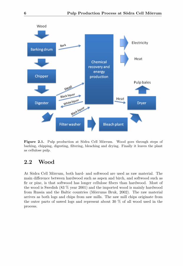
The production process from wood to pulp can be described by Figure 1. Woodgoes through steps of barking, chipping, digesting (cooking), washing and filtering,bleaching and drying. The chemicals used in the process are recycled in a separatepart that also produces electricity and heat. The energy surplus is sold to theregular market and yields money from green certificates on the energy market(Sodra Cell Morrum, 2010a).

The plant at Sodra Cell Morrum consists of two separate production lines due tothe fact that the mill has been upgraded in several phases since the opening in1962. This means that the need of controllers, staff, etc. is increased compared toa plant with the same capacity with one production line.

5

6 Pulp Production Process at Sodra Cell Morrum

Figure 2.1. Pulp production at Sodra Cell Morrum. Wood goes through steps ofbarking, chipping, digesting, filtering, bleaching and drying. Finally it leaves the plantas cellulose pulp.

2.2 Wood

At Sodra Cell Morrum, both hard- and softwood are used as raw material. Themain difference between hardwood such as aspen and birch, and softwood such asfir or pine, is that softwood has longer cellulose fibers than hardwood. Most ofthe wood is Swedish (83 % year 2001) and the imported wood is mainly hardwoodfrom Russia and the Baltic countries (Morrums Bruk, 2002). The raw materialarrives as both logs and chips from saw mills. The saw mill chips originate fromthe outer parts of sawed logs and represent about 30 % of all wood used in theprocess.

2.3 Barking and Chipping 7

2.3 Barking and Chipping

The logs need to be barked before they can be used in the process. Since thebark is not used as raw material in the pulp, it is removed in large barking drums.These drums consist of large rotating cylinders where the logs are rubbed againsteach other and the cylinder walls. The removed bark is a very important sourceof energy that has almost totally eliminated the need of oil for heating at SodraCell Morrum (Morrums Bruk, 2002).

If the barking process does not work properly, the pulp will be impure and morechemicals are needed in the digesting and bleaching steps (Sodra, 2004). Thebarked wood is chipped into small pieces and stored in huge stacks. The cellulosefibers are located inside the wood chips and will later form the pulp, but the fibersare embedded in lignin that has to be removed in the digester.

2.4 Digesting

In the digesting step, the chips are boiled together with cooking chemicals andwater. At Sodra Cell Morrum there are ten such cooking vessels, four for line oneand six for line two (Sodra Cell Morrum, 2010c). The cooking is done batchwise,i.e. the digester is filled with chips and chemicals and left cooking for about fivehours and then the pulp is pumped to a clearance vessel. This procedure differsfrom continuous digesters where chips and chemicals are added and cooked pulpis removed continuously. The cooking chemicals are called white liquor. The mainingredient in white liquor is caustic soda, often used for pipe cleaning in our homes.

During the digesting process bad smelling gases are formed. They are transportedto the soda recovery boiler where they are burned (Sodra, 2004). In this way thenearby environment is less affected and the characteristic “paper mill smell” istoday just a memory from the past. When the cooking is finished the white liquoris polluted by lignin and called black liquor.

2.5 Washing and Filtrering

In the washing and filtering step, the black liquor is separated from the cellulosepulp and proceeds to the recycling step. Except for liquor and lignin, the pulpis mixed with pollutions like residues of bark and twigs. The pulp passes severalsteps of filtering and draining before it is pumped to the bleaching step. Theseparated liquor can be used again after chemical recovery.

8 Pulp Production Process at Sodra Cell Morrum

2.6 Bleaching

The cleaned pulp is very brown in its color. To make the pulp white it has to bebleached. When the mill was new in the 1960s this was done with chlorine gas, buttoday the pulp is bleached with oxygen gas followed by chlorine dioxide (MorrumsBruk, 2002). The bleaching also reduces the percentage of lignin even more.

2.7 Drying

When the pulp reaches the drying step it has a consistency similar to porridge.First the pulp is accumulated and a lot of water percolates away. Then morewater is removed by vacuum suction and by running it through several presscylinders. The pulp is now solid and transported to a drying cabinet, heated bysteam. This step is very energy consuming. After drying, the pulp only consistsof approximately 10 % water and is ready for delivery. This is done when the pulpis cut into sheets and bundled together.

2.8 Chemical Recovery

Black liquor from the digester consists of released wood substances, cooking chemi-cals and about 85 % water. To be able to burn the black liquor in the soda recoveryboiler the water percentage has to be reduced to 25-30 % through several evap-oration steps. In this step sulfate soap is removed. After reaction with acid thesoap turns into pine oil that is used for production of biodiesel.

When the black liquor is burned in the recovery boiler the chemicals react in theheat forming a melt at the bottom. The pollutions burn and generate heat, usablein other parts of the production process. The flue gases are cleaned in severalsteps before they are released through the top of the chimney. The melt at thebottom is pumped to a causticizing step where the white liquor is recovered to beused in the process again.

Chapter 3

Control System at SodraCell Morrum

3.1 System 800xA Platform

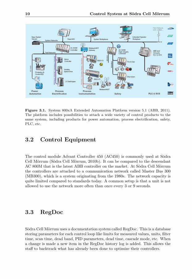
Sodra Cell Morrum uses an ABB automation system called System 800xA. It is aDistributed Control System (DCS) creating a flexible and collaborative platformwith large integration possibilities (ABB, 2008). As can be seen in Figure 2 be-low, control equipment from different suppliers and product generations as well ascontrollers for different purposes can easily be attached to the same network.

The platform can be accessed with different interfaces, customized for operators,engineers, maintenance personnel, etc. This enables the users to concentrate ontheir own task and thereby work more efficiently.

A common issue in the industry today is the cost of modernization. Motivating thecost of upgrading all old equipment is often unthinkable (ABB, 2003b). Thereforethe solution is to build on what you have. As a consequence of this most of thecontrollers at Sodra Cell Morrum are from the product family Advant Master,where they have the latest controller generation called AC450. These controllersare connected to System 800xA through Connectivity Servers, providing data fromthe controllers to operator workplaces, history collection, etc. The installationoutline can be seen in Figure 3. Modern controllers like AC 800M may be installedside by side with older equipment like AC450. This makes it possible for customersto efficiently upgrade their systems and still keep the major parts of their oldersystems.

System 800xA is used in a wide variety of applications that except for Pulp andPaper also include Oil and Gas, Petro Chemical, Biotech/Pharmaceutical, Power,Water, Utilities, Chemicals/Fine Chemicals, Metals, Mining, etc (ABB, 2011).

9

10 Control System at Sodra Cell Morrum

Figure 3.1. System 800xA Extended Automation Platform version 5.1 (ABB, 2011).The platform includes possibilities to attach a wide variety of control products to thesame system, including products for power automation, process electrification, safety,PLC, etc.

3.2 Control Equipment

The control module Advant Controller 450 (AC450) is commonly used at SodraCell Morrum (Sodra Cell Morrum, 2010b). It can be compared to the descendantAC 800M that is the latest ABB controller on the market. At Sodra Cell Morrumthe controllers are attached to a communication network called Master Bus 300(MB300), which is a system originating from the 1980s. The network capacity isquite limited compared to standards today. A common setup is that a unit is notallowed to use the network more often than once every 3 or 9 seconds.

3.3 RegDoc

Sodra Cell Morrum uses a documentation system called RegDoc. This is a databasestoring parameters for each control loop like limits for measured values, units, filtertime, scan time, dead band, PID parameters, dead time, cascade mode, etc. Whena change is made a new item in the RegDoc history log is added. This allows thestaff to backtrack what has already been done to optimize their controllers.

3.4 History Logging 11

Figure 3.2. Advant Master Controllers within the System 800xA Platform (ABB, 2011)The Master Bus network including Advant Master Controllers is attached to the 800xAplatform via connectivity servers.

3.4 History Logging

In System 800xA there are three different potential setups for the history log:

• Time tagged data (TTD) Logging.

• OPC1 Direct logging with controller generic cyclic subscription2 (1, 3 and 9seconds).

• OPC Direct Logging without controller generic cyclic subscription.

The AC 400 series controllers have a historical logging feature called TTD thatperforms logging directly in the controller (Sodra Cell Morrum, 2010b). Thissetup is used at Sodra Cell Morrum, where the capacity is 2 hours using a logginginterval of 5 seconds. As a complement to the TTD log in the controller data istransferred in packages over the network to a history log placed on a server. Thissetup is recommended due to best availability, accuracy and performance (ABB,2008).

The alternative is to use OPC Direct Logging, with or without controller genericcyclic subscription. In both cases data is continuously transferred from the con-troller to the history server sample by sample, without any storage in the controller.

1OPC is an industrial consortium that maintains and creates standards for open connectivity

within industrial automation. See www.opcfoundation.org for more information.2Generic cyclic subscription means that the access to a certain resource is scheduled cyclically.

12 Control System at Sodra Cell Morrum

These two alternatives are the least costly regarding CPU and memory usage inthe controller, but due to network limitations the choice of logging interval mightbe quite limited.

A cyclic rate of 9 seconds is recommended for the cyclic subscription alternative. Inreality this means that a logging alternative smaller than 9 seconds is impossible.A logging interval that is greater than 9 seconds and not evenly dividable with thecyclic rate means that the logging interval is not constant. A discussion about theeffect on CLAM by using different logging setups is presented in Section 6.2.

Chapter 4

Causes of MalfunctioningControl Loops

In the process industry, there might be several causes of malfunctioning controlloops besides bad tuning. An old study from 1993 made on pulp and paper pro-cesses showed that as many as 30 % of all control loops in a mill have equipmentproblems (Ender, 1993). A common consequence of these kinds of equipmentproblems is loop oscillations. In this chapter, a brief description of some of theproblems is given.

4.1 Static Friction (Stiction)

A common cause of oscillations is high static friction (stiction) in control valves(Horch, 2000). This means that a valve is stuck in a certain position and that ahigher CO is required in order to start moving the valve. Since the dynamic frictionis smaller, the valve can be easily moved to a new position once it is loose, butwhen it stops it will be stuck again. Usually, these stop positions are on oppositesides of the desired SP. This means that the controller then will try to move thevalve in the opposite direction. This kind of behavior can often be detected easilyin the PV and CO signals, where the PV signal is shaped as a square wave andCO like saw teeth. This kind of behavior is usually tuning-independent as long asthere is integral action (Horch, 2000), but until the next maintenance stop an adhoc strategy could be to use a dead-band in the controller.

13

14 Causes of Malfunctioning Control Loops

4.2 Dead-band

Dead-band (also called dead-zone) simply represents the amount an input signalneeds to be changed before the output changes (Horch, 2000). This approach isoften used to decrease the load on the hardware due to fewer A/D-conversions(Sodra Cell Morrum, 2010c). On the other hand, the use of dead-band might leadto a sluggish behavior followed by increased variance and oscillations.

Nowadays the computer performance is huge compared to the time when thesystem was installed. Therefore the need of dead-band is a lot smaller today and acommon action is to decrease or remove the dead-band if a loop does not performwell (Sodra Cell Morrum, 2010c).

4.3 Backlash

In a mechanical system where elements are not directly connected to each otherthere will be backlash (Horch, 2000). This is a dynamic nonlinearity, meaningthat its state depends on the current input and past state. A simple example istwo gear wheels, see Figure 4. As long as the driving gearwheel rotates in thesame direction the backlash has no effect, but when the direction changes a clearbacklash is present. This is due to the fact that it takes some time for the gearteeth to grab hold of each other again.

Figure 4.1. Two gear wheels where the large distance between the gear teeth will causebacklash when the driving gear wheel changes direction.

4.4 Saturation

Due to certain constraints, the control signals are always limited (Horch, 2000).For example a valve has a limited capacity and engines can only be fed with alimited amount of power. This means that even if the control output is calculatedto be at a certain level outside the allowed limits, the actual output is set to avalue as high as the constraints allow, see Figure 5. If this problem often appearsin a control loop a capacity upgrade or process rebuilding might be necessary.

4.5 Quantization 15

Figure 4.2. Illustration of the Saturation principle. All values equal or higher than thelimit will be set to the limit value.

4.5 Quantization

In a computer based control system measurements are converted from analog todigital values. In older systems the resolution might be relatively low, which maycause oscillations (Horch, 2000). This originates from the fact that when an analogvalue is converted to a digital value it is assigned to a discrete value using a certainnumber of bits, see Figure 6. As a consequence a small change in the analog signalmight result in another discrete value, which may lead to a larger control movethan necessary. If this situation appears an AD-converter upgrade is reasonable.

Figure 4.3. Illustration of the Analog/Digital conversion principle. The nearest digitalvalue (dotted line) is assigned to the analog value (dashed line).

16 Causes of Malfunctioning Control Loops

4.6 External Causes

Since many loops in the process industry are coupled, an oscillating loop willprobably affect other loops (Horch, 2000). These external oscillations often appearoutside the frequency range where the controller is configured to work, meaningthat the oscillation cannot be removed by the controller. Diagnoses of this kind ofoscillations are very challenging since it has to be analyzed whether the oscillationsare caused internally in the loop or by another loop.

4.7 Other Reasons

Even two well tuned single loops might start oscillating when they are coupled.Of course there might be other process specific reasons of malfunctioning controlloops. One example from Sodra Cell Morrum is flow loops where the flow suddenlymight decrease due to the consistency of the cellulose pulp and the concentrationof water.

Chapter 5

Control Loop PerformanceMonitoring

Today, more and more people realize that malfunctioning control loops with highvariance or oscillations may lead to unnecessary costs. Oscillations can wear valvesfaster than necessary and high variance may consume more energy than necessaryto fulfill requested quality requirements. A typical example from pulp production,where high variance consumes energy, is drying of pulp. If the variance is high, itis necessary to dry the pulp more to make sure that the percentage of water neverexceeds a certain limit. If the variance is low, the setpoint can be moved closerto the limit. This means that the pulp is not dryer than necessary and a lot ofenergy can be saved.

As the industries become more complex and the number of control loops increase,manual performance monitoring is no longer an alternative. Therefore an auto-matic tool for control loop performance monitoring is necessary.

5.1 Tool Requirements

There are some restrictions when applying an automatic performance monitoringtool. The most important is that it should be non-invasive, i.e. not disturb theproduction in any way (Horch, 2000). As a consequence, the tool cannot performany dedicated experiments to gather information since that would result in a directinfluence on the production. Of course the more information you have, the easierit gets to make good performance evaluations. But often an investment in newsensors or similar is unthinkable. Only available signals may be used, i.e. loggedvalues of PV, CO and SP. The major request is of course to have a tool that canfind malfunctioning loops and additionally diagnose the reason for the abnormalbehavior and suggest how to eliminate it.

17

18 Control Loop Performance Monitoring

5.2 Performance Indices

In CLAM, performance indices are used to estimate the performance of the controlloops. Malfunctioning loops are usually revealed as high variance or oscillations(Horch, 2000). CLAM uses a number of indices for these purposes, but also in-cludes indices for detection of loop mode, data validity, etc. All indices in CLAMare described in Appendix A.

A popular performance index is Harris index (Harris, 1989), comparing actualvariance with minimum achievable variance. It has become very popular in theprocess industry since it is easy to implement, easy to interpret, non-invasive andrequires only limited knowledge about the actual process (Horch, 2000). Only asequence of PV measurements and knowledge about the process dead time areneeded.

5.3 Control Loop Asset Monitoring Tool withinSystem 800xA

An extension to System 800xA is the Asset Optimization. One of its features is theControl Loop Asset Monitor (CLAM), described in Figure 5.1. First, a numberof performance indices are calculated (1). A brief description of the indices ispresented in Appendix A. These indices are thresholded (2) and combined intopreconditions (3). The preconditions are multiplied with weights (4) and finallysummed together into a diagnosis (5).

If the diagnosis result exceeds an alarm severity threshold, the user will be alertedwith a new item in the CLAM alarm list. Thereby, a problem can be detectedand rectified before it becomes too severe and affects the plant operation (ABB,2010b). If there already exists an alarm in the alarm list for the current CLAMobject at the same severity level there will not be a new item in the list until thenext severity level is exceeded.

5.3 Control Loop Asset Monitoring Tool within System 800xA 19

Figure 5.1. Internal structure of CLAM. A number of performance indices (1) arethresholded (2) and combined into preconditions (3). These preconditions are multipliedwith weights (4) and summed into a diagnosis (5).


By double-clicking at an item in the CLAM alarm list the main window (calledfaceplate) opens, see Figure 5.2. Users will directly be informed of the severity ofpossible errors by looking at the status icons inspired by traffic signals. A red lightmeans that severe problems are present, yellow that problems are present but donot require immediate attention and green that no problems are severe enough toexceed any thresholds.

Figure 5.2. CLAM Faceplate. This is the main window where a summary of the resultsfrom CLAM is presented. To the left a summary of the FCE performance is presentedand to the right there is a summary of the loop performance.


To get more information, there are several sources providing detailed information.In the tabs Final Control Element Details and Loop Performance Details a list ofdiagnoses is presented, see Figure 5.3 and Figure 5.4. If any signal exceeds itsthreshold the description text is changed to red. It is possible that some indexmight not have been calculated, for example as a consequence of chosen loopcategory. This is shown as a message saying “Current Data Not Analyzable”.The outline is similar for both tabs. In both cases there might be red messagesindicating errors, while the status bars on the main faceplate are green. This is dueto the fact that not all hypotheses are taken into account for the main summaries.It can also be so that an alarming index is weighted so that it cannot give riseto any status change by itself or that the error has not yet become visible due tofiltering.

Figure 5.3. Example from the Final Control Element Details tab where informationabout FCE Size, Leakage, etc. is presented. Here there is an indication of nonlinearityin the FCE.


Figure 5.4. Example from the Loop Performance Details tab where information aboutoscillations, variance, cascade tracking, etc. is shown. Here there are indications of dataquantization and few setpoint crossings.

In order to make decisions about needed actions there is information about possiblecauses and suggested actions to be found in the Asset Reporter, see Figure 5.5.It is opened by clicking at one of the buttons in the upper right corner in theCLAM window. There, detailed information about the latest execution of CLAMis presented.

Figure 5.5. Condition view of the Asset Reporter. Here, both Loop Performancesummary and FCE summary is indicating the quality status good.

By right-clicking at a preferred row and choosing Condition Details:. . . detailedinformation is provided, see Figure 5.6. There descriptions of possible causes anda list of suggested actions are given. The suggested actions originate from the diag-noses presented on the tabs Final Control Element Details and Loop PerformanceDetails.


Figure 5.6. Asset Reporter Condition Details. Here information about the last CLAMexecution is presented. A list of list of possible causes and suggested action is presented.

Finally there is a possibility to see the original data (SP, PV and CO) underthe Trend tab, see Figure 5.7. The displayed plots allow the user to zoom andinvestigate the signals in great detail.

Figure 5.7. Trend display showing SP (straight blue line) and PV (varying green signal).

5.3.1 Configuration

In order for CLAM to generate a reliable result the software must be configuredcorrectly. There are a number of different parameters to be set by the user, seeTable 5.1. Since a major part of this thesis was to analyze the configurationparameters this is described in detail in Chapter 6.


Table 5.1. CLAM configuration parameters.

Name/Description Where to configureData Interval CLAM Faceplate / Loop ConfigurationCO low CLAM Faceplate / Loop ConfigurationCO high CLAM Faceplate / Loop ConfigurationPV low CLAM Faceplate / Loop ConfigurationPV high CLAM Faceplate / Loop ConfigurationLoop Category CLAM Faceplate / Loop ConfigurationCascade CLAM Faceplate / Loop ConfigurationAlarm severity levels Config view / ConditionsData Set Size CLAM Config view / Asset ParametersResampelIntervalSec CLAM Config view / Asset ParametersAggregateFunction CLAM Config view / Asset ParametersFilter Loop Performance Summary CLAM Config view / Asset ParametersFilter Final Control Element Summary CLAM Config view / Asset ParametersWeight H FCE Stiction Backlash CLAM Config view / Asset ParametersWeight H FCE Leakage CLAM Config view / Asset ParametersWeight P Harris Index CLAM Config view / Asset ParametersWeight P Setpoint Crossing Index CLAM Config view / Asset ParametersWeight P Oscillation Index CLAM Config view / Asset ParametersWeight P Controller Output Saturation CLAM Config view / Asset ParametersWeight P Manual Mode CLAM Config view / Asset ParametersWeight P Cascade Tracking CLAM Config view / Asset ParametersWeight P Response Speed CLAM Config view / Asset ParametersThreshold FCE Critical CLAM Config view / Asset ParametersThreshold FCE Severe CLAM Config view / Asset ParametersThreshold FCE Warning CLAM Config view / Asset ParametersThreshold FCE Moderate CLAM Config view / Asset ParametersThreshold LPS Critical CLAM Config view / Asset ParametersThreshold LPS Severe CLAM Config view / Asset ParametersThreshold LPS Warning CLAM Config view / Asset ParametersThreshhold LPS Moderate CLAM Config view / Asset ParametersDead Time CLAM Config view / Asset ParametersInhibit Value CLAM Config view / Asset ParametersWeight H Loop Nonlinearity CLAM Config view / Asset Parameters

Chapter 6

Analyses of ConfigurationParameters

In this chapter, results from this project regarding the configuration parametersare described and analyzed. The results are based on simulations, source codeanalyses and discussions with the staff at Sodra Cell Morrum.

In CLAM, there are a number of configuration parameters that can be changedby the user. Some parameters affect the index calculations, others how the datashould be collected or how the fusion of indices into diagnoses should be performed.Previously, it was not documented which parameters that affect which indices. Inorder to conclude this, the parameters were changed one by one and the sourcecode was read. This resulted in the table presented in Appendix B.

6.1 Data Set Size

In the loop configuration tab there is a possibility to adjust the Data Set Size.The lower limit is 400 samples and the upper limit is 5000 samples (ABB, 2010a).If the number of samples would be less than 400 the auditing algorithms wouldnot be able to make reliable diagnoses. The more information used the sloweroscillations you can detect. By default 1000 samples are used, but this means thatslow oscillations, like in the example in Figure 6.1 below, will not be detected. Herethe oscillation period is about 1500 samples and the auditing algorithms requireat least a few periods within a dataset to be able to detect an oscillation.

25

26 Analyses of Configuration Parameters

Figure 6.1. Example of a slow oscillation that is impossible to detect if not enoughsamples are used.

In order to see how the CPU load was affected when the data set size was changedto 5000 samples, the CPU load of the Asset Optimization server at Sodra CellMorrum was monitored during an execution of 42 CLAM objects. The test showedthat the CPU usage was maximized for 2 minutes and 12 seconds, see Figure 6.2.This gives an average of 3.1 seconds per CLAM execution.

By definition, the maximum number of CLAM objects in a system is 500. Usingthe time average this would result in a CPU usage peak for about 26 minutes. Withthe setup at Sodra Cell Morrum, with 5000 samples and an execution interval of25000 seconds, there are no problems with the CPU load that would motivateusage of less than 5000 samples.

It must be mentioned that the amount of time needed for one CLAM executiondepends on how severe the loop problems are. As an example, calculations ofstiction indices will only be performed if the loop oscillates. Detailed studies ofthe current loops showed that at least five of them were oscillating and at leastone was diagnosed to be affected by stiction. Therefore, it can be concluded thateven if the time needed for execution is just a rough estimate, there are no signsof performance problems using 5000 samples.

6.2 Data Interval 27

Figure 6.2. CPU usage during an execution of 42 CLAM objects. The usage peaklasted for 2 minutes and 12 seconds. By looking at the plot in detail it can be seen thatthere are actually 42 peaks present, each corresponding to one CLAM object.

6.2 Data Interval

The parameter Data Interval (defined in seconds) adjusts how often the CLAMsoftware should be executed. By default this value is set to 28800 seconds (8hours). According to the configuration guide this should always work and shouldusually not be altered. If the data interval is set to a low value, CLAM runs moreoften and thereby brings a larger load to the system. On the other hand, if theparameter data interval is set to a high value together with a small data set size,there is a risk of leaving a gap between the executions where the performance isnot monitored, see Figure 6.3.

Figure 6.3. Data set Size vs. Data interval. This figure shows how monitoring gapsmay appear when using a high data interval together with a low data set size.

To make sure that no information or events are lost between two execution pointsthe data interval should not be larger than the sample interval in the log multipliedwith the Data Set Size. For example, at Sodra Cell Morrum the log sample intervalis set to 5 seconds and if the Data Set Size is set to 5000 samples, this means thatthe data interval cannot be larger than 25000 seconds.


Hence, the default value of 28800 seconds would leave a gap of about one hourwhere the process is not monitored. But this is of course a balance between datagaps and increased load on the system. Since the changes in the system dynamicsare often slow and probably long lasting, there would not be a problem to havesmall gaps in the data sequence, since these events would probably appear again.

According to the staff at Sodra Cell Morrum the alarm list for CLAM is normallychecked once a day. This does not necessarily have to affect how often the soft-ware should be executed. Therefore, this will be taken into account during theconfiguration of the filter parameters.

6.3 CO low/CO high

CO low and CO high are used to normalize the controller output in order to re-ceive a signal in the interval 0-100 %. Normally these parameters do not need tobe configured since the logged CO values are often already defined in the correctinterval. Otherwise they should be set according to the signal range of the con-troller output. The parameters affect a large number of performance indices andit is of great importance that these values are configured correctly.

6.4 Cascade

This parameter is used by the cascade mode index and for choosing the correctdead time from the loop category table. There are two alternatives: master orslave. It is recommended to choose the master alternative if the loop is providingits output as setpoint to other underlying loops and slave otherwise (ABB, 2010a).This means that the slave alternative should be chosen for single loops. Accord-ing to the staff at Sodra Cell Morrum, this configuration approach is confusing.Therefore, it should be considered to divide slave and single into two separatealternatives.

6.5 PV low/PV high 29

6.5 PV low/PV high

The parameters are used to normalize the process value, setpoint and control errorto an interval of 0-100 %. Most index algorithms use these normalized variantsand these configuration parameters are therefore of great importance for the endresult. For example, the normalization interval is decisive for the calculation ofthe standard deviation. A deviation of one engineering unit (l/s, kPa, etc) fromthe setpoint in a small interval results in a larger standard deviation than an equaldeviation in a larger interval.

The configuration guide for system 800xA states that data outside the normal-ization interval will be excluded during analysis (ABB, 2010a). Whether this isreally the case is rather doubtful after source code investigations. For example, thealgorithm for outlier detection only uses the unnormalized control error as inputparameter.

The configuration guide also suggests that PV high ideally should be set to a valuetwice as big as the upper limit of the actual signal range of the process value. Thisis not correct (ABB, 2011-01-24). It is clear that a high value results in a lowersensitivity for the auditing algorithms, with the disadvantage that the ability totrace simple errors may be limited. A low value would on the other hand resultin higher sensitivity with a disadvantage that the algorithms may find errors thatdo not exist.

Since the CLAM users do not have the opportunity to adjust any thresholds forany specific indices, the adjustment of the PV interval is their only chance toadjust the algorithm sensitivity. The user recommendations must therefore be toset PV high to a lower value if increased sensitivity is wanted and to a higher valueif less sensitivity is desired.

It can be discussed whether there should be some other way to adjust the sensitivityby letting the user specify some other scaling/sensitivity parameter, since adjustingthe PV interval may be confusing. Since it would require major changes in thesource code, this cannot be done until there is a new release.

At Sodra Cell Morrum, the operating intervals for each process are well docu-mented. The users at this site can therefore configure PV low/PV high in linewith reality in a simple way, as long as the documentation is up to date.


6.6 Weight Parameters

There are two different types of weight parameters, defining how the FCE Sum-mary and the Loop Performance Summary should be weighted together. Theywill be described in the two following sections.

6.6.1 Final Control Element Summary Weights

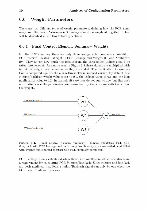
For the FCE summary there are only three configurable parameters: Weight HFCE Stiction Backlash, Weight H FCE Leakage and Weight H Loop Nonlinear-ity. They adjust how much the results from the thresholded indices should betaken into account. As can be seen in Figure 6.4 these signals are multiplied withindividual weight parameters before they are added. The result after the summa-tion is compared against the alarm thresholds mentioned earlier. By default, thestiction/backlash weight value is set to 0.9, the leakage value to 0.1 and the loopnonlinearity value to 0.2. In the default case they do not sum to one, but this doesnot matter since the parameters are normalized by the software with the sum ofthe weights.

Figure 6.4. Final Control Element Summary. Indices calculating FCE Stic-tion/Backlash, FCE Leakage and FCE Loop Nonlinearity are thresholded, multipliedwith weights and summed together to a FCE summary parameter.

FCE Leakage is only calculated when there is no oscillation, while oscillations area requirement for calculating FCE Stiction/Backlash. Since stiction and backlashare both nonlinearities, FCE Stiction/Backlash signal can only be one when theFCE Loop Nonlinearity is one.

6.6 Weight Parameters 31

Consider the case when the leakage signal is one (indicating leakage) and theother signals are zero. With the default weights this would result in FCESUM =(0 · 0.9 + 0 · 0.2 + 1 · 0.1)/(0.1 + 0.2 + 0.9) = 0.083. Even if no filtering (see Section6.8 for details) is used, the FCE SUM would never be able to exceed any alarmseverity threshold (0.2/0.4/0.6/0.8). Thus, this kind of error would not even resultin an alarm on the lowest severity level.

For the stiction case the result would be FCESUM = (1 ·0.9+1 ·0.2+0 ·0.1)/(0.1+0.2 + 0.9) = 0.92. This means that in case of stiction it would be possible to reachall severity levels. If there is some nonlinearity but no stiction in the process FCESUM would be 0.17 which would not exceed any severity levels.

As seen above, the default FCE weight parameters are not satisfactory since thereis no possibility to detect leakage or nonlinearities unless they are combined.Therefore a change of the default threshold or the alarm severity levels shouldbe considered. It should also be mentioned that the index naming is not consis-tent today. To follow the standard Weight H Loop Nonlinearity should be renamedto Weight H FCE Loop Nonlinearity in order to follow the convention.

If the software for some reason is unable to calculate one of the preconditions, itwill still affect the result since it is taken into account in the normalization. Thisproblem appears also in the Loop Performance Summary and will therefore bediscussed in further detail in Chapter 11.

6.6.2 Loop Performance Summary Weights

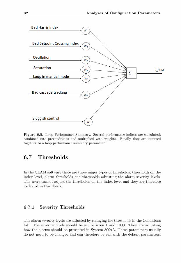
There are seven different weights for the Loop Performance Summary, one forevery precondition. The fusion of thresholded indices is more complicated than inthe Final Control Element Summary, see Figure 6.5.

In this case the default alarm severity levels are 0.1, 0.2, 0.3 and 0.4. Also inthis setup there are some preconditions that can never give rise to any alarm bythemselves. For example, independent of filtering the preconditions bad cascade

tracing and sluggish control are both unable to give rise to any alarms without helpfrom other preconditions, since not even the lowest threshold can be exceeded.

If filtering is used, the 0.1 weighted preconditions in Figure 6.5 will all convergeto 0.1, but they will never exceed the threshold and thereby never give rise to anyalarm. Thus, with the default configuration only two of seven preconditions canseparately result in an alarm. Therefore it might be a good idea to reconsider thedefault Loop Performance Summary weights.

As mentioned in the FCE part before, preconditions that for some reason have notbeen calculated would still affect the result as a consequence of the normalization.


Figure 6.5. Loop Performance Summary. Several performance indices are calculated,combined into preconditions and multiplied with weights. Finally they are summedtogether to a loop performance summary parameter.

6.7 Thresholds

In the CLAM software there are three major types of thresholds; thresholds on theindex level, alarm thresholds and thresholds adjusting the alarm severity levels.The users cannot adjust the thresholds on the index level and they are thereforeexcluded in this thesis.

6.7.1 Severity Thresholds

The alarm severity levels are adjusted by changing the thresholds in the Conditionstab. The severity levels should be set between 1 and 1000. They are adjustinghow the alarms should be presented in System 800xA. These parameters usuallydo not need to be changed and can therefore be run with the default parameters.

6.8 Filter Parameters 33

Table 6.1. Default alarm thresholds for Final Control Element Summary and LoopPerformance Summary.

Threshold FCE Critical 0.8Threshold FCE Severe 0.6Threshold FCE Warning 0.4Threshold FCE Moderate 0.2Threshold LPS Critical 0.4Threshold LPS Severe 0.3Threshold LPS Warning 0.2Threshold LPS Moderate 0.1

6.7.2 Alarm Thresholds

In CLAM there are four alarm thresholds for the final control element summaryand four thresholds for the loop performance summary. They are divided intomoderate, warning, severe and critical.

As mentioned before, the different indices are thresholded and then weighted to-gether. The weighting results in a value between zero and one, where one meansthat a threshold is exceeded and zero that it is not. By default these values are setas presented in Table 6.1 below. As an alternative to changing these thresholds,the weight parameters can be modified.

6.8 Filter Parameters

There are two configuration parameters with a prefix of ”filter” (not W as it says inthe system 800xA configuration guide), one filter parameter for the Final ControlElement Summary and one for the Loop Performance Summary. They both workin the same manner, performing low-pass filtering to adjust how much the resultfrom the last CLAM execution should be taken into account compared to the priorones. The filtering is performed using exponential moving average. The filteredvalue Dout represents the diagnostic parameter that is shown in the CLAM mainfaceplate and is calculated as Dout(t) = f ·D(t) + (1− f) ·Dout(t− 1), where f isthe filter parameter and D represents the latest calculated diagnostic summary.

By default, the filter parameters are set to 0.5. According to the staff at SodraCell Morrum the CLAM alarm list is checked once a day, usually in the afternoon.To avoid facing a huge amount of alarms they do not want alarm upgrades witha higher frequency than once a day. Since the aim with their use of CLAM isto discover changes in the dynamics that often happens slowly over a long periodof time, it does not matter if it takes a few days before the alarms exceed thethresholds and become visible in the alarm list.


Of course the configuration of the filter parameters depends on the choice of theData Set Size and Data Interval. A short data sequence and a large filter valuewould make the diagnosis sensitive to temporary disturbances. In the same way alow value on the Data Interval CLAM would calculate new diagnoses more oftenand thereby making changes visible in the alarm list very fast. Consequently, alarger execution interval and a rather long data sequence allow a larger filter valuewithout being sensitive to temporary disturbances.

Compared to the alarm thresholds, in the loop performance summary case, analarm on the lowest level (moderate) requires a value larger than 0.1 to be regis-tered. The other severity levels are 0.2, 0.3 and 0.4.

In order to determine a suitable filter value, diagnosis values of 0.11 and 0.5 werecompared. In Figure 6.6, Figure 6.7 and Figure 6.8 the alarm curves are plottedfor the filter values 0.1, 0.2 and 0.5 (default).

Figure 6.6. Loop performance summary alarm curve with filter parameter f=0.1. Herenew alarms for the severe error are not generated more than once in 24 hours (until thehighest level is reached), while it takes 176 hours for a small error to generate an alarm.

6.8 Filter Parameters 35

Figure 6.7. Loop performance summary alarm curve with filter parameter f=0.2. Herenew alarms for the severe error are generated more than once in 24 hours (until thehighest level is reached), while it takes only 78 hours for a small error to generate analarm.


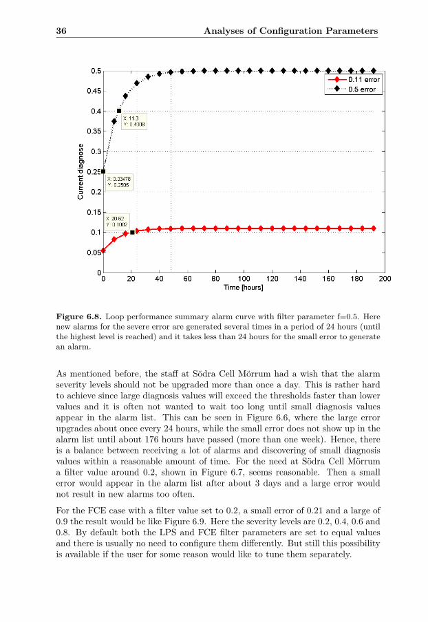
Figure 6.8. Loop performance summary alarm curve with filter parameter f=0.5. Herenew alarms for the severe error are generated several times in a period of 24 hours (untilthe highest level is reached) and it takes less than 24 hours for the small error to generatean alarm.

As mentioned before, the staff at Sodra Cell Morrum had a wish that the alarmseverity levels should not be upgraded more than once a day. This is rather hardto achieve since large diagnosis values will exceed the thresholds faster than lowervalues and it is often not wanted to wait too long until small diagnosis valuesappear in the alarm list. This can be seen in Figure 6.6, where the large errorupgrades about once every 24 hours, while the small error does not show up in thealarm list until about 176 hours have passed (more than one week). Hence, thereis a balance between receiving a lot of alarms and discovering of small diagnosisvalues within a reasonable amount of time. For the need at Sodra Cell Morruma filter value around 0.2, shown in Figure 6.7, seems reasonable. Then a smallerror would appear in the alarm list after about 3 days and a large error wouldnot result in new alarms too often.

For the FCE case with a filter value set to 0.2, a small error of 0.21 and a large of0.9 the result would be like Figure 6.9. Here the severity levels are 0.2, 0.4, 0.6 and0.8. By default both the LPS and FCE filter parameters are set to equal valuesand there is usually no need to configure them differently. But still this possibilityis available if the user for some reason would like to tune them separately.

6.9 Dead Time 37

The description in the system 800xA configuration guide about these parametersis not updated and needs to be rewritten.

Figure 6.9. Final Control Element summary alarm curve with filter parameter f=0.2.Here new alarms for the severe error are not generated more than once in 24 hours (untilthe highest level is reached), while it takes 80 hours for a small error to generate analarm.

6.9 Dead Time

In CLAM, there is a configuration parameter called dead time that representsthe time it takes until a change in the controller output is visible in the processvalue. It affects Harris index and ACF ratio index and is by default set to thevalues shown in Table 6.4. At Sodra Cell Morrum the dead time is often welldocumented in their documentation system and therefore it is easy for the staff tocheck up the correct values.


In data collected at Sodra Cell Morrum, the dead time parameter is defined in 18out of 24 cases. To investigate how the indices are affected if CLAM is configuredwith the correct or default dead time, the algorithm for calculating Harris indexwas run three times, once with the RegDoc value (see Section 3.3), once with theRegDoc value + 20 % and once with the default value. The result is shown inTable 6.3. In all cases, there is a major difference between using the estimateddead time and the default one. It is very obvious that Harris index is affected bythe choice of dead time. A longer dead time gives a higher Harris index, i.e. lessimprovement potential.

Some of the loops exceed the thresholds and are marked with italic text. In 5 of 12cases (marked with bold text) the correct dead time results in a value below thethreshold (alarm) while the default value gives a value greater than the threshold(no alarm), resulting in missed detections. It can therefore be stated that thechoice of the dead time parameter is of great importance. In these particularexamples the default dead times were quite far from the correct ones.

To investigate how a smaller deviation would affect the result, the algorithm wasfed with 20 % larger values than the estimated ones. For most loops, this re-sulted in a small deviation or sometimes no deviation at all. For some loops, likeLC471640, the resulting deviation was quite big and led to missed detection.

Thus, the choice of the dead time parameter is of great importance for the result.A larger dead time than the real one gives an index value that allows worse control.A smaller dead time could result in false alarms. Since a small deviation from thecorrect value may result in a false alarm it is also important that the documenteddead time parameters are correct. Otherwise the result may be just as misleadingas in the case with the default parameters.

Since the dead times at Sodra Cell Morrum are often documented in RegDoc, somestatistics can be concluded. Unfortunately there is no simple way to get moreinformation about cascade mode and more details about the loop type than whichmajor category it belongs to. Therefore, these statistics are not quite comparablewith the default values in Table 6.4. In Table 6.2 some statistics are presentedand histograms are provided in Appendix D.

6.9 Dead Time 39

The dead times at Sodra Cell Morrum differ quite a lot from the default values.Most values are smaller than the default values and the result from Harris indexmay thereby allow worse control, but as seen by looking at the column max in Table6.2, there are at least one flow loop and one temperature loop that may cause falsealarms. This motivates the use of estimated dead times instead of default values.It is also an indication that the default values should be reconsidered when usingthem in a process industry like Sodra Cell Morrum, where the dead times differ.On the other hand, it would be even worse to use these dead times from SodraCell Morrum in an industry with larger dead time, since this would result in falsealarms.

Table 6.2. Dead time statistics from Sodra Cell Morrum.

Average min max median # Documented (# Total)Flow 2.45 0 45 1.73 224 (584)Level 36.74 0 1000 1.6 79 (275)Pressure 2.88 0 26 1.6 47 (239)Composition 44.11 0.4 193 29.5 38 (70)Temperature 70.58 7 411 21 42 (213)


Table6.3.

Harris

indexfor

differentdead

times.

Loop

FC471614

FC482215

FC542024

FC452003

FC490106

FC471609

FC471010

LC542015

LC482201

LC482122

LC471640

TC482017

QC542030

QC542018

QC542002

QC482213

QC472404

QC471619

Default

1010

1010

1010

10100

100100

200200

10050

50100

50100

deadtim

eEstim

ated1.3

3.81.5

4.41.1

23.6

4350

105

13151

9.517

211.2

36dead

time

Harris

index0.68

0.710.3

70.3

30.4

0.730.84

0.720.0

90.0

20.99

0.951

0.990.98

0.940.86

0.94defaultH

arrisindex

0.3

40.61

0.2

70.3

30.2

80.64

0.5

60.5

20.0

30

0.540.7

10.96

0.940.89

0.1

10.78

estimated

+20%

Harris

index0.3

40.61

0.2

70.1

90.2

80.64

0.5

60.4

80.0

30

0.2

90.64

10.8

0.830.83

0.1

10.72

estimated

Difference

0.340.1

0.10.14

0.120.09

0.280.24

0.060.02

0.70.31

00.19

0.150.11

0.750.22

default-estim

ated

6.10 Loop Category 41

6.10 Loop Category

The parameter Loop Category decides what indices that should be calculated andthe choice of default dead time for Harris index. The default dead time is differentfor different loop types and cascade modes can be seen in Table 6.4.

Table 6.4. Default dead time (in seconds) for different loop categories used in CLAM.

Flowliquid

Flowother

Temperature

Com

position

Pressure

Leveltight

Levelaverage

otherSRP

otherINT

Master 30 30 200 30 100 100 200 100 100slave/single 10 30 100 10 50 50 100 50 50

There are several different loop categories:

• Flow liquid: loop with a flow of liquid.

• Flow other: loop with a flow that is not liquid. Typical examples: gas orsteam. In this case there is no difference between the dead times for masteror slave/single alternatives.

• Temperature: loop controlling temperature, often resulting in slower dynam-ics.

• Composition: loop controlling a composition, for example chemical mixing.

• Pressure: loop controlling pressure.

• Level tight: level control loop where it is important to keep a steady level.

• Level average: loop with more loose level control like buffers, etc.

• otherSRP: other self regulating loops.

• otherINT: other integrating loops.


6.11 Resample Interval

The parameter Resample interval decides the interval of the received data fromthe history log. If this parameter is set to the same value as the logging interval,CLAM will collect values with the same interval. If it is set to a lower value, somepoints in the log will be excluded and a higher value would result in a sequencewith a tighter interval than the log. This means that these extra points come frominterpolations between the correct points.

Since the data should be used for making diagnoses about the control loop per-formance we want to use data as close to the real data as possible. Therefore thisparameter should be set to the same value as the logging interval.

6.12 Aggregate Function

This function is used as an input in a function call for collecting data from thelog. By default this parameter is set to 1, meaning that interpolation will be usedif some logged data is flagged to be bad. This value can be changed to a largenumber of different aggregates that would perform operations on the data beforeit is used in CLAM. One such aggregate is time average that returns a single valueinstead of a sequence of samples. If this aggregate is used, there is no possibilityfor CLAM to calculate any diagnoses. Therefore, this is a parameter that shoulddefinitely not be possible to modify for an ordinary user.

6.13 Inhibit Value

To save resources there is a Boolean parameter called Inhibit value decidingwhether a CLAM analysis should be executed during a production stop. By de-fault this parameter is set to TRUE, meaning that CLAM will not calculate newdiagnoses when the inhibit input signal is true.

Chapter 7

History Logging

In this chapter, analyses and results regarding the effects on CLAM due to thehistory log setup are presented. First, the risks of using the OPC direct loggingapproach are analyzed. This is followed by an analysis of how CLAM is affectedby the choice of logging setup and logging interval. Finally, a discussion about thesize of the history log is presented.

7.1 OPC Direct Logging with 3 Seconds CyclicRate

In order to store a new value in the history log each value has to be transferred overthe network (MB300). Since the network originates from the 1980s its capacityis quite limited. The cyclic rate might be 1, 3 or 9 seconds, where 9 seconds isrecommended due to performance. Since this is a quite slow sample rate with alarger risk of aliasing, a cyclic rate of 3 seconds is assumed in this analysis.

Using a logging interval of 5 seconds (like Sodra Cell Morrum) and by assumingthat the starting time is the same, the actual logging procedure would be likeFigure 7.1 (assuming that the time for data transfer is neglected). Since 5 is not amultiple of 3, the logging interval cannot be constant. This means that even if weconfigure the log to save a value at the timestamps 0/5/10/15/20/25 the actualsamples saved at these points will correspond to the timestamps 0/3/9/15/18/24.The saved samples might be up to two samples old, for example the sample savedat timestamp 5 in the log sequence (C), corresponds to sample 3 in the controllersequence (A), see Figure 7.1.

43

44 History Logging

Figure 7.1. Synched data transfer from the controller (A), via the network (B) to historylog (C) using OPC direct logging with 3s cyclic rate. Due to the network limitations thesamples logged with timestamps 0/5/10/15/20 actually originate from the timestamps0/3/6/15/18, i.e. the time between the samples in the log is not constant.

By assuming that the times for execution are not synchronized, the logged samplesmight be up to 4 samples old. This can be seen Figure 7.2, where the sample savedat timestamp 10 in the log (C) corresponds to sample 6 in the controller sequence(A). The problem would get even worse by assuming that the cycle time in one ormore of these cases is drifting. So it is clearly a fact that the data sequences inthe log might be quite far from the original one in the controller.

Figure 7.2. Unsynched data transfer from the controller (A), via the network (B) tohistory log (C)using OPC direct logging with 3s cyclic rate without time synchronization.This means that the logged samples might correspond to samples that are up to fourseconds old.

7.1 OPC Direct Logging with 3 Seconds Cyclic Rate 45

In order to see what happens when a signal is logged, a simple example usinga noise-free sinusoid was investigated. As seen before, the sampling interval inthe log is irregular with a maximum time difference of 6 seconds, i.e. a samplingfrequency fs of 1/6 Hz. To avoid aliasing let us use a sinusoid with a frequency off < fs/2 as recommended from the sampling theorem (Glad & Ljung, 2006). Witha sampling frequency of 1/6 Hz this gives a sinusoid with f < 1/12. In Figure 7.3below, the sinusoid sin(t/12) is shown together with the network collection points,i.e. f = 1/(2π · 12).

Figure 7.3. Sampled sinusoid. This is a simple sinusoid (line) sampled with a samplingfrequency of 3 seconds (diamonds).

Since the sample interval is not regular some sections will be not be used as seenin Figure 7.4.

46 History Logging

Figure 7.4. Network buffer vs. logged sample points. The diamonds represent thesamples stored in the log. It is clear that the logging frequency is not constant.

Now comparing the original signal with the logged one, it can be seen that thelogged signal differs a little bit from the other, see Figure 7.5. How this will affectthe result from index calculations will be analyzed in Section 7.2.

7.1 OPC Direct Logging with 3 Seconds Cyclic Rate 47

Figure 7.5. Comparison between logged and original sinusoid. It is clear that the loggedsignal differs from the original signal.

But what happens when the signal is oscillating with a higher frequency? Simplyby looking at faster sinusoids like the ones in Figure 7.6, it is easy to realize thatthe logging procedure now has destroyed a lot of the information in the originalsignals. This is a typical example of aliasing.

48 History Logging

(a) sin(t/2)

(b) sin(3t/2)

Figure 7.6. Sinusoids destroyed by aliasing. The aliasing gets worse as the distancebetween the logged samples increase.

7.2 Effects on CLAM Results 49

7.2 Effects on CLAM Results

In industries where control equipment like AC450 and MB300 are used, a commoninterval of execution is once every second. This setup is standard at Sodra CellMorrum. They have a history log configured to log samples with an interval of 5seconds using the TTD approach.

To investigate how it looks in reality, a liquid flow loop from Sodra Cell Morrumwas used. The data in the log is sampled with an interval of 5 seconds comparedto the data collected directly from the controller, sampled with an interval of 0.5seconds.

With the setup in Morrum with System 800xA, AC450 and MB300 there is notime synchronization between the log in 800xA and the Easyview 0.5s log feature,meaning that we do not know if a timestamp from Easyview really is from thesame point of time as the corresponding timestamp in the history log. To eliminatepotential problems all data sequences in the result analysis are based on datadownsampled from the Easyview log.

To see how the index calculations are affected by different sampling intervals, allindices were evaluated for datasets with an interval of 0.5, 3, 5, 6 seconds and witha varying interval similar to OPC direct Logging with 3 seconds cyclic rate. Theresults can be seen in Appendix C.

Since the number of analyzable loops is so few, there is no possibility to obtainany statistically motivated conclusions, but some indications can be seen.

First, it can be concluded that OPC Direct Logging with cyclic subscription witha cyclic rate of 3 seconds, in combination with a 5 second history log, is notrecommended from a monitoring perspective. Many indices seem to be unaffected,but some are clearly affected by the varying sampling interval. An example is thestandard deviation of the control output (index #5) that for FC542119 becomesabout twice as large (5.58) as the sequences with constant sampling interval (2.77).For FC542119 it is also clear that the Skewness and Kurtosis errors (index #6 and#7) both increase with about a factor 10.

For FC542114 an observation is that Nonlinearity index 2 (index #34) and Non-Gaussianity index (index #35) both become a lot smaller than for the originalsignal.

Which indices that are affected and how much seems to differ quite a lot betweendifferent loops. Since this is unknown for a CLAM user the recommendation mustnot be to use logged data with varying sampling interval for monitoring purposes.

50 History Logging

By looking at the intervals 0.5/3/5/6 seconds it can be seen that some indices areaffected already when data is down-sampled to a 3 s interval. As expected mostindices seem to be less affected when the logged sample interval is closer to thereal interval. This is once again a motivation why the down-sampling should beavoided when possible or at least minimized if down-sampling is necessary.

In all cases Harris index seems to be overly optimistic when the indices are eval-uated for larger sampling interval, i.e. saying that there are no problems even ifthere are. This means a risk for missed detections when the original index valuemight result in an exceeded threshold while the others do not indicate any problem.Another interesting observation is that the compression factor decreases when thesampling interval is increased.

It can also be seen that the Setpoint Crossing index seems to increase in a way thatcorresponds to the ratio between the sampling intervals. Comparing the 3s and5s results with the original 0.5s results the values increase with an approximatefactor 6 and 10 respectively. A possible explanation for this is that when data isdown-sampled the number of zero crossings seems to remain, while the number ofdata points on different sides of zero decrease. This results in a changed relationbetween the number of zero crossings and the number of samples.

If the original signals contain high frequency components or fast changes, a slowlog configuration will modify the signals. Then the logged data is unsuitablefor monitoring algorithms. No matter how intelligent the loop asset monitoringalgoritms are, they will not be able to diagnose the loop since the data sequenceis completely different compared to the original sequence. The data simply hasto be logged with a higher sample rate to be useful. Some indices seem to beaffected by the different sampling intervals and may lead to false alarms or misseddetections. At Sodra Cell Morrum this does not seem to be a problem since mostsignals change rather slowly.

Ideally, the monitoring algorithms should be applied to a data sequence that hasnot been down-sampled. This is not possible at Sodra Cell Morrum today since afaster logging would increase the system load on the AC450 equipment togetherwith increased network load. If the performance of the controller and networkwould increase and allow faster logging it would be welcome from a monitoringperspective.

7.3 Size Analyses of History Log

By investigating the history log at Sodra Cell Morrum it can be stated that ap-proximately 24 bytes are needed to store one value for one signal. This meansthat 24 · 3600/5 = 17280 bytes are needed to store a signal for one hour using 5slogging interval. At Sodra Cell Morrum there are approximately 1200 loops andlogging of at least PV, SP and CO is required. Thus, about 7200 MB are neededfor the history logging today.

7.3 Size Analyses of History Log 51

Since a history log with different density is not wanted from a monitoring perspec-tive and because it sometimes could be interesting to see older logged signals thantoday, the need of space for storing data for one year was analyzed. Simply bymultiplying 17280 bytes with the number of signals to be logged (3600) and thenumber of hours in one year (8760) it turns out that about 507 GB are neededto store a year of data. Today the cost of a hard drive with such capacity canbe considered to be quite small compared to the revenue at Sodra Cell Morrum.Therefore a upgrade of the logging capacity might be reasonable.

Chapter 8

Validation of Results fromCLAM

In this chapter the result from CLAM analyses made on a number of control loopsat Sodra Cell Morrum are validated. From their point of view, false alarms areoften unacceptable since it may lead to unnecessary maintenance and thereby un-necessary costs. Therefore, detailed analyses of control loops indicating problemswere performed. At this time, 4 loops indicated problems; one pressure controlloop (PC451029), two level control loops (LC471640 and LC482122) and one flowcontrol loop (FC442064).

To make sure that CLAM does not miss any obvious problems, plots of all mon-itored loop were also inspected manually. A flow control loop (FC542024), witha rectangular PV signal was found and a detailed analysis is presented in thissection.

8.1 PC451029

For the pressure control loop PC451029 CLAM indicated rather severe problems.The result of the loop performance summary was 0.3 and the FCE Summary was0.17. This means that the loop performance summary was equal to the third alarmseverity threshold, while FCE summary did not exceed the first threshold (0.2).

53

54 Validation of Results from CLAM

At the index level the following indices exceeded their thresholds:

• Index #2: Standard Deviation Loop Error (Normalized)

• Index #14: Saturation Index

• Index #16: Auto-correlation Ratio

• Index #17: Setpoint Crossing Index

• Index #20: Harris Index

• Index #32: Valve sizing index

• Index #34: Non-linear 2nd Index

By looking at a plot (Figure 8.1) of the analyzed signals, it can be concluded thatthis loop is malfunctioning. The PV signal shows no sign of getting smaller as theCO signal is set to zero. The PV signal is actually never close to the SP signalat all. According to the staff at Sodra Cell Morrum, the PV signal cannot bedecreased due to too high surrounding pressure. This problem originates from theprocess layout in this section of the plant and cannot be solved unless the layoutis changed.

According to the results at the index level and the plot of PV, SP and CO, theresult from CLAM seems reasonable, but it can be discussed if also the FCESummary should result in an alarm.

8.1 PC451029 55

0 500 1000 1500 2000 2500 3000 3500 4000 4500 500035

40

45

50

55

60PC451029

Samples [1 sample = 5s]

Sign

al ra

nge

[%]

PVSP

0 500 1000 1500 2000 2500 3000 3500 4000 4500 50000

0.1

0.2

0.3

0.4


Sign

al ra

nge

[%]

CO

Figure 8.1. Plot for the pressure control loop PC451029. Due to too high surroundingpressure the PV signal cannot be decreased even if CO is zero.


8.2 LC471640

The CLAM analysis for the level control loop LC471640 resulted in a loop per-formance summary set to 0.4, i.e. equal to the highest alarm severity threshold.This high value originates from detected oscillations at the index level. By lookingat a plot of the analyzed data it can be seen that there is no doubt that PV isoscillating, see Figure 8.2. On the other hand, this is a controller for a buffer tank,where one of its tasks is to remove oscillations in the system. Therefore this loopshould be allowed to oscillate rather much without generating any alarms, at leastnot on such high severity level.

Today there is no way to decide whether alarms should be generated based on theseverity of the oscillation. CLAM only detects whether there is an oscillation ornot. For level loops like this one, it might be desirable to have a parameter wherethe user can specify how large oscillation amplitude that is acceptable before analarm should be generated or not. For this loop the conclusion is that it is correctthat CLAM detects oscillations, but some functionality for tuning the tolerance ofoscillations might be desired by some users, at least for level loops.

0 100 200 300 400 500 600 700 800 900 10000.1

0.2

0.3

0.4

0.5LC471640


Sign

al ra

nge

[%]

0 100 200 300 400 500 600 700 800 900 100020

30

40

50


Sign

al ra

nge

[%]

CO

PVSP

Figure 8.2. Plot for the level control loop LC471640. The PV signal is clearly oscillating.

8.3 LC482122 57

8.3 LC482122

The result of the CLAM analysis of the level control loop LC482122 was similar toLC471640 mentioned before. Since an oscillation was detected at the index level,the loop performance summary parameter is assigned with the value 0.4, i.e. equalto the threshold of the highest alarm severity level.

By looking at a plot of the analyzed data, it can be concluded that an oscillationdefinitely is present, see Figure 31. The problem whether oscillations always shouldgenerate alarms for level loops is also similar to the case with LC471640 mentionedbefore.

0 500 1000 1500 2000 2500 3000 3500 4000 4500 50000.62

0.64

0.66

0.68

0.7LC482122


Sign

al ra

nge

[%]

0 500 1000 1500 2000 2500 3000 3500 4000 4500 500050

55

60

65

70


Sign

al ra

nge

[%]

CO

PVSP

Figure 8.3. Plot of the level control loop LC482122. The PV signal oscillates with lowfrequency.


8.4 FC542024

The flow control loop FC542024 caught the attention during a manual analysis ofall loops that were monitored by CLAM at Sodra Cell Morrum. In this case, theSP signal is varying; PV has a rectangular shape and CO triangular, see Figure8.4. According to the CLAM result there were no indications of exceeded indexthresholds. The oscillation was not detected due to the small amplitude.

In order to see if the oscillations in the PV signal were caused by using a toolarge dead band, the loop was monitored at the same time as the dead band wasdecreased. This resulted in an improved ability to follow the SP signal and adecreased oscillation, see Figure 8.5. It can also be seen that the CO signal doesnot move as intensely as before, which is preferred since it leads to less mechanicalwear.

2500 2520 2540 2560 2580 2600 2620 2640 2660 2680 27000.086

0.088

0.09

0.092

0.094FC542024


Sign

al ra

nge

[%]

2500 2520 2540 2560 2580 2600 2620 2640 2660 2680 270021.5

22

22.5

23


Sign

al ra

nge

[%]

PVSP

CO

Figure 8.4. Detailed plot for the flow control loop FC542024. The SP signal is varying;PV oscillates and is rectangular shaped and CO is triangular shaped.

8.4 FC542024 59

4600 4650 4700 4750 4800 4850 4900 4950 50000.2360.238

0.240.2420.2440.2460.248

FC542024


Sign

al ra

nge

[%]

4600 4650 4700 4750 4800 4850 4900 4950 500032

32.5

33

33.5


Sign

al ra

nge

[%]

PVSP

CO

Decreased Dead band

Decreased dead band

Figure 8.5. Detailed plot for FC542024. The dead band is decreased at sample 4800and the control performance is improved and the oscillation decreased.


8.5 FC442064

In CLAM analyses from Sodra Cell Morrum the following indications were foundfor the flow control loop FC442064:

• FCE Stiction/Backlash

• Loop Nonlinearity

• Data Reliability

• Harris Index

• Setpoint Crossing Index

• Oscillation Index

CLAM was at the time of the execution configured to use a data set size of 5000samples and a dead time based on information from RegDoc. To be able to makea more detailed analysis at the index level, a data sequence of 5000 samples werecollected from the history log. The result at the index level showed exceededthresholds for loop nonlinearity, data reliability and Harris index, but not for stic-tion/backlash, setpoint crossing or oscillation. The results can be seen in AppendixE.

By looking at a plot of the analyzed data, it can be seen that the PV signal isclearly oscillating (see Figure 8.6), i.e. the performance indices should at least giveindications of this. The oscillation index on the control error (index #21) actuallyfailed to detect any oscillation at all, i.e. not even an oscillation with amplitudesmaller than the specified thresholds was found. The oscillation amplitude of thePV signal is about the same for the whole sequence, except for a section betweensample 2000-2600, where it is larger. To see whether this deviating part may haveaffected the result, all indices were calculated for different sequences taken fromthe sequence of 5000 samples.

8.5 FC442064 61

Figure 8.6. Data sequence for FC442064 used for validating the CLAM result. Thesequence oscillate with a rather constant amplitude except for a few peaks in the middle.

For the sections 0-2000 and 3000-5000 oscillations were detected and both thestiction correlation index and stiction histogram index indicated stiction/backlash.In the sequence 1500-3500 oscillations were detected, but there was no sign ofstiction.

It is hard to draw any conclusions whether the result from CLAM for this loopis reasonable or not. This is due to the fact that the data sequences evaluatedonline and offline are not identical. The result from the index level compared tothe data plot indicates no signs of false alarms. There is no doubt that the PVsignal is oscillating and by looking at a more detailed plot in a sequence wherestiction/backlash is detected (see Figure 8.7) this indication from CLAM can bestated to be reasonable. This interpretation is also confirmed by the staff at SodraCell Morrum, where they concluded that maintenance should be planned for thevalve used in this loop.

Thus, it seems like indications from CLAM can be trusted, but depending onthe data sequence there might be times when CLAM cannot detect all problems.Internally in CLAM, a prerequisite to the calculation of the stiction indices is thatthe PV signal is oscillating. Therefore it is crucial that oscillations really can bedetected. A temporary solution might be to use a smaller data set size and in thisway decrease the risk of missed detection due to the quality of the data.


Figure 8.7. Detailed plot of FC442064 with characteristic stiction/backlash look. ThePV signal is rather rectangular and the CO signal is triangular.

The disadvantages in this case are that slow oscillations cannot be detected andthat CLAM has to be executed more often if the system always should be moni-tored. For a more lasting solution, the algorithms for detecting oscillations prob-ably need to be reviewed.

In the interval 1500-3500, it can be seen that the characteristic stiction/backlashbehaviour here is disturbed by three sections were the PV signal oscillates quite alot, see Figure 8.8. This may explain why CLAM is unable to detect the stiction.

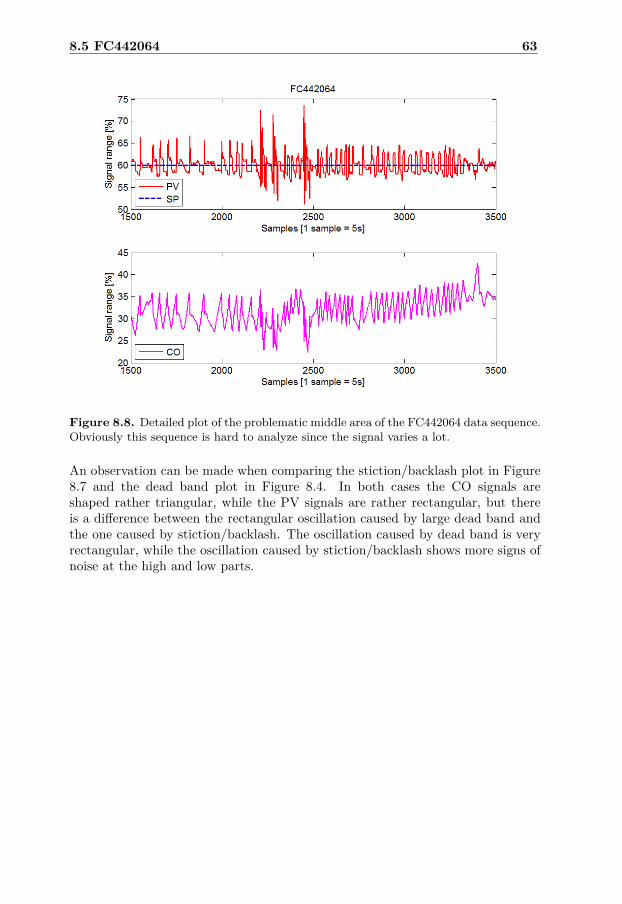
8.5 FC442064 63

Figure 8.8. Detailed plot of the problematic middle area of the FC442064 data sequence.Obviously this sequence is hard to analyze since the signal varies a lot.

An observation can be made when comparing the stiction/backlash plot in Figure8.7 and the dead band plot in Figure 8.4. In both cases the CO signals areshaped rather triangular, while the PV signals are rather rectangular, but thereis a difference between the rectangular oscillation caused by large dead band andthe one caused by stiction/backlash. The oscillation caused by dead band is veryrectangular, while the oscillation caused by stiction/backlash shows more signs ofnoise at the high and low parts.

Chapter 9

Online Help

In order to make CLAM easier to use and to eliminate problems related to incorrectconfigurations, the results and conclusions from this thesis have been formulatedinto guidelines. These guidelines have been documented in an online help file, i.e.a chm-file. Since System 800xA and CLAM already are supporting chm-files, onlya small configuration procedure is needed to connect CLAM to this help file. Thismeans that whenever a user needs to read the online help, it is only a F1-clickaway.

In this thesis a prototype of an Online Help has been made. This prototype hasbeen tested successfully at Sodra Cell Morrum and will be sent to ABB in Indiafor implementation of an official release.

9.1 Outline of the Online Help

The help file is divided into three major parts:

• CLAM Configuration: includes detailed instructions for how CLAM shouldbe configured in order to generate reliable diagnoses.

• Configuration Parameters: detailed information about all relevant configu-ration parameters including recommended default values.

• Interpretation of results: includes instructions for how results from CLAMcan be interpreted and detailed information about common diagnoses.

65

Chapter 10

Conclusions

In this thesis it has been analyzed how CLAM should be configured in order togenerate reliable diagnoses. All relevant configuration parameters were analyzedin detail and the configuration approach was evaluated together with the staff atSodra Cell Morrum. It has been concluded that some of the recommendationsand default values should not be used and that some parts of the configurationprocedure should be modified.

These results have been documented in an online help. It has been tested success-fully at Sodra Cell Morrum and will be sent to ABB in India to be modified andredesigned to an official release.

The results from CLAM have been concluded to be reasonable when CLAM isconfigured according to the conclusions in this thesis. In one case, CLAM wasunable to detect oscillations due to the large variations in the data sequence, butall cases where CLAM indicates problems have been stated to be reasonable.

In the following sections, summaries of the result and conclusions from the chaptersbefore are given. Suggestions of future work are given in Chapter 12.

10.1 Configuration Parameters

It was found that several of the recommendations and default values described inthe configuration guide need to be updated. Some of them should be modified andsome are incorrect.

When configuring the data set size and data interval it has to be considered thatsome combinations may lead to gaps where the performance of the system is notmonitored. A recommendation is to set the data interval equal to the data set sizemultiplied with the sample interval in the history log. It was also concluded thatusing a small data set size means that slow oscillations cannot be detected.

67

68 Conclusions

The cascade mode configuration approach used today is confusing for the userssince there are no clear alternative to choose for single loops.

The weights and alarm thresholds used today for the final control element summaryand loop performance summary means that some problems cannot give rise to anyalarm at all. In the final control element summary case only stiction/backlash willresult in an alarm.

The default filters used today with f=0.5 means that several alarms per loop maybe generated in one day. Since this is often not wanted by the users the filterparameter f should be decreased to 0.2.

The result from Harris index was shown to be very sensitive to the choice ofdead time. At Sodra Cell Morrum, the dead times overall are smaller than thedefault values, meaning that the result from Harris index should not be trustedwhen the default values are used. Therefore it should be considered to implementfunctionality for informing the users when the result from Harris index is notreliable.

The possibility to change the aggregate function parameter should be removedsince a change of this parameter will affect the CLAM analyses.

10.2 History Logging

It was found that the closer the logging interval is to the execution interval, themore reliable are the results from CLAM. Using the OPC direct logging with alogging interval that is not a multiple of the cyclic rate is not recommended forperformance monitoring. It results in a logging interval that is not constant anda logged signal that might be completely different from the original.

The TTD logging approach used at Sodra Cell Morrum has been concluded towork for the needs of CLAM. The logged signals do not differ from the originalsignals as much as the results of the index calculations are affected.

Today the history log at Sodra Cell Morrum is divided into three parts withdifferent density in order to save storage space. According to the current size, itshould be possible and not especially expensive to change the log setup to a logwith a constant density. It would then also be possible to save data for a longerperiod of time.

10.3 Validation of Results from CLAM 69

10.3 Validation of Results from CLAM

It has been concluded that the indications and results from CLAM are reasonableand can be trusted. The users do not have to worry about false alarms, but theremight be times when CLAM is unable to detect problems. One such example wasseen in Figure 8.8, where CLAM was unable to detect the oscillations due to thevarying oscillation amplitude. This also revealed a disadvantage of using a data setsize of 5000 samples, since a small section of data with high variance may removethe possibility of detecting oscillations. Therefore, unless the oscillation detectionindices are reviewed, it would be motivated to use a smaller data set size.

It was concluded together with the staff at Sodra Cell Morrum that there is nopossibility to adjust the tolerance of oscillations in buffer tanks. Even if they areallowed to oscillate within certain limits CLAM will still generate an alarm if theoscillation exceeds the standard thresholds.

Chapter 11

Future Work

As described in this thesis there are a number of issues regarding CLAM that canbe improved, both in the user guides and the implementation of CLAM. Some ofthese are urgent and some can be considered when all the prioritized problems aresolved.

The most urgent issue is the possibility to modify the parameter Aggregate func-tion. This possibility should be removed since a change here would affect theresults from CLAM totally. Another prioritized action is to change the recom-mendation in the user guide regarding the parameter PV high. This is importantsince it affects a lot of performance indices and how sensitive they should be.

As mentioned in Chapter 9, the online help produced during this project is notready to be shipped to the customers, since it needs to be redesigned in line withthe online help for System 800xA. The text in this file is already written andtherefore the amount of time needed for producing a final version should be small.

As mentioned before, some of the preconditions are unable to exceed severitythresholds and inactive indices affect the result via the normalization. Therefore,alternative solutions should be investigated. It would be interesting to remove thethresholding used today and find a solution where the strength of the indices iskept through the summary step. This way, it would for example be possible togenerate alarms on different severity levels for oscillations based on the oscillationamplitude. In order to do this, it is probably easiest to modify all performanceindices so the all return their result in the same interval.

71

Bibliography

ABB. (2011-01-24). Horch, Alexander. Phone meeting.

ABB. (2003a). Loop Performance Manager 3.0 User Manual.

ABB. (2003b). Success Story Sodra Cell Morrum - Speeding up productivity.Document id: 3BSE035148R0001

ABB. (2008). System 800xA - Extended Automation System Overview.

Document id: 3BUS092082

ABB. (2010a). System 800xA Asset Optimization 5.1 Configuration.

Document id: 3BUA000118-510

ABB. (2010b). System 800xA Asset Optimization 5.1 Operation.

Document id: 3BUA000150-510

ABB. (2008). System 800xA for Advant Master Configuration.

Document id: 3BSE030340R5021

ABB. (2011, January). System 800xA topologies. (internal presentation).Christian Johansson.

Bjorklund, S., Ljung, L. (2003). A Review of Time-Delay Estimation Techniques.42nd IEEE Conference on Decision and Control, Maui Hawaii, USA.

Choudhury, M. A. A. S., Shah, S. L. and Thornhill, N. F. (2004).Diagnosis of Poor Control Loop Performance using Higher Order Statistics.Automatica Vol 40, Pages 1719-1728.

Ender, E. (1993). Process Control Performance: Not as Good as You Think.Control Engineering Practice. Vol. 40, Issue 10, Pages 180-190.

Glad, T., & Ljung, L. (2006). Reglerteknik Grundlaggande Teori. Studentlitter-atur (in Swedish).

Harris, T. J. (1989). Assessment of Control Loop Performance.The Canadian Journal of Chemical Engineering, Vol 67, Issue 5, Pages 856-861.

73

Horch, A. (2000). Condition Monitoring of Control Loops (Ph.D. Thesis).Department of Signals, Sensors and Systems, Royal Institute of Technology,Stockholm, Sweden.

Horch, A. (1999). A Simple Method for Detection of Stiction in Process ControlLoops. Control Engineering Practice. Vol. 7, Issue 10, Pages 1221-1231.

Morrums Bruk. (2002). Morrums Bruk under 40 ar (in Swedish).

Schreiber, T. (1995). Efficient Neighbor Searching in Nonlinear Time SeriesAnalysis. International Journal of Bifurcation and Chaos. Vol. 5, Issue 2, Pages349-358.

Sodra Cell Morrum. (2010a). Andersson, Leif. Discussion.

Sodra Cell Morrum. (2010b). Andersson, Magnus. Discussion.

Sodra Cell Morrum. (2010c). Svensson, Gert. Discussion.

Sodra. (2004). Massans vag (in Swedish).

Sodra. (2008). Sodra Cell (in Swedish).

Thornhill, N. F., Hagglund, T. (1997). Detection and diagnosis of oscillation incontrol loops. Control Engineering Practice. Vol. 5, Issue 10, Pages 1343-1354.

Appendix A

Performance Indices

In this appendix, all performance indices used in CLAM are described.

75

APPENDIX A: PERFORMANCE INDICES Summary of Indices calculated by CLAM based on the LPM 3.0 User guide

# Name Description Index class 1 Mean Loop

E rror

Calculates the control error mean. Should be close to zero if no permanent off-set is present. Normalized to the interval [0-100 %].

Basic statistics

2 Standard

Deviation Loop

E rror

(Normalized)

Calculates the standard deviation of the normalized control error. Presented as [0-100 %]. Should be as small as possible, usually 1-5 %.

Basic statistics

3 Standard

Deviation Loop

E rror

(Engineering

units)

Same calculations as index 2, but in absolute engineering units. [min-max]. Should be small.

Basic statistics

4 Mean Process

Variable

The mean process value documents the actual operating point used during data collection (no performance index). The mean value can be used to analyze if certain control problems are related to certain operation points. [min-max]

Basic statistics

5 Standard

Deviation

Controller

Output

Calculates the standard deviation of the controller output. The result is a measure of the control effort to keep the loop under automatic control. Result in the interval [0-100 %].Very large values usually indicates a loop problem.

Basic statistics

6 Skewness

Control E r ror

Calculates the third central moment divided by the cube of the standard deviation. This is a measurement of

asymmetry around the mean. . This is an important indicator of control problems and should nominally be close to zero (significant outside [-1,1]).

Basic statistics

7 K urtosis Control

E r ror

Calculates the forth central moment divided by the forth power of the standard deviation. It is a measurement of

how outlier-prone a distribution is. . A normal distribution has k=0. Good values within [-1.5,1.5].

Basic statistics

8 Data

Compression

Index

Quantifies the amount of compression in the data by looking for linear segments. Nominal values below 3. Used to decide if the data is reliable. [0-inf]

Data validity

9 Data

Quantization

Index

Quantifies the amount of quantization in the data. [0-100%]. Usually acceptable if result below 40 %.

Data validity

10 Outlier Index Simple algorithm for detecting outliers by using a sliding window, checking if single outliers exceed the standard deviation significantly. [0-1000 ]. Nominal 0

Data validity

11 Noise L evel

Index

Quantifies the amount of noise in the control error signal. The actual noise level is compared to the standard deviation of the control error. [0-100 %]. Good operation if Index>50 %. ABB PATENT DE10225344A1

Loop modes

12 Ratio Control

er ror vs. controller output

Index

Quantifies the standard deviations of the control error and the controller output. Too little control effort resulting in large variation in the process value is indicated with a large value and heavy control effort with very efficient control is indicated with a small value. [0-Inf]. Nominal: all values that are not extremely large or small.

Loop modes

13 Automatic Mode

Index

Quantifies the amount of time the control loops is in automatic mode. Nominal 100 %

Loop modes

14 Saturation Index Quantifies the times where the controller output stays below 3% or above 97 % of the controller output range for a significant amount of time. [0-100%] Nominal 0 %

Loop modes

15 Cascade Mode

Index

Cascade mode index not directly related to control performance. The index describes if the loop setpoint is changed continuously or stepwise (or not at all). [0-100 %] of samples in data batch.

Loop modes

16 Auto-cor relation

(A C F) ratio

Describes how fast the auto-correlation function (ACF) of the data decays over time. A comparison is made between a (dead time) value for the specific loop category and the value where the ACF decreases below

decays much slower than benchmark (indicating sluggishness). A value close to 1 means that the ACF decays as fast as the benchmark or faster.

Performance

17 Setpoint

C rossing Index

Quantifies the number of setpoint crossings by looking at the amount of zero crossings for the control error compared to the total number of samples in the data batch. [0-100%]. Nominal>10 %

Performance

18 Cascade

T racking Index

Simple index counting all samples that deviate more than 3 % from the desired setpoint value and divide this value with the total number of samples. The result is an indication of setpoint tracking performance. [0-100 %] Nominal<20 %

Performance

19 Cascade T ravel

Ratio Index

-Inf]. Nominal: [0.5-1.5]

Performance

20 Harris

Performance

Index

Famous performance index comparing current variance with (theoretically) minimum achievable variance. The result is a value in the interval [0-1] where 1 means that minimum achievable variance is achieved. By taking the inverse of this index you get a factor indicating how much the loop variance can be decreased.

Performance

21 Oscillation Index

on Control Error Detects and quantifies oscillating signals. The result is in the interval [-1…1] where a positive value means that an oscillation was found and the closer to one the value is the more regular is the oscillation. Nominal: a value < 0. A value > 0.5 indicates a quite regular oscillation. This index is a pre-requisite for several other indices to be calculated. Read more: Thornhill, N.F, Hägglund, T. Detection and diagnosis of oscillation in control loops. Control Eng. Prac. 5 (1997) 1343-1354

Oscillation

22 Oscillation Index on Setpoint

Detects oscillations of setpoint that is important for detecting external excitation in a control loop. As for the Oscillation Index on Control Error above the result is in the interval [-1…1] where a positive value indicates an oscillation. Read more: Thornhill, N.F, Hägglund, T. Detection and diagnosis of oscillation in control loops. Control Eng. Prac. 5 (1997) 1343-1354

Oscillation

23 Oscillating Period

Index estimating oscillation period. Can be useful for more detailed analysis. [0…Inf] Read more: Thornhill, N.F, Hägglund, T. Detection and diagnosis of oscillation in control loops. Control Eng. Prac. 5 (1997) 1343-1354

Oscillation

24 Oscillation Amplitude

Estimates the average amplitude of a loop that has been found oscillating. Useful for more detailed analysis. [0…100%]

Oscillation

25 Oscillation Severity Index

Index presenting an analysis of how much the signal power is related to the oscillation when noise effects have been removed (signal spectrum estimation). [0…100%]

Oscillation

26 Oscillation Amplitude Regularity Index

Quantifies the regularity of the oscillation amplitude. The result is a ratio between the standard deviation of the amplitudes of all half periods compared to their mean. [0…100 %]. Nominal: Oscillations are always not good, but a value below 60 % is considered non-regular.

Oscillation

27 Shut-off Process Value Index

Index detecting valve leakage or zero instrument errors. The index requires the controller output to be zero for a significant amount of time, since it is calculated based on the flow when the output is set to zero. The result is the average process value when during CO=0% and should nominally be 0%.

Valve

28 Stiction Index 1

(C ross

Correlation

Method)

When an oscillation is detected this index can be used for Stiction detection for self-regulating loops and non-compressible fluids. The index is based on an analysis of the cross-correlation between the control error and controller output. The result is [-1,0,1] where -1 means that no safe decision could be made, 0 means no Stiction and 1 means that Stiction is detected. Read more: Horch, A. A simple method for detection of Stiction in process control loops. Control Eng. Pract. 7(10) (1999) pp.1221-31

Valve

29 Stiction Index 2

(H istogram

Method)

Index for detecting Stiction based on a histogram method that can be used for both self-regulating and integrating loops. The result is just like Stiction Index 1 [-1,0,1]. Read more: PATENT. A method and a system for evaluation of static friction. WO002002039291A1

Valve

30 Valve travel per

hour

Index that quantifies the valve actuation effort by

A high value means that the valve has to work a lot and that the controller is aggressively tuned. Nominal: low value (depending on loop type)

Valve

31 Valve reversals

per hour

Index counting the number of valve direction changes

value means that the valve is moving around a lot and this might lead to excessive mechanical wear. Nominal: low value (depending on loop type)

Valve

32 Valve sizing

Index

Quantifies the amount of time that the controller output is within normal operating range (10-Nominally the controller should be within normal range > 50 % of time, i.e. index value should be larger than 50 %.

Valve

33 Non-linearity 1st

Index

Index detecting the amount of nonlinearity within a signal using higher-order statistics. The result is

be linear if the index is below 1. Read more: Schreiber, T. E fficient neighbor searching in nonlinear time series analysis. Int. Journal of Bifurc. & Chaos Vol 5, 349-358 (1995)

Nonlinearity

34 Non-linearity 2nd

Index

Index detecting the amount of nonlinearity within a signal by bispectrum analyzing using higher order

is considered to be linear if index below 0.15. Read more: Choudhury, M. A. A. S., Shah, S. L. and Thornhill, N. F. Diagnosis of Poor Control Loop Performance using Higher Order Statistics. Automatica 40, 1719-1728, October 2004.

Nonlinearity

35 Non-Gaussianity

Index Index quantifying the amount of non-Gaussianity within a signal based on bispectrum analysis using higher-order statistics. The result is a dimensionless real number where Non-Gaussian signals should be below 0.01. Read more: Choudhury, M. A. A. S., Shah, S. L. and Thornhill, N. F. Diagnosis of Poor Control Loop Performance using Higher Order Statistics. Automatica 40, 1719-1728, October 2004.

Nonlinearity

36 Oscillation Symmetry Index

Index describing the symmetry of the oscillation half-periods. This is performed by checking for if area under first half of the half-cycle is equal to the area under the second part of the half-cycle. Result is a value in the

symmetric for values greater than 40 %.

Nonlinearity

37 Estimated process time-delay

Index estimating the process time delay that can be used for tuning, etc. In order to estimate the delay the data needs to be sufficiently exciting. Read more: Björklund, S., Ljung, L. A Review of Time-Delay Estimation Techniques. 42nd IEEE Conference on Decision and Control, Maui Hawaii, US, 2003.

Property

38 Master F lag Flag documenting whether a loop is the inner or outer loop in a cascade (no performance index). If a loop is master the flag is set to 1 and 0 otherwise.

Property

39 Setpoint step flag Flag indicating if a data set contains setpoint steps (no performance index). This can be useful for tuning, model identification etc. If the data contains one or more setpoint steps the flag is set to 1 and 0 otherwise.

Property

40 Model fit flag Flag indicating if the data set is suitable for model identification (no performance index). If the data is suitable the user does not have to perform own tuning experiments. If the data is suitable for model identification the flag is set to 1 and 0 otherwise.

Property

41 Static Gain Index Index storing static input/output gain for tuning purposes (no performance index), i.e. static nonlinearity analysis.

Property

42 Prediction Horizon

Stores the prediction horizon used by Harris Index (no performance index). This parameter is also used to store error signals from the calculations.

Other

43 Loop Category Reports which Loop Category the loop was assigned (no performance index).

Other

Appendix B

Indices vs. Parameters

This appendix includes a table showing what indices that are affected by a changein a configuration parameter.

81

APPENDIX B: INDICES VS. PARAMETERS

DataS

etSize

Dead_Tim

e

CO

_low

CO

_high

PV

_low

PV

_high

Loop_Category

Cascade

Ts

Mean_Error X X X X X std_errornorm X X X X X std_errorEngU X Mean_PV X std_u X X X Skewness_Error X X X Kurtosis_Error X X X compfact X quantfact X Poutlier X NoiseInd X VarRatio X X X X X Auto_mode X X Saturate_mode X X X Casc_mode X ACFratio X X X X X SPCrossing X X X Tracking X X X TravelRatio_loop X X X Harris X X X X X osc_indexCE X X X osc_indexSP X osc_period X X X X osc_amplitude X X X osc_severity X X X osc_regularity X X X ShutOff_PV X X X X X StickCorr X X X X StickHist X X X TravelPerHour X ValveReversals X ValveSize X NLIndex1 X NLIndex2 X NGIndex X osc_symmetry X k_est X MasterFlag X StepFlag X ModelFitFlag X staticgain X errorcode42 LoopCategory X

Appendix C

Indices vs. Logging Interval

This appendix includes results from the performance indices in CLAM using dif-ferent logging intervals.

83

APPENDIX C: INDICES VS. LOGGING INTERVAL Indices for FC482215

FC482215 0.5s 3s 5s 6s 5s OPC 3s cyclic Mean_Error 0,0000447 -0,00279 0,00505 -0,00588 0,00487 std_errornorm 1,31 1,31 1,31 1,3 1,31 std_errorEngU 1,31 1,31 1,31 1,3 1,31 Mean_PV 81,8 81,8 81,8 81,8 81,8 std_u 3,23 3,23 3,23 3,24 3,23 Skewness_Error 0,093 0,0844 0,0839 0,0853 0,1 Kurtosis_Error 0,286 0,286 0,274 0,29 0,309 compfact 5,48 2,01 2,01 2 2 quantfact 0 0 0 0 0 Poutlier 0 0 0 0 0 NoiseInd 14,2 98,1 100 100 100 VarRatio 0,163 0,163 0,163 0,162 0,165 Auto_mode 100 100 100 100 100 Saturate_mode 0 0 0 0 0 Casc_mode 0 0 7 9 100 ACFratio 0,833 1 1 1 1 SPCrossing 3,83 23 34,9 38,6 35,9 Tracking -99999 -99999 -99999 -99999 5,93 TravelRatio_loop -99999 -99999 -99999 -99999 0,00198 Harris 0,72 0,9 0,91 0,9 0,9 osc_indexCE -0,95 -0,77 -1 -1 -1 osc_indexSP -0,6 -0,6 -0,6 -0,6 -0,6 osc_period -99999 -99999 -99999 -99999 -99999 osc_amplitude -99999 -99999 -99999 -99999 -99999 osc_severity -99999 -99999 -99999 -99999 -99999 osc_regularity -99999 -99999 -99999 -99999 -99999 ShutOff_PV -99999 -99999 -99999 -99999 -99999 StickCorr -99999 -99999 -99999 -99999 -99999 StickHist -99999 -99999 -99999 -99999 -99999 TravelPerHour 183 203 143 135 153 ValveReversals 34 54 43 39 41 ValveSize 100 100 100 100 100 NLIndex1 -99999 -99999 -99999 -99999 -99999 NLIndex2 0,145 -99999 0,0748 0,102 0,117 NGIndex -0,0139 -99999 -0,00746 -0,00672 -0,0075 osc_symmetry -99999 -99999 -99999 -99999 -99999 k_est -99999 -99999 -99999 -99999 -99999 MasterFlag 0 0 0 0 0 StepFlag 1 1 0 0 0 ModelFitFlag 0 0 0 0 0 staticgain 82,73 -99999 -99999 -99999 83,74 errorcode42 10 10 10 10 10 LoopCategory 1 1 1 1 1

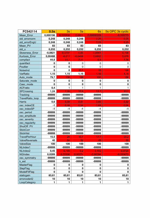
Indices for FC542114

FC542114 0.5s 3s 5s 6s 5s OPC 3s cyclic Mean_Error 0,000196 0,000435 0,0011 0,00000209 -0,000775 std_errornorm 0,248 0,248 0,248 0,25 0,25 std_errorEngU 0,248 0,248 0,248 0,25 0,25 Mean_PV 83 83 83 83 83 std_u 0,232 0,232 0,232 0,232 0,232 Skewness_Error -0,0821 -0,0791 -0,05 -0,0941 -0,108 Kurtosis_Error 0,00488 -0,017 -0,0458 0,0502 0,076 compfact 44,6 11,1 7,41 6,5 7,76 quantfact 0 0 0 0 0 Poutlier 0 0 0 0 0 NoiseInd 0 0 10,1 15 100 VarRatio 1,15 1,15 1,15 1,16 1,16 Auto_mode 79,7 100 100 100 100 Saturate_mode 0 0 0 0 0 Casc_mode 0 0 0 0 0 ACFratio 0,4 1 1 1 1 SPCrossing 1,24 7,35 11,9 13,7 11,7 Tracking -99999 -99999 -99999 -99999 -99999 TravelRatio_loop -99999 -99999 -99999 -99999 -99999 Harris 0,6 0,88 0,81 0,86 0,82 osc_indexCE -1 -0,46 -0,54 -0,68 -0,04 osc_indexSP -1 -1 -1 -1 -1 osc_period -99999 -99999 -99999 -99999 -99999 osc_amplitude -99999 -99999 -99999 -99999 -99999 osc_severity -99999 -99999 -99999 -99999 -99999 osc_regularity -99999 -99999 -99999 -99999 -99999 ShutOff_PV -99999 -99999 -99999 -99999 -99999 StickCorr -99999 -99999 -99999 -99999 -99999 StickHist -99999 -99999 -99999 -99999 -99999 TravelPerHour 15,5 24 19,7 17,7 20,2 ValveReversals 40 64 52 49 55 ValveSize 100 100 100 100 100 NLIndex1 -99999 -99999 -99999 -99999 -99999 NLIndex2 0,45 0,195 0,2 0,102 0,0724 NGIndex 0,0289 0,00386 0,00274 -0,00394 -0,000672 osc_symmetry -99999 -99999 -99999 -99999 -99999 k_est -99999 -99999 -99999 -99999 -99999 MasterFlag 0 0 0 0 0 StepFlag 0 0 0 0 0 ModelFitFlag 0 0 0 0 0 staticgain 83,61 83,61 83,61 83,61 83,61 errorcode42 10 10 10 10 10 LoopCategory 1 1 1 1 1

Indices for FC542119

FC542119 0.5s 3s 5s 6s 5s OPC 3s cyclic Mean_Error -0,00374 -0,00378 -0,00306 -0,00377 0,00671 std_errornorm 0,299 0,299 0,3 0,298 0,207 std_errorEngU 0,299 0,299 0,3 0,298 0,207 Mean_PV 83 83 83 83 83 std_u 2,77 2,77 2,77 2,77 5,58 Skewness_Error 0,0504 0,0371 0,0747 0,0233 0,287 Kurtosis_Error 0,655 0,725 0,793 0,602 5,09 compfact 94,5 16,7 10,9 9,48 14,2 quantfact 0 0 0 0 0 Poutlier 0 0 0 0 0 NoiseInd 0 0 0 0 0 VarRatio 0,0116 0,0116 0,0117 0,0115 0,00138 Auto_mode 75,3 100 100 100 67,9 Saturate_mode 0 0 0 0 0 Casc_mode 0 0 0 0 5 ACFratio 0,02 0,0465 0,0392 0,0465 0,0192 SPCrossing 0,7 4,2 6,9 7,99 1,75 Tracking -99999 -99999 -99999 -99999 -99999 TravelRatio_loop -99999 -99999 -99999 -99999 -99999 Harris 0,36 0,56 0,52 0,56 0,37 osc_indexCE -0,76 -1 -1 -1 -1 osc_indexSP -1 -1 -1 -1 -0,86 osc_period -99999 -99999 -99999 -99999 -99999 osc_amplitude -99999 -99999 -99999 -99999 -99999 osc_severity -99999 -99999 -99999 -99999 -99999 osc_regularity -99999 -99999 -99999 -99999 -99999 ShutOff_PV -99999 -99999 -99999 -99999 -99999 StickCorr -99999 -99999 -99999 -99999 -99999 StickHist -99999 -99999 -99999 -99999 -99999 TravelPerHour 14,1 22 18,6 17,7 21,6 ValveReversals 0 5 5 4 0 ValveSize 100 100 100 100 100 NLIndex1 -99999 -99999 -99999 -99999 -99999 NLIndex2 0,737 0,181 0,147 0,0835 NGIndex 0,07 0,0127 0,00338 -0,00319 osc_symmetry -99999 -99999 -99999 -99999 -99999 k_est -99999 -99999 -99999 -99999 -99999 MasterFlag 0 0 0 0 0 StepFlag 0 0 0 0 0 ModelFitFlag 0 0 0 0 0 staticgain 83,73 83,73 83,73 83,73 83,73 errorcode42 10 10 10 10 10 LoopCategory 1 1 1 1 1

Appendix D

Dead Time Histograms

This appendix includes dead time histograms based on data collected from SodraCell Morrum.

APPENDIX D: DEAD TIME HISTOGRAMS

!

"!

#!

$!

%!

&!!

&"!

& " ' # ( $ ) % * &! +,-.

!"#

$%&'(

)'*((

+,

-%./'01#%'12',%3(2/,

-%./'01#%'41,0(5&.#')(&')*(6'*((+,

!"#$%

&!&"&#&$&%

! ' $ * &" &( &% "& "# ") '! '' '$ '* #" #( #%

+,-.

!"#

$%&'(

)'*((

+,

-%./'01#%'12',%3(2/,

-%./'01#%'41,0(5&.#')(&'*%7%*'*((+,

87

APPENDIX D: DEAD TIME HISTOGRAMS

!

"!

#!

$!

%!

&!!

&"!

& " ' # ( $ ) % * &! +,-.

!"#

$%&'(

)'*((

+,

-%./'01#%'12',%3(2/,

-%./'01#%'41,0(5&.#')(&')*(6'*((+,

!"#$%

&!&"&#&$&%

! ' $ * &" &( &% "& "# ") '! '' '$ '* #" #( #%

+,-.

!"#

$%&'(

)'*((

+,

-%./'01#%'12',%3(2/,

-%./'01#%'41,0(5&.#')(&'*%7%*'*((+,

!"#$%&'

! & "! "& #! #& $! $& %! %& &! && '! '& (! (& )! )& *! *& "!!

+,-.

!"#

$%&'(

)'*((

+,

-%./'01#%'12',%3(2/,

-%./'01#%'41,0(5&.#')(&'3(#+(,101(2'*((+,'

!

&

"!

"&

#!

! " # $ % & ' ( ) * "! +,-.

!"#

$%&'(

)'*((

+,

-%./'01#%'12',%3(2/,

-%./'01#%'41,0(5&.#')(&'+&%,,"&%'*((+,'

!"#$%&'

! & "! "& #! #& $! $& %! %& &! && '! '& (! (& )! )& *! *& "!!

+,-.

!"#

$%&'(

)'*((

+,

-%./'01#%'12',%3(2/,

-%./'01#%'41,0(5&.#')(&'3(#+(,101(2'*((+,'

!

&

"!

"&

#!

! " # $ % & ' ( ) * "! +,-.

!"#

$%&'(

)'*((

+,

-%./'01#%'12',%3(2/,

-%./'01#%'41,0(5&.#')(&'+&%,,"&%'*((+,'

!"#$%

&!&"&#

! ' &! &' "! "' (! (' #! #' '! '' $! $' )! )' %! %' *! *' &!!

+,-.

!"#

$%&'(

)'*((

+,

-%./'01#%'12',%3(2/,

-%./'01#%'41,0(5&.#')(&'0%#+%&.0"&%'*((+,

Appendix E

Result from Index Layer forFC442064

This appendix includes results from performance indices in CLAM (before andafter thresholding).

91

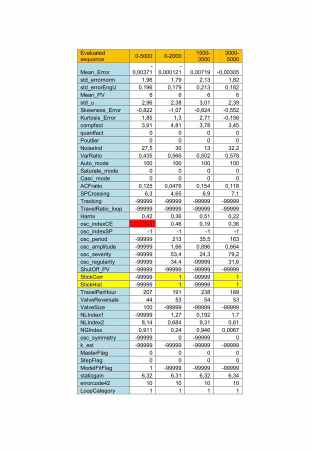
APPENDIX E: RESULT FROM INDEX LAYER FOR FC442064

Table 6: Result from index calculations. Evaluated sequence 0-5000 0-2000 1500-

3500 3000-5000

Mean_Error -

0,00371 -

0,000121 0,00719 -0,00305 std_errornorm 1,96 1,79 2,13 1,82 std_errorEngU 0,196 0,179 0,213 0,182 Mean_PV 6 6 6 6 std_u 2,96 2,38 3,01 2,39 Skewness_Error -0,822 -1,07 -0,824 -0,552 Kurtosis_Error 1,85 1,3 2,71 -0,156 compfact 3,91 4,81 3,78 3,45 quantfact 0 0 0 0 Poutlier 0 0 0 0 NoiseInd 27,5 30 13 32,2 VarRatio 0,435 0,566 0,502 0,578 Auto_mode 100 100 100 100 Saturate_mode 0 0 0 0 Casc_mode 0 0 0 0 ACFratio 0,125 0,0476 0,154 0,118 SPCrossing 6,3 4,65 6,9 7,1 Tracking -99999 -99999 -99999 -99999 TravelRatio_loop -99999 -99999 -99999 -99999 Harris 0,42 0,36 0,51 0,22 osc_indexCE -1 0,46 0,19 0,36 osc_indexSP -1 -1 -1 -1 osc_period -99999 213 35,5 163 osc_amplitude -99999 1,66 0,896 0,664 osc_severity -99999 53,4 24,3 79,2 osc_regularity -99999 34,4 -99999 31,6 ShutOff_PV -99999 -99999 -99999 -99999 StickCorr -99999 1 -99999 1 StickHist -99999 1 -99999 1 TravelPerHour 207 191 238 189 ValveReversals 44 53 54 53 ValveSize 100 -99999 -99999 -99999 NLIndex1 -99999 1,27 0,192 1,7 NLIndex2 8,14 0,684 9,31 0,61 NGIndex 0,911 0,24 0,946 0,0067 osc_symmetry -99999 0 -99999 0 k_est -99999 -99999 -99999 -99999 MasterFlag 0 0 0 0 StepFlag 0 0 0 0 ModelFitFlag 1 -99999 -99999 -99999 staticgain 6,32 6,31 6,32 6,34 errorcode42 10 10 10 10 LoopCategory 1 1 1 1

Table 7: Result from index layer after thresholding. Evaluated sequence

0-5000

0-2000

1500-3500

3000-5000

Mean_Error std_errornorm X X X X std_errorEngU Mean_PV std_u Skewness_Error Kurtosis_Error compfact X X X X quantfact Poutlier NoiseInd VarRatio Auto_mode X X X X Saturate_mode Casc_mode ACFratio X X X X SPCrossing X Tracking TravelRatio_loop Harris X X X X osc_indexCE X X X osc_indexSP osc_period osc_amplitude osc_severity X X osc_regularity ShutOff_PV StickCorr X X StickHist X X TravelPerHour ValveReversals ValveSize NLIndex1 X NLIndex2 X X X X NGIndex X X X osc_symmetry k_est MasterFlag StepFlag ModelFitFlag staticgain errorcode42 LoopCategory

UpphovsrattDetta dokument halls tillgangligt pa Internet — eller dess framtida ersattare —under 25 ar fran publiceringsdatum under forutsattning att inga extraordinaraomstandigheter uppstar.

Tillgang till dokumentet innebar tillstand for var och en att lasa, ladda ner, skri-va ut enstaka kopior for enskilt bruk och att anvanda det oforandrat for ickekom-mersiell forskning och for undervisning. Overforing av upphovsratten vid en senaretidpunkt kan inte upphava detta tillstand. All annan anvandning av dokumentetkraver upphovsmannens medgivande. For att garantera aktheten, sakerheten ochtillgangligheten finns det lasningar av teknisk och administrativ art.

Upphovsmannens ideella ratt innefattar ratt att bli namnd som upphovsmani den omfattning som god sed kraver vid anvandning av dokumentet pa ovan be-skrivna satt samt skydd mot att dokumentet andras eller presenteras i sadan formeller i sadant sammanhang som ar krankande for upphovsmannens litterara ellerkonstnarliga anseende eller egenart.

For ytterligare information om Linkoping University Electronic Press se forlagetshemsida http://www.ep.liu.se/

CopyrightThe publishers will keep this document online on the Internet — or its possi-ble replacement — for a period of 25 years from the date of publication barringexceptional circumstances.

The online availability of the document implies a permanent permission foranyone to read, to download, to print out single copies for his/her own use andto use it unchanged for any non-commercial research and educational purpose.Subsequent transfers of copyright cannot revoke this permission. All other uses ofthe document are conditional on the consent of the copyright owner. The publisherhas taken technical and administrative measures to assure authenticity, securityand accessibility.

According to intellectual property law the author has the right to be mentionedwhen his/her work is accessed as described above and to be protected againstinfringement.

For additional information about the Linkping University Electronic Press andits procedures for publication and for assurance of document integrity, please referto its www home page: http://www.ep.liu.se/

c� Calle Skillsater

Evaluation and Conﬁguration of a Control Loop Asset...

Documents

Transcript of Evaluation and Conﬁguration of a Control Loop Asset...