Evaluating the Health of Wetlands - British Columbia
61
FOREST AND RANGE EVALUATION PROGRAM Protocol for Evaluating the Health of Wetlands (Wetland Management Routine Effectiveness Evaluation) Version 2.1 January 2021
Transcript of Evaluating the Health of Wetlands - British Columbia

FOREST AND RANGE EVALUATION PROGRAM
Protocol for
Evaluating the Health of Wetlands
(Wetland Management Routine Effectiveness Evaluation)
Version 2.1
January 2021

Wetland Management Routine Effectiveness Evaluation – January 2021
2
Citation: Fletcher, N.F., Tripp, D.B., Hansen, P.L., Nordin, L.J., Porter, M., and Morgan, D. 2021. Protocol for the Wetland Health Management Routine Effectiveness Evaluation. Forest and Range Evaluation Program, B.C. Ministry of Forests, Lands, Natural Resources Operations and Rural Development, Victoria, B.C. Prepared by: Neil Fletcher, BC Wildlife Federation Derek Tripp, Tripp & Associates Consulting Ltd. Paul Hansen, Ecological Solutions Group LLC Lisa Nordin, B.C. Ministry of Forests, Lands, Natural Resources Operations and Rural Development Marc Porter, ESSA Technologies Don Morgan, B.C. Ministry of Environment & Climate Change Strategy Maureen Nadeau, BC Wildlife Federation Jason Jobin, BC Wildlife Federation Tobias Roehr, BC Wildlife Federation Additional Input Provided by: Suzanne Bailey, University of Alberta Nora Billy, St’at’imc Government Services Wade Brunham, ERM Darwyn John, St’at’imc Government Services Alicia Krupek, Splitrock Environmental Karen Kubiski, Carrier Chilcotin Tribal Council Natasha Lukey, Okanagan Nation Alliance Kim North, Splitrock Environmental Daryn Scotchman, Splitrock Environmental Crystal Wallace, Lower Nicola Indian Band Special thanks to members of the Steering Technical Committee of the Skeena Environmental Sustainability Initiative for offering additional input into an earlier version of this protocol. For more information on BC Forest and Range Evaluation Program (FREP) publications, visit our web site at:http://www2.gov.bc.ca/gov/content/industry/forestry/managing-ourforest-resources/integrated-resource-monitoring/forest-range-evaluation-program/frepreports-extension-notes. © 2021 Province of British Columbia When using information from this or any other FREP publication, please cite fully and correctly.

Wetland Management Routine Effectiveness Evaluation – January 2021
3
Table of Contents
Introduction .................................................................................................................................................. 6
Recommended Steps for a Wetland Health Evaluation ......................................................................... 11
Recording Data ........................................................................................................................................ 22
Health Scoring Questions ........................................................................................................................ 23
Vegetation ........................................................................................................................................... 23
1.Vegetative cover .......................................................................................................................... 23
2. Invasive and/or noxious spp ....................................................................................................... 23
2.a) Invasive and/or Noxious Plant Canopy Cover ........................................................................ 23
2.b) Invasive and/or Noxious Plants distribution .......................................................................... 24
3. Coverage of disturbance-caused undesirable species ................................................................ 24
4. Vegetation compared to a healthy unmanaged wetland and riparian plant communities ....... 25
4.a) Wetland plant community structure ..................................................................................... 25
4.b) Wetland plant recruitment, form and vigor in the wetland .................................................. 26
4.c) Upland plant community structure ........................................................................................ 27
4.d) Uplands plant recruitment, form and vigor ........................................................................... 27
4.e) Long-term trajectory of the vegetation community .............................................................. 28
5. Sufficient vegetation to minimize windthrow, maintain adequate screening, visual cover and
LWD supply ..................................................................................................................................... 29
5.a) Retention of non-merchantable conifer, understory deciduous trees, shrubs and herbaceous
vegetation within 20m of the wetland edge................................................................................... 27
5.b) Retention in the CDF, PP, BG, CWHxm, dm, ds and IDFxh, xw, and xm BEC units ................ 29
5.c) Retention in the ESSF, MS, ICH, MH, CWHvm, mm, ms, ws and IDFdm, dk1, and dk2 units 30
5.d) Retention in the SWB, SBS, SBPS, BWBS, CWHvh and IDFww, mw, dk3, and dk4 units ....... 30
5.e) Percent live woody vegetation removed from wetland, other than browsing. .................... 29
6. Heavy browsing and grazing ....................................................................................................... 28
6.a) Heavy browsing ...................................................................................................................... 28
6.b) Heavy grazing ......................................................................................................................... 29
6.c) Seedlings or saplings of palatable tree and shrub species ..................................................... 29
Soils ..................................................................................................................................................... 32
7. Bare and compacted ground ....................................................................................................... 32
7.a) Bare and compacted ground .................................................................................................. 33

Wetland Management Routine Effectiveness Evaluation – January 2021
4
7 b)Bare soil within and/or hydrologically connected ................................................................. 33
Morphology ......................................................................................................................................... 34
8. Physically altered site .................................................................................................................. 34
8.a) Proportion of altered topography .......................................................................................... 34
8.b) Severity of the physical alteration ......................................................................................... 35
9.Intact wetland woody debris processes ...................................................................................... 35
9.a) Standing dead trees (snags) and decadent trees (dying trees) density ................................. 36
9.b) Standing dead tree diversity .................................................................................................. 37
9.c) Stable coarse woody debris.................................................................................................... 38
9.d) Diversity of coarse woody debris ........................................................................................... 38
10. Windfirm buffer ........................................................................................................................ 39
10.a) Riparian windthrow in RMA without an RRZ or designated WTP ...................................... 37
10.b) Riparian windthrow in RRZ or WTP ...................................................................................... 40
10.c) Wildlife Trees ........................................................................................................................ 38
Hydrology ............................................................................................................................................ 38
11. Changes in the hydrologic regime ............................................................................................. 38
11.a) Severity of hydrologic changes ............................................................................................ 38
11.b) Dead trees or shrubs at the wetland edge? ......................................................................... 39
11.c) Younger age class plants or trees encroachment ................................................................ 39
11.d) Stream channel incisement.................................................................................................. 39
11.e) Natural surface or subsurface wetted areas. ....................................................................... 43
12. Threats to water levels in the wetland ..................................................................................... 43
12.a) Outlet structure . .................................................................................................................. 43
12.b) Active headcuts below or within the wetland ..................................................................... 43
12.c) Disturbed shoreline of the wetland ..................................................................................... 43
12.d) Deep binding rootmass ........................................................................................................ 44
Water Quality ...................................................................................................................................... 44
13. Water quality of the wetland ................................................................................................... 45
13.a) Excessive nutrient loading .................................................................................................... 45
13.b) Basic water quality parameters ........................................................................................... 45
Landscape ........................................................................................................................................... 46
14. Surrounding habitat .................................................................................................................. 46
14.a) Total riparian area disturbance ............................................................................................ 46

Wetland Management Routine Effectiveness Evaluation – January 2021
5
14.b) Visible shoreline ................................................................................................................... 47
14.c) Right-of-ways within 100 m ................................................................................................. 47
14.d) Percent mature and old forest within two kilometers …………………………….…….………………..45
15. Surface and subsurface flows to the wetland intact................................................................. 49
15.a) Mapped and unmapped streams diversion ......................................................................... 49
15.b) Contributing basin intercepted by roads or ROWs .............................................................. 47
Appendix 1 – Recommended Field Sampling Sequence ....................................................................... 51
Appendix 2 - Common invasive and noxious plants within BC ………………………………………………………….. 53
Appendix 3 – Select list of Culturally Significant Plants to Indigenous Communities in BC ................... 56
Appendix 4 – Wetland Indicator Status Categories ................................................................................ 60
Appendix 5 - Minimal Targets for Mature and Old Forest Coverage ...................................................... 61
List of Figures
Figure 1. A key to the different freshwater wetland ecological classes .......................................................9
Figure 2. Wetland boundaries for health assessment ..................................................................................10
Figure 3. Key to wetland riparian classification ............................................................................................13
Figure 4. Placement of transects and plots, and associated calculations.....................................................16
Figure 5. Distribution Codes for invasive species .........................................................................................24
Figure 6. Visual appearance codes for wildlife trees ....................................................................................37
Figure 7. Edatopic grid for abiotic factors and their relationship with different aquatic classes .................46
Figure 8. Map of Right of Ways within 500m buffer to identify potential vantage points ...........................47
Figure 9. Example of Road impinging within 100m of wetland area ............................................................48
Figure 10. Example Spatial query within a 2 km buffer of the wetland .......................................................49
Figure 11. Contributing Basin Assessments ..................................................................................................47
List of Tables Table 1. Riparian management distances .....................................................................................................13
Table 2. Description of Dominant Upland vegetation Strata Around Perimeter of Wetland…………………….16
Table 3. Transect Information………………………………………………………………………………………………………………….19 Table 4. Organic Soils Classification Table based on the Von Post Scale ......................................................22
Table 5. Example of a completed vegetation plot table ...............................................................................23
Table 6. List of Common disturbance-increaser species in BC .....................................................................26
Table 7 Structures and Vegetation Form, Vigor, and Recruitment within wetland ....................................28
Table 8. Structures and Vegetation Form, Vigor, and Recruitment upland .................................................28
Table 9. Snags and Coarse Woody Debris Indicators ....................................................................................37
Table 10. Tree Diameter Classes ...................................................................................................................38
Table 11. Decay Classes for Coarse Woody Debris .......................................................................................39

Wetland Management Routine Effectiveness Evaluation – January 2021
6
Introduction
This guidance document provides supplementary details to the BC Ministry of Forests, Lands, Natural Resource Operations and Rural Development (FLNRORD) field form for evaluating the health of wetlands. Field technicians are expected to read this protocol prior to using the wetland health evaluation form in the field. This document provides information on site selection, sampling protocol, and interpretation of the questions in the form. Technicians are encouraged to refer to this document when evaluating their first few wetlands of the year. Reviewing the document on a regular basis will help calibrate interpretation skills. The Resource Planning and Assessment Branch within the Ministry of Forests, Lands, Natural Resource Operations and Rural Development (FLNRORD) and the Ecosystems Branch in the Ministry of Environment and Climate Change Strategy (ENV) developed this Wetland Health Assessment Form and Protocol to complement their current suite of monitoring tools within the Forest and Range Evaluation Program (FREP). One example of a well-established FREP tool is the Riparian Management Routine Effectiveness Evaluation Field Form with the associated Protocol, which assesses stream/riparian condition. The objective of this FREP Wetland Health Assessment Form and Protocol is to allow for persons with basic working knowledge of wetlands to evaluate the health of wetlands within or in proximity to industrial development activities (e.g., forestry). Field evaluators may be forest and range practitioners, First Nation’s stewardship members, consultants, land managers, or other land users. This Wetland Protocol is a coarse-level filter for assessing the health of wetlands. The assessment form is intended to be completed mainly in the field, promote consistency among users, gather pertinent data to inform the health of the wetland, and be cost effective as a tier 2 approach for monitoring (i.e., relatively quick to use in the field (1-4 hours). One of the advantages of the protocol is that it is a relatively low-cost method to assess wetlands in the field and can enable comparative analysis among numerous sites. A wetland flagged with poor health may require further inspection, or a more detailed analysis may be required to investigate a wetland more thoroughly or to meet other objectives of land managers. A healthy wetland is a measure of its capacity to perform a number of functions in the environment. Society assigns value to many wetland functions as they can support both healthy landscapes and healthy communities. Although not all wetlands perform the same functions, some of the functions include: sediment trapping, shoreline maintenance, wave energy dissipation, water storage, aquifer or stream recharge, maintenance of biotic diversity, carbon cycling and storage, nutrient cycling and absorption, and primary productivity. The values we derive from these functions may include: flood control, clean water, and provision of food and medicinal products. In order for a wetland to perform these functions effectively, it requires healthy vegetation, intact soils, specific hydrologic regimes, and an appropriate connectivity to the broader landscape. This protocol helps categorize the health of a wetland as: properly functioning; functioning, but at risk; functioning, but at high risk; or not properly functioning. There are many wetland evaluation protocols in North America that quantify a wetland’s functioning condition or assess its health, but none that have been formally and broadly adopted by the Province of BC. This protocol represents the first to be developed at a provincial scale for measuring wetland health. For clarity, the protocol does not quantify specific measurable processes of a wetland (e.g., the amount of

Wetland Management Routine Effectiveness Evaluation – January 2021
7
flood retention of a particular wetland), which requires a separate inventory framework. Instead, it focuses on observed or potential impacts that would affect a wetland’s ability to perform functions. The development of this protocol is adapted from several existing protocols. Contributing or supporting literature includes:
• Riparian Area Management: A User Guide to Assessing Proper Functioning Condition and Supporting Science for Lentic Areas. TR 1737-16 1999 Revised 2003. USDA and Bureau of Land Management.
o This guide provides a solid foundation for assessing wetland health and recommends a variety of tools and approaches. The lead author, Don Pritchard, helped establish and popularize the concept of Proper Functioning Condition. However, the indicators within the document rely on a team of experts reaching consensus in order to determine the health of the site. Many of the indicators recommended in this document made their way into the FREP riparian protocol, but additional thresholds and associated guidance were developed to ensure consistency among users.
• Riparian Management Effectiveness Evaluation Field Form and Protocol. 2017. B.C. Ministry of Forests, Lands, Natural Resource Operations and Rural Development.
o This protocol, developed by the Forest and Range Evaluation Program (FREP), was closely reviewed for elements to transfer. It is expected that field crews completing the riparian protocol will also complete the wetlands protocol. The format for the FREP wetlands form is similar to the riparian version for ease of use and to promote consistency. Several of the indicators that relate to riparian areas are the same or slightly modified for the wetlands protocol.
• Alberta Lentic Wetland Health Assessment Survey; and Alberta Lotic Wetland Health Assessment Survey for Streams and Small Rivers. 2014. Alberta Riparian Habitat Management Society.
o These two protocols, managed in Alberta by the Alberta Riparian Habitat Management Society, were developed by Paul Hansen and other experts working with the Ecological Solutions Group LLC. Modified versions of the protocol have been applied in Saskatchewan and numerous US states by land managers, as well as by Canadian and US federal agencies. The indicators and protocols have been refined over 20 years, where thresholds and weighting of indicators were developed by a group of experts using the Delphi method. In lieu of a BC wetland health assessment standard, these protocols have been used ad-hoc at a regional scale in BC by FLNRORD, BC Parks, the Nature Conservancy of Canada, and several consultants. Most of the applications have been on range land in the interior; however, according to the lead author, Paul Hansen, the forms were designed to be used for broad application and have been tested on the BC coast with satisfactory transferability. In several cases, where the thresholds for indicators in the FREP form did not exist, a threshold for a Yes or No was derived from the Alberta protocols. At the time of the development of this current FREP protocol, three separate initiatives in BC were attempting to integrate the Alberta Lentic and Lotic protocols into a BC framework. A key difference is that questions in the FREP version also consider natural disturbances, as opposed to only human-caused impacts, so data on the natural variability of wetland health may be determined. With permission from Paul Hansen, several of the guidance question indicators were replicated, and modified as needed, from these two Alberta protocols.

Wetland Management Routine Effectiveness Evaluation – January 2021
8
Wetland Delineation The delineation of the wetland polygon is a critical step in the FREP Wetland Health Assessment as many of the indicator questions are heavily influenced by the defined polygon unit. For example, the percent cover of invasive species will change dramatically with substantial changes in the assessment area. The boundaries can be determined pre-field and adjusted in the field. A copy of recent high-resolution aerial imagery with an overlay of the boundary will improve the assessment in the field. The evaluator may choose the measuring tool on Google Earth imagery, ArcMap, FREPmap (for government staff) or QGIS to draw a polygon boundary and calculate the area. To get started, provincial wetland layers are available from the BC Data Catalogue, such as wetlands in the Freshwater Atlas and in the Vegetation Resource Inventory. As a word of caution, these wetland boundaries may poorly resemble what is found on the ground, as they are generally created from remote imagery. If available, wetlands may be better delineated on imagery or the forest site plan for a cutblock, and the boundaries refined after field verification. FLNRORD stewardship officers may also be able to calculate wetland areas using the online FREPmap tool that includes recent SPOT imagery. On-the-fly calculations are possible with mobile map apps, such as Avenza. In the near future, drones may serve as a very helpful tool to gather real time data (i.e., both wetland delineation and determining values for some of the indicators). Ensure to save screenshots of any variances in wetland boundaries, that you can then include in your data submission. In some cases, the evaluator may find that the boundaries need to shift once they get out to the field. The natural boundaries between an upland area and a wetland can generally be determined by a distinct change in vegetation of water-dependent (obligate) or water-tolerant (facultative) species to more terrestrial plant species. The presence of hydric soils (i.e., gleying or mottling of mineral soils within the first 30 cm, the presence of poorly decomposed organic soils (e.g., peat), or a near surface water table can also help delineate the terrestrial/wetland boundary. At the interface of the wetland and deeper water, such as a lake, the wetland is delineated as the vegetated zone with greater than 10% rooted vegetation and less than 2m depth in mid-summer. Any modifications of the boundaries in the field should be included with the assessment. In some cases, where heavy disturbance has occurred, the boundaries of the wetland may not match the natural observable boundaries. The evaluation relies on understanding the potential area of wetland prior to any disturbances. If there has been soil deposited into the wetland or a decline in water level (and thus a retraction of the wetland area), the evaluator will need to consider the historical context of where the wetland would have been prior to the disturbance to evaluate the impacts. This is one of the more challenging parts of the protocol to consider, especially in heavily modified areas. Old aerial imagery, traditional or community knowledge, or onsite evidence of disturbance may help to determine the historic extent of the wetland. The evaluator will need to take detailed notes and provide a rationale for any changes in the boundary of the assessment area. The evaluator may choose to only complete an assessment of a portion of a wetland. One reason to do so may be to subsample a wetland that is too large to feasibly assess. Again, the evaluator will need to provide details and document their rationale for modifying the boundary. The interpretation of the various ecological classes and plant associations within the wetland will help the evaluator answer some of the questions (e.g., Question 4. “Is the vegetation of the entire polygon generally characteristic of what the healthy unmanaged wetland and riparian plant communities are

Wetland Management Routine Effectiveness Evaluation – January 2021
9
normally?”). Field crews should become familiar with using the book, Wetlands of British Columbia: a guide to identification (2004), which provides substantial detail of many of BC’s most common wetland plant associations and often indicates typical progressions between plant associations of wetter and drier sites. However, the book does not contain all wetlands and the assessor will encounter sites that do not conform to the descriptions. Some wetlands may be in transition between two plant associations, while others are not documented. More recent field guides to ecosystem classification may provide additional detail to plant associations in specific regions. At a minimum, the field evaluator should become familiar with the various freshwater ecosystem classes: bogs, fens, marshes, swamps, and shallow water. Figure 1 provides a key to the different wetland ecological classes. Patterns of vegetation can often be observed from remote imagery, and differences in patterns often indicate a change between plant associations or wetland ecological classes. For the purposes of this assessment, the evaluator may not need to break the wetland into the various classes, but knowledge of the various types within it can aid in interpretation. See Figure 2 for examples of established wetland boundaries.
Figure 1. A key to the different freshwater wetland ecological classes (Source: Mackenzie 2012.
Biogeoclimatic ecosystem classification of non-forested ecosystems in British Columbia. B.C. Min. For.,
Res. Br., Victoria, B.C. Tech. Rep. 068.). The “surface tier” mentioned in the chart is 40 cm thick excluding
any loose litter, crowns of sedges and reeds, or living mosses. Shallow organic soils over mineral soil or

Wetland Management Routine Effectiveness Evaluation – January 2021
10
bedrock may have only a surface tier. Of note: in rare cases, some swamps may also contain mesic soils
(e.g., Ws05).
Figure 2. Examples of Wetland boundaries established for the health assessment with wetland ecological
classes identified. For the purposes of this assessment, in most cases, the boundaries should be
established to the extent they would be pre-disturbance. In the example shown at the top of this figure, a
road was constructed over a portion of the wetland, and the original extent of the wetland was estimated
on the northeast section of the wetland.

Wetland Management Routine Effectiveness Evaluation – January 2021
11
Recommended Steps for a Wetland Health Evaluation
The following guidance is provided to help complete the first few sections of the field form. Review the
recommended field sampling sequence in Appendix 1 for an efficient order of progressing through tables
and checklists once in the field.
STEP 1 – OFFICE REVIEW AND PREPARATION:
Conduct an office review of the wetland polygon area before going out into the field. Complete the
information in Tables 1 to 3 (T.1-T.3) of the field form to the best of your ability. Many of the questions in
this section can be completed in the office but may need to be revised once you arrive in the field.
Useful GIS layers include topographic information (to delineate the contributing basin of the wetland),
stream layers, tenure boundaries (range, aggregate, recreation, utilities, etc.), biogeoclimatic information,
forest age classes (i.e., from the Vegetation Resource Inventory), cutblocks, and right-of-ways (e.g., roads,
pipelines, etc.). Good quality remote imagery will also be useful to complete some sections, such as
identifying any mass wasting that may have occurred.
Contact the licensee of the cutblock associated with the wetland to inform them of the intention of
entering their operating area, invite them to attend, and request their site plan and any other related
information to help with the assessment. The licensee may be able to also inform you of any gates or
decommissioned roads that would be important for planning your site visit. It is important to read over
the forestry site plan for the wetland of interest, as well as the land use plan if possible. This will ensure a
general overview of what management strategies were prioritized and how the wildlife/land was
considered.
Wetland Information (T.1.1)
Wetland ID – A unique identifier for the wetland (found by querying the spatial information).
Source of wetland polygon – Select or describe the source that best reflects the most accurate
boundaries of the wetland (you may need to confirm this once in the field). Sources may include
the Freshwater Atlas (FWA), site plans, the Vegetation Resource Inventory, digitized layers
defined by the user, etc.
Biogeoclimatic Ecosystem Classification (BEC) – record the BEC for the area.
Natural Disturbance Type (NDT) – record the natural disturbance type (e.g., NDT1). This will be
needed to help answer Q14, and can be found by cross-referencing the BEC sub-zone and variant
in the Biodiversity Guidebook. (https://www.for.gov.bc.ca/hfd/library/documents/bib19715.pdf )
If unknown, both BEC and NDT can be found by following these 5 steps: 1. Launch iMap BC: https://maps.gov.bc.ca/ess/hm/imap4m/ 2. Zoom to wetland location of interest.
Note: If you are unsure where your wetland is, open up the wetlands layer within the Freshwater Atlas which “may” include the wetland of interest or at least help better orient yourself. Do this by clicking under tab “Data Sources”, select “Add Provincial Layers”. In the pop-up “Add/Remove Map Information”, click to expand options under “Base Maps”, then click to expand options within “Freshwater Atlas”, then select “FWA – Wetlands – Colour Theme” and press OK
Wetland Management Routine Effectiveness Evaluation – January 2021
12
3. Select tab “Data Sources” and select “Add Provincial Layers” 4. In the pop-up “Add/Remove Map Information”, click to expand options under “Forest
Grasslands and Wetlands”, then click to expand options within “BEC Analysis – Zones/Subzones/Variants – All”, then select “BEC Analysis – Zones/Subzones/Variants – Coloured Themes” and press OK
5. Under the “Find Tab”, select the icon labeled “Point” (it has an icon of a cross-hairs with a blue circle with the letter “i”), then hover your cursor over the wetland of interest, and then left click. A side bar will appear labeled Identify Results. Select the “BEC Analysis – Zones/Subzones/Variants – Colour Theme”. The BGC for the area you selected will appear (e.g., Interior Douglas Fir), click on the symbol “>”, next to the listed BGC, and details for the BGC will appear. Record both the BGC Label including the variant (e.g., IDFxh1), and the Natural Distrubance Type (e.g.,NDT4). Put these in the appropriate fields of the form.
Total Wetland Size – Record in square meters (note: 1 ha = 10,000 m2)
Hydrogeomorphic System – Select from estuarine, fluvial, basins & hollows, seepage slopes, lacustrine, ponds & potholes, and marine. Refer to Mackenzie and Moran 2004, (p41) for a descriptor of each type.
Wetland is hydrologically connected to a stream? – Record yes or no. Helpful tip: Calculate wetland size information on page 3 of the field form. The field evaluator must document Wetland Size, Total Polygon Assessed, and Total Upland Area (10 m buffer) (See pg 16 of the protocol for further information). These values represent the actual wetland size and assessed area as the field evaluator may be required to make adjustments once they visit the site and determine the true boundaries and any access issue. It is helpful, however, to measure these values using desktop tools prior to going into the field, and then adjust if modifications are necessary. This will allow the field evaluator to make many of the subsequent calculations in the field that require these values. First Nations Information (T.1.2)
List all First Nations territory in which the wetland is located and contact the chief(s) or band offices (as
appropriate). The Province of BC’s Consultative Area Database can help you determine which First
Nations may have an interest in a particular wetland. Explain the objective of conducting a wetland
health assessment and invite interested individuals to participate in the field-based component.
Opening Information (T.1.3) Complete this section if the wetland is within 2 riparian management area (RMA) widths of a cutblock.
District – The official three-letter code for the natural resource district (e.g., DCR for Campbell
River Natural Resource District).
Opening ID – The unique 5-7 digit code from RESULTS (used each year in the random selection of
cutblocks for sampling).
Licensee – The company that holds the forest license for the block.
Forest License – The forest license recorded for the cutblock in RESULTS.

Wetland Management Routine Effectiveness Evaluation – January 2021
13
Block – The designation used by the licensee on their logging plan or site plan map.
Harvest Year – The year timber in the selected block was harvested along the sample reach.
Harvest Location – The location of harvesting in the block relative to the sample wetland; record
north, east, south, and/or west, as applicable.
Wetland Riparian Class on Plans – Record the wetland riparian class (W1-W5 or unclassified
wetland) indicated on the logging plan and/or site plan map.
Wetland Riparian Class in Field – In most cases, this is the same as the wetland riparian class on
the logging plan. Record a different wetland riparian class only if it was misclassified. Wetland
riparian classes are defined in Figure 3. Note: A wetland complex (W5) must consist of two or
more individual wetlands with overlapping riparian management areas and a combined wetland
area of 5 ha or more.
Record the riparian management area (RMA), riparian reserve zone (RRZ), and riparian
management zone (RMZ) in metres (see Table 1).
Figure 3. Key to wetland riparian classification (Source: Forest Practices Code Guidebook: Riparian
Management Area Guidebook 1995).
Wetland Riparian Class RMA (m) RRZ (m) RMZ (m)
NCW 0 0 0
W1 50 10 40
W2 30 10 20
W3 30 0 30
W4 30 0 30
W5 50 10 40
Table 1. Associated riparian management distances from edge of wetland based on wetland riparian class from the B.C. Riparian Management Area Guidebook. Note: NCW = non-classified wetland.

Wetland Management Routine Effectiveness Evaluation – January 2021
14
Riparian/Buffer Retention Information (T.1.4)
Riparian/Buffer Retention – Record the following attributes related to the wetland buffer. The buffer can
have 3 potential treatments: full retention, partial retention, or no retention. If you feel the information
on riparian retention in T.1.4 does not adequately describe the condition of the riparian area, please add
a sketch of the riparian area on page 16 of the field form. A photograph or two of the riparian area can
also be invaluable in describing the riparian conditions.
Length of wetland perimeter within assessment polygon (m): Record in meters the length around
the wetland edge.
Length along wetland perimeter with full treed retention (m): Record in meters the length of the
perimeter where the riparian area has had no harvesting.
Average width of full treed retention present (from wetland edge) (max 100m): Record the width
of full retention or record 100 m if the width is greater than 100 m.
Length along wetland perimeter with partial retention (m): Record in meters the length of the
perimeter where the riparian area has had recent partial/selective harvesting.
Average width of treed retention present with partial retention (from wetland edge - max 100 m):
Record the width of partial retention or record 100 m if the average width is greater than 100 m.
Average treed retention present with partial retention (% of basal area): Record % of basal area
remaining.
Length along wetland perimeter with no retention (m): Record in meters the length of the
perimeter where clearcut harvesting is adjacent to the wetland boundary.
Description of dominant upland vegetation strata around perimeter of wetland (T.1.5)
Table T.1.5 of the field form is used to stratify abutting upland areas in order to place sampling transects
and to describe the associated upland characteristics. The evaluator will want to stratify the perimeter to
represent major differences in the land-base abutting the wetland that may positively or negatively
influence the functioning condition of the wetland.
Upland Descriptor for Vegetation Strata and Age – Provide a descriptor for dominant vegetation
types within 100 m perpendicular to the wetland perimeter. For example, if the first 30 m of the
upland area from the wetland edge is treed retention and the next 70 m is recent cutblock, record
recent cutblock. Descriptors may include: recent cutblock; young/mature/old coniferous;
young/mature/old deciduous; young/mature/old mixed forest; lake/pond abutting; stream/river
abutting; grassland, other.
Disturbance: Record disturbance type. For example, if the upland descriptor was “young forest” ,
it may be because it was burned. If that is the case, record “recent fire” for disturbance type.
Descriptors may include: recent cutblock, old cutblock, recent fire, insect infestation, log sort –
landing, road within 100 m, other.

Wetland Management Routine Effectiveness Evaluation – January 2021
15
Width – Record the approximate distance the dominant vegetation type extends beyond the
wetland perimeter. If it extends beyond 100 m, then record 100 m.
Length Along Wetland Perimeter – Record the length of the wetland perimeter occupied by the
dominant vegetation type.
Fraction along wetland perimeter- This is the fraction that is composed of your upland type. If
your total perimeter is 800m and the cutblock is along 200m, the fraction is 0.25 (or 25%).
Number of Transects – Record the number of transects to be documented within the wetland for
each strata. For wetlands <5 ha, place up to three transects. If the dominant vegetation type is
homogenous around the wetland edge (e.g., a cutblock surrounds the entire perimeter), then you
may choose to select only two transects. For wetlands with two dominant vegetation types both
with >45% of the perimeter occupied, place two transects in the wetland – one in each type. For
wetlands with two dominant vegetation types, but one type occupies less than 45% of the
wetland perimeter, then place two transects in the dominant upland type and one in the less
dominant. For wetlands with greater than three dominant vegetation types, place a transect in
each vegetation type that occupies >10% of the perimeter.
Location of Transect Along Perimeter Section – To place transects within the stratified vegetation
types, use a random number generator that will mark the location of the transect along the
wetland perimeter. The FREP Wetland Filemaker App will automatically do this for you.
Otherwise, if the cutblock portion occupies 204 metres of the wetland perimeter, then select a
random number between 0 and 204. Using this example, a random number can be generated
very quickly in Microsoft Excel by typing in a cell “=randbetween(0,204)”, which will randomly
generate a number between the two numbers specified. For consistency, set smaller numbers to
larger numbers in a clockwise direction around the wetland perimeter.
Upland Descriptor for Vegetation Strata and Age
Disturbances (s) (e.g., insects, road, cutblock)
Width (m)
Length along perimeter (m)
Fraction along wetland perimeter
Number of Transects
Location(s) of transects along perimeter section
Mature Coniferous Forest
Road 100 370 0.54 1 345 x x
Cutblock Recent Cutblock 80 212 0.31 1 198 x x
Young Mixed Forest
Old Cutblock 100 105 0.15 1 32 x x
Table 2. Example of T.1.5: Description of Dominant Upland vegetation Strata Around Perimeter of Wetland.
Other Developments (T.1.6)
Describe the contributing basin upstream of the wetland and estimate the percent that has been
developed. You can use the tools provided in ArcGIS, QGIS, Google Earth, FREPmap (government only), or

Wetland Management Routine Effectiveness Evaluation – January 2021
16
a georeferenced pdf to draw polygons and calculate the areas of both the watershed and the
development to help estimate this value. Include road right-of-ways, agriculture pastures, existing
cutblocks, transmission lines, and any other man-made features when calculating the area of
development.
Number of Road Crossings – Three numbers are asked for: the number of road crossings within
the polygon being assessed (including the 10m upland area), the number of road crossings in the
wetland, and the number of crossings on any upstream tributaries that flow into the wetland.
Percent of Watershed Developed Upstream – Delineate the watershed area above the wetland
polygon being assessed using topographic map layers and/or imagery and estimate the total
percent area developed to date.
Main Development – Record the main human activity present in the watershed area above the
sample polygon (e.g., roads, forestry (except roads), agriculture, recreation, mining, oil and gas,
transportation, utilities, other, none).
Landscape Indicators (T.2)
Prior to heading out to the field, several of the health indicator questions can be estimated in the office.
Refer to the landscape section starting on page 44 in this document for completing section T.2. on the
form.
Supplementary Management Observations (T.3)
Section T.3 in the form contains supplemental management observations that can be observed either in
the office and/or while on site.
Do the boundaries on the site plan for the wetland coincide with observations in the field?–
Record Y or N.
Was there retention around other wetlands observed on the block? Record Y or N – this may be
best observed from a combination of map and field observation.
Is four-wheel drive access blocked on roads within 100 m from the wetland edge? Record Y or N.
If rangeland is present, were measures taken to reduce/block livestock access to the wetland
edge? Record Y or N. For example, are there any recent fences or logs that appear to purposefully
block or control access to the wetland?
STEP 2 – FIELD BASED OBSERVATIONS
Field surveyors are strongly encouraged print, or take an electronic copy, of the 2-page instructions in
Appendix 1 to take into the field for an efficient step-by-step process to gather field-based
observations.
Once in the field, before starting any measurements, first confirm the wetland is a wetland, the wetland polygon boundary is accurate/appropriate, and the wetland is within two riparian management areas. At the top of the FIELD SAMPLING INFORMATION page (pg 3):

Wetland Management Routine Effectiveness Evaluation – January 2021
17
Check the box for whether sampling is representative of the entire wetland or a portion of the wetland. If only a partial area of a wetland was selected, provide a description on page 18 as to where the wetland polygon was segmented, and provide a rationale for why the partial wetland was selected (e.g., large size, change in management regimes, access blocked, etc.). The entire wetland may not be feasible to assess due to access barriers (e.g., extremely dense brush, deep channels, other safety concerns). After reviewing the site from the office or the field, the evaluator may determine that the wetland poses access barriers and adjust the total polygon assessed. Total Polygon Assessed – Record in m2. For the purposes of this evaluation, the Wetland Polygon
Assessed includes the 10 m spatial buffer for some questions. This measurement is the wetland assessed
size plus the 10 m upland size. This can be calculated using QGIS or FREPmap (for government employees)
by drawing a wetland polygon, then creating a 10m buffer and drawing a polygon around the outer
boundary and calculating total area using the GIS tools.
10 m Upland Size – Record in m2. This is the area of the 10 m buffer around the wetland to be assessed. Use the previous value for total assessed area and subtract the area that only represents the wetland to derive 10m upland size. Wetland Assessed Size – Record in m2 (will be different if only a portion of the wetland is assessed as part of this evaluation). Transect Placement
As per instructions on page 14 of this guide, place up to three transects in the wetland. At least one of
the transects should enter the wetland upslope of the cutblock to be evaluated. If there is variability in
upland seral or ecosystem communities (e.g., young, old, mixed forest, grassland, other) that are greater
than 10% along the perimeter, distribute the other transects to best represent the next two most
dominant communities (See Figure 4a). Less dominant ecosystems can be “clumped” if needed. Selection
of where to place the transects can often be determined from reviewing aerial imagery but may need to
be adjusted if there are barriers in the field.

Wetland Management Routine Effectiveness Evaluation – January 2021
18
Figure 4. Placement of transects and plots, and associated calculations. A) Simple wetland where the
entire wetland is part of the total polygon assessed. B) Only a portion of the wetland is assessed due to a
barrier to access. C) Placement of plots into the wetland are located to represent major changes in
vegetation or seral stage.
For each transect, record the percent of dominant ecosystem type or seral stage that is represented in
the upland section in table T.4.1 in the field form. This should match what was recorded in T.1.5. on page
1 of the form. Use this percentage and the percent length of the transect (i.e., in comparison to all
transects at your site) to estimate the weighted fraction that will be needed for calculating weighted
averages of transect data in T.7.1
UTM Coordinates at Wetland Edge Transect Bearing into Wetland (0-360˚)
Transect is representing wetland influenced from upland strata area composed of:
End
Typ
e1
Tran
s. L
engt
h
Frac
tio
n (
Fa)
Fa =
TL
/TTL
Up
lan
d F
ract
ion
(F
b)
Fro
m T
1.5
.
Wei
ghte
d F
ract
ion
WF
= (F
a+Fb
)/2
UTM Zone
Easting Northing
T1 10U 665396 5601259 12˚ Mature Coniferous Forest Ww 53 0.35 0.54 0.44
T2 “ ” …401 ….264 211˚ Cutblock Ow 30 0.20 0.31 0.25
T3 “ “ …311 …387 345˚ Young Mixed Forest E 70 0.45 0.15 0.3
Total Transect Lengths (TTL) (m) 153 1 1
Table 3. Example of completed T.4.1 Transect Information. Ww = Shallow open Water, Ow = Other, E = End of 50 m transect.
Beginning at the edge of the wetland, record the UTM coordinates for the transect in table T.4.2 on page
3 of the field form. NOTE: after writing the full coordinates for the first transect, additional GPS
coordinates can be truncated so that there is only a need to record the last 3 or 4 digits of the Northing
and Easting when the other numbers are not changing.
The first 10 m of the upland area surrounding the wetland is included in many of the evaluation
questions. Walk at a right angle 10 m upslope from wetland edge. In the vegetation plot, T.4.3, record %
invasive and % disturbance increasers (record plot as U1 for the first upland transect).

Wetland Management Routine Effectiveness Evaluation – January 2021
19
Importance of buffers around wetlands. Buffers around wetlands can provide visual screening for large ungulates and thus provide security from predators (including hunters), limit livestock accessing the site, improve habitat complexity for species that require multiple habitat needs (including many amphibians, flycatchers, cavity nesters, etc.), and reduce sedimentation from upstream erosion. As wetlands provide numerous resources and life needs, they are often part of wildlife movement corridors. Wildlife and human trails are often found around the perimeter of wetlands within the upland portion. Culturally modified trees to mark trails and other signs of human use are of historic and ongoing value to archaeologists and First Nation communities.
After recording buffer parameters, use a rotary tape and walk into the wetland at a right angle from the
wetland edge. While completing the transect, walk either: 50 m (i.e., to the end of the rotary tape) or,
until you are approximately midway into the wetland (which may occur in smaller wetlands), or until you
are unable to go further because of a barrier. Barriers may include: shallow open water, deep water
marshes, wetlands that are suspected to have thin mats of soil floating above open water (and pose a
safety risk), or deep channels. If you encounter a barrier, record the transect end type in table T.4.1 (i.e.,
C = channel, Ww = shallow open water, Ow = open water (where aquatic or submergent is <10%
coverage), M = middle of wetland, Ot = other, ET = end of 50 m transect). Otherwise, record NA = not
applicable.
As you walk out into the wetland, attempt to identify major changes in vegetation zonation that might
indicate a change in wetland class or wetland plant association. Place a plot within each distinct zone you
encounter. Your first plot (P1) will describe the first wetland zone encountered as you walk from the edge
of the wetland. Begin to fill out information in the Wetland Plot Information table (T.4.2). Record the
length of each zone under the row associated with the plot representing that zone. For bands of
vegetation that are fully within the transect, walk to the center of the zone and record “C” as your plot
location. If you reach the end of your 50 m transect, but you haven’t described the vegetation zone and
the zone continues, then record “E”. If you encounter a barrier that is a shallow open water wetland
(Ww) or a deep marsh (Wm), you will be able to document it by standing on the water’s edge and
observing up to the first 10 m (or less if the band of vegetation is narrower), record “W” for water’s edge
and record the width of the vegetation band assessed (up to 10m) as your zone length. In T.4.1, tally the
transect length as the first 10 m of upland riparian buffer + the length of the transect assessed (which
may include up to 10 m beyond the end of the rotary tape if you are at E or W). The largest possible
length of a transect is 70 m. From these plot locations (C, E, or W), finish completing the Wetland Plot
Information (T.4.2) and Vegetation Plot Information (T.4.3) sections with the guidance provided below.
For sampling purposes, consider 10 m on either side of you, and up to 10 m in front or behind you (but
limited to the extent of distinct vegetation for the zone you are trying to estimate).
Soil Samples – With a soil auger or small shovel dig a hole at least 40 cm deep. Determine if the
soils are: (1) primarily mineral (i.e., sand, silts or clays), or humic organic, or (2) mesic or fibric
organic. Humic organic soils are highly decomposed and it’s difficult to distinguish the origin of
the plants that contributed to the soil (think of rich garden soil) aside from the live and/or
woody roots that may occupy this layer. Conversely, fibric and mesic organic soils are poorly
decomposed and it’s possible to make out some plant fragments within the soil. In order to test
the level of decomposition of organic soils, you can use the von Post (VP) scale. Take a handful

Wetland Management Routine Effectiveness Evaluation – January 2021
20
of the organic soil and squeeze it in one hand as hard as you can. While doing so, pay attention
to the colour and amount of water and peat that is extruded between your fingers, and then
make observations about the remaining fragments using Table 4 on the next page. Select the
description that best matches your soil sample and categorize it as per the VP Classification.
Mark ‘Y’ in the appropriate soil column in table T.4.2 of the field form. The determination of
these soil properties aids in the classification of wetlands primarily between swamps/marshes
and bogs/fens (see Figure 1 in this guide). Swamps and marshes typically have humic or mineral
soils, whereas fens and bogs are often associated with mesic or fibric organic soils. Of note,
some swamps can occasionally have mesic soils (e.g., Ws05).
Depth to water – If water is present in the soil pit, record the depth to water in cm. Use positive
numbers if the water is below the surface. Alternatively, record a negative number (by putting a
minus sign in front of the number) if the water is above the surface.
pH and temperature – Use a recently calibrated pH meter to measure pH and record the
temperature in degrees Celsius.
Wetland class and wetland plant association - these determinations can be made by considering the soil
type and pH in combination with the vegetation plot information in T.4.3 of the field form. Use Figure 1 in
this guide to determine the wetland class. Refer to Wetlands of British Columbia: A Guide to
Identification (W.H. Mackenzie and J.R. Moran, 2004) to determine the wetland plant association. For
bogs, fens, marshes and swamps, the plant associations can be determined by using the two reference
tables that are at the start of their respective chapters in the aforementioned publication. The first table
organizes wetland plant associations by biogeoclimatic zone and their relative frequency. The second
table organizes wetland plant associations by typical percent cover of plants occupying a particular
wetland plant association. If the evaluator cannot identify the appropriate class or association, then label
“?” for undetermined.

Wetland Management Routine Effectiveness Evaluation – January 2021
21
VP Classification Decomposition Plant
structures Water Peat Escape
Fib
ric
Pe
at 1 None Unaltered
Clear or light yellow-brown
No peat escapes
2 Almost none
Distinct
Light yellow-brown
3 Very weak Turbid brown
Mes
ic P
eat
4 Weak Strongly brown turbid
5 Moderate Clear but becoming indistinct
Very strongly brown turbid. Some peat
suspension
Some peat escapes
6 Moderately strong Somewhat indistinct
Muddy with much suspended peat
Approx. ⅓ of
peat escapes
Hu
mic
Pe
at
7 Strong Indistinct but recognizable
Strongly muddy Approx. ½ of
peat escapes
8
Very Strong. Remnants are resistant
to decomposition (e.g., roots and wood).
Very indistinct Thick mud with little
water Approx. ⅔ of
peat escapes
9 Almost complete Almost
unrecognizable No water
Almost all peat escapes
10 Complete Unrecognizable All peat escapes
Table 4. Organic soils classification based on the von Post scale.
Completing the Vegetation Plot Information Table
A full plant list is not necessary when filling out table T.4.3 of the field form. In each plot, focus on a few
of the most dominant wetland plants (so that you can determine the wetland plant association in
T.4.2.), invasive and disturbance increaser species (so that you can answer indicator Questions 2a and
3), and plants of cultural importance. For each plant, record the percent cover. Mark “N” if there is poor
form, vigor or recruitment. Poor form may include observations of atypical plant structure or physical
damage. For instance, when sedge hummocks are over browsed, the crown may be damaged, and they
may look irregular as opposed to well-rounded. Poor vigor would include atypical colour (e.g., browning
or yellowing), stunted growth, or disease. Poor recruitment includes lack of younger age classes. Also,
check off if the plant is an invasive weed (Appendix 2), a disturbance increaser (Table 6 in this guide), or
plant of cultural value (Appendix 3). Your region may have lists of weeds that are more appropriate for
your study area. Local First Nations may also wish to provide a revised list of culturally significant plants
to monitor. Table 5 below provides an example of the completed table.

Wetland Management Routine Effectiveness Evaluation – January 2021
22
Table 5. Example of a completed vegetation plot table.
Reading Table 5: The first 10 m of the riparian upland (U1) had 10% dandelions. Other vegetation
parameters for the riparian upland are not necessary to document. In the first wetland plot (P1), the
surveyor recorded 3% bare soil. In the second plot (P2), the surveyor was unable to identify two of the
three species, but indicated that a sample was taken for later verification. The lack of identification to the
species level may mean that the second plot will only be classified to wetland class, as opposed to
wetland plant association; however, this will not affect the outcome of the assessment.
Completing the Transect Observations Summary (T.5.1)
For each transect, record the width (m) of retention upland from the wetland (perpendicular to the
wetland edge) to the cutblock up to a maximum of 100 m. Record 100% if no selective cutting occurred
within the area. If the retention of trees was partial (i.e., selective cutting occurred), estimate the percent
of trees retained with respect to basal area.
Note: Remaining data within the field cards directly apply to Question Indicators 1 through to 15.
Information related to these indicators is organized sequentially below.
Recording Data
Every space in T 5.1., through to T.9 should have a value if the indicator was measured, or “NA” if not.
There should be no blanks, nor other text or symbols (e.g., “estimate”, “>”, “<”) in these columns.
Confine text or symbols to the space provided for recording individual measurements or notes.
The number in the “Total” column for T.5.1., T.5.2., and T.7.1 should be the sum of the weighted averages
(i.e., of the transects observations given in in % or #) plus any values (i.e., in % or #) recorded for large
non-homogenous patches. The number recorded in the “Weighted Average” column can be calculated
using equations provided in the workspace at the bottom of the tables, whereby transect observations
Tran
sect
(e.
g., T
1, T
2)
Plo
t ID
(e.
g., U
1 o
r P
1)
Species Name For Upland Plots (U), just record invasive or disturbance increasers. For Wetland Plots (P), record dominant, invasive (pg. 53), disturbance (pg. 24), and plants of cultural significance (pg. 56) (if known) %
Co
ver
Mark N if there is poor form, vigor or recruitment Check if applicable
Form
Vig
or
Rec
ruit
men
t
Inva
sive
Dis
turb
ance
/
Incr
ease
r
Cu
ltu
ral V
alu
e
T1 U1 Dandelions 10 □ x □
T1 P1 Cattail 90 Y Y Y □ □ □
T1 P1 Yellow Flag Iris 5 Y Y Y x □ □
T1 P1 Marsh Cinquefoil 2 Y N Y □ □ □
T1 P1 Bare compacted ground 3 NA NA NA □ □ □
T1 P2 Willow Sp. 1. Sample taken. 40 N Y Y □ □ □
T1 P2 Sedge Sp. 1. Sample taken. 30 Y Y Y □ □ □
T1 P2 Mountain Alder 30 Y Y Y □ □ □

Wetland Management Routine Effectiveness Evaluation – January 2021
23
are weighted based on upland fractions (Fb) for T.5.1. & T.5.2., or upland and transect fractions combined
(WF) for T.7.1. If using the FileMaker App, then these calculations are automated for you. The number
recorded in the “Total” column should be a value that represents the entire polygon. A column for non-
homogenous patches allows for the observer to add significant abnormalities for an indicator that are
encountered outside of the transects but within the assessment polygon, and that may influence the total
value for a particular indicator.
Health Scoring Questions
Vegetation
1. Is vegetative cover of the entire polygon (i.e., wetland portion of polygon AND upland portion of polygon
representing 10 m from wetland edge that is within the assessment area) greater than 85%?
In addition to the presence of both water and soils near the surface, vegetation is a key ingredient for defining a wetland. Plants play an important role in carbon and nutrient cycling. Among other services for wildlife and fish, they provide hiding places, homes, and food sources. Woody species, robust emergent vegetation, and root systems can all help to prevent soil erosion. This question estimates how much of the polygon is covered by standing plant growth (both alive and dead). Estimate the percent cover of the entire polygon that is covered by rooted plant material, whether it be alive or dead. Do not consider the area that is covered by water in your estimation of cover (e.g., water between emergent plants) or areas with unrooted plant material (e.g., fallen wood or other plant litter). Use table T.7.1 in the field form to calculate the weighted average of vegetation cover within the transects, plus any abnormalities outside the transect but within your polygon (e.g., to factor in a large bare patch that falls within the polygon but doesn’t land within the transect).
2. Is the presence of invasive and/or noxious species minimal to non-existent in the entire polygon?
Invasive plants are non-native species that are likely to cause environmental or economic harm. They
often lack natural predators to control their numbers and can spread quickly. Invasive plants displace
native vegetation and are typically of less value to wildlife. After habitat loss, invasive species are
considered the second largest threat to wetland ecosystems. Noxious species are native or non-native
species that cause damage to economic resources, public health, or the environment. The presence of
these species in the polygon indicates a disturbed or degrading ecosystem. Answer the following two sub-
questions to score this question. If either of these are scored ‘N’, then record ‘N’ for this question.
2. a) Is invasive and/or noxious plant canopy cover less than 5% of the entire polygon?
A low threshold of only 5% is required to score “N” for this question. Once established, many invasive and/or noxious plants can spread quickly. Within the transects, estimate the percent cover of invasive species as a fraction of your answer to Question 1 (i.e., vegetated cover). In other words, evaluate the total percentage of the polygon area that is covered by the combined canopy of all rooted plants (live or dead) of all species of invasive plants. Do not include unrooted material, such as fallen wood or other plant litter. Do not consider area that is covered by water in your estimation of cover (e.g., water between emergent plants). Calculate the weighted average from the upland plot information in T.4.3 of the field form using the workspace provided at the bottom of T.7.1. Then estimate the percent cover of invasive/noxious plants by adding the weighted average within the transects plus any large patches observed outside of the transects but within the polygon in T.7.1.

Wetland Management Routine Effectiveness Evaluation – January 2021
24
For a list of common invasive plants within BC, please see Appendix 2.
2. b) Is the distribution of invasive and/or noxious plants less than Code 4 in the entire polygon?
Choose the code from Figure 5 below that best fits what is observed in the polygon as the pattern and
extent of invasive plant distribution. Due to its specific habitat limitations, including water needs or other
tolerances such as shade, the spread of an invasive and/or noxious plant may occupy one or multiple
vegetation zones (e.g., marsh, swamp, 10 m upland zone from wetland edge). Even if the plant only
occupies one zone, use Figure 5 to score its distribution within that specific zone.
Figure 5. Distribution codes for invasive species. Source: Invasive Alien Plant Program – Field Forms.
https://www.for.gov.bc.ca/hra/plants/forms/FS1260.pdf
3. Is the coverage of disturbance-caused undesirable species (e.g., domestic grasses, dandelions,
pineapple weed, buttercups, etc.) less than 25% of total area in the riparian upland area 10 m from
wetland edge?
Disturbance-caused undesirable species will often perform poorly, have shallow roots, and are less
productive than other plants. They may result from a disturbance that has removed a more desirable
species. Use tables T.4.3 and T.5.1. in the field form to answer this question. For T.4.3, you can estimate
the percent cover of each species within your plots. For T.5.1, calculate the weighted average of the
transects plus add any large patches that are outside the transect but within the upland portion of your
polygon. Since you are only considering the upland portion of your transects, the transect lengths
considered are equal (i.e., 10 m) and are not included in the weight. Your weighted fraction will only
adjust the percent cover to account for the upland fraction (Fb), % of the wetland perimeter, that each
transect represents (Refer to Table T.4.1). Thus for this question, the weighted average is calculated as
(T1%dist.sp*T1Fb)+(T2%dist.sp*T2Fb)+ (T3%dist.sp*T3Fb). Table 4 below lists common disturbance
species in BC. Invasive plant species that have been considered in Question 2 are not reconsidered.
Wetland Management Routine Effectiveness Evaluation – January 2021
25
Common disturbance-increaser species in BC
Common name Latin name Common name Latin name
Strawberry Fragaria spp. Pineapple weed Matricaria matricariodes
Cinquefoil Potentilla spp. (excl. Marsh Cinquefoil)
Dock Rumex spp.
Yarrow Achillea millefolium Pasture sage Artemisia frigida
Baltic rush Juncus balticus Gumweed Grindelia squarrosa
Dandelions Taraxacum spp. Pussytoes Antennaria spp.
Sow thistles Sonchus spp. Buttercups Ranunculus spp.
Foxtail barley Hordeum jubatum Bluegrasses Poa spp.
Yellow salsify/ Western goat’s
beard
Tragopogon dubius Plantains Plantago spp.
Clovers Trifolium spp. Willowherbs Epilobium spp.
Table 6. List of Common disturbance-increaser species in BC.
4. Is the vegetation of the entire polygon generally characteristic of what the healthy unmanaged wetland
and riparian plant communities are normally?
This question aims to determine if there are any vegetation or structural components within the wetland
or 10 m upland from the wetland edge that are missing or in poor condition. The evaluator should
consider the following questions while completing transects and walking between sites. Questions 4a -
4d have associated fillable tables in the field form to help make calculations. These tables need only be
used if there are observable impacts from recent treatments (e.g., logging) to various wetland or riparian
plant communities and structural elements, where the evaluator needs to determine if the plant
communities and structural elements drop below a percent threshold. The threshold for wetlands (4a and
4b) is set at 85% compared to 75% for upland areas. The rationale for setting a more sensitive threshold
for wetlands is that wetlands can take much longer to recover and thus there should be less tolerance for
impacts directly within wetlands.
4.a) Is greater than 85% of the layers and features in the wetland portion of the polygon intact?
Familiarity with the various wetland ecological classes and plant associations will help the evaluator
better understand what to expect in terms of structure at these sites. This question should consider
information gathered while walking the transects as well as observing the various wetland classes present
at the site. There is often a high degree of variability within wetland sites – even within the same wetland
class or plant association. Wetlands of British Columbia: A Guide to Identification (Mackenzie and Moran,
2014) describes a range of variability in terms of plants and structure for each plant association. Look for
elements that are obviously missing due to recent disturbances. Only consider features that you can see
or that you know are missing from observable impacts. If an element is missing, but there is uncertainty
to whether it was present prior to a disturbance, do not record it as missing. Important components may
include: hummocks, wetted depressions, wildlife trees, downed wood, and vegetation. Hummocks
provide elevated microsites on slightly drier ground. Elevated microsites are valuable components of a
wetland because they contain unique characteristics, features and conditions which can act as seed beds

Wetland Management Routine Effectiveness Evaluation – January 2021
26
for ectomycorrhizal forest trees, shrubs, plants and fungi. However, they are vulnerable to erosion or
mechanical damage. Wetted depressions are important for a variety of wildlife to access open water but
are vulnerable to sedimentation or overburden from the deposition of too much downed wood. Consider
similar sites that are in close proximity but relatively less disturbed for comparison.
EXAMPLE: A wetland is evaluated that has both a marsh and a forested bog wetland ecological class.
Recent windthrow has impacted approximately 25% of the spruce (both snags and overstory trees)
present in the bog. As is often the case, the marsh naturally doesn’t contain either of these elements, so
only the bog is assessed for impacts to these layers. Indicate that snags and overstory are impacted and
record that 75% remain for each category. The excessive downed wood has increased the CWD to where
it is estimated to be over and above what is natural by about 20%. This translates to 80% for the CWD
layer (proportion relative to what is normal). The excess of downed wood covers approximately 50% of
the open water pools in the entire polygon. The remaining pools appear to have aquatic submergent and
floating vegetation, and it’s suspected that the open water pools that were impacted also had these
elements, so Herbs – Aquatic is also scored at 50%. Other layers that are observed but do not have
apparent impacts are rated 100%. Do not record anything for layers that are not present – these rows in
the table marked NA, unless there is evidence that the entire layer has been impacted. Using this
example, the total sum of percentages representing the impacted layers adds to 630%, with an average of
79% (see Table 7 in the next section). In this scenario, the evaluator would record ‘N’ for this question, as
the value is below the 85% threshold.
4. b) Does greater than 85% of all expected layers and components show good recruitment, form and vigor
in the wetland?
Use the form, vigor and recruitment columns in T.4.3 on the field form to help complete the table in T.8 to answer this question. List each vegetation layer where impacts are identified and give a “Y” or “N” answer in terms of its form, vigor and recruitment. Only record the layers that have been identified as present or 100% lost. Do not include layers that are missing if it is unknown whether they were present previously. If less than 85% of the responses are “Y”, indicating poor form, vigor or recruitment, mark “No” for the question (see Table 5 below).

Wetland Management Routine Effectiveness Evaluation – January 2021
27
FORM, VIGOR AND RECRUITMENT WITHIN WETLAND
Using the table below, estimate the percent (%) of all observed layers or those 100% lost due to a disturbance. Additionally, using Yes or No answers, determine if all expected layers and components show good form, recruitment and vigor. This estimation is based only on the wetland portion of the polygon. (Q4a+b)
Layer/Feature Typical Associated
Wetland Class
Check if present OR evidence of 100% lost
NA Remaining after a disturbance (%)
Form (Y/N)
Vigor (Y/N)
Recruitment (Y/N)
Snags Wb, Ws x □ 75 N NA Y
Over-story Trees Wb, Ws x □ 75 N Y Y
Under-story Trees
Wb, Ws □ NA NA NA NA
Tall Shrubs Wb, Ws □ NA NA NA NA
Low Shrubs Wb, Ws, Wf □ NA NA NA NA
Herbs – Terrestrial/ Emergent
Wb, Ws, Wf, Wm, Ww
x □ 100 Y Y Y
Herbs – Aquatic Wm, Wf, Ww x □ 50 N N Y
Elevated Microsites
Wb, Wf, Ws x □ 100 Y NA Y
Mosses/Lichens Wb, Wf, Ws x □ 100 Y Y Y
CWD Wb, Ws x □ 80 Y NA Y
Open Water Pools (>4m2)
Wb, Wf, Wm, Ws
x □ 50 N NA Y
Total (Sum of %’s)
630
Total possible number of Yes answers
20 Actual number of Yes answers
15
Average (%) (Q4c) 79
% of cells with Yes answers (Q4b)
75
Table 7. Example of structures and vegetation form, vigor and recruitment within the wetland portion of the polygon. *Depending on the site you are evaluating, certain structural features may not be relevant. Wetland layers/features listed in column 1 are more common in those wetland classes listed in the adjacent cell (column 2). Note: Wb = bog, Wf = fen, Wm = marsh, Ws = swamp, Ww = shallow open water. Enter NA for features not observed at the site or where the evaluator is not confident if the layer is missing due to disturbance.
4.c) Is greater than 75% of the layers and features in the 10 m upland portion of the polygon intact?
Follow the same steps as 4 a) but assess the upland portion of the polygon (see Table 8 in next section).
4. d) Does greater than 75% of all expected layers and components show good recruitment, form and
vigor in the upland portion of the polygon?
Evaluate each vegetation layer that is present or 100% removed and give a “Y” or “N” answer in terms of its form, vigor and recruitment.

Wetland Management Routine Effectiveness Evaluation – January 2021
28
Record the total number of layers receiving “Y” answers in the appropriate box. If less than 75% of the responses are “Y”, indicating poor form, vigor or recruitment, mark “No” for the question.
Using the table below, estimate the percent (%) of layers and features that have been 100% lost due to a disturbance. Additionally, using Yes or No answers, determine if the layers and features show good form, recruitment and vigor. This estimation is based only on the upland portion of the polygon. (Q4+d, pg. 25)
Layer Check if present OR evidence of 100% lost
NA Remaining after a disturbance (%)
Form (Y/N)
Vigor Recruitment (Y/N)
Snags □ □ NA
Over-story Trees
□ □
Under-story Trees
□ □
Tall Shrubs □ □
Low Shrubs □ □
Herbs □ □
Gaps □ □ NA
Mosses □ □
Lichens □ □
CWD □ □ NA Total (Sum of %’s) Total possible number of Yes answers
Actual number of Yes answers
Average (%) (Q4c) % of cells with Yes answers (Q4d)
Table 8. Structures and vegetation form, vigor and recruitment within the upland portion of the polygon.
4. e) Is the % of the long-term trajectory of the vegetation community altered less than 15% for the entire
polygon?
Questions 4a - 4d consider current structure and include both short- and long-term impacts on the
vegetation structure. There is some overlap, but this sub-question considers only changes that will alter
the trajectory of the vegetation community over the long term. For this sub-question, take into
consideration the entire polygon (i.e., both the wetland and 10 m upland from the wetland edge). This
question can be answered using aerial imagery combined with observations in the field.
Large tree growth is often confined to raised microsites in wetlands (especially wetland swamps with
plant associations Ws07, Ws08, Ws10, Ws11, Ws53, Ws54, Ws55), but when harvesting removes the
canopy, the water table can rise and reduce the microsites that are otherwise dry enough to support
trees. In other circumstances, competing vegetation within the shrub layer may limit future tree
establishment without brush control. When areas are cleared, they may become more frost prone and
cause seedling mortality due to frosts during the growing season. Such observations should be recorded
as affecting the long-term trajectory of the vegetation community at the site.

Wetland Management Routine Effectiveness Evaluation – January 2021
29
Other long-term impacts to vegetation may include the limitation for native vegetation communities to
establish due to colonization by invasive/noxious non-native species. If, for example, reed canary grass
encroaches on marsh vegetation, this is considered a dis-climax community (Mackenzie and Moran,
2004). In other circumstances, conversion of the site to lawns, agricultural fields, or planting of non-native
trees can affect the site’s long-term trajectory.
5. Has sufficient vegetation been retained to minimize windthrow and maintain adequate screening, visual
cover, and LWD supply?
Although similar to question 4, this question considers the specific impacts of live woody species removal. Live woody plants provide important structure and help recruit CWD and snags for wildlife. Include all causes of live wood removal (e.g., insect outbreaks, fire or logging) with the exception of impacts from browsing. Browsing refers to woody material being harvested by animals and is addressed in Question 6.
5. a) On all wetlands, have most (95%) of non-merchantable conifers, understory deciduous trees, shrubs,
and herbaceous vegetation been retained within 20 m of the wetland edge?
This metric is based on the Riparian Management Area Guidebook best practices (Tables 14-16), which
recommend retention of most non-merchantable timber, understory deciduous trees, shrubs and
herbaceous vegetation within the first 20 m of a wetland edge.
For the purposes of this assessment, non-merchantable is defined as follows:
Interior regions:
• Cedar – less than 15 cm diameter inside bark (DIB).
• All other tree species – less than 10 cm DIB.
Coastal regions:
• Harvesting within mature stands – less than 15 cm DIB, where mature stands are >121 years for
coniferous and >41 years for deciduous stands.
• Harvesting within immature stands (e.g., for thinning) – less than 10 cm DIB, where immature
stands are <121 years for coniferous stands and <41 years for deciduous stands.
DIB is estimated at approximately 1.3 m from the base of the tree or at the height of the stump below 1.3
m (Ministry of Forests 2005. Provincial Logging Residue and Waste Measurement Procedures Manual.
Timber Pricing Branch).
5. b) For wetlands in the CDF, PP, BG, CWHxm, dm, ds and IDFxh, xw, xm biogeoclimatic units, have all
wildlife trees, 70% of the mature co-dominant windfirm conifers, and all deciduous trees been retained in
the Riparian Management Zone?
This metric is based on the Riparian Management Area Guidebook best practices for the riparian
management zone adjacent to wetlands, Table 14. Codominant trees are defined as: “A tree whose
crown helps to form the general level of the main canopy in even aged stands, or in uneven-aged stands,
the main canopy of the tree’s immediate neighbours, receiving full light from above and comparatively

Wetland Management Routine Effectiveness Evaluation – January 2021
30
little from the sides.” (Ministry of Forest and Range 2008. Glossary of Forestry Terms in British Columbia
https://www.for.gov.bc.ca/hfd/library/documents/glossary/Glossary.pdf)
5. c) For wetlands in the ESSF, MS, ICH, MH, CWHvm, mm, ms, ws and IDFdm, dk1, dk2 biogeoclimatic units,
have all wildlife trees, 40% of the mature co-dominant windfirm conifers, and all deciduous trees been
retained in the Riparian Management Zone?
This metric is based on the Riparian Management Area Guidebook best practices for the riparian
management zone adjacent to wetlands, Table 15.
5. d) For wetlands in the SWB, SBS, SBPS, BWBS, CWHvh and IDFww, mw, dk3, dk4 biogeoclimatic units,
have all wildlife trees, 10% of the mature co-dominant windfirm conifers, and 30% of the deciduous trees
been retained in the Riparian Management Zone?
This metric is based on the Riparian Management Area Guidebook best practices for the riparian
management zone adjacent to wetlands, Table 16.
5. e) Percent live woody vegetation removed from the wetland, other than browsing.
Live trees and other woody vegetation provide important structure and are recruits for CWD and snags for wildlife. Using field observations, you will record any live woody vegetation removal in the wetland. Include all causes of removal (e.g. Insect outbreaks, fire or logging) except for impacts from browsing which is captured in a separate question. Do not consider the loss of volume from woody species that are purposefully removed because they are non-native and invasive (e.g., Russian olive). Check “Yes” for Question 5e if there is no removal of live woody vegetation. If there are any “No” answers for the sub-questions, mark the “No” box for Question 5. Note that if a wetland is in a range area, retention should be greater than the minimum required, otherwise range barriers should be constructed to discourage access by livestock.
6. Is heavy browse and grazing absent?
There is a relationship between this question and Question 4, in that if Question 6 is scored “No”, it may
also result in a “No” answer in Question 4. However, Question 6 is referring to impacts specifically from
browsing and grazing by animals. Browse represents the impact on woody species, whereas grazing
represents the impact to non-woody herbaceous species (i.e., mostly grass-like species). Both wildlife and
livestock may over-utilize a site. If heavy browse and/or grazing is present and persistent over time, it can
lead to unsustainable modifications of available food sources through a gradual transition to less
palatable species.
6. a) Is less than 50% of second and older leaders of palatable species browsed in the entire polygon?
For the purposes of this evaluation, heavy browse is when more than half of second and older leaders are
browsed. Attempt to make observations on at least three palatable shrubs or trees, such as Thuja plicata
(Western redcedar), Salix species (willows), Cornus stolonifera (red-osier dogwood), or Amelanchier
alnifolia (Saskatoon berry) within the polygon. Check the branches of palatable species that would be
within reach of animals (e.g., up to a height of six feet) for evidence of browse. Estimate the amount of
recent browse that surpasses this year’s growth (the new shoots from this year) and encroaches on last
year’s growth or older (i.e., older branches are often more rigid and dull in colour). A shrub or tree that

Wetland Management Routine Effectiveness Evaluation – January 2021
31
appears to have unusually compact branches or is umbrella shaped is an indication of heavy browse.
Consistent with the FREP riparian/stream protocol, also record ‘N’ for heavy browse if a stem is recently
chewed by beaver.
In heavily browsed areas, there may be under-representation of palatable species and overrepresentation
of less-palatable species, including:
• Crataegus spp. (hawthorn);
• Elaeagnus commutata (silverberry/wolf willow);
• Dasiphora fruticosa or potentilla fruticosa (shrubby cinquefoil);
• Rosa spp. (rose);
• Symphoricarpos spp. (buckbrush/snowberry); and
• Non-native species such as Caragana spp. (caragana) and Elaeagnus angustifolia (Russian olive).
If these less palatable species dominate the understory, look for adjacent sites at similar elevations to
compare and determine if the site’s vegetation community may have shifted due to overbrowsing. If not
listed above, consider other palatable deciduous plants that may be evaluated for browse pressure.
6. b) Is 90% or more of the available grazing area free of heavy grazing?
Consider the polygon free of heavy grazing if 90% or more of the available forage has a stubble height greater than the recommended minimum (usually 5 cm or 2 inches for most ranges). Consider heavy grazing present if only short stubble remains, almost all plant biomass has been removed, and only the root systems and parts of the stems remain. Heavy grazing can lead to undesirable invaders inhabiting the site as the native plants are prevented from flowering and often extirpated. Do not count dead plants unless it is clear that death resulted from overgrazing.
6. c) Do seedlings or saplings of palatable tree and shrub species make up more than 5% of those species in
the entire polygon?
Only consider the forested portion of the polygon. Mark NA if the site lacks potential for trees or shrubs
(e.g., the site is an herbaceous wet meadow or marsh). Not all riparian areas can support trees and/or
shrubs; however, on sites where such species occur, they play important roles. The root systems of
woody species are excellent bank stabilizers, while their spreading canopies provide protection for soil,
water, wildlife, and livestock. Young age classes of woody species are important for the continued
presence of woody communities not only at a given point in time but into the future. On severely
disturbed sites, the evaluator should seek clues to vegetation potential by observing nearby sites with
similar landscape position. NOTE: Vegetation potential is commonly underestimated on sites with a long
history of disturbance.
The following species are excluded from the evaluation (those not listed are considered preferred):
• Crataegus species (hawthorn);
• Elaeagnus commutata (silverberry/wolf willow);
• Dasiphora fruticosa or potentilla fruticosa (shrubby cinquefoil);
• Rosa species (rose);
• Symphoricarpos species (buckbrush/snowberry); and
• Non-native species such as Elaeagnus angustifolia (Russian olive) and Caragana species (caragana).

Wetland Management Routine Effectiveness Evaluation – January 2021
32
The above species may reflect long-term disturbance on a site, are generally less palatable to browsers, tend to increase under long-term moderate to intense grazing pressure, and rarely have any problem maintaining a presence on site. Elaeagnus angustifolia (Russian olive) and Caragana species (caragana) are considered especially aggressive, undesirable exotic plants. The main reason for excluding the above plants from the evaluation is that they can be more abundant than desired species (e.g., Thuja plicata (Western redcedar), Salix species (willows), Cornus stolonifera (red-osier dogwood), Amelanchier alnifolia (Saskatoon serviceberry), and many other taller native riparian species). This means they could mask the ecological significance of these more desirable species, especially when the desired species are present in smaller quantities. EXAMPLE: A polygon may have Symphoricarpos occidentalis (buckbrush/snowberry) with 30% canopy cover represented by young plants that will replace older ones, while also having a trace of Salix exigua (sandbar willow) present but represented only by older mature individuals. The failure of the willow to regenerate (even though there is only a small amount) is very important in the health evaluation, but by including the buckbrush/snowberry and willow together in the polygon, the condition of the willow would be hidden (i.e., overwhelmed by the larger amount of buckbrush/snowberry). For shrubs in general, seedlings and saplings can be distinguished from mature plants as follows. For those species having a mature height generally over 1.8 m (6.0 feet), seedlings and saplings are those individuals less than 1.8 m tall. For species normally not exceeding 1.8 m, seedlings and saplings are those individuals less than 0.45 m (1.5 feet) tall or which lack reproductive structures and the relative stature to suggest maturity. Count plants installed by human planting if these are successfully established, which means they have survived at least one full year after planting. NOTE: Evaluators should take care not to confuse short stature resulting from intense browsing with that due to young plants.
Soils
7. Has bare and compacted ground been minimized in the entire polygon?
Wetlands are natural sediment traps that will eventually fill in over long periods of time. During this slow
phase of sediment entrapment, water clarity for the most part is very good, while the substrate remains
biologically active. Microbial, plant and invertebrate populations are typically unaffected as a result.
Sudden, or chronic but larger than normal introductions of sediment can upset this balance, resulting in
reduced productivity at almost all trophic levels, either indirectly through reductions in water clarity or
directly when biologically active substrates are inundated with new sediments. The lifetime of the
wetland is also reduced.
Bare ground includes any soil or fill with particles smaller than 2 mm (small peppercorn-sized) that is not covered by plants, litter, lichens, moss, downed wood, or coarse gravel that water can wash into an adjacent wetland or stream connected to a wetland. Examples include road cut-and-fill slopes, bladed trails, gouges and scalps due to yarding, tipped over root wads, and windthrow scars, slides and slumps. It also includes animal trails or recreation trails if mineral soil is exposed. Compacted ground is any ground that does not absorb water readily. It includes both gravel or paved roads, as well as skid trails, backspar trails, ATV trails, bike trails, or animal trails. Compacted ground also includes the pugging and hummocking found where cattle or other ungulates walk through heavy, saturated soils.

Wetland Management Routine Effectiveness Evaluation – January 2021
33
7. a) Is there less than 5% bare and compacted ground in the entire polygon?
Check that sediments do not cover the wetland polygon for any more than 5% of the total polygon. Look
near inlets or where water may enter via sheet flow and examine these areas for recent evidence of
deposition. Typically, shallow open water, marshes and swamps experience periods of flooding and have
greater chances of receiving upstream inputs.
Measure and record the amount of bare and compacted ground present in the wetland, as well as in the
first 10 m of the riparian area if there is a sign of sediment transport to the wetland. This includes all the
hydrologically connected portions of active and inactive roads within the 10 m area. In estimating the
amount of bare and compacted ground, remember to net out the vegetation, gravel, rocks, roots, debris,
etc. that are not erodible.
EXAMPLE: The lower surface of a tipped-over root wad measures 3 m X 2 m, with about half of this area
(0.5) comprised of erodible soils. The rest of the area is comprised of roots and coarse sediments. The
root scar is of a similar area and consistency but it is in a depression and clearly not connected to the
wetland. You see a sediment trail and accumulations at the edge of the wetland originating from the side
of the root ball. Considering the connectivity scale as 0 (not connected) to 1.0 (fully hydrologically
connected) you apply a connectivity factor of 0.5 to the total area of the root wad that is potentially
connected to the wetland so the total net value = – (3 m x 2 m x 0.5) x 0.5 = 1.5 m2. Do this type of
calculation for each identifiable patch of ground with bare erodible soil in the first 10 m of the riparian
area.
7. b) Is the amount of bare soil within and/or hydrologically connected to the entire polygon less than 15%?
In most cases, the landscape will be quite flat and sediment transport won’t be an issue. However, if you
encounter sediment deposits or evidence of sediment transfer to the wetland polygon and suspect it may
be originating from upslope, further assessment is needed. It is possible to have disturbances in the
uplands and still not see major changes in the magnitude, timing or duration of overland flows that
negatively impact riparian/wetland areas. No upslope measurements are necessary if there is no
evidence that erosion deposits from the uplands are affecting the wetland area.
If erosion or fine sediment deposits are observed in the wetland polygon and are suspected to have been a result of upslope activity, then calculate any hydrologically connected compacted and bare ground outside of the wetland polygon. Include all roads, landings, cutslopes, rootwads, and other sources of compacted and bare soil. Hydrologically connected ground is any compacted or bare soil that shows evidence of sediment transfer to the wetland polygon. Slopes >10% immediately adjacent to the wetland polygon are assumed to be hydrologically connected to a maximum distance of 30 m. Bare or compacted ground on slopes that are beyond 30 m from the wetland polygon should show some signs of surface water transport in order to be included in the calculation. After calculating the area (m2) of any bare or compacted ground hydrologically connected to the wetland polygon, multiply by the degree of hydrologic connectivity to get a net area of hydrologically connected ground.
To estimate how hydrologically connected the patch is to the riparian area, use simple values of 0.0. 0.2,
0.5, 0.8 and 1.0 for connectivity that are equal to visual estimates of none, a little, half, a lot and all,
respectively.

Wetland Management Routine Effectiveness Evaluation – January 2021
34
Add up all the net bare and/or compacted ground area present within the wetland polygon, plus that
which is hydrologically connected to the riparian area. Divide this number by total polygon area and then
multiply this number by 100 to get the percent of the wetland polygon that is affected by bare and/or
compacted ground, within and hydrologically connected to the polygon area.
It will be difficult to survey all potential bare and/or compacted ground in and around large wetlands.
Focus instead on the most obvious sources such as roads, trails or concentrations of windthrow. For
homogeneous disturbance, subsample three to six sections or plots (e.g., plots 10 m2 in area) and
extrapolate the results to the total wetland polygon area. Livestock or game trails if present are likely to
be ubiquitous around the entire forested portion of the wetland, requiring information only on the
number of trails on average on cross-sections across the riparian area, average trail width, and average
percent coverage by fines and sands.
Morphology
8. Has less than 15% of the topography of the entire polygon been physically altered with subsequent
impacts to vegetative communities and hydrologic function?
The purpose of this question is to assess physical change to the soil, bank/shore integrity, hydrology, etc.
as it affects the ability of the natural system to function normally. This question seeks to assess the
accumulated effects of all physical alterations (both natural disturbances and human caused). If both of
the following questions have “No” answers, mark the “No” box for Question 8.
8. a) Is less than 15% of the topography of the entire polygon physically altered?
Estimate the percent impacted by both natural and human-caused impacts. Changes in shore and bank
contour and any change in soil structure will alter infiltration of water, increase soil compaction, and
cause increased sediment contribution to the water body.
Include all changes to the physical attributes of the site caused by human actions (e.g., logging, mining,
housing development) or by agents of human management (e.g., livestock), wildlife use, as well as natural
events. Examples of natural impacts include slides or flood deposition that may or may not be directly
caused by human alterations. If uncertain about the cause or if it is indirect, such as climate change or
sedimentation after wildfire, then consider these to be natural when filling out the causal factor checklist
on page 16 of the field form.
The kinds of physical change that diminish or disrupt natural wetland functions on the site include, but
are not limited to:
Soil Compaction – This kind of alteration includes livestock-caused hummocking and pugging, animal
(wildlife or livestock) and recreation trails that obviously have compacted the soil, vehicle and machine
tracks and ruts in soft soil, etc.
Plowing/Tilling – This is disruption of the soil surface for cultivation purposes. It does not include the
alteration of drainage or topographic patterns, which are included in the Topographic Change category.
Hydrologic Change – Include in this category any area that is physically affected by removal or addition of water for human purpose. The physical effects to look for are erosion due to reduced or increased water, bared soil surface that had water cover removed, or flooded area that normally supports a drier vegetation type.

Wetland Management Routine Effectiveness Evaluation – January 2021
35
Human Impervious Surface – This includes roofs, hardened surfaces like walkways and roads, boat launches, rip-rapping of shores and banks, etc. Topographic Change – This is the deliberate alteration of terrain and/or drainage patterns for human purposes. It may be for aesthetic (landscaping/beach clearing) or other reasons, including such structures as water diversions ditches and canals. NOTE: Do not count the same area twice by including it as both a vegetative (Question 4) and a physical
alteration, unless there clearly are both kinds of alteration. EXAMPLE: A cottage owner may clear
vegetation to gain a view of the lake without causing topographic change to one area, whereas if sand is
hauled in to enhance the beach, there is also physical alteration of the same site.) Decide into which
category each particular effect should go.
8. b) Is the severity of the physical alteration slight or non-existent?
Four categories of alteration severity are described in terms of change to the site vegetation and
hydrologic function. NOTE: This criterion uses vegetation change to indicate the degree of physical
alteration, but the alteration must be physical in nature, not just vegetative change alone (e.g., disruption
of soil, hydrology (including infiltration/interception of water), topography, etc.). Document with photos
and commentary. Categories of severity of human-caused physical alteration are described below with
conceptual guidelines. These guidelines are not comprehensive but are intended as a relative scale by
which the observer can judge the site. Every case is different, and there is no absolute measuring stick to
apply. Use the following comparative descriptions to choose a category of alteration on the site:
No alteration: No human-caused physical alteration observed on the polygon.
Slight: Physical site integrity is near natural. Alteration (including recovery from any past severe
alterations) is apparent but reflects minimal impact to plant communities and hydrological function in the
altered areas (e.g., the plant community shows little change from that on nearby sites lacking physical
alteration; any changes to microtopography are slight and the site is well vegetated with appropriate
species).
Moderate: As compared with nearby unaltered sites, human-caused physical alteration on the polygon
(including recovery from any past severe alterations) has noticeably altered the physical site integrity to
the point that plant communities and hydrological function on the altered areas show visible impacts. The
plant community differs noticeably (by having introduced or missing components) from nearby sites on
similar landscape positions that lack physical alterations. Changes to the microtopography of the soil
profile are moderate in depth. Such alteration is either in the process of becoming revegetated with
appropriate species or is well covered with a mix of less desirable and appropriate species.
Severe: Human-caused physical site alteration on the polygon has compromised the physical integrity of
the altered areas (even if only a small area is altered). Old alterations have not recovered and are still
affecting the vegetation or hydrological functions (e.g., the plant community differs radically from nearby
sites in similar position that lack physical alterations, reflecting altered hydrologic and/or soil conditions).
Disruption of the microtopography of the soil profile is severe in depth of disturbance. Alterations remain
mostly bare of plant cover, are no longer supporting wetland habitat, or are becoming vegetated with
invasive or undesirable species.
9. Are wetland woody debris processes intact 10 m upland of the wetland?
Coarse woody debris (CWD, or more simply “wood”) is a critical component of all forest ecosystems.
Standing dead trees are one of the main sources of CWD in riparian areas. The other main sources include

Wetland Management Routine Effectiveness Evaluation – January 2021
36
the limbs, stems and root wads of live trees that get blown over or snapped off. Studies on where CWD
originates in riparian areas of streams regularly show that 80-90% of the CWD originates from trees and
snags located within 10 m of the stream edge. A similar relationship is expected for CWD around
wetlands.
Wetland CWD processes to consider include: origin of CWD, wood type (e.g. size, decay class), and function.
Changes in wetland wood processes can have a major impact on the habitat characteristics of wetlands
and its use by fish and wildlife. For the purposes of this protocol, CWD is defined as any branch or stem
with a minimum diameter of 7.5 cm. Length is not a factor.
In most cases, it will not be practical to survey the entire wetland polygon to determine if woody debris
processes are within a normal, natural range of variation. Use table T.7.1 in the field cards to record
observations of dead and dying wood, and CWD during the site survey. An example of a completed
section of T.7.1 is shown in Table 9 below. Additional guidance is provided in the subsections that follow.
To estimate snags, consider all snags within the transect, including 10m on all sides. To estimate CWD,
only consider those pieces that intersect your rotary tape through the center of the transect.
FULL POLYGON ASSESSMENT OBSERVATIONS
Question Indicator
TRANSECT SUMMARY INFO IN BOTH WETLAND AND 10 m UPLAND FROM WETLAND EDGE
T1 T2 T3 Transect Summary
Large non-homogenous patches outside transects but within assessment polygon (% of polygon)
Total = Transect summary plus large patches
9a % Dead or Decadent trees of all trees (pg.37) 10 20 15 Weighted
Average % NA 15%
15
9c Old (O) or New(N) Coarse Woody Debris (>7.5 cm diameter) – that crosses transect % old to new (pg.35) Note: Talley O and N within each transect for CWD that intersects with rotary tape.
O,N, O,O
O,N N
O,O, O
% Old of Total
NA 70%
70
Table 9. Snags and Coarse Woody Debris Indicators.
9. a) Does the density of standing dead trees (snags) and decadent trees (dying trees) in the upland area
and forested wetland areas (i.e., forested bogs and swamps) appear within the range of natural variability,
not counting catastrophic events such as wildfire, i.e. neither too much or too little?
The amount of decadent and dead woody material (snags) on a site can be an indicator of overall health.
Large amounts of decadent and dead woody material may indicate a reduced hydroperiod due to either
human or natural causes. De-watering of a site, if severe enough, may change the site vegetation
potential from riparian/wetland species to upland species. In addition, decadent and dead woody
material may indicate severe stress from over browsing. Finally, large amounts of decadent and dead
woody material may indicate climatic impacts, or disease and insect damage. For instance, severe winters
may cause extreme die back of trees and shrubs, and cyclic insect infestations may kill individuals in a
stand. In all these cases, a high percentage of dead and decadent woody material reflects degraded

Wetland Management Routine Effectiveness Evaluation – January 2021
37
vegetative health, reducing production and other wildlife values, and, if along a channel, stream integrity.
The most common usage of the term decadent may be for over mature trees past their prime and which
may be dying, but we use the term in a broader sense. We count decadent plants, both trees and shrubs,
as those with 30% or more dead wood in the upper canopy. In this item, scores are based on the
percentage of total woody canopy cover which is decadent or dead, not on how much of the total
polygon canopy cover consists of dead and decadent woody material. Only decadent and dead standing
material is included, not that which is lying on the ground. The observer is to ignore (not count)
decadence in poplars or cottonwoods which are decadent due to old age (rough and furrowed bark
extends substantially up into the crowns of the trees), because cottonwoods/poplars are early seral
species and naturally die off in the absence of disturbance to yield the site to later seral species. The
observer is to consider (count) decadence in these species if apparently caused by de-watering, browse
stress, climatic influences, or parasitic infestation (insects/disease). The observer should comment on
conflicting or confounding indicators, and/or if the cause of decadence is simply unknown (but not due to
old age). Do not count plants installed by human planting that are less than one year old as
dead/decadent.
9. b) Are the standing dead trees composed of different diameter and decay classes?
Record all diameter and decay classes observed in each transect using T.7.3 of the field form. See Figure 6
and Table 10 below for decay class and diameter size class tables respectively. Mark “Yes” if there are
three or more decay classes and more than two diameter classes present.
Figure 6. Visual appearance codes for wildlife trees. Copied from Forest and Range Evaluation Program
Protocol for Stand-level Biodiversity Monitoring (Appendix 6).

Wetland Management Routine Effectiveness Evaluation – January 2021
38
Class Diameter (cm)
1 0<10
2 10<20
3 20<30
4 30<40
5 40<50
6 50+
Table 10. Tree diameter classes.
9. c) Is more than half of the coarse woody debris that is present stable and well incorporated into the
wetland, with no evidence of recent movement?
“Old” wood is wood that is stable and well incorporated into the wetland. It is usually mossy though this
is not critical. “New” wood is any wood that is not stable or well incorporated into the wetland. New
wood is usually recently deposited after road building and the most recent harvesting. However, new
wood could also be old wood that was once stable, but has recently moved and is no longer stable. Most
new wood will probably be wood that was introduced as a result of the treatment being examined. In
most cases, this will be wood that has been introduced where there has been falling and/or yarding
within or adjacent to the wetland. Windthrow is also new wood if it happened after the treatment
(logging) and fell into the wetland. Blowdown from trees killed by insects, fire and/or self-thinning can
also be new wood.
9. d) Does the coarse woody debris present show distinct multiple modes with regard to diameter and
decay?
Record all diameter classes observed in T.7.3 of the field guide. Also record all decay classes for CWD
observed in each transect (see Table 9 below). Mark “Yes” if there are three or more decay classes and
two or more diameter classes present.

Wetland Management Routine Effectiveness Evaluation – January 2021
39
Table 11. Decay classes for coarse woody debris. Adapted from LMH 25: Describing Terrestrial Ecosystems in the field (Ch. 8, p27)
10. Has vegetation around the wetland been adequately protected from windthrow 10 m upland of the
wetland?
Windthrow is defined as any live dominant or codominant tree that is sheared off (“wind snap”) or tipped
over (“blow down”) by a strong wind, and no longer self-supporting. If the stem is snapped off, the stump
that the stem was attached to should still be identifiable. Dead trees, snags or understory trees that get
blown over or sheared off do not count as windthrow. Excessive windthrow in riparian areas can cause a
number of problems, including lower terrain stability, greater bank or shoreline erosion, increased
sedimentation, blockages to large animal movements, higher fuel loads, or more sites for insect or fungal
infestations, to name just a few.
The answers to the indicators in Question 10 may seem obvious, for example, the riparian area of
concern may be clearcut in which case there is no windthrow. Or it may be obvious that the amount of
windthrow is clearly under (no windthrow) or over (new windthrow >50%) the thresholds. In either case,
there is no need for additional information.
At other times, it may be necessary to calculate the difference between old and new windthrow. Do this
by estimating or counting the number of old and new windthrown trees present in the upland area of the
transects. Use the transect data to determine percent new (“post-treatment”) windthrow, percent old
(“pre-treatment”) windthrow, and the difference between them, as follows:

Wetland Management Routine Effectiveness Evaluation – January 2021
40
% new windthrow = (number of new windthrow) / (number of new windthrow + number of
standing trees) X 100
% old windthrow = (number of old windthrow) / (number of old windthrow + number of new windthrow
+ number of trees still standing) X 100
Complete these calculations for each transect, and then apply a weighted average (using Fb) to determine
the amount of new and old windthrow within the upland area around the wetland. Use the following
equation to determine the percent windthrow over and above what occurs naturally.
% windthrow over and above what occurs naturally = % new windthrow - % old windthrow.
Use the workspace at the bottom of T.5.2. to complete all the necessary equations.
To count as old (“pre-treatment’) windthrow, as opposed to “ancient windthrow”, the tipped over stumps
should still have a distinct root wad with at least a few main branch roots visible. If the stem is snapped
off, the stump that the stem was attached to should also still be identifiable. Additionally, only count the
windthrow with a rootwad within the transect that is being considered. NOTE: Only consider mature
trees that were alive at the time of windthrow.
Based on information provided above, answer either 10 a or 10 b as applicable, depending on if the
wetland contains an Riparian Reserve Zone (RRZ).
10. a) Is the incidence of post-treatment windthrow 20 m upland around small (0-5 ha) wetlands with no
RRZ less than 10% of the living stems over and above what occurs naturally in the area?
10. b) Is the incidence of post-treatment windthrow in the RRZ of the riparian area around large (>5 ha)
wetlands or small (0-5ha) with a RRZ less than 5% of the living stems present over and above what occurs
natural in the area?
10. c) Are wildlife trees (e.g., nest sites, bear dens) still standing, or if not, still functioning as wildlife trees?
If any wildlife trees, are observed that were damaged during the treatment (e.g., logging), then document
the impact, and record the number of trees impacted in T.7.1., and mark N for this question. This
question requires direct observations of impacts to trees that showed evidence of supporting wildlife
species (e.g., nesting cavities, nests, etc.)

Wetland Management Routine Effectiveness Evaluation – January 2021
41
Hydrology
11. Is vegetation in the wetland and its riparian area free of any impacts due to changes in the hydrologic
regime?
The presence of water, and the depth, timing and duration within the rooting zone strongly influence the
type of wetlands that occupy a site. Even slight changes in water drawdown or inundation over the long
term can modify the wetland plant association, whereas extreme changes in the hydrological regime can
even lead to wetland loss.
11. a) Are hydrologic changes minor or non-existent?
Although water levels naturally fluctuate on a seasonal basis in most systems, many wetland systems are affected by human-caused (artificial) additions or withdrawals. This artificial change of water level rarely follows a temporal regime that maintains healthy, native wetland plant communities. The result is often a barren band of shore exposed or inundated for much of each growing season. This causes shore material to destabilize, and often provides sites for weeds to invade. Such conditions are extremely detrimental to healthy riparian function. Not all wetlands evaluated will have surface water potential, but any wetland may have its water table degraded by draining, pumping or diverting its surface or subsurface supply. On such lentic wetlands as marshes and wet meadows, look for evidence of drainage ditching, pumping, and the interruption of normal surface drainage inputs by livestock watering dugouts, cross slope ditches, or upslope dams. For this indicator, the evaluator is asked to categorize the degree to which the system is subjected to artificially rapid or unnaturally timed fluctuations in water level. Reservoirs intended for storage of water for power generation, irrigation, and/or livestock watering typically exhibit the most severe effects, but water may also be diverted or pumped from natural systems for many other reasons (domestic, agricultural or industrial use). This indicator requires the evaluator to make a subjective call by choosing as a best fit one of the categories of drawdown severity described below. NOTE: Be careful to consider the scale of the water body as it relates to the scale of change. Pumping a small dugout full of water for livestock might severely impact a 0.8 ha (2 acre) slough but be negligible to a lake covering a larger section of land. Be sure to document the grounds for your estimate. If there is no way to know with any reasonable degree of certainty how much water is being added or removed to gauge the level of severity, it may be better to describe the situation but conservatively answer “Yes” to this question. Severity Categories of Lentic Water Level Manipulation Not Subjected – The water body or wetland is not subjected to artificial water level change (e.g., drawdown, addition, stabilization, etc.). This category may include very small amounts of change that cause no detectible fluctuation in water level. Minor – The water body or wetland is subject to no more than minor artificial water level change. The shore area remains vegetated, and withdrawal of water is limited or slow enough that vegetation is able to maintain growth and prevent soil exposure. A relatively narrow band affected by the water level fluctuation may support only annual plants. Moderate – The water body or wetland is subject to moderate quantities, speed and/or frequency of artificial water level change. Where water is removed, it is done in a way that allows pioneer plants to vegetate at least half of the exposed area resulting from drawdown. Where water is added, some flooding may occur at levels or times not typical to the area/season. Extreme – The water body or wetland is subjected to extreme changes in water level due to volume (extent), speed and/or frequency of artificial water addition or removal. Frequent or unnatural levels of flooding occur where water is added, including extensive flooding into riparian and/or upland areas, or no natural annual drawdown is allowed to occur. In extreme artificial drawdown situations, a wide band of exposed bottom remains unvegetated.

Wetland Management Routine Effectiveness Evaluation – January 2021
42
11. b) Are recent dead trees or shrubs absent from the wetland edge?
The presence of dead trees or shrubs may indicate increased inundation, especially for species that are
typically more terrestrial and were originally above the water table. Alternatively, this could be due to
excessive drying out. Mark “Yes” if there is not a distinct band of dead shrubs or trees within or around
the edges of a wetland. If the water level has risen, the observer may also identify younger, more water
hydrophytic plants establishing in close proximity.
11. c) Is the wetland free of progressively younger age class plants or trees extending into the wetland from
the drier edges of the wetland or adjacent upland area?
Encroachment of upland plants may occur if the wetland experiences a drawdown in the water table, or if the wetland becomes filled in (e.g., from sediment deposits). Mark “Yes” if there is not a clear progression of younger age class plant species extending into the wetland from the drier edges of the wetland or adjacent upland area. Wetland associated plants may display stress and less vigor in close proximity as water is taken up by these new propagations.
11. d) If the wetland has a defined stream flowing through it, does any incisement of the channel have only
a minor to non-existent effect on the wetland vegetation?
An incised stream channel has experienced vertical downcutting of its bed. Incisement can lower the
water table enough to change vegetation site potential. It can also increase stream energy by reducing
sinuosity, reduce water retention/storage, and increase erosion. A stream becomes critically incised when
downcutting lowers the channel bed so that the two-year flood event cannot overflow the banks.
Some typical downcutting indicators include: headcuts, exposed cultural features (pipelines, bridge
footings, culverts, etc.), lack of sediment deposits, exposed bedrock, and a low, vertical scarp at the bank
toe on the inside of a channel bend.
A severe disturbance can initiate downcutting, transforming the system from one having a high-water
table, appropriate floodplain, and high productivity to one of degraded water table, narrow (or no) active
floodplain, and low productivity.
Incisement Class
None – The channel is vertically stable and not incised; 1-2 year high flows can access a floodplain
appropriate to the stream type. Active downcutting is not evident. A mature, or nearly mature,
vegetation community occupies much of the floodplain.
Slight – The extent of incisement is minimal. A 2-year flood event may still access some floodplain,
partially or in spots. Any new floodplain is established with perennial vegetation. Downcutting may be
progressing or there may be ongoing lateral erosion of high side walls.
Moderate – The extent of incisement is significant. Floods of 1-5 year magnitude cannot reach a
floodplain. The channel may look like a gully. Active downcutting or high side walls are likely actively
eroding. If new floodplains are establishing, they are only starting to become established with perennial
vegetation.
Severe – The extent of incisement has caused a deep entrenchment. Small to moderate floods cannot
reach the original floodplain. There is no floodplain at the bottom. Downcutting may still be occurring, or
high side walls are eroding. Sediments are flowing downstream.

Wetland Management Routine Effectiveness Evaluation – January 2021
43
11.e) Natural surface or subsurface areas within the wetland are not altered by disturbance. If drainage tiles, ditches, dikes, or gullies are present, they are having a minor to non-existent impact to vegetation in the wetland. Mark “Yes” if there are no active ditches or underground drainage tiles present that are moving water away from the site and affecting changes in vegetation. Ditches are sometimes created along the toe of a slope, and these may divert water from the valley bottom. Ditches may also traverse through a wetland. They are usually straight and don’t display the natural sinuosity of streams typical of gradual slopes on valley bottoms. Underground manmade drainage may include buried logs, rocks, plastic or kiln-dried clay structures used to convey water underground and effectively lower the water table. These drainages are not easily observed but are sometimes apparent where they empty into open channels downstream. Look in these areas for any structures that may be visible. Mark “Yes” if there are no nearby dikes or roads that are preventing floods of surface water from entering the wetland.
12. Is there an absence of significant threats to water levels in the wetland?
12.a) If present, is the outlet structure stable and allows water to pass securely?
The field crew should make an effort to visit wetland outlets to determine how water leaves the site and check the integrity of the outflow area. Both natural and constructed outlets play an important role in holding water within the wetland. If water exits the wetland through overland flow, it’s important to determine whether or not the channels are susceptible to erosion. Outlets should be composed of stable materials (e.g., embedded logs, rock, dense roots, and hardened surfaces). Dams are not automatically considered an impact. If dams are present, look for signs of instability. Animals burrowing into the dam, water flowing over the dam and causing erosion, or erosive forces on the upslope side of the dam can weaken its integrity. If the dam is leaking and water is seeping on the toe of the downstream slope, coloured water can indicate that sediment from the dam is leaving the site and weakening the dam. Human-made dams often include designated spillways that allow water safe passage that bypasses the dam and control maximum water levels. Check for blockages in the spillway or any erosion in the spillway. Mark “Yes” to this indicator question if the outlet structure lacks animal burrows, erosion or leakage.
12. b) If the wetland has a channel, is there no presence of active headcuts below or within the wetland
(i.e., locations of active downcutting in channel)?
Check downstream for headcuts or the susceptibility for headcuts. Headcuts are “mini waterfalls” in water channels, where shear stress is high, and erosion occurs in soft materials. Headcuts will travel upstream until they reach a harden surface that prevents further erosion (e.g., bedrock). If a headcut reaches a wetland, it can continue through the wetland and cause the wetland to drain by acting like a ditch. Mark “No” if any threats as indicated above are present.
12. c) Is less than 15 % of the shoreline of the wetland or any stream channels flowing through the
wetland disturbed in any way?
For wetlands with defined streambanks: Structurally altered streambanks are those having impaired structural integrity (strength or stability). These banks are more susceptible to cracking and/or slumping. Count as streambank alteration such damage as livestock or wildlife hoof shear and concentrated trampling, vehicle or ATV tracks, and any other areas of human-caused disruption of bank integrity, including rip-rap or use of fill. The basic criterion is any disturbance to bank structure that increases

Wetland Management Routine Effectiveness Evaluation – January 2021
44
erosion potential or bank profile change. One exception is lateral bank cutting caused by stream flow, even if thought to result from upstream human manipulation of the flow. The intent of this indicator question is to assess only direct, on-site mechanical or structural damage to the banks. Each bank is considered separately, so total bank length for this indicator is approximately twice the reach length of the stream channel in the polygon (more if the stream is braided). NOTE: Constructed streambanks (especially those with rip-rap) may be stabilized at the immediate location but are likely to disrupt normal flow dynamics and cause erosion of banks downstream. The width of the bank to be assessed is proportional to the stream size as per the following conceptual guidelines. Band width along the bank to be assessed for disturbance: Rivers larger than 15 m channel width: assess first 15m from top of bank. Small rivers and large streams 5-15 m channel width: assess first 5 m from top of bank. Small streams up to 5 m channel width: assess 2m from top of bank. For lentic wetlands with open water features: Record the percent of shoreline that is actively eroding or that shows any disturbances that increase the susceptibility of the shoreline to erosion. This may include loss of deep-rooted vegetation (e.g., woody rooted species or robust emergent vegetation), loss of rocks greater than 2.5cm in diameter, or loss of embedded coarse woody debris. Estimate the percentage of shoreline impacted compared to the shoreline length within the polygon assessed.
12. d) If the wetland has a stream channel, does the channel bank have vegetation with greater than 65 %
deep binding rootmass?
All tree and shrub species are considered to have deep binding root masses. These species help stabilize
the soil and filter sediments from overland flow. A rule of thumb in wetland herbaceous species is that
perennial species have a range of root mass qualities, while annual plants lack deep binding roots. Some
rhizomatous species such as the deep rooted Carex species (sedges) are excellent bank stabilizers. Others,
such as Poa pratensis (Kentucky bluegrass), have only shallow roots and are poor bank stabilizers. Still
others, such as Juncus balticus (wire rush), are intermediate in their ability to stabilize banks. The size and
nature of the stream will determine which herbaceous species can be effective. The evaluator should try
to determine if the types of root systems present in the polygon are in fact contributing to the stability of
the streambanks. In situations where you are assessing a high cut bank (like the top of a valley wall), the
top may be represented by an upland vegetation community, but the bottom may be a mix that is more
representative of a riparian vegetation community. Do not assess the area that is only upland. In cases of
tall, nearly vertical cut banks, assess the bottom portion that meets floodwaters. Omit from consideration
those areas where the bank is comprised of bedrock, since these neither provide binding root mass, nor
erode at a perceptible rate. NOTE: Rip-rap does not substitute for, act as, or preclude the need for deep,
binding root mass.
Rivers larger than 15 m channel width: assess first 15m from top of bank. Small rivers and large streams 5-15 m channel width: assess first 5 m from top of bank. Small streams up to 5 m channel width: assess 2m from top of bank.

Wetland Management Routine Effectiveness Evaluation – January 2021
45
Water Quality
13. Does the water quality of the wetland appear to be within a reasonable range of natural variation?
Wetlands are well recognized as “sinks” for absorbing pollutants and sediment. Water leaving a wetland is often cleaner than water that enters a wetland. Streams entering wetlands often drop suspended sediments as water slows down and flow energy dissipates. The presence of extensive surface areas on emergent and submergent plants plus a mix of aerobic and anaerobic environments allow for a diversity of microorganisms and bacteria to break down and absorb pollutants. If clay soils are present in the basin, they contain zeolites for greater absorptive capacity. Many pollutants moving through wetlands at low levels can go undetected and are only observable in the field when the water quality is severely degraded. Mark “No” for Question 13 if either of Questions 13a or b is answered “No”.
13. a) Does the wetland lack any signs of excessive nutrient loading such as algae mats, blooms, fish kills?
If fish kills, algae blooms or mats are observed in the wetland, it typically indicates an overabundance of
nutrients. High nutrients (e.g., phosphorous) often lead to increased microbial activity, which lowers the
availability of oxygen in the water column and subsequently causes fish kills. High nutrients also increase
algae growth.
13.b) Do basic water quality parameters (smell, colour, pH, turbidity, temperature) appear to be within a
reasonable range of natural variation?
Where water is present at the surface, or in the test hole, use a calibrated water probe and record pH and temperature. Take the measurement three times and record the average. Consider the wetland class and determine if the pH is within the expected range for that particular wetland. Bogs = pH <5.5, fens = pH > 5, swamps = pH < 7, and marshes = pH > 6.5. Shallow open water can have a broad range of pH values. If you have further classified your site to a wetland plant association, you can refer to Wetlands of British Columbia: A Guide to Identification (Mackenzie and Moran, 2004) to see a narrower range of expected pH values. In organic soils that are fibric or mesic, bogs are more acidic than fens. In mineral soils or humic organic soils, swamps are more acidic than marshes. The ranges of pH as shown in Figure 7 below are: very acidic (VA) = pH < 4.5; moderately acidic (MA) = pH 4.5 to 5.5; somewhat acidic (SA) = pH 5.5 to 6.5; neutral (N) = 6.5 to 7.4; and alkaline (Ak) > 7.4.

Wetland Management Routine Effectiveness Evaluation – January 2021
46
Figure 7. Edatopic grid for abiotic factors and their relationship with different aquatic classes. Source:
Wetlands of British Columbia, LMH 52.
Consider the smell, colour and turbidity of any open water. Record “No” if one or more of the water quality parameters appear abnormal. Keep in mind that some processes are normal. If there is an oily sheen, smell it to determine whether there is a petroleum odor. Natural oils can accumulate on the surface of water from the decomposition of dead plant material. If poked, plant oils will fracture like shattered glass, whereas petroleum will re-amalgamate relatively quickly. Wetlands can also naturally produce hydrogen sulfide, which releases a rotten egg smell due to anaerobic conditions.
Landscape
14. Is the riparian and upland habitat beside the wetland of adequate size and quality to mitigate impacts
on critical activities (movements, feeding, breeding) by the area’s desired wildlife (e.g., grizzly, ungulates,
martin, raptors, woodpeckers, songbirds, waterfowl, reptiles, amphibians, etc.)?
Successful use of an area by wildlife tends to be related to the size and quality of the habitat available.
The relationship, however, is seldom simple because habitat quality can be exceedingly variable or
difficult to summarize for large areas. In this assessment, wetlands are assumed to be important
components of wildlife habitat, and their value is strongly related to how visible (or remote) the wetland
is to predators and hunters, as well as how connected the wetland is to suitable amounts and types of
riparian and upland habitat.
If the remote data available is sufficiently recent and accurate, most of the indicators can be answered in-
office using GIS or visual quality assessment software. Field reviews, however, will probably still be
needed to confirm the accuracy of the remote data. The visibility (or remoteness) of the wetland in
particular (Indicator b) may be best assessed from various vantage points in the field.
14. a) Does 75% or more of the wetland have an upland area around it that has not been modified by
human activities, 30 m wide in the case of small wetlands (0-5 ha), or 50 m wide for large (> 5 ha)
wetlands?
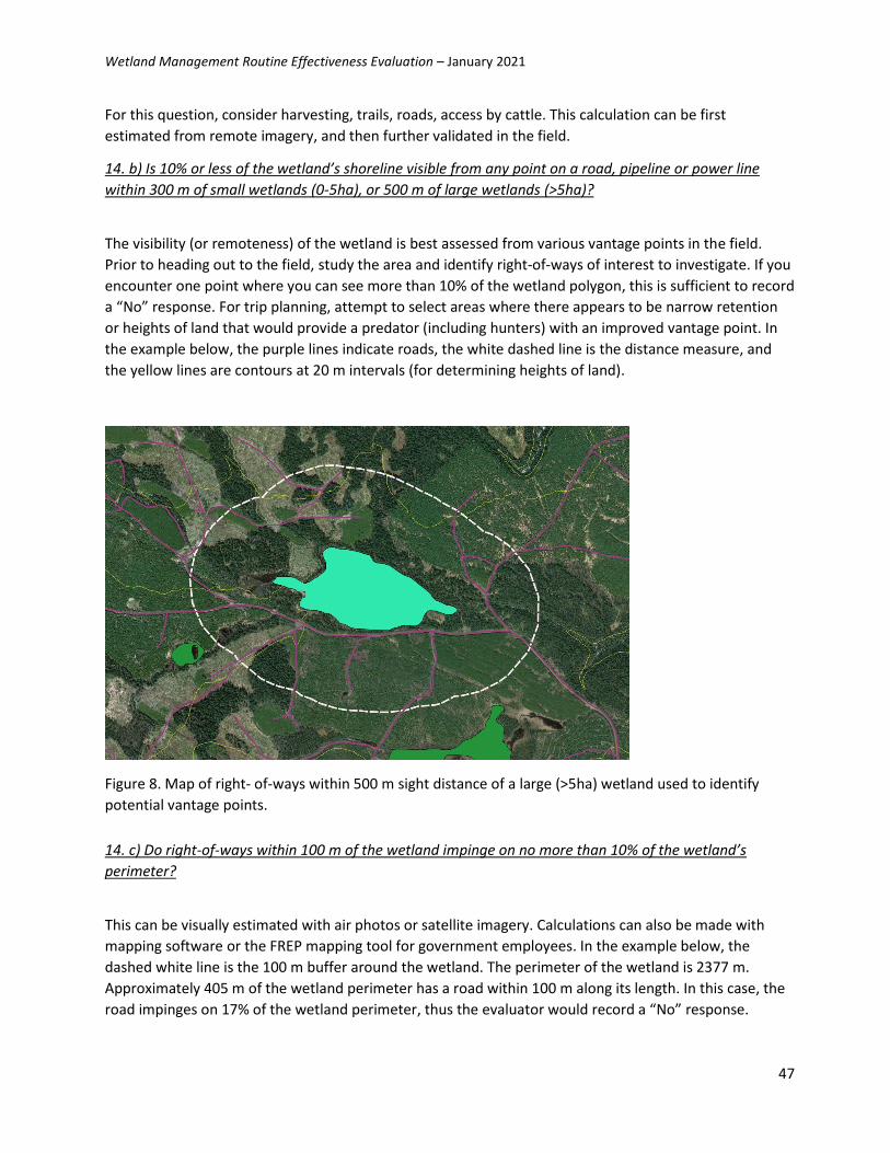
Wetland Management Routine Effectiveness Evaluation – January 2021
47
For this question, consider harvesting, trails, roads, access by cattle. This calculation can be first
estimated from remote imagery, and then further validated in the field.
14. b) Is 10% or less of the wetland’s shoreline visible from any point on a road, pipeline or power line
within 300 m of small wetlands (0-5ha), or 500 m of large wetlands (>5ha)?
The visibility (or remoteness) of the wetland is best assessed from various vantage points in the field.
Prior to heading out to the field, study the area and identify right-of-ways of interest to investigate. If you
encounter one point where you can see more than 10% of the wetland polygon, this is sufficient to record
a “No” response. For trip planning, attempt to select areas where there appears to be narrow retention
or heights of land that would provide a predator (including hunters) with an improved vantage point. In
the example below, the purple lines indicate roads, the white dashed line is the distance measure, and
the yellow lines are contours at 20 m intervals (for determining heights of land).
Figure 8. Map of right- of-ways within 500 m sight distance of a large (>5ha) wetland used to identify
potential vantage points.
14. c) Do right-of-ways within 100 m of the wetland impinge on no more than 10% of the wetland’s
perimeter?
This can be visually estimated with air photos or satellite imagery. Calculations can also be made with
mapping software or the FREP mapping tool for government employees. In the example below, the
dashed white line is the 100 m buffer around the wetland. The perimeter of the wetland is 2377 m.
Approximately 405 m of the wetland perimeter has a road within 100 m along its length. In this case, the
road impinges on 17% of the wetland perimeter, thus the evaluator would record a “No” response.

Wetland Management Routine Effectiveness Evaluation – January 2021
48
Figure 9. Example of road impinging within 100 m of wetland area along the southwest (Q 14c).
14. d) Is the percent of mature and old forest within two kilometers of the wetland perimeter greater than
the minimal target for the area’s biogeoclimatic zone and natural disturbance type?
Landscape connectivity helps provide wildlife with sufficient and different habitat types to adequately
meet their life needs. Gaps in connectivity can increase risk of predation, reduce suitable habitat, and
ultimately limit chances of survival. The amount of intact habitat required can vary among species. The
following indicator was adapted from a broadly utilized methodology in North America to estimate
landscape connectivity around wetlands and other landscape features of interest. A similar methodology
is utilized by the Conservation Data Centre of BC. This FREP wetland health evaluation applies a threshold
of percent of mature and old forests that surround a wetland as a proxy of landscape connectivity. The
targeted percent of mature and old forest varies by the site’s natural disturbance regime and
biogeoclimatic zone. Appendix 4 provides the minimum targets.
This indicator is best completed as a desktop exercise utilizing the best available wetland polygon that
delineates the wetland boundaries.
Steps:
1. Place a 2000 m (2 km) spatial analysis buffer around the wetland.
2. Estimate the percent of old and mature forests within the buffer. Tip: If you have access to GIS
software (e.g., QGIS), you can run a query on the Vegetation Resource Inventory spatial layer.
Select or extract polygons within the fields: Forest Management Land Base
“FOR_MGMT_LAND_BASE_IND” == Y and that have an age “PROJ_AGE_1” greater than the
targeted age. For government employes, this can be achieved using the filter and VRI reporting

Wetland Management Routine Effectiveness Evaluation – January 2021
49
widgets in FREPmap. For targets, use the table in Appendix 4 based on the wetland’s dominant
biogeoclimatic zone and natural disturbance type. If you don’t have access or the ability to
conduct this type of spatial analyses, an estimate using aerial imagery and any other supporting
information is sufficient.
3. Calculate the proportion of the polygon that meets the criteria.
Figure 10. Example of a spatial query for mature and old forests within a 2 km buffer of the wetland.
In the example shown in Figure 10, the wetland is within a natural disturbance type NDT3 and the
biogeoclimatic zone and variant is SBSmc2. From the table in Appendix 4, the target mature and old
forest is greater than 34%, and the minimal age is 100 years. The proportion of polygons meeting these
criteria is 47.6% of the forest land base, therefore the wetland has sufficient mature and old forest.
15. Are surface and subsurface flows to the wetland intact?
Roads and other right-of-ways (ROWs) can have a significant impact on wetlands by diverting the flow of
both surface and shallow ground water. The following questions are coarse-level indicators of potential
impacts.
15.a) Do all mapped and unmapped streams at roads and ROWs appear to be in their original water
courses?
Field surveyors should drive or otherwise traverse the roads and ROWs upslope of the wetland whenever
possible. If available, this evaluation can be conducted using drone imagery. Look for mapped and
unmapped streams and groundwater exposures where there have been cuts. Unmapped streams or
groundwater exposures (i.e., new springs) are typically not part of the planning phase and may contribute
significantly to changes in water inputs. If surface water is diverted upslope and away from its original
trajectory (i.e., not provided with sufficient passage through a culvert or bridge), record “No”. Look for

Wetland Management Routine Effectiveness Evaluation – January 2021
50
drainage ditches alongside the road; look for flowing water, or evidence of flow, that suggests water is
taken away from its natural course. If the wetland is adjacent to a lake or a river, only evaluate the face
drainage that enters the wetland and not the drainage for the entire lake or river.
15.b) Is less than 25% of the contributing basin intercepted by roads or ROWs?
This is a map-based exercise that is best initiated before the field visit. It requires the use of topographic
maps to estimate the hydrology and road layers. Record the amount of the basin that is separated from
the wetland by a ROW.
If the surveyor observes additional roads or ROWs that were not on the map, the surveyor needs to draw
in/digitize the location of this missing road on the map and re-calculate the percentage of the wetland
drainage area potentially affected.
The contributing basin is the land where surface waters would flow into the wetland via streams or sheet
flow on the surface or subsurface. First, estimate the area of the contributing basin on a map by
interpreting surrounding streams and elevation contour lines or hill shade imagery. Next, estimate the
amount of the contributing basin intercepted by ROWs.
Example: The white area in Figure 11a is a predefined sub-watershed area from the BC Freshwater Atlas.
The light pink polygon is the approximate contributing basin for the wetland (light blue/green polygon).
Both streams (blue lines) and contour lines (brown lines) were used to approximate the contributing
basin. The areas within the contributing basin intercepted by roads (black lines) is displayed as dark pink
in Figure 11b. In this example 501 out of 631 hectares are intercepted by right of ways (i.e., 79%).
Figure 11. A) Contributing basin shown as polygon in light pink; B) polygon with flow intercepted by ROW
in dark pink.
A B

Wetland Management Routine Effectiveness Evaluation – January 2021
51
Appendix 1 – Recommended Field Sampling Sequence
Introduction:
Steps 1 through 4 describe the process for completing your transect. However, there are other tables that have
“continuous” information – you will fill these tables out AFTER you’ve completed all your transects. It’s helpful to
mentally record, take photos, or start tallies (as appropriate), so that you can recollect what you’ve seen.
Continuous tables include:
o T.5.3. Bare Ground Hydrologically Connected to the wetland
o T. 6. Structural features missing or impacted within 10 m upland from wetland edge, and the condition of
those features (the Form, Vigor and Recruitment)
o T.7.2. Distribution Code of Invasive Species
o T. 7.3 Observations about the Diversity of Decay and Size Classes of Snags and Coarse Woody Debris
o T.7.4. Impacts to vegetation (i.e., impacts that may prevent the vegetation community from achieving
it’s climax community, pressures from overgrazing/browsing)
o T. 8. Structural features missing or impacted within the wetland, and the condition of those features (the
Form, Vigor and Recruitment)
o T. 9. Physical and Hydrological Impacts to the Wetland. Take a moment to review questions within this
table. Ensure you have an opportunity to assess the outlet, inlet, and any significant channel that is
within the wetland.
o In addition, while approaching your sampling location, or walking around the wetland, observe any
anomalies that are significant stressors that may be located outside of your transect (i.e., large patches of
bare soil, invasive plants, disturbance/increaser species, low retention within RMZ or high disturbance in
RMA, harvesting in wetland, dead or decadent trees, excessive windthrow or newly deposited coarse
woody debris). Record anomalies that may affect your overall score in the second last column of Table
5.1 and Table 7.1, titled: “Large non-homogenous patches outside transect but within upland
area/assessment polygon”.
Step 1. At your sampling location, mark edge of wetland boundary with flagging tape. Record UTM Coordinates
in T.4.1., you will fill out other columns in this table later.
Step 2. Run a transect line upland from the wetland edge, and mark 10 m & 20m upland perpendicular from
wetland edge with flagging tape. While you have your transect line laid out and you are exploring your upland
location:
o In Table 4.3., document invasive or disturbance species within the first 10 m upland from wetland edge.
Make % estimates based on 10 m on either side of the transect line.
o In Table T.5.1., there are 3 columns labeled T1-T3, one for each transect you will sample. Complete a
transect column. Make % estimates based on 10 m on either side of the transect line for Question
Indicators 3 and 5.
o Table T.7.1. is completed based on the full transect length (i.e., 10 m upland plus wetland observations).
Mentally take note of question indicators 1 to 9a in T.7.1.
o Start recording old (O) and new (N) coarse woody debris that cross your transect line (i.e., Question
Indicator 9c) in T.7.1. Note: if woody debris extends into the wetland you will need to continue recording
CWD once you extend your transect into the wetland (Step 4). While observing coarse woody debris,
also check off the decay class and diameter class in T.7.3. Once you’ve checked off a decay class or
diameter range, you don’t need to check off the same class or diameter range again (this is a continuous
observation).
o If there is new windthrow (since disturbance), then also begin to make a tally for Question Indicators
10a,b. in T.5.2. Note: consider 20 m upland from wetland edge for wetlands without an RRZ, and 10 m
upland from wetland edge for wetlands with an RRZ.

Wetland Management Routine Effectiveness Evaluation – January 2021
52
o In Table 7.3. also check off the decay and diameter classes of snags (dead standing trees) 10 m on either
side of you.
o Reel in your rotary tape. You will now explore the wetland.
Step 3. Run a transect line into the wetland that is perpendicular from the wetland perimeter. One of the crew
members may stand on the edge of the wetland perimeter to guide the other into the wetland on a compass
bearing and to help record notes.
o In Table 4.1. document the transect bearing, end type (e.g., end of 50 m, channel, etc.), and Transect
Length. Add 10 m to account for the upland portion. If you are entering a new wetland plant community
at the end of your transect, then you may also add an additional 10 m to the transect length on the
other end so that you can incorporate your observations of this new plant community (this may occur if
you encounter, for instance, Shallow Open Water and are unable to walk further). Once you reach the
extent of the transect, leave the rotary tape laid out. Remember that your transect represents one side
of your wetland. Your transect length cannot be closer to any other part of the wetland perimeter than
from where you placed your flagging tape for this transect at the wetland edge (Otherwise you are
recording observations that are likely influenced from a different edge of the wetland).
o Continue recording old (O) and new (N) coarse woody debris that cross your transect line (i.e., Question
Indicator 9c) in T.7.1. While observing coarse woody debris, also check off the decay class and diameter
class in T.7.3.
o If there is new windthrow (since disturbance), then continue to make a tally for Question Indicators
10a,b,c. in T.7.1.
o In Table 7.3., check off the decay and diameter classes of snags (dead standing trees) 10 m on either side
of you.
o Complete plots within each distinct vegetation zone. Fill out Table 4.2 (a row per plot) and Table 4.3
concurrently. While completing Table 4.3, only record: dominant native species in addition to invasive
species. An exhaustive list is not necessary for this assessment. If you cannot identify a species, then
make a quick note (e.g., Salix Sp.?), record percent cover, and then move on! This portion of the
assessment should be quick. Dominant species should help you classify your wetland. If you are not
confident about the wetland class or plant association, then leave it blank in T.2. You will still be able to
assess your site. Along the length of the transect make observations either 10 m from the plot centre,
OR if the band of vegetation is narrower than 20 m, then to the extent of the vegetation zone where
there is a distinct break. Make observations 10 m on either side of the transect line. The intent is only
to document observations that represent the vegetation zone you are trying to describe.
o After you’ve completed the plots on your transect, complete the rest of your transect information (i.e.,
column T1,T2, or T3) in T.7.1., taking into account observations you made from the 10 m upland portion
plus what you observed along the transect in your wetland portion. Imagine the transect as one strip
that is 20 m wide (10 m on either side)
Step 4. Repeat steps 1 through 3 until you’ve completed all your transects.
Step 5. Fill out the Continuous Tables as described at the introduction of this document.
Step 6. Complete the remainder of T.4.1. (i.e., the fractional information in the last 3 columns)
Step 7. Complete the weighted averages in T.5.1 by using weights recorded as Fb in Table 4.1. Then add
percentages from transects and anomalies in the last column.
Step 8. Complete the weighted averages in T.7.1. by using weights recorded as WF in Table 4.1 for question
indicators 1 to 9a. Then add percentages from transects and anomalies in the last column.
Step 9. Fill out pages 12 to 15 based on your records.
Step 10. Summarize your findings, score your wetland, and document causal factors on page 16 and 17
Step 11. Prepare a small map that shows your transects and key features within your wetland on page 18.

Wetland Management Routine Effectiveness Evaluation – January 2021
53
Appendix 2 – Common Invasive and Noxious Plants in BC
Invasive/Noxious Plant Species1 Scientific Name Wetland Indicator Status2
Page Number3
Anchusa (Common Bugloss) Anchusa officinalis pNA, P50
Baby's Breath Gypsophila paniculata p320, P73
Black Knapweed Centaurea nigra pNA, PNA
Blueweed Echium vulgare p76, P47
Bohemian Knotweed Fallopia x bohemica P26
Brazilian Waterweed (syn. Brazilian Eloda)
Egeria densa OBL PNA
Brown Knapweed Centaurea jacea FACU pNA, PNA
Buck’s-horn Plantain Plantago coronopus FACW PNA
Bull Thistle Cirsium vulgare FACU pNA, P75
Canada Thistle Cirsium arvense FACU p32, P9
Caulerpa Caulerpa taxifolia PNA
Common Burdock Arctium minus FACU pNA, P48
Common Tansy Tanacetum vulgare FACU p58, P51
Cordgrass Spartina spp. OBL/FAC P11-14
Creeping Buttercup Ranunculus repens L. FAC P79
Dalmation Toadflax Linaria dalmatica p136, P6
Dandelion Taraxacum PNA
Didymo Didymosphenia geminata OBL PNA
Diffuse Knapweed Centaurea diffusa P29, P74
Dwarf Eelgrass Zostera japonica FACU PNA
Eurasian Watermilfoil Myriophyllum spicatum OBL PNA
European Common Reed Phragmites australis spp OBL P10
Fanwort Cabomba aquatica PNA
Field Scabious Knautia arvense P382, P52
Flowering Rush Butomus umbellatus FACW/OBL P17
Giant Hogweed Heracleum mantegazzianum FAC P19
Giant Knotweed Fallopia sachalinensis FACU PNA, P27
Giant Mannagrass/Reed Sweetgrass Glyceria maxima OBL P20
Giant Reed Arundo donax PNA
Gorse Ulex europaeus FACU pNA, P21

Wetland Management Routine Effectiveness Evaluation – January 2021
54
Hairy Willow Herb Epilobium hirsutum FACW PNA
Hanging Sedge Carex pendula PNA
Himalayan Balsam (syn. Policeman’s Helmet)
Impatiens glandulifera FACW P84
Himalayan Knotweed Persicaria wallichii FAC P28
Hoary Alyssum Berteroa incana pNA, P55
Hoary Cress Cardaria draba P272, P56
Hound's-tongue Cynoglossum officinale FACU pNA, 22
Hydrilla Hydrilla verticillata PNA
Japanese Knotweed Fallopia japonica FACU p91, P29
Japanese Wireweed Sargassum muticum P84
Leafy Spurge Euphorbia esula p368, P30
Marsh Plume Thistle Cirsium palustre pNA, P60
Meadow Hawkweed Hieracium caespitosum pNA, PNA
Meadow Knapweed Centaurea debeauxii pNA, P57
Nodding Thistle Carduus nutans FACU p26, P87
Orange Hawkweed Hieracium aurantiacum p40, P54
Oxeye Daisy Leucanthemum vulgare FACU p30, P62
Parrots Feather Myriophyllum aquaticum OBL PNA
Perennial Pepperweed Lepidium latifolium FAC pNA, P63
Plumeless Thistle Carduus acanthoides p27, P67
Poison Hemlock Conium maculatum FACW PNA
Policeman's Helmet Impatiens glandulifera FACW PNA
Puncture Vine Tribulus terrestris p96, P64
Purple Loosestrife Lythrum salicaria FACW p224, P35
Reed Canary Grass Phalaris arundinacea FACU PNA
Rush Skeletonweed Chondrilla juncea pNA, P36
Russian Knapweed Acroptilon repens pNA, P58
Russian Olive Elaeagnus angustifolia FAC PNA
Scentless Chamomile Matricaria maritima p48, P37
Scotch Broom Cystisus scoparius pNA, P88
Scotch Thistle Onopordum acanthium pNA, P69
Spotted Knapweed Centaurea biebersteinii p28, P25
St. John's Wort Hypericum perforatum FACU pNA, P89
Sulphur Cinquefoil Potentilla recta p357, P66
Swollen Bladderwort Utricularia inflata OBL PNA

Wetland Management Routine Effectiveness Evaluation – January 2021
55
Tansy Ragwort Senecio jacobaea FACU p59, P39
Teasel Dipsacus fullonum FAC pNA, P90
Variable-leaf Milfoil Myriophyllum heterophyllum PNA
Wakame Undaria pinnatifida PNA
Water Primrose Ludwigia hexapetala PNA
Wild Chervil Anthriscus sylvestris P70
Wild Parsnip Pastinaca sativa PNA
Yellow Flag Iris Iris pseudacorus OBL pNA, PNA
Yellow Floating Heart Nymphoides peltata OBL PNA
Yellow Nut Sedge Cyperus esculentus FACW P34
Yellow Starthistle Centaurea solstitialis p29, P45
Yellow Toadflax Linaria vulgaris p138, P40 1Sources for selected plant list: BC Wildlife Federation. 2015. Priority Aquatic Invasive Plants in BC.
Factsheet. Invasive Species Council of BC. Personal Communication (March 2018).
2 Page numbers following a lower case ‘p’ are given for the descriptions found in Weeds of Canada. 1999.
Royer and Dickerson. Lone Pine Publishing and The University of Alberta Press. Page numbers following an
uppercase ‘P’ are from the Field Guide to Noxious Weeds and Other Selected Invasive Plants of British
Columbia. 2014. Cranston, et al. British Columbia.
3Sources for Wetland Indicator Status: United States Department of Agriculture. 2018. Plants Database.
Wetland Indicator Status. https://plants.usda.gov/wetinfo.html; and W.H. MacKenzie and J.R. Moran.
2004. Wetlands of British Columbia: A Guide to Identification. Res. Br., B.C. Min For., Victoria, B.C. Land
Manage. Handb. No. 52.

Wetland Management Routine Effectiveness Evaluation – January 2021
56
Appendix 3 – Select List of Culturally Significant Plants to Indigenous Communities in BC
Species Name Common Name Class
Alnus rubra Bong. red alder FACU
Angelica genuflexa Nutt. kneeling angelica FACW
Apocynum cannabinum L. Indian hemp FAC
Argentina anserina (L.) Rydb. (syn. Potentilla anserinaL common silverweed FACU
Argentina egedii (Wormsk.) Rydb. (syn. Potentilla egedii Wormsk.) Pacific silverweed FACW
Athyrium filix-femina (L.) Roth. ssp. cyclosorum (Rupr.) C. Chr. common ladyfern FACU
Betula nana L. scrub birch (syn. Betula glandulosaMichx.) FACU
Betula occidentalis Hook. water birch FACW
Betula pumila var. glandulifera Regel bog birch OBL
C. virosa L. Mackenzie’s water-hemlock FACW
Camassia quamash (Pursh) Greene common camas FACW
Carexobnupta L.H. Bailey slough sedge FACW
Chamaecyparis nootkatensis (D. Don) Spach (syn. Cupressus nootkatensis D. Don) Yellow cedar FAC
Cicuta douglasii (DC.) J.M. Coult. & Rose Douglas’ water-hemlock FACW
Comarum palustre L. purple marshlocks OBL
Conocephalum conicum (L.) cone-headed liverwort
Cornus sericea L. (syn. Cornus stolonifera) red-osier dogwood, or “red willow” FACU
D. anglica Huds. English sundew OBL
Drosera rotundi folia L. Round leaved sundew OBL
Elaeagnus commutata Bernh. ex Rydb silverberry FAC
Empetrum nigrum L. black crowberry, “blackberry” FACU
Equisetum arvense L. common, or field horsetail FACU
Equisetum hyemale L. ssp. affine scouring rush, or branchless horsetail FACW
Equisetum telmateia Ehrh. giant horsetail FACW
Eriophorum angustifolium Honck., and E. chamissonis C.A. May. cottongrass OBL

Wetland Management Routine Effectiveness Evaluation – January 2021
57
Frangula purshiana (DC.) Cooper (syn. Rhamnus purshiana DC.) cascara FAC
Fritillaria camschatcensis (L.) Ker Gawl. northern rice-root FACW
Hierochloe hirta (Schrank) Borbás northern sweetgrass FACW
Juniperus communis L. common juniper FACU
Kalmia microphylla (Hook.) A. Heller; syn. Kalmia polifolia Wangenh. bog laurel, or swamp-laurel OBL
Kamchatka fritillaria sarana lily FACW/OBL
Labrador-tea, and R. neoglandulosum Harmaja (syn. L. glandulosum Nutt.) (syn. Rhododendron groenlandicum) trapper’s tea, or western Labrador tea FACU
Ligusticumcanbyi (J.M. Coult. & Rose) J.M. Coult. & Rose Canby's lovage or Canby’s licorice-root FAC
Lonicera involucrate (Richardson) Banks ex Spreng.
black twinberry or twinberry honeysuckle FACU
Lupinus nootkatensis Donn ex Sims Nootka lupine FACU
Lycopus uniflorus bugleweed OBL
Lysichiton americanus Hultén& H. St. John American skunk-cabbage FACW
Malus fusca (Raf.) C.K. Schneid. Pacific crabapple FACU
Mentha arvensis L. field mint or Canada mint FACU
Myrica gale L. sweetgale OBL
Nuphar lutea (L.) Sm. ssp. Polysepala (Engelm.) E.O. Beal yellow water-lily OBL
Oenanthe sarmentosa C. Presl ex DC. Water parsley OBL
Populus balsamifera ssp. trichocarpa (Torr. & A. Gray ex Hook.) Brayshaw black cottonwood FAC
Platanthera hyperborean (L.) Lindl. (syn Platanthera aquilonis) northern green orchid FACW
Physocarpus malvaceus (Greene) Kuntze mallow ninebark Not listed
Platanthera stricta Lindl. slender bog orchid FACW
Phalaris arundinacea L. reed canary grass FACU

Wetland Management Routine Effectiveness Evaluation – January 2021
58
Phragmites australis (Cav.) Trin. Ex. Steud. common reed grass and related spp. OBL
Physocarpus capitatus (Pursh) Kuntze Pacific ninebark FACU
Picea mariana (Mill.) Britton, Sterns &Poggenb. black spruce FACU
Pinus contorta Douglas ex Louden lodgepole pine FACU
Platanthera dilatate (Pursh) Lindl. ex Beck white bog orchid FACW
Populus balsamifera L. ssp. balsamifera balsam poplar FAC
Potamogeton natans L. floating pondweed OBL
Rhododendron groenlandicum (Oeder) K.A. Kron & W.S. Judd (syn. Ledum groenlandicum Oeder) Labrador-tea FACW
Ribes bracteosum Douglas ex Hook. gray currant or stink currant FACU
Rubus arcticus L. ssp. Acaulis (Michx.) Focke Nagoonberry or dwarf raspberry FACW
Rubus chamaemorus L. cloudberry or bakeapple OBL
Rubus spectabilis Pursh salmonberry FACU
Rumex aquaticus L. var. fenestratus (Greene) Dorn (syn. Rumex occidentalis S. Watson) western dock FACW
Salix bebbiana Sarg. Bebb’s willow FACU
Sagittaria cuneate Sheldon arumleaf arrowhead OBL
Salix discolor Muhl. pussy willow FACW
Salix hookeriana Barratt ex Hook. Hooker’s willow FACW
Schoenoplectus lacustris (L.) Palla [syn. S.tabernaemontani (C.C. Gmel.) Palla] lakeshore bulrush or softstem bulrush OBL
Salix scouleriana Barratt ex Hook. Scouler’s willow FAC
Sorbus sitchensis Sanson ex Bong. Sitka mountain ash FAC
Sagittaria latifolia Willd. wapato, or broadleaf arrowhead OBL
Salix barclayi Andersson Barclay’s willow and other mountain willows FACU
Salix exigua Nutt. sandbar willow, or rope willow FACW
Salix lucida Muhl. ssp. lasiandra (Benth.) E. Murray Pacific willow FACW
Sambucus racemosa L. red elderberry FACU

Wetland Management Routine Effectiveness Evaluation – January 2021
59
Schoenoplectus acutus (Muhl. ex Bigelow) A. Löve & D. Löve hardstem bulrush OBL
Schoenoplectus americanus (Pers.) Volkart ex Schinz & R. Keller (syn. Scirpusolneyi A. Gray) Olney’s three-square bulrush FACW
Scirpus microcarpus J. Presl & C. Presl small-flowered bulrush or “cut-grass” OBL
Sium suave Walter Water parsnip OBL
Sphagnum spp. Sphagnum moss or peat moss (several species) OBL
Spiraea douglasii Hook. hardhack FACW
Stachys chamissonis Benth. var. cooleyae (A. Heller) G. Mulligan & D. Munro coastal hedge-nettle OBL
Taxus brevifolia Nutt. Pacific yew or western yew FACU
Thuja plicata Donn ex D. Don western redcedar FACU
Tricholoma populinum Lange cottonwood mushroom Not listed
Trifolium wormskioldii Lehm. springbank clover FACW
Triglochin maritima L. seaside arrowgrass OBL
Typha latifolia L. cattail OBL
Viburnum. opulus L. American highbush cranberry or bush cranberry FACW
Vaccinium oxycoccos L. bog cranberry or small cranberry OBL
Vaccinium uliginosum L. bog bilberry FACU
Vaccinium vitis-idaea L. lingonberry or lowbush cranberry FACU
Veratrum viride Aiton false hellebore, or green false hellebore FACU
Viburnum edule (Michx.) Raf. highbush cranberry or squashberry FACU Sources: Turner, Nancy J. Food plants of coastal first peoples. Victoria: Royal BC Museum, 2010. Print.
Turner, Nancy J. Food plants of interior first peoples. Victoria: Royal BC Museum, 2007. Print.

Wetland Management Routine Effectiveness Evaluation – January 2021
60
Appendix 4 – Wetland Indicator Status Categories
Indicator Code Indicator Status Designation Comment
OBL Obligate Wetland Hydrophyte Almost always occur in wetlands.
FACW Facultative Wetland Hydrophyte Usually occur in wetlands but may occur in non-wetlands.
FAC Facultative Hydrophyte Occur in wetlands and non-wetlands.
FACU Facultative Upland Non-hydrophyte Usually occur in non-wetlands but may occur in wetlands.
UPL Obligate Upland Non-hydrophyte Almost never occur in wetlands.
Source: United States Department of Agriculture. 2018. Plants Database. Wetland Indicator Status.
https://plants.usda.gov/wetinfo.html

Wetland Management Routine Effectiveness Evaluation – January 2021
61
Appendix 5 Minimal Targets for Mature and Old Forest Coverage___________________
Natural
Disturbance
Type BEC & Variant
Upland-Wetland
Objective
Minimal % Target
for Mature + Old Minimal Age
NDT1
CWH High 54 80
ICH High 51 100
ESSF High 54 120
MH High 54 120
NDT2
CWH Mod 34 80
CDF Mod 34 80
ICH Mod 31 100
SBS Mod 31 100
ESSF Mod 28 120
SWB Mod 28 120
NDT3
SBPS Low 8 100
SBSdk Low 11 100
SBSdw Low 11 100
SBSmk Low 11 100
SBSmc3 Low 11 100
SBSwk1 Low 11 100
SBS - other High 34 100
BWBSmw Low 11 80/100*
BWBSdk Low 11 80/100*
BWBSwk Low 11 80/100*
BWBS - other High 34 80/100*
MS - other High 39 100
MSxv moderate-high 26 100
ESSF High 34 120
ICH High 34 100
CWH High 34 80
NDT4
ICH high 51 100
IDFdk moderate-high 34 100
IDF - other high 51 100
PP high 51 100 *For BWBS, the minimal target age is 80 years for deciduous prominent & 100 years for coniferous prominent.
Source: Parminter, J. 1995. Biodiversity Guidebook. Forest Practices Code of British Columbia. B.C. Min. For. and B.C.
Environ., Victoria, B.C.