EVALUATING PURCHASING POWER PARITY IN ... - …ijecm.co.uk/wp-content/uploads/2015/01/311.pdf ·...

International Journal of Economics, Commerce and Management United Kingdom Vol. III, Issue 1, Jan 2015

Licensed under Creative Common

http://ijecm.co.uk/ ISSN 2348 0386

EVALUATING PURCHASING POWER PARITY IN

HYPERINFLATION AND LOW INFLATION COUNTRIES

A CASE OF STRUCTURAL BREAKS

Karen Oseikhuemen Ikhifa-Aigbokhan

Queen Mary University of London, United Kingdom

[email protected]

Abstract

The theory of purchasing power parity has continually been evaluated over the years using

different approaches that could be in favour of the theory. Some studies have obtained data

from low-inflation and high-inflation countries to test for the theory. In this study, ADF and KPSS

tests are employed, testing for unit root of 5 countries’ effective exchange rate, in which they are

split into hyperinflation and low inflation countries. Other tests such as the Bai-Perron test are

employed to test for structural breaks over time. In contrast to previous studies that used the

CPI and WPI, this study finds that PPP is not valid in both hyperinflation and low inflation

countries. This therefore infers that PPP is not suitable for exchange rate determination in these

economies.

Keywords: PPP, KPSS, ADF, Effective Exchange Rates, Inflation, Structural Breaks.

INTRODUCTION

“The willingness to pay a certain amount for foreign money must ultimately and essent ially be

due to the fact that this money possesses a purchasing power against goods and services in

that country; on the other hand, when so much of our money is offered, we are actually offering

purchasing power parity against goods and services in our own country. Our valuation of a

foreign currency in terms of our own currency depends on the relative purchasing power of both

currencies in their various countries” (Cassel 1922 in Taylor and Taylor 2004, pp.135)”. The

theory of purchasing power parity was first examined by David Ricardo; however, Gustav

Cassel made the theory popular in 1918 when he termed it the purchasing power parity theory.

Cassel who studied international trade explain that purchasing power parity doctrine suggests

http://ijecm.co.uk/

© Karen


that identical goods from different countries should sell at same price when converted to one

currency. The theory was made popular during the World War I, evaluating the purchasing

power of currencies between different countries. Although theoretical framework supports that

purchasing power parity holds, most empirical work have proven otherwise. PPP hypothesis

demonstrates that domestic and foreign price ratios are equivalent when converted to the same

currency. Balassa (1964) explains the two versions of purchasing power parity namely the

Absolute PPP doctrine and the Relative PPP doctrine. He states that Absolute PPP doctrine is

based on the price ratio of consumer goods for any pair of countries and it is approximated to

the exchange rate equilibrium while on Relative PPP doctrine, he states that when the

exchange equilibrium prevails, changes in prices would show shifts in exchange rate. Some

studies have failed to reject null hypothesis and also suggest that there may be deviations in the

short run causing PPP not to hold and the tendency for mean reversion in exchange rate, but

this may not be the case in the long run as exchange rate meets at equilibrium. Past studies

also infer that testing for the validity of PPP using bilateral exchange rate may not favour the

theory. Tests such as the Augmented Dickey-Fuller test has been used to test for unit root but

has been criticised owing to the fact that it often fails to reject null hypothesis. The KPSS test

which has recently been introduced is used alongside with the ADF test by some researchers

and is sometimes able to reject null hypothesis. Further studies suggest that structural changes

in the economy have effects on purchasing power between countries. Testing for structural

changes, the Chow test and recently introduced Bai-Perron tests are used. However, there is

limitation in the use of the chow test due to need that break dates are specified before the test is

done, although, it still often times provides accurate results.

Furthermore, due to the lack of consensus on the validity of PPP theory, this study

attempts to further test the conflicting conclusion. In this paper, the theory is evaluated using the

Effective Exchange Rate and Consumer Price Index (CPI) and Wholesale Price Index (WPI).

This paper aims at verifying if PPP holds in Argentina, Australia, Canada, Japan and USA with

USA being a low inflation country, therefore is the home country; also, testing for PPP in a high

inflation country, Argentina is used as the home country with Canada, Australia and Japan as its

trading partners. Although, some studies have argued that estimating the wholesale price index

rather than the consumer price index shows more evidence in favour of PPP. To verify the

authenticity of this argument, this paper will be evaluating PPP using the wholesale price index

as well. In addition, there is no clear possibility that PPP may hold using the WPI. Although, WPI

may have more weight than CPI, still, it should be noted that WPI is based on specific type of

goods in specified regions; this makes the possibility that using WPI may favour some countries

than others, in other words, it may not favour PPP.

International Journal of Economics, Commerce and Management, United Kingdom


The paper is structured as follows: Chapter 2 reviews the literature behind the purchasing power

parity doctrine and the law of one price as a core aspect of PPP. Chapter 3 describes the data

collected and the methodology used. Chapter 4 presents and explains empirical results based

on tests carried out. Chapter 5 summarises the main findings and offers a conclusion.

LITERATURE REVIEW

Continuous and extensive research has been carried out on purchasing power parity in the

short-run, medium-run and long-run. Purchasing Power Parity (PPP) theory is based on traded

goods only and it is another concept of the Law of One Price (LOOP); the PPP theory states

that the price of goods in Country A must be the same price of goods in Country B when

converted to the same exchange rate, where both goods are identical. The relationship between

economic sine qua non and exchange rate behaviour has been a controversial issue in

international finance, showing various empirical puzzles such as the purchasing power parity

(Chen and Rogoff2002).

Abuaf and Jorion (1990) and Yin-Wong andKon (1993) explain that the purchasing

power parity (PPP) doctrine is a fundamental basis of exchange rate determination. Farooq

(2006) asserts that PPP doctrine implies an even restriction on domestic and foreign prices in a

long-nominal exchange rate equation; in which he further argues that these restrictions are

enacted by real exchange rate definition. According to Yin-Wong and Kon (1994) “PPP theory

suggest that currencies are valued for the goods they can purchase and, in arbitrage

equilibrium, the exchange rate between two countries‟ currencies should equal the ratio of their

price levels, of which a testable implication is that real exchange rate should display mean

reversion, at least in the long-run”. In Frenkel (1981) view, there is contention behind the

usefulness of the purchasing power theory; owing to the fact that there is no specified

mechanism by which the exchange rate and prices are linked neither does it specify the

conditions in which the PPP theory is satisfied.

“The idea that purchasing power parity may hold because international goods arbitrage

is related to the so-called L aw of One Price, which holds that the price of an internationally

traded good should be the same anywhere in the world once the price is expressed in the same

currency, since people could make a riskless profit by shipping the goods from locations where

the price is low to locations where the price is high (arbitraging) Taylor and Taylor (2004)”.

According to Rogoff (1996), the variants of PPP are Law of One Price, Relative PPP and

Absolute PPP and the Indices of measuring Absolute PPP; he emphasises that the issue of

arbitrage in relation to LOOP was put in place, that is, the idea that if goods market arbitrage

leads to an extensive parity in prices across a large scope of individual goods which is the law

© Karen


of one price, then there should also be a relationship in aggregate price levels. Research carried

out using the „Big Mac‟ hamburgers as an illustration is to explain the Law of One Price. The

Law of One Price theory states that the price of a given commodity or product should be the

same price when changed to different currency between countries. However, this is not often

the case. Using the Big Mac prices in 10 countries, Table 1 shows the prices of MacDonald

burger in the 10 different countries; Switzerland has the highest price of burger selling at $7.14

while Hong Kong has the least price of burger which sells at $2.32.

TABLE 1 Relative Prices of Big Mac across some Counties

Country Prices of Big Mac (in dollars)

Australia 4.47

Canada 5.01

China 2.74

Denmark 5.18

Euro Area 4.96

Germany 4.98

Hong Kong 2.32

Japan 2.97

Switzerland 7.14

United States 4.62

Source: The Economist, June, 2014.

This difference in the price of same good in different countries may lead to the question as to

why there is price difference among countries. Rogoff (1996) however explains that non-traded

inputs may not be the main reason for differences in prices, Value Added Tax (VAT) may also

contribute to violation of LOOP; he further demonstrates his arguments by giving an example,

that is, in the United States and Canada, ketchup for hamburger is free but in Italy and Holland,

it costs extra cents. The presence of transaction costs, transportation costs, taxes, tariffs, non-

tariff barriers and other commission costs would encourage a violation of LOOP says Taylor and

Taylor (2004). Also, the difference in the relative productivity and the relative size of the public

sector further contributes to the violation (Pakkio and Pollard 2003).

Rogoff (1996) explain that another way of measuring PPP is to employ the Absolute

PPP which requires that sums are taken over a Consumer Price Index (CPI); knowing that the

sum of price of goods in home country is the same as the sum of price of goods in another

country. There is however acquisition as to which consumer price index, if it is home or foreign,

and the problem associated with trying to implement absolute purchasing power parity, is the

little or no available data used in measuring it. Relative PPP on the other hand requires only that



the growth rate in the exchange rate equipoise the discrepancy between the growth rate in

home and foreign price levels. Explaining the versions of PPP which may not hold using

aggregate price levels with reference to monetary shocks, Frenkel (1981) states that the

relationship between exchange rate and to price levels and exchange rate to inflationary

differentials are likely to hold if the internal relative prices are stable when there are monetary

shocks; although if the relative prices change then PPP may not be valid.

Previous research carried out on PPP shows that there is failure to reject PPP which

means PPP does not hold but may only hold in the long run. Many empirical studies show that

deviations of PPP in the short-run and validity in the long-run PPP, (Yin-Wong and Kon, 1993).

Frankel (1980, 1990 in Taylor and Taylor 2004:143) argues that not rejecting the null hypothesis

does not mean the researcher should accept the null hypothesis. Rogoff (1996) states that the

reason for failure to reject null hypothesis of real exchange rates is due to lack power in tests.

Abuaf and Jorion (1990) are also of the opinion that the negative results obtained in previous

empirical research reflect the poor power of the tests rather than evidence against PPP. Aside

expanding the range of years in order to reject unit root (random walk), expanding the range of

countries can also enhance the power of unit root tests Rogoff (1996). As recommended by Yin-

Wong and Kon (1993), the decision on what index to use to test for long run PPP is between

Wholesale Price Index (WPI) which is also called Producer Price Index (PPI) and Consumer

Price Index (CPI). Testing that PPP may hold in the long-run, Abuaf and Jorion (1990), Yin-

Wong and Kon (1993), Farooq (2006) suggests that WPI tend to yield more favourable test

results to the long-run PPP considering that WPI has more weight on tradable than CPI. Abuaf

and Jorion (1990) and Farooq (2006) went further to test for PPP using exchange rate, WPI and

CPI came to the conclusion that PPP might hold in the long-run. Galliot (1970) using wholesale

price and exchange rate found evidence for PPP in international trade. However, Officer (1980)

explains that findings that employ the use of WPI tend to favour the PPP theory, although, there

are usually loopholes in this findings; considering the WPI is heavily weighted with traded goods

and may provide bias results. Taylor and Taylor (2004) who also lay claims that PPP may hold

in the long run, in the sense that there is significant mean reversion in real exchange rate;

explaining that there may be factors encroaching on the equilibrium real exchange over time.

However, some researchers do not agree with this result. Bahmani-Oskooee et al (2009) using

the ADF and KSS tests to evaluate biasness in productivity as the cause of breakdown in PPP,

found evidence for this, especially when the KSS is used. They also propose that test for

stationairty in the real effective exchange rate will tend to reject PPP; and in the case of non-

stationarity, there is deviation from its equilibrium.

© Karen


Testing for purchasing power parity, Frankel and Rose (1995) used the panel and cross-

sectional data and found that there is deviation from PPP and a half-life of approximately four

years. They further suggest that using time-series approach may not derive such results;

therefore, it is recommended to use the cross-sectional approach. In the light of price level and

exchange rate, Frenkel (1981) lays argument on the modern approach to PPP analysis; he

infers that the main point on the analysis of exchange rate insinuates that there is an underlying

dissimilarity between the features of exchange rate and a nation‟s price level. Corbae and

Oularis (1988) used the cointergration method to test if absolute PPP holds; their theory was

that if PPP holds, then real exchange rate would be said to be stationary. However, they were

unable to reject null hypothesis implying PPP does not hold. However, Kim (1990) who also

employed the cointegration approach to test for PPP, using CPI, WPI and bilateral exchange

rate concluded that PPP holds. The researcher asserts that there is a linear relationship

between nominal exchange rate and relative exchange rate. Glen (1992) in an attempt to test

for PPP examined the real exchange rate in short, medium and long run, with reference to the

ex-ante PPP theory used monthly and annual data of the post-Bretton Wood era. He explains

that ex-ante PPP theory implies that real exchange rate is a martingale and neither absolute nor

relative PPP; while testing for autocorrelation in real exchange rate, Glen finds out that the

martingale hypothesis is rejected and there is evidence in favour of mean-reversion and long-

run PPP. Officer (1980) in his test using effective exchange rate and price ratios finds that

deviation from PPP follow a normal distribution and cannot be rejected, and that this deviation

from PPP can be explained using structural changes in economies.

Although most studies make use of price index and exchange rates from industrialized

countries, Bahmani-Oskooee (1993) and Arize (2011) are among the few researchers that

tested for PPP in Less Developed Countries LDCs. However, it is a known fact that developing

countries have a notable distinction with developed countries Arize (2011). Bahmani-Oskooee

(1993) used the effective exchange rate of LDCs in cointegration method. He argues that the

cointegration method implies that some non-stationary variable may drift apart in the short run

but may intersect at equilibrium in the long run. From his test, he concluded that PPP does not

successfully hold in both high-inflation and low-inflation countries LDCs. Arize (2011) on the

other hand concluded that PPP holds. He tested for PPP using the KPSS and KSS techniques

based on a monthly data and further suggested that the use of real effective exchange rate

ensures the problems concerning the possibility of numeraire currency are avoided. The

researcher‟s conclusion was based on the test carried out that stationarity of real effective

exchange rate is over 80% which implies that PPP is valid in the long run. The result by Arize

(2011) indicates that real exchange rate is generally mean reverting for LDCs.



Further examination of exchange rate and prices and it influence of purchasing power parity, the

problem of structural change in the economy may cause an invalid PPP theory. Julia et al

(1996) and Sabate et al (2013) examined the presence of structural breaks. Julia et al (1996)

tested for cointegration in the presence of structural breaks and explains that structural break

has little effect on the size of the cointegration tests studied, although, the break has an effect

on the cointegration test when the procedure generating the data does not have a common

factor. In Sabate et al (2013) examination where they tested for structural breaks and PPP, they

show that if unit root is rejected, then real exchange rate will retrogress to PPP and this will

further allow the application of cointegration tests in order to pinpoint long run equilibrium

between nominal exchange rate and price index.

Correspondingly, with emphasis on monetary models, Dornsbusch (1980) suggest that

the poor performance of PPP leads to an invalid theory in determining exchange rate; however,

Hakkio (1982) argues against this, stating that PPP is the building block of monetary models in

exchange rate determination. Hakkio (1982) finds that deviations from PPP are obstinate and

valid; he also shows that estimation of the monetary model of exchange rate determination is

expected to allow deviations from short run PPP.

METHODOLOGY

Data Description

The primary source of this data is Macrobond, which is a research platform that provides

millions of financial instruments‟ in Excel format, ensuring flexibility when downloading data. It is

a one time period quarterly data ranging from 1983 to 2013 in which the test is carried out using

Eviews. The data obtained however is concerned with hyperinflation and low inflation countries.

USA is the low inflation country which is the local currency with its trading partners as Australia,

Canada and Japan. Argentina which is the hyperinflation country is the local currency with its

trading partners as Australia, Canada and Japan.

The variables used are the effective nominal and real exchange rate, consumer price

index (CPI) and wholesale price index. However, there were some problems encountered while

obtaining these data. Some of the data were provided in monthly frequency so had to be

converted to a quarterly data. Also, in the case of Argentina, the data provided for WPI could not

be used as some year‟s data were unavailable and after been logged, the initially provided data

became insignificant due to the negative signs. This led to an inability to run test using the

Argentina WPI.

© Karen


Analytical Tools

In order to investigate the validity of purchasing power parity doctrine, the empirical tests used

include the Augmented Dickey-Fuller (ADF) test, Kwaistkowski-Philips-Schmidt-Shin (KPSS)

test, confidence interval test, OLS recursive estimation, CUSUM of squares test, Chow test and

Bai-Perron test. These tests are briefly explained below:

Augmented Dickey-Fuller (ADF) test:

The Dickey-Fuller test which was developed by D. Dickey and W. Fuller in 1979 is to test for unit

root in autoregressive models. The simple model is given as:

𝑦𝑡= 𝜌𝑦𝑡−1 + 𝑢𝑡 t = 1,2,3…. (1)

where𝑢𝑡 is the error term with an independent normal random variable with zero and variance;

iid (0, ζu2), y0 = 0, ρ is the parameter, yt converges (as t → ∞) to a stationarity time series if |ρ| <

1. If |ρ| = 1, then the time series is stationary and if |ρ| > 1, then the time series is not stationary

and its variance grows exponentially as t increases (Dickey and Fuller, 1979). EwaSyczewska

explains the Dickey-Fuller test where he shows the null hypothesis model which is shown as:

∆𝑦𝑡 = φyt-1 +𝑢𝑡 t = 1,2,… (2)

considering that the null hypothesis;

H0: φ = 1 → 𝑦𝑡 ~ I (1)

H1: φ < 1 → 𝑦𝑡 ~ I (0)

However, the ADF test has mainly been criticized for its low power against the alternative

hypothesis, that the series is stationary. This has led to the introduction of the KPSS test which

is used alongside with the ADF test to test for stationarity and unit root.

Kwaistkowski-Philips-Schmidt-Shin (KPSS) test:

The KPSS test which was developed by Kwaistkowski et al in 1992 has recently become widely

used to test for stationarity. Although, the test is used alongside the ADF unit root test or the

Philips-Perron unit root tests. The simple model is given as:

𝑦𝑡= 𝜉𝑡 + 𝑟𝑡 + 휀𝑡 (3)

Where βt is a random walk which is given as:

𝑟𝑡= 𝑟𝑡−1+ 𝑢𝑡 (4)

where 𝑦𝑡 , t = 1,2,3…,T,휀𝑡and 𝑢𝑡are the iid (0, ζu2). The initial value r0 is treated as fixed and

serves the roles of an intercept. The stationarity hypothesis is ζu2 = 0. Assuming that 휀𝑡 is

stationary under the null hypothesis,𝑦𝑡 is trend stationary. That is, when 𝜉𝑡 = 0, the null

hypothesis means that 𝑦𝑡 is stationary around r0. If 𝜉𝑡 ≠ 0, then this means that the null



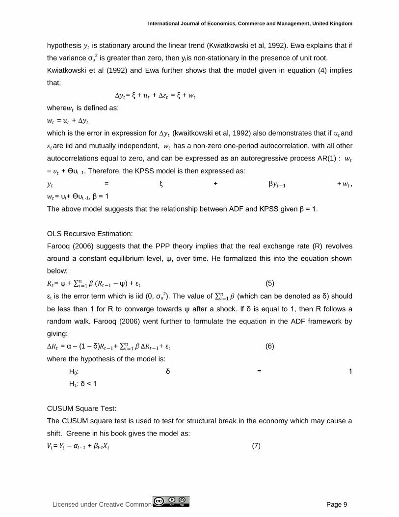
hypothesis 𝑦𝑡 is stationary around the linear trend (Kwiatkowski et al, 1992). Ewa explains that if

the variance ζu2 is greater than zero, then ytis non-stationary in the presence of unit root.

Kwiatkowski et al (1992) and Ewa further shows that the model given in equation (4) implies

that;

∆𝑦𝑡= ξ + 𝑢𝑡 + ∆휀𝑡 = ξ + 𝑤𝑡

where𝑤𝑡 is defined as:

𝑤𝑡 = 𝑢𝑡 + ∆𝑦𝑡

which is the error in expression for ∆𝑦𝑡 (kwaitkowski et al, 1992) also demonstrates that if 𝑢𝑡and

휀𝑡are iid and mutually independent, 𝑤𝑡 has a non-zero one-period autocorrelation, with all other

autocorrelations equal to zero, and can be expressed as an autoregressive process AR(1) : 𝑤𝑡

= 𝜐𝑡 + Өυt -1. Therefore, the KPSS model is then expressed as:

𝑦𝑡 = ξ + β𝑦𝑡−1 + 𝑤𝑡 ,

𝑤𝑡= υt+ ϴυt -1, β = 1

The above model suggests that the relationship between ADF and KPSS given β = 1.

OLS Recursive Estimation:

Farooq (2006) suggests that the PPP theory implies that the real exchange rate (R) revolves

around a constant equilibrium level, ψ, over time. He formalized this into the equation shown

below:

𝑅𝑡= ψ + 𝛽𝑛𝑖=1 (𝑅𝑡−1 – ψ) + εt (5)

εt is the error term which is iid (0, ζu2). The value of 𝛽𝑛

𝑖=1 (which can be denoted as δ) should

be less than 1 for R to converge towards ψ after a shock. If δ is equal to 1, then R follows a

random walk. Farooq (2006) went further to formulate the equation in the ADF framework by

giving:

∆𝑅𝑡 = α – (1 – δ)𝑅𝑡−1+ 𝛽𝑛𝑖=1 ∆𝑅𝑡−1+ εt (6)

where the hypothesis of the model is:

H0: δ = 1

H1: δ < 1

CUSUM Square Test:

The CUSUM square test is used to test for structural break in the economy which may cause a

shift. Greene in his book gives the model as:

𝑉𝑡= 𝑌𝑡 – αt - 1 + βt-1𝑋𝑡 (7)

© Karen


where αt – 1 and βt-1 denote the OLS estimates based on the first t-1 observations. Assuming ζst2

denotes the variance of the recursive residuals and 𝑤𝑡= 𝑣𝑡

σst and under the null hypothesis of no

structural change wt ~ N(0, ζ2). If the distribution of 𝑤𝑡changes over time, then there is a

structural change. CUSUM test is based on the cumulative sum of wt, and if the test statistics

are outside the confidence bound, then, the null hypothesis is rejected.

Chow Test:

This test was introduced by Gregory Chow in 1960 for the purpose of testing for structural

break. The model is shown as:

𝑦𝑡= a + b𝑥𝑡 + ε (8)

where the coefficients are assumed to change at t = t1, and are split into two groups; y1 and x1,

y2 and x2. The associated coefficients are B1 = a1, b1 and B2 = a2, b2. The null hypothesis is

then given as H0: B1 = B2.

In addition, the Chow test has an important limitation which is the break date which is made a

priori (Hansen, 2001). For this reason, researchers recommend the use of the Bai-Perron test

along with the chow test in order to test for accurate and correct results.

Bai-Perron Test:

The Bai-Perron test which has recently been developed by Bai J. and Perron P. in 2003 is used

to test for multiple structural breaks. Explaining that the problems of multiple structural changes

is not a lot but has an increasing attention. Considering a multiple linear regression, they show

the following model:

𝑦𝑡 = 𝑥𝑡ˊβ + 𝑧𝑡

ˊ + 𝑢𝑡 t = T j – 1 + 1,….,Tj (9)

for j = 1,…, m+1, 𝑦𝑡 is the dependent variable at time t; 𝑥𝑡 (p × 1) and 𝑧𝑡 (q × 1) are vectors of

covariates and β and 𝛿𝑗 (j = 1,..,m + 1) are the corresponding vectors of the coefficients; 𝑢𝑡 is

the error term at time t. The break points (𝑇1,…,𝑇𝑚 ) are treated as unknown. The unknown

regression coefficients together with the break points are estimated when observations at time T

are available. Furthermore, when p = 0, the pure structural change model is obtained, where all

the coefficients are subject to change and the breaks in the variance are permitted so long the

occur at the same dates as the breaks in the parameters of the regression (Bai and Perron,

2003).

As earlier stated, consumer prices and wholesale prices and effective nominal and real

exchange rate were estimated using the above tests. Testing for real exchange rate between

USA, Canada, Australia and Japan, to give an understanding of the variable used in the next



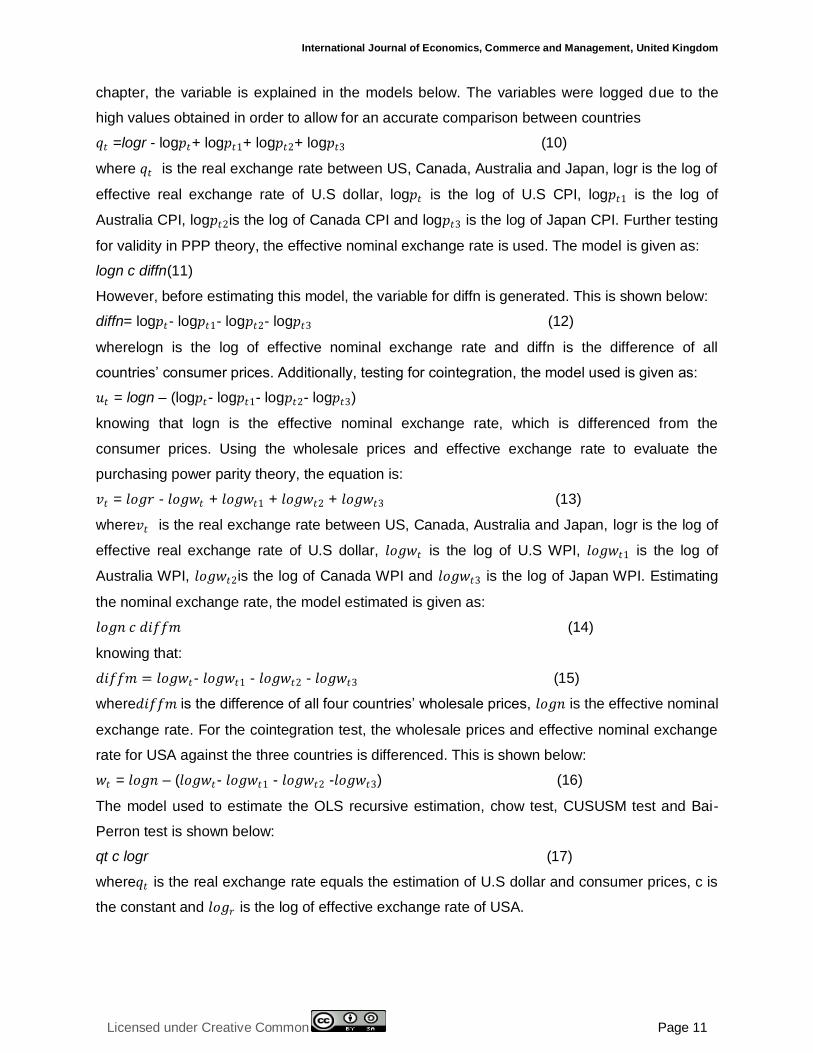
chapter, the variable is explained in the models below. The variables were logged due to the

high values obtained in order to allow for an accurate comparison between countries

𝑞𝑡 =logr - log𝑝𝑡+ log𝑝𝑡1+ log𝑝𝑡2+ log𝑝𝑡3 (10)

where 𝑞𝑡 is the real exchange rate between US, Canada, Australia and Japan, logr is the log of

effective real exchange rate of U.S dollar, log𝑝𝑡 is the log of U.S CPI, log𝑝𝑡1 is the log of

Australia CPI, log𝑝𝑡2is the log of Canada CPI and log𝑝𝑡3 is the log of Japan CPI. Further testing

for validity in PPP theory, the effective nominal exchange rate is used. The model is given as:

logn c diffn(11)

However, before estimating this model, the variable for diffn is generated. This is shown below:

diffn= log𝑝𝑡- log𝑝𝑡1- log𝑝𝑡2- log𝑝𝑡3 (12)

wherelogn is the log of effective nominal exchange rate and diffn is the difference of all

countries‟ consumer prices. Additionally, testing for cointegration, the model used is given as:

𝑢𝑡 = logn – (log𝑝𝑡- log𝑝𝑡1- log𝑝𝑡2- log𝑝𝑡3)

knowing that logn is the effective nominal exchange rate, which is differenced from the

consumer prices. Using the wholesale prices and effective exchange rate to evaluate the

purchasing power parity theory, the equation is:

𝑣𝑡 = 𝑙𝑜𝑔𝑟 - 𝑙𝑜𝑔𝑤𝑡 + 𝑙𝑜𝑔𝑤𝑡1 + 𝑙𝑜𝑔𝑤𝑡2 + 𝑙𝑜𝑔𝑤𝑡3 (13)

where𝑣𝑡 is the real exchange rate between US, Canada, Australia and Japan, logr is the log of

effective real exchange rate of U.S dollar, 𝑙𝑜𝑔𝑤𝑡 is the log of U.S WPI, 𝑙𝑜𝑔𝑤𝑡1 is the log of

Australia WPI, 𝑙𝑜𝑔𝑤𝑡2is the log of Canada WPI and 𝑙𝑜𝑔𝑤𝑡3 is the log of Japan WPI. Estimating

the nominal exchange rate, the model estimated is given as:

𝑙𝑜𝑔𝑛 𝑐 𝑑𝑖𝑓𝑓𝑚 (14)

knowing that:

𝑑𝑖𝑓𝑓𝑚 = 𝑙𝑜𝑔𝑤𝑡- 𝑙𝑜𝑔𝑤𝑡1 - 𝑙𝑜𝑔𝑤𝑡2 - 𝑙𝑜𝑔𝑤𝑡3 (15)

where𝑑𝑖𝑓𝑓𝑚 is the difference of all four countries‟ wholesale prices, 𝑙𝑜𝑔𝑛 is the effective nominal

exchange rate. For the cointegration test, the wholesale prices and effective nominal exchange

rate for USA against the three countries is differenced. This is shown below:

𝑤𝑡 = 𝑙𝑜𝑔𝑛 – (𝑙𝑜𝑔𝑤𝑡- 𝑙𝑜𝑔𝑤𝑡1 - 𝑙𝑜𝑔𝑤𝑡2 -𝑙𝑜𝑔𝑤𝑡3) (16)

The model used to estimate the OLS recursive estimation, chow test, CUSUSM test and Bai-

Perron test is shown below:

qt c logr (17)

where𝑞𝑡 is the real exchange rate equals the estimation of U.S dollar and consumer prices, c is

the constant and 𝑙𝑜𝑔𝑟 is the log of effective exchange rate of USA.

© Karen


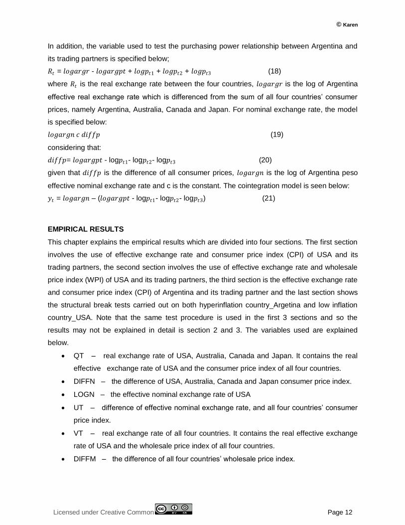
In addition, the variable used to test the purchasing power relationship between Argentina and

its trading partners is specified below;

𝑅𝑡 = 𝑙𝑜𝑔𝑎𝑟𝑔𝑟 - 𝑙𝑜𝑔𝑎𝑟𝑔𝑝𝑡 + 𝑙𝑜𝑔𝑝𝑡1 + 𝑙𝑜𝑔𝑝𝑡2 + 𝑙𝑜𝑔𝑝𝑡3 (18)

where 𝑅𝑡 is the real exchange rate between the four countries, 𝑙𝑜𝑔𝑎𝑟𝑔𝑟 is the log of Argentina

effective real exchange rate which is differenced from the sum of all four countries‟ consumer

prices, namely Argentina, Australia, Canada and Japan. For nominal exchange rate, the model

is specified below:

𝑙𝑜𝑔𝑎𝑟𝑔𝑛 𝑐 𝑑𝑖𝑓𝑓𝑝 (19)

considering that:

𝑑𝑖𝑓𝑓𝑝= 𝑙𝑜𝑔𝑎𝑟𝑔𝑝𝑡 - log𝑝𝑡1- log𝑝𝑡2- log𝑝𝑡3 (20)

given that 𝑑𝑖𝑓𝑓𝑝 is the difference of all consumer prices, 𝑙𝑜𝑔𝑎𝑟𝑔𝑛 is the log of Argentina peso

effective nominal exchange rate and c is the constant. The cointegration model is seen below:

𝑦𝑡 = 𝑙𝑜𝑔𝑎𝑟𝑔𝑛 – (𝑙𝑜𝑔𝑎𝑟𝑔𝑝𝑡 - log𝑝𝑡1- log𝑝𝑡2- log𝑝𝑡3) (21)

EMPIRICAL RESULTS

This chapter explains the empirical results which are divided into four sections. The first section

involves the use of effective exchange rate and consumer price index (CPI) of USA and its

trading partners, the second section involves the use of effective exchange rate and wholesale

price index (WPI) of USA and its trading partners, the third section is the effective exchange rate

and consumer price index (CPI) of Argentina and its trading partner and the last section shows

the structural break tests carried out on both hyperinflation country_Argetina and low inflation

country_USA. Note that the same test procedure is used in the first 3 sections and so the

results may not be explained in detail is section 2 and 3. The variables used are explained

below.

QT – real exchange rate of USA, Australia, Canada and Japan. It contains the real

effective exchange rate of USA and the consumer price index of all four countries.

DIFFN – the difference of USA, Australia, Canada and Japan consumer price index.

LOGN – the effective nominal exchange rate of USA

UT – difference of effective nominal exchange rate, and all four countries‟ consumer

price index.

VT – real exchange rate of all four countries. It contains the real effective exchange

rate of USA and the wholesale price index of all four countries.

DIFFM – the difference of all four countries‟ wholesale price index.



WT – difference of effective nominal exchange rate and all four countries‟ wholesale

price index.

RT – real exchange rate of Argentina, Australia, Canada and Japan which is computed

using effective real exchange rate, and CPI of all four countries.

DIFFP – the difference of Argentina, Australia, Canada and Japan.

LORGARN - Argentina effective nominal exchange rate.

YT – difference of Argentina effective nominal exchange rate and CPI of all four trading

partners.

These tests carried out is set to prove that PPP does not hold among these trading partners due

to failure to reject null hypothesis.

Section 1

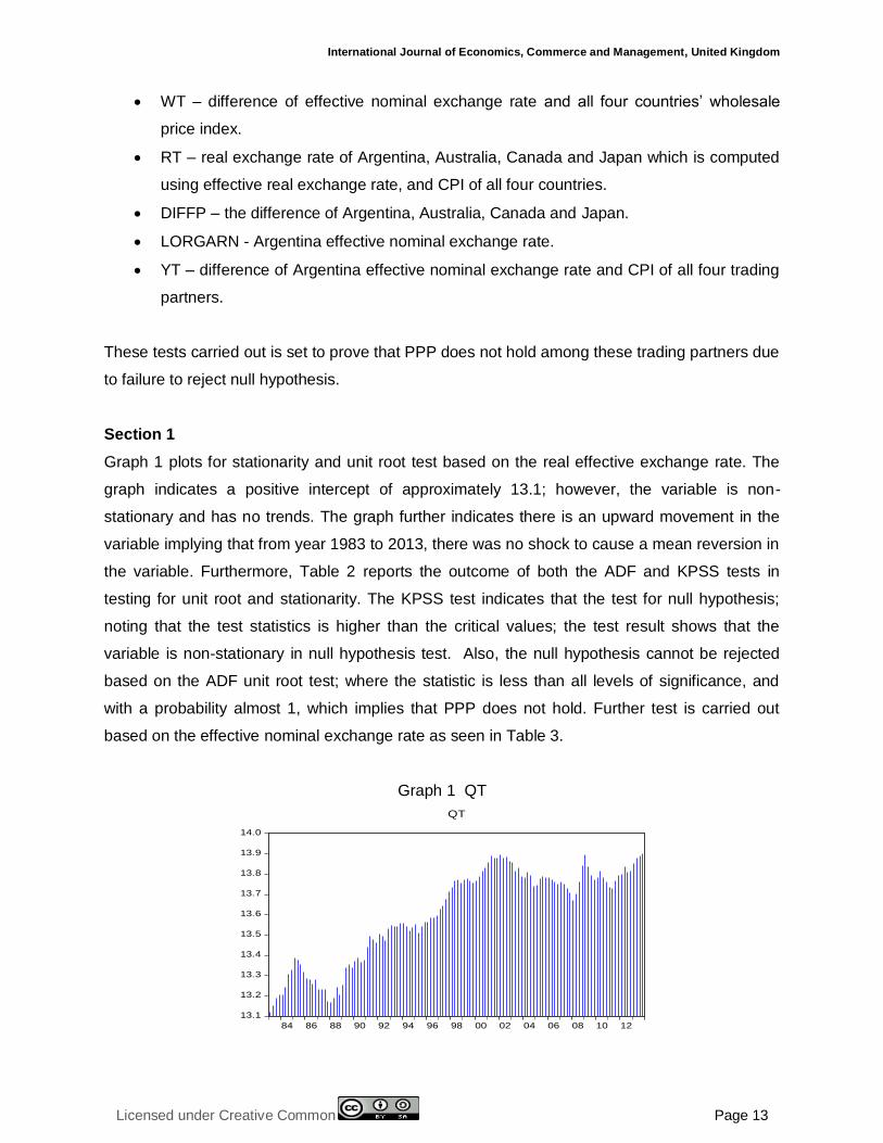
Graph 1 plots for stationarity and unit root test based on the real effective exchange rate. The

graph indicates a positive intercept of approximately 13.1; however, the variable is non-

stationary and has no trends. The graph further indicates there is an upward movement in the

variable implying that from year 1983 to 2013, there was no shock to cause a mean reversion in

the variable. Furthermore, Table 2 reports the outcome of both the ADF and KPSS tests in

testing for unit root and stationarity. The KPSS test indicates that the test for null hypothesis;

noting that the test statistics is higher than the critical values; the test result shows that the

variable is non-stationary in null hypothesis test. Also, the null hypothesis cannot be rejected

based on the ADF unit root test; where the statistic is less than all levels of significance, and

with a probability almost 1, which implies that PPP does not hold. Further test is carried out

based on the effective nominal exchange rate as seen in Table 3.

Graph 1 QT

13.1

13.2

13.3

13.4

13.5

13.6

13.7

13.8

13.9

14.0

84 86 88 90 92 94 96 98 00 02 04 06 08 10 12

QT

© Karen


Table 2 Unit Root and Stationarity Test

Augmented Dickey –Fuller Unit Root Test

Kwiatkowski-Phillips-Schmidt-Shin Test

.

Table 3 Test using Effective Nominal Exchange Rate

Variable Coefficient Probability

C -3.607734 0.0000

DIFFN -0.872779 0.0000

R-Squared 0.770762

F-statistic 410.1985

Probability (F-stat) 0.000000

Durbin-Watson Statistic 0.055712

Table 3 shows test of PPP employing nominal exchange rate. R2 0.77 which implies that the

total variability of the dependent variable is only explained by 77%. F-statistics indicates that the

variables are statistically significant with a p-value of 0.00. Durbin-Watson statistics been 0.05

leads to some doubts on the model which means the model suffers from positive serial

correlation. On the table, diffn is indicated to be negative, -0.87 which is far from 1. This result

therefore implies that PPP is not valid. Further estimation is carried out to verify the authenticity

of the above tests already done. Graph 2 tests for cointegration between effective nominal

exchange rate and the difference of CPI. The graphs show that the models are non-stationary

Null Hypothesis: QT is stationary

Exogenous: Constant, Linear Trend

LM-Stat.

Kwiatkowski-Phillips-Schmidt-Shin test statistic 0.250889

Asymptotic critical values*: 1% level 0.216

5% level 0.146

10% level 0.119



but there may be long run behaviour, which makes inference possible that PPP may hold in the

long run.

Graph 2 DIFFN & LOGN

Table 4 Unit Root Test for LOGN and DIFFN

I. Augmented Dickey –Fuller Unit Root Test

LOGN:


-9.6

-9.4

-9.2

-9.0

-8.8

-8.6

-8.4

84 86 88 90 92 94 96 98 00 02 04 06 08 10 12

DIFFN

3.6

3.8

4.0

4.2

4.4

4.6

4.8

84 86 88 90 92 94 96 98 00 02 04 06 08 10 12

LOGN

Null Hypothesis: LOGN has a unit root


t-Statistic Prob.*

Augmented Dickey-Fuller test statistic -1.172782 0.9111

Test critical values: 1% level -4.034997

5% level -3.447072

10% level -3.148578

Null Hypothesis: LOGN is stationary


LM-Stat.



5% level 0.146

10% level 0.119

© Karen


Table 4....

II. Augmented Dickey –Fuller Unit Root Test

DIFFN:


Drawing a conclusion from the cointegration test, residual series is generated and tested for

stationarity and unit root and null hypothesis is not rejected, indicating that PPP does not hold.

This is shown in Graph 3 and Table 5. The results report again, that null hypothesis is not

rejected and there is also no stationarity in null hypothesis test which corresponds with the test

above that PPP does not hold but may hold in the long run.

Graph 3 UT

Null Hypothesis: DIFFN has a unit root


t-Statistic Prob.*



5% level -3.447072

10% level -3.148578

Null Hypothesis: DIFFN is stationary


LM-Stat.



5% level 0.146

10% level 0.119

12.0

12.4

12.8

13.2

13.6

14.0

84 86 88 90 92 94 96 98 00 02 04 06 08 10 12

UT



Table 5 Unit Root and Stationarity Test UT



These tests carried out further implies that since there is inability to reject null hypothesis of

non-stationarity, then a conclusion is reached that PPP does not hold between the four

countries.

Section 2

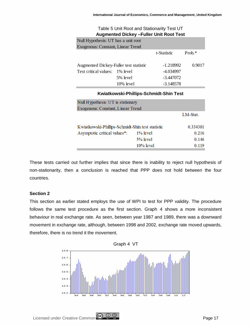
This section as earlier stated employs the use of WPI to test for PPP validity. The procedure

follows the same test procedure as the first section. Graph 4 shows a more inconsistent

behaviour in real exchange rate. As seen, between year 1987 and 1989, there was a downward

movement in exchange rate, although, between 1998 and 2002, exchange rate moved upwards,

therefore, there is no trend it the movement.

Graph 4 VT

Null Hypothesis: UT has a unit root


t-Statistic Prob.*



5% level -3.447072

10% level -3.148578

13.2

13.3

13.4

13.5

13.6

13.7

13.8

84 86 88 90 92 94 96 98 00 02 04 06 08 10 12

VT

© Karen


The graph shows a positive intercept beginning from 13.45, and there is also no shock of mean

reversion in the variable. The tests for stationarity and unit root test in table 6 infer that the null

hypothesis is non-stationary and is not rejected. The test in table 6 further shows that PPP does

not hold since null hypothesis cannot be rejected.

Table 6 Unit Root and Stationarity Test for VT



Using the nominal exchange rate, table 7 has an R2 0.55, this proposes that the total variability

of the dependent variable is only explained by 55%. F-statistics indicates that there is no

reversion and has a p-value of 0.00. Durbin-Watson statistics suffers from positive serial

correlation of been 0.04 leads to some doubts on the model which means the model suffers

from positive serial correlation.

Null Hypothesis: VT has a unit root


t-Statistic Prob.*



5% level -3.447072

10% level -3.148578

Null Hypothesis: VT is stationary


LM-Stat.



5% level 0.146

10% level 0.119





C -8.190032 0.0000

DIFFM -1.382361 0.0000

R-Squared 0.558134




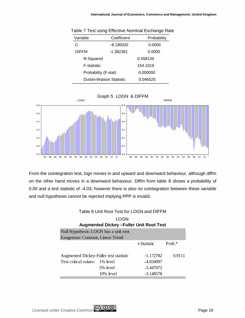
Graph 5 LOGN & DIFFM

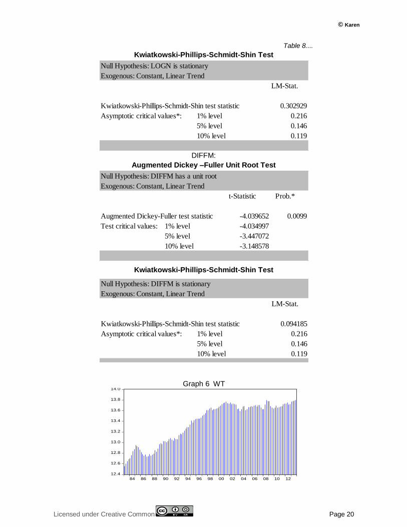
From the cointegration test, logn moves in and upward and downward behaviour, although diffm

on the other hand moves in a downward behaviour. Diffm from table 8 shows a probability of

0.00 and a test statistic of -4.03; however there is also no cointegration between these variable

and null hypothesis cannot be rejected implying PPP is invalid.

Table 8 Unit Root Test for LOGN and DIFFM

LOGN:


3.6

3.8

4.0

4.2

4.4

4.6

4.8

84 86 88 90 92 94 96 98 00 02 04 06 08 10 12

LOGN

-9.4

-9.3

-9.2

-9.1

-9.0

-8.9

-8.8

84 86 88 90 92 94 96 98 00 02 04 06 08 10 12

DIFFM

Null Hypothesis: LOGN has a unit root


t-Statistic Prob.*



5% level -3.447072

10% level -3.148578

© Karen


Table 8....


DIFFM:



Graph 6 WT

Null Hypothesis: LOGN is stationary


LM-Stat.



5% level 0.146

10% level 0.119

Null Hypothesis: DIFFM has a unit root


t-Statistic Prob.*



5% level -3.447072

10% level -3.148578

Null Hypothesis: DIFFM is stationary


LM-Stat.



5% level 0.146

10% level 0.119

12.4

12.6

12.8

13.0

13.2

13.4

13.6

13.8

14.0

84 86 88 90 92 94 96 98 00 02 04 06 08 10 12

WT



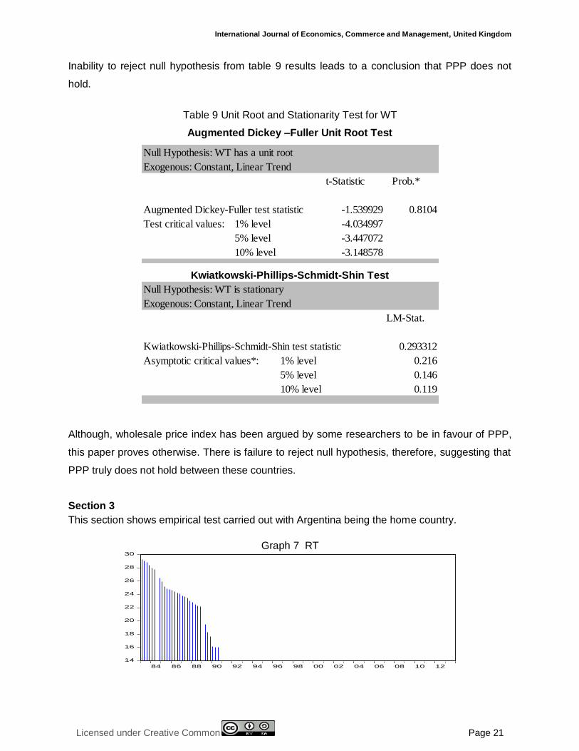
Inability to reject null hypothesis from table 9 results leads to a conclusion that PPP does not

hold.

Table 9 Unit Root and Stationarity Test for WT



Although, wholesale price index has been argued by some researchers to be in favour of PPP,

this paper proves otherwise. There is failure to reject null hypothesis, therefore, suggesting that

PPP truly does not hold between these countries.

Section 3

This section shows empirical test carried out with Argentina being the home country.

Graph 7 RT

Null Hypothesis: WT has a unit root


t-Statistic Prob.*



5% level -3.447072

10% level -3.148578

Null Hypothesis: WT is stationary


LM-Stat.



5% level 0.146

10% level 0.119

14

16

18

20

22

24

26

28

30

84 86 88 90 92 94 96 98 00 02 04 06 08 10 12

RT

© Karen


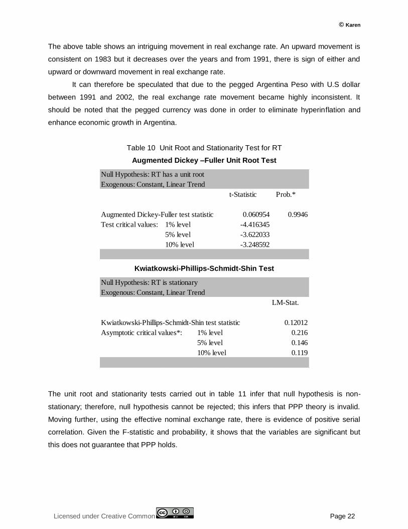
The above table shows an intriguing movement in real exchange rate. An upward movement is

consistent on 1983 but it decreases over the years and from 1991, there is sign of either and

upward or downward movement in real exchange rate.

It can therefore be speculated that due to the pegged Argentina Peso with U.S dollar

between 1991 and 2002, the real exchange rate movement became highly inconsistent. It

should be noted that the pegged currency was done in order to eliminate hyperinflation and

enhance economic growth in Argentina.

Table 10 Unit Root and Stationarity Test for RT



The unit root and stationarity tests carried out in table 11 infer that null hypothesis is non-

stationary; therefore, null hypothesis cannot be rejected; this infers that PPP theory is invalid.

Moving further, using the effective nominal exchange rate, there is evidence of positive serial

correlation. Given the F-statistic and probability, it shows that the variables are significant but

this does not guarantee that PPP holds.

Null Hypothesis: RT has a unit root


t-Statistic Prob.*

Augmented Dickey-Fuller test statistic 0.060954 0.9946


5% level -3.622033

10% level -3.248592

Null Hypothesis: RT is stationary


LM-Stat.



5% level 0.146

10% level 0.119





C -3.922432 0.0000

DIFFP -0.009726 0.0000

R-Squared 0.026154




Graph 8 shows that the variable are not cointegratedand from table 12, null hypothesis is not

rejected, therefore suggesting that PPP is invalid between Argentina and its trading partners.

Graph 8 LOGARGN & DIFFP

Table 12 LOGARGN:


2

4

6

8

10

12

14

16

84 86 88 90 92 94 96 98 00 02 04 06 08 10 12

LOGARGN

-26

-24

-22

-20

-18

-16

-14

-12

-10

84 86 88 90 92 94 96 98 00 02 04 06 08 10 12

DIFFP

Null Hypothesis: LOGARGN has a unit root


t-Statistic Prob.*



5% level -3.447072

10% level -3.148578

© Karen


Table 12.... Kwiatkowski-Phillips-Schmidt-Shin Test

DIFFP:



Graph 9 YT

Null Hypothesis: LOGARGN is stationary


LM-Stat.



5% level 0.146

10% level 0.119

Null Hypothesis: DIFFP has a unit root


t-Statistic Prob.*



5% level -3.447072

10% level -3.148578

Null Hypothesis: DIFFP is stationary


LM-Stat.



5% level 0.146

10% level 0.119

10

15

20

25

30

35

40

45

84 86 88 90 92 94 96 98 00 02 04 06 08 10 12

YT



Graph 9 and table 13 therefore suggest that PPP is not valid owing to the fact that null

hypothesis cannot be rejected.

Table 13 Augmented Dickey –Fuller Unit Root Test


Section 4

Further test is carried out on the USA and Argentina, testing for possible structural breaks over

time. As seen in graph 10, there is no stability over the years. There is a major structural change

in 1984 and 1985 and another structural change between 2002 to 2007.

Graph 10 Testing for possible structural breaks over time

Null Hypothesis: YT has a unit root


t-Statistic Prob.*



5% level -3.447072

10% level -3.148578

Null Hypothesis: YT is stationary


LM-Stat.



5% level 0.146

10% level 0.119

-4

0

4

8

12

16

20

84 86 88 90 92 94 96 98 00 02 04 06 08 10 12

Recursive C(1) Estimates

± 2 S.E.

© Karen


The possibility of structural break, that is, an unexpected shift at a point in time may lead to

some speculations. Graph 11 show that there is a structural break between 1990 and 1998,

where the test statistics is outside the confidence interval with 5% significance which implies

that the null hypothesis is rejected. Further test is carried out in Table 14 to verify the

authenticity of the CUSUM of squares test.

Graph 11 Testing for possible structural breaks over time (a)

Testing for the break point using the chow test, the time of financial crisis is used in order to

know if there was any structural break at a point in time and if this may have affected the

international trade. Result from table 13 does not authorize the acceptance of null hypothesis;

therefore, the null hypothesis is rejected, implying a structural break at that point in time.

Table 14 Chow Breakpoint Test: 2007 (Significance level: 5%)

Null Hypothesis: No breaks at the specified breakpoint

F-Statistics 14.53814 Probability F (2, 120) 0.0000

Log likelihood 26.90384 Probability Chi-Square (2) 0.0000

Wald Statistics 29.07629 Probability Chi-Square (2) 0.0000

Since null hypothesis has been rejected which the P-value is not significant at 5% interval, a

conclusion can be drawn that the structural break affected exchange rate and prices at that

time, therefore, playing a role in purchasing power parity. Table 15 further shows evidence of

multiple breakpoint and dates.

-0.2

0.0

0.2

0.4

0.6

0.8

1.0

1.2

84 86 88 90 92 94 96 98 00 02 04 06 08 10 12

CUSUM of Squares 5% Significance



Table 15 Multiple Breakpoints (Bai-Perron) Test for Real Exchange Rate

Tests F-statistics Critical Values Break Dates

5%

i = 1 270.52 11.47 1997

i = 2 103.06 12.95 1990

i = 3 24.65 14.03 2001

i = 4 13.68 14.85 2008

i = 5 0.00 15.29 -

Notes: The trimming weight is 0.15, which is used to calculate the statistics. The maximum

breakpoints are 5 and only 4 break points occurred.

As stated earlier that the structural break which occurred in 2007 due to financial crisis possibly

had an effect on exchange rate and prices. Bai-Perron test proves this by showing break dates.

The result shows that break dates that occurred were mainly in the 90‟s and 2000‟s. Having

carried out tests based on USA being a low-inflation country, the same test of recursive OLS

estimates and test for structural breaks is also carried out on Argentina being a high inflation

country.

Graph 12 shows an incoherent movement in the case of Argentina and there is evidence

of structural breaks over time ranging from 1985 to 1988 and again from mid-quarter of 1989 to

1990.

Graph 12 Incoherent movement

-40

-20

0

20

40

60

80

III IV I II IV I II III IV I II III IV I II III IV I II III IV II III IV I II III

1983 1984 1985 1986 1987 1988 1989 1990

Recursive C(1) Estimates

± 2 S.E.

© Karen


As stated earlier in the test carried out on Argentina, the presentation of test result may be due

to its pegging with USA and also the poor economy as at that time. The graph 13 below implies

that the test statistics is outside the confidence interval between years 1986 to 1990, meaning

that null hypothesis is rejected, implying a structural break; this was the period of poor economy

when Argentina peso had to be pegged to the U.S dollar.

Graph 13 CUSUM of Squares

Table 16 shows the breakpoint test in 1990 in which the Argentina peso was pegged to the U.S

dollar in order to reduce the national debt in Argentina. The result shows that there was indeed

a structural break considering that null hypothesis is rejected.

Table 16 Chow Breakpoint Test: 1990

Null Hypothesis: No breaks at the specified breakpoint

F-Statistics 15.59553 Probability F (2, 120) 0.0000

Log likelihood 23.48657 Probability Chi-Square (2) 0.0000

Wald Statistics 31.19105 Probability Chi-Square (2) 0.0000

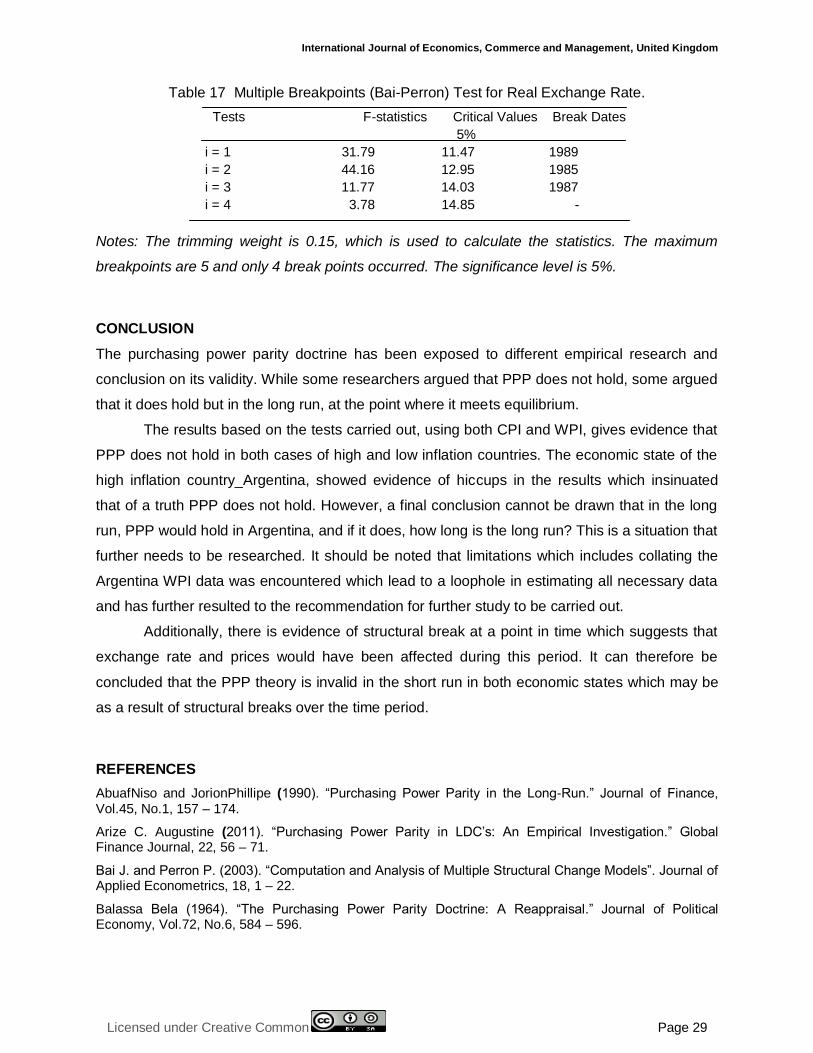
The test for possible structural breaks using the Bai-Perron tests shows the dates of structural

breaks. Although it does not specify the break date has shown in the chow test, but it still

reveals the structural changes from years before 1990.

-0.4

-0.2

0.0

0.2

0.4

0.6

0.8

1.0

1.2

1.4

III IV I II IV I II III IV I II III IV I II III IV I II III IV II III IV I II III

1983 1984 1985 1986 1987 1988 1989 1990

CUSUM of Squares 5% Significance



Table 17 Multiple Breakpoints (Bai-Perron) Test for Real Exchange Rate.

Tests F-statistics Critical Values Break Dates

5%

i = 1 31.79 11.47 1989

i = 2 44.16 12.95 1985

i = 3 11.77 14.03 1987

i = 4 3.78 14.85 -

Notes: The trimming weight is 0.15, which is used to calculate the statistics. The maximum

breakpoints are 5 and only 4 break points occurred. The significance level is 5%.

CONCLUSION

The purchasing power parity doctrine has been exposed to different empirical research and

conclusion on its validity. While some researchers argued that PPP does not hold, some argued

that it does hold but in the long run, at the point where it meets equilibrium.

The results based on the tests carried out, using both CPI and WPI, gives evidence that

PPP does not hold in both cases of high and low inflation countries. The economic state of the

high inflation country_Argentina, showed evidence of hiccups in the results which insinuated

that of a truth PPP does not hold. However, a final conclusion cannot be drawn that in the long

run, PPP would hold in Argentina, and if it does, how long is the long run? This is a situation that

further needs to be researched. It should be noted that limitations which includes collating the

Argentina WPI data was encountered which lead to a loophole in estimating all necessary data

and has further resulted to the recommendation for further study to be carried out.

Additionally, there is evidence of structural break at a point in time which suggests that

exchange rate and prices would have been affected during this period. It can therefore be

concluded that the PPP theory is invalid in the short run in both economic states which may be

as a result of structural breaks over the time period.

REFERENCES

AbuafNiso and JorionPhillipe (1990). “Purchasing Power Parity in the Long-Run.” Journal of Finance, Vol.45, No.1, 157 – 174.

Arize C. Augustine (2011). “Purchasing Power Parity in LDC‟s: An Empirical Investigation.” Global Finance Journal, 22, 56 – 71.

Bai J. and Perron P. (2003). “Computation and Analysis of Multiple Structural Change Models”. Journal of Applied Econometrics, 18, 1 – 22.

Balassa Bela (1964). “The Purchasing Power Parity Doctrine: A Reappraisal.” Journal of Political Economy, Vol.72, No.6, 584 – 596.

© Karen


Bahmani-Oskooee M. (1993). “Purchasing Power Parity based on Effective Exchange Rate and Cointegration: 25 LDC‟s experience with its Absolute Formulation.” World Development, Vol.21, No.6, 1023 – 1031.

Bahmani-Oskooee M. et al (2009). “Is PPP Sensitive to Time-Varying Trade in Constructing Real Effective Exchange Rate?” The Quarterly Review of Economics and Finance, Vol.49, 1001 – 1008.

Campos J. et al (1996). “Cointergration Tests in the Presence of Structural Breaks.” Journal of Econometrics, 70, 187 – 220.

Chen Y. and Rogoff K. (2002). “Commodity Currencies and Empirical Exchange Rate Puzzles.” DNB Staff Report, No.76

Corbae D. and Oularis D. (1988). “Cointegration and Tests of PPP” The Review of Economics and Statistics, Vol.70, No.3, 508 -511.

Dickey D. and Fuller (1979). “Distribution of the Estimators for Autoregressive Time Series with a Unit Root.” Journal of American Statistical Association, Vol.74, Issue 366, 427 – 431.

Edison J. Hali(1987). “Purchasing Power Parity in the Long-Run: A test of the Dollar/Pound Exchange Rate.” Journal of Money, Credit and Banking, Vol.19, No.3, pp. 376 – 387.

Ewa M. Syczewska.n.d.“Empirical Power of the Kwiastkowski-Philips-Schmidt-Shin Test” Warsaw School of Econometrics, Paper No. 3 – 10.

Farooq Q. Akram (2006). “Purchasing Power Parity in the Medium-Run: The Case of Norway.” Journal of Macroeconomics, 28, pp. 700 - 719.

Frenkel A. Jacob (1981). “The Collapse of Purchasing Power Parities during the 1970s‟.” European Economic Review, 16, 145 – 165.

Frenkel J. and Rose A. (1995). “A Panel Project on Purchasing Power Parity: Mean Reversion within and between Countries.” National Bureau of Economic Research, Working paper 5006.

Galliot J. Henry (1970). “Purchasing Power Parity as an Explanation of Long-term Changes in Exchange Rate.” Journal of Money, Credit and Banking, Vol.2, No.3, pp. 348 – 357.

Glen D. Jack (1992). “Real Exchange Rates in the Short, Medium and Long-run.” Journal of International Economics, 33, pp. 147 – 166.

Greene H. William (2012). “Econometric Analysis”. 7thEd. Essex: Pearson.

Hakkio S. Craig (1982). “A Re-examination of Purchasing Power Parity: A Multi-country and Multi-Period study.” National Bureau of Economic Research, No. 865.

Hensen E. Bruce (2001). “The New Econometrics of Structural Change: Dating Breaks in U.S Labour Productivity.” Journal of Economics Perspective, Vol.15, Bo.4, 117 – 128.

Kim Yoonbai (1990). “Purchasing Power Parity in the long run: A Cointegration Approach.” Journal of Money, Credit and Banking, Vol.22, No.4, pp. 491 – 503.

Kwiatkowski D. et al (1992). “Testing the null hypothesis of stationarity against the alternative of a unit root.” Journal of Econometrics, 54, pp. 159 – 178.

Officer Lawrence (1980). “Effective Exchange Rate and Price Ratios over the long run: A test of the Purchasing Power Parity Theory.” The Canadian Journal of Economics, vol.13, No.2.

Pakkio R. Michael and Pollard S. Patricia (2003). “Burgernomics: The Big Mac Guide to Purchasing Power Parity” Federal Reserve Bank of St. Louis Review,85, 6, pp. 9 – 28.

Rogoff Kenneth (1996). “The Purchasing Power Parity Puzzle.” Journal of Economic Literature, Vol.34, No.2, pp.647 – 668.

Sabate M. et al (2003). “PPP and Structral Breaks: The Peseta-Sterling Rate, 50yearsa of a floating regime” Journal of International Money and Finance, 22, 613 – 627.

Taylor M. Alan and Taylor P. Mark (2004). “Purchasing Power Parity Debate.” Journal of Economics Perspectives, Vol.18, No.4, pp. 135 – 158.



Yin-Wong Cheung and Kon S. Lai. (1993). “A Fractional Cointergration Analysis of Purchasing Power Parity.” Journal of Business and Economic Statistic, Vol. 11, No.1.

Yin-Wong Cheung and Kon S. Lai. (1994). “Mean Reversion in Real Exchange Rates.” Economic Letters, 46, pp. 251 – 256.

EVALUATING PURCHASING POWER PARITY IN ... - …ijecm.co.uk/wp-content/uploads/2015/01/311.pdf ·...

Documents

Transcript of EVALUATING PURCHASING POWER PARITY IN ... - …ijecm.co.uk/wp-content/uploads/2015/01/311.pdf ·...