Evaluating of the Impact of Conditional Cash Transfers on Schooling:

An Experimental Analysis of Honduras’ PRAF Program

Paul Glewwe (University of Minnesota)

Pedro Olinto (IFPRI-FCND)

Final Report for USAID

January, 2004

Abstract

This report assesses the impact of the education interventions of the PRAF II program on educational outcomes of children age 6-13 in rural areas of Honduras. Two interventions were examined, a “demand” intervention that provided families with monetary payments if their children were enrolled in (and regularly attended) primary school, and a supply side incentive that provided assistance to schools. Econometric estimates suggest that the demand side intervention of the PRAF II program increased enrollment rates by 1-2 percentage points, reduced the dropout rate by 2-3 percentage points, increased school attendance (conditional on enrollment) by about 0.8 days per month, and increased annual promotion rates to the next grade by 2-4 percentage points. There was no effect on child labor force participation. Some of these impacts appear to be negatively correlated with household income, which implies that they are stronger for poorer households. Simulation results indicate that, over the long run, the demand intervention will increase the years of schooling of 14 year old children by about 0.7 years. In contrast, the supply side intervention has had no effect on any outcomes, which is not surprising given that most parts of it were never implemented.

1

I. Introduction

The Programa de Asignacion Familiar (PRAF) is one of the largest government

social welfare programs in Honduras, the third poorest country in Latin America and the

Caribbean (in terms of per capita GNP). PRAF was initiated in 1990 as a social safety

net to compensate the poor for lost purchasing power brought about by macroeconomic

adjustment. It was restructured in 1998, and now includes a reformulated project known

as PRAF/IDB - Phase II (henceforth referred to as PRAF II). The objective of this project

is to encourage poor households to invest in their family's education and health by

providing incentives to increase primary school enrollment, the use of preventive health

care services, and the quality of both education and health-care services.

An unusual and important feature of the PRAF II project is that it includes a

monitoring and evaluation component managed by the International Food Policy

Research Institute (IFPRI) to assess the program’s impact over time. In particular,

among a set of 70 poor rural communities in Honduras, PRAF II was implemented in

some but not others, as determined by random assignment. This paper uses this random

assignment to evaluate the impact of PRAF II on education outcomes on poor rural

communities in Honduras.

This paper is organized as follows. The next section explains the PRAF program

and the data that have been collected for evaluating it. Section III provides some

descriptive statistics from data collected in 2000, just before the launching of the

program. An analysis of the impact of program on several education outcomes, including

enrollment, attendance and grade repetition, is presented in Section IV. Finally, Section

V summarizes the findings and provides some brief concluding remarks.

2

II. Description of PRAF II and the Data Available to Evaluate It

Honduras's Family Allowances Program (PRAF) began operation in 1990. The

program was initially intended to be a temporary program to ease the burden of

macroeconomic adjustment on poor households. PRAF was originally a cash transfer

program, distributing cash grants from health centers and schools. Continued widespread

poverty in Honduras extended the time horizon of PRAF beyond the initial

macroeconomic adjustment period. In addition, the objective of the program was

changed; instead of only alleviating poverty it was now given the task of eradicating the

root causes of poverty. The root causes were seen as lack of human capital among poor

families, so the program was modified to provide assistance that would enable those

families to increase their human capital, particularly the health and education of children

in poor families.

A. The PRAF II Program

In 1998, the Honduran government modified PRAF to redirect it toward these

new objectives. This modified program will be referred to as PRAF II in the rest of this

paper. PRAF II has the following specific objectives: (i) boost the demand for education

services; (ii) encourage the “education community” to take part in children's learning

development; (iii) instruct mothers of young children in feeding and hygiene practices;

(iv) ensure that sufficient money is available for a proper diet; (v) promote demand for,

and access to, health services for pregnant women, nursing mothers and children under

age 3; and (vi) ensure timely and suitable health care for PRAF beneficiaries. More

3

generally, the objective of PRAF II is to increase the health and education of Honduran

children in poor rural communities.

PRAF II has the following distinctive features: (i) a new system for selecting

beneficiaries; (ii) interventions to stimulate the demand for and the supply of education,

nutrition and health services; (iii) baseline data collection and subsequent annual data

collection to measure outcomes and progress under the program; (iv) assessment of the

program based on randomized treatment and control groups. PRAF II is being piloted in

70 of the poorest municipalities in Honduras. The municipalities were selected in

October, 1999, and the interventions begain in late 2000.

To estimate the impacts of both the supply side and the demand side

interventions, IFPRI designed an evaluation procedure in which the 70 municipalities

were assigned randomly to four different groups, designated as G1 – G4:

G1 = Demand side intervention only (20 municipalities)

G2 = Demand and supply side interventions (20 municipalities)

G3 = Supply side intervention only (10 municipalities)

G4 = Control group without intervention (20 municipalities).

This design allows for measurement of the impact of the demand side interventions, the

supply side interventions, and of both interventions.

In each municipality in groups G1-G3, both health and education projects are

implemented. For both health and education, interventions take two distinct forms: a)

demand side incentives (cash transfers) conditioned on school attendance and/or frequent

heath clinic visits by the recipient; and b) supply side investments, aimed at improving

the quality of schooling and health services supplied in poor rural areas. The demand

4

side intervention for health consists of monetary transfers to pregnant women and to

mothers of children under three years of age. The voucher is provided only for women

who have visited health clinics every month as required by the program. Each family

may receive up to twohree vouchers per month (one woman and one child, or up to two

children), each worth approximately US$4.

The supply side intervention for health consists of monetary transfers to

primary health care teams, which are formed by members of the community and local

health care workers (nurses and, when available, doctors). To receive the transfers, each

team must prepare a plan with specific tasks and a budget specifying what equipment and

medicine will be purchased for the health center. Each team receives, on average,

US$6,000 per year; but the amount varies from US$3,000 to US$15,000, depending on

the size of the population served by the health center.

The demand side incentive for education is generated using monetary payments

to families for each child age 6-12 who is enrolled in the first four years of primary

school and attends regularly. A maximum of up to three children per family are eligible

(this is in addition to any monetary payments received from the demand side incentives

from the health intervention). The family receives approximately US$5 per month for

each eligible child. To be eligible for a payment, the child needs to be enrolled by the

end of March (the school year in Honduras begins in March and ends in December) and

to maintain an attendance rate of 85%. In fact, although the enrollment requirement was

strictly enforced there were serious problems monitoring attendance, so that for most

families the 85% attendance requirement was not enforced.

5

The supply side education intervention consists of payments to the Parent

Teacher Associations (PTAs) associated with each primary school. Theses associations

were required to obtain legal status and to prepare plans to improve the quality of the

education provided by their respective schools. A plan was required to include a budget

for the educational materials and equipment (selected from a menu of items approved by

PRAF II) needed for the plan. On average, the schools were eligible to receive US$4,000

per year; the actual figures ranged from US$1,600 to US$23,000, depending on the size

of the school (for details on the calculation of the exact amounts, see UCP/IFPRI, 2000).

B. Data

After the 70 poor municipalities were chosen, baseline data were collected from

all 70 before the PRAF II program was implemented in the municipalities in groups G1,

G2 and G3. The baseline data were collected in 2000, from mid-August to mid-

December September. The follow-up survey was conducted approximately two years

later, from mid-May to mid-August of 2002. From each of the 70 municipalities, eight

communities (“clusters”) were randomly selected, and from each cluster 10 dwellings

were randomly selected (see IFPRI, 2000, for details of the sampling methodology).

Assuming one household per dwelling, this implies a total sample of 5600 households. In

fact, some of these dwellings had more than one household, so the total number of

households selected was 5748. In most cases, each group of 10 dwellings is found within

a different village (aldea) of the municipality, but in some cases two or more groups of 10

are from the same village. These 5748 households contained a total of 30,588 members.

Three kinds of data were collected in 2000. First, the household questionnaire

collected data on: a) housing; education and employment of all household members; b)

6

education (very detailed) of all children age 6-16; c) the health of all women who were

pregnant in the past 12 months; d) the health of all children below three years of age (and

height, weight and hemoglobin information for all children under five years); e)

consumption expenditures on food and non-food items; f) access to credit; g) remittances

received from household members who have moved away; h) receipt of assistance from

various government and private agencies (including from PRAF); i) ownership of

livestock and durable goods; j) time spent by the “woman of the house” and by children

age 6-12 doing various activities; and k) households’ evaluation of the quality of local

health centers and primary schools.

Second, data were collected on community characteristics in each of the 560

clusters. The data include: a) whether the community has a primary school, a public

hospital or public transport; b) daily wage rates for local agricultural and non-agricultural

work; c) the availability of work away from the community; d) a small amount of

information on local crime; and e) prices for a large number of food items and local daily

wages rates.

Third, questionnaires were administered to primary schools in each of the 70

municipalities. Three schools were randomly selected from each municipality. The

school questionnaire collected the following data: a) general information on the school

(days open, number of grades, etc.); b) characteristics of teachers; c) pedagogical aids

(library books, dictionaries, paper etc.); and d) school organizations (PTA, teachers

association, etc.).

In the 2002 follow-up survey, about 92% of the 5748 households in the 2000

survey were reinterviewed. This high reinterview rate reflects attempts made to follow

7

households that moved. (More specifically, all children aged 0-13 years and all woman

aged 15-49 who still lived in one of the seven departments from which the 70

municipalities were drawn were targeted to be followed in 2002). In addition, household

members who left the households they belonged to in 2000, either to from a new

household or to join an existing household, were followed if they were part of PRAF II’s

target population: pregnant women, lactating mothers, and children age 0-16 years.

Table 1 provides detailed information about the sample of children used in the

analysis of this paper. Children who had the opportunity to participate in the program at

some point between late 2000 and late 2002 were those born between March 2, 1988 and

March 1, 1996. (Any child born on or before March 1, 1988, would have been 13 years

old or older at the start of the school year in March 1, 2001, and thus would not be

eligible to participate in the program, and any child born March 2, 1996 or later would

have been age 5 or younger at the start of the school year in March 1, 2002, and thus

would be too young to participate in the program.) In the baseline survey conducted in

2000, there were 7678 children in this age range in the full sample (all 70 municipalities).

Of these children, 4.9% (376) were gone from the sample by the time of the follow-up

survey conducted in 2002 because the household that they had belonged to was not

reinterviewed. The three main reasons that a household was not reinterviewed, in order

of importance, were that the dwelling could not be found (which accounts for 169 of the

376 children in such households), the household was absent from the dwelling (100 of the

376 children) and that the household refused to be interviewed (57 children). Finally,

some of the children in the households that were reinterviewed in 2002 were not

reinterviewed, which led to an additional loss of 3.3% (250 children) of the original

8

sample of children. The main reason for this is that children moved away from the

household and could not be followed up to be reinterviewed.

This sample attrition implies that 91.8% (7052) of the original 7678 children were

reinterviewed in the 2002 follow-up survey. This attrition rate is not particularly large

and as such it should not have a large impact on the estimates presented below. Even

more importantly, the attrition rate is similar for all four groups, the three in which an

intervention was implemented on the one that served as a control group. Specifically, the

retention rates for the four groups were 92.7% for G1, 92.1% for G2, 92.0% for G3 and

90.7% for G4. Thus the control group had a retention rate that was only slightly lower

than those of the other groups. The main difference appears to be in the higher refusal

rate, which may reflect a small number of households in the control group were

disappointed as being in a group that did not receive any program benefits.

A final aspect of the data collection, which will have implications for interpreting

the results in Section V, concerns the timing of the interviews across the four groups of

municipalities. As seen in Table 2, there is little correlation between the month of

interview and group assignment in 2002, but there is a strong correlation in 2000. In

particular, the interviews in 2000 were conducted for the demand only (G1) and supply

and demand (G2) interventions in August, September and October, while those for the

supply only (G3) and the control group (G4) were conducted in November and

December. While this difference in time may not appear to be very large, there is an

important factor at work, which is that November and December are important months

for harvesting coffee in Honduras, and many of the households in the sample, including

many relatively young children, are engaged in this work. This implies that differences

9

in school attendance and in labor force participation in 2000 across the four groups of

municipalities could appear to be quite different simply because the dates of interview

were different for the different groups. This issue will be discussed in more detail in

Section V.

III. Education Outcomes from the 2000 Baseline Data

Before examining the impact of the PRAF II program on education outcomes, it is

useful to establish a context for the analysis by presenting some basic data on the

education outcomes of children of primary school age in 2000 (before the program was

implemented).

Table 3 shows the ages at which children of different ages started primary school.

Although the official policy of Honduras’ Ministry of Education is that children should

begin school at age 76, [or, children have to start school in the year that they turn 7] only

21% of 6-year-old children from these 70 poor municipalities have started schooling.

Part of this low enrollment rate is due to the fact that many of the children who were six

years old at the time of the survey (interviews were conducted in August through

December) could have been five years old when school started in March, but the fact that

28% of children who are seven years old at the time of the survey had not yet started

primary school indicates that delayed enrollment is common in these rural areas of

Honduras. By age 10, 95% of these children have started primary school, and this

percentage peaks at about 96% at age 12. Thus at most only about 4% of the children in

these poor municipalities never attend school, but delayed enrollment in primary is a

10

common phenomenon. The table also provides these figures by sex; girls are slightly

more likely to start on time, but the difference is not very large.

Table 4 shows enrollment in 2000 for all children from ages 6-16. The older

children are included to show the ages at which children drop out. For all children in

these 70 municipalities, enrollment peaks at 86-87% at ages 8-10, after which it steadily

declines so that only about 15% of 16-year-olds are enrolled in school. (Note that ages 6

and 7 include some children who are still enrolled in pre-school.) Even by age 13 only

about half of these children are still enrolled in school. Girls are more likely to be

enrolled in school at all ages, but the difference is not very large.

The tables examined so far show that almost all (96%) of Hondurans children in

these poor municipalities eventually do enroll in primary school, yet they often start their

schooling 1-2 years late and they do not stay in school very long. In particular, about half

have dropped out by age 13 and about 85% have dropped out by age 16. This implies

that these children complete only a few years of schooling before leaving school. This is

shown in Table 5, which shows years of schooling completed for children who are 16

years old (at the time of the survey). About 15% have not completed a single year of

primary school, and about one fourth completed only 1-3 years of schooling. A common

rule of thumb is that four or more years of schooling are needed before someone acquires

and retains basic literacy skills, which implies that about 40% of the children in these

communities will be illiterate when they become adults. About half (48%) attain 4-6

years of schooling, and only 12% attain seven or more years (i.e. secondary school).

Clearly, school attainment in these Honduran communities is quite low and fully justifies

programs to increase it.

11

The next three tables examine patterns that may explain why children are not

enrolled in school. Table 6 examines whether children from age 6 to 16 have started

primary school and whether they are currently enrolled in school, by income levels.

More precisely, children were divided into four groups of equal size according to

household consumption expenditures per capita. The poorest 25% are called quartile 1,

the next poorest 25% are quartile 2, and so on. For the poorest quartile, only 79% have

started primary school and only 55% are currently enrolled in school. These numbers

increase steadily for wealthier groups, until at the fourth quartile (wealthiest 25%) 89% of

these children have started primary school and 74% are still in school. This suggests, as

one would expect, that better off households are more likely to enroll their children in

school.

Another factor which could have a strong impact on children’s schooling

outcomes is their parents’ level of education, especially mothers’ education. Table 7

looks at starting primary school and current school attendance when children are

classified according to their mothers’ level of education. About one third (36%) of

children age 6-16 have mothers with no education at all. About 80% of those children

had started primary school, and only 57% were currently attending school. Children

whose mothers had some primary school education (1-5 years) fared better; 85% had

started primary school and 65% were currently attending school. Children whose

mothers had completed primary schooling (about 12% of the sample) performed best of

all, with 87% starting primary school and 82% currently in school. Somewhat

surprisingly, the small number of children whose mothers report higher than primary

education (0.4% of the sample) did not do as well as mothers who had some or complete

12

primary education; this could reflect the small sample size or it may simple indicate that

these women were misclassified.

Another potentially important determinant of school progress is the distance to the

nearest primary school. All households were asked how long it would take them to walk

to the primary school that is nearest to their homes. Two thirds (68%) of the children live

in households where this travel time (one way) is 15 minutes or less. About one fourth

(23%) live in households were the travel time is 16-30 minutes, while another 6% have

travel times of 31-60 minutes and 2% report travel times of more than one hour (the

largest was five hours). Table 6 examines the relationship between travel time, starting

primary school and current school attendance. About 85% of children who live within 15

minutes of a primary school have started primary school. This figures drops to 82% for

children with travel times of 16-30 minutes and 74% for children with times of 31-60

minutes, and then increases slightly to 78% for children with times exceeding one hour.

Current school enrollment has a clear monotonic relationship, ranging from 66% for

children within 15 minutes of a primary school to 43% for children whose travel times

exceed one hour.

IV. Empirical Methods: Estimating the Impact of PRAF II on Education Outcomes

The central problem in the evaluation of any social program is that fact that

households who have the opportunity to benefit from the program cannot be observed

simultaneously in the state of participating in the program and the state of not

participating in the program. That is, for a household that participates one does not

observe what the situation would have been had the household not participated, and for a

13

household that does not participate one does not observed what would have occurred had

that household participated.

A. The Main Parameter to Be Estimated, and Two Estimation Strategies

To state the above point more formally, let Y1i be the outcome of interest for

individual (or household) i if he or she were to participate in the program being

evaluated, and let Y0i be the outcome of interest if he or she were not to participate. The

impact of participating in the program for individual i can then be defined as ∆i = Y1i –

Y0i. The problem is that for any individual i one observes only Y1i (if he or she

participates) or only Y0oi (if he or she does not participate), which implies that for all

individuals one cannot calculate ∆i unless one makes some additional assumptions. The

following paragraphs explain two methods for overcoming this problem; for a much more

general and detailed discussion, see Heckman, Lalonde and Smith (1999).

This paper follows the vast majority of papers in the program evaluation literature

in that it is primarily concerned with estimating average program impacts, as opposed to

estimating impacts for individual persons or households in the data. That is, the main

question addressed is the impact of the program on the mean value of an outcome of

interest. More specifically, for this evaluation of PRAF II the main objective is to

estimate a single parameter: the mean (direct) effect of offering the opportunity to

participate in the program (offering the “treatment”). The only exception to this is that

some estimates add a term that shows how the program effect varies by household

income levels; this is explained in more detail below.

Not only is the main parameter of interest defined in terms of mean effects, but

note also that all estimates measure the effect of offering the treatment (offering the

14

opportunity to participate in the program), not the mean effect of the treatment on the

treated (mean effect of the program on those who choose to participate). These two

effects differ because some people who are offered the possibility of participating in a

program choose not participate. When this occurs, there is likely to be a difference

between the impact on Y of the opportunity to participate in the program and the impact

on Y for individuals or households that choose to participate in the program. The latter,

by definition, is defined not for the population as a whole but only for those members

who choose to participate. Of course, if every person or household that is offered the

opportunity to participate in the program chooses to do so, then these two impacts are

identical. But if some choose not to participate then they are different, and some

households that had the opportunity to participate in PRAF II in fact chose not to do so

(as will be seen in Section V).

The data at hand for evaluating PRAF II are well suited for estimating the mean

impact of offering the treatment (offering the opportunity to participate in the PRAF II

program), as will be seen below, but they are not well suited for estimating the mean

impact of the treatment on the treated. The reason for this is that the type of

randomization done under PRAF II does not allow one to know which individuals in the

control group (the group not offered the opportunity to participate in the program) would

have participated had they had the opportunity to do so. Thus it is not possible to observe

Y for a group of persons who did not participate in PRAF II because they were not

offered the opportunity to do so (i.e. they were in the control group) and would have

participated if they had been given the opportunity.

15

Returning to the parameter that can be estimated, the mean effect on Y of being

offered the opportunity to participate in PRAF II can be defined formally using the

expectations operator E[ ] as:

E[YOff – Y0| O = 1, X] = E[YOff| O = 1, X] - E[Y0| O = 1, X] (1)

where O = 1 signifies the offer to participate in the program, YOff is the value of Y after a

person responds to the offer to participate (choosing either to participate or not to

participate), and X is a set of variables that can be used to define population subgroups of

particular interest. It is important to note that YOff is not necessarily equal to Y1;

although YOff = Y1 for those to choose to participate, YOff = Y0 for those who choose not

to participate. Thus the expression in equation (1) is not equal to E[Y1 – Y0| O = 1, X] =

E[∆| O = 1, X].

In any population it is relatively simple to collect data that can be used to estimate

E[YOff| O = 1, X], the value of Y for all people who had the opportunity to participate in

the program. The difficulty is in estimating E[Y0| O = 1, X], the value of Y that would be

observed if the people who were offered the opportunity to participate had not had that

offer. The problem is that many people take up the offer, so what would have occurred

had no offer been available is not observed. This paper uses the randomized design of

the PRAF II program to obtain two different estimates of E[Y0| O = 1, X], which are then

combined with the more easily estimated E[YOff| O = 1, X] to estimate of E[YOff – Y0| O

= 1, X]. The first is called the cross-sectional difference estimator, which will be denoted

16

as CSDIF, and the second is called the double difference (or difference in differences)

estimator, which will be denoted as 2DIF.

The intuition behind the CSDIF estimator is very simple. Although one cannot

observe Y0 for the entire population of those who were offered the opportunity to

participate in the program (since many of them took up the offer and thus one observes

Y1 instead of Y0), if there is another group that is not systematically different in any way

from the group that was offered the opportunity to participate, and that group was not

offered the opportunity to participate, then the values of Y for that group, which can be

denoted as E[Y0| O = 0, X] (O = 0 indicates that this group was not offered the

opportunity to participate) should be an unbiased estimate of E[Y0| O = 1, X]. This

implies that the CSDIF estimator can be defined as:

CSDIF ≡ E[YOff| O = 1, X] - E[Y0| O = 0, X] (2)

= E[Yt| O = 1, X] - E[Yt| O = 0, X] t = 1, 2, …

The second line of equation (2) simply indicates that Y is measured at the same time for

both the group that was offered the opportunity to participate in the program (O = 1) and

the group that was not offered the opportunity to participate (O = 0), where any t ≥ 1 is a

time period after the program has been implemented for the group that has been offered

the opportunity to participate. Since the group for which O = 1 has had the opportunity

to participate in the time periods t = 1, 2,… etc., then YOff = Yt for all individuals who

were offered the opportunity to participate (O = 1). Similarly, Y0 = Yt for the time

periods t = 1, 2,… for all individuals who were not offered the opportunity to participate

17

(O = 0). This notation in the second line also clarifies why this estimator is called the

cross-sectional difference estimator – it can be estimated using data collected at one point

in time for any t ≥ 1 as long as there is a “control group” available for estimating

E[Yt| O = 0, X].

The 2DIF estimator can be interpreted as a cross-sectional estimator that has a

“correction factor” added that accounts for the possibility that Y0 differed between the

two groups (the group offered the opportunity to participate in the program and the group

not offered the opportunity to participate) before the program was implemented. Such

differences could be due simply to random chance or to some error in the implementation

of the randomization scheme. Whether any such difference is large can also be checked,

as discussed below. The correction factor is E[Yt=0| O = 1, X] - E[Yt=0| O = 0, X], the

difference in Y fror the two groups before the program was available to either group.

Subtracting this factor from the CSDIF estimator yields:

2DIF = E[Yt| O = 1, X] - E[Yt| O = 0, X] – {E[Yt=0| O = 1, X] - E[Yt=0| O = 0, X]} (3)

= {E[Yt| O = 1, X] - E[Yt=0| O = 1, X]} – {E[Yt| O = 0, X] - E[Yt=0| O = 0, X]} t = 1, 2, …

The second line of equation (3) shows why this is referred to as the double difference

estimator; for both groups the difference is calculated in Y before and after the program,

and then these two terms are differenced.

One final point to note is that if there were no problems in randomizing the

treatment, there should be no difference between E[Yt=0| O = 1, X] and E[Yt=0| O = 0, X].

That is, E[Yt=0| O = 1, X] - E[Yt=0| O = 0, X] = 0, which implies that CSDIF = 2DIF.

18

B. Implementing the Estimation Strategies within a Regression Framework

Standard multiple regression methods can be used to estimate the impact on Y of

being offered the opportunity to participate in the program using either the CSDIF

approach or the 2DIF approach. To see how this works, consider the following

regression equation:

Yit = α + βOOi + βtti + βO,tOiti + Σ=

J

0jθjXj + εit, t = 0, 1, 2, … (4)

In this regression, Yit is the value of Y for person i at time t, Oi is a dummy variable that

equals 1 if person i is offered the opportunity to participate in the program and 0 if he or

she is not offered the opportunity to participate, ti is a dummy variable that equals zero if

the time period is 0 (the time period before the program was implemented in the first

group) and equals one if the time period is ≥ 1 (some time period after the program was

implemented), Xj is one of several control variables, and εit is a random error term that is

assumed to be uncorrelated with the observed variables. If the opportunity to participate

in the program was in fact randomly assigned, then εit will be uncorrelated with Oi.

Given estimates of the regression parameters in equation (4), the components that

are used to estimate CSDIF and 2DIF are:

E[Yt=0| O = 0, X] = α + Σ=

J

0jθjXj (5a)

E[Yt=0| O = 1, X] = α + βO + Σ=

J

0jθjXj (5b)

19

E[Yt≥1| O = 0, X] = α + βt + Σ=

J

0jθjXj (5c)

E[Yt≥1| O = 1, X] = α + βO + βt + βO,t + Σ=

J

0jθjXj (5d)

Inserting these expressions into equations (2) and (3) gives the CSDIF and 2DIF

estimators of the mean effect on Y of offering the program:

CSDIF = E[Yt≥1| O = 1, X] - E[Yt≥1| O = 0, X] = βO + βO,t (6)

2DIF = E[Yt≥1| O = 1, X] - E[Yt=0| O = 1, X] – E[Yt≥1| O = 0, X] - E[Yt=0| O = 0, X] = βO,t (7)

This expression for CSDIF is the sum of βO, the mean difference in Y across the

treatment and control groups at t = 0, and βO,t, the mean difference in Y across the

treatment and control groups at t ≥ 1. As long as the randomization was implemented

correctly, E[βO] = 0, so the only contribution of βO to CSDIF is random differences in the

mean of Y across the treatment and control groups. One can use estimates of βO in

equation (4) to check whether this assumption is in fact correct.

Similarly, the expression for 2DIF is, in effect, CSDIF - E[Yt=0| O = 1, X] -

E[Yt=0| O = 0, X], as explained above. By equations (5a) and (5b) this equals CSDIF –

βO, which equals βO,t. The intuition is that 2DIF adjusts the estimate of CSDIF for any

differences in Y at time period 0 (before the program was available) across the treatment

and control groups.

20

Before turning to empirical estimates of these regression models, two minor

modifications to this approach should be discussed. First, it is possible that the impact of

PRAF II on education outcomes differs by households’ income levels. For example,

relatively wealthy households may almost always enroll their children in school, in which

case the program will have little effect on the enrollment rates of those children, while the

impact of the program on relatively poor households may be much stronger because the

monetary incentives are more important to those households. This suggests that any

significant program effects should be allowed to vary by household income levels. This

can easily be done in the regression set-up in equation (4) by adding an income variable

and three interaction terms, one that multiplies income by the time dummy variable, one

that multiplies income by the program dummy variable Oi, and another that multiplies

income by both of those variables. The last interaction term measures whether the impact

of the program varies by income levels.

Second, the discussion thus far assumes that there is just one program being

evaluated, when in fact PRAF II has three separate interventions: the demand side

intervention, the supply side intervention, and both interventions simultaneously. Since

the third intervention is a combination of the first two, it is convenient to estimate the

impacts of all three interventions together in a single regression that includes four groups,

these three plus the control group. For estimating the program impact using the CSDIF

method, the following regression, which uses only the 2002 data, can be used:

Yit = α + βODODi + βOSOSi + βOBOBi + Σ=

J

0jθjXj + εit, t = 1 or 2 or 3… (8)

21

where ODi is a dummy variable that indicates whether person i is in a group that offered

the demand intervention (i.e. either G1 or G2), OSi is a dummy variable that indicates

whether person i is in a group that offered the supply intervention (either G2 or G3), and

OBi is a dummy variable that indicates a person in the group that offered both the supply

and the demand interventions (G2). Thus the total impact of the program for a person in

group G2 is βOD + βOS + βOB, which implies that βOB measures any interaction effects of

the presence of both the supply and the demand interventions. This interaction effect can

also be referred to as the “synergy” between the supply and the demand interventions.

This approach can be extended to the 2DIF estimator by estimating the following

equation:

Yit = α + βODODi + βOSOSi + βOBOBi + βtti

+ βOD,tODiti + βOS,tOSiti + βOB,tOBiti + Σ=

J

0jθjXj + εit, t = 0, 1, 2, … (9)

The interpretation of the parameters in this equation is as follows. The constant term α

measures the value of Y for the control group (G4) at time 0, while the terms βOD and βOS

measure the differences between the value of Y in the control group and the values of Y

for groups G1 and G3, respectively, at time zero. Similarly, βOB, when added to βOD +

βOS, gives the difference between the value of Y for the control group and the value of Y

for group G2. If the intervention was in fact randomly assigned across the 70

communities, then E[βOD] = E[βOs] = E[βOB] = 0. The value of βt is the (average) change

in Y among the municipalities in the control group (G4) over the two time periods being

compared (time zero and some later time period). Finally, the values of βOD,t and βOS,t

measure the impacts of the demand intervention and the supply intervention (changes

over time different from the change experienced by the control group), respectively, and

22

the value of βOB,t measures any additional interaction (synergy) impact in the

communities in which both interventions were implemented.

[Paul, should we add a discussion about including or not the other covariates Xi in

the regression when we are not interested in the conditional impact per income

group? That is, that under random design, excluding Xi still gives us unbiased and

consistent estimates of the parameters of interest?

V. Empirical Results

A. Cross-Sectional (CSDIF) Estimates

Tables 9-13 present CSDIF estimates, that is estimates of equation (8), of the

impacts of the supply and the demand programs, and any interaction (synergy) effect, for

four different types of schooling outcomes and for labor force participation. Table 9

examines school enrollment in both 2002 and 2001. The first four rows of the first

column at the top of the table present mean school enrollment rates in 2002 for all

children in the sample born between March 2, 1988 and March 1, 1996. The enrollment

rate for children in the control group was 79.4%. The enrollment rate for children in the

municipalities with the demand intervention was considerably higher, at 86.1%, while the

enrollment rate in the municipalities with the supply intervention was only modestly

higher (82.0%). Finally, the rate for the communities with both interventions is 84.8%,

which is slightly lower than the rate in the communities with the demand intervention.

Overall, these figures suggest that the demand intervention may well have had a sizeable

impact, while the impact of the supply intervention, if any, was relatively weak.

23

The CSDIF regression analysis in the first three columns of Table 9 is consistent

with the impressions given by the group means. Probit estimates show a positive and

statistically significant (5% level) impact of the demand intervention, but no significant

impact of the supply intervention and, not surprisingly, no interaction (synergy) effect.

The results change only slightly when the insignificant interaction effect is dropped

(column 2). The absence of any effect of the supply intervention is consistent with the

fact that that intervention was never really implemented. Although teachers received

training in some communities with that intervention, the funds that were to be given to

these communities to improve their local schools were never released due to legal

wrangling over the propriety of providing those funds.

The third column of Table 9 examines whether the impact of the demand

intervention varied by household income levels. The household survey collected detailed

data on households’ food and non-food expenditures, and the variable used in the

regression was the log of these expenditures (after dividing them by household size). For

ease of interpretation, this variable was normalized to have a mean of zero and a standard

deviation of one. As one would expect, per capita expenditures has a strong and

statistically significant (1% level) positive impact on enrollment in 2002. The coefficient

of 0.238 is slightly larger than the estimated average impact of the demand intervention

(0.203). This suggests that children from a household with per capita expenditures one

standard deviation above average have an enrollment rate slightly higher than 86%, while

those from average households would have an enrollment rate of 79% and those from

households with per capita expenditures one standard deviation below average would

have a rate of 72% or a little lower. Yet even more interesting is that the impact of the

24

demand intervention varies by households’ income levels; the significantly (5% level)

negative coefficient of –0.104 suggests that households with per capita expenditures

levels at about 1.7 standard deviations higher than the mean are not affected by the

program, while those with per capita expenditures about 1.7 standard deviations below

the median have twice the average impact. Thus the PRAF II demand intervention

subsidies appear to have been particularly effective at encouraging children from poorer

households to remain in school.

The data from 2001 provide a broadly similar story, although the interaction

between the demand intervention and per capita expenditures falls somewhat short of

statistical significance. The groups means in the second column at the top of Table 9

suggest that the PRAF II demand intervention increased enrollment rates by 7 or 8

percentage points, while the supply side intervention increased enrollment by at best 1 or

2 percentage points. The regression analysis shows a significant (1% level) impact of the

demand intervention, a much smaller and statistically insignificant impact of the supply

intervention, and no interaction effect. As in 2002, per capita expenditures has a strong

and significantly positive impact on enrollment, but although the interaction between per

capita expenditures and the demand side intervention is negative it is not statistically

significant (t-statistic of 1.55). This may reflect the somewhat smaller sample size

(children born between March 2, 1995 and March 1, 1996 were dropped because they did

not become eligible to participate until 2002), and it may also be that the differential

impact across income groups did not fully emerge until after the program was in place for

two years.

25

There are two distinct ways in which the PRAF II demand intervention could lead

to higher enrollment rates. First, it could encourage households to enroll their children in

school on time; recall from Table 3 that many children enroll at age 7 or higher. Second,

it could encourage children who are already enrolled to remain in school instead of

dropping out. The latter effect is more important, since starting one or two years earlier

does not necessarily lead to higher school attainment, while reduced dropping out by

definition leads to higher school attainment.

To get a better idea of whether the increased enrollment will eventually lead to

higher educational attainment, Table 10 examines dropping out, which is defined as

failure to enroll in school in 2001 or 2002. The sample includes only those children who

were enrolled in 2000, and as such excludes children who had already dropped out by

that time (and thus by definition could be affected by the program only if they choose to

re-enroll, which is relatively rare) and children who had not yet enrolled in school by

2000 (who by definition cannot drop out).

The first column at the top of Table 10 suggests that both the supply intervention

and the demand intervention had only modest effects on dropout rates. In particular, in

the control group (G4) 13% of the children enrolled in 2000 had dropped out by 2002,

while in both the demand and the supply intervention groups (G1 and G3) the dropout

rate was about 2 or 3 percentage points lower (10.3% and 10.4%, respectively). As in the

enrollment regressions, there is no evidence of any interaction/synergy effect. The

regression analyses for the 2002 data in the first three columns at the bottom of the table

show little evidence that the interventions reduced dropout rates. Both the demand and

supply interventions have the expected negative coefficients, but neither is statistically

26

significant (t-statistics of 1.39 and 1.31, respectively). When the insignificant interaction

term for group G2 is dropped, the effects are even smaller and completely insignificant.

Although log per capita expenditures has the expected negative impact on dropout rates

there is no interaction between that variable and the (nonexistent) demand intervention

effect.

The data on dropping out from 2001, in contrast, do show significant effects of

the demand program. The group means in the second column at the top of the table show

that about 7% of the children enrolled in school in 2000 in the 20 control group

municipalities had dropped out by 2001, yet this figure was only 4.3% for the 20 demand

intervention municipalities. The supply intervention does not seem to have had much

effect; those 10 communities had an average dropout rate of 6.7%. Lastly, the 20

communities with both interventions had a drop out rate of 5.0%, which is consistent with

an effect only from the demand intervention.

The 2001 regression results support these conjectures. The demand intervention

has a statistically significant (5% level) impact on dropout rates in 2001, while the supply

intervention has no effect and there is no evidence of any synergy between these two

interventions. As in 2002, children from households with higher per capita expenditures

are less likely to drop out, and there is a weakly significant (10% level) interaction

between the demand intervention and per capita expenditures. The size of the estimate

coefficient suggests that dropout rates among households with per capita expenditures

about 1.5 standard deviations above the mean are not affected by the program, while

dropout rates of children in households with per capita expenditures about 1.5 standard

27

deviations below the mean are reduced by about twice as much (i.e. by 5 to 6 percentage

points) compared to households with average per capita expenditures.

The payments to households under the PRAF II demand intervention required not

only that children age 6-12 be enrolled in school but also that they maintain an attendance

rate of 85% or higher. The evidence examined so far sheds little light on attendance,

which may be important because higher attendance should lead to more learning per year

enrolled in school. Table 11 examines the mirror image of attendance, student absences.

Absence data are available only for the year 2002; although households have relatively

little difficulty recalling when their children were enrolled and when they dropped out

(and thus that information for 2001 was collected in the 2002 follow-up survey), it would

be harder for them to recall accurately child attendance, and thus the only attendance data

collected in the 2002 survey is the number of days absent for the 30 days previous to the

date the household was interviewed.

The first four rows of Table 11 show the mean days absent for the four groups of

municipalities for all children who were enrolled in school in 2002 (technically, the

sample includes children who were enrolled in 2002, including those who dropped out

some time in the middle of the year, in which case they are absent all days in the past

month). The mean number of days absent among the children in the control group was

2.0. The demand intervention appears to have had a noticeable impact, with a mean days

absent of 1.3. The supply intervention may also have had an impact, albeit somewhat

smaller, with a mean days absent of 1.5. Finally, the supply and demand intervention

group had a mean days absent of 1.2, which suggests impacts from one or perhaps both

interventions. A final point to keep in mind about these means is that they are

28

conditional on enrollment in 2002. The results in Table 9 showed that the demand

intervention increased enrollment in both years; if the additional students in the

communities with that intervention were weaker students, or more likely to be working,

or more generally more likely to be absent than the typical student, then the impact on

attendance may be underestimated because the communities with the demand

intervention had more students who are more likely to be absent.

The regression results in Table 11 support that inferences drawn from the group

means. The demand intervention had a large and statistically significant (1% level)

negative impact on days absent, and the same is true of the supply intervention (although

with statistical significance only at the 5% level). There is no statistical significant

synergy effect on communities with both programs simultaneously. When the synergy

term is dropped, the impacts are somewhat smaller, especially the supply intervention

which is smaller by half and significant only at the 10% level. The last column in Table

11 shows that per capita expenditure has only a weakly significant (10% level) impact on

absences, and there is no interaction between the expenditure variable and the demand

side intervention.

The lower absences brought about by the interventions, especially the demand

intervention, should increase learning and thus reduce the probability that a student

repeats a grade. This is investigated in Table 12, which includes all children in the

sample who were enrolled in school in 2000 (since promotion is not defined for children

not in school). The first column at the top of that table shows the number of grades that a

child has been promoted between 2000 and 2002. The mean number for the control

group is 1.66, which is somewhat lower than the mean for the demand invention, 1.74.

29

For the supply intervention group the mean is 1.70, and the group with both interventions

had a mean of 1.72. Again, there is evidence of an impact from both interventions, with

the stronger evidence for the demandsupply intervention.

The regression results for 2002 in Table 12 support the above conjectures. The

demand intervention has a statistically significant (5% level) positive impact on grade

promotion, while the supply intervention is much smaller and not statistically significant.

The interaction effect is also statistically insignificant, and the results change very little

when the synergy term is dropped. Finally, per capita expenditures has the expected

positive effect on grade promotion, which is highly significant (1% level), yet the

interaction of this variable with the demand intervention dummy variable is not

statistically significant (t-statistic of 1.40) even though it has the expected negative sign

(the impact of the program is weaker among wealthier households).

Turning to promotion between 2000 and 2001, the group means in the second

column at the top of Table 12 also suggest an impact of the demand intervention, albeit a

very small one; 87% of the students in the control group were promoted, compared to

89% of the children in the demand intervention communities (in the supply intervention

communities the figure is the same as in the control group: 87%). The regression

analysis bears this out in that it finds a weak and statistically insignificant impact of the

demand intervention (t-statistic of 1.47) and no effect at all of the supply intervention.

The synergy terms is also insignificant, as is the interaction between per capita

expenditures and the demand intervention dummy variable. Thus the impact of the

demand intervention on grade promotion appears to be too small to be detected after one

year but statistically significant after two years, suggesting that the higher attendance

30

seen in Table 11 led to increased learning. One could argue that part or all of the higher

promotion rate associated with the demand intervention in 2002 is simply due to reduced

dropping out, since dropouts are included and treated as not being promoted, and thus the

higher promotion does not necessarily reflect increased learning; yet the 2002 dropping

out results were statistically insignificant, which suggests that most or all of the increased

promotion does come from increased learning.

The last phenomenon to be investigated with the cross-sectional regressions is

labor supply, which is not a school outcome per se but is closely related because

schooling and work are two alternative uses of children’s time. The top of Table 13

shows several different indicators of children’s labor force participation for the four

different groups, all for the year 2002. Only about one third of children report that they

have ever worked (defined as “working regularly”, including work for the household

farm or business). This is true of about 38% of children in both the control group and the

demand intervention group, while the rate for the supply intervention group is much

lower (32%) and the rate for the group with both interventions (G2) lies in between. Yet

the associated regression results show little statistically significant impact of any

intervention; the demand intervention is completely insignificant and the supply

intervention is barely significant at the 10% level (t-statistic of 1.67). These results

change little if the insignificant interaction/synergy term is dropped (not shown in Table

13).

Perhaps a more precise measure of the interventions’ impacts would be on work

during the past seven days. Yet there is only a small difference in the incidence of this

across the four different groups, varying from 10.6% (demand intervention) to 12.1%

31

(supply intervention). None of these differences are statistically significant. And the

same is true of days of work in the past 7 days (column 3).

The last column at the top of Table 13 shows hours of work in the last 7 days.

The average time was quite low, only 2.2 hours in the past 7 days for the control group,

but conditional on working the average is about 20 hours. The figure for the group with

the demand intervention is somewhat lower, at 1.9 hours, and the same figures for the

groups with the supply intervention and with both interventions are 2.4 hours and 2.1

hours respectively. Overall, there is some evidence of an impact of the demand

intervention but none at all for supply intervention. The last two regressions in the

bottom half of Table 13 examine hours of work in the last 7 days. The demand

intervention has the expected negative sign but the t-statistic is far from significant, and

the coefficients on the supply intervention and the synergy effect are even farther from

significance. However, when the demand intervention is interacted with per capita

expenditures there is a significant interaction effect in the expected direction. This

indicates that among the poorer households the demand intervention does reduce hours of

work. (The interaction effect between the demand side intervention and per capita

expenditures had no effect on any of the other labor force participation variables

examined in Table 13).

In summary, the demand intervention appears to have increased enrollment in

both 2001 and 2002, reduced the dropout rate in 2001 (and perhaps in 2002), reduced

absenteeism in 2002, increased grade promotion over the two years from 2000 to 2002,

and perhaps had a slight reducing effect on hours worked in 2002 (especially for poor

households). In contrast, the supply side intervention had little effect on any of these

32

outcomes (only weak effects on days absent and ever having worked), and there is no

evidence of any interaction (synergy) effect between the demand and the supply

outcomes.

B. Difference in Differences (2DIF) estimates

Although the CSDIF estimates presented above are unbiased estimates of the

impacts of the PRAF II demand and supply interventions as long as the assignment of the

70 municipalities to the four different groups was truly random, it may still be

worthwhile to estimate the program impacts for the different educational outcomes of

interest using the difference in differences (2DIF) method. There are three reasons for

doing this. First, 2DIF estimates may, under certain assumptions, provide unbiased

estimates of program impacts even if the assignment of municipalities to different groups

was not random. Second, even if the assignment to the different groups was random,

random differences across the four groups could give misleading estimates. Indeed, 2DIF

estimation can be used to check whether the assignment of municipalities to different

groups was random and whether there are sizeable differences across groups even if they

are not statistically significant. Third, it may be the case that estimated program impacts

from 2DIF estimation are more precisely estimated than impacts obtained from CSDIF

estimates; whether this is the case can be seen only by looking at empirical results from

both estimation methods.

Tables 14-17 present estimates of equation (9), the 2DIF estimates, to see whether

they yields results similar to those of the CSDIF estimates. Table 14 begins by showing

estimates of equation (9) for enrollment. One can interpret the 2DIF estimation method

as comparing changes in enrollment across the four groups of communities. The first

33

column at the top of Table 14 shows changes in the enrollment rates for all four groups

from 2000 to 2002 for all children in the sample. Enrollment increased for each group,

even the control group, because many 6- and 7-year old children who were not enrolled

in 2000 had enrolled by 2002. Yet the increase in enrollment in the control group,

15.1%, is the smallest increase among all four groups. The largest increase is for the

demand intervention; that increase of 17.7% is 2.6 percentage points higher than the

increase in the control group, suggesting that the demand intervention increased

enrollment by 2.6 percentage points. This is considerably smaller than the apparent

increase of 6.7 percentage points seen in the first column at the top of Table 9; the reason

for this difference is that the enrollment rate in 2000 in the demand intervention group

(68.4%) was already 4.1 percentage points higher than the 2000 rate for the control group

(64.3%).

Turning to the supply intervention, the increase in the enrollment rate of 16.9% is

1.8 percentage points higher than the increase in the control group, which is a slightly

lower estimate of the impact of that intervention on enrollment than can be inferred from

Table 9 (2.6%). Again, this difference reflects the fact that the 2000 enrollment rate in

the supply intervention group was 65.1%, 0.8 percentage points higher than that in the

control group. Finally, for the group with both interventions the 15.8% increase in the

enrollment rate implies an impact of only 0.8%, which is much smaller than the 5.4%

impact implied in Table 9 because the 2000 enrollment rate for this group was 68.9%, 4.6

percentage points higher than the 2000 enrollment rate in the control group.

The regression results in the first column of the bottom of Table 14 provide

assistance in interpreting these results. First, note that the synergy terms were completely

34

insignificant and thus were dropped from the regressions; the results in Table 14 are those

after the synergy terms were dropped. The second and third rows of the first column of

regression rows show parameters that test whether the initial enrollment rates in the

communities that received the demand and supply interventions, respectively, were

different from the enrollment rate in the control group. Neither term is statistically

significant, which is consistent with the hypothesis that the assignment of the 70

communities to the four groups was indeed random, but note that the coefficient on the

demand intervention (βOD) is sizeable even though it is not statistically significant (t-

statistic of 1.35). This explains why the inferred impact of the program from the figures

at the top of Table 9 is much higher than the inferred impact from the figures at the top of

Table 14.

The fifth and sixth rows of the first column of the regression results in Table 14

estimate the impacts of the demand supply interventions, respectively. The demand

intervention has a positive but not quite statistically significant (t-statistic of 1.44)

coefficient, while the supply intervention has a slightly negative and completely

insignificant coefficient. While this result may at first glance appear to contradict the

results from Table 9, the confidence intervals of the estimates from both regressions

overlap considerably. One could argue that the estimate from Table 14 is preferred

because it is more precisely estimated – it has a standard error of 0.065 compared to a

standard error of 0.115 from Table 9 – but before drawing any final conclusions it is

useful to examine the results in Table 14 for 2001. A final point regarding the 2002

estimates is that although there is a strong and significantly positive impact of log per

capita expenditures, the term that captures any interaction between expenditures and the

35

impact of the supply intervention (last row of Table 14) is statistically insignificant,

although it does have the expected negative sign. The coefficient immediately preceding

this one suggests an explanation for why the interaction was insignificant for the 2DIF

regressions but not for the CSDIF regressions; even in 2000 the impact of per capita

expenditures on enrollment was weaker in the demand intervention municipalities than in

the control municipalities (although even this difference, with a t-statistic of 1.60, is not

quite statistically significant.

In contrast to the 2002 results, the 2001 results show a statistically significant

impact of the demand intervention, although again the supply intervention has no effect.

Before examining the regression results in detail, consider the second column at the top

of Table 14, which shows changes in the enrollment rates for all four groups from 2000

to 2001 for all children in the sample who were eligible for the PRAF II program in 2001

(which excludes children in the sample born between March 2, 1995, and March 1,

1996). As one would expect given the discussion of these figures for 2002, enrollment

rates increased for each group. As in 2002, the increase in enrollment in the control

group, 9.8%, is the smallest of all three groups. The largest increase is for the demand

intervention; that increase of 11.9% is 2.1 percentage points higher than the increase in

the control group, suggesting that the demand intervention increased enrollment by 2.1

percentage points. This is also considerably smaller than the apparent increase of 7.4

percentage points seen in the first column at the top of Table 9, the difference is again

due to the fact that the enrollment rate in 2000 in the demand intervention group (75.9%)

was already 5.2 percentage points higher than the 2000 rate for the control group

(70.7%).

36

Turning to the supply intervention, the increase in the enrollment rate of 9.9% is

only 0.1 percentage points higher than the increase in the control group, which is a lower

estimate of the impact of that intervention on enrollment than can be inferred from Table

9 (1.4%), but even this estimate from Table 9 is quite small. This difference also reflects

a slightly higher enrollment rate in 2000 in the supply intervention group (71.9%) than

that in the control group (70.7%). Finally, for the group with both interventions the

10.6% increase in the enrollment rate implies an impact of only 0.8%, much smaller than

the implied 7.5% impact implied in Table 9 because the 2000 enrollment rate for this

group was 77.3%, 6.6 percentage points higher than the control group enrollment rate in

2000.

The 2001 regression results are seen in the third and fourth columns of the

regression results in Table 14. As in all other regressions, the synergy terms were

insignificant, so the results shown exclude those terms. This time the results suggest that

either the assignment of the four municipalities to the four groups was not completely

random or, more likely, that random chance led to communities with somewhat high

enrollment rates to be assigned to the demand intervention, yet this finding is significant

only at the 10% level. As in the 2002 results, there is no evidence of a significant

difference in initial enrollment rates between the control group and the communities that

participated in the supply intervention.

The more interesting result from the 2001 enrollment rate results is that the

demand intervention has a significantly (1% level) positive impact on changes in

enrollment. While the size of this effect is much smaller than that in Table 9 (note that

the coefficient in Table 9 that indicates the impact is precisely the sum of βOD and βOD,t in

37

Table 14), it is much more precisely estimated; the standard error of 0.046 is less than

half of the standard error of 0.104 in Table 9. Thus one can be fairly confident that the

demand intervention raised enrollment rates by about 1 or 2 percentage points in 2001. A

final point to note is that, as in the CSDIF regressions, the interaction effect between the

program and the demand intervention has the expected negative sign (indicating smaller

impacts for better off households) but it is not statistically significant.

Do 2DIF estimates also give somewhat different results for dropout rates,

compared to the CSDIF estimates? In fact, it is not possible to estimate 2DIF regressions

for dropout rates because these rates are conditional on not having already dropped out by

the year 2000, so that everyone in the sample has not dropped out in 2000. In other

words, since dropping out is an event that happens at only one period of time it is not

amenable to difference estimating. Thus the results on dropping out in Table 10 are the

only ones available for that education outcome, and in fact they cannot suffer from some

kind of variation in initial conditions across the four groups because, being conditional on

not dropping out before 2000, the sample used has a dropout rate of zero in 2000 for all

observations for all four groups.

Now turn to the results for absenteeism, which are given in Table 15. Recall

Table 2, which showed that the month of interview varied dramatically across the four

groups in 2000 survey but not in the 2002 survey. In particular, the municipalities

assigned to participate in the demand intervention (both those who received only the

demand intervention and those who received both interventions) were interviewed in

August, September and October of 2000, a relatively slack time in terms of labor demand

for harvesting coffee, while the municipalities that received only the supply intervention

38

or no intervention at all were interviewed in November and December of 2000, a time of

peak labor demand for the coffee harvest. These differences are obvious in the figures

for the change in days absent at the top of Table 15. The interviews in 2002 were

conducted from May through September, a period of time when the demand for labor is

relatively low. This explains why the number of days absent per month dropped

dramatically for the municipalities assigned to the supply intervention group and to the

control group. These drops in days absent of 14 to 15 days are very large given that there

are only between 20 to 23 school days on any given month (and even fewer if holidays

are taken into account). A simplistic interpretation of these results, which ignores the

systematic differences in the months of interview, is that the supply intervention had no

effect but the demand intervention had a very strong negative effect, increasing days

absent by 12 to 13 days per month.

The first column of regression results in Table 15, which ignores the differences

in month of interview in 2000, supports this simplistic interpretation. The coefficient on

the dummy variable for the demand intervention (βOD) is strongly negative and highly

significant, appearing to cast grave doubt on whether the communities were randomly

assigned to the four groups, but in fact this only represents differences in the month of

interview in 2000. The coefficient that is the estimate of the impact of the demand

intervention in 2002, βOD,t, is strongly positive and thus suggests that the demand

intervention raised absence rates dramatically. The two variables representing the supply

intervention are small and statistically insignificant, which is not surprising given that the

months of interview coincided for the supply intervention group (G3) and the control

39

group (G4), and as such this result could be a valid estimate of the lack of impact on the

supply intervention on educational outcomes.

The second set of estimates in Table 15 attempts to overcome the bias caused by

the differences in the month of interview by adding dummy variables for the month of

interview (for both years). Doing so greatly increases the standard errors of almost all of

the estimated coefficients, which indicates that regression analysis has a very difficult

time distinguishing between the roles played by the interventions and the role played by

the month of interview, which is not surprising given the strong correlation of the two for

the year 2000, as seen in Table 2. Somewhat surprisingly, the unusual effects seen in the

first column of results are still statistically significant, though not as dramatically as in

the first column. This could reflect the tendency for parameter estimates to become

unusually large when high correlation is present. Moreover, the month of interview is

only a first approximation for differences in labor demand at different dates of interview;

a better indicator of labor demand, such as wage rates, may have rendered completely

insignificant results for the demand intervention. Overall, the 2DIF results for

absenteeism should be regarded with extreme caution, and it would be wiser to rely on

the CSDIF results in Table 11, which in fact estimate the impacts far more precisely

(have much lower standard errors). A final point to note is that additional regressions

that included per capita expenditures and related interaction variables yielded completely

insignificant results, and thus are not shown; this is consistent with the results from Table

11.

The next set of 2DIF results to examine is those on grade promotion, which are

shown in Table 16. Unlike dropping out, this variable is amenable to 2DIF estimation,

40

and since it measures a variable that summarizes education over a period of one year, it

should not be affected in any way by differences in the month of interview in the baseline

survey. Turning first to changes in the promotion rate from 2000 to 2002 shown in the

first column at the top of Table 16, the results indicate that the demand intervention

increased the promotion rate by 3 to 6 percentage points per year (the figures are

averaged over the two years), while the supply intervention had no discernable effect.

These magnitudes are slightly larger than the (annualized) average effects that one can

infer from Table 12, which show an annual impact of 2 to 4 percentage points. This

difference is explained by minor differences in the promotion rates in 2000; for example,

the promotion rate was somewhat higher in the control group (81%) than in the

communities that participated in the demand intervention only (79%).

The first column of regression results in Table 16 show that the impact of the

demand intervention is statistically significant (1% level), and show no sign of initial

differences across the four groups of communities (the synergy term was again

completely insignificant and thus was not included as a regressor). Moreover, there is

some evidence (10% significant level) that the impact is stronger for poor households, as

seen in the last interaction term in column two of the regression results. Overall, the

results in Table 16 for 2002 are very similar to those in Table 12, the only difference

being a slightly more significant estimate of the interaction with initial per capita

expenditures.

The second set of columns in Table 16 examine increases in promotion rates from

2000 to 2001. The numbers in the second column at the top of the table again indicate

that the demand intervention may have some effect, while the supply intervention again

41

appears to have no effect. Turning to the regression results, the estimate of the impact of

the demand intervention is positive and statistically significant at the 5% level, which is

the same direction as the results in Table 12, but in that table the results were not

statistically significant. A somewhat unusual result in Table 16 is that the supply

intervention appears to have a negative impact on grade promotion, although only at the

10% level of statistical significance. The level of precision in the 2001 estimates in

Tables 12 and 16 is approximately the same, but one could argue in favor of the 2DIF

results because they control for initial conditions, which were slightly more unfavorable

in the schools the received the demand intervention.

Table 17 presents the last set of 2DIF estimates, those pertaining to labor force

participation. For brevity, only two variables are examined, working in the last seven

days and hours of work in the last seven days. Obviously, the problems of interpretation

arising because of the differences in the months of interview in 2000 across the four

groups of communities are likely to confound the results. Indeed, it will become clear

that the 2DIF estimates are of little value because of this problem.

The first column of figures at the top of Table 17 show changes in labor force

participation during the last 7 days from 2000 to 2002 for the four different groups. For

the control group and for the supply intervention group, which were interviewed in

November and December of 2000, the labor force participation dropped by 3.5 and 8.1

percentage points, respectively. This simply reflects that the interview times in 2000

were months of very high labor force participation. In contrast, labor force participation

increased by 3.2 and 4.6 percentage points for the demand intervention and demand and

42

supply intervention groups, respectively, which again reflects that their interviews in

2000 took place at a slack labor time.

Ignoring the differences in months of interview, the simplistic interpretation of

these figures is that the demand intervention raised labor force participation rates by

about seven or eight percentage points, and perhaps that the supply intervention reduced

it by four or five percentage points. The first column of regression results supports this

interpretation; the coefficient that measures the impact of the demand interpretation

(βOD,t) is positive and strongly significant. However, when month of interview dummy

variables are added to control for the differences in the time of interviews this coefficient

drops to about one third of its former size and becomes completely insignificant. Indeed,

all standard errors increase so dramatically that regression analysis is completely unable

to distinguish between the impacts of the different groups and the different months of

interview. In short, little can be learned about labor force participation using the 2DIF

estimation procedure. The exact same result holds for the regressions on hours of work

during the last 7 days; the apparent large positive impact of the demand intervention is

essentially reduced to zero and loses all statistical significance when month of interview

dummy variables are added.

In summary, 2DIF estimates show smaller impacts of the demand intervention on

enrollment in 2001 and 2002 than did the CSDIF estimates, and only the 2001 estimate is

statistically significant. The standard errors of the impacts estimated using 2DIF are

smaller than those for the CSDIF estimates, which implies that the 2DIF estimates are

preferred. The other main result from the 2DIF regressions is that the demand

intervention increases the probability grade promotion in both 2001 and 2002, and there

43

is some evidence that this impact is stronger for children from poorer households. On a

more negative note, 2DIF estimation could not be used to estimate the impact of either

intervention on dropping out, due to the nature of that variable, and variation in the

interview dates in 2000 across the four groups of communities confounded all attempts to

estimate the impact of either intervention on school absences and labor force

participation.

VI. Estimating the Long-Term Impact of PRAF II on Schooling Attainment

As seen in Section V, there are many schooling indicators that may be affected by

the education component of PRAF II. These include effects on current enrollment rates,

dropout rates, days absent from school, and grade promotion rates. Yet perhaps the most

important educational outcome, final schooling attainment (years of schooling), has not

yet been examined because the program has not been in place long enough to measure

this directly. Yet it is possible, given some assumptions, to simulate final schooling

attainment using the data currently available. This can be done using Markov process

schooling transition model, as done by. Behrman, Sengupta and Todd (20012). In

essence, this model estimates the probability transition matrices from one grade to the

next for children between the ages 6 to 13, and then uses the results to simulate the

distribution of schooling attainment at age 14, at which time most children have finished

their schooling. This can be done separately for the subsamples of children who receive

and who do not receive the education cash transfer (i.e., the demand side education

intervention). For simplicity, and given that the educational supply side of the program

has shown almost no impact on the indictors in Section V, we ignore the supply side

44

treatment groups, so that children living in the supply only municipalities (G3) become

part of the control group, and children in the demand and supply treatment group (G4)

become part of the demand only group.

Let fg,a be the proportion of children of age a that have achieved grade g by the

end of the school year (December). By achieved we mean that the child attended grade g

until the end of the school year, took and passed the final exams and was eligible to enroll

in grade g+1 in the following school year. For a six-year-old child, there are two possible

attainment states: g=0, if the child never enrolled in or never successfully completed

grade 1, or g=1 if he or she has successfully completed grade 1. The majority of six-

year-olds in our sample achieved g=0, with only some cases of g=1. For seven-year-old

children, there are three possible attainment states: g=0, g=1 (the majority), and a few

cases of g=2. Note that a child who enrolls repeatedly in grade 1 but is never promoted

to grade 2 will have g=0.1

At age a, the probability of moving from grade i to grade j is given by pij,a.

Therefore, the transition from age 6 to 7 is given by:

=

6,0

6,1

6,00

6,016,11

6,12

7,0

7,1

7,2 0

0ff

ppp

p

fff

= A6f6 (10)

1 Note that our deficnition of the state variabe g differs from Behrman et al. Behrman et al define g as the grade enrollment state instead of grade attainment state. For instance, a child that repeatedly enrolls in first grade and is never promoted to second grade will exhibit g=0 in our model and g=1 in Behrman et al’s model.

45

where the cells set equal to zero impose the restrictions that students cannot regress in

grades and cannot skip grades.

Mmore generally, we can denote the transition rule from age a to age a+1 by

fa+1=Aafa. To simulate the impacts of the program for a synthetic cohort from data on a

short panel we require two assumptions:

i) The transition probabilities at each age depend only on the current schooling

level and on whether the children are currently participating in the program.

ii) The transition matrices for an age group do not change over time.

Let sa be the distribution of schooling levels at age a, T a variable indicating

whether the child participates in the program, and H a vector of treatment and

schooling level history before age a, and τ is an indicator of time (calendar year).

Formally, assumption (i) and (ii) can be expressed as:

P(sa+1|sa, Ta, Ha, τ)=P(s a+1|sa, Ta) (11).

As in Behrman et al, given an initial vector of attainment state proportions at some age,

the predicted attainment state distribution at a later age can be obtained by the product:

s

s

atT

a

as

stT

atT fAf =

−

===

= ∏ ˆˆˆ

1

, (12)

where as is an age prior to age a.

We follow the procedure proposed by Behrman, et al. to estimate the probability

transition matrices for ages 6 to 13 non-parametrically, and then simulate the resulting

46

distribution of education attainment at age 14 using the estimator defined in equation

(12). The 2002 follow-up survey collected data on eachon each child’s grade attainment

state at the end of the 2000 and 2001 school years.2

The results of the simulation of the long-term impact on attainment are

graphically summarized in Figures 1 and 2. As can be seen, the impact of the demand

intervention on enrollment, dropping out, attendance and grade promotion appears to

have a positive long-term impact on grade attainment at age 14. Figure 1, presents the

estimated (marginal) distribution of grade attainment of 14 year olds with and without the

demand intervention. It shows that, for instance, in the long run 7% of 14 year old

children in the control group will not attain even first grade, while in the treatment group

only 1% of children will fail to attain first grade. It also shows that 36% of the children in

the treatment group will eventually attain, and stop at, grade six, and therefore graduate

from primary school, while only 23% will do the same in the control group.

Figure 2 gives us the cumulative distribution of grade attainment at age 14 for

treatment and control children. It shows, for instance, that about 49% of the 14 year old

children in the treatment group will attain grade 5 or lower, while the rate for children in

the control group is of 61%. In other words, in the long run 51% of the 14 year old

children in the treatment group will attain grade six or higher, after 7 years exposure to

the program, while only 39% of 14 year olds in the control group will attain that level of

schooling. This suggests that control children give up school earlier than treatment

children.

2 Because the program started at the very end the 2000 school year, we assume that it was too late for it to have an impact on 2000 grade attainment. Also, since the 2002 survey was conducted before the end of the school year, we cannot infer grade attainment for that year.

47

The dashed lines around the estimated cumulative distribution curves delineate

their 95% confidence intervals obtained via bootstrapping methods.3 As can be seen, the

differences in cumulative distribution are statistically significant up to grade 5. That is,

the percentage of children attaining grade 6 (or 7, 8 and 9) or lower is not statistically

different between control and treatment. This is not surprising given that the demand

side intervention applies only to children enrolled in primary school. Nevertheless, the

graph indicates that the cumulative distribution of grade attainment of children aging 14

for the treatment stochastically dominates the cumulative distribution for the control

children, since the former lies everywhere below the latter.

In summary, these simulations support the CSDIF and 2DIF estimates in that they

show that the PRAF II demand side intervention led to higher school attainment. A

convenient way to summarize these simulations is in terms of the mean (simulated) years

of school attained at age 14, using the results from Figure 1. The long run expected years

of schooling of 14 years olds in the groups with the demand intervention is 4.9 years,

while in the groups without the demand intervention the figure is 4.2 years. This implies

that, in the long run, the demand intervention will raise years of schooling by 0.7 years

among 14 year olds in these rural areas of Honduras.

VII. Summary and Concluding Comments

The demand side intervention of the PRAF II program appears to offer significant

promise to improve schooling outcomes in poor rural areas of Honduras. The evidence

from the CSDIF and 2DIF estimates in Section V indicates that it increased enrollment

3 One thousand bootstrapping samples were drawn with replacement to obtain the 95% confidence bands around the estimated attainment distributions.

48

rates by 1-2 percentage points, reduced the dropout rate by 2-3 percentage points,

increased school attendance (conditional on enrollment) by about 0.8 days per month, and

increased annual promotion rates to the next grade by 2-4 percentage points. Despite the

reduction in child absences, the demand intervention had no effect on child labor force

participation. Some of these impacts appear to be negatively correlated with household

income, which means that they are stronger for poorer households. The simulation

results in Section VI indicate that, over the long run, the PRAF II demand intervention

will increase the years of schooling of 14 year old children by about 0.7 years. In

contrast, the supply side intervention has had no effect on any outcomes, which is not

surprising given that most parts of it were notnever implemented by 2002 when the latest

field survey presented here was conducted.

While these findings provide a thorough assessment of the impact of the PRAF II

demand and supply side interventions in the area of education, they raise many questions

that could be studied in future research. For example, in several regression estimates

there is evidence that the demand intervention had stronger impacts on poorer

households, which implies that the intervention had little or no impact on households that

are wealthier than average. This suggests that the program could be made less costly by

restricting it to households with incomes below a certain level. Another issue is that of

participation. Some households did not enroll their children despite the monetary

incentive; it would be useful to investigate why some households in the demand

intervention municipalities chose not to participate, since the results may provide

suggestions on how to increase participation of particularly needy children. It would also

be useful to examine more directly the impact of the interventions on student academic

49

achievement; this can be done only by using test score data collected by the government

from these municipalities, since neither the 2000 nor the 2002 household surveys

collected data on student performance on academic tests. Finally, once the supply side

interventions are in place it would be very useful to assess their impact on education

outcomes. Certainly, there are other issues of the PRAF II education interventions that

are worth investigating, the suggestions given above, as well as other areas of research,

should provide information that can be used to improve that program.

50

References

Behrman, Jere, Pilali Segupta and Petra Todd. 2001. “Progressing Through Progressa: An Impact Assessment of a School Subsidy Experiment”. Penn Institute for Economic Research Working Paper 01-033. University of Pennsylvania. Heckman, James, Robert Lalonde and Jeffrey Smith 1999. “The Economics and Econometrics of Active Labor Market Programs”. In O. Ashenfelter and D. Card, eds, Handbook of Labor Economics, vol. III IFPRI. 2000. Tercer Informe: Sistema de Evaluación del Proyecto PRAF/BID Fase II International Food Policy Research Institute. Washington, D.C.

UCP/IFPRI. 2000. Segundo Informe: Propuesta de Implementación del Proyecto PRAF/BID - Fase II. Unidad Coordinadora del Proyecto and International Food Policy Research Institute.

Table 1: Sample Attrition from 2000 to 2002 All G1 G2 G3 G5 Children in 2000 survey born between March 2, 1988 and March 1, 1996 7678 2259 2225 1034 2160 (100%) (100%) (100%) (100%) (100%) Household not re-interviewed in 2002 376 85 109 56 126 (4.9%) (3.8%) (4.9%) (5.4%) (5.8%) Of which: Household refused to be interviewed 57 7 5 9 36 Household absent 100 29 41 11 19 Unoccupied dwelling 4 3 0 0 1 Could not find dwelling 169 33 54 21 61 Dwelling no longer exists 18 4 3 6 5 Other reasons 26 10 5 7 6 Children in households that were interviewed in 2002 7302 2174 2116 978 2034 (95.1%) (96.2%) (95.1%) (94.6%) (94.2%) Child no longer in household 250 81 67 27 75 (3.3%) (3.6%) (3.0%) (2.6%) (3.5%) Of which: Died 8 1 3 1 3 Moved 172 51 45 18 58 Unknown 70 29 19 8 14 Children re-interviewed in 2002 7052 2093 2049 951 1959 (91.8%) (92.7%)(92.1%)(92.0%) (90.7%)

Table 2: Month of Interview by Group Assignment, 2000 and 2002 (column percents in parentheses)

_________2000_________ _________2002_________

Month of Interview G1 G2 G3 G4 G1 G2 G3 G4

May 0 (0.0)

0 (0.0)

0 (0.0)

0 (0.0)

501 (23.9)

510 (24.9)

190 (20.0)

680 (34.7)

June 0

(0.0) 0

(0.0) 0

(0.0) 0

(0.0) 541

(25.8) 294

(14.3) 242

(25.5) 435

(22.2) July 0

(0.0) 0

(0.0) 0

(0.0) 0

(0.0) 512

(24.5) 513

(25.0) 365

(38.4) 120 (6.1)

August 438

(20.9) 101 (4.9)

0 (0.0)

0 (0.0)

341 (16.3)

520 (25.4)

139 (14.6)

397 (20.3)

September 720

(34.4) 915

(44.6) 0

(0.0) 0

(0.0) 194

(9.3) 208

(10.1) 7

(0.7) 324

(16.6) October 934

(44.6) 1028 (50.1)

0 (0.0)

9 (0.5)

5 (0.2)

6 (0.3)

8 (0.8)

2 (0.1)

November 2

(0.1) 4

(0.2) 415

(43.6) 1104 (56.4)

0 (0.0)

0 (0.0)

0 (0.0)

0 (0.0)

December 0

(0.0) 3

(0.2) 536

(56.4) 846

(43.3) 0

(0.0) 0

(0.0) 0

(0.0) 0

(0.0)

Table 3: Started Primary School, by Age

Age (years) Boys Girls All 6 20.0% 22.7% 21.3% 7 69.4 74.0 71.6 8 86.9 88.7 87.8 9 91.1 91.7 91.3 10 93.8 95.6 94.7 11 94.7 96.4 95.5 12 95.5 96.5 96.0

Table 4: In School in 2000, by Age

Age (years) Boys Girls All 6 49.6% 53.7% 51.6% 7 76.9 79.5 78.2 8 84.3 87.3 85.8 9 85.3 87.0 86.1 10 85.0 88.8 86.9 11 77.1 84.1 80.6 12 66.0 72.4 69.1 13 52.0 52.6 52.3 14 36.8 39.6 38.1 15 20.9 27.9 24.1 16 14.4 15.5 14.9

Table 5: Years of Schooling Completed at Age 16

Years of Schooling Boys Girls All 0 14.3% 14.7% 14.5%

1-3 29.8 21.5 25.9 4 12.6 15.0 13.8

5-6 32.4 35.3 33.8 7+ 11.0 13.4 12.0

Table 6: Starting Primary and In School, by Expenditure Quantile

Expenditure Quantile Started Primary In School Now

1 79.2% 54.8% 2 82.1 60.7 3 83.7 64.0 4 88.8 73.9

Table 7: Starting Primary and In School , by Mother’s Education

Mother’s Years Schooling Started Primary In School Now

0 80.2% 56.8% 1-5 84.5 64.9 6 87.2 81.9

7+ 80.7 61.3

Table 8: Starting Primary and In School, by Distance to School

Travel Time (walking) to Nearest

Primary School Started Primary In School Now 0-15 minutes 85.0% 65.9% 16-30 minutes 81.7 61.2 31-60 minutes 73.5 50.1 > 60 minutes 77.8 43.4

Table 9. Enrollment: Means by Groups and Cross-Sectional Regressions 2002 _ 2001 _ Group Means Demand 86.1% 87.8% Supply 82.0% 81.8% Demand+Supply 84.8% 87.9% Control 79.4% 80.4% Regressions Constant 0.821***

(0.081) 0.850***

(0.073) 0.878*** (0.071)

0.858*** (0.065)

0.865*** (0.063)

0.900*** (0.058)

Demand Intervention

0.263** (0.115)

0.203** (0.087)

0.177** (0.084)

0.305*** (0.104)

0.288*** (0.092)

0.265** (0.088)

Supply Intervention

0.095 (0.139)

0.005 (0.085)

0.010 (0.082)

0.051 (0.170)

0.026 (0.096)

0.030 (0.093)

Supply and Demand Synergy

-0.153 (0.176)

- - -0.045 (0.065)

- -

Log (per cap. ex) - - 0.238***

(0.036) - - 0.262***

(0.046) Demand×Log (per cap. exp.)

- - -0.104** (0.048)

- - -0.092 (0.060)

Observations 7050 7050 7038 6047 6047 6039 Notes

1. All estimates are probit models. The standard errors of the regressions in this table and all subsequent tables are adjusted for sample design effects at the municipality level.

2. The smaller sample size for the 2001 estimates reflects that fact that children born

between March 2, 1995 and March 1, 1996 did not become eligible to receive payments from the PRAF II program until 2002, and thus they are excluded from the 2001 sample.

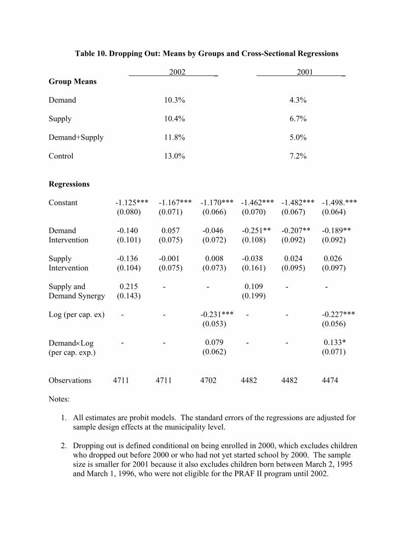
Table 10. Dropping Out: Means by Groups and Cross-Sectional Regressions 2002 _ 2001 _ Group Means Demand 10.3% 4.3% Supply 10.4% 6.7% Demand+Supply 11.8% 5.0% Control 13.0% 7.2% Regressions Constant -1.125***

(0.080) -1.167*** (0.071)

-1.170*** (0.066)

-1.462*** (0.070)

-1.482*** (0.067)

-1.498.*** (0.064)

Demand Intervention

-0.140 (0.101)

0.057 (0.075)

-0.046 (0.072)

-0.251** (0.108)

-0.207** (0.092)

-0.189** (0.092)

Supply Intervention

-0.136 (0.104)

-0.001 (0.075)

0.008 (0.073)

-0.038 (0.161)

0.024 (0.095)

0.026 (0.097)

Supply and Demand Synergy

0.215 (0.143)

- - 0.109 (0.199)

- -

Log (per cap. ex) - - -0.231***

(0.053) - - -0.227***

(0.056) Demand×Log (per cap. exp.)

- - 0.079 (0.062)

- - 0.133* (0.071)

Observations 4711 4711 4702 4482 4482 4474 Notes:

1. All estimates are probit models. The standard errors of the regressions are adjusted for sample design effects at the municipality level.

2. Dropping out is defined conditional on being enrolled in 2000, which excludes children

who dropped out before 2000 or who had not yet started school by 2000. The sample size is smaller for 2001 because it also excludes children born between March 2, 1995 and March 1, 1996, who were not eligible for the PRAF II program until 2002.

Table 11. Days Absent: Means by Groups and Cross-Sectional Regressions 2002 _ Group Means Demand 1.25 Supply 1.52 Demand+Supply 1.15 Control 2.00 Regressions Constant 0.269***

(0.061) 0.303***

(0.056) 0.302*** (0.055)

Demand Intervention -0.274***

(0.085) -0.207*** (0.063)

-0.204*** (0.063)

Supply Intervention -0.213**

(0.093) -0.104* (0.063)

-0.103* (0.060)

Supply and Demand Synergy 0.176

(0.121) - -

Log (per cap. ex) - - -0.067*

(0.040)

Demand×Log (per cap. exp.) - - 0.020

(0.048)

Observations 5454 5454 5443 Notes:

1. All estimates are ordered probit models. The standard errors of the regressions are adjusted for sample design effects at the municipality level.

2. All regressions are for 2002 only and are conditional on current enrollment. The

dependent variable is days absent in the last month. The sample excludes children born between March 2, 1986 and March 1, 1987, who were not eligible for the PRAF II program in 2002 because they were 13 years old on March 1, 2002.

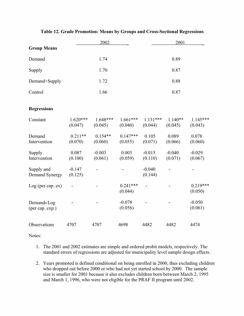
Table 12. Grade Promotion: Means by Groups and Cross-Sectional Regressions 2002 _ 2001 _ Group Means Demand 1.74 0.89 Supply 1.70 0.87 Demand+Supply 1.72 0.88 Control 1.66 0.87 Regressions Constant 1.620***

(0.047) 1.648***

(0.045) 1.661*** (0.040)

1.131*** (0.044)

1.140** (0.045)

1.145*** (0.043)

Demand Intervention

0.211** (0.070)

0.154** (0.060)

0.147*** (0.055)

0.105 (0.071)

0.089 (0.066)

0.078 (0.060)

Supply Intervention

0.087 (0.100)

-0.003 (0.061)

0.003 (0.059)

-0.015 (0.110)

-0.040 (0.071)

-0.029 (0.067)

Supply and Demand Synergy

-0.147 (0.125)

- - -0.040 (0.144)

- -

Log (per cap. ex) - - 0.241***

(0.044) - - 0.219***

(0.050) Demand×Log (per cap. exp.)

- - -0.078 (0.056)

- - -0.050 (0.061)

Observations 4707 4707 4698 4482 4482 4474 Notes:

1. The 2001 and 2002 estimates are simple and ordered probit models, respectively. The standard errors of regressions are adjusted for municipality level sample design effects.

2. Years promoted is defined conditional on being enrolled in 2000, thus excluding children

who dropped out before 2000 or who had not yet started school by 2000. The sample size is smaller for 2001 because it also excludes children born between March 2, 1995 and March 1, 1996, who were not eligible for the PRAF II program until 2002.

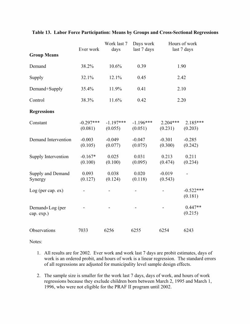
Table 13. Labor Force Participation: Means by Groups and Cross-Sectional Regressions

Ever work

Work last 7

days

Days work last 7 days

Hours of work

last 7 days

Group Means Demand 38.2% 10.6% 0.39 1.90 Supply 32.1% 12.1% 0.45 2.42 Demand+Supply 35.4% 11.9% 0.41 2.10 Control 38.3% 11.6% 0.42 2.20 Regressions Constant -0.297***

(0.081) -1.197*** (0.055)

-1.196*** (0.051)

2.204*** (0.231)

2.185*** (0.203)

Demand Intervention -0.003

(0.105) -0.049 (0.077)

-0.047 (0.075)

-0.301 (0.300)

-0.285 (0.242)

Supply Intervention -0.167*

(0.100) 0.025

(0.100) 0.031

(0.095) 0.213

(0.474) 0.211

(0.234)

Supply and Demand Synergy

0.093 (0.127)

0.038 (0.124)

0.020 (0.118)

-0.019 (0.543)

-

Log (per cap. ex) - - - - -0.522***

(0.181)

Demand×Log (per cap. exp.)

- - - - 0.447** (0.215)

Observations 7033 6256 6255 6254 6243 Notes:

1. All results are for 2002. Ever work and work last 7 days are probit estimates, days of work is an ordered probit, and hours of work is a linear regression. The standard errors of all regressions are adjusted for municipality level sample design effects.

2. The sample size is smaller for the work last 7 days, days of work, and hours of work

regressions because they exclude children born between March 2, 1995 and March 1, 1996, who were not eligible for the PRAF II program until 2002.

Table 14. Enrollment: Means and Regressions over Time

2000 to 2002 _ 2000 to 2001 _ Change in Group Means Demand +17.7% +11.9% Supply +16.9% +9.9% Demand+Supply +15.8% +10.6% Control +15.1% +9.8% Regressions Constant 0.368***

(0.059) 0.389***

(0.057) 0.542***

(0.065) 0.568***

(0.062)

Demand Intervention (βOD) 0.110

(0.080) 0.091

(0.074) 0.162*

(0.087) 0.147*

(0.083)

Supply Intervention (βOS) 0.017

(0.080) 0.022

(0.076) 0.042

(0.089) 0.050

(0.086)

Time Trend (βt) 0.482***

(0.054) 0.489***

(0.054) 0.323***

(0.035) 0.332***

(0.035)

Time×Demand Intervention (βOD, t)

0.093 (0.065)

0.086 (0.066)

0.125*** (0.046)

0.118** (0.047)

Time×Supply Intervention (βOS, t)

-0.012 (0.066)

-0.012 (0.067)

-0.016 (0.047)

-0.020 (0.048)

Log (per cap. exp.) - 0.270***

(0.038) - 0.277***

(0.045)

Time×Log (per cap. exp.)

- -0.032 (0.034)

- -0.015 (0.032)

Demand Int×Log (per cap. exp.)

- -0.076 (0.048)

- -0.050 (0.056)

Time×Log(per cap. exp.) ×Demand Intervention

- -0.029 (0.043)

- -0.042 (0.039)

Sample Size 14,081 14,057 12,081 12,065

See notes to Table 9 for further explanation.

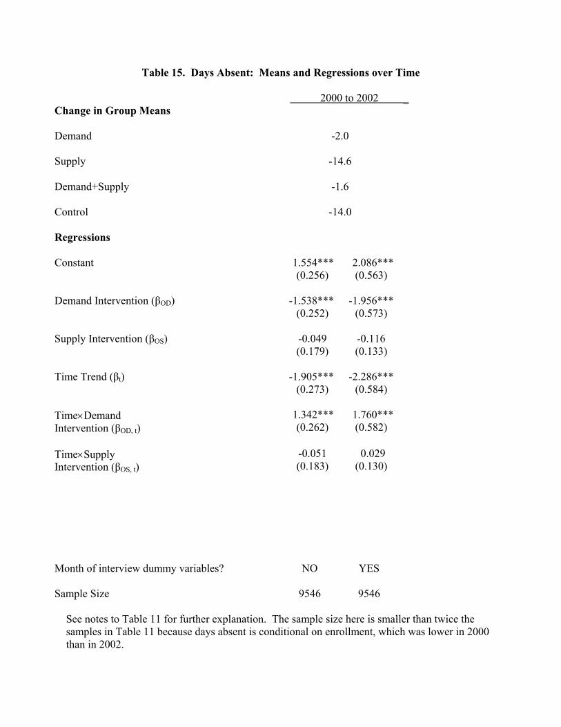
Table 15. Days Absent: Means and Regressions over Time

2000 to 2002 _ Change in Group Means Demand -2.0 Supply -14.6 Demand+Supply -1.6 Control -14.0 Regressions Constant 1.554***

(0.256) 2.086*** (0.563)

Demand Intervention (βOD) -1.538***

(0.252) -1.956***

(0.573)

Supply Intervention (βOS) -0.049

(0.179) -0.116 (0.133)

Time Trend (βt) -1.905***

(0.273) -2.286***

(0.584)

Time×Demand Intervention (βOD, t)

1.342*** (0.262)

1.760*** (0.582)

Time×Supply Intervention (βOS, t)

-0.051 (0.183)

0.029 (0.130)

Month of interview dummy variables? NO YES Sample Size 9546 9546

See notes to Table 11 for further explanation. The sample size here is smaller than twice the samples in Table 11 because days absent is conditional on enrollment, which was lower in 2000 than in 2002.

Table 16. Grade Promotion: Means and Regressions over Time

2000 to 2002 _ 2000 to 2001 _ Change in Group Means Demand +0.083 +0.101 Supply +0.009 +0.031 Demand+Supply +0.051 +0.070 Control +0.020 +0.061 Regressions Constant 0.618***

(0.034) 0.617*** (0.035)

0.885*** (0.052)

0.877*** (0.053)

Demand Intervention (βOD) -0.047

(0.036) -0.050 (0.037)

-0.081 (0.063)

-0.083 (0.064)

Supply Intervention (βOS) 0.048

(0.037) 0.050

(0.037) 0.083

(0.065) 0.087

(0.063)

Time Trend (βt) 1.887***

(0.071) 1.900*** (0.066)

0.254*** (0.058)

0.268*** (0.054)

Time×Demand Intervention (βOD, t)

0.231*** (0.068)

0.229*** (0.065)

0.170** (0.071)

0.161** (0.068)

Time×Supply Intervention (βOS, t)

-0.051 (0.064)

-0.048 (0.062)

-0.122* (0.068)

-0.115* (0.065)

Log (per cap. exp.) - 0.063***

(0.022) - 0.118***

(0.041)

Time×Log (per cap. exp.)

- 0.223*** (0.052)

- 0.100* (0.062)

Demand Int×Log (per cap. exp.)

- 0.013 (0.030)

- 0.016 (0.056)

Time×Log(per cap. exp.) ×Demand Intervention

- -0.108* (0.065)

- -0.066 (0.078)

Sample Size 7699 7685 7475 7462

See notes to Table 12. The sample sizes are less than double those in Table 12 because

enrollment rates in 1999 were lower than in 2000 for the children in the sample.

Table 17. Labor Force Participation: Means and Regressions over Time

Work last 7 days? Hours of work last 7 days Change in Group Means Demand +3.2% +0.03 Supply -8.1% -2.33 Demand+Supply +4.6% +0.16 Control -3.5% -1.80 Regressions Constant -0.997***

(0.076) -1.198** (0.568)

4.137*** (0.553)

2.179 (5.231)

Demand Intervention (βOD) -0.501***

(0.097) -0.196 (0.564)

-2.398*** (0.610)

-0.314 (5.209)

Supply Intervention (βOS) 0.097

(0.100) 0.065

(0.085) 0.333

(0.540) 0.160

(0.465)

Time Trend (βt) -0.207**

(0.092) 0.017

(0.573) -1.929***

(0.573) -0.040 (5.207)

Time×Demand Intervention (βOD, t)

0.468*** (0.121)

0.162 (0.572)

2.090*** (0.658)

0.029 (5.205)

Time×Supply Intervention (βOS, t)

0.049 (0.124)

-0.023 (0.109)

-0.133 (0.591)

0.090 (0.535)

Month of interview dummy variables?

NO YES NO YES

Sample Size 11,302 11,302 11,323 11,323

See notes to Table 13. Note that the sample sizes are less than double those in Table 13 because children in the sample who were four or five years old in 2000 were not asked questions about labor force participation

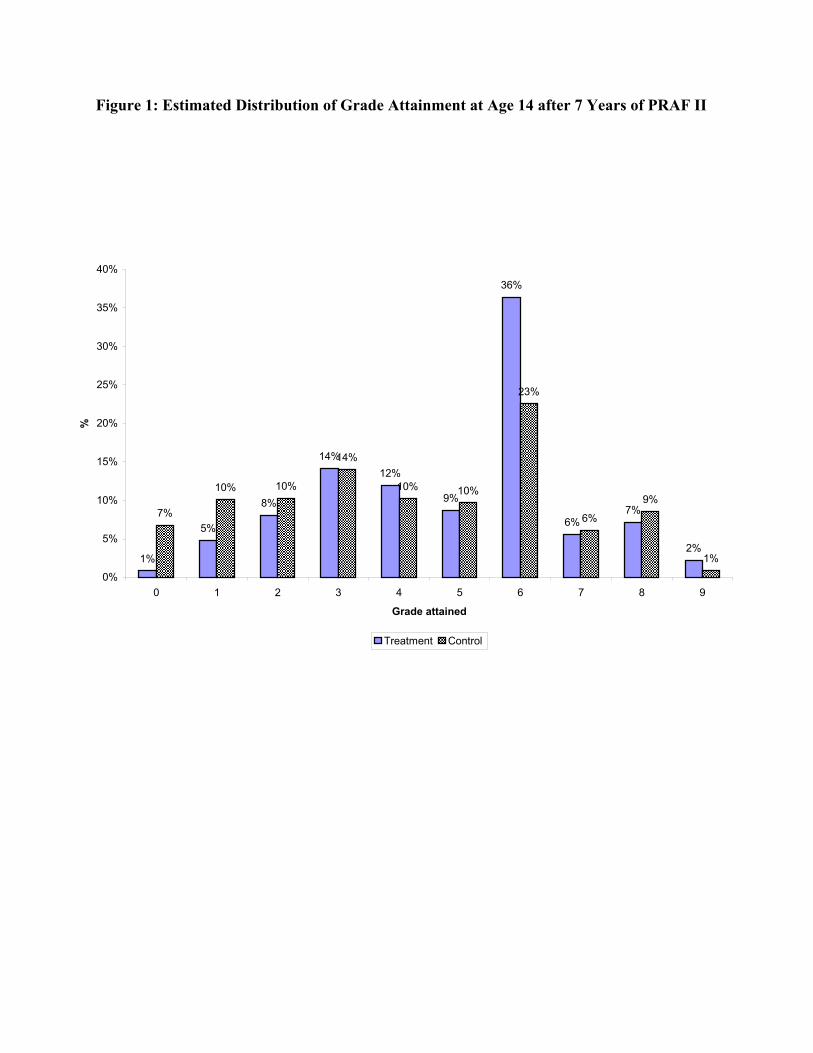
Figure 1: Estimated Distribution of Grade Attainment at Age 14 after 7 Years of PRAF II

����������������������������

������������������������������������������������

������������������������������������������������

����������������������������������������������������������������

������������������������������������������

�����������������������������������

������������������������������������������������������������������������������������������������

��������������������������������

���������������������������������������� �������1%

5%

8%

14%12%

9%

36%

6%7%

2%

7%

10% 10%

14%

10% 10%

23%

6%

9%

1%

0%

5%

10%

15%

20%

25%

30%

35%

40%

0 1 2 3 4 5 6 7 8 9

Grade attained

%

Treatment

��������Control

Figure 2: Estimated Cumulative Distribution of Grade Attainment at Age 14 after 7 years

of Exposure to PRAF II

0.00

0.20

0.40

0.60

0.80

1.00

0 1 2 3 4 5 6 7 8 9

dem dem inf dem sup con con inf con sup