Evaluating Interest Rate Covariance Models within a

Value-at-Risk Framework∗

Miguel A. Ferreira†

ISCTE Business School-Lisbon

Jose A. Lopez‡

Federal Reserve Bank of San Francisco

∗Please note that the views expressed here are those of the authors and not necessarily of the Federal Reserve Bankof San Francisco or of the Federal Reserve System. We thank seminar participants at the 2003 Center for FinancialResearch conference on New Directions in Financial Risk Management as well as the editors and two anonymousreferees for their comments.

†Address: ISCTE Business School - Lisbon, Complexo INDEG/ISCTE, Av. Prof. Anibal Bettencourt, 1600-189Lisboa, Portugal. Phone: 351 21 7958607. Fax: 351 21 7958605. E-mail: miguel.ferreira@iscte.pt.

‡Corresponding author address: Economic Research Department Group Risk Management, Federal Reserve Bankof San Francisco, 101 Market Street, San Francisco, CA 94705. Phone: (415) 977-3894. Fax: (415) 974-2168. E-mail:jose.a.lopez@sf.frb.org.

1

Abstract

A key component of managing international interest rate portfolios is forecasts of the covariances

between national interest rates and accompanying exchange rates. How should portfolio managers

choose among the large number of covariance forecasting models available? We find that covariance

matrix forecasts generated by models incorporating interest-rate level volatility effects perform best

with respect to statistical loss functions. However, within a value-at-risk (VaR) framework, the rel-

ative performance of the covariance matrix forecasts depends greatly on the VaR distributional

assumption, and forecasts based just on weighted averages of past observations perform best. In

addition, portfolio variance forecasts that ignore the covariance matrix generate the lowest regu-

latory capital charge, a key economic decision variable for commercial banks. Our results provide

empirical support for the commonly-used VaR models based on simple covariance matrix forecasts

and distributional assumptions.

JEL classification: C52; C53; G12; E43

Keywords: Interest rates; Covariance models; GARCH; Forecasting; Risk Management; Value-at-

Risk

2

The short-term interest rate is one of the most important and fundamental variables in financial

markets. In particular, interest rate volatility and its forecasts are important to a wide variety of

economic agents. Portfolio managers require such volatility forecasts for asset allocation decisions;

option traders require them to price and hedge interest rate derivatives; and risk managers use

them to compute measures of portfolio market risk, such as value-at-risk (VaR). In fact, since

the late 1990s, financial regulators have been using VaR methods and their underlying volatility

forecasts to monitor specific interest rate exposures of financial institutions.

Forecasts of interest rate volatility are available from two general sources. The market-based

approach uses option market data to infer implied volatility, which is interpreted to be the market’s

best estimate of future volatility conditional on an option pricing model. Since these forecasts

incorporate the expectations of market participants, they are said to be forward-looking measures.

The model-based approach forecasts volatility from time series data, generating what are usually

called historical forecasts. The empirical evidence in Day and Lewis (1992), Amin and Ng (1997),

and others suggests that implied volatility can forecast future volatility. However, there is also

some consensus that implied volatility is an upward biased forecast of future volatility and that

historical volatility forecasts contain additional useful information. Moreover, the scope of available

implied second moments is limited due to options contracts availability, especially with respect to

covariances.1

Much of the work on the model-based approach to forecast second moments has focused on

univariate time-varying variance models; see Bollerslev, Engle, and Nelson (1994). In practice, given

the large number of models available, how should portfolio managers choose among them?2 Most

studies evaluate the performance of such volatility models using in-sample analysis. However, out-

of-sample evaluation of forecasts provides a potentially more useful comparison of the alternative

models, due to the possibility of overfitting. Moreover, the ability to produce useful out-of-sample

forecasts is a clear test of model performance because it only uses the same information set available

to agents at each point in time.3 Previous studies across several financial markets have compared

the out-of-sample forecasting ability of several GARCH type models with that of simple variance

measures and found that there is no clear winner using statistical loss functions; see for example,

West and Cho (1995), and Andersen and Bollerslev (1998). Figlewski (1997) shows that GARCH

models fitted to daily data may be useful in forecasting stock market volatility both for short

3

and long horizons, but they are much less useful in forecasting volatility in other markets beyond

short horizons.4 In particular, using 3-month US Treasury bill yields, sample variances generate

more accurate forecasts than GARCH model. Ederington and Guan (2000) also find that sample

variances dominate GARCH models in the 3-month Eurodollar market.

In contrast, relatively less work has been done on modeling and forecasting second moments

using multivariate time-varying covariance models. For example, Kroner and Ng (1998) propose a

general family of multivariate GARCH models, called General Dynamic Covariance (GDC) model,

and Engle (2002) proposes the dynamic conditional correlation (DCC) model that is a generalization

of the constant conditional correlation model of Bollerslev (1990). Focussing on interest rates,

Ferreira (2001) presents a new multivariate model called the GDC-Levels model that includes both

level effects and conditional heteroskedasticity effects in the volatility dynamics.5 He finds that

the interest rate variance-covariance matrix is best forecasted out-of-sample using the multivariate

VECH model with a level effect, although simple models using either equally or exponentially-

weighted moving averages of past observations appear to perform as well under statistical loss

functions.

Given the mixed out-of-sample performance of these models with respect to statistical loss

functions, some studies have compare their out-of-sample performance in terms of a specific eco-

nomic application. Not surprisingly, these results may vary according to the selected economic loss

function; see Lopez (2001). To date, such economic evaluations of out-of-sample volatility fore-

casts has been in the areas of hedging performance, asset allocation decisions, and options pricing.

Regarding hedging strategies, Cecchetti, Cumby, and Figlewski (1988) find that a time-varying

covariance matrix is necessary to construct an optimal hedge ratio between Treasury bonds and

bond futures, while Kroner and Ng (1998) find that the choice of the multivariate specification

can result in very different estimates of the optimal hedge ratio for stock portfolios. With respect

to asset allocation, volatility model selection is also important as shown by Fleming, Kirby, and

Ostdiek (2001), and Poomimars, Cadle, and Theobald (2002). For options pricing, Engle, Kane,

and Noh (1997), Gibson and Boyer (1998), and Byström (2002) find that standard time-series

models produce better correlation forecasts than simple moving average models for the purpose of

stock-index option pricing and trading. Christoffersen and Jacobs (2004) also evaluate alternative

GARCH covariance forecasts in terms of option pricing and find out-of-sample evidence in favor of

4

relatively parsimonious models.

In this paper, we consider economic loss functions related to financial risk management and

based on value-at-risk (VaR) measures that generally indicate the amount of portfolio value that

could be lost over a given time horizon with a specified probability. Hendricks (1996) provides an

extensive evaluation of alternative VaR models using a portfolio of foreign exchange rates, although

he does not examine covariance matrix forecasts. Other papers - Alexander and Leigh (1997),

Jackson, Maude, and Perraudin (1997), Brooks, Henry, and Persand (2002), Brooks and Persand

(2003), and Wong, Cheng, and Wong (2003) - examine VaR measures for different asset portfolios

using multivariate models. We extend this literature by evaluating the forecast performance of

multivariate volatility models within a VaR framework using interest rate data, as per Lopez and

Walter (2001).6

The performance of VaR for interest rate portfolios, one of the most important financial prices

and of particular relevance in banks’ trading portfolios, is studied using univariate models by Vlaar

(2000), who examines the out-of-sample forecast accuracy of several univariate volatility models for

portfolios of Dutch government bonds with different maturities. In addition, he examines the im-

pact of alternative VaR distributional assumptions. The analysis shows that the percentage of VaR

exceedances for simple models is basically equal to that for GARCH models. The distributional

assumption is also important with the normal performing much better than the t-distribution.

Brooks and Persand (2003) examine FTA British Government Bond Index and find that multivari-

ate GARCH models do not contribute much under standard statistical loss functions and certain

VaR evaluation measures.

Our study considers an equally-weighted portfolio of short-term fixed income positions in the

US dollar, German deutschemark and Japanese yen. The portfolio returns are calculated from the

perspective of a US-based investor using daily interest rate and foreign exchange data from 1979

through 2000. We examine VaR estimates for this portfolio from a wider variety of multivariate

volatility models, ranging from simple sample averages to standard time-series models. We compare

the out-of-sample forecasting performance of these alternative variance-covariance structures and

their economic implications within the VaR framework used by Lopez and Walter (2001). The

question of interest is whether more complex covariance models provide improved out-of-sample

VaR forecasts.

5

The VaR framework consists of three sets of evaluation techniques. The first set focuses on the

statistical properties of VaR estimates derived from alternative covariance matrix forecasts and VaR

distributional assumptions. Specifically, the binomial test of correct unconditional and conditional

coverage, which is implicitly incorporated into the aforementioned bank capital requirements, is

used to examine 1%, 5%, 10%, and 25% VaR estimates. The second set of techniques focus on the

magnitude of the losses experienced when VaR estimates are exceeded. To determine whether the

magnitudes of observed exceptions are in keeping with the model generating the VaR estimates,

we use the hypothesis test based on the truncated normal distribution proposed by Berkowitz

(2001). Finally, to examine the performance of the competing covariance matrix forecasts with

respect to regulatory capital requirements, we use the regulatory loss function implied by the U.S.

implementation of the market risk amendment to the Basel Capital Accord. This loss function

penalizes a VaR model for poor performance by using a capital charge multiplier based on the

number of VaR exceptions; see Lopez (1999a) for further discussion.

Our findings are roughly in line with those of Lopez and Walter (2001), which are based on a

simple portfolio of foreign exchange positions. As per Ferreira (2001), we confirm that covariance

matrix forecasts generated from models that incorporate interest-rate level effects perform best

under statistical loss functions. However, simple specifications, such as weighted averages of past

observations, perform best with regard to the magnitude of VaR exceptions and regulatory capital

requirements.

We also find that the relative performance of covariance matrix forecasts depends greatly on

the VaR models’ distributional assumptions. Our results provide further empirical support for

the commonly-used VaR models based on simple covariance matrix forecasts and distributional

assumptions, such as the normal and nonparametric distributions. Moreover, simple variance fore-

casts based only on the portfolio returns (i.e., ignoring the portfolio’s component assets) perform

as well as the best covariance matrix forecasts and, in fact, generate the minimum capital require-

ments in our exercise. This finding is mainly consistent with the evidence in Berkowitz and O’Brien

(2002), who analyzed the daily trading revenues and VaR estimates of six US commercial banks.

They find that a GARCH model of portfolio returns that ignores the component assets, when

combined with a normal distributional assumption, provides VaR estimates and regulatory capital

requirements that are comparable to other models and does not produce large VaR exceptions.

6

The paper is structured as follows. Section 1 describes the issue of forecasting variances and

covariances and presents the alternative time-varying covariance specifications. We also compare

the models in terms of out-of-sample forecasting power for variances and covariances. Section 2

describes the VaR models analyzed. Section 3 presents the results for the hypothesis tests that

make up the VaR evaluation framework. Section 4 concludes.

1 Time-Varying Covariance Models

In this paper, we study an equally-weighted US dollar-denominated portfolio of US dollar (US$),

Deutschemark (DM), and Japanese yen (JY) short-term interest rates. We take the view of a US-

based investor, who is unhedged with respect to exchange rate risk. Thus, we need to estimate the

(5×5) variance-covariance matrix between the three interest rates as well as DM/US$ and JY/US$exchange rates.

1.1 Forecasting Variances and Covariances

The standard empirical model for the short-term interest rate rit for i =US$,DM,JY is

rit − rit−1 = µi + κirit−1 + εit, (1)

and the standard model for the foreign exchange rate sit for i =DM/US$,JY/US$ is

logµsitsit−1

¶= εit, (2)

where E [εit|Ft−1] = 0 and Ft−1 is the information set up to time t − 1. The conditional meanfunction for the interest rate in (1) is given by a first-order autoregressive process, and we assume

a zero conditional mean for the continuously compounded foreign exchange rate return in (2). The

conditional variance-covariance matrixHt is (5×5) with elements [hijt] . The conditional covariancesare expressed as

hijt = E [εitεjt|Ft−1] , (3)

and the conditional variances are represented when i = j.

7

The first category of second moment forecasts is based on sample averages of past observations.7

The most common estimator is the equally-weighted sample covariance over a period of T obser-

vations; i.e.,

bhijt = 1

T

T−1Xs=0

εit−sεjt−s. (4)

Note that this forecast assumes that all future values of hijt are constant. The sample covariance

estimator weights equally each past observation included in the estimate. The first set of sample

average forecasts we examine set T = 250 and is denoted as E250.8 The second set of such forecasts

uses all past observations as of time t (i.e., the unconditional estimate at time t) and is denoted as

Eall.

A common feature of financial data is that recent observations have a greater impact on second

moments than older ones. A simple way to incorporate this feature is to weight observations in

inverse relation to their age. The exponentially-weighted sample covariance (EWMA) forecast

assigns more weight to recent observations relative to more distant observations using a weighting

parameter. Let w be the weighting factor (or decay rate) with 0 < w ≤ 1. The forecast formulatedat time t weights all available observations up to that time in the following way:

bhijt = Pt−1s=0w

sεit−sεjt−sPt−1s=0w

s. (5)

In the limit, the forecasts generated by equation (5) include an infinite number of past observations,

but their weights become infinitesimally small.9 The weighting parameter determines the degree

to which more recent data is weighted, and in this study, we assume w = 0.94, which is the value

most commonly used in actual risk management applications.10

We also consider second moment forecasts based directly on portfolio returns, hence ignoring

the covariance matrix completely. This approach significantly reduces computational time and

estimation errors and presents comparable performance in terms of VaR estimates as reported

in Lopez and Walter (2001) and Berkowitz and O’Brien (2002). In particular, we examine the

equally-weighted (with 250 and all past observations) and exponentially-weighted (with a decay

factor of 0.94) sample variance of portfolio returns and denote them as E250-Port, Eall-Port, and

EWMA-Port, respectively. We also consider a GARCH(1,1) variance model of portfolio return,

8

denoted GARCH-Port.

The second category of forecasts we examine explicitly is based on multivariate GARCH models.

In the basic multivariate GARCH model, the components of the conditional variance-covariance

matrix Ht vary through time as functions of the lagged values of Ht and of the squared εt inno-

vations. We model the (5 × 5) covariance matrix of the relevant changes in US$, DM and JP

short-term interest rates as well as DM/US$ and JY/US$ foreign exchange rates using several

multivariate GARCH specifications, as described below.

1.1.1 VECH Model

The VECH model of Bollerslev, Engle, and Wooldridge (1988) is a parsimonious version of the

most general multivariate GARCH model given by, for i, j = 1, 2, ..., 5,

hijt = ωij + βijhijt−1 + αijεit−1εjt−1, (6)

where ωij , βij and αij are parameters. In fact, the VECH model is simply an ARMA process for

εitεjt. An important implementation problem is that the model may not yield a positive definite

Ht covariance matrix. Furthermore, the VECH model does not allow for volatility spillover effects,

i.e., the conditional variance of a given variable is not a function of other variables’ past shocks.

1.1.2 Constant Correlation (CCORR) Model

In the CCORR model of Bollerslev (1990), the conditional covariance is proportional to the product

of the conditional standard deviations; i.e., ρijt = ρij . Consequently, the conditional correlation is

constant across time. The model is described by the following equations, for i, j = 1, 2, ..., 5,

hiit = ωii + βiihiit−1 + αiiε2it−1, hijt = ρij

phiit−1

phjjt−1, for all i 6= j. (7)

The conditional covariance matrix of the CCORR model is positive definite if and only if the

correlation matrix is positive definite. Like in the VECH model there is no volatility spillover

effects across series.

9

1.1.3 Dynamic Conditional Correlation (DCC) Model

The DCC model of Engle (2002) preserves the simplicity of estimation of the CCORR model, but

explicitly allows for time-varying correlations. The Ht covariance matrix model is decomposed as

Ht = DtRtDt, (8)

where Dt is a (5 × 5) diagonal matrix of the individual asset variances hiit given by a univariateGARCH(1,1) specification, and Rt is a time-varying correlation matrix expressed as

Rt = (Q∗t )−1Qt(Q∗t )

−1, (9)

Qt = (1− a− b)Q+ aεt−1ε0t−1 + bQt−1,

where Q is the unconditional covariance of the standardized residuals resulting from the individual

Dt estimations, and Q∗t is a diagonal matrix composed of the square root of the diagonal elements of

Qt. This model generates a positive definite covariance matrix, and there are no volatility spillover

effects across series.

1.1.4 BEKK Model

The BEKK model of Engle and Kroner (1995) is given by:

Ht = Ω+B0Ht−1B +A0εt−1ε0t−1A, (10)

where Ω, A, and B are (5 × 5) matrices, with Ω being symmetric. In the BEKK model, the

conditional covariance matrix is determined by the outer product matrices of the vector of past

innovations. As long as Ω is positive definite, the conditional covariance matrix is also positive

definite because the other terms in (10) are expressed in quadratic form.

1.1.5 General Dynamic Covariance (GDC) Model

The GDC model proposed by Kroner and Ng (1998) nests several multivariate GARCH models.

The conditional covariance specification is given by:

10

Ht = DtRDt +Φ Θt, (11)

where is the Hadamard product operator (element-by-element matrix multiplication), Dt is adiagonal matrix with elements

√θiit, R is the correlation matrix with components ρij , Φ is a

matrix of parameters with components φii = 0 for all i, Θt = [θijt],

θijt = ωij + b0iHt−1bj + a

0iεt−1ε

0t−1aj , for all i, j (12)

ai, bi, i = 1, 2, ..., 5 are (5 × 1) vectors of parameters, and ωij are scalars with Ω ≡ [ωij ] being adiagonal positive definite (5× 5) matrix.

This model combines the constant correlation model with the BEKK model. The first term in

(11) is like the constant correlation model but with variance functions given by the BEKK model.

The second term in (11) has zero diagonal elements with the off-diagonal elements given by the

BEKK model covariance functions scaled by the φij parameters. Thus, the GDC model structure

can be written as follows:

hiit = θiit (13)

hijt = ρijpθiitpθjjt + φijθijt for all i 6= j.

The GDC model nests the multivariate GARCH models discussed above.11 The VECH model

assumes that ρij = 0 for all i 6= j.12 The BEKK model has the restrictions ρij = 0 for all i 6= j andφij = 1 for all i 6= j. The CCORR model considers φij = 0 for all i 6= j.

1.1.6 GDC-Levels (GDC-L) Model

One of the most important features of the short-term interest rate volatility is the level effect; i.e.,

volatility is a function of the interest rate level. Chan, Karolyi, Longstaff, and Sanders (1992)

document this effect using a conditional variance specification where only the interest rate level

drives the evolution of the interest rate volatility. They find that the sensitivity of interest rate

variance to the interest rate level is very high and in excess of unity. Subsequent work by Brenner,

11

Harjes, and Kroner (1996) shows that the level effect exists, but it is considerably smaller (i.e.,

consistent with a square root process) by incorporating into the variance function both level and

conditionally heteroskedasticity effects (i.e., news effect) using a GARCH framework. Bali (2003)

also finds that incorporating both GARCH and level effects into the interest rate volatility improves

the pricing performance of the models.

We consider a multivariate version of the Brenner et al. (1996) model by extending the GDC

model to incorporate the level effect in the variance-covariance functions for the interest rates, but

not for the exchange rates. That is, we specify

θijt = ω∗ij + b0iH

∗t−1bj + a

0iε∗t−1ε

∗0t−1aj , for i, j = 1, 2, 3 (14)

where ω∗ii = ωii/r2γiit−1, the diagonal elements of the matrix H

∗t−1 are multiplied by the factor

(rit−1/rit−2)2γi for all i, and the elements of the vector ε∗t−1 are divided by rγiit−1 for all i. The

GDC-Levels model nests the prior multivariate GARCH models and introduces the level effect.

For the sake of completeness, we also introduce the level effect specification into our other

multivariate GARCH models. The exact form of conditional variance in the VECH model with

level effect, denoted the VECH-L model for the interest rate is given by:

hiit =³ωii + βiihiit−1r

−2γiit−2 + αiiε

2it−1

´r2γiit−1. (15)

Similarly, we construct the CCORR-L, DCC-L and BEKK-L models. In summary, a total of

seventeen volatility forecasting models are analyzed below.

1.2 Models Estimation

1.2.1 Data Description

The daily interest rate data examined here are US dollar (US$), Deutschemark (DM) and Japanese

yen (JY) three-month money market interest rates from the London interbank market.13 The

interest rates are given in percentage and in annualized form. These interest rates are taken as

proxies for the instantaneous riskless interest rate (i.e., the short rate) as per Chapman, Long, and

Pearson (1999). We also require foreign exchange rates to compute U.S. dollar investor rates of

12

return, and the JY/US$ and DM/US$ spot exchange rates used here are from the London market.14

As in most of the literature, we focus on nominal interest rates because generating real inter-

est rates at high frequencies is subject to serious measurement errors. The use of daily frequency

minimizes the discretization bias resulting from estimating a continuous-time process using discrete

periods between observations. We use interbank interest rates in our work, instead of government

securities yields, because of the lesser liquidity of these secondary markets in Germany and Japan,

which is in sharp contrast with the high liquidity of the interbank money market. Concerns re-

garding the existence of a default premium in the interbank money market should not be material

since these interest rates result from trades among highly-rated banks that are considered almost

default-free at short maturities.

The period of analysis is from January 12, 1979 to December 29, 2000, providing 5731 daily

observations. Table 1 presents summary statistics for the interest rate first differences and foreign

exchange rate geometric return. The mean interest rate changes are all close to zero, while the

standard deviations differ considerably with the US interest rate changes having an annualized

standard deviation of 2.8% compared with 1.8% and 1.4% for the Japanese and German interest

rate changes, respectively. The daily exchange rate changes are also close to zero, but they present a

much higher degree of variation with an annualized standard deviation of about 11% for both series.

Table 1 also presents summary statistics for an equally-weighted portfolio of the US$, DM and JY

interest rates with returns calculated in US$; see section 2 for a detailed portfolio return definition.

The mean portfolio return is almost zero with an annualized standard deviation of 19.6%. The

portfolio return presents leptokurtosis, though less severe that most individual components series,

with exception of the DM/US$ exchange rate return.

Figure 1 plots the daily time series of US$, DM, and JY three-month interest rates as well

as the DM/US$ and JY/US$ foreign exchange rates. Both daily interest rates (foreign exchange

rates) levels and first differences (geometric returns) are plotted. The daily time series of portfolio

returns is also plotted. All three interest rate series present a downward trend over the sample

period. However, the DM and JY interest rate present a sharp increase in the early 1990s. The

US$ foreign exchange rate presents a steady depreciation after the mid 1980s, when it reached a

peak against both the DM and JY.

13

1.2.2 Forecasting Performance

The multivariate model parameters are estimated using a rolling scheme; i.e., parameters are rees-

timated using a fixed window of 2861 daily observations (or approximately ten years of data) and

updated once every year. For example, the first estimation period is from January 12, 1979 to

December 29, 1989 to calculate the models’ one-step-ahead variance-covariance forecasts over the

out-of-sample period from January 1, 1990 to December 31, 1990. The overall out-of-sample period

is from January 1, 1990 to December 29, 2000. 15

Following standard practice, we estimate the models by maximizing the likelihood function

under the assumption of independent and identically distributed (i.i.d.) innovations. In addition, we

assume that the conditional density function of the innovations is given by the normal distribution.

Conditional normality of the innovations is often difficult to justify in many empirical applications

that use leptokurtic financial data, as shown for our data in Table 1. However, the maximum

likelihood estimator based on the normal density has a valid quasi-maximum likelihood (QML)

interpretation as shown by Bollerslev and Wooldridge (1992).16

Tables 2 and 3 present the various models’ out-of-sample forecast performance in terms of

mean prediction error (MPE) and root mean squared prediction error (RMPSE). Table 2 reports

MPE and RMSPE for the variances of the five component assets and the overall portfolio, and

Table 3 reports MPE and RMSPE for the ten relevant covariances. We also report Diebold and

Mariano (1995) test statistics comparing the models’ forecasting accuracy relative to the one with

the minimum RMSPE.

These results suggest a slight bias, as measured by MPE, toward overestimating both variances

and covariances. Only the JY/US$ exchange rate variance is underestimated by most models.

Accordingly, the portfolio variance is overestimated by most models.

Overall, the results in Tables 2 and 3 clearly indicate that no single model dominates the others

in terms of the RMSPE loss function. Across the 15 forecasted second moments, 10 different

models of the 13 models examined generated the lowest RMSPE values at least once. Based on the

Diebold-Mariano test results, we observe that in many cases we cannot reject the null hypothesis

of equal forecast accuracy for the RMSPE-minimizing forecasts and the alternative forecasts.

Based on these results, the best performing model across the 15 moments is the VECH-L model,

14

which minimizes RMSPE in three cases and is never rejected as less accurate than other models.

Notably, the VECH model performs only slightly worse as it is the RMSPE-minimizing forecast in

two cases and rejected the equal accuracy hypothesis only once. This result, in conjunction with the

comparative performance of the models with and without interest rate level effects, suggests that

the level effect does not contribute to out-of-sample performance here. In addition, the performance

of the simple models is quite reasonable given their lack of explicit time dynamics. The sample

variance of the past 250 day observations (E250 model) performs similarly to the best multivariate

models, especially in terms of covariance. The equal accuracy hypothesis is only rejected at the 5%

level in five cases, and it is the RMSPE minimizing forecast in three cases

Portfolio variance is best forecasted by the VECH and VECH-Levels models, confirming their

performance in forecasting the individual variances and covariances. For the portfolio variance

forecasts based solely on the portfolio returns, the null hypothesis of equal forecasting power relative

to the best model is not rejected at the 5% level for the GARCH-Port and EWMA-Port models.

This result suggests that simple portfolio variance forecasts are useful, even though full covariance

matrix forecasts generally perform as well or better. Surprisingly, the E250 model is rejected in

terms of forecasting portfolio variance, in contrast to its good performance for individual variances

and covariances. This comes as a result of the weak performance of this models in terms of

forecasting foreign exchange rate volatilities - an important component of the portfolio variance.

In summary, statistical loss functions provide a useful, although incomplete, analysis of individ-

ual assets’ variance and covariance as well as portfolio variance forecasts. Our results indicate that

the second moment forecasts from simple models and time-varying covariance models present sim-

ilar out-of-sample forecasting performance. In addition, the most complex time-varying covariance

models tend to overfit the data. Our findings are generally consistent with those of Ferreira (2001)

for interest rates, and West and Cho (1995) and Lopez (2001) for foreign exchange rates. However,

economic loss functions that explicitly incorporate the costs faced by volatility forecast users pro-

vide the most meaningful forecast evaluations. In the next section, we examine the performance of

the covariance matrix forecasts within a value-at-risk framework.

15

2 Value-at-Risk Framework

2.1 Portfolio Definition

Assume that we have a US fixed-income investor managing positions in US$, DM, and JY three-

month zero-coupon bonds in terms of dollar-denominated returns.17 From the perspective of a

US-based investor, define the value of a US$ investment tomorrow to be

YUS$t+1 = YUS$teRUS$t+1 , (16)

where RUS$t+1 = −14 (rUS$t+1 − rUS$t) denotes the day t+ 1 geometric rate of return on the three-month zero-coupon bond investment and rUS$t is the annualized US$ three-month interest rate

(continuously compounded).

The value of the DM zero-coupon bond in US$ tomorrow is given by:

YDMt+1 =¡YDMtsDM/US$t

¢eRDM t+1sUS$/DMt+1, (17)

where sUS$/DMt is the exchange rate between US$ and DM. Thus, the day t+ 1 geometric rate of

return on the DM three-month zero-coupon bond investment given by:

ln (YDMt+1)− ln (YDMt) = RDMt+1 −∆ ln¡sDM/US$t+1

¢, (18)

where RDMt+1 = −14 (rDMt+1 − rDMt) is the local-currency rate of return on the fixed incomeinvestment, rDMt is the annualized DM three-month interest rate (continuously compounded),

and ∆ ln¡sDM/US$t+1

¢=£ln¡sDM/US$t+1

¢− ln ¡sDM/US$t¢¤ is the foreign exchange rate geometricreturn. The analysis for the JY fixed income position is the same as for the DM fixed income.

For simplicity, we will assume that the portfolio at time t is evenly divided between the three

fixed-income positions (equally-weighted portfolio). Thus, the investor’s market risk exposure is

the sum of the three investment returns. That is,

Rpt+1 =

·RUS$t+1 RDMt+1 ∆ ln

¡sDM/US$t+1

¢RJYt+1 ∆ ln

¡sJY/US$t+1

¢ ¸w0, (19)

16

where w =·1 1 −1 1 −1

¸is the portfolio weight vector.

2.2 VaR Models and Exceptions

We examine the accuracy of several VaR models based on different covariance matrix specifications,

as discussed above, and conditional densities. The VaR estimate on day t derived from model m

for a k-day-ahead return, denoted VaRmt(k,α), is the critical value that corresponds to the lower

α percent tail of the forecasted return distribution ft+k; that is,

VaRmt(k,α) = F−1mt+k(α) (20)

where F−1mt+k is the inverse of the cumulative distribution function to fmt+k. In our analysis, a VaR

model m consists of two items: a covariance matrix model and a univariate distributional assump-

tion. Following Lopez and Walter (2001), we separately specify the portfolio variance dynamics

hmpt+1 = w0Hmt+1w, (21)

and the distributional form of fmt+k.18 In terms of portfolio variance dynamics, we consider 10

multivariate covariance model forecasts, three sample variance forecasts and four portfolio variance

forecasts for a total of 17 alternative hmpt+1 specifications. In terms of distributions, we consider

four alternative assumptions: normal, t-student, generalized t-student, and nonparametric distri-

bution. The last distributional form is the unsmoothed distribution of the standardized portfolio

returns residuals, which is the distribution used in the so-called “historical simulation” approach

for generating VaR estimates. This gives a total of 68 VaR models to consider.

The t-distribution assumption requires an estimate of the number of degrees of freedom, which

affects the tail thickness of the distribution. This parameter is estimated using the in-sample stan-

dardized residuals generated by the 17 model specifications. The estimated number of degrees

of freedom ranges from 8 and 11, which correspond to some fat tailedness, and the implied 1%

quantiles range from -2.9 to -2.7 compared with -2.33 for the normal distribution. The generalized

t-distribution assumption requires estimates of two parameters that control the tail thickness and

width of the center of the distribution, named n and q; see Bollerslev et al. (1994). The parameters

17

n and q are also estimated using the in-sample standardized residuals and are found to be in the

ranges of [2.1, 2.5] and [1.0, 1.1], respectively. These estimates imply considerably more fat tailed-

ness than the normal distribution at the 1% quantile, but the opposite is true at higher quantiles.

The nonparametric distribution quantiles are estimated using the unsmoothed distribution of the

standardized portfolio return residuals arising from each of the 17 models. The estimated nonpara-

metric critical values generally present more fat-tailedness at the 1% and 5% quantiles than the

normal distribution, but again the opposite is true at higher quantiles.

The one-day-ahead VaR estimates from model m for the specified fixed-income portfolio at the

α% quantile on day t is

VaRmt (α) =phmpt+1F

−1m (α) , (22)

where we drop the subscript t from the portfolio distribution Fm because we assume that it is

constant over time. We then compare VaRmt (α) to the actual portfolio return on day t + 1,

denoted as Rpt+1. If Rpt+1 <VaRmt (α), then we have an exception. For testing purposes, we

define the exception indicator variable as

Imt+1 =

1 if Rpt+1 < VaRmt (α)

0 if Rpt+1 ≥ VaRmt (α). (23)

2.3 VaR Evaluation Tests

2.3.1 Unconditional and Conditional Coverage Tests

Assuming that a set of VaR estimates and their underlying model are accurate, exceptions can

be modeled as independent draws from a binomial distribution with a probability of occurrence

equal to α percent. Accurate VaR estimates should exhibit the property that their unconditional

coverage bα = x/T equals α percent, where x is the number of exceptions and T the number of

observations. The likelihood ratio statistic for testing whether bα = α is

LRuc = 2hlog³bαx (1− bα)T−x´− log³αx (1− α)T−x

´i, (24)

which has an asymptotic χ2 (1) distribution.19 Note that for this study, finite sample critical values

based on the appropriate parameter values and 100,000 replications are used.

18

The LRuc test is an unconditional test of the coverage of VaR estimates since it simply counts

exceptions over the entire period without reference to the information available at each point in

time. However, if the underlying portfolio returns exhibit time-dependent heteroskedasticity, the

conditional accuracy of VaR estimates is probably a more important issue. In such cases, VaR

models that ignore such variance dynamics will generate VaR estimates that may have correct

unconditional coverage, but at any given time, will have incorrect conditional coverage.

To address this issue, Christoffersen (1998) proposed conditional tests of VaR estimates based

on interval forecasts. VaR estimates are essentially interval forecasts of the lower 1% tail of fmt+1,

the one-step-ahead return distribution. The LRcc test used here is a test of correct conditional

coverage. Since accurate VaR estimates have correct conditional coverage, the Imt+1 variable must

exhibit both correct unconditional coverage and serial independence. The LRcc test is a joint test

of these properties, and the relevant test statistic is LRcc = LRuc+LRind, which is asymptotically

distributed χ2 (2).

The LRind statistic is the likelihood ratio statistic for the null hypothesis of serial independence

against the alternative of first-order Markov dependence.20 The likelihood function under this

alternative hypothesis is

LA = (1− π01)T00 πT0101 (1− π11)

T10 πT1111 , (25)

where the Tij notation denotes the number of observations in state j after having been in state i in

the previous period, π01 = T01/ (T00 + T01) and π11 = T11/ (T10 + T11) . Under the null hypothesis

of independence, π01 = π11 = π, and the likelihood function is

L0 = (1− π)T00+T01 πT01+T11 , (26)

where π = (T01 + T11) /T. The test statistic

LRind = 2 [logLA − logL0] , (27)

has an asymptotic χ2 (1) distribution.

19

2.3.2 Dynamic Quantile Test

We also use the Dynamic Quantile (DQ) test proposed by Engle and Manganelli (2002), which is

a Wald test of the hypothesis that all coefficients as well as the intercept are zero in a regression of

the exception indicator variable on its past values (we use 5 lags) and on current VaR, i.e.,

Imt+1 = δ0 +5Xk=1

δkImt−k+1 + δ6V aRmt + ²t+1. (28)

We estimate the regression model by OLS, and a good model should produce a sequence of unbiased

and uncorrelated Imt+1 variable, so that the explanatory power of this regression should be zero.

Note that here again we use finite sample critical values to test the null hypothesis.

2.3.3 Distribution Forecast Test

Since VaR models are generally characterized by their distribution forecasts of portfolio returns,

several authors have suggested that evaluations should be based directly on these forecasts. Such

an evaluation would use all of the information available in the forecasts. The object of interest in

these evaluation methods is the observed quantile qmt+1, which is the quantile under the distribution

forecast fmt+1 in which the observed portfolio return Rpt+1 actually falls; i.e.,

qmt+1 (Rpt+1) =

Rpt+1Z−∞

fmt+1 (Rp) dRp. (29)

If the underlying VaR model is accurate, then its qmt+1 series should be independent and uniformly

distributed over the unit interval.

Several hypothesis tests have been proposed for testing these two properties, but we use the

likelihood ratio test proposed by Berkowitz (2001).21 For this test, the qmt+1 series is transformed

using the inverse of the standard normal cumulative distribution function; i.e. zmt+1 = Φ−1 (qmt+1) .

If the VaR model is correctly specified, the zmt+1 series should be a series of independent and

identically distributed draws from the standard normal. This hypothesis can be tested against

various alternative specifications, such as

zmt+1 − µm = ρm (zmt − µm) + ηt+1, (30)

20

where the parameters (µm, ρm) are respectively the conditional mean and AR(1) coefficient corre-

sponding to the zmt+1 series, and ηt+1 is a normal random variable with mean zero and variance

σ2m. Under the null hypothesis that both properties are present,¡µm, ρm,σ

2m

¢= (0, 0, 1) . The

appropriate LR statistic is

LRdist = 2£L¡µm, ρm,σ

2m

¢− L (0, 0, 1)¤ , (31)

where L¡µm, ρm,σ

2m

¢is the likelihood function for an AR(1) process with normally distributed

errors including the likelihood for the initial observation. The LRdist statistic is asymptotically

distributed χ2(3), but again finite-sample critical values are used here.

2.3.4 Exception Magnitudes

The evaluation of VaR models, both in practice and in the literature, has generally focused on the

frequency of exceptions and thus has disregarded information on their magnitudes. However, the

magnitudes of exceptions should be of primary interest to the various users of VaR models. To

examine these magnitudes, we use the test of whether the magnitude of observed VaR exceptions

are consistent with the underlying VaR model, as proposed by Berkowitz (2001). The intuition is

that VaR exceptions are treated as continuous random variables, and non-exceptions are treated

as censored random variables. In essence, this test provides a middle ground between the full

distribution approach of the LRdist test and the frequency approach of the LRuc and LRcc tests.

As with the LRdist test, the empirical quantile series is transformed into standard normal zmt+1

series and then treated as censored normal random variables, where the censoring is tied to the

desired coverage level of the VaR estimates. Thus, zmt+1 is transformed into γmt+1 as follows:

γmt+1 =

zmt+1 if zmt+1 < Φ−1 (α)

0 if zmt+1 ≥ Φ−1 (α). (32)

The conditional likelihood function for the right-censored observations of γmt+1 = 0 (i.e., for non-

exceptions) is

f¡γmt+1|zmt+1 ≥ Φ−1 (α)

¢= 1−Φ

µΦ−1 (α)− µm

σm

¶, (33)

21

where µm and σm are respectively the unconditional mean and standard deviation of the zmt+1

series.22 The conditional likelihood function for γmt+1 = zmt+1 is that of a truncated normal

distribution,

f¡γmt+1|zmt+1 < Φ−1 (α)

¢=

φ¡γmt+1

¢Φ³Φ−1(α)−µm

σm

´ . (34)

If the VaR model generating the empirical quantiles is correct, the γmt+1 series should be identically

distributed, and (µm,σm) should equal (0, 1). Thus, the relevant test statistic is

LRmag = 2 [Lmag (µm,σm)− Lmag (0, 1)] , (35)

which is asymptotically distributed χ2(2), although we use finite-sample critical values in our analy-

sis.

2.3.5 Regulatory Loss Function

Under the 1996 Market Risk Amendment (MRA) to the Basel Capital Accord, regulatory capital

for the trading positions of commercial banks is set according to the banks’ own internal VaR

estimates. Given its actual use by market participants, the regulatory loss function implied in the

MRA is a natural way to evaluate the relative performance of VaR estimates within an economic

framework; see Lopez (1999b) for further discussion.

As discussed earlier, our fixed-income portfolio return in US dollars is

Rpt+1 = [ln(YUS$t+1)− ln(YUS$t)] + [ln(YDMt+1)− ln(YDMt)] + [ln(YJYt+1)− ln(YJYt)] (36)

= ln(YUS$t+1YDMt+1YJYt+1)− ln(YUS$tYDMtYJYt),

and the portfolio value in US dollar terms is,

Ypt+1 = YpteRpt+1 (37)

= YUS$t+1YDMt+1YJYt+1.

Replacing Rpt+1 with the one-day-ahead VaR estimate, VaRmt (α), we generate what the portfolio

value is expected to be at the lower α tail of the portfolio return distribution. Hence, the VaR

22

estimate expressed in US dollar terms at time t for period t+ 1 is

VaR$mt (α) = Ypth1− eV aRmt(α)

i. (38)

Note that the path dependence of the portfolio value and of the VaR$mt estimates cannot be

removed and must be accounted for in the calculations. In basic operational terms, we choose a

starting portfolio value and simply track its value over the sample period to carry out the analysis.

The market-risk capital loss function expressed in the MRA is specified as

MRCmt = max·VaR$mt (10, 1) ,

Smt60

59Pk=0

VaR$mt−k (10, 1)¸+ SRmt, (39)

where VaR$mt (10, 1) is the 1% VaR estimate generated on day t for a ten-day holding period and

expressed in dollar ters, Smt is the MRA’s multiplication factor (i.e., from 3 to 4 depending on

the number of exceptions over the past 250 days) and SRmt is a specific risk charge that is not

associated with the VaR modeling (and not examined here). That is, MRCmt is the amount of

regulatory capital a bank must hold with respect to its market risk exposure. The MRA capital

loss function has several elements that reflect the bank regulators’ concerns. First, their focus on

the lower 1% quantile of the banks’ market risk returns suggests a high degree of concern with

extreme portfolio losses.

Second, the use of ten-day VaR estimates reflects the desire of the regulators to impose a ten-day

(or two-week) period during which a bank’s market exposure can be diminished. Instead of using

actual ten-day VaR estimates, it is common for banks and regulators to rely on the simplifying

assumption that one-day VaR estimates can adequately be scaled up using the square root of the

time horizon or, in this case,√10; see Christoffersen, Diebold, and Shuermann (1998) for further

discussion. Hence, the loss function used in our analysis is

MRCmt =√10max

·VaR$mt (1) ,

Smt60

59Pk=0

VaR$mt−k (1)¸. (40)

Third, the max function is used to capture instances when the most recent VaR estimate (in

dollar terms) exceeds its trailing sixty-day average. The objective here is to make sure that the

regulatory capital requirement adjusts quickly to large changes in a bank’s market risk exposure.

23

Finally, the number of exceptions is explicitly included in the capital requirement via the Smt

multiplier in order to assure that banks do not generate inappropriately low VaR estimates.

Under the current framework, Smt ≥ 3, and it is a step function that depends on the numberof exceptions observed over the previous 250 trading days.23 This initial value can be viewed as

a regulatory preference parameter with respect to the degree of market risk exposure within the

banking system. The possible number of exceptions is divided into three zones. Within the green

zone of four or fewer exceptions, a VaR model is deemed “acceptably accurate” to the regulators,

and Smt remains at its minimum value of three. Within the yellow zone of five to nine exceptions,

Smt increases incrementally with the number of exceptions.24 Within the red zone of ten or more

exceptions, the VaR model is deemed to be “inaccurate” for regulatory purposes, and Smt increases

to its maximum value of four. The institution must also explicitly take steps to improve its risk

management system. Thus, banks look to minimize exceptions (in order to minimize the multiplier)

without reporting VaR estimates that are too large and raise the average term in the loss function.

3 VaR Evaluation Results

This section presents the forecast evaluation results of our 68 VaR models. Tables 4 and 5 report,

respectively, mean VaR estimates and the percentage of exceptions observed for each of the models

for the 1%, 5%, 10% and 25% quantiles over the entire out-of-sample period from January 1, 1990

to December 29, 2000. These summary statistics are key components of the VaR evaluation results

reported in Tables 6-13. Both the tables and the discussion below are framed with respect to the

distributional assumption first and then with respect to the relative performance of the 17 models’

second-moment specifications. Note that 13 of the models specify the multivariate dynamics of

the conditional variance-covariance matrix and that four models only specify the dynamics of the

portfolio’s conditional variance.

Table 4 show the mean VaR estimates for our alternative models. The most striking feature

is that the mean VaR estimates depends mainly on the VaR distributional assumption, rather

than on the covariance matrix forecast. The average 1% VaR estimates for the t- and generalized

t-distributions lies outside the first percentile of the portfolio return distribution; see Table 1. In

contrast, the average 1% VaR estimates under the normal distribution is greater than the first

24

percentile of the portfolio return. The nonparametric mean VaR estimate at the 1% quantile is

quite close to the first percentile of the portfolio return for most covariance forecasts.

The observed frequency of exceptions reported in Table 5 confirms that the VaR normal esti-

mates at the 1% quantile are too low, with the observed frequency of exceptions above 1% for all

covariance matrix forecasts. However, at higher quantiles, the normal distribution tend to over-

estimate the VaR estimates. While the t-distribution VaR estimates are too conservative at all

quantiles, the generalized t-distribution VaR estimates do not provide a clear pattern. The non-

parametric distribution assumption VaR estimates perform reasonable well at all quantiles, but

they show a tendency to generate VaR estimates that are too conservative.

3.1 Unconditional and Conditional Coverage Tests

Tables 6 and 7 report results for the unconditional (LRuc) and conditional coverage (LRcc) tests,

respectively. Note that the LRuc and LRcc test results are qualitatively similar. VaR models based

on the standard normal distributional assumption perform relatively well at the 1% quantile, in

that only a few sets of VaR estimates fail the LRuc and LRcc tests at the 5% significance level.

However, almost all fail at the higher quantiles (5%, 10%, and 25%). It is interesting to find that

the standard normal distribution generates VaR estimates that perform well at such a low quantile,

especially since portfolio returns are commonly found to be distributed non-normally, in particular

with fatter tails. This result appears to be in line with those of Lucas (2000), who find that the

upward bias in the estimated dispersion measure under such models (see MPE in Panel A of Tables

2 and 3) appears to partially offset the neglected leptokurtosis.

VaR models based on the t-distribution assumption perform only modestly well for the 1%

quantile, i.e., only about a third of the covariance matrix specifications do not reject the null

hypotheses of the LRuc and LRcc tests. All specifications reject the null hypotheses at the higher

quantiles. Similarly, the results for the VaR models based on the generalized t-distribution, indicate

that most of the covariance matrix specifications fail at the lowest quantile, although they have

some very limited success at the higher quantiles. This result suggests that the tail thickness of

these distributional assumptions probably limits their use to the lowest VaR coverage levels.

The nonparametric distributional results coverage test results provide evidence that these VaR

estimates do relatively well across all four quantiles. For the 1% quantile, all the specifications

25

(except DCC models) do not reject the null hypotheses of correct unconditional and conditional

coverage. While the performance for the 5% quantiles is relatively poor and similar to alternative

distributional assumptions, the performance for the 10% and 25% quantiles is quite reasonable with

non-rejections of the null hypotheses in about 50% and 60% of the cases, respectively.

Although we can conclude that the standard normal and the nonparametric distributional as-

sumptions produce better VaR estimates, inference regarding the relative forecast accuracy of the

13 covariance matrix specifications and four portfolio variance specifications is limited. As shown

in Tables 6 and 7, no strong conclusions can be drawn across the forecasts using these two distri-

butional assumptions, especially at the 1% quantile. Among the multivariate models, the BEKK,

GDC and VECH specifications perform better than the CCORR and DCC specifications. In addi-

tion, there is some evidence that the level effect is important for VaR model performance, especially

for the BEKK and GDC specifications. However, the simple covariance forecasts seem to present

similar performance to the best multivariate models, in particular the EWMA and E250 specifi-

cations. Furthermore, the performance of the univariate portfolio variance specifications suggests

that one could reasonably simplify the generation of VaR estimates by ignoring the underlying

covariance matrix without sacrificing the accuracy of the estimates’ unconditional and conditional

coverage.

In summary, these results indicate that the dominant factor in determining the relative accu-

racy of VaR estimates with respect to coverage is the distributional assumption, which is consistent

with the Lopez and Walter (2001) findings. The specification of the portfolio variance, whether

based on covariance matrix forecasts or univariate forecasts, appears to be of second-order impor-

tance. These results provide support for the common industry practice of using the simple portfolio

variance specifications in generating VaR estimates. However, it does not completely explain why

practitioners have generally settled on the standard normal distributional assumption. Although

it did perform well for the lower coverage levels that are usually of interest, the nonparametric

distribution did relatively better across the four quantiles examined.

3.2 Dynamic Quantile Test

Table 8 presents the results of the VaR estimates evaluation using the Dynamic Quantile test

proposed by Engle and Manganelli (2002). The results are mainly consistent with the ones using

26

the unconditional and conditional coverage tests. In fact, VaR models based on the standard

normal and nonparametric distributional assumption perform relatively well at the 1% quantile.

Under the normal distributional assumption, all but one of the specifications do not reject the null

hypotheses of correct 1% VaR estimates, and the number of rejections under the nonparametric

assumption is just two. Furthermore, the nonparametric distribution presents the best performance

at higher quantiles. The VaR models based on the t-distribution and generalized t-distribution

perform slightly better for the 1% VaR estimates than in the unconditional and conditional coverage

tests, even though the performance is still clearly worse than for the alternative distributional

assumptions. Once again, inference across model specifications is limited due to similar performance

over the various quantiles and distributional assumptions.

3.3 Distribution Forecast Test

Table 9 contains the LRdist test results for the 68 VaR models. These results again show that

the standard normal and the nonparametric distributional assumptions generate VaR estimates

that perform relatively well. The null hypothesis of correct conditional distributional form is not

rejected in about half of these cases. For the entire distribution, the generalized-t distributional

assumption performs equally well, suggesting that these models’ forecasted quantiles closer to the

median perform better than their tail quantiles. The t-distributional assumption again performs

poorly.

These results provide further evidence that the distributional assumption appears to drive

the VaR forecast evaluation results and that the portfolio variance specification is of secondary

importance. Once again, inference on the relative performance of the model specifications is limited.

The clearest result is that the CCORR and DCC specifications reject the null hypothesis in all

cases, while the BEKK and VECH specifications perform best among the multivariate models.

The roughly equivalent performance of the multivariate covariance matrix specifications and the

simple univariate specifications confirms the prior result that one may simplify the VaR calculations

without being penalized in terms of performance.

27

3.4 Exception Magnitudes

The previous tests do not take into account the magnitude of the exceptions, but only their fre-

quency. Analysis of this forecast property should be of clear interest to users of VaR estimates

that must determine actual capital requirements, whether economic or regulatory. In this section,

we analyze model performance by considering the size of the loss when an exception occurs. Table

10 reports the mean exception; i.e., the average loss in excess of the VaR estimate conditional

on the portfolio return being less than the VaR estimate. The mean exception beyond the VaR

estimates is approximately one-half of the portfolio returns’ standard deviation. As expected, the

models based on the t-student distribution generate the lowest mean exceptions, but only at the 1%

quantile. The models based on the normal distribution seem to have the largest mean exceptions

at the 1% quantile, but at the 5% and higher quantiles, they have similar mean exceptions to the

other distributional assumptions. The distributional assumption does not play as large a role with

respect to exception magnitudes as it did for exception frequencies.

The results of the LRmag tests for the four sets of VaR estimates using alternative distributional

assumptions are reported in Table 11. Since this is a joint null hypothesis regarding the exception

frequencies and magnitudes, we should expect it to be rejected for the 191 cases in which the VaR

estimates rejected the binomial null hypothesis alone. This result occurs in 72% (138 of 191) of the

cases with the bulk of the unexpected non-rejections of the joint null hypothesis (33 of 53) occurring

for VaR estimates based on the generalized t-distribution. Overall, the two sets of test results are

in agreement for 66% of the cases (180 of 272), and the joint null hypothesis is rejected after the

binomial null hypothesis is not rejected in another 8% of cases (39 of 272). Thus, the LRmag results

are consistent with the LRuc results in 74% of the cases, which seems to be a reasonable rate of

cross-test correspondence.

The majority of the VaR estimates examined here reject the null hypothesis that the magnitude

of their VaR exceptions are consistent with the model, suggesting that the models are misspecified.

In 65% of the cases (177 of 272), the null hypothesis is rejected. The 95 cases in which the null

hypothesis is not rejected are roughly uniformly distributed across the standard normal, generalized-

t and nonparametic distributional assumptions. As before, the t-distributional assumption performs

poorly, with the null hypothesis rejected in all of its cases. If we only consider the 45 (of 95) cases

28

that pass both the LRuc and the LRmag tests, the nonparametric distribution is represented 62%

(28 of 45) of the time.

Focusing on the different specifications of the portfolio variance forecasts, slightly more inference

across specifications using the LRmag test is possible than under prior tests. Across the three

aforementioned distributional assumptions, four multivariate specification (BEKK-Levels, GDC-

Levels, E250 and EWMA) and two univariate specifications (E250-Port and EWMA-Port) perform

well across all four quantiles. Again, focusing on the 45 specifications that do not reject the null

hypothesis of the LRuc and the LRmag tests, the EWMA-Port specification performs best under

the normal and nonparametric distributional assumptions. However, the multivariate BEKK-Levels

and GDC-Levels specifications as well as the univariate E250-Port specification also perform well,

particularly under the nonparametric assumption.

In summary, distributional assumptions also play an important role in the results of the LRmag

test, as in the other hypothesis tests. However, these results in combination with the the LRuc tests

allow more inference across the portfolio variance specifications, and the results indicate that simple

VaR estimates perform well. Specifically, the VaR estimates based on the EWMA-Port specification,

which ignores the portfolio’s components, performs well across the distributional assumptions and

especially for the nonparametric distribution. This outcome presents further support and validation

for the current use of these simple VaR estimates by financial institutions, if only because of the

lower cost of generating these simple VaR estimates.

3.5 Regulatory Loss Function

As currently specified, the regulatory loss function is based on ten-day VaR estimates at the 1%

quantile. However, since we are examining one-step-ahead portfolio variance forecasts, we evaluate

one-day VaR estimates using this loss function as it is common practice in backtesting procedures.

As this loss function does not correspond to a well-defined statistical test, the EWMA-Normal model

is selected as the benchmark model against which we compare the others. Given the common use

of this model in practice, we choose its capital charges to be the benchmark against which the other

models’ capital charges are compared.

Table 12 presents the percentage of the 2870 out-of-sample trading days for which the MRCmt+1

capital charges for the EWMA-Normal model are less than those of the other 67 VaR models. This

29

model clearly has lower capital requirements than all of the portfolio variance specifications under

the t-distribution and generalized-t distribution with the EWMA-Normal performing better than

these alternatives more than 70% of the time. The only VaR estimates that generates smaller

capital charges than those of the EWMA-Normal model for more than 40% of the trading days are

those of the EWMA-Port model under the normal distribution (EWMA-Port-Normal). Recall that

the EWMA-Port specification completely ignores the covariance matrix dynamics of the portfolios’

component securities.

To more carefully examine these regulatory loss function results, we examine the differences

between the capital charges for the EWMA-Normal model and the other models using the Diebold-

Mariano test statistic. The null hypothesis that we investigate is whether the mean difference

between the two sets of capital charges is equal to zero. If we do not reject the null hypothesis,

then the alternative model performs equally well as the benchmark EWMA-Normal model. If we

reject the null hypothesis and the mean difference is negative, then the EWMA-Normal model and

its VaR estimates perform better because they generate lower capital charges on average. If we

reject the null hypothesis and the mean difference is positive, then the alternative model and its

VaR estimates perform better on average.

Table 12 presents the asymptotic p-values for the Diebold-Mariano statistics. In about 75%

of the cases (50 of 67), we reject the null hypothesis. We reject all the alternative VaR models

based on the t-distribution and generalized-t distributional assumption. For the nonparametric

distribution, we do not reject the null hypothesis for only the BEKK-Levels specification. Under

the normal distribution, for all but one portfolio variance specifications, we do not reject the null

hypothesis, indicating that they perform as well as the EWMA-Normal model under this regulatory

loss function.

The most noteworthy case rejecting the null hypothesis of equal performance is the EWMA-

Port-Normal distribution with lower capital charges than the benchmark model for about 64% of

the trading days. In fact, when the EWMA-Port-Normal model is treated as the benchmark as

shown in Table 13, we reject the null hypothesis in all but 9 cases; all but one case under the normal

distribution. This result implies that these VaR models perform as well as the EWMA-Port-Normal

model under the regulatory loss function, but they generate higher capital charges in more than

50% of the trading days. However, the EWMA-Port-Normal model is much easier to estimate than

30

these other models. Hence, we can clearly state that this simple practitioner model that ignores

the covariance matrix dynamics of the portfolio’s component securities and the fat-tailed nature

of the portfolio returns is the best performing model to use when the objective is to minimize the

MRA regulatory capital requirements.

4 Conclusion

We examine VaR estimates for an international interest rate portfolio using a variety of multivariate

volatility models, ranging from naive averages to standard time-series models. The question of

interest is whether the most complex covariance models provide improved out-of-sample forecasts

for use in VaR analysis.

We find that covariance matrix forecasts generated from models that incorporate interest-rate

level effects perform best under statistical loss functions, such as mean-squared error. Within

a VaR framework, the relative performance of covariance matrix forecasts depends greatly on

the VaR models’ distributional assumptions. Of the forecasts examined, simple specifications,

such as weighted averages of past observations, perform best with regard to the magnitude of

VaR exceptions and regulatory capital requirements. Our results provide empirical support for

the commonly-used VaR models based on simple covariance matrix forecasts and distributional

assumptions, such as the standard normal. Moreover, we find that VaR estimates based on portfolio

variance forecasts that ignore the covariance matrix dynamics of the portfolio’s component securities

and on distributional assumptions that ignore the fat-tailed nature of the portfolio returns perform

best when the objective is to minimize certain regulatory capital requirements.

Overall, our results are consistent with several studies, such as Lopez and Walter (2001),

Berkowitz and O’Brien (2002) and Brooks and Persand (2003), for foreign-exchange rate portfolios,

US commercial bank trading portfolios, and a variety of financial market indexes, respectively. Also,

note that our results closely parallel those of Beltratti and Morana (1999) and Lehar, Scheicher,

and Schittenkopf (2002), who find that volatility forecasts from more complex models perform as

well as those from computationally simpler GARCH models. Similarly, Christoffersen and Jacobs

(2004) find that an objective function based on pricing stock options favors relatively parsimonious

models. Hence, our results are in line with recent other findings that for economic purposes, as ex-

31

pressed via economic loss functions associated with option pricing and risk management, volatility

forecasts from simpler models are found to outperform the forecasts from more complex models.

The reasons for these findings range from the issue of parameter uncertainty, as per Skintzi,

Skiadopoulos, and Refenes (2004), to overfitting the data in-sample. Another potential reason for

our findings is the sensitivity of the relevant economic loss functions (i.e., their first derivatives)

with respect to the volatility forecast inputs. As suggested by Fleming et al. (2001), volatility

forecasts that are smoother than optimal under standard statistical goodness-of-fit criteria are too

variable to perform well under investment loss functions. Similarly, the greater smoothness of the

VaR estimates generated by our EWMA-normal and EWMA-Port-normal models is of value within

our VaR framework.

An interesting paper that addresses this question more directly with respect to VaR estimates

is Lucas (2000), who finds that VaR models based on simple measures of portfolio variance and the

normal distribution generate smaller discrepancies between actual and postulated VaR estimates

than more sophisticated VaR models. He argues that this outcome is based on offsetting biases in

the variance and VaR estimates of simple models that cannot be captured by more sophisticated

models that attempt to capture the actual (but unknown) degree of leptokurtosis in the portfolio

returns. The reasons for our parallel results are worth further study.

32

Figure 1. Time Series of Interest and Foreign Exchange Rates.

The figure plots the daily time series of interest rate and foreign exchange rate levels (black line)

and interest rate first differences, foreign exchange rate geometric returns, and portfolio returns

(grey line) for the sample period between January 12, 1979 and December 29, 2000.

33

References

Alexander, C. O., and C. T. Leigh. (1997). ”On the covariance matrices used in value at risk

models.” Journal of Derivatives 4, 50-62.

Amin, K., and V. Ng. (1997). ”Inferring future volatility from the information in implied volatility

in eurodollar options: A new approach.” Review of Financial Studies 10, 333-367.

Andersen, T., and T. Bollerslev. (1998). ”Answering the skeptics: Yes, standard volatility models

do provide accurate forecasts.” International Economic Review 39, 885-905.

Bali, T. (2003). ”Modeling the stochastic behavior of short-term interest rates: Pricing implications

for discount bonds.” Journal of Banking and Finance 27, 201-228.

Beltratti, A., and C. Morana. (1999). ”Computing value-at-risk with high frequency data.” Journal

of Empirical Finance 6, 431-455.

Berkowitz, J. (2001). ”Testing density forecasts with applications to risk management.” Journal

of Business and Economic Statistics 19, 465-474.

Berkowitz, J., and J. O’Brien. (2002). ”How accurate are value-at-risk models at commercial

banks?.” Journal of Finance 57, 1093-1111.

Bollerslev, T. (1990). ”Modelling the coherence in short-run nominal exchange rates: A multivariate

generalized ARCH model.” Review of Economics and Statistics 72, 498-505.

Bollerslev, T., R. Engle, and D. Nelson. (1994). ”ARCH models.”, In R. Engle and D. McFadden

(eds.), Handbook of Econometrics. Amsterdam, Holland: North-Holland.

Bollerslev, T., R. Engle, and J. Wooldridge. (1988). ”A capital asset pricing model with time-

varying covariances.” Journal of Political Economy 96, 116-131.

Bollerslev, T., and J. M. Wooldridge. (1992). ”Quasi-maximum likelihood estimation and inference

in dynamic models in time-vaying covariances.” Econometric Reviews 11, 143-172.

34

Brenner, R. J., R. Harjes, and K. Kroner. (1996). ”Another look at models of the short-term

interest rate.” Journal of Financial and Quantitative Analysis 31, 85-107.

Brooks, C., O. Henry, and G. Persand. (2002). ”The effect of asymmetries on optimal hedge

ratios.” Journal of Business 75, 333-353.

Brooks, C., and G. Persand. (2003). ”Volatility forecasting for risk management.” Journal of

Forecasting 22, 1-22.

Byström, H. (2002). ”Using simulated currency rainbow options to evaluate covariance matrix

forecasts.” Journal of International Financial Markets, Institutions and Money 12, 216-230.

Campa, J., and K. Chang. (1998). ”The forecasting ability of correlations implied in foreign

exhange options.” Journal of International Money and Finance 17, 855-880.

Cecchetti, S., R. Cumby, and S. Figlewski. (1988). ”Estimation of the optimal futures hedge.”

Review of Economics and Statistics 70, 623-630.

Chan, K., A. Karolyi, F. Longstaff, and A. Sanders. (1992). ”An empirical comparison of alterna-

tive models of short term interest rates.” Journal of Finance 47, 1209-1227.

Chapman, D., J. Long, and N. Pearson. (1999). ”Using proxies for the short rate: When are three

months like an instant?.” Review of Financial Studies 12, 763-806.

Christoffersen, P. (1998). ”Evaluating interval forecasts.” International Economic Review 39, 841-

862.

Christoffersen, P., F. Diebold, and T. Shuermann. (1998). ”Horizon problems and extreme events

in financial risk management.” Economic Policy Review 4, 109-118.

Christoffersen, P., and K. Jacobs. (2004). ”Which GARCH model for option valuation?.” Working

Paper, McGill University; forthcoming in Management Science.

Christoffersen, P., and D. Pelletier. (2004). ”Backtesting value at risk: A duration-based ap-

proach.” Journal of Empirical Finance 9, 343-360.

35

Crnkovic, C., and J. Drachman. (1996). ”Quality control.” Risk 9, 139-143.

Day, T., and C. Lewis. (1992). ”Stock market volatility and the information content of stock index

options.” Journal of Econometrics 52, 267-287.

Diebold, F., T. Gunther, and A. Tay. (1998). ”Evaluating density forecasts with applications to

financial risk management.” International Economic Review 39, 863-883.

Diebold, F., and R. Mariano. (1995). ”Comparing predictice accuracy.” Journal of Business and

Economic Statistics 13, 253-263.

Duffie, D., and K. Singleton. (1997). ”An econometric model of the term structure of interest-rate

swap yields.” Journal of Finance 52, 1287-1321.

Ederington, L., and W. Guan. (2000). ”Forecasting volatility.” Working Paper, Michael F. Price

College of Business, University of Oklahoma.

Engle, R. (2002). ”Dynamic conditional correlation - a simple class of multivariate GARCH mod-

els.” Journal of Business and Economic Statistics 20, 339-350.

Engle, R. (2004). ”Risk and volatility: Econometric models and financial practice.” American

Economic Review 94, 405-420.

Engle, R., and G. Gonzalez-Rivera. (1991). ”Semiparametric ARCH models.” Journal of Business

and Economic Statistics 9, 345-359.

Engle, R., A. Kane, and J. Noh. (1997). ”Index-options pricing with stochastic volatility and the

value of accurate variance forecasts.” Review of Derivatives Research 1, 139-157.

Engle, R., and K. Kroner. (1995). ”Multivariate simultaneous generalized ARCH.” Econometric

Theory 11, 122-150.

Engle, R., and S. Manganelli. (2002). ”CAViaR: Conditional autoregressive value at risk by

regression quantiles.” Working Paper, University of California, San Diego.

36

Ferreira, M. A. (2001). ”Forecasting the comovements of spot interest rates.” Working Paper,

ISCTE Business School, Lisbon; forthcoming in Journal of International Money and Finance.

Figlewski, S. (1997). ”Forecasting volatility.” Financial Markets, Institutions and Instruments 6.

Fleming, J., C. Kirby, and B. Ostdiek. (2001). ”The economic value of volatility timing.” Journal

of Finance 56, 329-352.

Foster, D.P., and D.B. Nelson. (1996). ”Continuous record asymptotics for rolling sample variance

estimators.” Econometrica 64, 139-174.

Gibson, M., and B. Boyer. (1998). ”Evaluating forecasts of correlation using option pricing.”

Journal of Derivatives, Winter, 18-38.

Hendricks, D. (1996). ”Evaluation of value-at-risk models using historical data.” Federal Reserve

Bank of New York Economic Policy Review 2, 39-69.

Jackson, P., D. Maude, and W. Perraudin. (1997). ”Bank capital and value at risk.” Journal of

Derivatives 4, 73-90.

Kroner, K., and V. Ng. (1998). ”Modeling asymmetric comovements of asset returns.” Review of

Financial Studies 11, 817-844.

Kupiec, P. (1995). ”Techniques for verifying the accuracy of risk measurement models.” Journal

of Derivatives 3, 73-84.

Lehar, A., M. Scheicher, and C. Schittenkopf. (2002). ”GARCH vs. stochastic volatility: Option

pricing and risk management.” Journal of Banking and Finance 26, 323-345.

Lopez, J. (1999a). ”Methods for evaluating value-at-risk estimates.” Federal Reserve Bank of San

Francisco Economic Review 2, 3-15.

Lopez, J. (1999b). Regulatory evaluation of value-at-risk models.” Journal of Risk 1, 37-64.

Lopez, J. (2001). ”Evaluating the predictive accuracy of volatility models.” Journal of Forecasting

20, 87-109.

37

Lopez, J., and C.Walter. (2001). ”Evaluating covariance matrix forecasts in a value-at-risk frame-

work.” Journal of Risk 3, 69-98.

Lucas, A. (2000). ”A note on optimal estimation from a risk-management perspective under pos-

sibly misspecified tail behavior.” Journal of Business and Economic Statistics 18, 31-39.

Poomimars, P., J. Cadle, and M. Theobald. (2002). ”Dynamic asset allocation with time-varying

variance-covariance structures.” International Quarterly Journal of Finance 2, 49-68.

Skintzi, V.D., G. Skiadopoulos, and A. P. N. Refenes. (2004). ”The effect of mis-estimating correla-

tion on value-at-risk.” Working Paper, Athens University of Economics and Business; forthcoming

in Journal of Risk.

Vlaar, P. (2000). ”Value at risk models for dutch bond portfolios.” Journal of Banking and Finance

24, 1131-1154.

Walter, C., and J. Lopez. (2000). ”Is implied correlation worth calculating: Evidence from foreign

exchange options.” Journal of Derivatives 7, 65-82.

West, K., and D. Cho. (1995). ”The predictive ability of several models of exchange rate volatility.”

Journal of Econometrics 69, 367-391.

Wong, M., W. Cheng, and C. Wong. (2003). ”Market risk management of banks: Implications

from the accuracy of value-at-risk forecasts.” Journal of Forecasting 22, 23-33.

38

Notes

1Campa and Chang (1998) and Walter and Lopez (2000) find that implied correlations from

foreign exchange options tend to be more accurate forecasts of realized correlation than the ones

based on historical prices. However, implied correlations do not fully incorporate the information

in historical data because bivariate GARCH models of correlation are able to improve forecast

accuracy.

2In fact, Engle (2004) states that the best method for modeling covariance matrices ”has not

yet been discovered.”

3Lopez (2001) finds in the foreign exchange markets that out-of-sample analysis of volatility

forecasts is useful because the best set of forecasts varies not only among foreign exchange rates

but also from in-sample to out-of-sample evaluation. Ederington and Guan (2000) also find evidence

supporting that in-sample volatility results may not be confirmed out-of-sample.

4This sensitivity of results to the forecast horizon can also be found in West and Cho (1995)

with the GARCH model having a slight advantage for short forecast horizons in foreign exchange

markets, but this advantage disappears for longer horizons.

5The sensitivity of interest rate volatility to the interest rate level was first documented by Chan

et al. (1992).

6Berkowitz and O’Brien (2002) report that the poor performance of banks trading portfolios

during the 1998-2000 period is mainly due to interest rate positions.

7The sample averages of past observations are calculated using first differences for interest

rates and continuously compounded returns for exchange rates. For simplicity, interest rate first

differences are denoted by εit in equations (4) and (5).

8This window corresponds to the minimum amount of data allowed to formulate VaR forecasts

for regulatory capital purposes.

9Note that the exponentially-weighted sample variance forecast is equivalent to a GARCH(1,1)

model with β0 = 0, β1 = w and β2 = 1 − w; i.e., corresponds to an IGARCH model with zero

39

constant.

10The EWMA model with w = 0.94 was popularized for risk management applications by the

Riskmetrics software. Foster and Nelson (1996) as well as Fleming et al. (2001) find similar values

using nonparametric estimation techniques.

11See proposition 1 in Kroner and Ng (1998).

12The GDC model does not nest exactly the VECH model but a version of it with restrictions

βij = βiiβjj and αij = αiiαjj .

13These are middle rates as reported in Datastream under the codes ECUSD3M, ECWGM3M

and ECJAP3M, respectively. Note that the the only exception is the JY interest rate in the period

from January 1995 to December 2000 in which we use the three-month offered rate, reported under

code JPIBK3M.

14The data again is drawn from Datastream. For earlier years of the sample (1979-1983),

the direct per US$ quotes are not available, but we construct the series from British pound (BP)

exchange rates quoted by WM/Reuters with the following codes: USDOLLR (US$ per BP rate);

DMARKER (DM per BP rate); and JAPAYEN (JY per BP rate). After 1983 we use the direct

quotes per US$ with codes: BBDEMSP (DM per US$ rate); and BBJPYSP (JY per US$ rate)

15We also consider a fixed estimation scheme for the multivariate model parameters; i.e., we

define an in-sample period and do not re-estimate the parameters as we move forward into the out-

of-sample period. These results, available upon request, are similar to the ones using the rolling

scheme, although indicating slight deterioration in some indicators of forecast accuracy.

16Estimated model parameters are not presented to conserve space, but are available upon re-

quest.

17We use bond returns implied by interbank money market rates (LIBOR) instead of bond

returns. This is common to other studies such as Duffie and Singleton (1997) and presents several

advantages. First, the interbank money market is more liquid than the Treasury bill market in

most countries. Second, most interest rate derivatives are priced using interbank interest rates.

40

Third, credit risk minimally affects these rates as they are subject to special contractual netting

features and correspond to trades among high-grade banks.

18The intuition for specifying a VaR model as a separate portfolio variance (whether based on

a modeled covariance matrix or portfolio variance) and a distributional assumption arises from

the two-step procedure proposed by Engle and Gonzalez-Rivera (1991). Note that an alternative

approach is to estimate the parameters of a multivariate volatility model using a distributional

form other than the multivariate normal. However, such distributional forms are difficult to specify

and use in estimation.

19The finite sample distribution of the LRuc statistic as well as the others in this study are of

interest in actual practice; see Lopez (1999a) and Lopez (1999b). For example, with respect to size,

the finite sample distribution of LRuc for specified (α, T ) values may be sufficiently different from a

χ2(1) distribution that the asymptotic critical values would be inappropriate. As for the power of

this test, Kupiec (1995) shows how this test has a limited ability to distinguish among alternative

hypotheses and thus has low power in the typical samples of size 250 used for risk management

purposes. However, 2,870 out-of-sample observations are used in this exercise. The finite-sample

critical values used for this analysis are available upon request.

20As discussed in Christoffersen (1998), several other forms of dependence, such as second-order

Markov dependence, can be specified. For the purposes of this paper, only first-order Markov

dependence is used.

21Crnkovic and Drachman (1996) suggest that these two properties be examined separately and

thus propose two separate hypothesis tests. Diebold, Gunther, and Tay (1998) propose the use of

CUSUM statistic to test for these properties simultaneously. Christoffersen and Pelletier (2004)

propose duration-based tests.

22Note that this test does not examine the autocorrelation coefficient ρm discussed before, since

the transformation zmt+1 into the censored random variable γmt+1 disrupts the time sequence of

the series. Thus, we only examine the two unconditional moments of the zmt+1 series.

23Note that the portfolio returns reported to the regulators, commonly referred to as the profit &

41

loss numbers, will usually not directly correspond to Rpt+1. The profit & loss numbers are usually

polluted by the presence of customer fees and intraday trade results, which are not captured in

standard VaR models.

24In the yellow zone, the multiplier values for five through nine exceptions are 3.4, 3.5, 3.75 and

3.85, respectively.

42

Table 1: Summary Statistics of Interest and Foreign Exchange RatesUS$ DM JY DM/US$ JY/US$ Portfolio

Interest Rate Interest Rate Interest Rate FX Rate FX Rate ReturnPanel A: rit − rit−1 (interest rates) and log(sit/sit−1) (foreign exchange rates)

Mean -0.001 0.000 0.000 0.002 -0.010 0.008Standard Deviation 0.173 0.085 0.114 0.670 0.695 1.213Skewness -0.207 0.320 0.352 -0.261 -0.664 0.418Kurtosis 28.85 18.53 48.91 2.770 5.055 3.109Minimum -2.375 -1.000 -1.813 -5.785 -5.835 -6.0461-th Percentile -0.031 -0.016 -0.004 -0.349 -0.334 -0.661Median 0.000 0.000 0.000 0.000 0.000 -0.00499-th Percentile 0.034 0.031 0.004 0.364 0.360 0.639Maximum 2.500 1.125 1.625 3.037 3.385 10.725Q(10) 489.6

[0.000]31.73[0.000]

65.16[0.000]

13.17[0.214]

18.63[0.045]

13.48[0.198]

Q(30) 1146.4[0.000]

88.58[0.000]

217.6[0.000]

50.37[0.011]

48.62[0.017]

39.09[0.124]

Q(50) 1789.1[0.000]

125.1[0.000]

332.0[0.000]

74.81[0.013]

63.97[0.089]

56.91[0.233]

Panel B: (rit − rit−1)2 (interest rates) and [log(sit/sit−1)]2 (foreign exchange rates)Mean 0.030 0.007 0.013 0.449 0.483 1.472Standard Deviation 0.166 0.032 0.093 0.980 1.285 3.330Skewness 19.79 20.24 19.23 9.893 10.79 10.70Kurtosis 605.0 619.6 494.4 241.6 195.3 262.1Minimum 0.000 0.000 0.000 0.000 0.000 0.0001-th Percentile 0.000 0.000 0.000 0.024 0.020 0.078Median 0.001 0.001 0.000 0.128 0.122 0.42699-th Percentile 0.004 0.004 0.004 0.469 0.449 1.506Maximum 6.250 1.266 3.285 33.47 34.05 14.16Q(10) 1851.2

[0.000]2417.5[0.000]

2773.2[0.000]

266.33[0.000]

415.89[0.000]

153.1[0.000]

Q(30) 4700.5[0.000]

2889.9[0.000]

4958.3[0.000]

519.5[0.000]

663.0[0.000]

283.4[0.000]

Q(50) 6458.3[0.000]

3221.2[0.000]

6684.1[0.000]

590.8[0.000]

715.8[0.000]

313.9[0.000]

This table reports summary statistics on daily interest rate first differences (rit−rit−1) and foreign exchangerate geometric returns [εt = log (sit/sit−1)]. Q(k) is the Ljung-Box test statistics of order k with p-valuesin brackets.

43

Table 2: Out-of-Sample MPE and RMSPE for Variances ForecastsInterest Rate Variance FX Rate Variance Portfolio

US$ DM JY DM/US$ JY/US$ Variance (×102)Panel A: MPE

BEKK -0.00085 -0.00105 -0.00094 -0.01722 0.03208 -0.00010BEKK-L -0.00033 -0.00190 -0.00062 -0.00278 0.02607 0.00014CCORR -0.00090 -0.00088 -0.00085 -0.01650 0.04720 -0.00133CCORR-L -0.00053 -0.00115 -0.00033 -0.01515 0.03416 -0.00146DCC -0.00456 -0.00116 -0.00096 -0.00990 0.04387 0.00031DCC-L -0.00050 -0.00122 -0.00037 -0.00313 0.04164 0.00019GDC -0.00093 -0.00084 -0.00110 -0.01839 0.00546 -0.00055GDC-L -0.00035 -0.00090 -0.00061 0.00233 0.03094 0.00036VECH -0.00090 -0.00086 -0.00085 -0.02054 0.01000 -0.00079VECH-L -0.00058 -0.00108 -0.00035 -0.02017 0.00765 -0.00082E250 -0.00019 -0.00024 -0.00019 0.00381 -0.00521 -0.00029Eall -0.03710 -0.00542 -0.01609 -0.02864 0.07717 -0.00071EWMA -0.00002 -0.00004 -0.00004 0.00209 0.00080 0.00006Eall-Port -0.00035E250-Port -0.00150GARCH-Port -0.00068EWMA-Port 0.00001

Panel B: RMSPEBEKK 0.01459∗∗ 0.01374 0.00994 0.85339 1.34896 0.02876BEKK-L 0.01453 0.01418∗∗∗ 0.00991 0.85291 1.34596 0.02871CCORR 0.01464 0.01372 0.00999 0.85337 1.34934 0.02878CCORR-L 0.01453 0.01371 0.00988 0.85329 1.34351 0.02876DCC 0.02845∗∗∗ 0.01386∗∗ 0.01006 0.85462 1.34321 0.02872DCC-L 0.01453 0.01373 0.00990 0.85293 1.34339 0.02875GDC 0.01461 0.01386 0.01014∗ 0.85284 1.34573 0.02872GDC-L 0.01452 0.01378 0.01003 0.85411 1.34596∗ 0.02874VECH 0.01463 0.01371 0.00998 0.85371 1.34328 0.02870VECH-L 0.01453 0.01369 0.00987 0.85352 1.34373 0.02870E250 0.01476∗ 0.01423 0.00980 0.86828∗∗∗ 1.37766∗∗∗ 0.02880∗∗∗

Eall 0.04049∗∗∗ 0.01519∗∗∗ 0.01893∗∗∗ 0.87222∗∗∗ 1.38265∗∗ 0.02930∗∗

EWMA 0.01461∗ 0.01395 0.00987 0.85694∗∗ 1.34830 0.02921Eall-Port - - - - - 0.02930∗∗∗

E250-Port - - - - - 0.02921∗∗∗

GARCH-Port - - - - - 0.02870EWMA-Port - - - - - 0.02881∗

This table presents mean prediction error (MPE) and root mean squared prediction error (RMSPE) for thedaily interest rate changes variance and foreign exchange rate geometric returns variance using alternativemodel specifications. Panel A reports the MPE. Panel B reports the RMSPE with the minimum value ineach column is in bold and underlined, and the second smallest value is just in bold. ∗∗∗ denotes significanceat the 1% level, ∗∗ at the 5% level and ∗ at the 10% level of the Diebold-Mariano test statistic, which testthe null hypothesis of equal loss functions values between the forecast and the minimizing forescat.

44

Table 3: Out-of-Sample MPE and RMSPE for Covariances ForecastsInterest Rate Covariances Covariances between Interest Rates and FX Rates FX Rates

CovariancesUS$ US$ DM US$ US$ DM DM JY JY DM/US$DM JY JY DM/US$ JY/US$ DM/US$ JY/US$ DM/US$ JY/US$ JY/US$

Panel A: MPEBEKK -0.00034 -0.00030 -0.00022 0.00062 0.00060 -0.00291 -0.00226 -0.00087 -0.00034 -0.01607BEKK-L -0.00022 -0.00027 -0.00036 0.00179 0.00094 -0.00316 -0.00250 -0.00096 -0.00104 -0.00850CCORR -0.00048 -0.00025 -0.00027 -0.00178 -0.00136 -0.00473 -0.00291 -0.00185 -0.00178 -0.08817CCORR-L -0.00046 -0.00020 -0.00025 -0.00141 -0.00111 -0.00513 -0.00320 -0.00156 -0.00143 -0.08875DCC -0.00093 -0.00008 -0.00005 -0.00571 -0.00121 -0.00111 0.00067 -0.00103 -0.00054 -0.00597DCC-L -0.00044 -0.00007 -0.00012 -0.00284 -0.00140 -0.00203 -0.00121 -0.00066 -0.00032 -0.01467GDC -0.00041 -0.00031 -0.00031 -0.00007 -0.00097 -0.00445 -0.00302 -0.00253 -0.00215 -0.02713GDC-L -0.00033 -0.00025 -0.00029 0.00139 0.00157 -0.00411 -0.00305 -0.00175 -0.00110 -0.00288VECH -0.00032 -0.00018 -0.00020 -0.00085 -0.00103 -0.00568 -0.00223 -0.00147 -0.00113 -0.03996VECH-L -0.00030 -0.00012 -0.00020 -0.00088 -0.00101 0.00024 -0.00215 -0.00156 -0.00117 -0.03875E250 -0.00005 -0.00001 -0.00003 0.00006 0.00009 0.00007 -0.00025 -0.00061 -0.00051 -0.01629Eall -0.00389 -0.00185 -0.00143 -0.02836 -0.01853 -0.00891 -0.00712 -0.00408 -0.00702 -0.07848EWMA -0.00001 0.00000 0.00000 0.00000 0.00009 0.00010 0.00010 -0.00018 -0.00007 -0.00090

Panel B: RMSPEBEKK 0.00752∗ 0.00351∗∗∗ 0.00385∗∗∗ 0.05385∗∗∗ 0.04110∗∗∗ 0.05741 0.04444 0.03470∗∗∗ 0.03768∗∗∗ 0.64989BEKK-L 0.00749 0.00347∗∗∗ 0.00390∗∗ 0.05329 0.04093∗∗∗ 0.05658 0.04456∗ 0.03477∗∗∗ 0.03771∗∗∗ 0.64968CCORR 0.00751 0.00342∗∗ 0.00378∗∗ 0.05303 0.04055 0.05708 0.04435 0.03419 0.03738 0.65826∗∗∗CCORR-L 0.00750 0.00342∗∗ 0.00378∗∗ 0.05307 0.04058 0.05718 0.04438 0.03420 0.03739 0.65837∗∗∗DCC 0.00863∗∗∗ 0.00340∗∗ 0.00378 0.05552∗∗∗ 0.04058 0.05665∗ 0.04515∗∗∗ 0.03431∗ 0.03735 0.65201DCC-L 0.00757∗∗∗ 0.00339 0.00376 0.05355∗∗ 0.04068 0.05645 0.04434 0.03421 0.03736 0.65403∗∗∗GDC 0.00749 0.00344∗∗∗ 0.00381∗∗∗ 0.05310 0.04080∗ 0.05679 0.04430 0.03424 0.03741 0.65024GDC-L 0.00750 0.00343∗∗∗ 0.00383∗∗∗ 0.05310 0.04096∗∗ 0.05694 0.04436 0.03424 0.03737 0.65087VECH 0.00748 0.00340∗ 0.00377 0.05312 0.04068 0.05617 0.04440 0.03417 0.03738 0.65049VECH-L 0.00749 0.00339 0.00376 0.05312 0.04061 0.05613 0.04439 0.03418 0.03739 0.65031E250 0.00750 0.00339 0.00376 0.05356∗∗∗ 0.04080∗∗ 0.05579 0.04434 0.03428 0.03746∗ 0.65753∗∗∗Eall 0.00846∗∗∗ 0.00388∗∗∗ 0.00402∗∗∗ 0.06050∗∗∗ 0.04476∗∗∗ 0.05666 0.04488∗∗∗ 0.03439∗∗∗ 0.03802∗∗∗ 0.66157∗∗∗EWMA 0.00754∗ 0.00343∗∗ 0.00382∗∗∗ 0.05355∗ 0.04111∗∗ 0.05507 0.04500∗ 0.03474∗∗∗ 0.03788∗∗ 0.65214

This table presents mean prediction error (MPE) and root mean squared prediction error (RMSPE) for the daily interest rate changes and foreignexchange rate geometric returns covariances using alternative model specifications. Panel A reports the MPE. Panel B reports the RMSPE with theminimum value in each column is in bold and underlined, and the second smallest value is just in bold. ∗∗∗ denotes significance at the 1% level, ∗∗ atthe 5% level and ∗ at the 10% level of the Diebold-Mariano test statistic, which test the null hypothesis of equal loss functions values between theforecast and the minimizing forescat.

45

Table 4: Mean Value-at-RiskNormal distribution t-distribution Generalized t-distribution Nonparametric distribution

1% 5% 10% 25% 1% 5% 10% 25% 1% 5% 10% 25% 1% 5% 10% 25%BEKK -2.708 -1.915 -1.492 -0.785 -3.164 -2.091 -1.587 -0.812 -3.264 -1.567 -1.086 -0.520 -2.957 -1.888 -1.388 -0.676BEKK-L -2.679 -1.894 -1.476 -0.777 -3.130 -2.068 -1.570 -0.803 -2.970 -1.431 -1.000 -0.490 -2.759 -1.848 -1.365 -0.667CCORR -1.992 -1.992 -1.552 -0.817 -3.347 -2.195 -1.662 -0.848 -4.309 -2.166 -1.500 -0.714 -3.176 -2.044 -1.491 -0.734CCORR-L -2.826 -1.998 -1.557 -0.819 -3.358 -2.202 -1.667 -0.850 -4.322 -2.172 -1.505 -0.716 -3.168 -2.049 -1.491 -0.735DCC -2.652 -1.875 -1.461 -0.769 -3.836 -2.297 -1.682 -0.829 -5.040 -2.729 -1.909 -0.997 -3.647 -2.339 -1.702 -0.841DCC-L -2.665 -1.884 -1.468 -0.773 -3.855 -2.308 -1.691 -0.833 -5.065 -2.743 -1.918 -1.002 -3.656 -2.348 -1.704 -0.842GDC -2.736 -1.935 -1.507 -0.793 -3.251 -2.132 -1.614 -0.823 -3.297 -1.583 -1.097 -0.526 -3.063 -1.956 -1.435 -0.708GDC-L -2.645 -1.870 -1.457 -0.767 -3.142 -2.061 -1.560 -0.796 -3.188 -1.530 -1.060 -0.508 -2.960 -1.914 -1.406 -0.687VECH -2.747 -1.942 -1.513 -0.796 -3.209 -2.120 -1.610 -0.823 -3.045 -1.468 -1.025 -0.502 -3.026 -1.943 -1.393 -0.685VECH-L -2.749 -1.944 -1.514 -0.797 -3.212 -2.122 -1.611 -0.824 -3.047 -1.469 -1.026 -0.503 -3.028 -1.944 -1.397 -0.686E250 -2.718 -1.922 -1.497 -0.788 -3.296 -2.142 -1.616 -0.821 -4.157 -2.089 -1.447 -0.689 -2.905 -1.967 -1.430 -0.683Eall -2.793 -1.975 -1.538 -0.810 -3.477 -2.232 -1.677 -0.848 -4.663 -2.431 -1.681 -0.795 -3.141 -2.040 -1.488 -0.681EWMA -2.618 -1.851 -1.442 -0.759 -3.259 -2.092 -1.572 -0.795 -4.371 -2.279 -1.576 -0.746 -3.155 -1.950 -1.400 -0.626E250-Port -2.724 -1.926 -1.500 -0.790 -3.182 -2.103 -1.596 -0.816 -3.013 -1.452 -1.015 -0.497 -2.868 -1.911 -1.378 -0.653Eall-Port -2.869 -2.028 -1.580 -0.832 -3.408 -2.235 -1.692 -0.863 -3.457 -1.660 -1.150 -0.551 -3.131 -2.027 -1.493 -0.719EWMA-Port -2.622 -1.854 -1.444 -0.760 -3.115 -2.043 -1.546 -0.789 -3.159 -1.517 -1.051 -0.504 -3.030 -1.899 -1.388 -0.665GARCH-Port -2.757 -1.949 -1.519 -0.799 -3.344 -2.173 -1.639 -0.833 -3.323 -1.595 -1.105 -0.530 -2.956 -1.956 -1.418 -0.697

This table shows mean VaR estimates in percentage for the alternative VaR models under the 1%, 5%, 10% and 25% significance levels.

46

Table 5: Observed Frequency of ExceptionsNormal distribution t-distribution Generalized t-distribution Nonparametric distribution

1% 5% 10% 25% 1% 5% 10% 25% 1% 5% 10% 25% 1% 5% 10% 25%BEKK 1.15 4.22 7.91 21.43 0.63 3.10 6.62 20.73 0.56 6.93 14.15 29.90 0.87 4.39 9.30 24.29BEKK-L 1.32 4.32 8.19 21.78 0.77 3.21 6.86 21.15 0.80 8.50 16.10 31.05 1.12 4.70 9.48 25.02CCORR 1.08 3.69 7.25 20.73 0.49 2.68 5.89 20.00 0.07 2.86 7.91 23.59 0.77 3.31 7.94 22.89CCORR-L 1.05 3.69 7.21 20.70 0.49 2.65 5.85 19.90 0.07 2.82 7.84 23.48 0.77 3.34 7.87 22.79DCC 1.29 4.46 8.26 22.02 0.28 2.44 5.68 20.59 0.03 1.15 4.15 16.03 0.31 2.26 5.51 20.38DCC-L 1.39 4.43 8.15 22.02 0.24 2.44 5.61 20.52 0.03 1.18 4.11 15.85 0.31 2.26 5.47 20.35GDC 1.29 4.22 7.80 21.43 0.63 2.89 6.72 20.59 0.52 6.93 14.15 29.86 0.80 3.97 8.61 23.83GDC-L 1.32 4.70 8.36 22.09 0.66 3.38 7.28 21.32 0.59 7.56 14.98 30.59 0.91 4.29 9.13 24.32VECH 1.11 4.18 7.70 21.25 0.63 3.17 6.72 20.73 0.73 8.19 15.64 30.73 0.73 4.18 9.09 24.53VECH-L 1.11 4.18 7.67 21.25 0.63 3.17 6.69 20.63 0.73 8.22 15.68 30.70 0.73 4.18 9.02 24.53E250 1.57 4.36 8.36 21.01 0.66 3.28 7.21 20.24 0.14 3.48 9.02 24.29 1.32 4.22 9.16 24.56Eall 1.36 4.01 7.70 20.59 0.52 2.72 5.99 19.79 0.07 2.09 5.99 20.98 0.73 3.55 8.22 23.83EWMA 1.71 5.02 8.85 22.86 0.63 3.52 7.49 21.32 0.10 2.75 7.49 23.55 0.73 4.32 9.34 26.69E250-Port 1.53 4.36 8.26 20.98 0.84 3.38 7.39 20.35 1.11 8.99 16.10 30.45 1.36 4.36 9.79 25.54Eall-Port 1.25 3.69 7.04 20.03 0.56 2.72 5.75 19.48 0.52 6.17 12.93 28.19 0.77 3.69 8.08 22.61EWMA-Port 1.57 5.09 8.95 22.89 0.80 3.87 7.91 21.53 0.77 8.19 15.12 31.15 0.84 4.60 9.51 25.64GARCH-Port 1.08 4.11 7.53 21.18 0.66 3.14 6.69 20.59 0.80 8.01 15.44 30.07 0.94 4.04 8.64 23.87

This table shows the observed frequency in percentage of exceptions for the alternative VaR models under 1%, 5%, 10% and 25% signficance levels.An exception is defined by the indicator variable Imt+1 for whether an exception occurrence is constructed as 1 if Rpt+1 < V aRmt (α) , where Rpt+1is the portfolio return on day t + 1 and V aRmt (α) is the Value-at-Risk calculated on the previous business day with significance level α and usingcovariance specification m.

47

Table 6: Unconditional Coverage Test ResultsNormal distribution t-distribution Generalized t-distribution Nonparametric distribution

1% 5% 10% 25% 1% 5% 10% 25% 1% 5% 10% 25% 1% 5% 10% 25%BEKK 0.431 0.048 0.000 0.000 0.031 0.000 0.000 0.000 0.009 0.000 0.000 0.000 0.478 0.126 0.209 0.375BEKK-L 0.096 0.088 0.001 0.000 0.190 0.000 0.000 0.000 0.268 0.000 0.000 0.000 0.543 0.462 0.347 0.983CCORR 0.670 0.001 0.000 0.000 0.002 0.000 0.000 0.000 0.000 0.000 0.000 0.079 0.190 0.000 0.000 0.008CCORR-L 0.809 0.001 0.000 0.000 0.002 0.000 0.000 0.000 0.000 0.000 0.000 0.059 0.190 0.000 0.000 0.006DCC 0.136 0.177 0.001 0.000 0.000 0.000 0.000 0.000 0.000 0.000 0.000 0.000 0.000 0.000 0.000 0.000DCC-L 0.045 0.150 0.001 0.000 0.000 0.000 0.000 0.000 0.000 0.000 0.000 0.000 0.000 0.000 0.000 0.000GDC 0.136 0.048 0.000 0.000 0.031 0.000 0.000 0.000 0.005 0.000 0.000 0.000 0.268 0.009 0.011 0.147GDC-L 0.096 0.462 0.003 0.000 0.053 0.000 0.000 0.000 0.018 0.000 0.000 0.000 0.607 0.072 0.115 0.399VECH 0.543 0.039 0.000 0.000 0.031 0.000 0.000 0.000 0.129 0.000 0.000 0.000 0.129 0.039 0.101 0.560VECH-L 0.543 0.039 0.000 0.000 0.031 0.000 0.000 0.000 0.129 0.000 0.000 0.000 0.129 0.039 0.077 0.560E250 0.005 0.106 0.003 0.000 0.053 0.000 0.000 0.000 0.000 0.000 0.077 0.375 0.097 0.048 0.130 0.589Eall 0.067 0.012 0.000 0.000 0.005 0.000 0.000 0.000 0.000 0.000 0.000 0.000 0.129 0.000 0.001 0.147EWMA 0.001 0.966 0.037 0.007 0.031 0.000 0.000 0.000 0.000 0.000 0.000 0.072 0.129 0.088 0.232 0.038E250-Port 0.008 0.106 0.001 0.000 0.364 0.000 0.000 0.000 0.543 0.000 0.000 0.000 0.067 0.106 0.708 0.505Eall-Port 0.188 0.001 0.000 0.000 0.009 0.000 0.000 0.000 0.005 0.006 0.000 0.000 0.190 0.001 0.000 0.003EWMA-Port 0.005 0.831 0.058 0.008 0.268 0.004 0.000 0.000 0.190 0.000 0.000 0.000 0.364 0.318 0.380 0.427GARCH-Port 0.670 0.024 0.000 0.000 0.053 0.000 0.000 0.000 0.268 0.000 0.000 0.000 0.747 0.015 0.013 0.159

This table shows asymptotic p-values for the LRuc statistics for the alternative VaR models under 1%, 5%, 10% and 25% significance levels. TheLRuc statistics are asymptotically distributed X 2(1). The cells in bold font indicate rejection of the null hypothesis of correct VaR estimates at the5% significance level using bootstrap critical values.

48

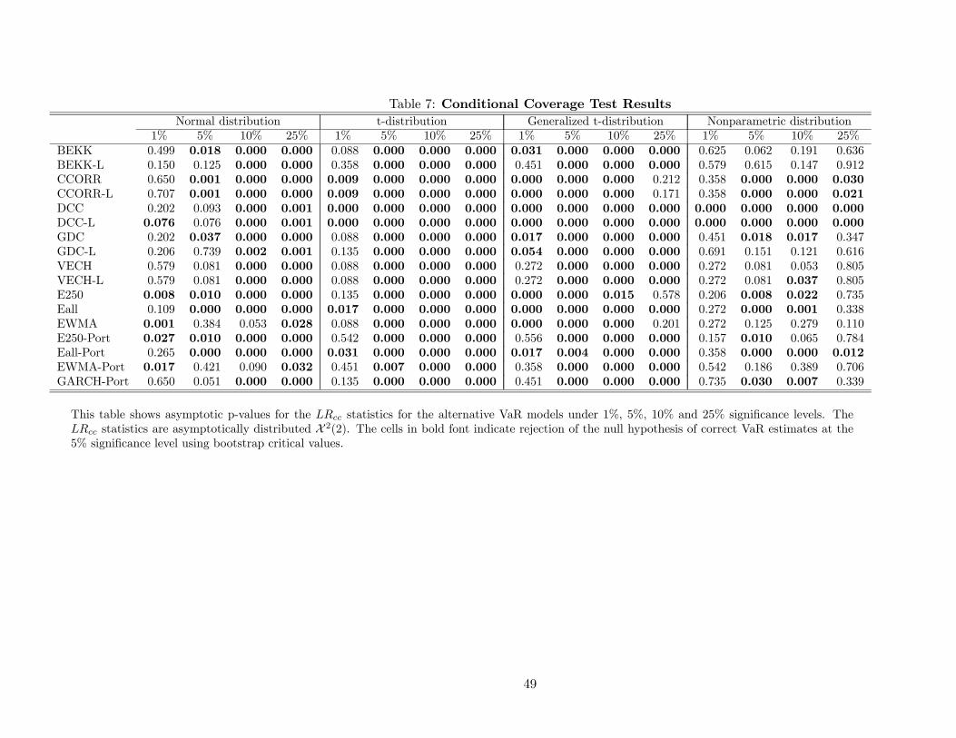
Table 7: Conditional Coverage Test ResultsNormal distribution t-distribution Generalized t-distribution Nonparametric distribution

1% 5% 10% 25% 1% 5% 10% 25% 1% 5% 10% 25% 1% 5% 10% 25%BEKK 0.499 0.018 0.000 0.000 0.088 0.000 0.000 0.000 0.031 0.000 0.000 0.000 0.625 0.062 0.191 0.636BEKK-L 0.150 0.125 0.000 0.000 0.358 0.000 0.000 0.000 0.451 0.000 0.000 0.000 0.579 0.615 0.147 0.912CCORR 0.650 0.001 0.000 0.000 0.009 0.000 0.000 0.000 0.000 0.000 0.000 0.212 0.358 0.000 0.000 0.030CCORR-L 0.707 0.001 0.000 0.000 0.009 0.000 0.000 0.000 0.000 0.000 0.000 0.171 0.358 0.000 0.000 0.021DCC 0.202 0.093 0.000 0.001 0.000 0.000 0.000 0.000 0.000 0.000 0.000 0.000 0.000 0.000 0.000 0.000DCC-L 0.076 0.076 0.000 0.001 0.000 0.000 0.000 0.000 0.000 0.000 0.000 0.000 0.000 0.000 0.000 0.000GDC 0.202 0.037 0.000 0.000 0.088 0.000 0.000 0.000 0.017 0.000 0.000 0.000 0.451 0.018 0.017 0.347GDC-L 0.206 0.739 0.002 0.001 0.135 0.000 0.000 0.000 0.054 0.000 0.000 0.000 0.691 0.151 0.121 0.616VECH 0.579 0.081 0.000 0.000 0.088 0.000 0.000 0.000 0.272 0.000 0.000 0.000 0.272 0.081 0.053 0.805VECH-L 0.579 0.081 0.000 0.000 0.088 0.000 0.000 0.000 0.272 0.000 0.000 0.000 0.272 0.081 0.037 0.805E250 0.008 0.010 0.000 0.000 0.135 0.000 0.000 0.000 0.000 0.000 0.015 0.578 0.206 0.008 0.022 0.735Eall 0.109 0.000 0.000 0.000 0.017 0.000 0.000 0.000 0.000 0.000 0.000 0.000 0.272 0.000 0.001 0.338EWMA 0.001 0.384 0.053 0.028 0.088 0.000 0.000 0.000 0.000 0.000 0.000 0.201 0.272 0.125 0.279 0.110E250-Port 0.027 0.010 0.000 0.000 0.542 0.000 0.000 0.000 0.556 0.000 0.000 0.000 0.157 0.010 0.065 0.784Eall-Port 0.265 0.000 0.000 0.000 0.031 0.000 0.000 0.000 0.017 0.004 0.000 0.000 0.358 0.000 0.000 0.012EWMA-Port 0.017 0.421 0.090 0.032 0.451 0.007 0.000 0.000 0.358 0.000 0.000 0.000 0.542 0.186 0.389 0.706GARCH-Port 0.650 0.051 0.000 0.000 0.135 0.000 0.000 0.000 0.451 0.000 0.000 0.000 0.735 0.030 0.007 0.339

This table shows asymptotic p-values for the LRcc statistics for the alternative VaR models under 1%, 5%, 10% and 25% significance levels. TheLRcc statistics are asymptotically distributed X 2(2). The cells in bold font indicate rejection of the null hypothesis of correct VaR estimates at the5% significance level using bootstrap critical values.

49

Table 8: Dynamic Quantile Test ResultsNormal distribution t-distribution Generalized t-distribution Nonparametric distribution

1% 5% 10% 25% 1% 5% 10% 25% 1% 5% 10% 25% 1% 5% 10% 25%BEKK 0.807 0.058 0.000 0.000 0.177 0.000 0.000 0.000 0.032 0.000 0.000 0.000 0.910 0.108 0.077 0.466BEKK-L 0.402 0.185 0.000 0.003 0.692 0.000 0.000 0.000 0.802 0.000 0.000 0.000 0.863 0.593 0.132 0.510CCOR 0.967 0.003 0.000 0.000 0.007 0.000 0.000 0.000 0.000 0.000 0.001 0.235 0.822 0.000 0.000 0.063CCOR-L 0.978 0.003 0.000 0.000 0.007 0.000 0.000 0.000 0.000 0.000 0.000 0.208 0.822 0.000 0.000 0.042DCC 0.752 0.146 0.001 0.007 0.000 0.000 0.000 0.000 0.000 0.000 0.000 0.000 0.000 0.000 0.000 0.000DCC-L 0.629 0.103 0.000 0.009 0.000 0.000 0.000 0.000 0.000 0.000 0.000 0.000 0.000 0.000 0.000 0.000GDC 0.771 0.099 0.000 0.000 0.278 0.000 0.000 0.000 0.027 0.001 0.000 0.000 0.892 0.056 0.031 0.354GDC-L 0.725 0.940 0.000 0.012 0.436 0.000 0.000 0.001 0.154 0.000 0.000 0.000 0.958 0.474 0.115 0.517VECH 0.960 0.104 0.000 0.000 0.283 0.000 0.000 0.000 0.718 0.000 0.000 0.000 0.718 0.104 0.193 0.409VECH-L 0.960 0.175 0.000 0.000 0.283 0.000 0.000 0.000 0.718 0.000 0.000 0.000 0.718 0.175 0.135 0.410E250 0.017 0.000 0.000 0.000 0.145 0.000 0.000 0.000 0.000 0.000 0.000 0.004 0.438 0.000 0.000 0.014Eall 0.213 0.000 0.000 0.000 0.042 0.000 0.000 0.000 0.000 0.000 0.000 0.000 0.383 0.000 0.000 0.333EWMA 0.043 0.104 0.018 0.021 0.173 0.000 0.000 0.000 0.000 0.000 0.000 0.132 0.516 0.013 0.035 0.024E250-Port 0.035 0.000 0.000 0.000 0.832 0.000 0.000 0.000 0.356 0.000 0.000 0.000 0.367 0.000 0.001 0.042Eall-Port 0.140 0.000 0.000 0.000 0.066 0.000 0.000 0.000 0.027 0.000 0.000 0.001 0.486 0.000 0.000 0.059EWMA-Port 0.053 0.120 0.023 0.023 0.597 0.000 0.000 0.000 0.528 0.000 0.000 0.000 0.772 0.019 0.044 0.135GARCH-Port 0.972 0.055 0.000 0.000 0.386 0.000 0.000 0.000 0.858 0.000 0.000 0.000 0.975 0.054 0.026 0.368

This table shows asymptotic p-values for the DQ statistic for the alternative VaR models under 1%, 5%, 10% and 25% signficance levels. The DQstatistics are asymptotically distributed X 2(7). The cells in bold font indicate rejection of the null hypothesis of correct VaR estimates at the 5%significance level using bootstrap critical values.

50

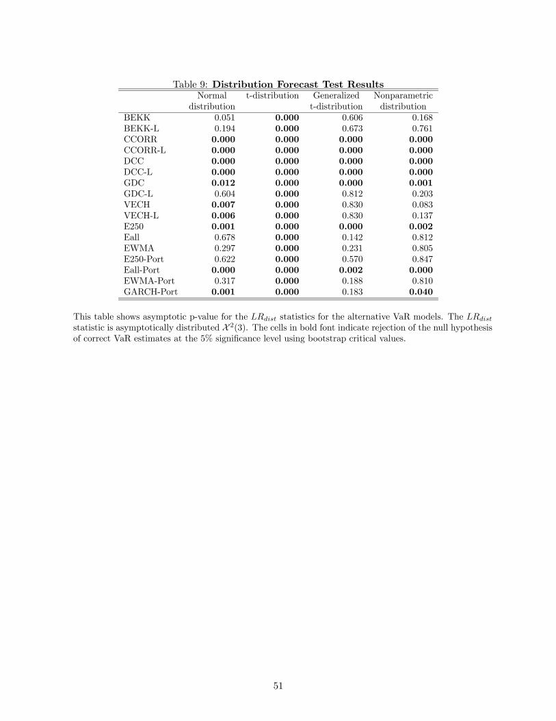
Table 9: Distribution Forecast Test ResultsNormal t-distribution Generalized Nonparametric

distribution t-distribution distributionBEKK 0.051 0.000 0.606 0.168BEKK-L 0.194 0.000 0.673 0.761CCORR 0.000 0.000 0.000 0.000CCORR-L 0.000 0.000 0.000 0.000DCC 0.000 0.000 0.000 0.000DCC-L 0.000 0.000 0.000 0.000GDC 0.012 0.000 0.000 0.001GDC-L 0.604 0.000 0.812 0.203VECH 0.007 0.000 0.830 0.083VECH-L 0.006 0.000 0.830 0.137E250 0.001 0.000 0.000 0.002Eall 0.678 0.000 0.142 0.812EWMA 0.297 0.000 0.231 0.805E250-Port 0.622 0.000 0.570 0.847Eall-Port 0.000 0.000 0.002 0.000EWMA-Port 0.317 0.000 0.188 0.810GARCH-Port 0.001 0.000 0.183 0.040

This table shows asymptotic p-value for the LRdist statistics for the alternative VaR models. The LRdiststatistic is asymptotically distributed X 2(3). The cells in bold font indicate rejection of the null hypothesisof correct VaR estimates at the 5% significance level using bootstrap critical values.

51

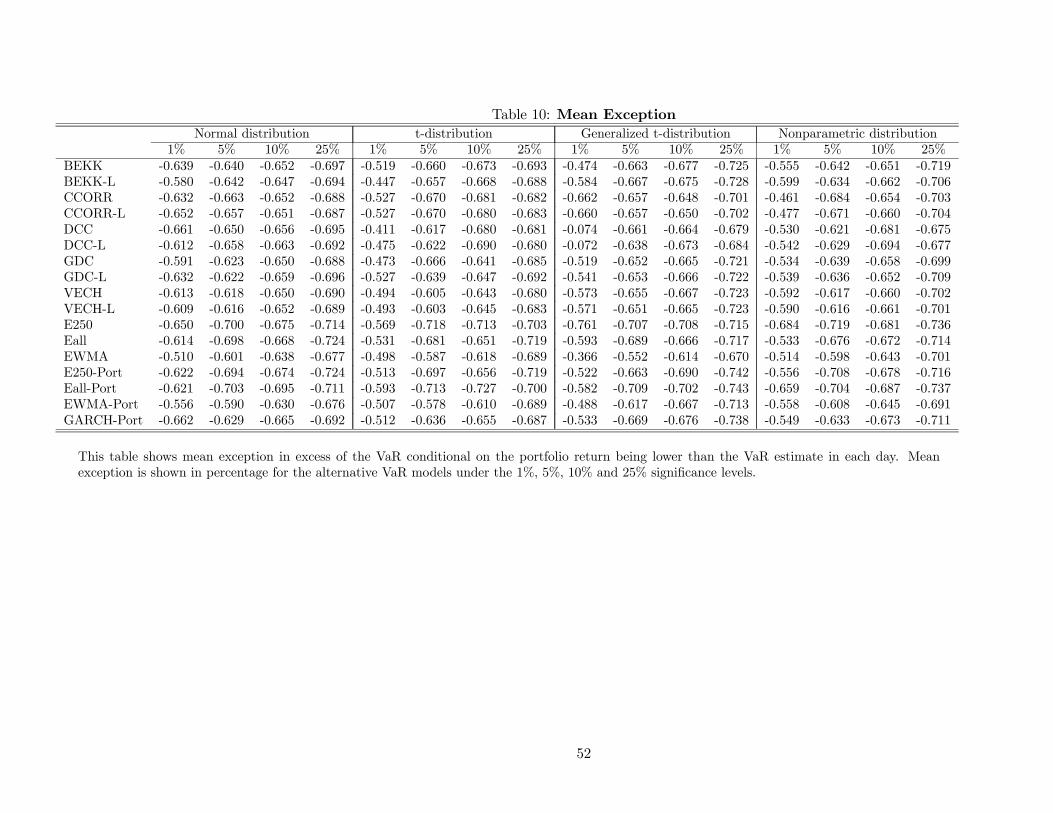
Table 10: Mean ExceptionNormal distribution t-distribution Generalized t-distribution Nonparametric distribution

1% 5% 10% 25% 1% 5% 10% 25% 1% 5% 10% 25% 1% 5% 10% 25%BEKK -0.639 -0.640 -0.652 -0.697 -0.519 -0.660 -0.673 -0.693 -0.474 -0.663 -0.677 -0.725 -0.555 -0.642 -0.651 -0.719BEKK-L -0.580 -0.642 -0.647 -0.694 -0.447 -0.657 -0.668 -0.688 -0.584 -0.667 -0.675 -0.728 -0.599 -0.634 -0.662 -0.706CCORR -0.632 -0.663 -0.652 -0.688 -0.527 -0.670 -0.681 -0.682 -0.662 -0.657 -0.648 -0.701 -0.461 -0.684 -0.654 -0.703CCORR-L -0.652 -0.657 -0.651 -0.687 -0.527 -0.670 -0.680 -0.683 -0.660 -0.657 -0.650 -0.702 -0.477 -0.671 -0.660 -0.704DCC -0.661 -0.650 -0.656 -0.695 -0.411 -0.617 -0.680 -0.681 -0.074 -0.661 -0.664 -0.679 -0.530 -0.621 -0.681 -0.675DCC-L -0.612 -0.658 -0.663 -0.692 -0.475 -0.622 -0.690 -0.680 -0.072 -0.638 -0.673 -0.684 -0.542 -0.629 -0.694 -0.677GDC -0.591 -0.623 -0.650 -0.688 -0.473 -0.666 -0.641 -0.685 -0.519 -0.652 -0.665 -0.721 -0.534 -0.639 -0.658 -0.699GDC-L -0.632 -0.622 -0.659 -0.696 -0.527 -0.639 -0.647 -0.692 -0.541 -0.653 -0.666 -0.722 -0.539 -0.636 -0.652 -0.709VECH -0.613 -0.618 -0.650 -0.690 -0.494 -0.605 -0.643 -0.680 -0.573 -0.655 -0.667 -0.723 -0.592 -0.617 -0.660 -0.702VECH-L -0.609 -0.616 -0.652 -0.689 -0.493 -0.603 -0.645 -0.683 -0.571 -0.651 -0.665 -0.723 -0.590 -0.616 -0.661 -0.701E250 -0.650 -0.700 -0.675 -0.714 -0.569 -0.718 -0.713 -0.703 -0.761 -0.707 -0.708 -0.715 -0.684 -0.719 -0.681 -0.736Eall -0.614 -0.698 -0.668 -0.724 -0.531 -0.681 -0.651 -0.719 -0.593 -0.689 -0.666 -0.717 -0.533 -0.676 -0.672 -0.714EWMA -0.510 -0.601 -0.638 -0.677 -0.498 -0.587 -0.618 -0.689 -0.366 -0.552 -0.614 -0.670 -0.514 -0.598 -0.643 -0.701E250-Port -0.622 -0.694 -0.674 -0.724 -0.513 -0.697 -0.656 -0.719 -0.522 -0.663 -0.690 -0.742 -0.556 -0.708 -0.678 -0.716Eall-Port -0.621 -0.703 -0.695 -0.711 -0.593 -0.713 -0.727 -0.700 -0.582 -0.709 -0.702 -0.743 -0.659 -0.704 -0.687 -0.737EWMA-Port -0.556 -0.590 -0.630 -0.676 -0.507 -0.578 -0.610 -0.689 -0.488 -0.617 -0.667 -0.713 -0.558 -0.608 -0.645 -0.691GARCH-Port -0.662 -0.629 -0.665 -0.692 -0.512 -0.636 -0.655 -0.687 -0.533 -0.669 -0.676 -0.738 -0.549 -0.633 -0.673 -0.711

This table shows mean exception in excess of the VaR conditional on the portfolio return being lower than the VaR estimate in each day. Meanexception is shown in percentage for the alternative VaR models under the 1%, 5%, 10% and 25% significance levels.

52

Table 11: Normal Transform Test ResultsNormal distribution t-distribution Generalized t-distribution Nonparametric distribution

1% 5% 10% 25% 1% 5% 10% 25% 1% 5% 10% 25% 1% 5% 10% 25%BEKK 0.021 0.026 0.028 0.031 0.000 0.000 0.000 0.000 0.356 0.386 0.399 0.414 0.066 0.079 0.084 0.091BEKK-L 0.113 0.131 0.139 0.149 0.000 0.000 0.000 0.000 0.597 0.552 0.534 0.512 0.585 0.625 0.642 0.663CCORR 0.000 0.000 0.000 0.000 0.000 0.000 0.000 0.000 0.000 0.000 0.000 0.000 0.000 0.000 0.000 0.000CCORR-L 0.000 0.000 0.000 0.000 0.000 0.000 0.000 0.000 0.000 0.000 0.000 0.000 0.000 0.000 0.000 0.000DCC 0.000 0.000 0.000 0.000 0.000 0.000 0.000 0.000 0.000 0.000 0.000 0.000 0.000 0.000 0.000 0.000DCC-L 0.000 0.000 0.000 0.000 0.000 0.000 0.000 0.000 0.000 0.000 0.000 0.000 0.000 0.000 0.000 0.000GDC 0.004 0.006 0.006 0.007 0.000 0.000 0.000 0.000 0.000 0.000 0.000 0.000 0.000 0.000 0.000 0.000GDC-L 0.672 0.707 0.721 0.739 0.000 0.000 0.000 0.000 0.765 0.737 0.726 0.711 0.095 0.111 0.118 0.128VECH 0.003 0.004 0.005 0.005 0.000 0.000 0.000 0.000 0.815 0.811 0.808 0.804 0.034 0.041 0.044 0.049VECH-L 0.003 0.004 0.004 0.005 0.000 0.000 0.000 0.000 0.808 0.806 0.804 0.801 0.064 0.076 0.081 0.088E250 0.000 0.000 0.000 0.000 0.000 0.000 0.000 0.000 0.000 0.000 0.000 0.000 0.000 0.000 0.001 0.001Eall 0.492 0.530 0.547 0.567 0.000 0.000 0.000 0.000 0.046 0.055 0.059 0.064 0.730 0.691 0.676 0.659EWMA 0.563 0.515 0.496 0.473 0.000 0.000 0.000 0.000 0.116 0.132 0.138 0.147 1.000 1.000 1.000 1.000E250-Port 0.421 0.458 0.473 0.493 0.000 0.000 0.000 0.000 0.462 0.420 0.403 0.383 0.770 0.734 0.720 0.703Eall-Port 0.000 0.000 0.000 0.000 0.000 0.000 0.000 0.000 0.000 0.000 0.000 0.001 0.000 0.000 0.000 0.000EWMA-Port 0.591 0.541 0.522 0.499 0.000 0.000 0.000 0.000 0.170 0.148 0.139 0.130 1.000 1.000 1.000 1.000GARCH-Port 0.000 0.001 0.001 0.001 0.000 0.000 0.000 0.000 0.075 0.087 0.092 0.099 0.014 0.018 0.019 0.021

This table shows the p-value for the LRmag test statistic for the alternative VaR models under 1%, 5%, 10% and 25% significance levels. The LRmagstatistic is asymptotically distributed X 2(2). The cells in bold font indicate rejection of the null hypothesis of correct VaR estimates at the 5%significance level using bootstrap critical values.

53

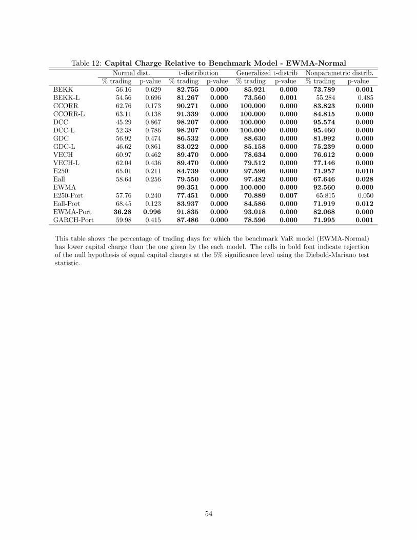
Table 12: Capital Charge Relative to Benchmark Model - EWMA-NormalNormal dist. t-distribution Generalized t-distrib Nonparametric distrib.

% trading p-value % trading p-value % trading p-value % trading p-valueBEKK 56.16 0.629 82.755 0.000 85.921 0.000 73.789 0.001BEKK-L 54.56 0.696 81.267 0.000 73.560 0.001 55.284 0.485CCORR 62.76 0.173 90.271 0.000 100.000 0.000 83.823 0.000CCORR-L 63.11 0.138 91.339 0.000 100.000 0.000 84.815 0.000DCC 45.29 0.867 98.207 0.000 100.000 0.000 95.574 0.000DCC-L 52.38 0.786 98.207 0.000 100.000 0.000 95.460 0.000GDC 56.92 0.474 86.532 0.000 88.630 0.000 81.992 0.000GDC-L 46.62 0.861 83.022 0.000 85.158 0.000 75.239 0.000VECH 60.97 0.462 89.470 0.000 78.634 0.000 76.612 0.000VECH-L 62.04 0.436 89.470 0.000 79.512 0.000 77.146 0.000E250 65.01 0.211 84.739 0.000 97.596 0.000 71.957 0.010Eall 58.64 0.256 79.550 0.000 97.482 0.000 67.646 0.028EWMA - - 99.351 0.000 100.000 0.000 92.560 0.000E250-Port 57.76 0.240 77.451 0.000 70.889 0.007 65.815 0.050Eall-Port 68.45 0.123 83.937 0.000 84.586 0.000 71.919 0.012EWMA-Port 36.28 0.996 91.835 0.000 93.018 0.000 82.068 0.000GARCH-Port 59.98 0.415 87.486 0.000 78.596 0.000 71.995 0.001

This table shows the percentage of trading days for which the benchmark VaR model (EWMA-Normal)has lower capital charge than the one given by the each model. The cells in bold font indicate rejectionof the null hypothesis of equal capital charges at the 5% significance level using the Diebold-Mariano teststatistic.

54

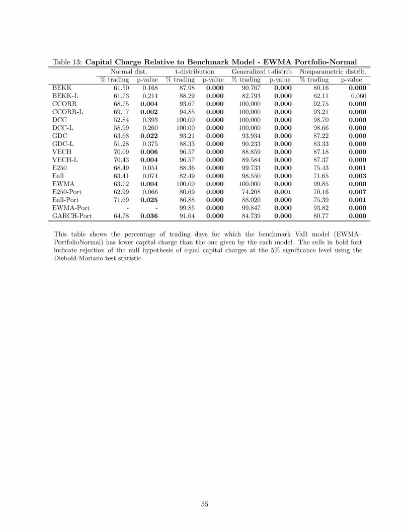
Table 13: Capital Charge Relative to Benchmark Model - EWMA Portfolio-NormalNormal dist. t-distribution Generalized t-distrib Nonparametric distrib.

% trading p-value % trading p-value % trading p-value % trading p-valueBEKK 61.50 0.168 87.98 0.000 90.767 0.000 80.16 0.000BEKK-L 61.73 0.214 88.29 0.000 82.793 0.000 62.11 0.060CCORR 68.75 0.004 93.67 0.000 100.000 0.000 92.75 0.000CCORR-L 69.17 0.002 94.85 0.000 100.000 0.000 93.21 0.000DCC 52.84 0.393 100.00 0.000 100.000 0.000 98.70 0.000DCC-L 58.99 0.260 100.00 0.000 100.000 0.000 98.66 0.000GDC 63.68 0.022 93.21 0.000 93.934 0.000 87.22 0.000GDC-L 51.28 0.375 88.33 0.000 90.233 0.000 83.33 0.000VECH 70.09 0.006 96.57 0.000 88.859 0.000 87.18 0.000VECH-L 70.43 0.004 96.57 0.000 89.584 0.000 87.37 0.000E250 68.49 0.054 88.36 0.000 99.733 0.000 75.43 0.001Eall 63.41 0.074 82.49 0.000 98.550 0.000 71.65 0.003EWMA 63.72 0.004 100.00 0.000 100.000 0.000 99.85 0.000E250-Port 62.99 0.066 80.69 0.000 74.208 0.001 70.16 0.007Eall-Port 71.69 0.025 86.88 0.000 88.020 0.000 75.39 0.001EWMA-Port - - 99.85 0.000 99.847 0.000 93.82 0.000GARCH-Port 64.78 0.036 91.64 0.000 84.739 0.000 80.77 0.000

This table shows the percentage of trading days for which the benchmark VaR model (EWMA—PortfolioNormal) has lower capital charge than the one given by the each model. The cells in bold fontindicate rejection of the null hypothesis of equal capital charges at the 5% significance level using theDiebold-Mariano test statistic.

55

Figure 1: Time Series of Interest and Foreign Exchange RatesPanel A.1: US$ 3-month Interest Rate

0

4

8

12

16

20

24

28

32

79 80 81 82 83 84 85 86 87 88 89 90 91 92 93 94 95 96 97 98 99 00

percentage

-10

-8

-6

-4

-2

0

2

percentage

Panel A.2: DM 3-month Interest Rate

0

2

4

6

8

10

12

14

16

18

20

22

79 80 81 82 83 84 85 86 87 88 89 90 91 92 93 94 95 96 97 98 99 00

percentage

-4

-3

-2

-1

0

1

2

percentage

Panel A.3: JY 3-month Interest Rate

0

2

4

6

8

10

12

14

16

18

20

22

24

26

79 80 81 82 83 84 85 86 87 88 89 90 91 92 93 94 95 96 97 98 99 00

percentage

-7

-6

-5

-4

-3

-2

-1

0

1

2

3

percentage

Panel A.4: DM/US$ Exchange Rates

1.25

1.5

1.75

2

2.25

2.5

2.75

3

3.25

3.5

3.75

4

79 80 81 82 83 84 85 86 87 88 89 90 91 92 93 94 95 96 97 98 99 00-16

-14

-12

-10

-8

-6

-4

-2

0

2

4

percentage

Panel A.5: JY/US$ Exchange Rates

50

100

150

200

250

300

350

400

79 80 81 82 83 84 85 86 87 88 89 90 91 92 93 94 95 96 97 98 99 00-20

-15

-10

-5

0

5

percentage

Panel A.6: Portfolio Return

-6

-4

-2

0

2

4

6

8

10

79 80 81 82 83 84 85 86 87 88 89 90 91 92 93 94 95 96 97 98 99 00

The figure plots the daily time series of interest rate and foreign exchange rate levels (black line) andinterest rate first differences, foreign exchange rate geometric returns, and portfolio returns (grey line) forthe sample period between January 12, 1979 and December 29, 2000.

56