Journal of Hydrology 493 (2013) 105–114

Contents lists available at SciVerse ScienceDirect

Journal of Hydrology

journal homepage: www.elsevier .com/ locate / jhydrol

Evaluating geostatistical methods of blending satellite and gauge datato estimate near real-time daily rainfall for Australia

0022-1694/$ - see front matter � 2013 Elsevier B.V. All rights reserved.http://dx.doi.org/10.1016/j.jhydrol.2013.04.024

⇑ Corresponding author. Tel.: +61 2 6246 5925; fax: +61 2 6246 5965.E-mail address: adrian.chappell@csiro.au (A. Chappell).

1 Present address: Environmental Remote Sensing Laboratory (LTE), École Poly-technique Fédérale de Lausanne (EPFL), GR C2 564, 1015 Lausanne, Switzerland.

Adrian Chappell a,1,⇑, Luigi J. Renzullo a, Tim H. Raupach a, Malcolm Haylock b

a CSIRO Land and Water, GPO Box 1666, Canberra, ACT 2601, Australiab Partner Reinsurance Company, Zurich, Switzerland

a r t i c l e i n f o s u m m a r y

Article history:Received 30 August 2012Received in revised form 14 January 2013Accepted 13 April 2013Available online 24 April 2013This manuscript was handled byKonstantine P. Georgakakos, Editor-in-Chief,with the assistance of Hervé Andrieu,Associate Editor

Keywords:GaugeSatellitePrecipitationGeostatisticsCokrigingRainfall intermittency

Rain gauges provide valuable information about the amount and frequency of rainfall. In Australia, themajority of rain gauges are located in populated, wet coastal regions. Approximately 2000 gauges report-ing within 24 h of a target day were used to make near real-time (NRT) estimates of daily precipitation.The remaining �4000 gauges for the same target day were used to evaluate bias and estimation perfor-mance using several traditional statistics. There is considerable potential to improve the estimation ofrainfall in Australia using related ancillary data, particularly in sparsely gauged areas. The Tropical Rain-fall Measuring Mission (TRMM) Multisatellite Precipitation Analysis (TMPA-RT) near real-time product(3B42RT) provided images (0.25� resolution) of precipitation across Australia. Daily precipitation wasestimated in 2009/10 approximately every 5 km across Australia. This study evaluated selected geosta-tistical methods for estimating daily rainfall maps across Australia. It tackled the change of support prob-lem and spatial intermittency of daily rainfall data in blending satellite and gauge data. Dissensionoccurred amongst traditional global statistical measures of performance which were compounded byextremes of gauge density. Overall, our assessment is that blending the 3B42RT satellite and rain gaugedata was not worthwhile. However, the blending considerably reduced the estimation variance indicatingthat uncertainty of the map estimates was a neglected property necessary to detect change and differencein patterns.

� 2013 Elsevier B.V. All rights reserved.

1. Introduction

Knowledge of the amount, spatial distribution and temporalvariation of daily precipitation is essential for provision of publicinformation, hydrological modelling and flood forecasting, climatemonitoring and climate model validation. Rain gauges providevaluable information about the amount and frequency of rainfall.However, they are commonly located in, or near to, populationcentres to provide timely information for water resource manage-ment. Automated weather stations including rain gauges are tooexpensive to form a dense network of measurements. In Australia,the majority of rain gauges are located in populated, wetter coast-al regions and relatively few stations are located in drier, inlandregions. Areas of high rain gauge density provide more reliableestimates at unsampled locations than areas of low rain gaugedensity.

The estimation of the spatial distribution of rainfall can be im-proved with the inclusion of ancillary data (radar, satellite and/or

topography) that is related to the rainfall. For example, Krajewski(1987) found improved estimates when blending rain gauge andradar information with bias. Notably, he found little improvementin the blending when the bias in the radar data was removed.Goovaerts (2000) augmented monthly rainfall totals for Portugalwith digital elevation data. Velasco-Forero et al. (2009) showedthat radar data considerably improved the estimation of hourlyrainfall in Catalonia, Spain. Although weather radar is very usefulfor augmenting rainfall estimation, radar networks in Australiaare limited to the coastal regions. Satellite-based estimates providesynoptic images of the spatial distribution of precipitation eventsat 0.5–3 h intervals, at between 0.07� and 0.25� resolution (Joyceet al., 2004; Kubota et al., 2007; Huffman et al., 2007). While theabsolute accuracy of satellite rainfall products is questionable (Tianand Peters-Lidard, 2011) and remains the subject of on-goingworldwide assessment (Ebert et al., 2007; IPWG, 2011), they nev-ertheless provide unique information on the spatial extent of therainfall, particularly for those regions of the Australian continentwhere the network of rain gauges is sparse. It is only relatively re-cently that the statistical blending of satellite-derived precipitationproducts and rain gauge measurements has been explored to gen-erate fine-resolution rainfall estimates at continental scales (Vilaet al., 2009; Li and Shao, 2010; Clarke et al., 2011).

106 A. Chappell et al. / Journal of Hydrology 493 (2013) 105–114

There remain two key issues with the blending of daily raingauge measurements and satellite data: (i) the change of supportproblem (COSP) and (ii) spatial intermittency of daily rainfall data.There is a considerable difference in the resolution of informationwith satellite data providing either radiance measurements orrainfall estimates over a large pixel (0.25� � 0.25�) whilst raingauge observations represent such a small area they may reason-ably be considered to be a point. Any blending of these differentsources of data should adequately account for these differences.The support of a sample has come to mean simply the volume ofa datum. The COSP is how the spatial variation in one variableassociated with a given support relates to that of another variablewith a different support (e.g., Gotway and Young, 2002; Kyriakidis,2004). Spatial intermittency is related to the delivery of daily rain-fall in discrete patches in space and time. This causes a discontin-uous surface of rainfall i.e., areas of zero rainfall between areas ofnon-zero rainfall (Creutin and Obled, 1982). Spatial intermittencyundermines the common assumption of continuity in the geosta-tistical treatment of the data. However, Barancourt et al. (1992)showed that a straightforward method to tackling this mixed dis-tribution is to threshold the rainfall distribution with an indicatortransform, map the presence and absence of rainfall, and combineit with a wet area map.

This study is an evaluation of geostatistical techniques for blend-ing satellite and gauge data to estimate daily rainfall maps acrossAustralia. Only geostatistical techniques will be considered basedon the premise that rainfall estimates of these techniques give moreaccurate results than methods of interpolation (Grimes and Pardo-Igúzquiza, 2010; Hofstra et al., 2008). Many studies (e.g., Creutinand Obled, 1982; Lebel et al., 1987; Goovaerts, 2000) have used geo-statistics to estimate rainfall. Kriging is the central tool for geosta-tistics and our experiments will be conducted using only kriging-based techniques. The aim of this paper is to demonstrate the im-pact of upscaling and rainfall intermittency on the blending of sa-tellite data with rain gauge observations for the spatial estimationof daily rainfall. Point estimates of daily rainfall are made at 5 kmintervals across Australia every day for an intensive observationperiod (IOP) between 31 May 2009 and 31 May 2010. To achievethe aim, we have two objectives and employ several estimationtechniques. The first objective is to explicitly tackle the COSP de-fined above. We use block-kriging to make rainfall estimates withthe same support as the satellite data and develop an appropriatecross-variogram before using cokriging and the gauge data to makethe maps. The second objective is to consider the impact of (inap-propriately) assuming continuity in daily rainfall which may beintermittent over space. The two-stage process of Barancourtet al. (1992) is used with the techniques described previously to ac-count for the COSP. We compare these estimation techniques withordinary point kriging by employing several validation metrics toisolate the benefits of the satellite data and to determine how bestto blend the satellite data. The local estimation variance maps dem-onstrate the impact of the number and configuration of rain gaugeinformation and consequently provide a rudimentary measure of atechnique’s relative uncertainty.

2. Precipitation data

2.1. Australian rain gauge networks

Daily gauge data used in our investigations covering the period31 May 2009 – 31 May 2010 were obtained from the data holdingsof the Australian Bureau of Meteorology (BoM). No additional qual-ity checks were performed on these data. The observations areinterpreted as the 24-h accumulated rainfall to 9 am (local time)on the day of interest. The data include the measurements fromthe network of gauges reporting in near real-time (NRT) i.e., within

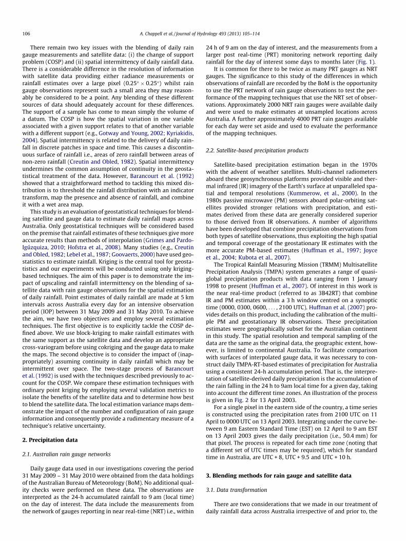
24 h of 9 am on the day of interest, and the measurements from alarger post real-time (PRT) monitoring network reporting dailyrainfall for the day of interest some days to months later (Fig. 1).

It is common for there to be twice as many PRT gauges as NRTgauges. The significance to this study of the differences in whichobservations of rainfall are recorded by the BoM is the opportunityto use the PRT network of rain gauge observations to test the per-formance of the mapping techniques that use the NRT set of obser-vations. Approximately 2000 NRT rain gauges were available dailyand were used to make estimates at unsampled locations acrossAustralia. A further approximately 4000 PRT rain gauges availablefor each day were set aside and used to evaluate the performanceof the mapping techniques.

2.2. Satellite-based precipitation products

Satellite-based precipitation estimation began in the 1970swith the advent of weather satellites. Multi-channel radiometersaboard these geosynchronous platforms provided visible and ther-mal infrared (IR) imagery of the Earth’s surface at unparalleled spa-tial and temporal resolutions (Kummerow, et al., 2000). In the1980s passive microwave (PM) sensors aboard polar-orbiting sat-ellites provided stronger relations with precipitation, and esti-mates derived from these data are generally considered superiorto those derived from IR observations. A number of algorithmshave been developed that combine precipitation observations fromboth types of satellite observations, thus exploiting the high spatialand temporal coverage of the geostationary IR estimates with themore accurate PM-based estimates (Huffman et al., 1997; Joyceet al., 2004; Kubota et al., 2007).

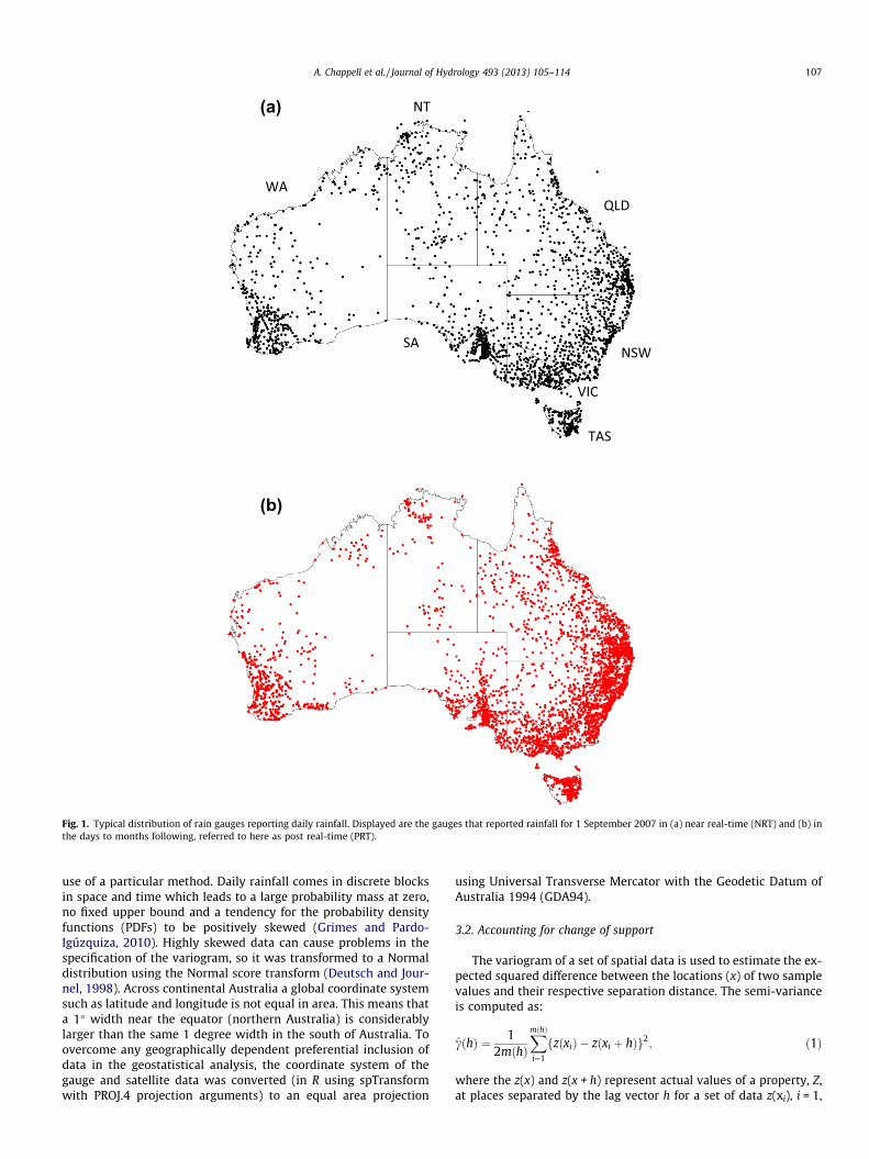
The Tropical Rainfall Measuring Mission (TRMM) MultisatellitePrecipitation Analysis (TMPA) system generates a range of quasi-global precipitation products with data ranging from 1 January1998 to present (Huffman et al., 2007). Of interest in this work isthe near real-time product (referred to as 3B42RT) that combineIR and PM estimates within a 3 h window centred on a synoptictime (0000, 0300, 0600, . . . , 2100 UTC). Huffman et al. (2007) pro-vides details on this product, including the calibration of the multi-ple PM and geostationary IR observations. These precipitationestimates were geographically subset for the Australian continentin this study. The spatial resolution and temporal sampling of thedata are the same as the original data, the geographic extent, how-ever, is limited to continental Australia. To facilitate comparisonwith surfaces of interpolated gauge data, it was necessary to con-struct daily TMPA-RT-based estimates of precipitation for Australiausing a consistent 24-h accumulation period. That is, the interpre-tation of satellite-derived daily precipitation is the accumulation ofthe rain falling in the 24 h to 9am local time for a given day, takinginto account the different time zones. An illustration of the processis given in Fig. 2 for 13 April 2003.

For a single pixel in the eastern side of the country, a time seriesis constructed using the precipitation rates from 2100 UTC on 11April to 0000 UTC on 13 April 2003. Integrating under the curve be-tween 9 am Eastern Standard Time (EST) on 12 April to 9 am ESTon 13 April 2003 gives the daily precipitation (i.e., 50.4 mm) forthat pixel. The process is repeated for each time zone (noting thata different set of UTC times may be required), which for standardtime in Australia, are UTC + 8, UTC + 9.5 and UTC + 10 h.

3. Blending methods for rain gauge and satellite data

3.1. Data transformation

There are two considerations that we made in our treatment ofdaily rainfall data across Australia irrespective of and prior to, the

(a)

(b)

Fig. 1. Typical distribution of rain gauges reporting daily rainfall. Displayed are the gauges that reported rainfall for 1 September 2007 in (a) near real-time (NRT) and (b) inthe days to months following, referred to here as post real-time (PRT).

A. Chappell et al. / Journal of Hydrology 493 (2013) 105–114 107

use of a particular method. Daily rainfall comes in discrete blocksin space and time which leads to a large probability mass at zero,no fixed upper bound and a tendency for the probability densityfunctions (PDFs) to be positively skewed (Grimes and Pardo-Igúzquiza, 2010). Highly skewed data can cause problems in thespecification of the variogram, so it was transformed to a Normaldistribution using the Normal score transform (Deutsch and Jour-nel, 1998). Across continental Australia a global coordinate systemsuch as latitude and longitude is not equal in area. This means thata 1� width near the equator (northern Australia) is considerablylarger than the same 1 degree width in the south of Australia. Toovercome any geographically dependent preferential inclusion ofdata in the geostatistical analysis, the coordinate system of thegauge and satellite data was converted (in R using spTransformwith PROJ.4 projection arguments) to an equal area projection

using Universal Transverse Mercator with the Geodetic Datum ofAustralia 1994 (GDA94).

3.2. Accounting for change of support

The variogram of a set of spatial data is used to estimate the ex-pected squared difference between the locations (x) of two samplevalues and their respective separation distance. The semi-varianceis computed as:

cðhÞ ¼ 12mðhÞ

XmðhÞ

i¼1

fzðxiÞ � zðxi þ hÞg2; ð1Þ

where the z(x) and z(x + h) represent actual values of a property, Z,at places separated by the lag vector h for a set of data z(xi), i = 1,

(a)

(b)

Fig. 2. Graphical depiction of the approach used to construct daily satellite-based precipitation estimates for Australia for 13 April 2003: (a) for a single pixel, using all theprecipitation rates in the 24 h to 9 am Eastern Standard Time (EST), and (b) for the whole continent, taking into account the three different time zones.

108 A. Chappell et al. / Journal of Hydrology 493 (2013) 105–114

2, . . ., m(h), where m(h) is the number of pairs of data points. Thevariogram summarises the spatial variation in a property and de-scribes how that variation changes with increasing separation dis-tance between samples. Once the variogram has been calculatedit is fitted with an ‘‘authorised’’ model selected from several fami-lies of models (e.g., Gaussian, spherical, exponential) and a nuggetterm, if appropriate, which ensure validity of the model when mak-ing estimates at unsampled locations.

Remote sensing data provides a valuable secondary variable forblending with rain gauge (point) observations. However, the infor-mation available from 3B42RT is from a very large support (0.25�,�25 km square grid) whilst rain gauge observations represent sucha small support that they may be considered points. Any blendingof these different sources of data should take account of these dif-ferences in support. The variogram on one support can be relatedto that on another. For distances h which are very large in compar-ison with the dimension of support v, the regularized variogram isobtained from the point variogram by subtracting a constant termcðv ;vÞwhich is related to the dimensions and geometry of the sup-port v of the regularization (Journel and Huijbregts, 1978, p. 78)i.e., the dispersion variance of the support (Webster and Oliver,2001, p. 64). In this way, the variogram of the rain gauges can beregularized to the support of the satellite data. Since we also needto calculate the cross-variogram, we took a practical alternative tothis approach that has been adopted by others (e.g., Krajewski,1987; Chappell, 1998). Namely, we identified the NRT rain gaugesthat fell within satellite pixels and used block-kriging to estimate

rainfall over selected blocks that coincided with those satellite pix-els. This approach was used to tackle the COSP and these 0.25�square blocks (�25 km square) represented the upscaled NRTgauge data for use with cokriging. For each day of gauge and satel-lite data, variograms were calculated and fitted with a range ofmodels. The best model was selected using the sum of squares dif-ference between predictions and measurements. This automatedprocess ensured that a bespoke spatial model was available foreach day. Selected experimental variograms showed no evidencethat spatial variation was dependent on direction (anisotropic).Consequently, we assumed that the variogram was isotropic andfitted a model on that basis for every day of gauge and satellitedata.

3.3. Kriging and cokriging

Kriging is the method of geostatistical estimation at unsampledlocations (points) or areas (blocks). It is one of the most reliabletwo-dimensional spatial estimators (Laslett et al., 1987; Laslettand McBratney, 1990; Laslett, 1994) and often produces more reli-able estimates than methods of interpolation (Webster and Oliver,2001). Using ordinary point kriging (PK) we estimated daily rainfallat unsampled locations on a 5 km square grid across Australia. Themap provided a baseline output against which to compare theother methods. The 5 km grid spacing used here was set for consis-tency and subsequent comparison with two extant national gauge-only rainfall products (Jeffrey et al., 2001; Jones et al., 2009).

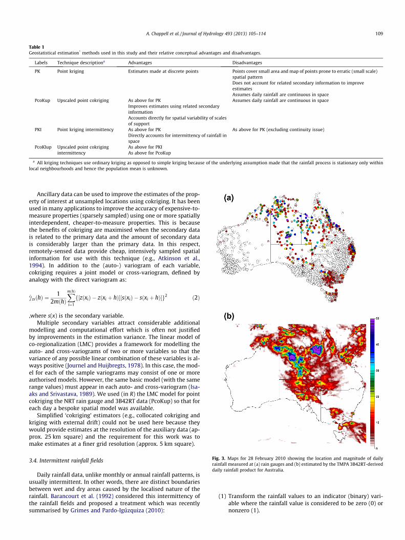
Table 1Geostatistical estimation* methods used in this study and their relative conceptual advantages and disadvantages.

Labels Technique descriptiona Advantages Disadvantages

PK Point kriging Estimates made at discrete points Points cover small area and map of points prone to erratic (small scale)spatial patternDoes not account for related secondary information to improveestimatesAssumes daily rainfall are continuous in space

PcoKup Upscaled point cokriging As above for PK Assumes daily rainfall are continuous in spaceImproves estimates using related secondaryinformationAccounts directly for spatial variability of scalesof support

PKI Point kriging intermittency As above for PK As above for PK (excluding continuity issue)Directly accounts for intermittency of rainfall inspace

PcoKIup Upscaled point cokrigingintermittency

As above for PKIAs above for PcoKup

a All kriging techniques use ordinary kriging as opposed to simple kriging because of the underlying assumption made that the rainfall process is stationary only withinlocal neighbourhoods and hence the population mean is unknown.

Fig. 3. Maps for 28 February 2010 showing the location and magnitude of dailyrainfall measured at (a) rain gauges and (b) estimated by the TMPA 3B42RT-deriveddaily rainfall product for Australia.

A. Chappell et al. / Journal of Hydrology 493 (2013) 105–114 109

Ancillary data can be used to improve the estimates of the prop-erty of interest at unsampled locations using cokriging. It has beenused in many applications to improve the accuracy of expensive-to-measure properties (sparsely sampled) using one or more spatiallyinterdependent, cheaper-to-measure properties. This is becausethe benefits of cokriging are maximised when the secondary datais related to the primary data and the amount of secondary datais considerably larger than the primary data. In this respect,remotely-sensed data provide cheap, intensively sampled spatialinformation for use with this technique (e.g., Atkinson et al.,1994). In addition to the (auto-) variogram of each variable,cokriging requires a joint model or cross-variogram, defined byanalogy with the direct variogram as:

czsðhÞ ¼1

2mðhÞXmðhÞ

i¼1

f½zðxiÞ � zðxi þ hÞ�½sðxiÞ � sðxi þ hÞ�g2 ð2Þ

,where s(x) is the secondary variable.Multiple secondary variables attract considerable additional

modelling and computational effort which is often not justifiedby improvements in the estimation variance. The linear model ofco-regionalization (LMC) provides a framework for modelling theauto- and cross-variograms of two or more variables so that thevariance of any possible linear combination of these variables is al-ways positive (Journel and Huijbregts, 1978). In this case, the mod-el for each of the sample variograms may consist of one or moreauthorised models. However, the same basic model (with the samerange values) must appear in each auto- and cross-variogram (Isa-aks and Srivastava, 1989). We used (in R) the LMC model for pointcokriging the NRT rain gauge and 3B42RT data (PcoKup) so that foreach day a bespoke spatial model was available.

Simplified ‘cokriging’ estimators (e.g., collocated cokriging andkriging with external drift) could not be used here because theywould provide estimates at the resolution of the auxiliary data (ap-prox. 25 km square) and the requirement for this work was tomake estimates at a finer grid resolution (approx. 5 km square).

3.4. Intermittent rainfall fields

Daily rainfall data, unlike monthly or annual rainfall patterns, isusually intermittent. In other words, there are distinct boundariesbetween wet and dry areas caused by the localised nature of therainfall. Barancourt et al. (1992) considered this intermittency ofthe rainfall fields and proposed a treatment which was recentlysummarised by Grimes and Pardo-Igúzquiza (2010):

(1) Transform the rainfall values to an indicator (binary) vari-able where the rainfall value is considered to be zero (0) ornonzero (1).

110 A. Chappell et al. / Journal of Hydrology 493 (2013) 105–114

(2) Calculate the experimental variogram of the indicator dataand fit a model in the manner described above (Section 3.1).

(3) Estimate the soft indicator field I(x) on a regular grid by(indicator) (co)kriging values between 0 and 1 which repre-sent the probability of rainfall occurrence.

(4) Produce a hard indicator field I ⁄ (x) by selecting a probabil-ity threshold T such that I ⁄ (x) = 1 for I(x) > T and I ⁄ (x) = 0for I(x) 6 T where T is set to ensure that the proportion ofthe target domain designated rainy is the same as thenumerical proportion of gauges registering nonzero rainfallamounts.

(5) Calculate and fit a model to the variogram of the nonzerorainfall values and estimate the rainfall amount field F(x)using ordinary (co)kriging.

(6) Estimate the final rainfall field Z(x) = I ⁄ (x)F(x).

We coded this algorithm (in R) and developed a workflow andrepeated it for each day of data and therefore had bespoke spatialmodels to implement this intermittent approach for ordinary pointkriging (PKI) for use as a baseline comparison. We also imple-mented this approach for point cokriging by accounting for thechange of support (PcoKIup). The techniques used in this studyare summarised in Table 1.

3.5. Evaluation statistics

In addition to making estimates on a regular grid we made esti-mates using the same kriging techniques at the locations of thepost real-time (PRT) rain gauges which are here used as an inde-pendent evaluation dataset (Section 2.1). The specific point esti-mates for each day between 31 May 2009 and 31 May 2010

Fig. 4. Maps of daily rainfall (mm) for 28 February 2010 at points on a �5 km regular gridwith upscaling (c) PcoKup and expecting intermittency by the point kriging estimators

were then compared with those PRT rain gauge values that wereset aside. Several nation-wide error statistics were computed to as-sess the performance of the methods. The square root of the meansquared error between the estimate and the gauge value (RMSE)provided an average measure of absolute difference. Small RMSEvalues indicated smaller differences and hence better performancethan larger values. The mean absolute error (MAE) is similar butgives less weight to the more extreme differences. Small valuesindicated the best performance. The bias (Bias) is the average dif-ference amongst the estimates and the gauge values. An estimatoris said to be unbiased if its bias is equal to zero for all values. ThePearson Product Moment correlation coefficient (R) describes therelationship between the pairs of estimates and gauge values.The correlation represents the scatter and direction of a linear rela-tionship, but not the slope of that relation, nor many aspects ofnonlinear relations.

The satellite rainfall and numerical weather prediction commu-nities compute, in addition to the error statistics above, a suite ofcategorical statistics to measure the performance of interpolationor estimation techniques to predict rain or no rain. We have usedhere several of those statistics to assess the performance of theestimation methods. Following Ebert et al. (2007) every 5 km gridpoint can be classified as a hit (H, observed rain correctly detected),miss (M, observed rain not detected), false alarm (F, rain detectedbut not observed), or null (no rain observed nor detected) event.The probability of detection, POD = H/(H + M), gives the fractionof rain occurrences that were correctly detected (perfect score is1), while the false alarm ratio, FAR = F/(H + F), measures the frac-tion of rain detections that were actually false alarms (perfect scoreis 0). The equitable threat score (ETS) gives the fraction of observedand/or detected rain but was correctly detected, adjusted for the

across Australia assuming rainfall continuity by the point kriging estimators (a) PK(b) IPK with upscaling (d) IPcoKup. Table 1 describes the estimators used.

A. Chappell et al. / Journal of Hydrology 493 (2013) 105–114 111

number of hits He that could be expected due purely to randomchance, where He = (H + M)(H + F)/N and N is the total number ofestimates (perfect score is 1). The ETS is commonly used as anoverall skill measure, with the POD, and FAR providing comple-mentary information on bias, misses, and false alarms.

Like the NRT rain gauge data, the PRT rain gauge (validation)data are not spread evenly across Australia. They are located pre-dominantly in the coastal regions where rainfall is likely to be lar-ger than interior regions. These standard measures of performanceare a priori likely to be biased by the large number of data in thesecoastal regions and have the potential to represent the perfor-mance of the techniques mainly around the coastal region ofAustralia. To tackle this issue we used cell-declustering (Deutsch,1989) of each day’s gauge data to determine the optimal size of agrid in which weights were applied to calculate an unbiased mean.In each optimal-sized grid cell weights were applied to all gauges.The standard statistics described above were recalculated on thesecell-declustered or preferentially weighted data. For each day, sev-eral cell sizes and origins were tried to identify the smallest declu-stered mean because large values of rainfall were preferentiallysampled. Erratic results caused by extreme values falling into spe-cific cells were avoided by averaging results for several differentgrid origins for each cell size. Ultimately, the cell size which pro-duced the smallest declustered mean for Australia was adoptedfor each day and used to select the subset of PRT rain gauge values.

4. Results

We describe the results of the study in two ways, visually forone day (Section 4.1) and quantitatively using evaluation statistics(Section 4.2).

Fig. 5. Estimation variance maps of daily rainfall (mm) for 28 February 2010produced by point kriging estimators (a) PK with upscaling (b) PcoKup at points ona �5 km regular grid across Australia. Table 1 describes the estimators used.

4.1. Spatial variation of rainfall

We chose judiciously one day (28 February, 2010) to make a vi-sual comparison of the techniques. This comparison enabled afirst-order difference between the techniques to be identified read-ily. The maps also acted as an example when considering the timeseries statistics presented below. The context for the blend of tech-niques is provided by the map of rain gauges for this particular dayand the available 3B42RT data (Fig. 3).

The gauges confirm that for this particular day a large propor-tion of Australia is dry but that large areas of central and northernAustralia have recorded rainfall and small areas of rainfall havealso occurred in eastern Queensland (QLD), around the border ofVictoria (VIC) and New South Wales (NSW) and in northern Tasma-nia (TAS). There are noteworthy differences between the locationsof rainfall measured by the gauges and the estimates of rainfall inthe TMPA-RT product. For example, for some parts of central Aus-tralia there are no gauges where the TMPA-RT product shows alarge amount of rain. Conversely, some gauges show rainfall (inTasmania and the eastern border of Victoria and NSW) where thereis almost no rainfall estimated by the TMPA-RT product.

There appear to be broadly similar patterns of rainfall producedby each of the kriging techniques (Fig. 4). Notwithstanding thosesimilarities, there is a difference between those techniques whichassume continuity in the rainfall (Fig. 4a and c) and those expect-ing intermittency (Fig. 4b and d). The latter appear to havesmoothly varying rainfall which extends beyond the boundary ofthe other maps but which is truncated at the fringes of the wetareas. This is particularly evident at the southerly extent of themain wet area (in South Australia). In contrast, the former maps(Fig. 4a and c) are more variable as evident by the size and frag-mented nature of the different coloured zones. These maps alsodisplay rainfall diminishing rapidly towards the fringe of the wet

areas. The maps produced using point kriging without the TMPA-RT data (Fig. 4a and b) are very similar to those maps producedusing cokriging to combine the 3B42RT data (Fig. 4c and d). It ap-pears that the 3B42RT data has made little visual difference to therainfall maps.

The estimation variance maps associated with the continuouspoint kriging techniques are shown in Fig. 5 using the same colourscale. These maps provide a measure of the technique’s estimationuncertainty based largely on the configuration of the gauge dataand whether satellite data was included in each technique. The kri-ging variance is independent of the magnitude of the estimate. Abetter estimate of uncertainty is obtained through stochastic sim-ulation methods (Deutsch and Journel, 1998). The influence of therain gauge configuration is evident from the patches of small var-iance (Fig. 5a). The magnitude of the estimation variance is consid-erably reduced with the inclusion of the 3B42RT data (Fig. 5b). Theestimation variance of block kriging (not shown) displayed a fur-ther reduction in the estimation variance of these techniques.

4.2. Temporal variation of the evaluation statistics

The daily time series of the evaluation statistics (RMSE, MAE,bias and R) for each of the kriging techniques are shown in Fig. 6.Each plot shows that there is very little difference amongst thesetechniques when their estimates are compared to the PRT raingauge values that were not used to produce the maps.

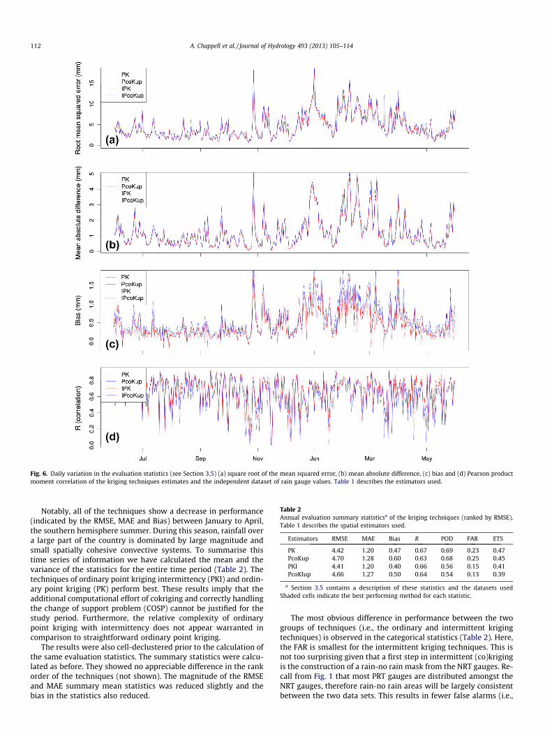
Fig. 6. Daily variation in the evaluation statistics (see Section 3.5) (a) square root of the mean squared error, (b) mean absolute difference, (c) bias and (d) Pearson productmoment correlation of the kriging techniques estimates and the independent dataset of rain gauge values. Table 1 describes the estimators used.

Table 2Annual evaluation summary statisticsa of the kriging techniques (ranked by RMSE).Table 1 describes the spatial estimators used.

Estimators RMSE MAE Bias R POD FAR ETS

PK 4.42 1.20 0.47 0.67 0.69 0.23 0.47PcoKup 4.70 1.28 0.60 0.63 0.68 0.25 0.45PKI 4.41 1.20 0.40 0.66 0.56 0.15 0.41PcoKIup 4.66 1.27 0.50 0.64 0.54 0.13 0.39

a Section 3.5 contains a description of these statistics and the datasets usedShaded cells indicate the best performing method for each statistic.

112 A. Chappell et al. / Journal of Hydrology 493 (2013) 105–114

Notably, all of the techniques show a decrease in performance(indicated by the RMSE, MAE and Bias) between January to April,the southern hemisphere summer. During this season, rainfall overa large part of the country is dominated by large magnitude andsmall spatially cohesive convective systems. To summarise thistime series of information we have calculated the mean and thevariance of the statistics for the entire time period (Table 2). Thetechniques of ordinary point kriging intermittency (PKI) and ordin-ary point kriging (PK) perform best. These results imply that theadditional computational effort of cokriging and correctly handlingthe change of support problem (COSP) cannot be justified for thestudy period. Furthermore, the relative complexity of ordinarypoint kriging with intermittency does not appear warranted incomparison to straightforward ordinary point kriging.

The results were also cell-declustered prior to the calculation ofthe same evaluation statistics. The summary statistics were calcu-lated as before. They showed no appreciable difference in the rankorder of the techniques (not shown). The magnitude of the RMSEand MAE summary mean statistics was reduced slightly and thebias in the statistics also reduced.

The most obvious difference in performance between the twogroups of techniques (i.e., the ordinary and intermittent krigingtechniques) is observed in the categorical statistics (Table 2). Here,the FAR is smallest for the intermittent kriging techniques. This isnot too surprising given that a first step in intermittent (co)krigingis the construction of a rain-no rain mask from the NRT gauges. Re-call from Fig. 1 that most PRT gauges are distributed amongst theNRT gauges, therefore rain-no rain areas will be largely consistentbetween the two data sets. This results in fewer false alarms (i.e.,

A. Chappell et al. / Journal of Hydrology 493 (2013) 105–114 113

estimation of rain when no rain was observed) and represented inthe FAR. The rain-no rain masking of rain areas, however, is likelyto result in proportionally fewer hits (i.e., estimates of rain whenrain was observed) even if the satellite data are indicating rain out-side the prescribed rain area. The result is smaller POD values forthe intermittent kriging compared to the ordinary kriging ap-proaches. Finally, the ETS suggests that overall, the intermittentkriging techniques perform slightly worse than the other tech-niques in terms of their rainfall detection performance, likely dueto the masking of rain-no rain areas based on NRT gauges alone.

5. Discussion

The intermittent technique for the estimation of rainfall (Baran-court et al., 1992) offers an appropriate method of estimating dailyrainfall because it explicitly tackles the occurrence of discretepatches in space and time for daily rainfall fields. Visually, thereare differences between the maps produced with and without thismethod. However, the general patterns are the same in all of themaps indicating that the differences are at the small scale. Thereis also a strong basis for explicitly dealing with the change of sup-port problem (COSP) in the blending of the satellite 3B42RT andrain gauge data. However, the inclusion of the satellite data usingcokriging makes little visual impression on the rainfall map esti-mates. The use of the satellite data does not change the general,large scale, pattern.

For each day’s NRT rain gauge data used to make the estimatesacross Australia, there are approximately twice as many PRT raingauge validation data. The validation data are used in the evalua-tion of the performance of the techniques. Those statistics quantifythe visual differences as being small and consistent over the year(Fig. 6). The results show that all techniques are more similar toeach other than they are to the validation data. Despite consider-able effort to identify the source of bias we were unable to reacha satisfactory conclusion. We know the PRT and NRT samples arebiased in the sense that they represent the wetter parts of the con-tinent than the drier parts of the continent. However, declusteringthe results prior to calculating the statistics made no difference tothe interpretation.

The results indicate that there appears to be no clear benefits ofincluding the satellite data to estimate daily rainfall across Austra-lia, either with or without the intermittent method. Although thesefindings support the results of Krajewski (1987), other studies haveshown improved rainfall estimates by using satellite (e.g., Grimeset al., 1999) and radar (e.g., Velasco-Forero et al., 2009) data. Thisapparent contradiction between our results and the literaturemay be due to the use of a single spatial model for the entire con-tinent for each day. In other words, there may be mixing betweendifferent climate regimes in different parts of Australia. If this ishappening then it is compounded by the accepted practice of glo-bal (continental scale) statistical assessment of performance. How-ever, an investigation of the regional variation and the use of apooled method of estimating the variogram within and betweenregions (e.g., pooled within-class variogram) was beyond the scopeof this study.

The apparent contradiction led us to investigate the effect ofrain gauge number and density on the blending of satellite withrain gauge data (Renzullo et al., 2011). Results showed that withmore than 1000 evenly spaced gauges there is marginal benefitof including the satellite rainfall retrievals in the interpolation ofgauge observations (see online supplementary material). This ap-pears to be because the satellite 3B42RT data improves upongauge-only analyses in (predominantly interior) regions of Austra-lia where gauge densities are less than 4 gauges per 10,000 km2.Bias due to the large density of gauge observations around the

coastal region is likely contained partly within the satellite dataand partly the validation data because of the tendency for gaugesto be correlated with one another in densely sampled areas. Conse-quently, blending the satellite data with gauge data will, relative tothe gauge-based validation, appear as bias. In sparsely sampledareas, the gauge spacing likely exceeds their correlation distance,the satellite data becomes more useful, and the bias is reduced.

There are typically more than 1000 rain gauges available fornear real-time estimation of daily rainfall across Australia. Conse-quently, there is little benefit of using the satellite data to makeestimates at unsampled locations. However, when the change ofsupport problem (COSP) is tackled and the satellite data are com-bined using cokriging, we observe a considerable difference inthe estimation variance. The estimation variance is reduced toapproximately an order of magnitude smaller (Fig. 5) than thepoint kriging of rain gauges alone. Evidently, the use of satellitedata makes a considerable difference to the estimation variance.These results suggest that there are considerable benefits to appro-priately blending the satellite and rain gauge data. However, thosebenefits are not evident in the traditional performance assessmentmethods (Table 2). This is likely caused by those metrics indicatingthe accuracy of the estimation technique and not the amount ofuncertainty in that estimate. In this case, uncertainty is requiredto demonstrate detectable difference in pattern/trend. Unfortu-nately, the issue of uncertainty is beyond the scope of this paperbut is tackled elsewhere using conditional simulation of blendedrainfall estimates (Chappell et al., 2012).

6. Conclusions

Near real-time (NRT) daily rainfall was estimated across Austra-lia using the network of gauges reporting within 24 h of 9 am onthe day of interest. Observations returned outside this timeframewere used to evaluate the performance of the estimates. Account-ing for discrete patches of rainfall in space and time was a valuabletechnique. It performed best on average during the period of thisstudy. However, its additional complexity hardly warranted thesmall improvement in performance over ordinary point kriging.Estimates of daily rainfall made by combining 3B42RT satelliteand rain gauge data were on average, for the study period, worsethan ordinary point kriging. This was probably because the densityof the gauges, particularly in the coastal regions of Australia, wassufficient to provide accurate results without the satellite data.The satellite data will improve upon gauge-only analyses in (pre-dominantly interior) regions of the Australia where gauge densitiesare less than 4 gauges per 10,000 km2. However, the assessment ofthe benefits of including satellite data to the estimates of dailyrainfall is confounded by the use of traditional evaluation statistics.For example, the kriging estimation variance of blended satelliteand gauge data reduced by an order of magnitude compared to kri-ging gauge data alone. The estimation is a rudimentary estimate ofuncertainty since it is largely dependent on the configuration of thesample data. Detection of difference is dependent on several addi-tional sources of error which when combined would provide amore complete assessment of uncertainty. Nevertheless, the re-duced estimation variance indicates an improved ability to detectchange in daily rainfall with potential for trend detection overlonger time periods. The more holistic assessment of (spatial)uncertainty is beyond the scope of this paper but is consideredelsewhere (Chappell and Agnew, 2008; Chappell et al., 2012). Thisstudy shows that the evaluation of performance based on localestimates relative to an independent dataset is only part of theassessment. The estimation variance indicates the role of uncer-tainty in providing a more realistic assessment of a technique’sperformance within the context of detecting change.

114 A. Chappell et al. / Journal of Hydrology 493 (2013) 105–114

Acknowledgements

This work was supported under the Water Information Re-search and Development Alliance (WIRADA) between the Bureauof Meteorology and CSIRO Water for a Healthy Country flagship.We are grateful for the support of Dr. Andrew Frost in arranging ac-cess to the daily gauge data from the Bureau of Meteorology. Weare grateful to the anonymous reviewers whose comments didmuch to improve the manuscript. Any omissions or errors in themanuscript remain the responsibility of the authors.

Appendix A. Supplementary material

Supplementary data associated with this article can be found, inthe online version, at http://dx.doi.org/10.1016/j.jhydrol.2013.04.024.

References

Atkinson, P.M., Webster, R., Curran, P.J., 1994. Cokriging with airborne MSS imagery.Remote Sens. Environ. 50, 335–345.

Barancourt, C., Creutin, J.D., Rivoirard, J., 1992. A method for delineating andestimating rainfall fields. Water Resour. Res. 28 (4), 1133–1144.

Chappell, A., 1998. Using remote sensing and geostatistics to map 137Cs-derived netsoil flux in south-west Niger. J. Arid Environ. 39, 441–455, http://dx.doi.org/10.1006/jare.1997.0365.

Chappell, A., Agnew, C.T., 2008. How certain is desiccation in west African Sahelrainfall (1930–1990)? J. Geophys. Res. 113, D07111, http://dx.doi.org/10.1029/2007JD009233.

Chappell, A., Haylock, M., Renzullo, L., 2012. Spatial uncertainty to determinereliable daily precipitation maps.. J. Geophys. Res. 117, D17115, http://dx.doi.org/10.1029/2012JD017718.

Clarke, R.T., Buarque, D.C., De Paiva, R.C.D., Collischonn, W., 2011. Issues of spatialcorrelation arising from the use of TRMM rainfall estimates in the BrazilianAmazon. Water Resour. Res. 47 (5), W05539.

Creutin, J.C., Obled, C., 1982. Objective analysis and mapping techniques for rainfallfields: an objective comparison. Water Resour. Res. 18 (2), 413–431.

Deutsch, C.V., 1989. DECLUS: a fortran 77 program for determining optimum spatialdeclustering weights. Comput. Geosci. 15 (3), 325–332.

Deutsch, C.V., Journel, A.G., 1998. GSLIB: Geostatistical Software Library and User’sGuide. Oxford University Press, Oxford, pp. 369.

Ebert, E.E., Janowiak, J.E., Kidd, C., 2007. Comparison of near-real-time precipitationestimates from satellite observations and numerical models. Bull. Am.Meteorol. Soc. 88, 47–64. http://dx.doi.org/10.1175/BAMS-88-1-47.

Goovaerts, P., 2000. Geostatistical approaches for incorporating elevation into thespatial interpolation of rainfall. J. Hydrol. 228, 113–129.

Gotway, C.A., Young, L.J., 2002. Combining incompatible spatial data. J. Am. Stat.Assoc. 97 (458), 632–648.

Grimes, D.I.F., Pardo-Igúzquiza, E., 2010. Geostatistical analysis of rainfall.Geograph. Anal. 42, 136–160.

Grimes, D.I.F., Pardo-Igúzquiza, E., Bonifacio, R., 1999. Optimal areal rainfallestimation using raingauges and satellite date. J. Hydrol. 222, 93–108.

Hofstra, N., Haylock, M., New, M., Jones, P., Frei, C., 2008. The comparison of sixmethods for the interpolation of daily European climate data. J. Geophys. Res.113, D21110. http://dx.doi.org/10.1029/2008JD010100.

Huffman, G.F., Adler, R.F., Arkin, P., Chang, A., Ferraro, R., Gruber, A., Janowiak, J.,McNab, A., Rudolf, B., Schneider, U., 1997. The global precipitation climatologyproject (GPCP) combined precipitation dataset. Bull. Am. Meteorol. Soc. 78 (1),5–20.

Huffman, G.F., Adler, R.F., Bolvin, D.T., Gu, G., Nelkin, E.J., Bowman, K.P., Hong, Y.,Stocker, E.F., Wolff, D.B., 2007. The TRMM multisatellite precipitation analysis(TMPA): quasi-global, multiyear, combined-sensor precipitation estimates atfine scales. J. Hydrometeorol. 8, 38–55.

IPWG, 2011. International Precipitation Working Group, <http://www.isac.cnr.it/’ipwg/validation.html>.

Isaaks, E.H., Srivastava, R.M., 1989. An Introduction to Applied Geostatistics. OUP,New York.

Jeffrey, S.J., Carter, J.O., Moodie, K.B., Beswick, A.R., 2001. Using spatial interpolationto construct a comprehensive archive of Australian climate data. Environ.Model. Software 66, 309–330.

Jones, D.A., Wang, W., Fawcett, R., 2009. High-quality spatial climate data-sets forAustralia. Aust. Meteorol. Oceanogr. J. 58 (4), 233–248.

Journel, A.G., Huijbregts, C.J., 1978. Mining Geostatistics. Academic Press, London.Joyce, R.J., Janowiak, J.E., Arkin, P.A., Xie, P., 2004. CMORPH: a method that produces

global precipitation estimates from passive microwave and infrared data athigh spatial and temporal resolution. J. Hydrometeorol. 5, 487–503.

Krajewski, W.F., 1987. Cokriging radar-rainfall and rain gauge data. J. Geophys. Res.92, 9571–9580.

Kubota, T., Shige, S., Hashizume, H., Aonashi, K., Takahashi, N., Seto, S., et al., 2007.Global precipitation map using satelliteborne microwave radiometers by theGSMaP Project: production and validation. IEEE Trans. Geosci. Remote Sens. 45(7), 2259–2275.

Kummerow, C., Simpson, J., Thiele, O., Barnes, W., Chang, A.T.C., Stocker, E., Adler,R.A., Hou, A., Kakar, R., Wentz, F., Ashcroft, P., Kozu, T., Hong, Y., Okamoto, K.,Iguchi, T., Kuroiwa, H., Im, E., Haddad, Z., Huffman, G., Ferrier, B., Olson, W.S.,Zipser, E., Smith, E.A., Wilheit, T.T., North, G., Krishnamurti, T., Nakamura, K.,2000. The status of the tropical rainfall measuring mission (TRMM) after twoyears in orbit. J. Appl. Meteorol. 39, 1965–1982.

Kyriakidis, P., 2004. A geostatistical framework for area to point interpolation.Geograph. Anl. 36 (3), 259–289.

Laslett, G.M., 1994. Kriging and splines: an empirical comparison of their predictiveperformance in some applications. J. Am. Stat. Assoc. 89, 391–409.

Laslett, G.M., McBratney, A.B., 1990. Estimation and implications of instrumentaldrift, random measurement error and nugget variance of soil attributes – a casestudy for soil pH. J. Soil Sci. 41, 451–471.

Laslett, G.M., McBratney, A.B., Pahl, P.J., Hutchinson, M.F., 1987. Comparison ofseveral spatial prediction methods for soil pH. J. Soil Sci. 38, 325–341.

Lebel, T., Bastin, G., Obled, C., Creutin, J.D., 1987. On the accuracy of areal rainfallestimation: a case study. Water Resour. Res. 23, 2123–2134.

Li, M., Shao, Q., 2010. An improved statistical approach to merge satellite rainfallestimates and raingauge data. J. Hydrol. 385, 51–64. http://dx.doi.org/10.1016/j.jhydrol.2010.01.023.

Renzullo, L.J., Chappell, A., Raupach, T., Dyce, P., Ming, L., Shao, Q., 2011. Anassessment of statistically blended satellite-gauge precipitation data for dailyrainfall analysis in Australia. In: International Remote Sensing of EnvironmentConference Proceedings, Sydney, Australia.

Tian, Y., Peters-Lidard, C.D., 2011. A global map of uncertainty in satellite-basedprecipitation measurements. Geophys. Res. Lett. 37, 6. http://dx.doi.org/10.1029/2010GL046008, L2440.

Velasco-Forero, C., Sempere-Torres, D., Cassiraga, E.F., Gomez-Hernandez, J.J., 2009.A non-parametric automatic blending methodology to estimate rainfall fieldsfrom rain gauge and radar data. Adv. Water Resour. 32, 986–1002.

Vila, D.A., de Goncalves, L.G.G., Toll, D.L., Rozante, J.R., 2009. Statistical evaluation ofcombined daily gauge observations and rainfall satellite estimates overcontinental South America. J. Hydrometeorol. 10, 533–543.

Webster, R., Oliver, M.A., 2001. Geostatistics for Environmental Scientists. Wiley,Chichester, UK.