Evaluating AVI and DRASTIC for Assessing Pollution ... · Aquifer Vulnerability and Nitrate...

I 92+ .# 7 8

I I I I I I

Evaluating AVI and DRASTIC for Assessing Pollution Potential in the Lower Fraser Valley, British Columbia:

Aquifer Vulnerability and Nitrate Occurrence

I I I I I

I I I I

i

1

M. Wei, P. Eng. Aquifer Assessment and Monitoring Unit

Groundwater Section

July, 1998

Ministry of Envi ronrnent, Lands and Parks

Water Management Branch

Canadian Cataloguing in Publication Data Wei, M.

Evaluating AVI and DRASTIC f o r assessing pollution potential in the lower Fraser Valley, British Columbia

Includes bibliographical references: p. ISBN 0-7726-3641-9

1. Groundwater - Pollution - British Columbia - Lower Mainland - Measurement. 2. Water - Pollution potential - British Columbia - Lower Mainland - Measurement. 3 . Aquifers - British Columbia - Lower Mainland. 4. Nitrates - Environmental aspects - British Columbia - Lower Mainland. I. British Columbia. Ministry of Environment, Lands and Parks. 11. Title.

I I I I I I I

I I I

i

TD426.W44 1998 363.739'42'0971137 C98-960224-9

I I

I I I I I I I I I I I I I I I I

i

AVI and DRASTIC: Evaluating Aquifer Vulnerability and Nitrate Occurrence

Evaluating AVI and DRASTIC for Assessing Pollution Potential in the Lower Fraser Valley, British Columbia: Aquifer Vulnerability and Nitrate Occurrence

by M. Wei, Groundwater Section, Water Management Branch, Ministry of Environment, Lands and Parks

Executive Summary AVI and DRASTIC indexes calculated for 169 wells in the Lower Fraser Valley, British Columbia (BC) show generally consistent results. Low AVI and high DRASTIC indexes correspond with high vulnerability while high AVI and low DRASTIC indexes correspond with low vulnerability. AVI and DRASTIC indexes show a bimodal distribution with data points clustered around either high vulnerability or low vulnerability with very few in the moderate vulnerability range. High vulnerability is associated with unconfined conditions and low vulnerability is generally associated with confined conditions. The bimodal distribution likely reflects the confined and unconfined nature of aquifers in the Lower Fraser Valley. The AVI and DRASTIC indexes are also consistent with the vulnerability of the aquifers as designated under the BC Aquifer Classification System.

AVI and DRASTIC appear to correlate with occurrence of water quality degradation by nitrate in the Lower Fraser Valley. Most of the elevated nitrates (NO3-N > 3 mgL) occur in wells where AVI values are <-1 and DRASTIC indexes are >160. Elevated nitrates are not expected in areas where the DRASTIC index is ~ 1 0 0 . Nitrate exceeding the drinking water guideline (N03-N > 10 m a ) could occur in the Lower Fraser Valley (depending on land use activities) where AVI values are <-I and DRASTIC indexes are greater than 120, based on water quality data in the study area.

Presence of fine-grained lenses at a particular well can cause anomalously high AVI results to be calculated. Interpretation of pollution potential in a local area should, therefore, not be made based on the AVI index calculated for a single well but should also include AVI indexes from other wells nearby. A key to properly assessing pollution potential is to have good quality well records.

Both AVI and DRASTIC appear suitable for predicting pollution potential for unconsolidated aquifers in southwestern BC. The choice of which method to use for aquifer vulnerability mapping may depend, in the end, on additional factors such as ease of use (AVI is less subjective than DRASTIC) and on the information available (e.g., soils mapping, recharge estimates, etc.). The suitability of AVI and DRASTIC for predicting pollution potential in fractured bedrock aquifers in BC needs to be further evaluated.

711 3/98 1

I AVI and DRASTIC: Evaluating Aquifer Vulnerability and Nitrate Occurrence

Table of Contents

Executive Summary 1 Introduction 1.1 AVI 1.2 DRASTIC 1.3 Assumptions 1.4 Study Objectives 1.5 Study Area 2 Methods 3 Results and Discussions 3.1 Comparing AVI and DRASTIC Indexes 3.2 Comparing AVI and DRASTIC Indexes to Aquifer Classification 3.3 Comparing AVI and DRASTIC Indexes to Water Quality 3.4 Uses of AVI and DRASTIC Indexes for Community Well Protection 4 Conclusions and Recommendations 5 References 6 Acknowledgments

List of Figures Figure 1. Study area showing the study wells, the seventeen unconfined aquifers and two

Figure 2. Histogram of AVI values for the study wells. Figure 3. Histogram of DRASTIC indexes for the study wells. Figure 4. Correlation analysis of the DRASTIC factors for the study wells. Figure 5. Scatter plot of AVI versus DRASTIC values for the study wells. Figure 6. Box plot of AVI values for each aquifer vulnerability classification designation. Figure 7. Box plot of DRASTIC indexes for each aquifer vulnerability classification

Figure 8. Percentage of study wells with NO3-N > 3 mg/L per AVI category (number of

Figure 9. Percentage of study wells with N03-N > 3 mg/L per DRASTIC category (number

Figure 10. Plot of NO3-N versus AVI values. Figure 1 1. Plot of N03-N versus DRASTIC indexes.

bedrock aquifers (the twelve confined aquifers are not shown).

designation.

wells in brackets).

of wells in brackets).

List of Tables Table 1. AVI categories. Table 2. Hydraulic conductivity ‘K’ estimates for various sediments. Table 3. Summary of recharge for aquifers in the study area and ratings for the DRASTIC

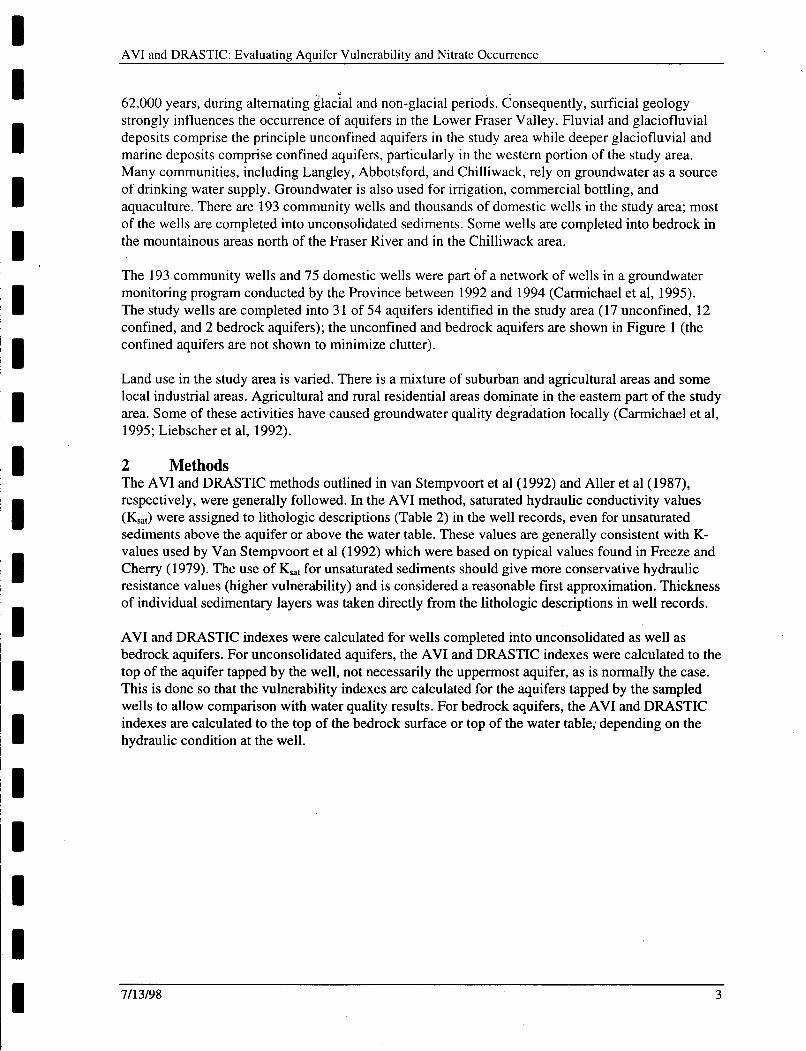
Table 4. Aquifer media descriptions and ratings for the DRASTIC method. Table 5. Soil descriptions and ratings for the DRASTIC method. Table 6. Impact of vadose zone categories and ratings for the DRASTIC method. Table 7. Aquifer hydraulic conductivity categories and ratings for the DRASTIC method.

method.

List of Appendexes Appendix A. Summary of Aquifer Vulnerability Mapping Methods in Select Jurisdictions. Appendix B. AVI and DRASTIC Values for the Study Wells

1

1 1 2 2 2 2 3 7 9

11 12 16 17 18 20

at back

8 8 9

11 12 12

14

14

15 16

2 4 5

6 6 7 7

21 24

i I I I E I I I I I

I I I I I I

i

11 711 3/98


I I I I I I I I I I I I I I I I I I

1 Introduction British Columbia (BC) has an abundance of good quality groundwater (BC Environment, 1994). A significant portion of the Province's groundwater supply comes from shallow, unconfined aquifers that receive recharge directly from infiltration of precipitation or from surface water bodies such as rivers and lakes. These unconfined aquifers are prone to impacts from human activities which have resulted in incidences of water quality degradation (BC Environment, 1997; BC Environment, 1996; Carmichael et al, 1995; Wei et al, 1993; Liebscher et al, 1992). A cost-effective way to protect water quality is to map and assess the vulnerability' of aquifers to assist in planning land use activities and, thereby, minimizing water quality impacts (Sacre and Patrick, 1994; Piteau Associates and Turner Groundwater Consultants, 1993).

There is a surprising number of methods for characterizing aquifer vulnerability (see Vrba and Zaporozec, 1994). Many of the methods were developed empirically, based on the local hydrogeologic settings, data sets, and intended objectives of the mapping project. Some of these methods are summarized in Appendix A. However, few comparisons of these methods have been done. Two methods currently being used by other Provinces and States and which are being considered for use in BC are: AVI (Aquifer Vulnerability Index), developed by the Prairie Provinces Water Board (Van Stempvoort et al, 1992), and DRASTIC, developed by US EPA (Aller et al, 1987). Rosen (1 994) did a conceptual evaluation of DRASTIC and concluded that DRASTIC had some advantages and is relevant for assessing groundwater pollution potential in southwest Sweden. Ronneseth et a1 (1995) did a mapping evaluation of both AVI and DRASTIC in the Abbotsford- Aldergrove area, east of Vancouver, BC and concluded that both methods appear suitable for use in shallow, unconsolidated, glaciated terrains in southwestern BC.

However, few studies have been done to evaluate how aquifer vulnerability determined from of AVI and DRASTIC correlate with actual water quality impacts from human activities; the suitability of these methods for predicting the pollution potential of aquifers has not been thoroughly validated. Kalinski et a1 (1994) found that DRASTIC indexes correlated with frequency of volatile organic compound (VOC) detections in municipal wells in Nebraska. Garrett et a1 (1989) concluded, on the other hand, that DRASTIC was a poor indicator of hydrocarbon and road salt contamination in Maine, probably because DRASTIC does not deal very well with fate and transport of contaminants in Maine's fractured bedrock aquifers. Ronneseth et a1 (1995) compared AVI and DRASTIC against nitrate-nitrogen concentrations for a limited number of wells in the Abbotsford-Aldergrove area. This report evaluates how well AVI and DRASTIC correlate with actual water quality (specifically nitrate) impacts from human activities in the Lower Fraser Valley.

1.1 AVI AVI quantifies an aquifer's vulnerability at any given location by the hydraulic resistance (c) to the vertical flow of water through the geologic sediments above the aquifer. The hydraulic resistance is calculated from two variables: the thickness (d) of each sedimentary layer above the uppermost aquifer and the hydraulic conductivity (K) of each of the layers (Equation 1).

Hydraulic resistance, c = Cdi / Kj , for layers 1 to i (1)

Aquifer vulnerability is defined here as the intrinsic vulnerability of an aquifer to contamination strictly as a function of the physical characteristics of the aquifer and the overlying soil and geological sediments (see Vrba and Zaporozec, 1994). The type and intensity of human activities above an aquifer are not criteria in determining aquifer vulnerability but rather in the overall assessment of an aquifer's actual risk to contamination.

7/13/98 1

AVI and DRASTIC: Evaluating Aauifer Vulnerabilitv and Nitrate Occurrence

Hydraulic resistance (c) has the dimension of time (e.g. years) and represents the flux-time per unit head gradient for water travelling downward through the various sediment layers to the aquifer. The lower the hydraulic resistance (c), the greater the vulnerability. A vulnerability map can be constructed by calculating the logarithm of the hydraulic resistance (log c) for each well and delineating areas of similar log c (AVI) values. The resultant areas represent areas of different resistance which are grouped into the vulnerability categories in Table 1. AVI defines an aquifer as any water-bearing zone of > 0.6 m thickness with at least one well tapping it.

1.2 DRASTIC DRASTIC is a composite rating of the Depth to water, net Recharge, Aquifer media, Soil media, Topography, Impact of the vadose zone and the hydraulic Conductivity of the aquifer (Equation 2).

DRASTIC Index = 5D + 4R + 3A + 2s + 1T + 51 + 3C (2)

In equation (2), the numbers represent the relative weights and the letters correspond to each of the seven physical parameters. DRASTIC incorporates a relative ranking scheme that uses a combination of weights and ratings to produce a numerical value called the DRASTIC index. Hydrogeologic settings combine with DRASTIC indexes to form polygon areas on a map. Each polygon area represents similar hydrogeological conditions and consequently similar vulnerability. The DRASTIC index ranges from 23 to 230; the higher the DRASTIC index, the greater the vulnerability. Although DRASTIC is physically based, the final DRASTIC index, unlike AVI, has no physical units, but rather is a numerical index.

1.3 Assumptions Both AVI and DRASTIC assume that the potential contaminant source is at or near the land surface, the contaminant has the same behaviour as water, recharge to the aquifer is from vertical infiltration of precipitation, and flow in the vadose (and saturated) zone above the aquifer is vertically downward. For a more detailed description of AVI and DRASTIC, refer to van Stempvoort et a1 (1992) and Aller et a1 (1987), respectively.

1.4 Study Objectives The objectives of this study are to: 0 determine AVI and DRASTIC indexes for all community wells and select private wells in the

Lower Fraser Valley (Figure 1) to quantify the aquifer’s vulnerability to contamination at those specific well locations and evaluate how water quality impacts from human activities relate to the aquifer vulnerability indexes calculated.

1.5 Study Area The study area is situated in the Lower Fraser Valley, east of Vancouver (Figure 1). Unconsolidated deposits, up to 300 m thick, underlie the area; most of the sediments were deposited within the last

2 7/13/98

I I I I I I I I I I I I I I I I I I I

I I

II I I I I I I I I I I I I I I I

~I

AVI and DRASTIC: Evaluating Acluifer Vulnerabilitv and Nitrate Occurrence

62,000 years, during alternating glacial and non-glacial periods. Consequently, surficial geology strongly influences the occurrence of aquifers in the Lower Fraser Valley. Fluvial and glaciofluvial deposits comprise the principle unconfined aquifers in the study area while deeper glaciofluvial and marine deposits comprise confined aquifers, particularly in the western portion of the study area. Many communities, including Langley, Abbotsford, and Chilliwack, rely on groundwater as a source of drinking water supply. Groundwater is also used for imgation, commercial bottling, and aquaculture. There are 193 community wells and thousands of domestic wells in the study area; most of the wells are completed into unconsolidated sediments. Some wells are completed into bedrock in the mountainous areas north of the Fraser River and in the Chilliwack area.

The 193 community wells and 75 domestic wells were part of a network of wells in a groundwater monitoring program conducted by the Province between 1992 and 1994 (Carmichael et al, 1995). The study wells are completed into 31 of 54 aquifers identified in the study area (17 unconfined, 12 confined, and 2 bedrock aquifers); the unconfined and bedrock aquifers are shown in Figure 1 (the confined aquifers are not shown to minimize clutter).

Land use in the study area is varied. There is a mixture of suburban and agricultural areas and some local industrial areas. Agricultural and rural residential areas dominate in the eastern part of the study area. Some of these activities have caused groundwater quality degradation locally (Carmichael et al, 1995; Liebscher et al, 1992).

2 Methods The AVI and DRASTIC methods outlined in van Stempvoort et a1 (1992) and Aller et a1 (1987), respectively, were generally followed. In the AVI method, saturated hydraulic conductivity values (KSat) were assigned to lithologic descriptions (Table 2) in the well records, even for unsaturated sediments above the aquifer or above the water table. These values are generally consistent with K- values used by Van Stempvoort et al(1992) which were based on typical values found in Freeze and Cherry (1979). The use of K,,, for unsaturated sediments should give more conservative hydraulic resistance values (higher vulnerability) and is considered a reasonable first approximation. Thickness of individual sedimentary layers was taken directly from the lithologic descriptions in well records.

AVI and DRASTIC indexes were calculated for wells completed into unconsolidated as well as bedrock aquifers. For unconsolidated aquifers, the AVI and DRASTIC indexes were calculated to the top of the aquifer tapped by the well, not necessarily the uppermost aquifer, as is normally the case. This is done so that the vulnerability indexes are calculated for the aquifers tapped by the sampled wells to allow comparison with water quality results. For bedrock aquifers, the AVI and DRASTIC indexes are calculated to the top of the bedrock surface or top of the water table; depending on the hydraulic condition at the well.

7/13/98 3


Hydraulic Conductivity * (K) Estimates for Various Sediments

Sediment Type ** (K) metredday (approx.)

gravel sand and gravel, gravelly sand, sandy

gravel, coarse sand gravel, sand, and silt, medium sand, ’

sand fine sand, silty sand and gravel, very

fine sand, silty sand gravelly silt, sandy silt, silt, clayey

gravel, clayey sand clayey silt, gravel till, sandy till,

fractured bedrock

clay, gravelly clay, sandy clay, silty clay

clayey till, till, hardpan

1000 100

10

1

0.1

0.001

0.00001 0.00000 1

* (K) Saturated ** In reality, each of these sediment types has a range of values over several orders of magnitude; the values here are representative values.

Table 2. Hydraulic conductivity ‘K’ estimates for various sediments. I

With DRASTIC, individual ratings and total DRASTIC indexes were determined for each well location. The depth to water table (or top of aquifer) was determined directly from well records. Average net recharge was estimated for specific aquifers using recharge information in Table 9.2 of the Groundwater Resources of British Columbia (BC Environment, 1994). Recharge estimates for other aquifers were inferred from aquifers comprising similar deposits and in similar physical settings. Table 3 shows the estimated recharge values for all the aquifers tapped by the study wells. Aquifer recharge is assumed to be uniform for the whole aquifer. For wells not completed in any identified aquifers in Table 3, a rating for recharge of 9 was given for unconfined water-bearing zones and 6 for confined water-bearing zones for wells < 30m and 3 for confined water-bearing zones in wells > 30 m deep.

4 711 3/98

I I I I I I I I I I I I I I I I

I I I I I I I II ~I ~I I I I

Lake Erroch/Derroche Creek Nicomen Slough

Norrish Creek Hatzic Prairie Abbotsford-Sumas

I

>10 9

>10 9 WAiea should be similar to Chawuthen, Chehalis and Chilliwack- Rosedale

>10 9 from BC Environment (1993) >10 9 WArea should be similar to Norrish Creek 22 9 from BC Environment (1993)

AVI and DRASTIC: Evaluating Aauifer Vulnerability and Nitrate Occurrence

Mission Floodplain

Mission Grant Hill Columbia Valley

Miracle Vallev Glen Valley

Table 3. Summary of recharge for aquifers in the study area and ratings for the DRASTIC method.

~ ~ _ _ _ _

>10 9 WArea should be similar to Chawuthen, Chehalis and Chilliwack- Rosedale

8? 8?

>10 9 WArea should be similar to Abbotsford-Sumas -10 -9

3 3 R/Area should be similar to White Rock (verv low)

Vedder River Fan I 24 I 9 lfrom BC Environment (1993)

Aldergrove

IChilliwack River I 26 I 9 IfromBCEnvironment (1993)

11 I 6 lfrom BC Environment (1993) but averaged for a larger aquifer area

West of Aldergrove Hopington Fort Langley East Pitt River

Langley/Brookswood

South of Murrayville South of Hopington

IMt. Lehman I > l o I 6 I

3? 3? 8 8 from BC Environment (1993) 12 9 from BC Environment (1993)

WArea should be similar to Chawuthen, Chehalis and Chilliwack- Rosedale

22 9 from BC Environment (1993) 3? 3? 3 3

>10 9

WArea should be similar to White Rock (very low)

Grandview Nicomekl-Serpentine

Clayton Upland (Lower) McMillan Island

Clayton Upland (Upper)

3 3 3 3 3? 3? 3 3

>10 9

R/Area should be similar to White Rock (very low) R/Area should be similar to White Rock (very low)

R/Area should be similar to White Rock (very low) WArea should be similar to Chawuthen, Chehalis and Chilliwack- Rosedale

IBeaver River I 3 I 3 IWArea should be similar to White Rock (very low)

ILangley UplandInter-till I 3? I 3? I

Ratings for aquifer media and aquifer K-values were assigned based on lithologic descriptions from well records (Table 4). Where lithology is layered, an arithmetic average K-value was estimated. Ratings for soil media and topographic slope for each well location were determined from 1:25,000 scale soil mapping (Luttmerding, 1981) and 1:SOOO and 1:2000 scale topographic (2 metre contours) mapping, respectively. In the 092H area, where soils mapping were not available, Armstrong’s (1980) suficial geology map was used to infer the soils in that area (Table 5). For impact of the

711 3/98 5


vadose zone, the equivalent saturated vertical K-value for each well was calculated (total depth to water table or top of aquifer divided by the sum of the hydraulic resistance of the individual sedimentary layers) instead of relying strictly on the lithologic description of sediments above the aquifer or above the water table. Ratings for impact of the vadose zone were then determined by relating the equivalent vertical K-value of the vadose zone to the equivalent lithologic descriptions in Table 6. Ratings for aquifer K-values were assigned using Table 7. Where the lithology is layered, the arithmetic average K-value was estimated.

ings for the DRASTIC method.

Table 5. Soil descriptions and ratings for the DRASTIC method. Soil name (and surlicial geologic deposit) Perviousness S

“ I * Rating

Coghlan, Hamson, Lehman, Sardis, (slope wash deposits, stream deposits, Abbotsford Outwash, Huntingdon Gravel and other Pre-Sumas Till fluvial deoosits. exDosed bedrock)

10

Columbia, Chehalis, Roach, (Fraser floodplain I rapidly pervious 9 sand deposits, lacustrine sand deposits) Buntzen, Bose, Cannel, Capilano, Defehr, Elk, Errock, Eunice, Grevell, Glen Valley, Heron, Isar, Judson, Lumbum, Lynden, Stave, Sunshine Keystone, Laxton Monroe, Matsqui

Abbotsford, Durieu, Hopedale, Lonzo Creek, McElvee, Marble Hill, Neaves, Peardonville, Page, Steelhead Bates, Fairfield, Nicholson, Milner, Ryder, (Fraser floodplain silt and clay deposits, lacustrine silt and clay deposits) Albion, Banford, Beharrel, Berry, Calkins, Carvolth, Ross, Scat, Whatcom, (Sumas Till)

rapidly pervious

rapidly pervious, rapidly to moderately pervious (Elk, Sunshine), moderately pervious (Glen Valley, Judson, Lumbum)

rapidly to moderately pervious and moderately pervious (Monroe) moderately pervious, rapidly to moderately pervious (Hopedale), moderately pervious but slow in subsoil (Steelhead) moderately pervious, moderately to slowly pervious (Milner)

8

rapidly pervious I 6

5

4

moderately to slowly pervious, moderately pervious (Banford, Calkins), slowly pervious (Carvolth, Scat)

3

I I

6 7/13/98

I I



I no vadose zone I

Table 7. Aquifer hydraulic conductivity categories and ratings for the DRASTIC method.

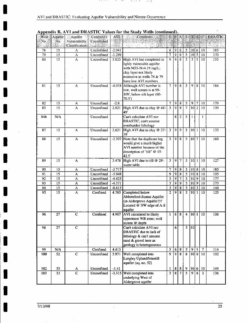
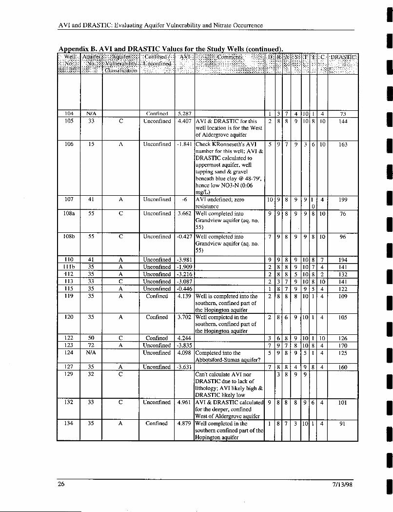
3 Results and' Discussions AVI and DRASTIC indexes were calculated for 169 of the 253 study wells (103 community wells and 66 private wells). Vulnerability indexes could not be calculated for the other 84 wells (77 community wells and 7 private wells) due to lack of lithology in the well records. Vulnerability indexes for the 169 study wells are tabulated in Appendix B.

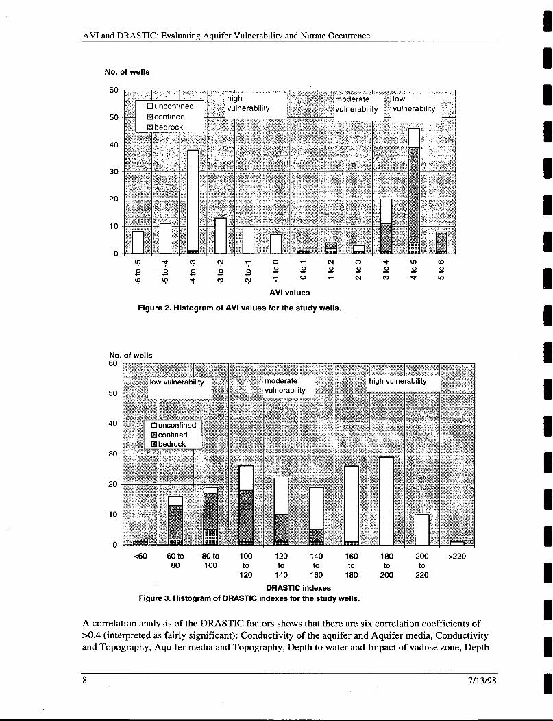
AVI values range from a low of -62 (extremely high vulnerability) to a high of 5.56 (extremely low vulnerability). DRASTIC indexes range from a high of 220 (highly vulnerable) to a low of 50 (low vulnerability). Histograms of AVI and DRASTIC indexes (Figures 2 and 3) show a bimodal distribution. Both AVI and DRASTIC indexes group into very high and high vulnerability (AVI values of e0 and DRASTIC indexes of >160) and low vulnerability (AVI values greater than 3 and DRASTIC indexes of ~ 1 2 0 ) categories with very few indexes in the moderate vulnerability range. The bimodal nature of the DRASTIC histogram is less pronounced, because the combination of seven DRASTIC factors help dampen this. Rosen (1 994) concluded that the fairly large number of parameters in DRASTIC tends to limit variability of the results. Both histograms show that high vulnerability is associated with unconfined conditions while low vulnerability is associated with mostly confined conditions3. The few wells associated with unconfined conditions having high AVI and low DRASTIC indexes are wells that encountered clay or till lenses e3 m thick. The presence of localized clay or till lenses significantly impacts on the vulnerability index calculation, causing the vulnerability to be under-estimated. AVI and DRASTIC indexes for most of the 11 bedrock wells in the study reflect mostly low to moderate vulnerability.

AVI values of -6 were assigned where the hydraulic resistance, c, was zero (e.g., where depth to water was zero). Wells that have >3 m of likely low permeability sediments (e.g. clay, till) are designated as confined (even though they may be completed

into an essentially unconfined aquifer). Wells that have e3 m of likely low permeability sediments are designated as unconfmed; the likely low permeability sediments are interpreted as lenses and are assumed to be not areally extensive.

7/13/98 7


No. of wells

60

50

40

30

20

10

0 7 0 7 cu 0 d In ul

0 0 F 0 7 cu m d In

r 7 3 9 c 0 - 0 - 0 - 0 - ? r P 3 9

c 0 - o c 0 - 0 - 0 - O c

AVI values

Figure 2. Histogram of AVI values for the study wells.

No. of wells

e60 60to 80to 100 120 140 160 180 200 >220 80 100 to to to to to to

DRASTIC indexes

120 140 160 180 200 220

Figure 3. Histogram of DRASTIC indexes for the study wells.

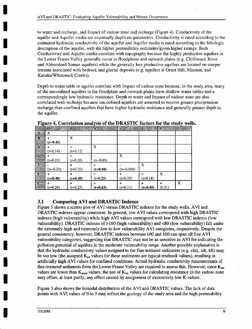
A correlation analysis of the DRASTIC factors shows that there are six correlation coefficients of >0.4 (interpreted as fairly significant): Conductivity of the aquifer and Aquifer media, Conductivity and Topography, Aquifer media and Topography, Depth to water and Impact of vadose zone, Depth

8 7/13/98

D D I I I D I I I I I I D I I I I I I



to water and recharge, and Impact of vadose zone and recharge (Figure 4). Conductivity of the aquifer and Aquifer media are essentially duplicate parameters. Conductivity is rated according to the estimated hydraulic conductivity of the aquifer and Aquifer media is rated according to the lithologic description of the aquifer, with the higher permeability sedimentsylgiven higher ratings. Both Conductivity and Aquifer media correlate with topography because the highly productive aquifers in the Lower Fraser Valley generally occur in floodplains and outwash plains (e.g. Chilliwack River and Abbotsford-Sumas aquifers) while the generally less productive aquifers are located on steeper terrains associated with bedrock and glacial deposits (e.g. aquifers at Grant Hill, Mission, and Kanakflhonnock Creeks).

Depth to water table or aquifer correlate with Impact of vadose zone because, in the study area, many of the unconfined aquifers in the floodplain and outwash plains have shallow water tables and a correspondingly low hydraulic resistance. Depth to water and Impact of vadose zone are also correlated with recharge because unconfined aquifers are assumed to receive greater precipitation recharge than confined aquifers that have higher hydraulic resistance and generally greater depth to the aquifer.

S.

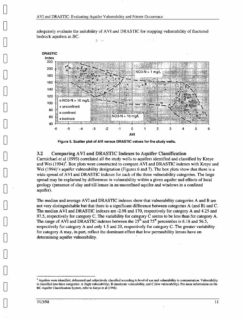
3.1 Figure 5 shows a scatter plot of AVI versus DRASTIC indexes for the study wells. AVI and DRASTIC indexes appear consistent. In general, low AVI values correspond with high DRASTIC indexes (high vulnerability) while high AVI values correspond with low DRASTIC indexes (low vulnerability). DRASTIC indexes of >160 (high vulnerability) and e80 (low vulnerability) fall under the extremely high and extremely low to low vulnerability AVI categories, respectively. Despite the general consistency, however, DRASTIC indexes between 100 and 160 can span all five AVI vulnerability categories, suggesting that DRASTIC may not be as sensitive as AVI for indicating the pollution potential of aquifers in the moderate vulnerability range. Another possible explanation is that the hydraulic conductivity values assigned to the fine-textured sediments (e.g. clay, silt, till) may be too low (the assigned K,,, values for these sediments are typical textbook values), resulting in artificially high AVI values for confined conditions. Actual hydraulic conductivity measurements of fine-textured sediments from the Lower Fraser Valley are required to assess this. However, since K,,, values are lower than K,,, values, the use of K,,, values for calculating resistance in the vadose zone may offset, at least partly, any effect caused by assignment of excessively low K-values.

Comparing AVI and DRASTIC Indexes

Figure 5 also shows the bimodal distribution of the AVI and DRASTIC values. The lack of data points with AVI values of 0 to 3 may reflect the geology of the study area and the high permeability

7/13/98 9


contrast of coarse and fine textured sediments in calculating the hydraulic resistance. The dashed lines in Figure 5 bound the region where AVI and DRASTIC values for the study area are likely to plot. AVI and DRASTIC values plotting outside of this region are likely not physically plausible and may be anomalous.

There are several wells drilled through unconfined materials that have anomalously high AVI and/or low DRASTIC indexes (low vulnerability). High AVI and/or low DRASTIC indexes for wells drilled through essentially unconfined sediments can largely be explained by the occurrence of till or clay lenses. For example, the high AVI value for well 80 is a due to the presence of a thin clay layer from 0 m to 2.4 m depth. This clay layer is likely not extensive because it is not encountered in wells 78 nor 79 nearby. The presence of a thin clay or till layer significantly raises the hydraulic resistance because of the low K-value assigned to these sediments. For example, a 0.3 m thick clay layer with a K-value of d d a y has a hydraulic resistance of 835 years (log c = 2.92). The presence of 0.3 m lens of clay in an otherwise clean sand and gravel aquifer would cause the AVI value at the well to increase from a negative value to 2.9, giving a false impression of low vulnerability. AVI values calculated from individual wells should, therefore, be interpreted with caution; AVI values from neighbouring wells should be considered in assessing the vulnerability in a local area. No wells drilled through confining sediments have AVI values of e1 or DRASTIC indexes of ~ 1 6 0 . This illustrates the effect of low-K lenses in increasing hydraulic resistance.

Two wells (48 and 49) are completed into sandstone bedrock of the Grant Hill aquifer. Their high AVI and low DRASTIC values are due to the low K-value assigned to the bedrock. In fractured bedrock aquifers in many parts of BC where the hydraulic conductivity of the bulk bedrock is relatively low, both the AVI and DRASTIC methods would calculate indexes that indicate relatively low vulnerability. However, groundwater in fractured bedrock aquifers may be easily contaminated because the lower effective fracture porosity in bedrock promotes greater advective transport velocities (v=Ki/n). Neither DRASTIC nor AVI directly considers the role of effective porosity on advective transport in assessing pollution potential of aquifers.

Both Rosen (1994) and Garrett et a1 (1989) believe that advective transport, in addition to hydraulic conductivity, is a major factor in determining aquifer vulnerability, especially for fractured bedrock aquifers. Since both AVI and DRASTIC do not directly consider this, the AVI and DRASTIC indexes calculated for bedrock wells that have little or no overburden protection (e.g. wells 4,48,49, and 189) is likely underestimating the vulnerability of the bedrock aquifer. AVI or DRASTIC values for fractured bedrock aquifers in BC should be interpreted with caution.

Eleven of the 169 wells in the study are completed into bedrock aquifers. AVI for seven of these wells (2, 18, 36, 37,61,70, and 186) were estimated simply by calculating the hydraulic resistance of the overburden sediments above bedrock because the static water levels in these wells were above the bedrock surface. This approach is the same as for surficial aquifers. If the overburden sediments above bedrock were permeable, a low AVI value would be calculated (e.g. well 18). If the overburden sediments were not permeable, a high AVI value would be calculated (e.g. wells 2, 36, 37,61,70, and 186). AVI for the remaining four wells (4,48,49, and 189) were estimated by calculating the hydraulic resistance to the water table in the bedrock because overburden thickness at these wells are non-existent. This involved estimating a K-value for fractured bedrock, which is not well known and likely highly variable. DRASTIC indexes for the bedrock wells were calculated in the usual way. Ratings for various bedrock types are defined in Aquifer media, Impact of vadose zone, Aquifer hydraulic conductivity. Although the bedrock wells plot within reasonable ranges of AVI and DRASTIC indexes in Figure 5, there are not enough bedrock wells in this study to

10 7/13/98


0 0 0 0 0 0 0 0 0 0 0 0 0 0 0 0 0 0 0


adequately evaluate the suitability of AVI and DRASTIC for mapping vulnerability of fractured bedrock aquifers in BC.

L ,

DRASTIC Index

-6 -5 -4 -3 -2 -1 0 1 2 3 4 5 6 AVl

Figure 5. Scatter plot of AVl versus DRASTIC values for the study wells.

3.2 omp paring AVI and DRASTIC 1n6newes to quif fer cnzmauion Carmichael et al(1995) correlated all the study wells to aquifers identified and classified by Kreye and Wei ( 1994)4. Box plots were constructed to compare AVI and DRASTIC indexes with Kreye and Wei (1994)'s aquifer vulnerability designation (Figures 6 and 7). The box plots show that there is a wide spread of AVI and DRASTIC indexes for each of the three vulnerability categories. The large spread may be explained by differences in vulnerability within a given aquifer and effects of local geology (presence of clay and till lenses in an unconfined aquifer and windows in a confined aquifer).

The median and average AVI and DRASTIC indexes show that vulnerability categories A and B are not very distinguishable but that there is a significant difference between categories A (and B) and C. The median AVI and DRASTIC indexes are -2.98 and 170, respectively for category A and 4.25 and 97.5, respectively for category C. The variability for category C seems to be less than for category A. The range of AVI and DRASTIC indexes between the 25" and 75" percentiles is 6.18 and 56.5, respectively for category A and only 1.5 and 29, respectively for category C. The greater variability for category A may, in part, reflect the dominant effect that low permeability lenses have on determining aquifer vulnerability.

Aquifers were identified, delineated and subjectively classified according to level of use and vulnerability to contamination. Vulnerability is classified into three categories: A (high vulnerability), B (moderate vulnerability, and C (low vulnerability). For more information on the BC Aquifer Classification System, refer to b y e et al(1996).

711 3/98 11


AVI n=105 n=6 n=32

- maximun

-u- 75%

-x- average

-Q- median

-u- 25% -minimum

A B C

Aquifer vulnerability designation

Figure 6. Box plot of AVI values for each aquifer vulnerability classification designation.

DRASTIC index n=lO5

220

200

180

160

140

120

100

80

60

40

n=6 n=32

- maxi m u m + 75%

-x- average -0- median + 25% _c minimum

A B C

Aquifer vulnerability designation Figure 7. Box plot of DRASTIC indexes for each aquifer vulnerability classification designation.

3.3 While DRASTIC and AVI have been applied to map the aquifer vulnerability elsewhere in North America and Europe, few studies have been done to validate how well these methods predict

Comparing AVI and DRASTIC Indexes to Water Quality

12 711 3/98


I

I I I I I I I I


pollution potential and correlate with actual water quality impacts from human activities. Results of these few studies (e’.g., Kalinski et a1 (1994) and Garrett et a1 (1,989)) appear contradictory.

Garrett et al(l989) compared thLnumber of contaminated sites for gasoline, other hydrocarbons, and salt piles with the DRASTIC index for the sites in Maine and found that contaminated sites occurred in wide ranging areas of DRASTIC indexes. Possible reasons for why the correlation was so poor include: 1) in Maine, deep water tables are associated with permeable soils and a high Aquifer media and Conductivity rating assigned for aquifers is countered by a low Depth to water table rating, resulting in a somewhat lower DRASTIC index, 2) the vulnerability of fractured bedrock aquifers as a result of high velocity advective flow through fractures which is not directly considered in DRASTIC, and 3) location of a site with respect to the aquifer’s recharge and discharge areas is also not directly considered in DRASTIC. Kalinski et a1 (1994) compared the frequency of VOC in municipal wells in Nebraska with the DRASTIC index at each well site and found that the frequency of VOC detection in municipal wells increases with increasing DRASTIC index.

1 ’

*i’ +. ,. , . $* ,$y ~ ! ,&,: . $j. ’

A comprehensive water quality survey of community wells and selected private wells in the Lower Fraser Valley between 1992 and 1994 (Carmichael et al, 1995) shows that the main groundwater contamination concern is nitrate and isolated detections of organic compounds5 in unconfined aquifers. Other water quality exceedences, such as arsenic, fluoride, sodium, iron, and manganese appear to be naturally occurring. Nitrate, in particular, may be useful in assessing DRASTIC and AVI’s suitability for predicting pollution potential because elevated concentrations of nitrate are typically caused by human activities in the study area. Nitrate is also relatively common compared to the frequency of detection of other constituents such as pesticides and VOCs and was sampled for in all the study wells.

Figures 8 and 9 show that a significant percentage of wells (>40%) with AVI values e-2 and DRASTIC indexes ~ 1 6 0 (high vulnerability) have elevated nitrate values (N03-N > 3 mg/L). These results are consistent with Kalinski et a1 (1994). Most of the wells that had elevated nitrate are wells completed into aquifers with no confining layers; none were completed into bedrock. Elevated nitrates occur in some wells with AVI values >1 and DRASTIC indexes 4 6 0 (moderate to low vulnerability). However, these wells (77, 112,208,241,249, and 2559 are all completed into essentially unconfined aquifers (the Abbotsford-Sumas and Hopington aquifers) but encountered clay or till lenses or a deep water table (wells 112 and 255). The clay or till lenses at wells 77,241, and 249 are local in extent because they are not reported in the logs of other study wells nearby. All elevated nitrates occur in aquifers designated as highly vulnerable “A” aquifers by Kreye and.Wei. (1994); no elevated nitrate levels occur in aquifers designated as moderate “B” or low “C” vulnerability.

’ Organic compounds include pesticides, VOCs, and other organic compounds such as trichloroethane, xylene and carbon tetrachloride.

7/13/98 13

\

- AVI and DRASTIC: Evaluating Aquifer Vulnerability and Nitrate Occurrence

-6 -5 -4 -3 -2 -1 0 1 2 3 4 5 to to to to to to to to to to to to -5 -4 -3 -2 -1 0 1 2 3 4 5 6

AVI category Figure 8. Percentage of study wells with N 0 3 - N > 3 mglL per AVI category (number of wells in brackets).

One notable difference between AVI and DRASTIC results is that no elevated nitrates occur in wells with very low DRASTIC values (Figure 9) but elevated nitrates do occur in some wells with high AVI values (Figure 8). Again, the high AVI for wells with elevated nitrates is due mainly to the presence of fine-grained lenses, which causes anomalously high AVI values to be calculated. On the other hand, the DRASTIC index for the same wells is calculated based not only on well-specific

14 7/13/98

I I

I I I I I I I I I I I


information (e.g., Depth to water, Aquifer media, Impact of vadose zone, and aquifer hydraulic Conductivity) but also on other information that are taken from larger areas (e.g., Recharge, Soil media, and Topography). In DRASTIC, well-specific information has relatively less weight than in AVI and the combination of wellfspecific and local informatdn f& calculating DRASTIC may have resulted in fewer anomalous results.

Figure 10 shows nitrate-nitrogen concentrations plotted against AVI values. In general, higher nitrate concentrations appear to occur at AVI values of <- 1. The empirical dashed line bounds the range of expected nitrate concentrations for any given AVI value in the study area. For example, where the AVI value is -2, the nitrate-nitrogen concentration may be expected to range up to 25-30 mg/L, depending on the specific land use activity. Where the AVI value is 2, the nitrate-nitrogen is expected to range up to no more than about 1-2 m a . The dashed lines suggest that nitrate exceedences would occur only in areas where AVI values are <-1. Figure 10 also shows that wells drilled through confined conditions have high AVI values and low nitrate-nitrogen concentrations.

The regions outside of the dashed lines represent the regions where nitrate-nitrogen concentrations are not expected. Nitrate-nitrogen concentrations for the study wells plotting in these regions may be explained by the presence of clay and till lenses reported in the well log. For example well 77, 80, 241, and 249 all encountered a clay or till lens which would result in a higher AVI value being calculated. Misidentification in logging the lithology during drilling can also lead to anomalous results. For example if a “silt” was described as a “clay” by the driller, a hydraulic conductivity of 0.000001 m/d instead of 0.1 m/d would be assigned for calculating the AVI value.; This difference amounts to increasing the overall AVI value by 3.44 for 1 metre of silt.

NO3-N (mg/L) 80

70

60

50

40

30

20

10

0 -6 -5 -4 -3 -2 -1 0 1 2 3 4 5 6

AVl

Figure 10. Plot of NO34 wersus AVI walues.

7/13/98 15

AVI and DRASTIC: Evaluating Aquifer Vulnerabilitv and Nitrate Occurrence

N03-N (mg/L) 80

70

60

50

40

30

20

10

0 40 60 80 100 120 140 160 180 200 220

DRASTIC index Figure 11. Plot of N03-N versus DRASTIC indexes.

Nitrate-nitrogen concentrations were also plotted against DRASTIC indexes (Figure 1 1) which show a similar pattern. The higher the DRASTIC index, the higher the range of nitrate concentration can be expected. The dashed line also suggests that nitrate exceedences would occur only in areas where DRASTIC indexes exceed about 130. Wells drilled through confined conditions are generally associated with lower DRASTIC indexes and low nitrate-nitrogen concentrations. The data points above the empirical dashed line can be explained as for the anomalies in Figure 10.

Figures 10 and 11 suggest that regions of maximum expected nitrate-nitrogen concentrations can be outlined empirically for the study area in Figure 5. The upper range of nitrate-nitrogen concentrations is expected to increase from high AVI and low DRASTIC indexes (from. the lower right hand side of Figure 5) to low AVI and high DRASTIC indexes (to the upper left hand comer of Figure 5). The dashed lines mark regions of expected upper limits of nitrate-nitrogen concentrations in the study area. For example, nitrate-nitrogen concentrations of greater than about 1 m g L is not expected for the region on the right side of the graph where AVI values are greater than 3 or 4. Finally, it is important to stress that Figures 5, 10, and 11 are based on-results specific to the Lower Fraser Valley. Data in other areas need to be assessed to see if the trends observed here can be used in other areas.

3.4 AVI and DRASTIC indexes for the community wells in the study (wells 1 to 192b and well 266) can be used in a variety of ways for protecting the community well supply. Firstly, AVI and DRASTIC indexes provide an indication of the vulnerability of the source aquifer to pollution from human activities in the local area around the well. This information can be used, along with other information such as the well construction, local geology, water use, knowledge of historic water quality concerns, and land-use activities, in assessing the likelihood of pollution at the well and immediate area. This type of well assessment can assist in developing a groundwater protection plan for a local area.

Uses of AVI and DRASTIC Indexes for Community Well Protection

The AVI and DRASTIC indexes can also be used by the local health authority to assist in setting operational priorities in managing and monitoring these community well systems. For example, the frequency of water quality sampling and suite of chemical analysis need not be the same for all

16 711 3/98



community wells in the Lower Fraser Valley. AVI and DRASTIC indexes can be used as a factor to prioritize community wells and identify those wells in high vulnerability areas for more comprehensive sampling and monitoring.

The concept of aquifer vulnerabihy, as reflected in the AVI and DRASTIC indexes, can be communicated to water purveyors and customers to raise awareness about the relative vulnerability of their aquifer and the need to protect their well supply. Both AVI and DRASTIC have a simple numerical rating scheme which the public can readily understand.

; ‘i’ 4$ 1 L !

Finally, the AVI and DRASTIC indexes for the wells can be compiled, along with indexes for private wells, to construct an aquifer vulnerability map for the area. Such a map can be used for planning land use and raising public awareness about the vulnerability of the various aquifers in the Lower Fraser Valley.

4 comcnwioms aman nxecornrnemanatioms AVI and DRASTIC indexes were calculated for 169 wells in the study area of the Lower Fraser Valley. Results show that vulnerability indexes are clustered around low vulnerability and high vulnerability with very few in the moderate vulnerability range. Both AVI and DRASTIC gave consistent results. Generally, the higher the DRASTIC index, the lower the AVI value and the higher the vulnerability.

Both AVI and DRASTIC appear adequate for correlating vulnerability of surficial aquifers to nitrate contamination in the Lower Fraser Valley. The majority of elevated nitrates occur in study wells that have low AVI and high DRASTIC indexes (high vulnerability). Examination of nitrate results in the study indicate that nitrate-nitrogen concentrations are not expected to reach beyond about 1 mgL in the Lower Fraser Valley where AVI values are 3 to 4. Nitrate exceeding the drinking water guidelines could occur in the Lower Fraser Valley (depending on land use activities) where AVI values are <-1 and DRASTIC values are greater than 130.

Presence of fine-grained lenses at a particular well can cause anomalously high AVI results to be calculated. Interpretation on pollution potential should, therefore, not be made based on the AVI index calculated for a single well but together with other wells in the local area. A key to using aquifer vulnerability to assess pollution potential is having good quality well records. Accurate locations and proper lithologic descriptions allow well records to be more effectively used in estimating pollution potential and in aquifer assessments.

Both AVI and DRASTIC appear suitable for predicting pollution potential for unconsolidated aquifers in southwestern BC. The choice of which method to use for aquifer vulnerability mapping may depend, in the end, on additional factors such as ease of use (AVI is less subjective than DRASTIC) and on the information available (e.g., soils mapping, recharge estimates, etc.).

The suitability of AVI and DRASTIC for mapping vulnerability of fractured bedrock aquifers needs ~ to be further evaluated. Areas of contrasting bedrock types and overburden thicknesses need to be

examined. The suitability of AVI and DRASTIC for fractured bedrock terrains may be significantly enhanced if advective velocity was considered in the methods. One possibility may be to modify the hydraulic resistance in AVI and incorporate an effective porosity term to account for flow velocity (Equation 3).

effective resistance, c, = Cdi * nJ Ki , for layers 1 to i (3)

7/13/98 17

AVI and DRASTIC: Evaluating Aauifer vulnerability and Nitrate Occurrence

However, fractured bedrock presents unique challenges. Hydraulic conductivity values for fractured bedrock are not well defined nor widely available. Furthermore, effective porosity is also very hard to estimate. Until this data becomes widely available, it may be necessary to rely on the subjective vulnerability designation of bedrock aquifers through the BC Aquifer Classification System (Kreye et al, 1996) or use other methods that rely on more easily measurable parameters as surrogates.

5 References Adams, B. and S. S . D. Foster, 1992. Land-surface zoning for groundwater protection. Our Institution of Water and Environmental Management, No. 6, p. 3 12-320.

Aller, L., Bennett, T., Lehr, J., Petty, R. and G, Hackett, 1987. DRASTIC: A Standardized System for Evaluating Ground Water Pollution Potential Using Hydrogeologic Settings. National Water Well Association, Dublin Ohio / EPA Ada, Oklahoma. EPA-600/2-87-035.

Bengtsson, M-L. and L. Rosen, 1995. A Probabilistic Approach for Groundwater Vulnerability Assessments. In Proceedings, Solutions '95, International Association of Hydrogeologists Congress, Edmonton, Alberta.

BC Environment, 1997. Groundwater in British Columbia. State of the Environment Reporting, Ministry of Environment, Lands and Parks.

BC Environment, 1996. British Columbia Water Quality Status Report. Water Quality Branch, Environmental Protection Department, Ministry of Environment, Lands and Parks, 18 1 pp.

B.C. Environment. 1994. Groundwater Resources ofBritish Columbia. Ministry of Environment Lands and Parks. Province of British Colu'mbia and Environment Canada. Victoria, British Columbia.

Carmichael, V., M. Wei, and L. Ringham. 1995. Fraser Valley Groundwater Monitoring Program Final Report. Province of British Columbia.

Foster, S. S. D., 1987. Fundamental concepts in aquifer vulnerability, pollution risk and protection strategy. In Proceedings and Information, Vulnerability of soil and groundwater to pollutants, TNO Committee on Hydrological Research, The Hague. No. 38, pp. 69-86.

Freeze, R. Allan and John A. Cherry, 1979. Groundwater. Prentice Hall Inc., Englewood Cliffs, New Jersey, 604pp.

Garrett, P., J. S. Williams, C. F. Rossoll, and A. L. Tolman, 1989. Are Ground Water Vulnerability Classification Systems Workable? In Proceedings of FOCUS Conference on Eastern Regional Ground-Water Issues, Kitchener, Ontario, Canada. National Groundwater Association, Columbus, OH., pp 329-343.

Haertle, T., 1983. Method of working and employment of EDP during the preparation of groundwater vulnerability maps. In Proceedings, Ground water in water resources planning, UNESCO International Symposium, Koblenz, Germany, pp. 1073- 1085.


18 7/13/98

I

I 'I I

;I

I I

11

I I I I I I I I I I

i B I


Kalinski, R. J., W. E. Kelly, I. Bogardi, R. L. Ehnnan, and P. D. Yamamoto, 1994. Correlation Between DRASTIC Vulnerabilities and Incidents of VOC Contamination of Municipal Wells in Nebraska. Ground Water, Vol. 32, No. 1, pp 31-34.

Kreye, R., K. Ronneseth, and M. Wei, 1996. An Aquifer Classification System for Groundwater Management in British Columbia. In Proceedings of the 6Ih National Drinking Water Conference: Planning for Tomorrow, Victoria, BC, pp 347-358.

Kreye, R. and M. Wei, 1994. A Proposed Aquifer Classification System for Groundwater Management in British Columbia. Unpublished report, Hydrology Branch, Water Management Division, Ministry of Environment, Lands and Parks. pp 68.

Le Breton, G., 1979. Cranbrook Project: A Groundwater Study. Water Investigations Branch, Ministry of Environment, File 082G/12 #lo.

Lemme, G., Carlson, C. G., Dean, R., and B. Khakural, 1990. Contamination vulnerability indexes: A water quality planning tool. Journal of Soil and Water Conservation. March-April, pp.' 349-35 1.

Liebscher, H., B. Hii, and D. McNaughton, 1992. Nitrate and pesticides in the Abbotsford Aquifer, Southwestern British Columbia. Environment Canada.

McRea, B., 1991. The Characterization and Identification of Potentially Leachable Pesticides and Areas Vulnerable to Groundwater Contamination by Pesticides in Canada. Backgrounder 89-0 1, Pesticides Directorate, Agriculture Canada, Ottawa, Ontario.

Piteau Associates and Turner Groundwater Consultants. 1993. Groundwater Mapping and Assessment in British Columbia. Vol. I and 11. Prepared for Environment Canada. Vol. I. 41pp., Vol. II. 69pp.

Roeper, U. V. R., 1990. Regina Aquifers Sensitivity Mapping and Land Use Guidelines. Water Quality Branch, Saskatchewan Environment and Public Safety, Report WQ 134, Regina, Saskatchewan.

Ronneseth, K., M. Wei, M. Gallo, 1995. Evaluating Methods of Aquifer Vulnerability Mapping for the Prevention of Groundwater Contamination in British Columbia. Report to Environment Canada.

Rosen, L., 1994. A Study of the DRASTIC Methodology with Emphasis on Swedish Conditions. Ground Water, Vol. 32, No. 2, pp 278-285.

Sacre, J. and G. Patrick. 1994. Groundwater Quality Protection Practices. Prepared by Golder Associates for Environment Canada. 124pp.

Tesoriero, A. J. and F. D. Voss, 1997. Predicting the Probability of Elevated Concentrations in the Pudget Sound Basin: Implications for Aquifer Susceptibility and Vulnerability. Ground Water, Vol. 35, NO. 6, pp 1029-1039.

Van Stempvoort, D., Ewert, L., and L. Wassenaar, 1992. AVI: A Method for Groundwater Protection Mapping in the Prairie Provinces of Canada. Prairie Provinces Water Board, Regina, Saskatchewan.

7/13/98 19


Vierhuff, F., 198 1. Classification of groundwater resources for regional planning with regard to their vulnerability to pollution. Studies in Env. Sci. 17, pp. 1101-1 105.

Vrba, J. and A. Zaporozec, 1994. Guidebook on Mapping Groundwater Vulnerability. International Contributions to Hydrogeology, Volume 16, International Association of Hydrogeologists, Verlag Heinz Heise, Hannover, Germany.

Wei, M., A. Kohut, D. Kalyn, and F. Chwojka, 1993. Occurrence of Nitrate in Groundwater, Grand Forks, British Columbia. Quaternary Journal, 20:39-49.

6 Acknowledgments I thank S. Pinto and B. Kileen, Geography cooperative students for calculating AVI and DRASTIC indexes, respectively, for the study wells. I also thank A. P. Kohut and K. Ronneseth, Groundwater Section, for reviewing a draft of this report and G. Blaney, Resource Inventory Branch for preparing Figure 1.

E I E I E I I I I I I I I I I I I I I 20 7/13/98

I I I I I I II I I I ~I I I ‘I I I

iI II

I

I

11 I


Appendix A. SUI Method I Reference ,

Tesoriero and Voss (1 997)

Bengtsson and Rosen (1995)

BC Aquifer Classification System (Kreye et al, 1996)

Aquifer Vulnerability Index (AVI) (Van Stempvoort et al, 1993)

Adams and Foster (1 992)

mary of Aquifer Vulnerability Map] Description

Use logistic regression to relate the occurrence of nitrate concentrations to natural and land use variables to determine the probability of occurrence of elevated nitrates at any given location.

Calculate (using a probabilistic approach) and map (on separate maps) the retention times in the unsaturated (t=d*q/R) and saturated (t=L*n*i/K) zones. The shorter the retention time (t), the higher the vulnerability.

Subjectively categorize aquifer vulnerability based on an assessment of depth to water table, aquifer permeability, degree of confinement, and fracture porosity. Vulnerability is categorized as: high, moderate, and low.

Calculate the hydraulic resistance (c=c(d/K) above the aquifer, from well records, and delineate areas of equal resistance. Vulnerability is indicated by the hydraulic resistance (c); the lower the resistance, the higher the vulnerability.

Categorize vulnerability based on aquifer permeability (high, variable, and low) and depth to aquifer (<5m and >5m). The possible combinations of permeability and depth to aquifer results in 3 main categories of vulnerability: A (high), B (moderate), and C (low).

ig Methods in Select Jurisdictions. 4dvantages I

Advantages: B probabilistic approach

. based on actual nitrate occurrence and

Disadvantages:

Advantages: probabilistic approach

considers fractured bedrock aquifers

Disadvantages:

land use

requires a large number of water quality data which is not always available suitability for use at larger scale needs to be evaluated

retention time is a physical parameter

objective

some required data (e.g. hydraulic gradient (i), hydraulic conductivity (K), effective porosity (n), recharge (R), and field capacity (q) not readily available and often need to be estimated

Advantages: required data available from water well records considers fractured bedrock aquifers

Disadvantages: vulnerability categorized for aquifer as a whole, does not reflect variability within the aquifer subjective

Advantages:

Disadvantages:

based on actual well records hydraulic resistance is a physical parameter objective, easy to apply, and results are reproducible

hydraulic conductivity values (K) needed to calculate hydraulic resistance not readily available and often need to be estimated

Advantages: easy to apply considers vulnerability of fractured bedrock

Disadvantages: permeability ranges not quantitatively defined developed for a specific area and need to be evaluated for use in other geologic terrains

7/13/98 21


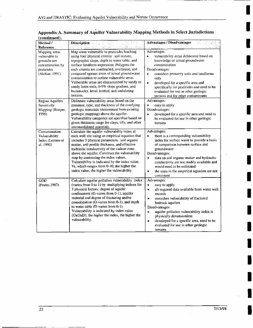
Appendix A. Summary of Aquifer Vulnerability Mapping Methods in Select Jurisdictions (continued). Method / Reference Mapping areas vulnerable to groundwater contamination by pesticides (McRae, 1991)

Regina Aquifers Sensitivity Mapping (Roeper, 1990)

Contamination Vulnerability

Map areas vulnerable to pesticides leaching using four physical criteria: soil texture, topographic slope, depth to water table, and surface landform expression. Polygons for cach critena are constructed, overlayed, and compared against areas of actual groundwater zontamination to outline vulnerable areas. Vulnerable areas are characterized by sandy or sandy loam soils, Q9% slope gradient, and hummocky, level, kettled, and undulating terrains. Delineate vulnerability areas based on the presence, type, and thickness of the overlying geologic materials (determined from existing geologic mapping) above the aquifer. Vulnerability categories are specified based on given thickness range for clays, tills, and other unconsolidated materials. Calculate the aquifer vulnerability index at each well site using an empirical equation that includes 3 physical parameters: soil organic matter, soil profile thickness, and effective hydraulic conductivity of the vadose zone above the aquifer. Construct the vulnerability map by contouring the index values. Vulnerability is indicated by the index value, Vi, which ranges from 0-10; the higher the index value, the higher the vulnerability.

Calculate aquifer pollution vulnerability index (varies from 0 to 1) by multiplying indices for 3 physical factors: degree of aquifer confinement (G-varies from 0-l), aquifer material and degree of fracturing and/or consolidation (0-varies from 0-1), and depth to water table (D-varies from 0-1). Vulnerability is indicated by index value (GxOxD); the higher the index, the higher the vulnerability.

Advantages / Disadvantages ~

Advantages: vulnerability areas delineated based on knowledge of actual groundwater contamination

Disadvantages: considers primarily soils and landforms only developed for a specific area and specifically for pesticides and need to be evaluated for use in other geologic terrains and for other contaminants

Advantages: easy to apply

Disadvantages: developed for a specific area and need to be evaluated for use in other geologic terrains

Advantages: there is a corresponding vulnerability index for surface water to provide a basis of comparison between surface and groundwater

data on soil organic matter and hydraulic conductivity are not readily available and would need to be estimated the units in the empirical equation are not consistent

Disadvantages:

Advantages: easy to apply all required data available from water well records considers vulnerability of fractured bedrock aquifers

Disadvantages: 0 aquifer pollution vulnerability index is

physically dimensionless developed for a specific area, need to be evaluated for use in other geologic terrains

22 7/13/98


. ..

AVI and DRASTIC: Evaluating Aquifer Vulnerability and Nitrate Occurrence I

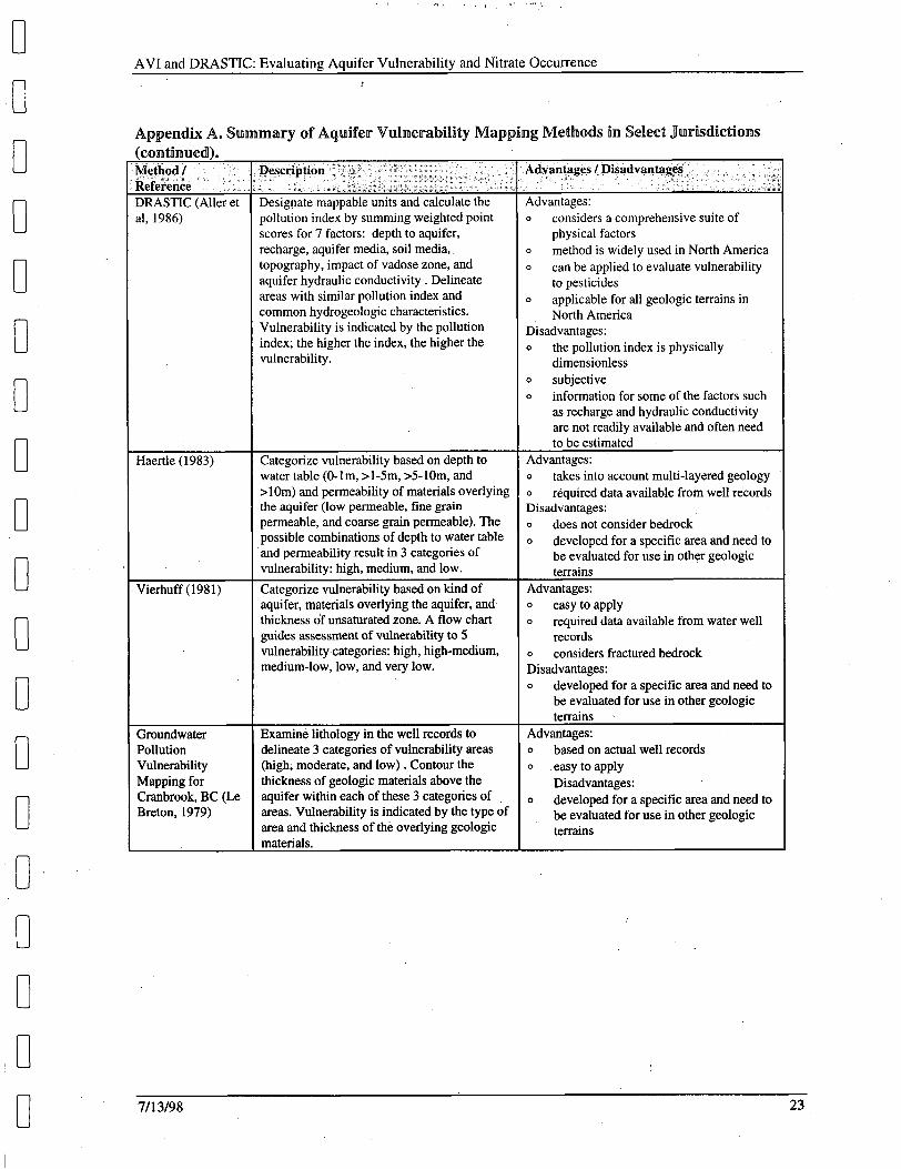
Appendix A. Summany of Aquifer Vunherability Mapping Methods iw Select Jlurisdictioms (CQwthUed) . Method / Reference DRASTIC (Aller et al, 1986)

Haertle (1983)

Vierhuff (1981)

Groundwater Pollution Vulnerability Mapping for Cranbrook, BC (Le Breton, 1979)

Description 1

Designate mappable units and calculate the pollution index by summing weighted point scores for 7 factors: depth to aquifer, recharge, aquifer media, soil media, topography, impact of vadose zone, and aquifer hydraulic conductivity . Delineate areas with similar pollution index and common hydrogeologic characteristics. Vulnerability is indicated by the pollution index; the higher the index, the higher the vulnerability.

Categorize vulnerability based on depth to water table (0-lm, >1-5m, >5-10m, and >lorn) and permeability of materials overlying the aquifer (low permeable, tine grain permeable, and coarse grain permeable). The possible combinations of depth to water table and permeability result in 3 categories of vulnerability: high, medium, and low. Categorize vulnerability based on kind of aquifer, materials overlying the aquifer, and thickness of unsaturated zone. A flow chart guides assessment of vulnerability to 5 vulnerability categories: high, high-medium, medium-low, low, and very low.

Examine lithology in the well records to delineate 3 categories of vulnerability areas (high; moderate, and low) . Contour the thickness of geologic materials above the aquifer within each of these 3 categories of areas. Vulnerability is indicated by the type of area and thickness of the overlying geologic materials.

7/13/98 23

4 dva

4dvantages: D

D

D

D

Disadvantages: o

o subjective 0

considers a comprehensive suite of physical factors method is widely used in North America can be applied to evaluate vulnerability to pesticides applicable for all geologic terrains in North America

the pollution index is physically dimensionless

information for some of the factors such as recharge and hydraulic conductivity are not readily available and often need to be estimated

takes into account multi-layered geology required data available from well records

Advantages: o

o

Disadvantages: o does not consider bedrock o developed for a specific area and need to

be evaluated for use in other geologic terrains

Advantages: 0 easy toapply 0 required data available from water well

records o considers fractured bedrock Disadvantages: o developed for a specific area and need to

be evaluated for use in other geologic terrains '

based on actual well records

Disadvantages: developed for a specific area and need to be evaluated for use in other geologic terrains

Advantages: 0

0 easy to apply

o

AVI and DRASTIC: Evaluating A w i f e r Vulnerabilitv and Nitrate Occurrence

Appendix * Well - No. -

1

2

3

4

18

20 21 25

26 29 33 36

37

42

45 48

49 54

57 58 59

61

66 67 68 70

71 76 77

B. AVI and DRASTIC Values for the Studv Wells.

screened @ 82-92'

N/A

Confined

Unconfined

Unconfined

I Unconfined NIA I

Confined Unconfined

N/A, Confined

4.276

3.697

0.825

-3.848

3.503

3.846 -5.203

AVI calculated for OB only; assume swl @ top of bedrock Aquifer interpreted to be sand @ 78-80; top 19' of sand assumed to be dry at well site Assume no resistance in 1 0 overburden above bedrock

AVI calculated for overburden above bedrock

AVI calculated for till to 8 4

I 18 I A I Confined

26 I C I Confined I I I thin sand layer at 107'- 1 1 0

26 I C I Confined I 4.102 I 19 I A I Unconfined I 2.109 I

Can't calculate AVI nor DRASTIC due to lack of lithology

NIA Confined 4.65 1 26 C Confined 3.899 Well completed at 110-120 26 C Confined 1.326 Confining layers from 0-61' +

NIA

15 A

Confined overburden above bedrock; AVI higher than for wells 48 & 49 due to 55' of overburden

Confined 4.535 Unconfined -0.932 Well screened from 95'-99'

Confined I 4.152 I Confined I 3.869 lTop of bedrock aquifer

assumed to be depth to I I bedrock

(adjacent wells) are similar; higher AVI for well 77 due

24 71 13/98


I 1 I I I I I I I

~1

I 1 1 I


84b NIA

87 15

88 15

89 15

f 94

95

96

-r 103

VI and DRASTIC Val

Unconfined

Unconfined

Unconfined

A I Unconfined Unconfined Unconfined Unconfined

A Unconfined Confined

C Confined

A Unconfined C Unconfined

3.825 High AVI but completed in hghly vulnerable aquifer with N03-N=4.19 mg/L; clay layer not likely extensive as wells 78 & 79 have low AVI numbers

.4.018 Although AVI number is low, well screen is at 99- 109', below silt layer (60- 70.5')

2.621 High AVI due to clay @ 44'- 49'

-2.8

Can't calculate AVI nor I DRASTIC, can't assume loverburden lithology

3.621 IHigh AVI due to clay @ 33'- 38'-

-2.307 Note that the duplicate log would give a much higher AVI number because of the description of "till" @ 15- 42.5'

3.478 High AVI due to till @ 29'- water table

-3.717

.4.371 -0.415 4.785 I Completed below

Abbdtsford-Sumas Aquifer (in Aldergrove Aquifer?)?

DRASTIC due to lack of lithology & can't assume

185 170 155

184

179 139

133

160

127

185 195 177 173 140 125

106

114 102

149 136

7/13/98 25


~ 108a

t q 113 115 35 119 35

123 72 124 NIA 7 134

V I and DRASTIC Values for the Study Wells (continued).

Vulnerability Unconfined Zlas5i fication

Aquifer Confined / AVI Comments . D R A

I Confined I 5.287 I I Unconfined 1 4.407 IAVI & DRASTIC for this C I 2 I 8

7 8 -

I I I I I

A Unconfined I -1.841 ICheck KRonneseths AVI I 5 I 9 I 7 I I / well location is for the West I I of Aldergrove aquifer

number for this well; AVI & DRASTIC calculated to uppermost aquifer, well tapping sand & gravel beneath blue clay @ 48-79', hence low N03-N (0.06 mgn) I I

A I Unconfined I -6 AVI undefined; zero 11019 resistance

Grandview aquifer (aq. no. 55)

C I Unconfined 3.662 Well completed into 9 9

I

southern, confined part of I

- 8

I I Ithe Hopington aquifer I I I A I Confined 1 3.702 I Well completed in the I 2 1 8 1 6

southern, confined part of the Hopington aquifer

C Confined 4.244 3 6 8 A I Unconfined 1-3.835 I

I Unconfined I 4.098 ICompleted into the 1 5 19 7 8 -

Abbotsford-Sumas aquifer? A Unconfined -3.631 7 8 8 C Can't calculate AVI nor 3 8

DRASTIC due to lack of lithology; AVI likely high &

I I C I Unconfined I 4.961 IAVI &DRASTIC calculatedl 9 18 I 8

for the deeper, confined

southern confined part of the

7 I 194

122 109

26 7/13/98

~ ~~

I I I

I I I I I I I I I 1 E I I I I

I I I I I I I

I I


ippen

135 136

138

139 140

141

142 146

147

148

150

151

153

155 156 157

158

159

160

161 162 -

iix B. AVI and DR Aquifer Aquifer

Classilication

NJA

41 A 41 A

41 A

33 C

33 C

NIA

32 C

27 C 27 C 27 C

58 C

51 C

35 A

8 A 8 A

GTIC Values for the Stud Wells (continuc Comments

unconfined

Confined 5 563 Confined 4.264 High AVI due to clay at 0 - 7

Confined 4.565 Located in the confined 5 22'

western part of the IHopington aquifer I

Confined 14.575 I 1 1

Unconfined

Confined

Confined

Beaver River aquifer

4.283 4.428 -0.361 Well record needs to be

revised; top of aquifer is 72', not 4 0

Nicomekl-Serpentine 5.331 Well completed into

1 2

I laquifer Confined I 4.986 IAVI calculated for 1

2

- 7 7 - -

uppermost WE4 zone; well screened @ 326-380'

4.59 Aquifer at 153', not 91' where sand is 2' thick. Completed in western confined part of Hopington aquifer

-4.652 -3.647

DRASnc

73 124

124

103 72

150

198 195

185

101

69

78

80

94 124 154

66

92

117

200 195 -

7/13/98 27



gravel 165 6 A Unconfined -3.932 9 9 8 168 6 A Unconfined -5.078 9 9 8

9 A Unconfined -6 AVI undefined; zero 10 9 8 171 resistance

is vulnerable but well is screened @ 80-84' & below

Unconfined

Unconfined

-2.029

-6

A

B

~

NIA

A Unconfined Confined

-4.141 4.761 5.1 13 e

de th to bedrock Confined

Unconfined

Unconfined

1.693

-0.962

-2.777

-3.476

A of this site may retlect the gravel w clay layer @ 15'-

SWL interpreted to be 24 , Unconfined average of well 190 and 165; AVI calculated for unconfined aquifer but well is completed below clay & till layers WT shallow therefore 5 aquifer is vulnerable but well is screened @ 95-100 & below CLAY @ 86-91' Lithology inferred from 10 surficial geology; assume SWL<=2m; AVI should be negative and DRASTIC should be high Lithology inferred from 10 surficial geology

Unconfined

A Unconfined -4.261

_((. A Unconfined

Unconfined Unconfined Unconfined Unconfined

-4.601

-3.371 -3.823 -3.736 -3.68

2.922

A A A A

C

198

199

Although AVI of aquifer is low, well is completed into sand and gravel below clayey layer The high AVI is due to the 1' clay layer, which may not be extensive High AVI due to clay @ 1'-

Unconfined

B Unconfined

Unconfined

4.068

-3.168 - B

28 7/13/98

I I I I I I I I I I I I iI I I I I I I

AVI and DRASTIC: Evaluating Acluifer Vulnerability and Nitrate Occurrence

ADDendix B. AVI and DRASTIC Values for the Studv Wells (continued).

202

203

204 205

206

208

209

210

21 1 212 213 215 216 217

218

219 220

22 1 222

223 224 225

226 227

228 229

113

107

139 109

102

1 04

179

96

135 116 107 106 178

167

91 133

107 145

117 86 180

175 180

165 185

7/13/98 29


~~

30 7/13/98


I I I I I I

264

265

266


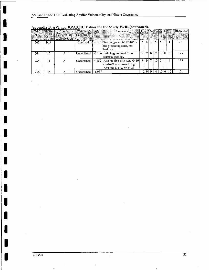
13 A Unconfined -3.756 Lithologyinferredfrom 7 9 8 9 10 8 10 193 surficial geology

(sw1)-47' is saturated; high AVI due to clay @ 8-25'

11 A Unconfined 4.152 Assumefinesiltysand @ 30 7 9 7 10 5 1 1 125

15 A Unconfined -1.937 2 9 9 4 10 6 10 151

I I I I I I I I I I I I

711 3/98 31

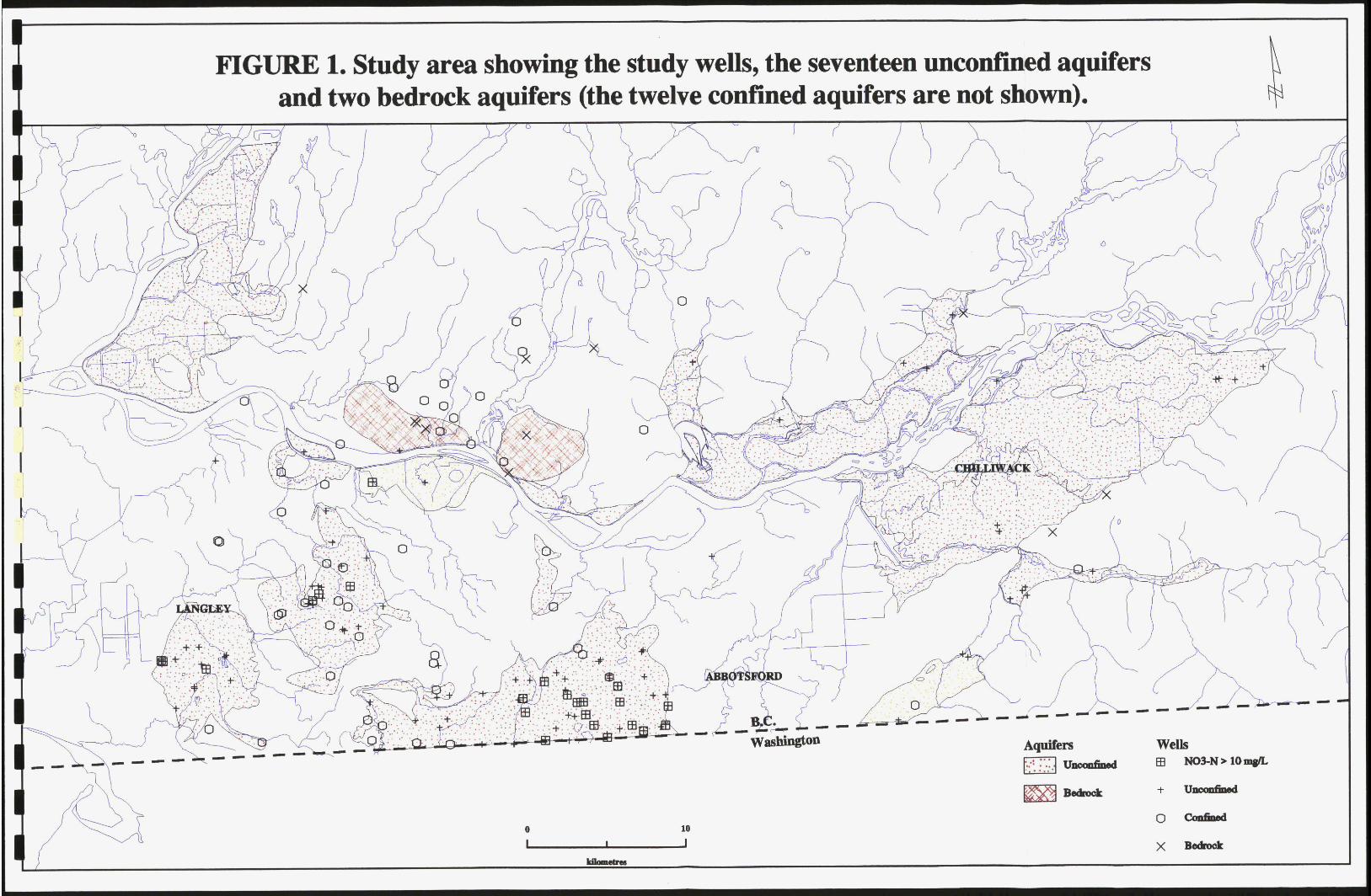
FIGURE 1. Study area showing the study wells, the seventeen unconfimed aquifers and two bedrock aquifers (the twelve confined aquifers are not shown).

Evaluating AVI and DRASTIC for Assessing Pollution ... · Aquifer Vulnerability and Nitrate...

Documents

Transcript of Evaluating AVI and DRASTIC for Assessing Pollution ... · Aquifer Vulnerability and Nitrate...