B Y

A L I N A Y O U N G

M I S S I S S I P P I W A T E R R E S O U R C E S C O N F E R E N C E

D E P A R T M E N T O F C I V I L E N G I N E E R I N G

M I S S I S S I P P I S TA T E , M I S S I S S I P P I

A P R I L 4 , 2 0 1 2

Evaluating a Vegetated Filter Strip in Agricultural Field

Outline Introduction Goals and Objectives Vegetated Filter Strip HSPF SUSTAIN Methodology Data Analysis Conclusions

Background The rising implementation of LIDs and BMPs in commercial, residential, and industrial areas has led to the need for the development of a useful hydrologic model The majority of BMP models that currently exist involve assessment based on pollutant efficiency rates (i.e. Hydrologic Simulation Program-FORTRAN) A newly released model by the United States Environmental Protection Agency (USEPA) entitled the System for Urban Stormwater Treatment and Analysis Integration (Alvi et al. 2009) includes a BMP component that predicts BMP effectiveness by using physical-based mathematical algorithms

Goals and Objectives The goal of this research is to perform a comparison of two water quality models (HSPF and SUSTAIN) to determine which model is more accurate at predicting BMP behavior. The objectives for this project were to answer the following questions:

1. How successful are HSPF and SUSTAIN at predicting BMP behavior? 2. Which BMP computational tool is more effective at predicting BMP behavior? 3. How adept is the BMP at reducing sediment and nutrient pollution? This research hopes to prove that the SUSTAIN BMP component will more accurately predict BMP effectives due to its physics-based mathematical processes than the HSPF-BMP percent removal rate computational model.

Vegetated Filter Strips The BMP selected for study in this research is a vegetated swale, or a vegetated filter strip (VFS) Vegetated filter strips are a “vegetated surface that [is] designed to treat sheet flow from adjacent surfaces. VFS function by slowing runoff velocities and filtering out sediment and other pollutants, and by providing some infiltration to underlying soils” (USEPA, 2006).

Background of HSPF HSPF is a semi-distributed, continuous simulation model with fixed user specified time steps, with its first release in 1980 by the USEPA. The most current version of it is called WinHSPF and is included in the Better Assessment Science Integrating Point and Nonpoint Sources (BASINS) package (USEPA, 2010) HSPF can model hydrology, sediments, and several water quality constituents Delineates each watershed into Hydrologic Response Units (HRUs) based on land use, soils, topography, and weather characteristics

HSPF’s BMPrac The Best Management Practices Editor (BMPrac) is an application module available for selection within HSPF once a UCI file has been created or opened in the program It allows the user to apply a BMP to a specific reach, identify the land uses affected by the BMP, define the percentage that the BMP affects the reach or land use, and define the removal efficiency rates for each pollutant (USEPA, 2009)

Background of SUSTAIN The increasing use of LIDs and BMPs in stormwater management plans led the USEPA to fund the development of a decision support system for LID and BMP selection and placements The goal of this system was to provide an assessment tool to aid in the development, evaluation, section, and placement of BMPs and LIDs based on cost and effectiveness Seven components for the system were identified: a framework manager, an ArcGIS interface, a watershed model, a BMP model, an optimization model, a post-processor, and a Microsoft Access database

SUSTAIN’s BMP Simulation ModuleProcess Option One Option Two

Flow Routing Stage-outflow using weir and/or orifice equations For swale: kinematics routing by solving the coupled continuity equation and Manning's equation.Infiltration Green-Ampt method Holtan-Lopez equationEvapotranspiration Constant evapotranspiration (ET) rate or monthly average value or daily values Potential ET using Harmon's methodPollutant Routing Completely mixed Continuously stirred tank reactor (CSTRs) in seriesPollutant Removal 1st order decay Kadlec and Knight's (1996) 1st order kinetic methodBuffer strip (sheet flow) flow routing Kinematics wave overland flow routingBuffer strip sediment trapping University of Kentucky sediment interception simulation method as applied in VFSMODBuffer strip (sheet flow) pollutant removal 1st order decay

The SUSTAIN BMP Simulation Module provides process-based simulation of flow and pollutant transport for a wide range of structural BMPs Users can select the preferred simulation method from either option depending on the available data, required level of detail, and the BMP being modeled

Methodologies

Site Selection and Characterization

ISCO at VFS Exit Rain Gauge ISCO at VFS Entrance The BMP chosen was a vegetated filter strip (VFS) located at South Farm Research Park at Mississippi State University in Starkville, Mississippi in Oktibbeha County The VFS was one of two that were installed in 2007 by Dr. Timothy Schauwecker to evaluate the effectiveness of common buttonbush (Cephalanthus occidentalis L. [Rubiceae]) in VFS(Avery & Schauwecker, 2008)

Site Selection and Characterization

(Germania Salazer, 2011)

Site Selection and Characterization

Site Selection and Characterization The VFS is located in a 82920 m2 Beef Unit Feedlot in the headwaters of the Noxubee River The goal of the VFS installation is to improve the quality of water runoff entering into the river from the Beef Unit Feedlot The area was 8m wide by 50m long and was enclosed with barbed wire fencing to protect it from surrounding cattle Water flows into the VFS both through two drainage pipes at its entrance and from sheet flow from the surrounding fields Check dams made of rip-rap were installed at the lower end of the VFS to slow down flow and aid in the growth of the 125 buttonbush plants that were installed

Instrumentation Two ISCO 3700 model auto-samplers; one sampler was installed at the entrance and one at the exit Samplers were held in place with steel rods and plastic-covered chains with locks Each sampler was able to hold 24 bottles at 500mL per bottle The samplers were programmed to collect composite samples of 100mL of water every 30mins for a total of 5 samples per bottle, or two and a half hours worth of data per bottle In order to conserve batteries the ISCOs were not left on full-time but were turned on at the beginning of each storm event. A TR-525 tipping rain gauge developed by Texas Instruments was installed at the site to obtain accurate rain data The rain gauge was used along with a CR1000 Data Logger which took measurements every .01mm of rain during storm events

Meteorological DataHilbun Hall

Study Site

HSPF has specific meteorological data requirements based on the intention of the user. Hourly precipitation, potential evapotranspiration, and air temperature were needed for the hydrology, sediments and nutrients modeled in this study A nearby weather station located at Hilbun Hall, the Geosciences Building at MSU was used for daily temperature and wind speed values for the Spring of 2011 (Mississippi State University , 2011).

Fertilizer Application The application of fertilizer in the Feedlots within the sub-basin occurred according the South Farm Forage Plan set out by the Mississippi State Extension Service ( Mississippi State University Extension Service, 2005).

Month Amount of Fertilizer Applied

Bermuda GrassApril 100lb of NitrogenJuly 50lb of NitrogenAnnual Rye GrassOctober 25lb of NitrogenNovember 25lb of Nitrogen

Soil Data Soil data such as hydrologic soil group, infiltration rates, and soil type was found using the National Resources Conservation Service (NRCS) Web Soil Survey (WSS) (NRCS, 2009). The soil series data listed on the NRCS is from the Soil Survey Geographic database (SSURGO). The site is comprised of six different soil types but primarily consists of poorly drained clay soils with high runoff potential.

Abbrev DescriptionHydrologic Soil Group

% Sand

% Silt

% Clay

Infiltration (in/hr)

Depth to Water Table

(in)Cp Catalpa silty clay loam C 17.8 52.2 30 0.06 -2.0 18-24Ho Houston silty clay D 8.3 50.2 41.5 0.0 to .0.06 48-72KlB2 Kipling silty clay loam (2-5% slopes) D 17.8 52.2 30 0.0 to .0.06 18-30KlC2 Kipling silty clay loam (5-8% slopes) D 17.8 52.2 30 0.0 to .0.06 18-30OlB2 Oktibbeha silty clay loam (2-5% slopes) D 18.7 47.8 33.5 0.0 to .0.06 < 80OlC2 Oktibbeha silty clay loam (5-8% slopes) D 18.7 47.8 33.5 0.0 to .0.06 < 80

Evaluation Methods VFS Efficiency Rate Nash-Sutcliffe Efficiency (NSE) Coefficient of Determination (R2) Relative Error (RE)

Data Results and Analysis

Data Analysis and Results This section delves into the presentation and analysis of the lab results of the samples obtained during the Spring of 2011 Data was taken for three storm events and analyzed for TSS, TKN, TP, and DP in the Civil and Environmental Engineering Laboratory at Mississippi State University

Lab Results: TSS

0.0200.0400.0600.0800.0

1000.01200.0

0 2.5 5 7.5 10 12.5

mg/

L

Duration - Hours

EntranceExit0.0500.01000.01500.02000.02500.03000.03500.04000.0

0 2.5 5 7.5 10 12.5 15 17.5 20 22.5 25 27.5 30

mg/

L

Duration - Hours

EntranceExit

TSS Results for 3/4/2011-3/5/2011 TSS Results for 3/8/2011-3/9/2011

Lab Results: TSS

TSS Results for 4/4/2011-4/5/20110.0

200.0400.0600.0800.0

1000.01200.0

0 2.5 5

mg/

L

Duration - Hours

EntranceFlume

Lab Results: Nutrients

0.1

1.0 0 2.5 5 7.5 10 12.5

mg/

L

Duration - Hours

TPDPTKNTKN - ExitTP - ExitDP - Exit0.1

1.0

10.0

0 2.5 5 7.5 10 12.5 15 17.5 20 22.5 25 27.5 30mg/

L

Duration - Hours

TPDPTKNTKN - ExitDP - ExitTP - Exit

Nutrient Results for 3/4/2011-3/5/2011 Nutrient Results for 3/8/2011-3/9/2011

Lab Results: Nutrients

0.1

1.0 0 2.5m

g/L

Duration - Hours

TPDPTKNTKN - ExitDP - ExitTP - Exit

Nutrient Results for 4/4/2011-4/5/2011

Lab Results: Nutrients

VFS Efficiency RatesEfficiency Rates

TSS TKN TP DP3/4/2011-3/5/2011 82.6 50.4 53.9 57.83/8/2011-3/9/2011 85.3 126.5 116.9 117.84/4/2011-4/5/2011 36.3 98.3 88.2 170.6Average 68.1 91.7 86.3 115.4

It is obvious that removal was not consistent for any pollutant over all three storm events. The VFS itself was most successful at removal of TSS.

HSPF Modeling Results Hydrology, sediments, and nutrients were modeled using HSPF Data for sediment and nutrients from the VFS at South Farm were used to calibrate the model from three storm events in the Spring of 2011 The main channel was treated as a single reach due to its small size; the total area of the watershed is 82920 m2 It was divided into four pervious segments and one impervious segment based on watershed characteristics and hydrologic soil groups

Segment Segment Name Hydrologic Soil Group Area (m2)PERLND 101 Pasture_HSG_D D 60270PERLND 102 Pasture_HSG_C C 16940PERLND 103 Road_HSG_D D 4230PERLND 104 Road_HSG_C C 730IMPLND 101 Roof D 730

HSPF Modeling Results The FTABLE for the model was computed using the FTABLE calculator on the USEPA’s website The FTABLE describes the channel characteristics of the site Two channels were created in the model: an open flow channel and a broad crested weir. This was done in order to take into account the behavior of the check dam at the exit of the BMP

Depth (m)

Area(m2)

Volume (m3)

Outflow1 (cms)

Outflow2 (cms)0 180 0 0 00.03 190 6.00 0.0008 00.61 490 203 0.186 00.67 520 233 0.225 0.3050.73 550 266 0.269 0.8630.79 580 301 0.344 1.585

HSPF Hydrology Results

00.0020.0040.0060.0080.010.0120.0140.0160.018

cms

EntranceExit

Observed flow data was not collected during the course of this study, yet it is still necessary to consider A look at the simulated flow was taken to understand the amount of water coming through the site both at its entrance and exit

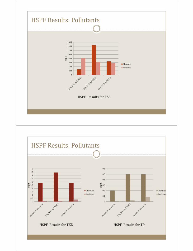
HSPF Results: Pollutants

02004006008001000120014001600

mg/

LObservedPredicted

HSPF Results for TSS

HSPF Results: Pollutants

00.10.20.30.40.50.6

mg/

L

ObservedPredicted

HSPF Results for TP00.51

1.522.533.544.55

mg/

L

ObservedPredicted

HSPF Results for TKN

HSPF Results: Pollutants

Pollutant R2 NSE RE (%)TSS 0.52 .22 5.2TKN 0.11 -0.17 2315TP 0.43 0.19 2842

HSPF appears to have greater success at sediment concentration prediction Discrepancy between observed and predicted nutrient values could be due to the limitation of only having data for three storm events. In addition nutrient processes would have greater accuracy if the more complex modeling routines mentioned earlier in the chapter could be used.

HSPF BMPrac Results The user selects the reach that the BMP is to be applied, the percentage that it affects the each land use segment, and the efficiency removal rates for each pollutant. A filter strip was created and applied to the reach. The area of the BMP (404 m2) divided by the area of each segment determined the percentage the BMP affected each land segment The efficiency rates used for application of the BMP in HSPF were the ones determined previously These rates as well as the percent that the BMP affected each model segment were input into the BMPrac Editor and applied to the reach

Segment Percent Effected by BMPPERLND 101 1.47PERLND 102 0.413PERLND 103 0.104PERLND 104 0.046IMPLND 101 0.018

HSPF BMPrac Results

0100200300400500600700800

mg/

LObservedPredicted

BMPrac Results for TSS

HSPF BMPrac Results

00.10.20.30.40.50.6

mg/

L

ObservedPredicted

BMPrac Results for TP00.51

1.522.533.544.55

mg/

L

ObservedPredicted

BMPrac Results for TKN

HSPF BMPrac Results Correlation between the observed data and the BMPrac data was not ideal Based on these values it seems that the BMPrac is not producing results that accurately describe what is actually occurring in the system. These results could possibly be improved with better calibration results for hydrology, sediment, and nutrient concentrations. Calibration parameters for the BMP itself would also make it easier to improve the performance of the model. The low degree that which the observed and predicted data agrees indicates that the BMPrac in HSPF is not ideal for BMP estimation.

Pollutant R2 NSE RE (%)TSS 0.28 -0.05 59758TKN 0.25 0.17 155TP 0 0 0

SUSTAIN BMP Module Results Time series for hydrology, sediments, and nutrients were exported from HSPF for use into SUSTAIN, opting for the external versus internal simulation option. This was chosen so that both BMP modules would have identical inputs in order to fairly asses their performance. The simulation of the VFS was conducted using training exercises provided with the program. A vast amount of parameters are required for modeling a VFS in SUSTAIN including dimension, substrate, growth index, water quality, sediment, and cost estimation When attempting to run SUSTAIN, the model produced an error and crashed

Conclusions

Findings Results show the VFS tends to be more successful at sediment concentration removal than at removal at nutrient concentration The nutrient levels in the system exceed the limits currently used by the MDEQ for TMDL studies proving that the water is greatly impaired There were difficulties during the model calibration due to limited available data and time constraints The addition of the VFS using HSPF’s BMP Practice Editor was relatively simple to use but was not an accurate representation of the physical processes occurring at the actual site Although SUSTAIN shows promise of being a useful and innovative modeling tool it still has several bugs and other issues that need to be resolved

Limitations and Further Research Lack of stream gauge Issues with the ISCO 3700 samplers led to the loss of data collection during storm events. A rain gauge was installed for the duration of the study and this was used in the model for precipitation data. As previously stated other meteorological data was acquired through a weather station located at the Mississippi State University campus. Although the station is merely a few miles away, the farm under examination is so small that this distance may affect the results. Ideally the soil infiltration rates and particles sizes would have been sampled in the field

Limitations and Further Research Installation of an ISCO at the second pipe entering the VFS could provide a closer look at the amount of pollutants entering the system. An attempt of model calibration and BMP simulation should be attempted again after at least a year’s worth of data has been collected If the VFS is still not removing pollutants in a desirable fashion after a year, perhaps it could be lengthened to try and increase its efficiency A wider channel at the entrance would also allow additional time for the pollutants to settle out before exiting the system. Nutrient simulation using the other routines (NITR and PHOS) would possibly increase accuracy of results A modeling attempt solely using SUSTAIN for flow, sediments, nutrients, and BMP simulation would be interesting to test SUSTAIN’s modeling capabilities.

Conclusions The goal of this research was the comparison of two BMP modeling programs and examines the effectiveness of BMPs to remove pollutants in a vegetated filter strip with a porous check dam Evaluation of HSPF versus SUSTAIN was unable to be completed due to SUSTAIN’s inability to successfully run the simulation, so it is still unclear whether a physics based BMP model would provide greater accuracy than an model like HSPF that uses efficiency rates Based on HSPF’s over prediction of pollutant removal, a physics based model still might produce better results but this cannot be stated with any certainty Hopefully further updates and developments to the SUSTAIN program will improve and promote its use and the use of BMPs in the future.

Questions?

AcknowledgementsThanks to all those at the Department of Civil and Environmental Engineering at Mississippi State University who provided much needed assistance, especially Dr. Jairo Diaz-Ramirez, Dr. William H. McAnally, Dr. James Martin, Dr. John Ramirez-Avila, Sandra Ortega-Achury, Joe Ivy, Matt Moran, David Bassi, and Natalie Sigsby. Thanks also to Dr. Tim Schauwecker and Wayne Wilkerson of the Department of Landscape Architecture.

References1. Arnold, Bingner, Harmel, Liew, & Veith. (2007). Modeling Evaluation Guidelines for Systematic Quantification Accuracy in Watershed Simulations. ASABE , 885-900.2. Atlanta Regional Comission . (2001, August). Geogria Stormwater Management Manual.Retrieved December 2009, from http://www.georgiastormwater.com/3. Avery, H., & Schauwecker, T. A. (2008). Agricultural BMP's, HSPF, and FarmLatis.4. Chapra, S. (1997). Surface Water Quality Modeling. WCB/McGraw-Hill.5. Mississippi State University . (2011). Weather Archives. Retrieved 2011, from Department of Geosciences: http://geosciences.msstate.edu/ftpdata/wx/data/6. Mississippi State University Extenstion Service. (2005, May 21). South Farm Forage Plan.Retrieved March 2011, from MSU Cares: http://msucares.com/livestock/beef/msusouthfarm2005.pdf 7. National Resource Conservation Service. (2009, 11 11). Web Soil Survey. Retrieved April 2011, from http://websoilsurvey.nrcs.usda.gov/app/HomePage.htm8. U.S. Environmental Protection Agency. (2010, January 13). Reducing Stormwater Costs through

Low Impact Development (LID) Strategies and Practices. Retrieved December 3, 2010, from Polluted Runoff (Nonpoint Source Pollution): http://www.epa.gov/owow/NPS/lid/costs07/9. U.S. Environmental Protection Agency. (2006, May 24). Vegetated Filter Strip. Retrieved February 5, 2011, from National Pollutant Discharge Elimination System: http://cfpub.epa.gov/npdes/stormwater/menuofbmps/index.cfm?action=browse&Rbutton=detail&bmp=76&minmeasure=510. U.S. Environmental Protection Agency. (2009, Dec 7). BASINS 4 Lectures, Data Sets, and Exercises: Lecture Two. Retrieved April 2010, from Training: http://water.epa.gov/scitech/datait/models/basins/training.cfm