EVALUATING A MODERN IN-MEMORY COLUMNAR DATA …
93
Lappeenranta University of Technology School of Business and Management Degree Program in Computer Science Bahman Javadi Isfahani EVALUATING A MODERN IN-MEMORY COLUMNAR DATA MANAGEMENT SYSTEM WITH A CONTEMPORARY OLTP WORKLOAD Examiners: Professor Ajantha Dahanayake Supervisors: Professor Ajantha Dahanayake Dr. Alexander Böhm
Transcript of EVALUATING A MODERN IN-MEMORY COLUMNAR DATA …

Lappeenranta University of Technology
School of Business and Management
Degree Program in Computer Science
Bahman Javadi Isfahani
EVALUATING A MODERN IN-MEMORY COLUMNAR DATA
MANAGEMENT SYSTEM WITH A CONTEMPORARY OLTP
WORKLOAD
Examiners: Professor Ajantha Dahanayake
Supervisors: Professor Ajantha Dahanayake
Dr. Alexander Böhm

ii
ABSTRACT
Lappeenranta University of Technology
School of Business and Management
Degree Program in Computer Science
Bahman Javadi Isfahani
Evaluating a modern in-memory columnar data management system with a
contemporary OLTP workload
Master’s Thesis
93 pages, 34 figures, 7 tables
Examiner: Professor Ajantha Dahanayake
Keywords: Column-oriented DBMS, column store, HTAP, IMDB, performance, SAP
HANA, SQLScript, TPC-E, workload breakdown
Due to the considerable differences between transactional and analytical workloads, a “one
size does not fit all” paradigm is typically applied to isolate transactional and analytical data
into separate database management systems. Even though the separation has its advantages,
it compromises real-time analytics. To blur boundaries between analytical and transactional
data management systems, hybrid transactional/analytical processing (HTAP) systems are
turned into reality. HTAP systems mostly rely on in-memory computation to present
profound performance. Also, columnar data layout has become popular specifically for
analytical use-cases.
In this thesis, a quantitative empirical research is conducted with the goal of evaluating the
performance of an HTAP system with a transactional workload. HANA (High-Performance
Analytic Appliance), an in-memory HTAP system, is used as the underlying data
management system for the research; HANA comes with two data stores: a columnar and a
iii
row data store. Firstly, the performance of HANA’s columnar store is compared with the
row store. To generate the required workload, an industry-grade transactional benchmark
(TPC-E) is implemented. Secondly, a profiling tool is employed to analyze primary cost
drivers of the HTAP system while running the benchmark. Finally, it is investigated how
optimal an HTAP-oriented stored procedure language (SQLScript) is for the transactional
workload. To investigate this matter, several transactions are designed on top of TPC-E
schema; the transactions then are implemented with and without using SQLScript iterative
constructs. The transactions are studied regarding the response time and growth rate.
The experiment shows that the row data store achieves 26% higher throughput compared to
its counterpart for the transactional workload. Furthermore, the profiling results demonstrate
that the transactional workload mainly breaks down into eight components of HANA
including query compilation and validation, data store access and predicate evaluation, index
access and join processing, memory management, sorting operation, data manipulation
language (DML) operations, network transfer and communication, and SQLScript
execution. Lastly, the experiment reveals that the native SQL set-based operations
outperform the iterative paradigm offered by SQLScript.

iv
ACKNOWLEDGEMENTS
First of all, I am deeply grateful toward my supervisors. I would like to show my greatest
appreciation to Prof. Ajantha Dahanayake for the invaluable guidance and advice she
provided me. I also cannot find the words to express my gratitude enough for Dr. Alexander
Böhm; I believe I have been fortunate to have such a patient, knowledgeable, and supportive
supervisor who extremely cared about my work.
I also want to thank all members of HANA performance team at SAP for their wonderful
help and collaboration. I owe many thanks to Mr. Lars Hoemke, Mr. Joachim Puhr, and Mr.
Hassan Hatefi.
Last but not the least, I would like to dedicate this thesis to my exceptional father Ahmad,
caring mother Ashraf, and beloved sister Yalda for their endless love, support, and
encouragement throughout my life. I love them with all my heart.

5
TABLE OF CONTENTS
1 INTRODUCTION ............................................................................................ 9
1.1 PROBLEM DESCRIPTION ...................................................................................... 9
1.2 RESEARCH QUESTIONS ...................................................................................... 11
1.3 RESEARCH METHODOLOGY ............................................................................... 11
1.4 STRUCTURE OF THE THESIS ................................................................................ 12
2 RELATED WORK ......................................................................................... 14
2.1 DATABASE MANAGEMENT SYSTEM ................................................................... 14
2.1.1 Memory Hierarchy ....................................................................................... 15 2.1.2 Evolution Toward In-Memory Databases ..................................................... 16
2.1.3 Key Enablers of In-Memory databases ......................................................... 17 2.1.3.1 Main Memory Cost Development ......................................................... 17
2.1.3.2 Shift Toward Multi-Core Paradigm ...................................................... 18 2.1.3.3 Impact of memory resident data ............................................................ 19
2.1.4 Memory Wall ............................................................................................... 22 2.1.4.1 NUMA ARCHITECTURE ................................................................... 22
2.1.4.2 Cache Efficiency .................................................................................. 23 2.1.4.3 Prefetching ........................................................................................... 24
2.2 HYBRID ANALYTICAL/TRANSACTIONAL PROCESSING SYSTEM ........................... 24
2.2.1 Online Transactional Processing Systems .................................................... 24 2.2.2 Online Analytical Processing Systems .......................................................... 26
2.2.3 Relational data layouts................................................................................. 29 2.2.4 Column-Oriented Data Layout ..................................................................... 31
2.2.5 Breaking the Wall Between Transaction and Analytical Processing ............. 32 2.3 OLTP WORKLOAD BENCHMARKS ............................................................ 34
2.3.1 TPC-C Benchmark ....................................................................................... 35 2.3.2 SD Benchmark ............................................................................................. 37
2.4 SAP HANA ..................................................................................................... 40
2.4.1 HANA for Analytical Workloads ................................................................... 40 2.4.2 HANA for Transactional Workloads ............................................................. 40
2.4.3 HANA for Mixed Workloads ......................................................................... 42 2.4.4 SAP HANA SQLSCRIPT .............................................................................. 44
2.4.4.1 SQLScript Data Extension .................................................................... 44 2.4.4.2 SQLScript Procedural Extension .......................................................... 45
2.4.4.3 SQLScript Functional Extension........................................................... 46 2.4.4.4 Creating and Calling Procedures ........................................................... 46
2.5 TPC-E BENCHMARK ......................................................................................... 49
2.5.1 TPC-E Transactions ..................................................................................... 50

6
2.5.2 TPC-E Required Isolation Levels ................................................................. 52
2.5.3 Scaling the Benchmark ................................................................................. 52 2.5.4 TPC-E Functional Components .................................................................... 54
3 TPC-E BENCHMARK IMPLEMENTATION FOR SAP HANA ..................... 55
3.1 DATA LOADER .................................................................................................. 56
3.2 COMMON FUNCTIONALITIES .............................................................................. 57
3.3 DRIVER ............................................................................................................ 58
3.4 TIER A.............................................................................................................. 60
4 EXPERIMENT ............................................................................................... 62
4.1 EXPERIMENT CONFIGURATION .......................................................................... 62
4.1.1 Database Management System ..................................................................... 62 4.1.2 Underlying Hardware .................................................................................. 63
4.2 THROUGHPUT EVALUATION .............................................................................. 63
4.2.1 Achieved Throughput and Response-times .................................................... 64
4.3 PROFILING RESULTS ......................................................................................... 67
4.3.1 Workload Decomposition ............................................................................. 69 4.3.2 Checkpointing and Recovery ........................................................................ 72
4.4 SQLSCRIPT EVALUATION FOR OLTP WORKLOAD ............................................. 75
5 CONCLUSION ............................................................................................... 81
5.1 SCOPE AND BACKGROUND ................................................................................ 81
5.2 MAIN FINDINGS ................................................................................................ 82
5.3 FUTURE WORK ................................................................................................. 84
6 LIST OF TABLES .......................................................................................... 86
7 LIST OF FIGURES ........................................................................................ 87
8 REFERENCES ............................................................................................... 88

7
LIST OF SYMBOLS AND ABBREVIATIONS
ACID Atomicity, Consistency, Isolation, Durability
BI Business Intelligence
BCNF Boyce-Codd Normal Form
CE Customer Emulator
CPU Central Processing Unit
DB Database
DBMS Database Management System
DM Data Maintenance
DML Data Manipulation Language
DRAM Dynamic RAM
DRDB Disk-resident Database
DW Data Warehouse
DWH Data Warehouse
ETL Extract, Transform, Load
ER Entity Relationship
ERP Enterprise Resource Planning
GB Gigabyte
HANA High-Performance Analytic Appliance
HTAP Hybrid Analytical/Transactional Processing
IMDB In-memory Database
ITD Initial Trade Days
KB Kilobyte
MEE Market Exchange Emulator
MMDB Main-memory Database
MOLAP Multidimensional Online Analytical Processing
MVCC Multi-Version Concurrency Control
ODBC Open Database Connectivity
OLAP Online Analytical Processing
OLTP Online Transactional Processing
OS Operating System

8
NUMA Non-Uniform Memory Access
NVRAM Non-volatile RAM
PP Production Planning
PL/SQL Procedural Language/Structured Query Language
QPI Quick Path Interconnect
RAM Random Access Memory
RLE Run Length Encoding
ROLAP Relational Online Analytical Processing
SD Sales and Distribution
SF Scale Factor
SIMD Single Instruction/Multiple Data
SMP Symmetric Multiprocessing
SQL Structured Query Language
SRAM Static RAM
SUT System Under Test
T-SQL Transact-Structured Query Language
TB Terabyte
TCO Total Cost of Ownership
TPC Transaction Processing Performance Council
TSX Transactional Synchronization Extensions
VM Virtual Memory

9
1 INTRODUCTION
1.1 Problem Description
Nowadays data is at the heart of organizations; in fact, data is crucial for businesses not only
to operate their businesses but also to make sound decisions in a competitive market.
Consequently, regardless of their sizes and business domains companies are exploiting
database management systems (DBMSs) as the backbone to store and manage their data.
Data-intensive applications can be classified into two broad categories: online transactional
processing (OLTP) and online analytical processing (OLAP), and each one exhibit specific
characteristics and requirements [1]. In OLTP systems, such as enterprise resource planning
(ERP), DBMSs have to cope with a massive number of concurrent, short-lived transactions,
which are usually simple (e.g., displaying a sale order for a single customer) while
demanding milli-seconds response times. On the other hand, OLAP workloads are
characterized by comparatively low volumes of yet complex and long-running queries.
Due to substantial differences between OLTP and OLAP workloads, different optimizations
are applied in database management systems. To put it another way, the architecture of some
database systems has been highly optimized for transaction processing like Microsoft SQL
Server Hekaton [2] and H-Store [3] ; that of the others has been calibrated in conformity
with analytical workload requirements (i.e., data warehouses) such as MonetDB [4] and HP
Vertica [5]. Besides the optimizations, the data management systems have utilized disparate
data layouts for OLTP and OLAP data. For instance, analytical data are traditionally
consolidated into multi-dimensional data models such as star and snowflake, whereas the
transactional data is mostly modeled using highly normalized relations [6]. One approach to
serving the different requirements is separating the systems and running extract, transform,
load (ETL) process to load operational data from OLTP systems to the OLAP ones. The
periodical ETL process brings about four significant disadvantages [7]. Firstly, the ETL
process is time-consuming and of high complexity. Secondly, the process compromises real-
time analytics by relying on historical data. Also, acquiring two separate solutions increases
the total cost of ownership (TCO). Last but not the least, keeping data inside two distinct
systems leads to data redundancy.
10
In a conventional relational DBMS, data is stored in a row-wise manner meaning that records
are stored sequentially. Copeland and Khoshafian [8] introduced an alternative approach to
store the relations in the 1980s; the proposed data storage named columnar (also called
column-oriented), keeps relations by columns as opposed to rows of data. Advantages of the
columnar storage are fourfold compared to the row-oriented layout [9]. To start with,
uniformity of the data stored as columns will pave the way for far better compression rates
and space efficiency. Secondly, the columnar storage architecture enables extensive data
parallelism. Moreover, it provides better performance for aggregations; aggregation is an
essential operation for analytical queries. Finally, fewer data should be scanned in the
columnar storage if queries access a few attributes. Recently, using columnar databases is a
prominent approach for analytics gradually replacing the multi-dimensional data models [7].
However, it is lively discussed that the storage does not meet OLTP requirements due to two
main reasons [10, 11]:
• OLTP queries mostly operate upon more than one relation field. Thus, accessing
multiple fields is more scan-friendly in the row-oriented approach.
• Maintaining columnar storage in an update-intensive environment is expensive.
Besides the popularity of the columnar storage, in-memory database systems (IMDBs, also
called main-memory database systems or MMDBs) are becoming more widespread. In the
past decade, we have experienced a plummeting cost of dynamic ram (DRAM) modules and
an ever-growing DRAMs’ capacities Hence, in-memory database systems have turned into
reality. The in-memory data management systems eliminate disk latencies and operate upon
the data loaded into main memory. The systems present profound performance
improvements as well as a foundation to satisfy new business requirements. [6]
To blur boundaries between analytical and transactional data management systems, some
disruptive approaches have been taken toward building a single data management system
capable of processing a mixture of both analytical and transactional workloads. The systems
are so-called hybrid transactional/analytical processing (HTAP). Presently, a number of
HTAP systems are available in the market including SAP HANA [12], HyPer [13], and
VoltDB [14]. For instance, SAP (a multinational software company headquartered in
Germany) has embraced the advantages of the columnar storage plus the strengths of in-

11
memory data management into a single solution, HANA (HANA stands for High-
Performance Analytics Appliance). SAP HANA, an in-memory DBMS initially designed
for purely analytical workloads, has evolved to a system which supports mixed workloads
on a columnar representation; the system can serve enormous enterprise resource planning
(ERP) installations with 5 million queries per hour and more than 50K concurrent users [12].
1.2 Research Questions
There is no consensus on the efficiency of having a single data management system which
can serve both analytical and transactional workloads. On the one hand, the approach has
been overtly questioned by several studies [11, 10]. For instance, M. Stonebraker and U.
Çetintemel [11] have argued that the hybrid approach is a marketing fiction. On the other
hand, some HTAP systems such as SAP HANA are widely used as explained in the previous
section. In fact, HANA has been designed to combine OLAP and OLTP workloads and the
underlying data set based on columnar representation [9].
This study aims to answer the following research questions using SAP HANA as the
underlying system.
• RQ1) How does an in-memory columnar HTAP perform with OLTP workload?
• RQ2) How does OLTP workloads breakdown into major components of an HTAP
system?
• RQ3) How optimal an HTAP-oriented stored procedure language like HANA
SQLScript is (see section 2.4.4) for OLTP workloads?
1.3 Research Methodology
This research consists of two central actions: a systematic literature study and a quantitative
empirical research. The literature study covers:
• In-memory databases
• HTAP systems
• OLTP benchmarks
• SAP HANA.

12
The empirical study demands two major requirements.
1. An enterprise HTAP system supporting both row and columnar stores: SAP HANA
is the data management system used in the thesis.
2. Implementing an industry-grade OLTP benchmark: TPC-E benchmark, an OLTP
benchmark published by Transaction Processing Performance Council (TPC), is used
for in the thesis. The benchmark is open source; it is designed to represent
requirements of a contemporary OLTP system, and widely recognized by the
database community.
After the implementation of the benchmark, it is run against both the data-storages to
understand to what extent they differ regarding throughput. Then, profiling tools are used to
understand how the OLTP workload decomposes into different components in SAP HANA.
Finally, the study drills down into the mechanics of SQLScript language to analyze its
efficiency for OLTP workloads.
1.4 Structure of the thesis
This subsection contains a short description of the structure of this thesis. The thesis is
divided into six chapters. Chapter 2 of the thesis incorporate the literature study. Section 2.1
explores in-memory databases. The purpose of this section is to understand what are
enablers, inner mechanics, and challenges with in-memory databases. Then, HTAP systems
are investigated in section 2.2. The section 2.2 aims first to understand the main requirements
of OLTP and OLAP systems. It is then explained how columnar and row-oriented databases
correspond to the requirements. The section 2.2.5 finally wraps how a hybrid system can
break the gap between transactional and analytical processing.
Afterwards, OLTP benchmarks are studied in section 2.3. A proprietary and an open-source
benchmark have been reviewed in this chapter. The chapter presents how the benchmarks
portray activities of OLTP systems.
Section 2.4 studies SAP HANA to understand how an HTAP system is designed.
Understanding internal mechanisms of HANA then aids analyzing the experiment results.

13
An overview of SQLScript, a stored procedure language provided by SAP, is also provided
since in the experiment transactions are implemented using the scripting language.
The TPC-E benchmark is inspected in section 2.5. The study helps the implementation and
the analyzing stages. It also depicts how OLTP requirements have changed over the course
of time by comparing the benchmark with its predecessor (i.e., TPC-C).
Chapter 3 explains the implementation of the benchmark used for the experiment.
Technologies and the architectural designs applied to the implementation are also discussed
in the section.
Finally, Chapters 4 and 5 demonstrate the results of the experiment and the main findings.
The chapters also point out the limitations of the current work and the opportunities for future
research.

14
2 RELATED WORK
2.1 Database Management System
A database (DB) is a set of data being organized in a meaningful way and accessible in
different logical orders [15]. Furthermore, a database management system is a combination
of a DB and a management system (MS). The primary objective of the management system
is to aid data store and retrieval with efficiency and convenience [1]. DBMS can be regarded
as an intermediary between entities who desire accessing a database (i.e., applications or
end-users), and the actual physical data.
Database systems have been widely used over the course of the last five decades in
multitudes of different applications including enterprise information systems, banking,
education, telecommunication, and many more. Before database management systems are
introduced, organizations mostly stored their organizational information in so-called flat
files. Leveraging the database management systems is advantageous in several aspects
compared to the file-processing systems. To begin with, the central data management system
circumvents problems related to data redundancy and inconsistency. Moreover, the DBMS
offers data independence by applying different levels of abstraction. What’s more, using
systems ensures ACID (Atomicity, Consistency, Isolation, and Durability) properties in
transaction level. Finally, the systems enable data security by applying access control
constraints. [1]
Databases utilize a collection of conceptual tools for describing data, relationships among
them, data semantics, and consistency constraints. The collection is called data model and is
the underlying structure of a database. The data models can be classified into several
different categories such as relational and object-based as well as some semi-structured and
unstructured data models. Among the data models, the relational is the most widely used.
The relational model takes advantage of a collection of tables to represent data and the
relationships between the data. The tables in the model are known as relations, and each
relation consists of multiple columns with unique names. IBM developed the first
experimental prototype for a relational DBMS as “System R” in the late 1970s. The focus

15
of this paper is on Relational DBMS (RDBMS) which is referred as DBMS for the sake of
consistency. [1]
2.1.1 Memory Hierarchy
As can be seen in Figure 1, a memory system is a hierarchy of storage devices. Each device
has different costs, capacities, and access times. There is one specific characteristic in the
hierarchy: the higher in the pyramid, the higher performance will be achieved. It is worth
mentioning that the higher performance compromises the costs. [7]
Figure 1 Conceptual view of memory hierarchy [7]
The CPU caches are made from static ram (SRAM) cells which provide data remanence as
long as power supplied and are usually built out of four to six transistors [7]. In contrast,
main memory is typically built of dynamic ram (DRAM) cells that are constructed using
much simpler structure (i.e., a transistor and a capacitor). The more straightforward structure
of DRAM cells makes it more economical compared to SRAM. However, the capacitor
discharges over time; hence, DRAM chips should be refreshed periodically [16]. The
charging and discharging of the capacitor limits the speed of DRAM cells. The hard disk is
at the very bottom of the view. Even though hard disks offer massive capacities at
economical prices, they are attributed to high access and read times.
Latency is a measurement to grasp how different storage media act in terms of performance.
The latency is the time delay to load the data from the storage device until it is available in
one of CPU registers [6]. While an L1 CPU cache reference (modern processors have
multiple levels of cache including L1, L2, and L3) takes 0.5 ns, accessing the main memory
reference takes 100 ns and a simple disk access takes 10 ms [7]. In the next section, it is

16
explained how the significant difference in latency between the hard disk and main memory
has led to building a new generation of database management systems.
2.1.2 Evolution Toward In-Memory Databases
Enterprise applications today demand more stringent throughput and response time
requirements than ever before. Also, companies have become more data-driven and require
to process ever-growing enormous data volumes to support their management decisions.
Consequently, it is a must that data management systems meet the imposed requirements
and constraints. Conventional disk-resident database systems (DRDBs) use disks as the
primary storage and bring data into main memory as needed. This frequent disk access
introduces a main bottleneck for the systems since disk input/output (I/O) could cause orders
of magnitudes higher latency compared to main memory [6].
To address the disk I/O bottleneck, in-memory database systems (IMDBs, also called main
memory database systems or MMDBs) are adapted as a new breed of database management
systems. The database systems place data inside main memory and operate upon the data
kept in the memory. The approach not only provides a profound performance improvement
but also presents a foundation to satisfy new business requirements. Figure 2 depicts the
advantage of using an in-memory database engine for a single primary key fetch and single
row update based on the primary key in solidDB, an in-memory solution offered by IBM. In
IMDBs, the role of disks could be left as persistent storage [6, 17].
Figure 2 Advantage of using in-memory data management for a single fetch and a single row update [18]
To alleviate the disk I/O barrier, disk-resident database systems have extensively applied
caching mechanisms to keep frequently accessed data in main memory. According to [17,
17
19], there are three primary differences between an IMDB and a DRDB with a huge cache.
First, a DRDB still needs a buffer pool manager even when the data being accessed is already
cached in main memory; accessing data through a buffer manager brings about overhead. A
study by Lehman et al. [19] suggests that using the buffer manager increases execution times
up to 40% even the database is cached in memory. Secondly, the related techniques
developed for DRDBs are optimized under the assumption of disk I/O as the main cost of
the system [20]. On the other hand, in designing and optimizing in-memory database systems
achieving high performance on memory-bound data is of concern. Thirdly, using a main
memory cache strategy still requires a buffer manager to compute the corresponding disk
address of each requested tuple and check the existence of the computed address data in
main memory while in IMDB data are accessed directly by referring to their memory address
[17]. In other words, logical addressing will be replaced by memory-based addressing.
2.1.3 Key Enablers of In-Memory databases
IMDB is not a brand-new notion and has been studied as early as the 1980s [17, 21];
however, there are two dominant reasons that a wide range of IMDB solutions have turned
into reality. The reasons are studied in the two next subsections.
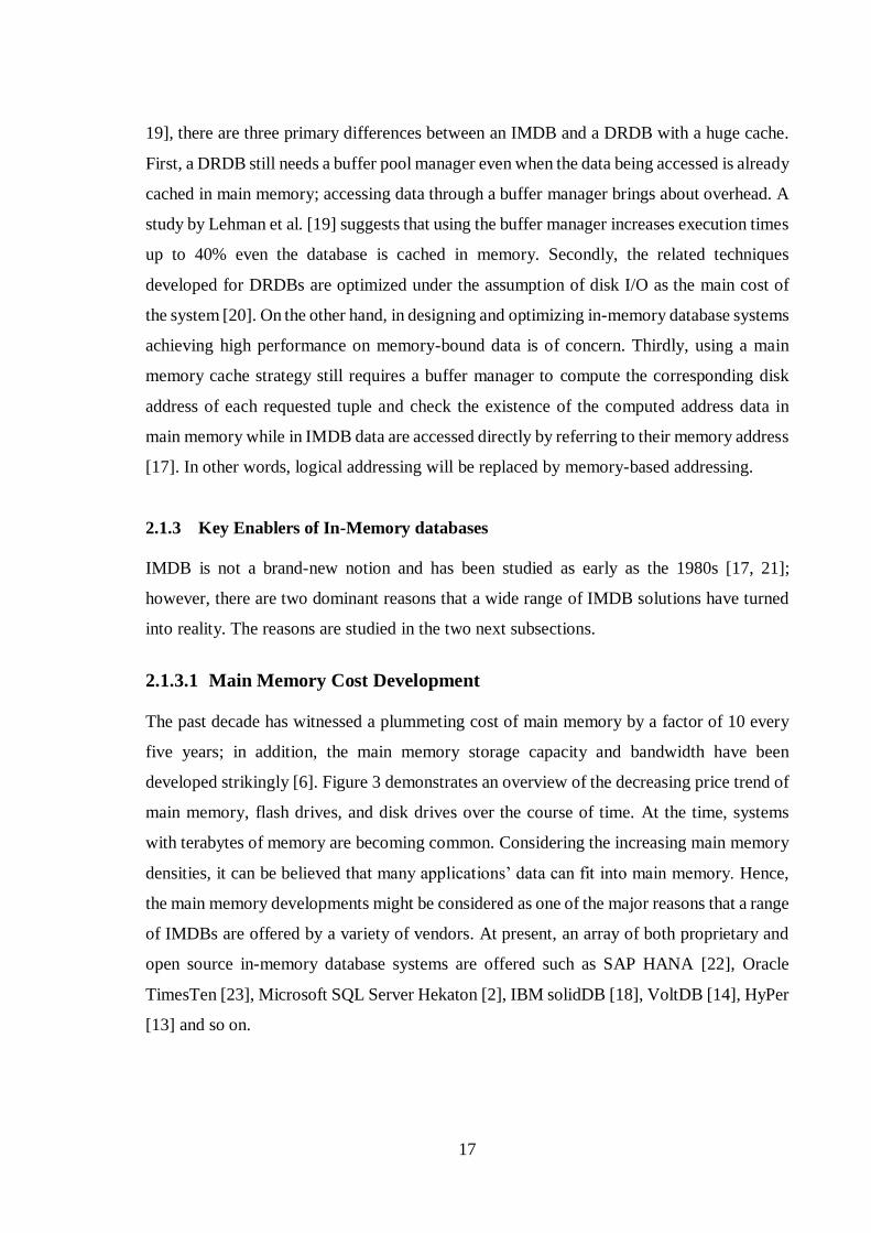
2.1.3.1 Main Memory Cost Development
The past decade has witnessed a plummeting cost of main memory by a factor of 10 every
five years; in addition, the main memory storage capacity and bandwidth have been
developed strikingly [6]. Figure 3 demonstrates an overview of the decreasing price trend of
main memory, flash drives, and disk drives over the course of time. At the time, systems
with terabytes of memory are becoming common. Considering the increasing main memory
densities, it can be believed that many applications’ data can fit into main memory. Hence,
the main memory developments might be considered as one of the major reasons that a range
of IMDBs are offered by a variety of vendors. At present, an array of both proprietary and
open source in-memory database systems are offered such as SAP HANA [22], Oracle
TimesTen [23], Microsoft SQL Server Hekaton [2], IBM solidDB [18], VoltDB [14], HyPer
[13] and so on.
18
Figure 3 Storage price development [6]
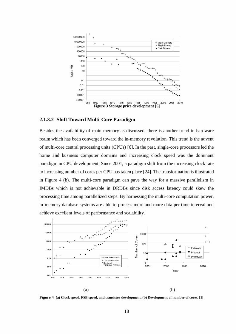
2.1.3.2 Shift Toward Multi-Core Paradigm
Besides the availability of main memory as discussed, there is another trend in hardware
realm which has been converged toward the in-memory revolution. This trend is the advent
of multi-core central processing units (CPUs) [6]. In the past, single-core processors led the
home and business computer domains and increasing clock speed was the dominant
paradigm in CPU development. Since 2001, a paradigm shift from the increasing clock rate
to increasing number of cores per CPU has taken place [24]. The transformation is illustrated
in Figure 4 (b). The multi-core paradigm can pave the way for a massive parallelism in
IMDBs which is not achievable in DRDBs since disk access latency could skew the
processing time among parallelized steps. By harnessing the multi-core computation power,
in-memory database systems are able to process more and more data per time interval and
achieve excellent levels of performance and scalability.
(a) (b)
Figure 4 (a) Clock speed, FSB speed, and transistor development, (b) Development of number of cores. [1]
1
10
100
1000
2001 2006 2011 2016 Year
Estimate Product Prototype

19
2.1.3.3 Impact of memory resident data
As explained in Section 2.1.2, IMDBs provide a profound implication on performance
comparing to DRDBs. However, such an excellent performance cannot be gained merely by
placing data in the memory. Indeed, it demands specific optimizations to maximize the
performance. In this section, the critical issues and optimizations required while building a
main-memory database system are briefly introduced. The challenges and choices are
discussed based on the following concepts.
1. Data storage: Unlike the disk-resident DBMSs in which on-disk formats constrain
data layout, in-memory database management systems are more flexible in
leveraging formats that could gain better performance and design goals [17]. To
illustrate, clustering records per a primary key index is often used for storing data in
the disk-resident systems [25]. However, in main memory databases, sets of pointers
to data values could represent relational tuples [17]. As it is discussed in [17], taking
advantage of the pointer following sequences for the data representation is twofold.
First, in cases there are variables appeared multiple times in the database, pointers
could refer to a single stored value and save space [26, 27]. Secondly, it streamlines
handing variable-length fields because the fields are represented as a pointer into a
heap [28, 29].
2. Buffer Management: DRDBs traditionally exploit buffer managers to hide disk
access latency. Upon receiving a block access, the buffer manager seeks inside an
array of page objects (called buffer pool) and returns the corresponding main
memory address providing that the block is found in the buffer pool. Otherwise, it
reads the block from disk into the buffer pool. The buffer manager should use a
replacement strategy like Least Recently Used (LRU) in cases that the pool is full.
In addition, using the buffer manager requires synchronization techniques to
synchronize data between disk and the buffer pool. Even though the buffering could
provide a performance gain, it has some expenses like calculating the addresses and
high paging overheads. On the other hand, IMDBs are free from the buffer
management overheads since all operating data is kept inside main memory. [19]
3. Indexing structure: It has been discussed that traditional data structures like
balanced binary search trees are not efficient for main memory databases running on

20
a modern hardware [30, 17, 31]. Firstly, the traditional data structures do not
optimally exploit on-CPU caches (are not cache-efficient) [30]. Secondly, main
memory trees do not require short bushy structures because traversing deeper trees
is much faster in main memory comparing to disk [17]. Hence, several new indexing
structures have been designed and proposed for use in main memory like Bw-Tree
[32], T-Tree [31] and ART [30]. According to [25], multi-core scalability and
NUMA-awareness (NUMA stands for Non-Uniform Memory Access) are also of
high importance in designing indexing methods since indexing structures could
provide a foundation for parallelism.
4. Concurrency control: It is argued that in an IMDB, lock contention may not be as
significant as in a DRDB since transactions are likely to be completed more quickly
and locks will not be held as long [17]. Hence, choosing small locking granules such
as fields or records might not be effective in reducing lock contentions; it is suggested
that large lock granules (e.g., relations) are more efficient for memory resident data
[28]. It is also proposed that the objects in memory can contain lock information to
represent their lock status instead of using hash tables containing entries for the
locked objects [17]. Besides the mentioned concurrency control optimizations, most
modern systems are shifting from pessimistic two-phase locking mechanism to the
optimistic ones that ideally never block readers while still supporting high ANSI
isolation levels like serializability [25]. Also, using latch-free data structures is
another approach that has been adapted for achieving high levels of concurrency [2].
5. Query processing and compilation: Most conventional database systems translate
a given query into algebraic expressions. The iterator (also called Volcano-style
processing) is a traditional method for executing the algebraic expressions and
producing query results; each plan operator yields tuple streams that are iterable by
using the next function of the operator [33]. While the iterator model is acceptable
in disk-resident database systems, it shows poor performance on in-memory database
systems due to frequent instruction mispredictions and lack of locality [34]. The
issues have led several modern main memory systems to depart from the algebraic
operator model to query compilation strategies which compile queries and stored
procedures into machine codes [34].
21
6. Clustering and distribution: There are two dominant architectural choices in
handling the intensifying workloads and volumes of data in IMDBs: vertical scaling
and horizontal scaling [25]. Scale-up (i.e., vertical scaling) is the capability of
handling the growing workloads by adding resources into a given machine while in
scale-out (i.e., horizontal scaling) the increasing workload would be dealt with by
adding new machines to the system [6]. Systems like H-Store/VoltDB are built from
the square one to scale-out by running on a cluster of shared-nothing machines [25].
On the other hand, systems like Hekaton are initially built to be deployed using a
shared-everything architecture and scale up to larger multi-socket machines with
massive amounts of resources [25]. Shared-everything within a database node is any
deployment in which a single database node manages all available resources
whereas, in shared-nothing deployment, several independent instances process the
workload [35]. There are also some systems such as SAP HANA which leverage
both approaches to enable scalability according to the requirements [36].
7. Durability and recovery: IMDBs require having a persistent copy and a log of
transaction activities to protect against crashes and power loss [17]. The log should
be kept in a non-volatile storage, and each transaction’s activities must be recorded
in the log [37]. Logging can affect response times and throughput and threatens to
undermine the achieved performance advantages of memory resident data since each
transaction demands a disk operation. To mitigate the problem, several solutions
have been proposed [21, 38, 39, 29]. The first proposed solution is using a stable
main memory for keeping a portion of the log. In this approach, each transaction
commits by writing its log information in the stable memory, and a special process
is required to replicate the log information to the log disks. The approach will
alleviate the response times, yet the log bottleneck will not be remedied. The second
proposed solution includes using the notion of pre-committed transactions. In this
scheme, the transaction management system places a commit record into the log
buffer whenever a transaction is ready to complete. The transaction does not wait for
the commit record to be propagated to disk. The solution might reduce the blocking
delays of other concurrent transactions. Finally, group commits have been introduced
to amortize the cost of the log bottleneck. In the group committing, records of
multiple transaction logs can be accumulated in the memory before being flushed to

22
disk. The group committing will improve application response times and transaction
throughput. It is worth mentioning that many modern main-memory systems have
employed new durability methods since the row-oriented log-ahead mechanisms
bring about performance overheads [25]. For example, a study has shown 1.5X
higher throughput by applying a command-logging technique which only records
executed transactions [40]. The technique facilitates the recovery by replaying the
logged commands on a consistent checkpoint.
2.1.4 Memory Wall
As explained in Section 2.1.2, the increasing availability of main memory and the paradigm
shift toward many-core processors are the two major trends which can profoundly affect in-
memory data management systems. The proliferations give rise to new possibilities yet new
challenges. Processor caches are connected to main memory through a front side bus (FSB).
In the past decades, advances in processing speed have outpaced advances in main memory
latency [41]. Thus, CPU stalls while loading data from main memory to CPU cache has
become a new bottleneck. The widening gap between the processing speed and the main
memory access is widely known as the ”memory wall” [41]. In the following subsections,
we study different mechanisms to hide the memory wall.
2.1.4.1 NUMA ARCHITECTURE
To take advantage of the increasing process capacity, FSB performance should keep up with
the exponential growth of the processing power. Unfortunately, during the past decade, FSB
performance has not been developed conforming with processing power as shown in Figure
4(a). In traditional symmetric multiprocessing (SMP) architecture, all processors are
connected to the main memory via a single bus. Consequently, bus contention and
maintaining cache coherency will intensify the situation. To partially circumvent this
problem, non-uniform memory architectures (NUMA) have become the de-facto
architecture of new generation of enterprise servers. NUMA is a new trend in hardware
toward breaking a single system bus into multiple busses, each serving a group of processors.
[6]
23
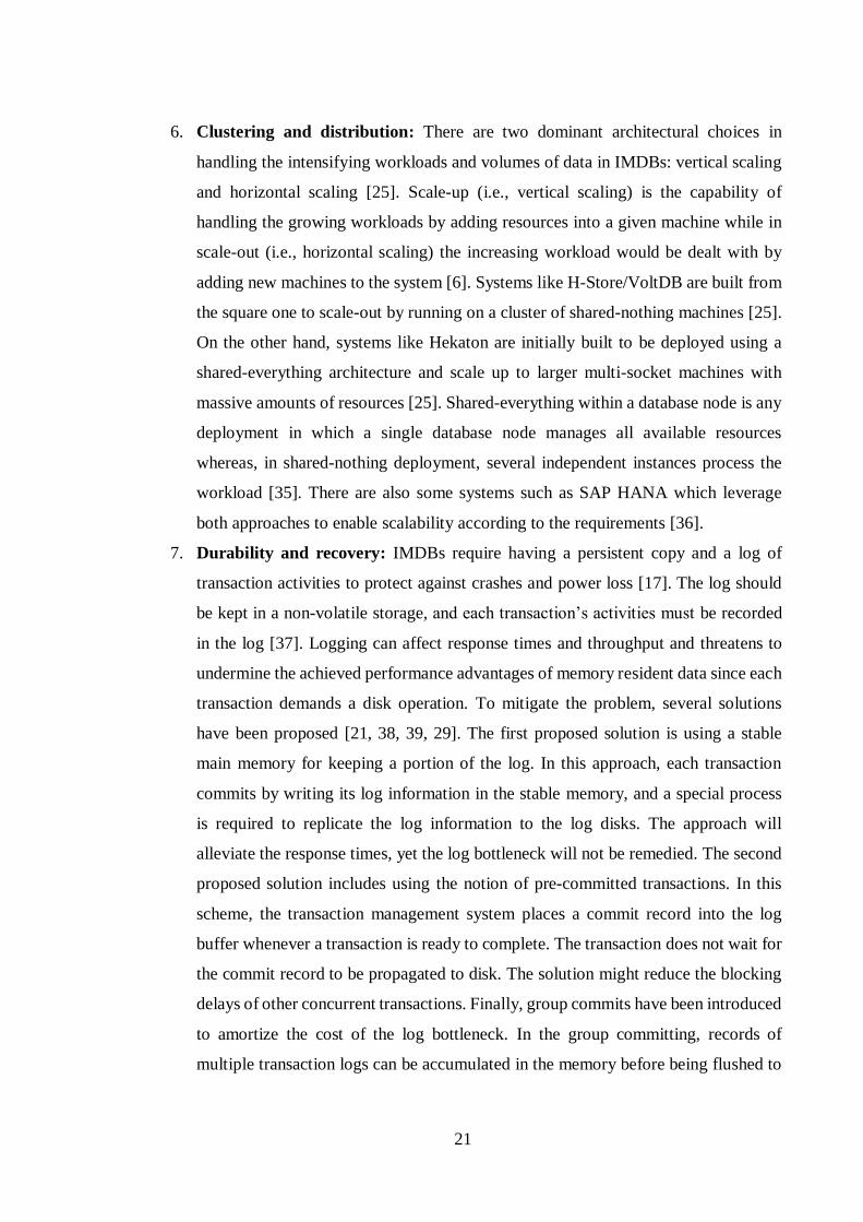
In the NUMA architecture, processors are grouped by their physical locations into NUMA
nodes (i.e., clusters), and each node has access to its local memory module. Even though the
nodes can access to memory associated with other nodes (called foreign memory or remote
memory), accessing the local memory is faster. Figure 5 demonstrates an overview of
memory architecture on Nehalem, a NUMA compatible processor produced by Intel. As
shown in the figure, quick path interconnect (QPI) coordinates access to remote memory. To
fully utilize the potentials of NUMA, applications should be implemented in a way to
primarily load data from the local associated memory and avoid remote memory access
latencies [7].
Figure 5 Memory architecture on Intel Nehalem [7]
2.1.4.2 Cache Efficiency
As described in Section 2.1.1, accessing the bottom levels in the memory hierarchy results
in high latencies. Thus, it is a reasonable approach to avoid accessing the lower levels as
much as possible. To this end, a crucial aspect in hiding the main memory latency is cache
efficiency [41]. Cache efficiency can be achieved through a fundamental principle: reference
locality. There are two kinds of the locality regarding memory access which are temporal
locality and spatial locality [7]. Temporal locality refers to the fact that whenever CPU
accesses an item in memory, it is likely to be reaccessed soon. Spatial locality refers to the
likelihood of accessing the adjacent memory cells while accessing a memory address.
Caches are organized in cache lines (e.g., the smallest unit of transfer between cache levels).
Whenever CPU requests to access a particular memory item, the item will be searched within
the cache lines. If the corresponding cache line is found, a cache hit will occur; otherwise, it
results in a cache miss. A cache efficient strategy will achieve a high hit/miss ratio.
Memory Page
Nehalem Quadcore
Core 0 Core 1 Core 2 Core 3
L3 Cache
L2
L1
TLB
Main Memory Main Memory
QPI
Nehalem Quadcore
Core 0 Core 1 Core 2 Core 3
L3 Cache
L2
L1
TLB
QPI
L1 Cacheline
L2 Cacheline
L3 Cacheline

24
2.1.4.3 Prefetching
A complementary solution to overcome the memory wall is using data prefetching. Data
prefetching is a technique that tries to guess which data will be accessed in advance and
loads the data before the data access. Modern processors support software and hardware
prefetching; Hardware prefetching utilizes multiple prefetching strategies to automatically
identify access patterns whereas software prefetching can be regarded as a hint to the
processor, implying the next address that will be accessed [7]. Data prefetching has been
widely used in data management systems. For example, Calvin, a transaction scheduling and
replication management layer for distributed storage systems, uses software prefetching in
transaction level [42]. After receiving a transaction request, Calvin performs a cursory
analysis of the transaction and sends a prefetch hint to storage back-ends contributing to the
transaction while it begins executing the transactions.
2.2 Hybrid Analytical/Transactional processing System
Applications handled by database systems can be classified into two main types: OLTP and
OLAP. The two next sections study the characteristics and requirements of the database
systems.
2.2.1 Online Transactional Processing Systems
According to [43], “A transaction processing application is a collection of transaction
programs designed to do the functions necessary to automate a given business activity.”
Transaction processing involves a wide variety of sectors of the economy like
manufacturing, banking, media, transportation. Transaction processing workloads fall into
two categories: batch processing and online processing. In batch transaction processing, a
series of transactions (called a batch) are processed without user interaction. Payroll and
billing systems are examples of the batch processing. Alternatively, in online transaction
processing, a transaction is executed corresponding to a request from an end-user device or
a front-end interface. Withdrawing money from an automated teller machine (ATM), placing
an order using an online catalog, and purchasing an online airline reservation system are
some examples of online transactions. In its early years, online transaction processing
25
systems were driven mostly by large enterprises. Nowadays, OLTP systems are omnipresent
even in small and mid-size businesses.
In the context of transaction processing, a transaction is a set of operations exhibiting a single
unit of work. A transaction is characterized by four properties: atomicity, consistency,
isolation, and durability (commonly referred as ACID). These properties [44] are discussed
below. ACID-compliancy is one of the essential requirements of OLTP systems.
▪ Atomicity: A transaction should be considered as a single unit of operations meaning
that either all the transactions’ operations should be completed or none of them. If a
transaction fails, all modifications applied by the transaction should be rolled back.
▪ Consistency: Running a transaction should maintain the consistency of the database
state. In other words, running a transaction transforms the state of a DBMS from a
consistent state to another consistent one. In particular, this includes that all integrity
constraints are met by transactions.
▪ Isolation: Changes made by a transaction must be isolated from the changes made by
other concurrent transactions accessing the same data. Put it differently, concurrent
transactions should affect the system in a manner that the transactions are executed
one at a time.
▪ Durability: Durability guarantees that after successful completion of a transaction,
the results will be permanent even in case of failures like power outages and system
crashes.
OLTP systems share some unique features which are listed as follows.
1. OLTP systems only rely on operational data and do not store historical data. In other
words, the systems only store current version of data.
2. OLTP schemas are usually normalized; the schemas are typically in 3NF or Boyce-
Code Normal Form (BCNF) to minimize the data entry volume and guarantee data
consistency. The high degree of normalization also stimulates inserts, updates, and
deletes while it might degrade data retrievals. [7]
3. OLTP queries are predominately simple and do not include complex joins,
aggregations, and groupings [10].

26
4. Number of users who frequently issue modifying statements is significant in OLTP
environments (OLTP environments are update-intensive) [11, 10]. As a result, the
systems deal with high levels of concurrency.
5. Typical OLTP queries only access one or a small number of sets, and only a few
tuples match their selection predicates [10].
6. OLTP systems mostly execute pre-determined queries [10]. In other words, ad-hoc
queries are not common in the systems.
7. OLTP systems demand swift response times. Psychological studies suggest that the
suitable maximum response time for a human is around three seconds [7]. To set a
tangible example, a person trying to dispense cache from an ATM expects his/her
transaction to be completed in few seconds. Considering that one or several
transactions might incorporate only some parts of a user interaction, each transaction
probably needs to be completed in milliseconds.
8. OLTP applications play a critical role in many enterprises, and there is no space for
compromising reliability, availability, or scalability [43].
In OLTP architectures, database management systems play an essential role since they are
the underlying entity managing the data shared by transaction processing applications. OLTP
systems are the predominant use case for relational DBMSs. The reasons for the dominance
are flexibility, performance, robustness, and simplicity in managing structured data. [15, 43]
2.2.2 Online Analytical Processing Systems
Computer-based analytics is not a new concept and have persisted even before the
emergence of relational database systems [6]. Management Information Systems (MISs) can
be regarded as the first generation of analytical systems introduced in 1965 with the
development of mainframe systems. At that time, the management information systems did
not support interactive data analysis. To support the interaction, decision support systems
(DSSs) are introduced in the 1970s. During the time, spreadsheets are the typical form of
DSSs widely used to derive information from raw data. However, the spreadsheets focus on
single users and are not able to provide a single view for multiple end-users. During the time,
continuous development of different transaction processing systems has instigated growing
heterogeneity in data sources. The term OLAP is coined in 1993 by Ted Codd referring to a

27
product which facilitates consolidation and of data from multiple sources in a
multidimensional space based on twelve rules [45]. In a multidimensional data model, there
is a set of measure attributes which represent the objects of analysis. Each of the attributes
depends on a set of dimensions which provides the analysis contexts. Additionally,
hierarchies can be defined within each dimension. Figure 6 demonstrates sale measurement
among city, product, and date dimensions. In the data model, the product includes a
hierarchy of industry and category.
Figure 6 An example of Multidimensional Data [46]
Like OLTP system, OLAP schemes share some distinct characteristics [10] which are listed
in the follows.
1. In OLAP systems ad-hoc queries are dominant.
2. OLAP queries predominately include complex joins, aggregations, and groupings.
3. Selection predicates in typical OLAP queries access a large number of sets.
4. OLAP queries are usually long-running.
5. OLAP queries are widely read-only.
6. Number of concurrent users running OLAP queries is small.
The substantial differences between transactional and analytical workloads are the reason
that many companies began to separate their OLTP databases from OLAP. In the 1990s,
Data Warehouses (DW, also called DWH) were developed as a foundation for analytical
workloads. DWHs mostly model information into multidimensional data cubes and apply
OLAP-oriented database management systems. To represent the multi-dimensional data
model, DWHs enact different schemas among which star, snowflake, and fact constellations

28
are the most widely used. Star schema includes a single fact table and a single table for each
dimension. The connection between the fact tables and the dimension tables is coordinated
using a foreign key. Figure 7 shows an example of a star schema. More recently, using
columnar databases has become of particular interest for analytical processing [9]. The
columnar databases are explained in sections 2.2.3 and 2.2.4.
Figure 7 A star schema [46]
OLAP operations can be classified into four groups [46] as detailed below.
• Rollup is performing aggregation on a data cube by reducing dimensions or climbing
up a concept hierarchy for a dimension.
• Drill-down is decreasing the amount of aggregation or expanding detail along one or
more dimension hierarchies.
• Slice and dice is selecting and projecting a dimension of a cube as a new sub-cube.
• Pivot is rotating the multidimensional view of data.
Data warehouses might be implemented on top of relational DBMS by mapping
multidimensional data into relations. The approach is called relational OLAP (ROLAP). It
is also possible to apply specific data structures to store the multidimensional data, which is
named multidimensional OLAP (MOLAP).
As mentioned, the data in a data warehouse is comprised of different OLTP systems and
external sources. Consequently, a process is required to consolidate the data from various
sources into DWHs. The method is named extract, transform, load (ETL) and consists of
three primary steps. During the extraction, the desired data is extracted from data sources.
The second stage includes converting the extracted data into a proper format consistent with
OLAP data structure. The process is completed by materializing the transformed data into
Fact table OrderNo SalespersonID CustomerNo DateKey
CityName ProdNo Quantity TotalPrice
Order OrderNo OrderDate
Customer CustomerNo CustomerName CustomerAddress City
Salesperson SalespersonID SalespesonName City Quota
ProdNo ProdName ProdDescr Category UnitPrice QOH
City CityName State
Date DateKey Date Month

29
target data storages. To maintain data freshness, the ETL process should be done periodically
(usually overnight).
2.2.3 Relational data layouts
In the relational data model, tables are used to represent the logical structure of data. Tables
(also called relations) include attributes and tuples. Hence, each relation consists of two
dimensions including rows (i.e., tuples) and columns (i.e., attributes). Table 1 demonstrates
a straightforward relation with five attributes and two tuples. To store a relation inside
memory, it is required to map the two-dimensional structure to a unidimensional memory
address space. There are two approaches to storing a relation in memory: row and columnar
layout [7].
ID FName LName City Country
1 Bahman Javadi Lappeenranta Finland
2 Ted Smith Walldorf Germany Table 1 Sample Relation
The row-based layout is the most classical way of representing relations in memory. The
layout stores relations in memory using a row-based (or record-based) structure. In other
words, the record-based layout will store tuples consecutively and sequentially in memory.
Considering the sample relation, the data would be stored as a sequence of tuples in memory
as follows, where each line represents a record stored in a memory region.
1 Bahman Javadi Lappeenranta Finland
2 Ted Smith Walldorf Germany
The second approach in storing the two-dimensional structures is storing relations based on
attributes. The approach is called columnar or column-oriented. In the columnar layout,
values of columns are store together. The columnar layout of the sample relation would be
as:
1 2
Bahman Ted
Javadi Smith
Finland Germany

30
Using the different memory layouts has a significant impact on memory access patterns as
shown in Figure 8 where A, B, and C represent three different columns of a table.
Considering set-based operations like aggregate calculations which only access a small
subset of columns, the columnar layout is more efficient since the values of columns will be
scanned sequentially in fewer CPU cycles. On the other hand, the row-wise layout
outperforms the column-wise for row-based operations which operate on a single or a set of
tuples (e.g., a projection using SELECT *). As a result, considering the workload should be
a significant factor in selecting the memory layout. Typically, the row-wise layout is mostly
used in OLTP databases since transactional queries are associated with row operations such
as accessing or modifying a few rows at a time. Conversely, columnar storages are more
suitable for OLAP queries that are characterized by large sequential scans traversing a few
attributes of a big set of tuples. It is also possible to use a combination of both row and
columnar layouts, a hybrid design. [9]
Figure 8 Memory access pattern for set-based and row-based operations on row and columnar data
layouts [7]
31
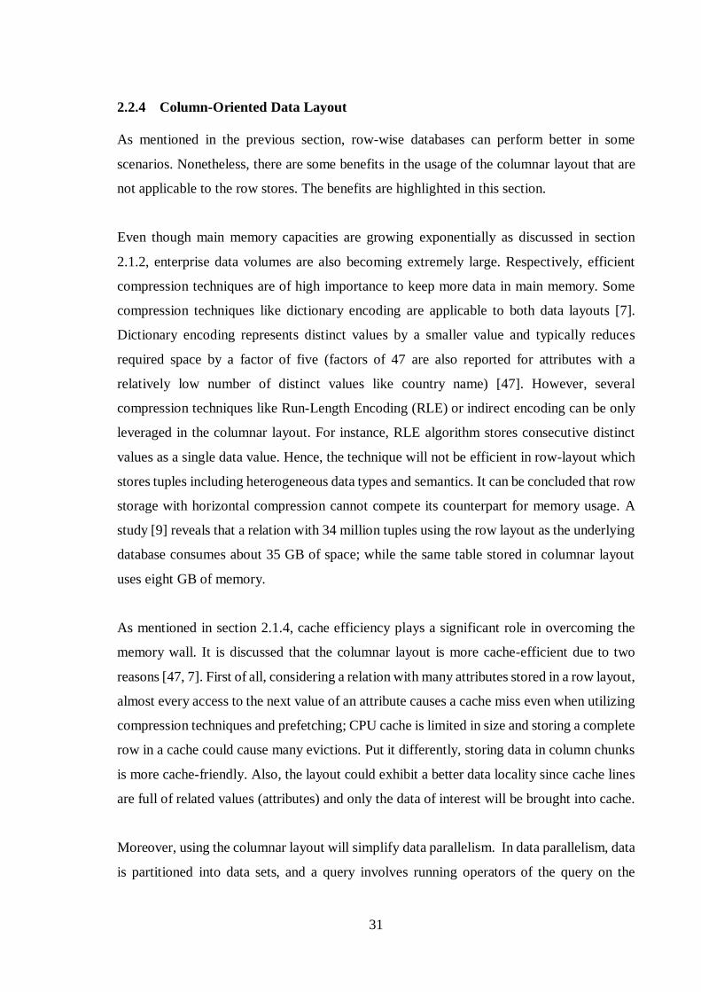
2.2.4 Column-Oriented Data Layout
As mentioned in the previous section, row-wise databases can perform better in some
scenarios. Nonetheless, there are some benefits in the usage of the columnar layout that are
not applicable to the row stores. The benefits are highlighted in this section.
Even though main memory capacities are growing exponentially as discussed in section
2.1.2, enterprise data volumes are also becoming extremely large. Respectively, efficient
compression techniques are of high importance to keep more data in main memory. Some
compression techniques like dictionary encoding are applicable to both data layouts [7].
Dictionary encoding represents distinct values by a smaller value and typically reduces
required space by a factor of five (factors of 47 are also reported for attributes with a
relatively low number of distinct values like country name) [47]. However, several
compression techniques like Run-Length Encoding (RLE) or indirect encoding can be only
leveraged in the columnar layout. For instance, RLE algorithm stores consecutive distinct
values as a single data value. Hence, the technique will not be efficient in row-layout which
stores tuples including heterogeneous data types and semantics. It can be concluded that row
storage with horizontal compression cannot compete its counterpart for memory usage. A
study [9] reveals that a relation with 34 million tuples using the row layout as the underlying
database consumes about 35 GB of space; while the same table stored in columnar layout
uses eight GB of memory.
As mentioned in section 2.1.4, cache efficiency plays a significant role in overcoming the
memory wall. It is discussed that the columnar layout is more cache-efficient due to two
reasons [47, 7]. First of all, considering a relation with many attributes stored in a row layout,
almost every access to the next value of an attribute causes a cache miss even when utilizing
compression techniques and prefetching; CPU cache is limited in size and storing a complete
row in a cache could cause many evictions. Put it differently, storing data in column chunks
is more cache-friendly. Also, the layout could exhibit a better data locality since cache lines
are full of related values (attributes) and only the data of interest will be brought into cache.
Moreover, using the columnar layout will simplify data parallelism. In data parallelism, data
is partitioned into data sets, and a query involves running operators of the query on the
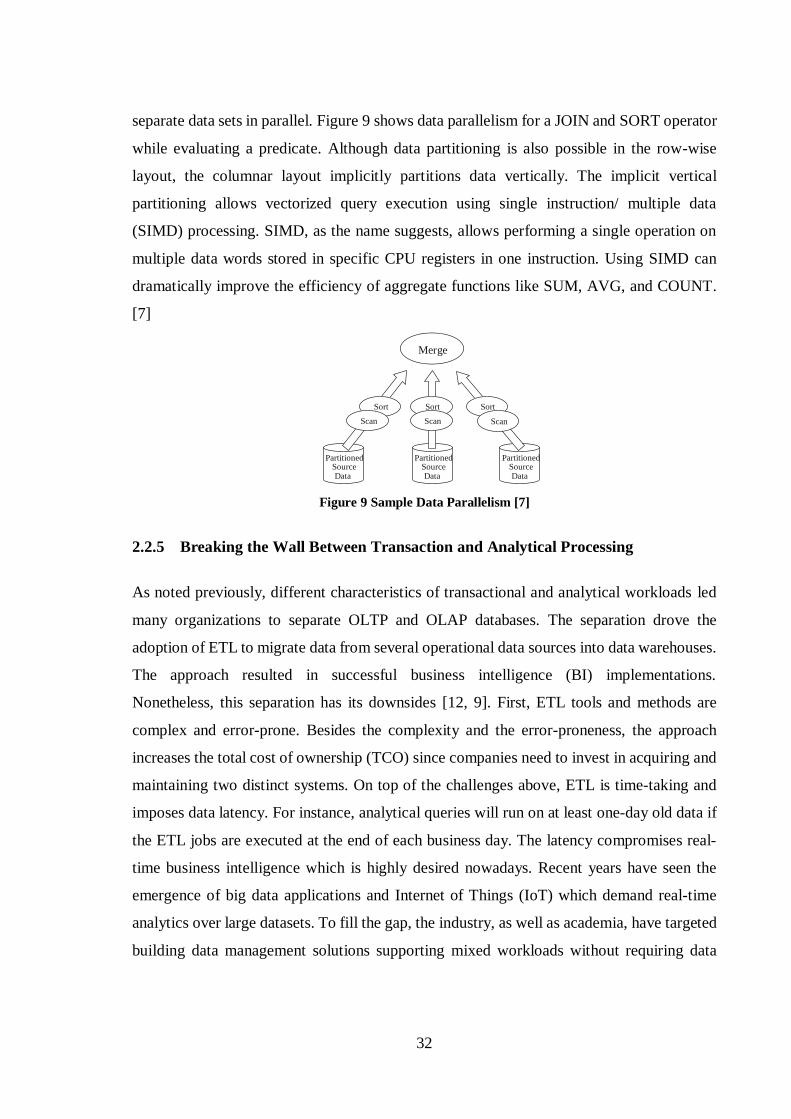
32
separate data sets in parallel. Figure 9 shows data parallelism for a JOIN and SORT operator
while evaluating a predicate. Although data partitioning is also possible in the row-wise
layout, the columnar layout implicitly partitions data vertically. The implicit vertical
partitioning allows vectorized query execution using single instruction/ multiple data
(SIMD) processing. SIMD, as the name suggests, allows performing a single operation on
multiple data words stored in specific CPU registers in one instruction. Using SIMD can
dramatically improve the efficiency of aggregate functions like SUM, AVG, and COUNT.
[7]
Figure 9 Sample Data Parallelism [7]
2.2.5 Breaking the Wall Between Transaction and Analytical Processing
As noted previously, different characteristics of transactional and analytical workloads led
many organizations to separate OLTP and OLAP databases. The separation drove the
adoption of ETL to migrate data from several operational data sources into data warehouses.
The approach resulted in successful business intelligence (BI) implementations.
Nonetheless, this separation has its downsides [12, 9]. First, ETL tools and methods are
complex and error-prone. Besides the complexity and the error-proneness, the approach
increases the total cost of ownership (TCO) since companies need to invest in acquiring and
maintaining two distinct systems. On top of the challenges above, ETL is time-taking and
imposes data latency. For instance, analytical queries will run on at least one-day old data if
the ETL jobs are executed at the end of each business day. The latency compromises real-
time business intelligence which is highly desired nowadays. Recent years have seen the
emergence of big data applications and Internet of Things (IoT) which demand real-time
analytics over large datasets. To fill the gap, the industry, as well as academia, have targeted
building data management solutions supporting mixed workloads without requiring data
Partitioned Source Data
Sort Scan
Merge
Partitioned Source Data
Sort Scan
Partitioned Source Data
Sort Scan

33
duplication. Hybrid transactional/analytical processing (HTAP) is a term coined by Gartner
to define such systems [48].
Several vendors currently offer HTAP systems such as HANA, VoltDB, and HyPer. Two
questions then arise: What are the primary enablers of the hybrid systems and how the
solutions mainly differ? It is discussed that in-memory database technologies and advances
in modern hardware (e.g., increasing main memory capacity, the advent of multi-core
processors, and levels of memory caches) can be considered as the principal drivers for rising
the systems [48, 12, 9, 13]. To support a single system for both OLTP and OLAP, HTAP
solutions today apply a variety of design practices like resource management and data layout.
For instance, HyPer can be configured as a row or column store and may utilize a virtual
memory (VM) snapshot to manage resource utilization for mixed workloads [13]. The VM
snapshot architecture generates consistent snapshots of the transactional data for OLAP
query sessions. The snapshots are created by forking a single OLTP process, and the
consistency of the snapshots are implicitly maintained by an OS/processor-controlled lazy
copy-on-update synchronization mechanism. By injecting OLAP-style queries into a
different queue, OLTP transactions will not wait for long-running analytical queries while
still access the current memory state of OLTP process. Likewise, SAP HANA employs
different design practices to handle mixed workloads. The system incorporates a row engine
which is suitable for extreme OLTP workloads as well as a column store optimized to
support OLAP and mixed workloads. The design of the column store enables both highly
efficient analytics and at the same time very decent OLTP performance, allowing both
workloads on a single copy of the data in main memory [12]. To support co-existence of
OLTP and OLAP queries, HANA utilizes a dynamic task scheduling mechanism for
servicing analytical queries expressed as a single or multiple tasks [49]. One worker thread
per hardware context continuously fetches tasks from queues and processes them. The
scheduler is responsible for balancing the number of worker threads according to the number
of hardware contexts. The scheduler also decides how OLTP and OLAP queries consume
resources according to an adjustable configuration.
As discussed in sections 2.2.1 and 2.2.2, OLTP workloads are characterized by update-
intensive and tuple-oriented operations while OLAP workloads are attributed to sequential

34
scans over a few attributes but many rows of the database. However, the typical DBMS
interaction pattern are also changing over the time: A study [50] turns out that read-oriented
set operations dominate actual workloads in modern enterprise applications. In other words,
OLTP and OLAP systems are not necessarily as different as typically explained. In the study,
the customers’ workloads of a business suite are analyzed as shown in Figure 10. The study
demonstrates that more than 80% of all OLTP and OLAP queries are read-access. Whereas
both systems deal with permanent modifications and inserts, the number of inserts and
modifications are a little higher on OLTP side. Also, lookup rate is only 10% higher in OLTP
systems compared to OLAP systems. The study concludes that a read-optimized data layout
will satisfy update operations for both workloads.
Figure 10 Comparison of OLTP and OLAP workloads based on distribution of query types extracted
from a customer database statistics [50]
2.3 OLTP WORKLOAD BENCHMARKS
Currently, a variety of benchmarks are available to measure the performance of database
management systems. These benchmarks not only provide a tool for vendors to improve
their products but also customers can achieve a comparison baseline using the benchmarks’
results. This section presents a brief study of two OLTP benchmarks:
• TPC-C (an open source benchmark provided by TPC)
• Sales and distribution (SD) benchmark (a proprietary benchmark provided by SAP)
35
2.3.1 TPC-C Benchmark
TPC is formed in 1988 as a non-profit corporation with the goal of standardizing objective,
and verifiable data-centric benchmarks [51]. From then on, the council has published about
16 benchmarks to measure the performance of different systems such as OLTP, OLAP, big
data, IoT, and so on. Among the standardized benchmarks, TPC-C is an online transaction
processing benchmark approved in 1992 and since then has been widely used in the industry
[50, 52].
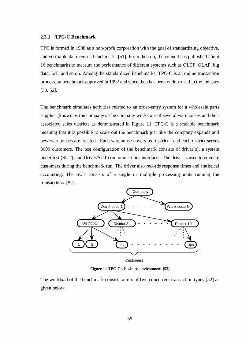
The benchmark simulates activities related to an order-entry system for a wholesale parts
supplier (known as the company). The company works out of several warehouses and their
associated sales districts as demonstrated in Figure 11. TPC-C is a scalable benchmark
meaning that it is possible to scale out the benchmark just like the company expands and
new warehouses are created. Each warehouse covers ten districts, and each district serves
3000 customers. The test configuration of the benchmark consists of driver(s), a system
under test (SUT), and Driver/SUT communications interfaces. The driver is used to emulate
customers during the benchmark run. The driver also records response times and statistical
accounting. The SUT consists of a single or multiple processing units running the
transactions. [52]
Figure 11 TPC-C's business environment [52]
The workload of the benchmark consists a mix of five concurrent transaction types [52] as
given below.
Customers
Company
Warehouse-1
District-10
Warehouse-N
District-1 District-2
k 3 1 2 30 k

36
• New-order: The transaction represents entering a complete order. It is a read-write
transaction having a high frequency of execution.
• Payment: This transaction represents updating a customer’s balance and reflecting
the payment on the company and the district sales statistics. Just like the new-order
transaction, it is a read-write transaction with a high frequency of execution.
• Delivery: The transaction incorporates delivering a batch up to 10 new orders. This
is a read-write transaction with a low execution frequency.
• Order-status: This is a read-only transaction with a low frequency of execution. The
order-status transaction queries the position of a customer’s last order.
• Stock-level: This is a read-only transaction with a low frequency of execution. It
queries the number of recently sold items below a specific threshold.
TPC-C requires that all ACID properties be maintained during the test. The benchmark
demands that at least 90% of all transactions except the stock-level to be completed within
5 seconds while the stock level transactions should be completed within 20 seconds. The
benchmark measures two metrics: One performance metric is in terms of the number of
completed new-order transactions per minute (called tpmC). The benchmark also requires
reporting a price-per-tpmC metric. The benchmark starts with a ramp-up phase in which
tpmC reaches a steady level. Then, the measurement interval starts and should continue for
at least 120 minutes. After the measurement interval, a ramp-down stage closes the
benchmark test-run. Figure 12 depicts a sample run graph of the benchmark. The x-axis
portrays the elapsed time from the beginning of the run as the y-axis sketches the Maximum
Qualified Throughput (MQTh) rating expressed in tpmC. TPC-C implementations must
scale both the number of customers and the size of the database proportionally to the
measured throughput. [52]

37
Figure 12 Sample TPC-C run graph [52]
The benchmark’s database comprises nine individual tables as sketched in Figure 13.
Numbers inside the entity blocks exhibit the cardinality of the tables whereas those numbers
starting with W denotes a scaling factor of the number of warehouses. The numbers next to
relationship arrows show the average cardinality of the relationships. The plus symbol after
the relationships’ cardinality demonstrates that the number is subject to a small variation in
the initial database population over the measurement interval. [52]
Figure 13 TPC-C ER diagram of tables and relationships among them [52]
2.3.2 SD Benchmark
Similarly to TPC, SAP offers a variety of benchmarks for different business scenarios under
the umbrella of SAP Standard Application Benchmark suite. The business scenarios include
Sales and Distribution (SD), Assemble-to-Order (ATO), production planning (PP), and
many more. The suite is developed and published in 1993 to facilitate necessary sizing
recommendations of SAP systems and for platform comparisons. SAP Application
Ramp - up Steady State Ramp - down
Elapsed Time ( sec. ) 0
MQTh
Measurement Interval Start
Measurement Interval End
Warehouse District
History
Customer New-Order
Order Order-Line Item
Stock
W W*10
3 k
1+
W*30k
W*30k+ 5-15
0-1
1+ W*30k+
W*9k+
W*300k+
3+
100 k
W
W*100k
100 k
10
38
Benchmark Performance Standard (SAPS) is the metric of measurement in the suite and
expresses the performance of a system configuration in the SAP environment. SAPS is
derived from the Sales and Distribution (SD) benchmark in a manner that 2000 fully
processed order line items per hour are equivalent to 100 SAPS. Fully processed here means
that the entire process of an order line item including creating the order, creating the delivery
note for the order, viewing the order, making changes to the delivery, posting an item issue,
listing orders, and generating an invoice has to be completed. In technical terms, this is
equivalent to 6000 dialog steps plus 2000 postings per hour in the SD benchmarks, or 2400
SAP transactions. A dialog step imitates a screen change corresponding to a user request.
[53]
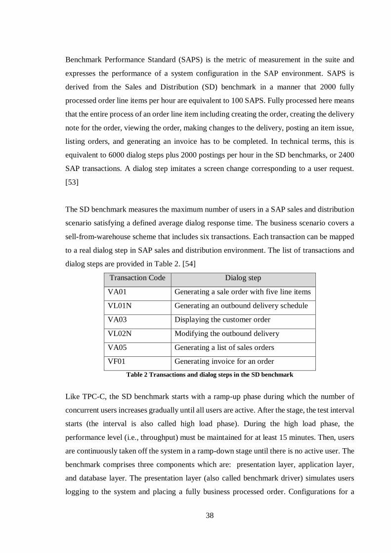
The SD benchmark measures the maximum number of users in a SAP sales and distribution
scenario satisfying a defined average dialog response time. The business scenario covers a
sell-from-warehouse scheme that includes six transactions. Each transaction can be mapped
to a real dialog step in SAP sales and distribution environment. The list of transactions and
dialog steps are provided in Table 2. [54]
Transaction Code Dialog step
VA01 Generating a sale order with five line items
VL01N Generating an outbound delivery schedule
VA03 Displaying the customer order
VL02N Modifying the outbound delivery
VA05 Generating a list of sales orders
VF01 Generating invoice for an order
Table 2 Transactions and dialog steps in the SD benchmark
Like TPC-C, the SD benchmark starts with a ramp-up phase during which the number of
concurrent users increases gradually until all users are active. After the stage, the test interval
starts (the interval is also called high load phase). During the high load phase, the
performance level (i.e., throughput) must be maintained for at least 15 minutes. Then, users
are continuously taken off the system in a ramp-down stage until there is no active user. The
benchmark comprises three components which are: presentation layer, application layer,
and database layer. The presentation layer (also called benchmark driver) simulates users
logging to the system and placing a fully business processed order. Configurations for a
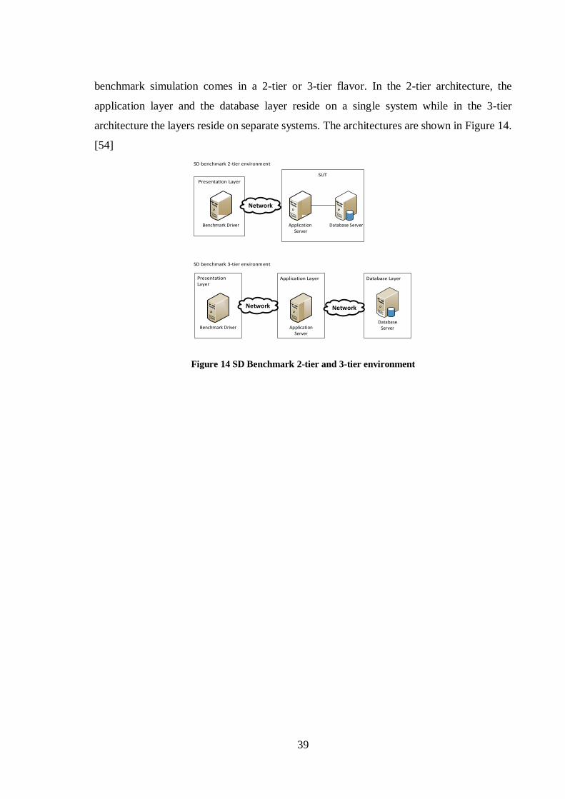
39
benchmark simulation comes in a 2-tier or 3-tier flavor. In the 2-tier architecture, the
application layer and the database layer reside on a single system while in the 3-tier
architecture the layers reside on separate systems. The architectures are shown in Figure 14.
[54]
Benchmark Driver
Network
Application Server
Database Server
Benchmark Driver
Network
ApplicationServer
Network
DatabaseServer
Figure 14 SD Benchmark 2-tier and 3-tier environment

40
2.4 SAP HANA
SAP HANA is an in-memory database offered by SAP. Initially, the system was built from
the ground up to support only analytical workloads [12]. However, it unfolded over the
course of time from a pure analytical appliance to a system capable of handling mixed
workloads. The evolutionary process of this system is not a one-time journey: In fact, the
system evolved within three steps. The following subsections study the steps and the major
developments in each stage.
2.4.1 HANA for Analytical Workloads
The initial architecture of the scheme was based on providing a sound basis for analytical
processing. SAP employed three design principles [12] in developing HANA: (1)
performing extensive parallelization, (2) embracing a scan-friendly data layout, and (3)
supporting advanced analytical engine capabilities.
Massive parallelization at all levels is one of the core design principles of SAP HANA
motivated by recent trends in developing many-core CPUs. HANA supports parallel query
processing at different levels. Inter-query parallelism is achieved by maintaining multiple
concurrent user sessions. Intra-query parallelism is gained by running different operations
within a single query in parallel. HANA also supports intra-operator parallelism by
executing individual operators in multiple threads.
Moreover, HANA relies on a columnar data layout to provide a scan-friendly foundation for
analytical queries. HANA columnar layout is accompanied by dictionary compression and
hardware prefetchers to minimize memory consumption while hiding memory access
latencies. Besides, SAP HANA presents a rich collection of analytical engines including
geospatial, graph, text, and planning engines.
2.4.2 HANA for Transactional Workloads
Over the course of time, SAP decided to broaden the scope of HANA from a pure analytical
processing toward a system also supporting OLTP workload. Although the system comes
with a row-store suitable for transactional workloads, the evolution of HANA toward

41
transactional processing was mostly based on optimizing the column store. SAP enacted
several tunings to maintain OLTP workloads, as follows.
• Query compilation in OLTP queries can dominate query run-times; To avoid re-
compiling frequently executed statements, the system inserts the compiled query
plans into a cache (i.e., query plan cache) [12]. When a query needs to be executed
later, HANA checks for a corresponding execution plan in the cache. The system
reuses the cached plan it finds, saving the overhead of recompilation.
• As previously mentioned, the column store in SAP HANA is encoded using a
dictionary-based compression. Nevertheless, using the compression has an overhead
of re-encoding for update operations. To minimize the overhead of frequent updates,
each column in the column store is composed of two tables: a read-optimized main
table, and a write-optimized delta table [55]. The main table uses a sorted dictionary
to speed up scans while the delta tables use an unsorted dictionary to enhance update
operations. The delta table includes recently added, deleted, and updated data. In
other words, update operations only affect this table. During the read operations, both
tables will be queried. The delta tables will be periodically merged into the main
tables. Figure 15 portrays the use of the main and delta tables in HANA columnar
storage.
Figure 15 (a) The core data structures of the main and the delta parts of a column. (b) The
delta merge operation. [55]
• In OLTP scenarios, it is often found columns that store only a single or empty value.
In case of finding a single default value, HANA bypasses storing the value in a
columnar representation and stores it inside the column header. This optimization
could amplify throughput and improve CPU consumption. [12]
• SAP HANA relies on snapshot isolation concurrency control in transaction
management. The transaction manager in its initial version was based on a visibility
tracking mechanism via an explicit bit-vector per transaction on table-level.
42
However, the tracking mechanism turned out to be expensive and memory-
consuming for transactional workloads. To handle this shortfall, HANA applied a
new row-based visibility tracking mechanism depending on time-stamps associated
with each row. The timestamp indicates when the row is created or deleted. Further,
the timestamps can be periodically replaced by a bit indicating the rows’ visibility to
reduce memory consumption overhead. [12]
• Efficient synchronization of in-memory data structures has a critical effect on
scalability and performance of transactional database systems. To maintain both the
performance and the scalability, HANA carefully optimizes table latching and
applies advanced synchronization primitives. For instance, Intel Transaction
Synchronization Extensions (TSX) is used in the system to decrease lock
contentions. [12]
• SAP HANA exploits application-server/DBMS co-design for efficient data transfer.
Advanced Business Application Programming (ABAP) is a platform for developing
business applications on top of SAP HANA. The platform comprises ABAP
programming language and its runtime including an application server. HANA
natively optimizes for the platform. For instance, Fast Data Access (FDA) is a feature
which enables efficient data transfer by directly reading and writing into special data
structures shared between the database system and ABAP application server. [12]
2.4.3 HANA for Mixed Workloads
In the final step of the journey, SAP took a disruptive approach toward extending HANA to
an HTAP system on top of OLTP-style database schema [12]. SAP employed three design
practices to achieve this goal:
• Resource management is a major challenge in handling mixed workloads since
analytical queries are resource-intensive and might result in delayed transactional
queries. Within SAP HANA, a scheduler is responsible for running queries and
monitoring resource utilization as described in section 2.2.5.
• In HANA, full columns are loaded into main memory during the first access;
subsequently, the loaded columns might be unloaded in case of memory pressure
[12]. Keeping both historical and operational data inside main memory might be
expensive as well as inefficient since the rarely accessed, historical data might cause
43
eviction of frequently accessed columns. SAP HANA make use of a data aging
process to identify certain data as cold (A.K.A aged data) or warm. There are two
techniques to store the cold data. The aged columns can be declared as page-loadable
inside the system [56]. The page-loadable columns are partially loaded into main
memory upon a request. It is also possible to store the aged data on disk to reduce
the memory footprint in HANA. Storing the cold data on disk using a separate storage
engine is called dynamic-tiering [57].
• Executing analytical queries on normalized database schemas requires data-models
suitable for reporting purposes. SAP HANA employs a layered architecture of
database views to facilitate analytics queries; the hierarchy of views are called Core
Data Services (CDS) views [58]. These views provide a rich semantic data model
consisting of layered views on top of normalized relational schemas.
44
2.4.4 SAP HANA SQLSCRIPT
As of today, there are two approaches to implement data-intensive business logic. A classical
approach is executing application logic in an application layer and leaving the database only
to perform limited functionality using SQL. This approach has two main drawbacks [59].
First, running business logic in another layer than database requires data transfer within the
two layers; the data transfer could be expensive regarding processor and transfer time.
Secondly, in this approach developers mostly follow a single-tuple-at-a-time semantic that
decreases the chance for leveraging query optimization and parallelization. In the second
model, the application logic will be shipped into the database layer. Relational databases
traditionally offer imperative language extensions using a dialect of SQL such as Procedural
Language/Structured Query Language(PL/SQL) or Transact-SQL(T-SQL) [60]. SAP
HANA exposes an interface for pushing the application logic to the database which is called
SQLScript.
SQLScript addresses several limitations with pure SQL statements. First, decomposing
complex SQL queries is only possible using views. The decomposition using views requires
that all intermediate results be visible and explicitly typed. The SQL views also cannot be
parameterized. SQLScript facilitates the decomposition by assignments and parametrization.
Secondly, SQL statements do not have features for expressing business logic (e.g., currency
conversion). SQLScripts provides three extensions to the SQL dialect of HANA: an
imperative (procedural), a declarative (functional), and a data extension. Furthermore, an
SQL query can only return single result at a time. Hence, computation of related result sets
should be split into usually unrelated, separate queries. SQLScript offers multiple input and
output parameter to overcome this deficit. [60]
2.4.4.1 SQLScript Data Extension
The data extension in SQLScript is based on the SQL-92 type system. The built-in supported
scalar data types comprise of the ones shown in Table 3. The extension also allows defining
table types for tabular values. The syntax for defining table variables is similar to the SQL
syntax for defining a new table. For instance, “CREATE TYPE tt_year AS TABLE (year
VARCHAR(4), price DECIMAL, cnt INTEGER)“ defines a table type named tt_year
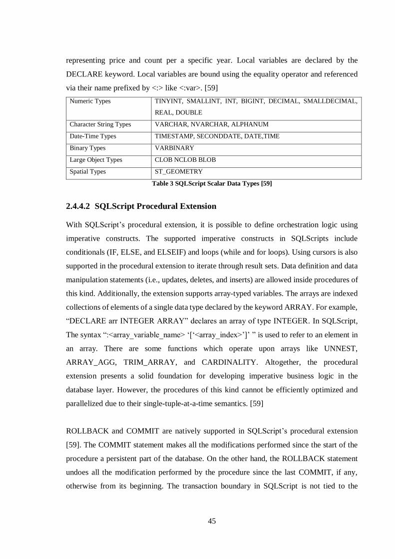
45
representing price and count per a specific year. Local variables are declared by the
DECLARE keyword. Local variables are bound using the equality operator and referenced
via their name prefixed by <:> like <:var>. [59]
Numeric Types TINYINT, SMALLINT, INT, BIGINT, DECIMAL, SMALLDECIMAL,
REAL, DOUBLE
Character String Types VARCHAR, NVARCHAR, ALPHANUM
Date-Time Types TIMESTAMP, SECONDDATE, DATE,TIME
Binary Types VARBINARY
Large Object Types CLOB NCLOB BLOB
Spatial Types ST_GEOMETRY
Table 3 SQLScript Scalar Data Types [59]
2.4.4.2 SQLScript Procedural Extension
With SQLScript’s procedural extension, it is possible to define orchestration logic using
imperative constructs. The supported imperative constructs in SQLScripts include
conditionals (IF, ELSE, and ELSEIF) and loops (while and for loops). Using cursors is also
supported in the procedural extension to iterate through result sets. Data definition and data
manipulation statements (i.e., updates, deletes, and inserts) are allowed inside procedures of
this kind. Additionally, the extension supports array-typed variables. The arrays are indexed
collections of elements of a single data type declared by the keyword ARRAY. For example,
“DECLARE arr INTEGER ARRAY” declares an array of type INTEGER. In SQLScript,
The syntax “:<array_variable_name> ‘[‘<array_index>’]’ ” is used to refer to an element in
an array. There are some functions which operate upon arrays like UNNEST,
ARRAY_AGG, TRIM_ARRAY, and CARDINALITY. Altogether, the procedural
extension presents a solid foundation for developing imperative business logic in the
database layer. However, the procedures of this kind cannot be efficiently optimized and
parallelized due to their single-tuple-at-a-time semantics. [59]
ROLLBACK and COMMIT are natively supported in SQLScript’s procedural extension
[59]. The COMMIT statement makes all the modifications performed since the start of the
procedure a persistent part of the database. On the other hand, the ROLLBACK statement
undoes all the modification performed by the procedure since the last COMMIT, if any,
otherwise from its beginning. The transaction boundary in SQLScript is not tied to the
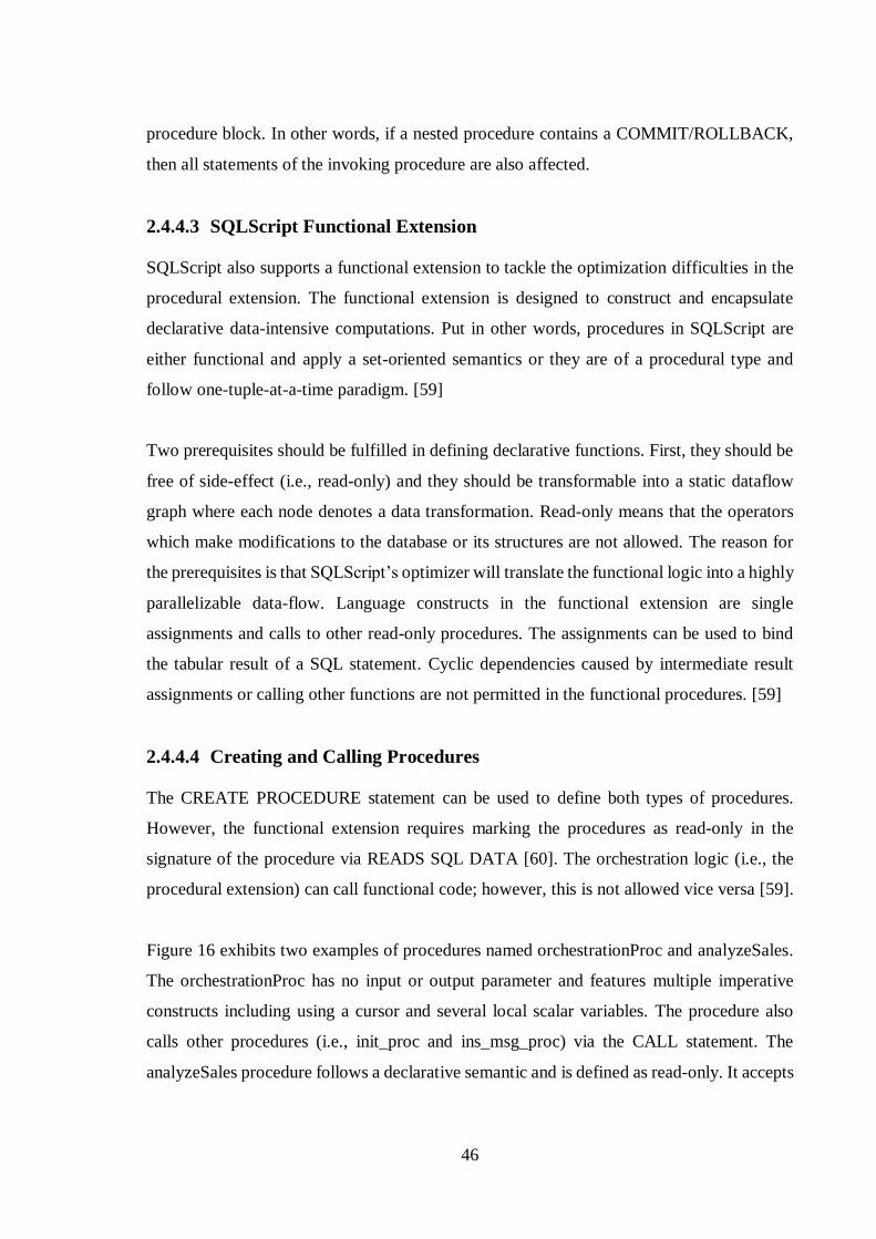
46
procedure block. In other words, if a nested procedure contains a COMMIT/ROLLBACK,
then all statements of the invoking procedure are also affected.
2.4.4.3 SQLScript Functional Extension
SQLScript also supports a functional extension to tackle the optimization difficulties in the
procedural extension. The functional extension is designed to construct and encapsulate
declarative data-intensive computations. Put in other words, procedures in SQLScript are
either functional and apply a set-oriented semantics or they are of a procedural type and
follow one-tuple-at-a-time paradigm. [59]
Two prerequisites should be fulfilled in defining declarative functions. First, they should be
free of side-effect (i.e., read-only) and they should be transformable into a static dataflow
graph where each node denotes a data transformation. Read-only means that the operators
which make modifications to the database or its structures are not allowed. The reason for
the prerequisites is that SQLScript’s optimizer will translate the functional logic into a highly
parallelizable data-flow. Language constructs in the functional extension are single
assignments and calls to other read-only procedures. The assignments can be used to bind
the tabular result of a SQL statement. Cyclic dependencies caused by intermediate result
assignments or calling other functions are not permitted in the functional procedures. [59]
2.4.4.4 Creating and Calling Procedures
The CREATE PROCEDURE statement can be used to define both types of procedures.
However, the functional extension requires marking the procedures as read-only in the
signature of the procedure via READS SQL DATA [60]. The orchestration logic (i.e., the
procedural extension) can call functional code; however, this is not allowed vice versa [59].
Figure 16 exhibits two examples of procedures named orchestrationProc and analyzeSales.
The orchestrationProc has no input or output parameter and features multiple imperative
constructs including using a cursor and several local scalar variables. The procedure also
calls other procedures (i.e., init_proc and ins_msg_proc) via the CALL statement. The
analyzeSales procedure follows a declarative semantic and is defined as read-only. It accepts
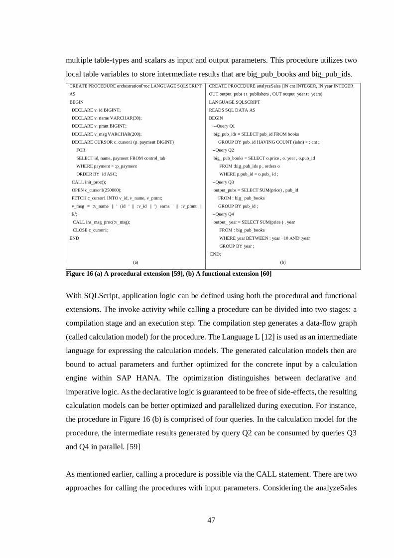
47
multiple table-types and scalars as input and output parameters. This procedure utilizes two
local table variables to store intermediate results that are big_pub_books and big_pub_ids.
CREATE PROCEDURE orchestrationProc LANGUAGE SQLSCRIPT
AS
BEGIN
DECLARE v_id BIGINT;
DECLARE v_name VARCHAR(30);
DECLARE v_pmnt BIGINT;
DECLARE v_msg VARCHAR(200);
DECLARE CURSOR c_cursor1 (p_payment BIGINT)
FOR
SELECT id, name, payment FROM control_tab
WHERE payment > :p_payment
ORDER BY id ASC;
CALL init_proc();
OPEN c_cursor1(250000);
FETCH c_cursor1 INTO v_id, v_name, v_pmnt;
v_msg = :v_name || ' (id ' || :v_id || ') earns ' || :v_pmnt ||
' $.';
CALL ins_msg_proc(:v_msg);
CLOSE c_cursor1;
END
CREATE PROCEDURE analyzeSales (IN cnt INTEGER, IN year INTEGER,
OUT output_pubs t t_publishers , OUT output_year tt_years)
LANGUAGE SQLSCRIPT
READS SQL DATA AS
BEGIN
--Query Q1
big_pub_ids = SELECT pub_id FROM books
GROUP BY pub_id HAVING COUNT (isbn) > : cnt ;
--Query Q2
big_ pub_books = SELECT o.price , o. year , o.pub_id
FROM :big_pub_ids p , orders o
WHERE p.pub_id = o.pub_ id ;
--Query Q3
output_pubs = SELECT SUM(price) , pub_id
FROM : big_ pub_books
GROUP BY pub_id ;
--Query Q4
output_ year = SELECT SUM(price ) , year
FROM : big_pub_books
WHERE year BETWEEN : year −10 AND :year
GROUP BY year ;
END;
(a) (b)
Figure 16 (a) A procedural extension [59], (b) A functional extension [60]
With SQLScript, application logic can be defined using both the procedural and functional
extensions. The invoke activity while calling a procedure can be divided into two stages: a
compilation stage and an execution step. The compilation step generates a data-flow graph
(called calculation model) for the procedure. The Language L [12] is used as an intermediate
language for expressing the calculation models. The generated calculation models then are
bound to actual parameters and further optimized for the concrete input by a calculation
engine within SAP HANA. The optimization distinguishes between declarative and
imperative logic. As the declarative logic is guaranteed to be free of side-effects, the resulting
calculation models can be better optimized and parallelized during execution. For instance,
the procedure in Figure 16 (b) is comprised of four queries. In the calculation model for the
procedure, the intermediate results generated by query Q2 can be consumed by queries Q3
and Q4 in parallel. [59]
As mentioned earlier, calling a procedure is possible via the CALL statement. There are two
approaches for calling the procedures with input parameters. Considering the analyzeSales
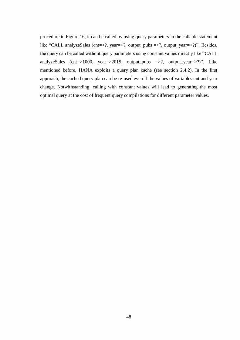
48
procedure in Figure 16, it can be called by using query parameters in the callable statement
like “CALL analyzeSales (cnt=>?, year=>?, output_pubs =>?, output_year=>?)”. Besides,
the query can be called without query parameters using constant values directly like “CALL
analyzeSales (cnt=>1000, year=>2015, output_pubs =>?, output_year=>?)”. Like
mentioned before, HANA exploits a query plan cache (see section 2.4.2). In the first
approach, the cached query plan can be re-used even if the values of variables cnt and year
change. Notwithstanding, calling with constant values will lead to generating the most
optimal query at the cost of frequent query compilations for different parameter values.
49
2.5 TPC-E Benchmark
TPC-E is an OLTP benchmark approved by TPC in 2007. This benchmark models the
activities of a stock brokerage firm as illustrated in Figure 17 (b). The activities include (1)
managing customer accounts, (2) executing customer trade orders, and (3) organizing
interactions between customers and financial markets. The benchmark focuses on measuring
the performance of the central database running transactions associated to the firm’s
customer accounts. Although the benchmark exhibits the activities of a brokerage firm, its
design is based on simulating the activities found in a complex transactional environment.
[61]
(a) (b)
Figure 17 (a) TPC-E application components (b) TPC-E business model transaction flow [61]
As highlighted in section 2.3.1, TPC-C is approved in 1992, and it follows an old-fashioned
OLTP environment. Consequently, TPC-E is designed to incorporate more current
requirements like realistic data skews and referential integrity requirements. Table 4
compares TPC-E with its predecessor, TPC-C. Firstly, TPC-E defines over three times as
the number of tables as TPC-C. Secondly, TPC-E has twice as number of columns as its
ancestor. Thirdly, TPC-E is more read-intensive than TPC-C, and the number of transaction
types is twice as defined in TPC-C. Furthermore, TPC-E exhibits realistic data skews by
populating the database with pseudo-real data. TPC-E data generator is based on U.S. census
data and actual listings on New York Stock Exchange (NYSE). Finally, TPC-C lacks
multiple features that are found in real-world transactional systems like check constraints
and referential integrity while TPC-E incorporates such requirements. In summary, TPC-E
is a more accurate OLTP benchmark compared to TPC-C, yet its implementation and test
setup is more sophisticated. [62]
Customers Brokers Market
READ-WRITE
•Market-Feed
•Trade-Order
•Trade-Result
•Trade-Update
•Security-Detail
•Trade-Lookup
•Trade-Status
READ-ONLY
•Broker-Volume
•Customer-Position
•Market-Watch
Invoke the following transactions …
… against the following data
Customer Data Brokerage Data Market Data
Customers Brokers Market
READ-WRITE
•Market-Feed
•Trade-Order
•Trade-Result
•Trade-Update
•Security-Detail
•Trade-Lookup
•Trade-Status
READ-ONLY
•Broker-Volume
•Customer-Position
•Market-Watch
READ-WRITE
•Market-Feed
•Trade-Order
•Trade-Result
•Trade-Update
•Security-Detail
•Trade-Lookup
•Trade-Status
READ-ONLY
•Broker-Volume
•Customer-Position
•Market-Watch
Invoke the following transactions …
… against the following data
Customer Data Brokerage Data Market Data
Customer
Brokerage
Market
Customer Initiated Txn
Market Triggered Txn
CustomerCustomer
BrokerageBrokerage
MarketMarket
Customer Initiated Txn
Market Triggered Txn
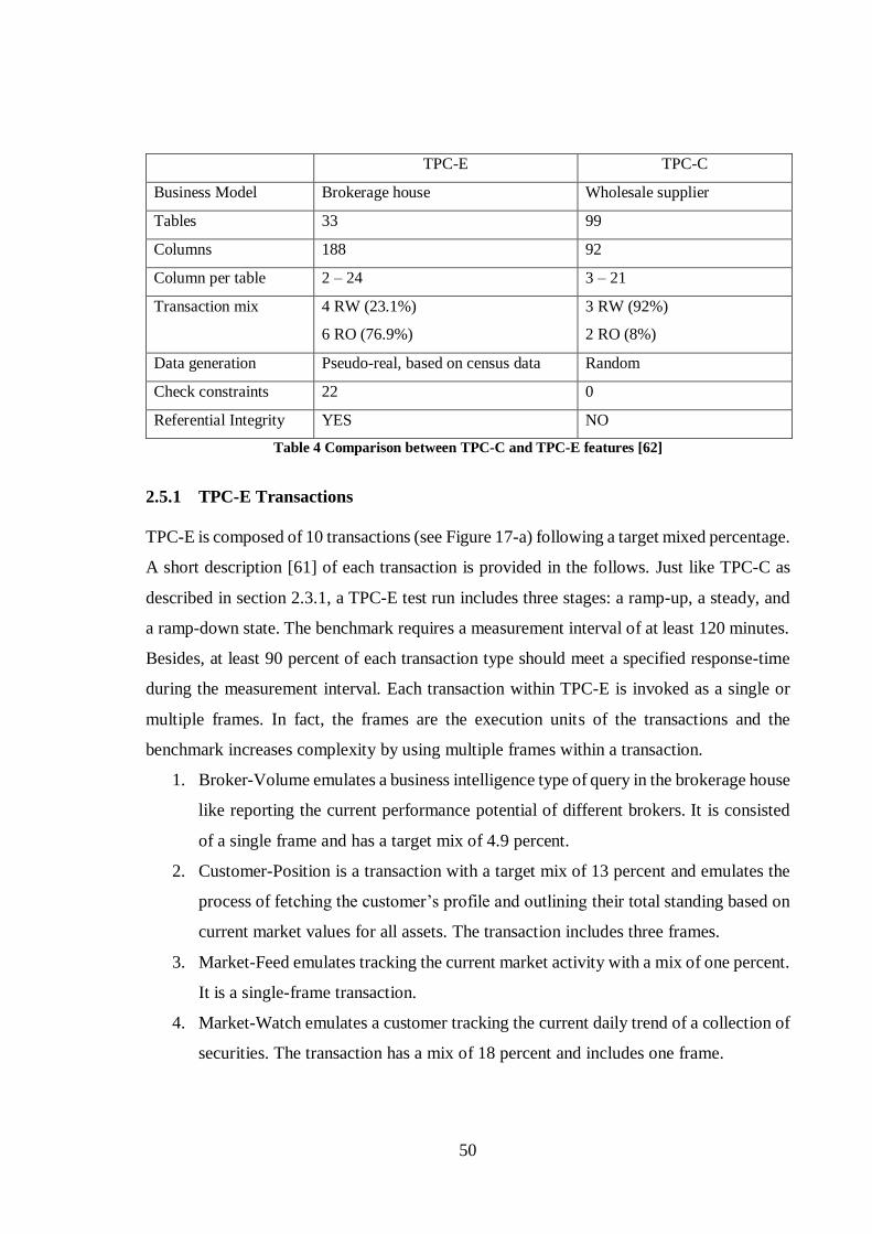
50
TPC-E TPC-C
Business Model Brokerage house Wholesale supplier
Tables 33 99
Columns 188 92
Column per table 2 – 24 3 – 21
Transaction mix 4 RW (23.1%)
6 RO (76.9%)
3 RW (92%)
2 RO (8%)
Data generation Pseudo-real, based on census data Random
Check constraints 22 0
Referential Integrity YES NO
Table 4 Comparison between TPC-C and TPC-E features [62]
2.5.1 TPC-E Transactions
TPC-E is composed of 10 transactions (see Figure 17-a) following a target mixed percentage.
A short description [61] of each transaction is provided in the follows. Just like TPC-C as
described in section 2.3.1, a TPC-E test run includes three stages: a ramp-up, a steady, and
a ramp-down state. The benchmark requires a measurement interval of at least 120 minutes.
Besides, at least 90 percent of each transaction type should meet a specified response-time
during the measurement interval. Each transaction within TPC-E is invoked as a single or
multiple frames. In fact, the frames are the execution units of the transactions and the
benchmark increases complexity by using multiple frames within a transaction.
1. Broker-Volume emulates a business intelligence type of query in the brokerage house
like reporting the current performance potential of different brokers. It is consisted
of a single frame and has a target mix of 4.9 percent.
2. Customer-Position is a transaction with a target mix of 13 percent and emulates the
process of fetching the customer’s profile and outlining their total standing based on
current market values for all assets. The transaction includes three frames.
3. Market-Feed emulates tracking the current market activity with a mix of one percent.
It is a single-frame transaction.
4. Market-Watch emulates a customer tracking the current daily trend of a collection of
securities. The transaction has a mix of 18 percent and includes one frame.

51
5. Security-Detail represents a customer investigating a security before deciding about
executing a trade. This single-frame transaction comprises 14 percent of total
transactions.
6. Trade-Lookup exhibits information retrieval by a customer or a broker to analyze a
set of trades. This transaction comprises of four frames and incorporates eight percent
of the whole transactions.
7. Trade-Order is designed to imitate a customer, broker, or authorized third-party that
sells or buys a security. The trading person can trade at the current market price or
place a limit order. Transactions of this type take in 10.1 percent of the total mix.
Also, it encompasses six frames.
8. Trade-Result emulates the process of finalizing a stock market trade within six
frames. The transaction involves 10 percent of the total mix.
9. Trade-Status is a single-frame transaction with 19 percent mix percentage that
portrays a customer checking a summary of the recent trading actions for one of their
accounts.
10. Trade-Update is a transaction with three frames which emulates the process of
updating a set of trades. In total, 2 percent of total transactions are of this type.
As mentioned earlier, TPC-E imposes constraints on response times during the measurement
interval. According to the benchmark’s specification, 90 percent of the Trade-Status
transactions must be completed within 1 second. Likewise, the Market-Feed, Trade-Order,
and Trade-Result transactions must have a response time below two seconds. All other
transactions that are part of the maintained transaction mix have a required response time
within the bounds of three seconds. Besides the mentioned transactions, there are two other
transactions which are not a part of the mixed transactions including Data-Maintenance and
Trade-Cleanup. The Data-Maintenance is a time-triggered transaction that must be invoked
once each minute and completed in 55 seconds or less. It emulates periodic modifications to
the database and is similar to updating data that seldom changes. The Trade-Cleanup
transaction runs once at the start of test-run and cancels pending or submitted trades from
the database. [61]

52
2.5.2 TPC-E Required Isolation Levels
The benchmark demands to enforce full ACID properties during the test run. TPC-E defines
four concurrency anomalies: Dirty-read, dirty-write, non-repeatable read, and phantom read.
The dirty-write phenomenon happens while a transaction can modify an intermediate,
uncommitted data element from another transaction and commit the changes. In the same
way, the dirty-read occurs when a transaction can access any intermediate, uncommitted data
element from another transaction. The non-repeatable read occurs, when a data element is
retrieved twice during a transaction, and the values differ between reads. Finally, the
phantom read happens, when two identical read queries in a transaction obtain different sets
of data elements. [61]
According to [61], three types of isolations must be retained during a test run. The dirty-
read and dirty-write anomalies must not occur in the Broker-Volume, Customer-Position,
Data-Maintenance, Market-Watch, Security-Detail, Trade-Lookup, and Trade-Status
transactions. The Market-Feed and Trade-Order transactions should also be isolated from
the non-repeatable reads. Besides, the Trade-Result transactions should keep the highest
level of isolation and be prevented from the phantom reads.
2.5.3 Scaling the Benchmark
TPC-E has three primary metrics including a performance metric, a price metric, and an
availability date. The price metric is TPC-E three years pricing divided by the reported
throughput. The availability date is the date that all products required to achieve the reported
throughput will be available. The performance metric is of particular interest to the thesis;
more explicitly, the other metrics are ignored. The performance metric is expressed in
transactions-per-second-E (tpsE). The tpsE is calculated by the number of Trade-Result
transactions that complete in a one-minute interval divided by 60. Measuring the throughput
should be done during a measurement interval with at least 120 minutes. Besides, the
measurement interval must entirely occur during steady state. The computed throughput
during the measurement interval is called measured throughput. [61]

53
The benchmark database schema includes 33 tables which can be classified into four groups:
Customer, broker, market, and dimension. The customer tables contain customer-related
data. The broker tables keep the data related to the brokerage firm and brokers. In addition,
the market tables store data for the financial market like exchanges, companies, and
securities. The dimension tables contain generic information such as addresses and zip
codes. The benchmark also enforces referential integrity (i.e., primary keys and foreign
keys). [61]
As stated by the benchmark, the measured throughput should scale with the database size;
to maintain throughput proportional to database size, more customers, and their associated
data must be set up. The cardinality of the CUSTOMER table is the base for database sizing
and scaling. The minimum cardinality for the table is 5000, and it can be increased in
increments of 1000 customers (called load unit). For each load unit, 20 percent of the
customers belong to Tier1, 60 percent to Tier2, and others to Tier3. Tier1 customers have an
average of 2.5 accounts while the Tier2 customers have averagely five accounts. Customers
of Tier3 have 7.5 accounts on average. Tier2 Customers trade twice as often as customers in
Tier1. In the same way, Tier3 customer trade three times as often as Tier1 customers. TPC-
E benchmark defines three types of tables: Fixed, scaling, and growing tables. The fixed
tables have a fixed cardinality regardless of the database size. Moreover, the scaling tables
have a defined cardinality with a constant relationship to the number of rows in the
CUSTOMER table. Finally, the growing tables have an initial cardinality with a defined
relationship to the number of customers. However, the growing tables increase at a rate that
is relative to transaction throughput rates. [61]
TPC-E defines the concept of a nominal throughput. The nominal throughput is calculated
based on the number of customers configured for data generation. The nominal throughput
for every 1000 customers is equal to 2.00 tpsE. For instance, a database configuration with
5000 customers has a 10.00 tpsE nominal throughput. The measured throughput should be
in the range of 80% to 102% of the nominal throughput. Similarly, the measured throughput
for the database sized for 5000 customers must be in the range of 8.00 tpsE and 10.20 tpsE.
If the measured throughput is between 80% and 100% of the nominal throughput, the
measured throughput should be reported as the gained performance. If the measured

54
throughput is between 100% and 102% of the nominal throughput, the nominal throughput
must be reported as the achieved performance. All other values are not valid results and
should not be reported. [61]
2.5.4 TPC-E Functional Components
Functional components of the benchmark can be divided into a Driver and SUT. The Driver
includes three pieces: Customer emulator (CE), Market Exchange Emulator (MEE), and
Data-Maintenance (DM) generator. The CE emulates customers interacting with the
brokerage house. The CE Driver generates transactions and their inputs, submits them to the
SUT, receives the transaction responses from SUT, and measures the response times. In the
same way, the MEE emulates stock exchanges; it receives trade request from the SUT and
simulates the behavior of the market. The MEE initiates market-triggered transactions (i.e.,
Trade-Result and Market-Feed), sends the transactions to the SUT, and measures the
response times. The DM generator simulates the periodic Data-Maintenance transactions. It
generates data for and executes the Data-Maintenance transaction while supplies an interface
to invoke the Trade-Cleanup transaction once prior to the test-run. The Driver focuses on the
essential transactional performance; application functions linked to user interface and
display have been excluded from the benchmark. [61]
The SUT is defined to be the sum of two tiers: Tier A and Tier B. The Tier A operates as an
intermediary (i.e., application layer) between the Driver and the database server. The
database server is called Tier B. TPC-E mandates the use of a network between Driver and
Tier A. It is possible for the Driver and SUT to share implementation resources providing
that the Driver and Tier A communicate through a network layer. Also, the benchmark
permits using both synchronous and asynchronous network architecture for the
communication between the Driver and Tier A. [61]
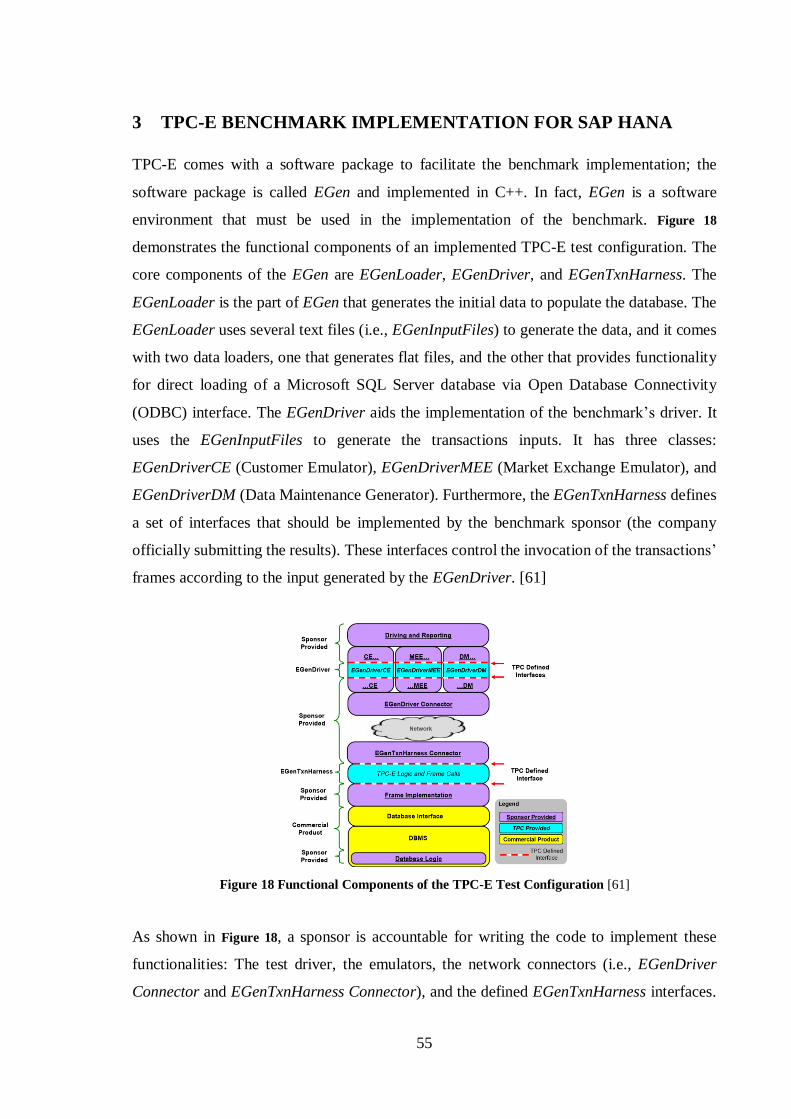
55
3 TPC-E BENCHMARK IMPLEMENTATION FOR SAP HANA
TPC-E comes with a software package to facilitate the benchmark implementation; the
software package is called EGen and implemented in C++. In fact, EGen is a software
environment that must be used in the implementation of the benchmark. Figure 18
demonstrates the functional components of an implemented TPC-E test configuration. The
core components of the EGen are EGenLoader, EGenDriver, and EGenTxnHarness. The
EGenLoader is the part of EGen that generates the initial data to populate the database. The
EGenLoader uses several text files (i.e., EGenInputFiles) to generate the data, and it comes
with two data loaders, one that generates flat files, and the other that provides functionality
for direct loading of a Microsoft SQL Server database via Open Database Connectivity
(ODBC) interface. The EGenDriver aids the implementation of the benchmark’s driver. It
uses the EGenInputFiles to generate the transactions inputs. It has three classes:
EGenDriverCE (Customer Emulator), EGenDriverMEE (Market Exchange Emulator), and
EGenDriverDM (Data Maintenance Generator). Furthermore, the EGenTxnHarness defines
a set of interfaces that should be implemented by the benchmark sponsor (the company
officially submitting the results). These interfaces control the invocation of the transactions’
frames according to the input generated by the EGenDriver. [61]
Figure 18 Functional Components of the TPC-E Test Configuration [61]
As shown in Figure 18, a sponsor is accountable for writing the code to implement these
functionalities: The test driver, the emulators, the network connectors (i.e., EGenDriver
Connector and EGenTxnHarness Connector), and the defined EGenTxnHarness interfaces.
56
The EGenDriver Connector is invoked from the EGenDriver and is responsible for sending
the generated transactions data to, and receiving the corresponding resulting data from, the
EGenTxnHarness Connector through the network. The EGenTxnHarness Connector
receives the transactions data from the EGenDriver Connector and communicates with
EGenTxnHarness via a TPC defined interface. In the same way, the EGenTxnHarness
invokes the sponsor’s implementation of the transactions frame and return the resultant data
to the EGenTxnHarness Connector. [61]
In this work, all of the necessary functionality to be provided by a sponsor to run TPC-E
against SAP HANA are implemented. The benchmark is implemented using C++ and
SQLScript. C++ is used to code the sponsor-provided functionalities while SQLScript is
applied to implement the transactions’ frames. Our TPC-E implementation consists of
almost 11000 lines of C++ code and 2000 lines of SQLScript code. In total, several primary
modules collaborate to provide the functional requirements of the benchmark, as described
in the following subsections.
3.1 Data Loader
An extended database loader is implemented via the EGenLoader. The extended loader can
be employed for generating the flat files, bulk importing from the flat files into HANA or a
combination of both operations. Data generation and data import are separated to provide
more flexibility since the data generation is time-consuming and can be done only once.
The data generation is implemented by using the CGenerateAndLoad class shipped with the
EGenLoader. The class delivers routines for generating and loading the data tables which
among them we used only the data generation interfaces. The data generation can be
configured by command line arguments to generate fixed, scaling, growing tables or a
mixture of them.
The data import is completed in five stages. First, the tables are generated in a schema called
TPCE. In HANA, databases can be divided into logical sub-databases known as a schema.
After generating the TPCE schema, the loader imports the delimited flat files using IMPORT
FROM statement supported by HANA. Then, the TPC-E referential integrity constraints are
57
enforced at the third step. Afterwards, several indexes are generated to speed up the search
operations. Finally, the transactions’ procedures are created in the database. The data loader
uses HANA ODBC driver to communicate with the DBMS.
3.2 Common Functionalities
There are several functionalities in the benchmark which are shared between the driver and
Tier A (the application layer). The common functionalities can be classified into multi-
tasking, networking, and logging features. This section briefly explains the design principles
and architectural choices applied to them.
Firstly, some parts of the benchmark demand parallel execution. For example, a multi-
threading architecture is necessary for replicating CEs and MEEs as single instances of the
customer emulator and market exchange emulator can achieve a limited throughput
compared to the nominal throughput. The job execution framework of the HANA DBMS
kernel is utilized for thread pooling and running job nodes. The job execution framework is
NUMA-aware and exploits task scheduling to prevent CPU saturation. The classes that
define job nodes follow a naming convention; the job node classes end with a ‘JobNode’
postfix like DMJobNode, CEJobNode, and MEEJobNode. The job node classes should
inherit from a base class and implement a pure virtual function named run. The run function
contains the code that needs to be executed as a parallel task.
As mentioned before, TPC-E demands a mandatory network layer between the driver and
the Tier A. Two class named CNetworkServer and CClientConnector are implemented to
handle streaming data over network sockets. The CClientConnector is the class used for
transmitting transaction requests and transaction orders over the network (from driver to the
Tier A, and from the Tier A to MEE server). SendReqReceiveResp is the method
implemented for sending the requests and receiving the response. Before the transmission,
the transactions are serialized into a union data type. CNetworkServer class is responsible
for receiving the request from the network client, processing the request, and sending back
the results. The network server class uses synchronous data transfer architecture; however,
a job is executed upon receiving each request to prevent blocking concurrent requests. The
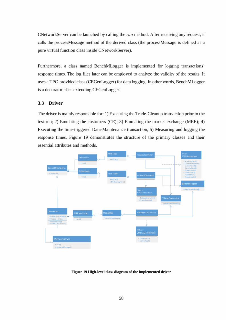
58
CNetworkServer can be launched by calling the run method. After receiving any request, it
calls the processMessage method of the derived class (the processMessage is defined as a
pure virtual function class inside CNetworkServer).
Furthermore, a class named BenchMLogger is implemented for logging transactions’
response times. The log files later can be employed to analyze the validity of the results. It
uses a TPC-provided class (CEGenLogger) for data logging. In other words, BenchMLogger
is a decorator class extending CEGenLogger.
3.3 Driver
The driver is mainly responsible for: 1) Executing the Trade-Cleanup transaction prior to the
test-run; 2) Emulating the customers (CE); 3) Emulating the market exchange (MEE); 4)
Executing the time-triggered Data-Maintenance transaction; 5) Measuring and logging the
response times. Figure 19 demonstrates the structure of the primary classes and their
essential attributes and methods.
BenchTPCERunner
+ startRun()
CEJobNode
+run()
DMJobNode
+run()
CMEEServer
#meeQeue : Queue
+ProcessMessage()
CNetworkServer
+ run()
CClientConnector
+ SendReqReceiveResp ()
MEEJobNode
+run()
TPCE::CMEESutInterface
+ BrokerVolume()
HDBMEESUTConnector
TPCE::CMEESUTInterface
+ TradeResult()
TPCE::CCE
+ doTxn()
TPCE::CDM
+ doTxn()
TPCE:CMEE
+submitTradeRequest()
HDBCESUTConnector
HDBDMSUTConnector
TPCE::CDMSutInterface
+ DataMaintenance()
+startMEEJobExecutor()
+ processMessage()
BenchMLogger
+ logElapsedTime()
+ CustomerPosition()+ MarketWatch()+ SecurityDetail()+ TradeLookup()+ TradeOrder()+ TradeStatus()+ TradeUpdate()
+ TradeCleanup()
+ MarketFeed()
+ DoCleanupTxn()
# mutex : Mutex
Figure 19 High-level class diagram of the implemented driver
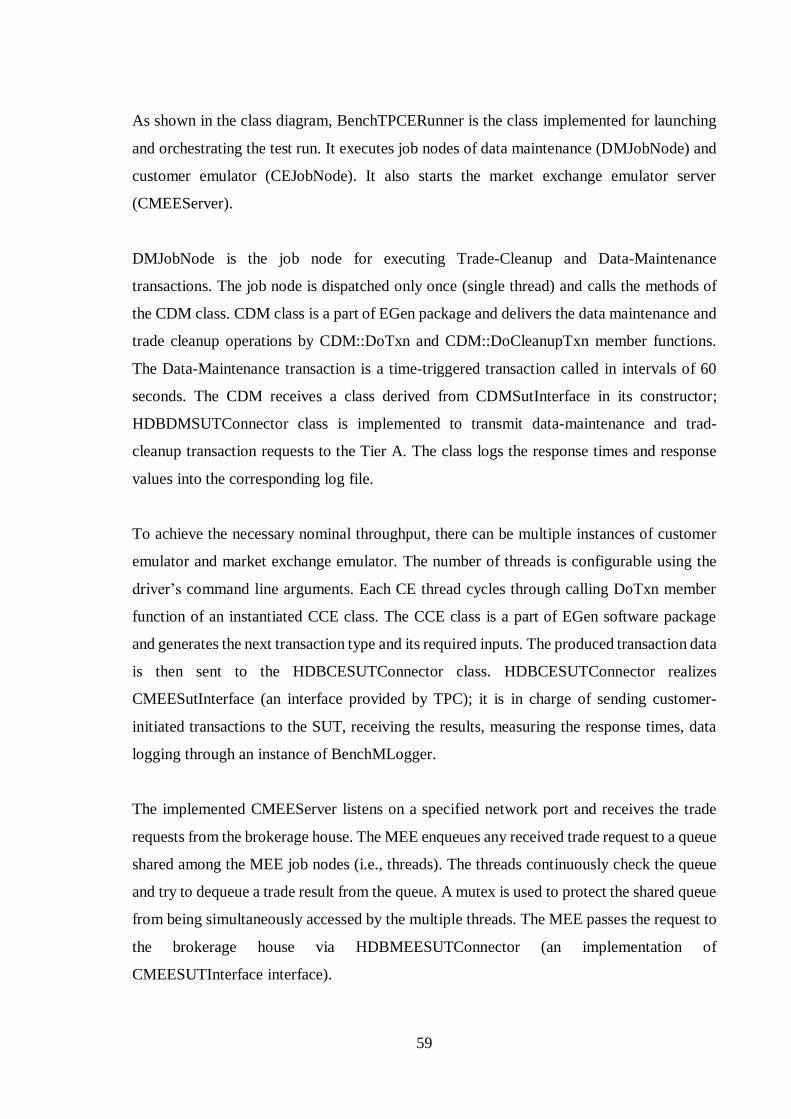
59
As shown in the class diagram, BenchTPCERunner is the class implemented for launching
and orchestrating the test run. It executes job nodes of data maintenance (DMJobNode) and
customer emulator (CEJobNode). It also starts the market exchange emulator server
(CMEEServer).
DMJobNode is the job node for executing Trade-Cleanup and Data-Maintenance
transactions. The job node is dispatched only once (single thread) and calls the methods of
the CDM class. CDM class is a part of EGen package and delivers the data maintenance and
trade cleanup operations by CDM::DoTxn and CDM::DoCleanupTxn member functions.
The Data-Maintenance transaction is a time-triggered transaction called in intervals of 60
seconds. The CDM receives a class derived from CDMSutInterface in its constructor;
HDBDMSUTConnector class is implemented to transmit data-maintenance and trad-
cleanup transaction requests to the Tier A. The class logs the response times and response
values into the corresponding log file.
To achieve the necessary nominal throughput, there can be multiple instances of customer
emulator and market exchange emulator. The number of threads is configurable using the
driver’s command line arguments. Each CE thread cycles through calling DoTxn member
function of an instantiated CCE class. The CCE class is a part of EGen software package
and generates the next transaction type and its required inputs. The produced transaction data
is then sent to the HDBCESUTConnector class. HDBCESUTConnector realizes
CMEESutInterface (an interface provided by TPC); it is in charge of sending customer-
initiated transactions to the SUT, receiving the results, measuring the response times, data
logging through an instance of BenchMLogger.
The implemented CMEEServer listens on a specified network port and receives the trade
requests from the brokerage house. The MEE enqueues any received trade request to a queue
shared among the MEE job nodes (i.e., threads). The threads continuously check the queue
and try to dequeue a trade result from the queue. A mutex is used to protect the shared queue
from being simultaneously accessed by the multiple threads. The MEE passes the request to
the brokerage house via HDBMEESUTConnector (an implementation of
CMEESUTInterface interface).

60
3.4 Tier A
Figure 20 shows the structure of the primary classes and their important attributes and
methods used in the Tier A (also called application layer). CTxnHarnessConnector is
primarily accountable for listening on a specific network port. The class inherits from
CNetworkServer; it checks the transaction type upon receiving any customer-initiated or
market-triggered transaction. Subsequently, CTxnHarnessConnector instantiates a TPC-
provided class corresponding to the requested transaction. The instantiated classed can be of
types: CBrokerVolume, CCustomerPosition, CDataMaintenance, CMarketFeed,
CMarketWatch, CSecurityDetail, CTradeCleanup, CTradeLookup, CTradeOrder,
CTradeResult, CTradeStatus, or CTradeUpdate. Any of these classes requires implementing
a class conforming a specific interface. For instance, CBrokerVolume requires an
implementation of CBrokerVolumeDBInterface (HdbBrokerVolume in our
implementation). The classes in the class diagram starting with “Hdb” are implementations
for specific interfaces. The Hdb-starting classes receive transactions’ inputs, bind stored
procedures’ parameters, and call the equivalent stored procedure using ODBC. Finally, the
Hdb-starting classes return transactions output to CTxnHarnessConnector. The stored
procedures are implements in SQLScript language (see section 2.4.4). In total, 30 stored
procedures incorporate the benchmark’s transactions.
As shown in the application layer’s class diagram, two classes (i.e., CMarketFeed and
CTradeOrder) contain references to CSendToMarket class. The CSendToMarket class
inherits from CClientConnector and CSendToMarketInterface; it controls sending trade
requests to market exchange emulator server (via SendToMarket member function) through
the network.
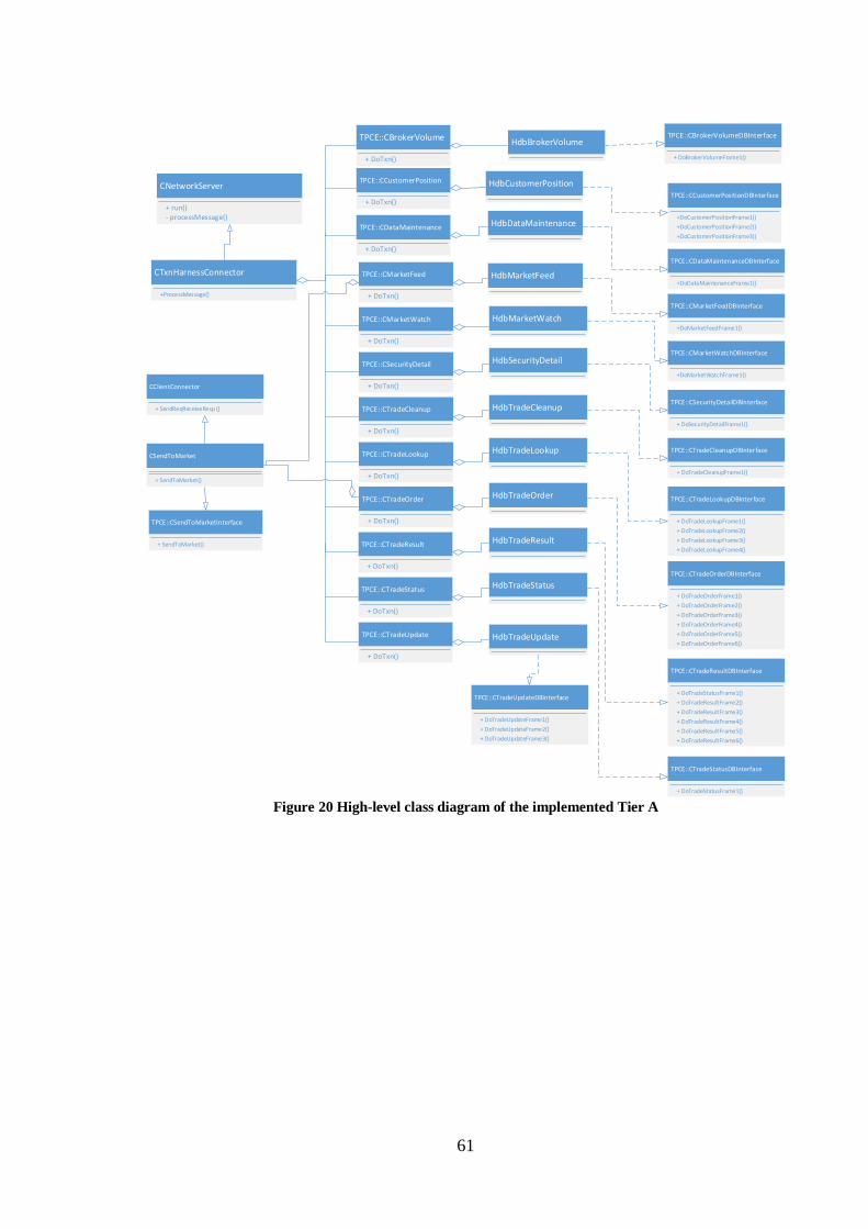
61
CTxnHarnessConnector
+ProcessMessage()
CNetworkServer
+ run()- processMessage()
TPCE::CBrokerVolumeDBInterface
+ DoBrokerVolumeFrame1()
HdbCustomerPositionTPCE::CCustomerPositionDBInterface
+DoCustomerPositionFrame1()
+DoCustomerPositionFrame2()
+DoCustomerPositionFrame3()
HdbDataMaintenance
TPCE::CDataMaintenanceDBInterface
+DoDataMaintenanceFrame1()HdbMarketFeed
TPCE::CMarketFeedDBInterface
+DoMarketFeedFrame1()
HdbMarketWatch
TPCE::CMarketWatchDBInterface
+DoMarketWatchFrame1()
HdbSecurityDetail
TPCE::CSecurityDetailDBInterface
+ DoSecurityDetailFrame1()
HdbTradeCleanup
TPCE::CTradeCleanupDBInterface
+ DoTradeCleanupFrame1()
HdbTradeLookup
TPCE::CTradeLookupDBInterface
+ DoTradeLookupFrame1()
+ DoTradeLookupFrame2()
+ DoTradeLookupFrame3()
+ DoTradeLookupFrame4()
HdbTradeOrder
TPCE::CTradeOrderDBInterface
+ DoTradeOrderFrame1()
+ DoTradeOrderFrame2()
+ DoTradeOrderFrame3()
+ DoTradeOrderFrame4()
+ DoTradeOrderFrame5()
+ DoTradeOrderFrame6()
HdbTradeResult
TPCE::CTradeResultDBInterface
+ DoTradeStatusFrame1()
+ DoTradeResultFrame2()
+ DoTradeResultFrame3()
+ DoTradeResultFrame4()
+ DoTradeResultFrame5()
+ DoTradeResultFrame6()
HdbTradeStatus
TPCE::CTradeStatusDBInterface
+ DoTradeStatusFrame1()
HdbTradeUpdate
TPCE::CTradeUpdateDBInterface
+ DoTradeUpdateFrame1()
+ DoTradeUpdateFrame2()
+ DoTradeUpdateFrame3()
CSendToMarket
+ SendToMarket()
TPCE::CSendToMarketInterface
+ SendToMarket()
CClientConnector
+ SendReqReceiveResp ()
HdbBrokerVolumeTPCE::CBrokerVolume
+ DoTxn()
TPCE::CCustomerPosition
+ DoTxn()
TPCE::CDataMaintenance
+ DoTxn()
TPCE::CMarketFeed
+ DoTxn()
TPCE::CMarketWatch
+ DoTxn()
TPCE::CSecurityDetail
+ DoTxn()
TPCE::CTradeCleanup
+ DoTxn()
TPCE::CTradeLookup
+ DoTxn()
TPCE::CTradeOrder
+ DoTxn()
TPCE::CTradeResult
+ DoTxn()
TPCE::CTradeStatus
+ DoTxn()
TPCE::CTradeUpdate
+ DoTxn()
Figure 20 High-level class diagram of the implemented Tier A

62
4 EXPERIMENT
This section explores the experiment’s results. First, the underlying experiment
configuration is provided including the database management system and the hardware.
Then, the benchmark is run against both row and columnar data stores to answer RQ1.
Afterwards, the results of profiling are provided to explore RQ2. Finally, SQLScript is
evaluated for OLTP workload (RQ3).
4.1 Experiment Configuration
4.1.1 Database Management System
To launch the benchmark, a research version of SAP HANA 2 is used as the underlying
database management system. In the experiment, the benchmark is configured with 20000
customers (see section 2.5.3 for a detailed explanation about scaling the benchmark). The
reason for selecting 20000 customers is that higher number of customers demand complex
hardware configurations (e.g., a server cluster with multiple terabytes of memory).
Furthermore, data generation and import become significantly time-consuming while the
number of customers increases. Also, a configuration with 20000 provides an acceptable
initial database size. An initial trade days (ITD) of 300 days and a scale factor (SF) of 500
are used for data generation. Table 5 shows the initial cardinality of tables after the database
population.
In total, the generated data for the database population amounts to 142 GB of raw flat files.
The initial database size for storing the generated data in the columnar layout (aka column
store) is 51 GB, and the initial size for storing the same data in the row-wise layout (aka row
store) is 151 GB. The initial database size is the allocated space for storing all database
entities including data, indexes, and database metadata [63]. Even though both the row-store
and column store employ compression mechanisms to save space, the column store achieves
a significant space saving compared to the row store (a factor of 2.96). This implicates the
benefits of the columnar layout regarding memory saving as explained in section 2.2.4.

63
Table Cardinality Table Cardinality
ACCOUNT_PERMISSION 141.979 INDUSTRY 102
ADDRESS 30.004 LAST_TRADE 13.700
BROKER 200 NEWS_ITEM 20.000
CASH_TRANSACTION 317.950.537 NEWS_XREF 20.000
CHARGE 15 SECTOR 12
COMMISION_RATE 240 SECURITY 13.700
COMPANY 10.000 SETTLEMENT 345.600.000
COMPANY_COMPETITOR 30.000 STATUS_TYPE 5
CUSTOMER 20.000 TAXRATE 320
CUSTOMER_ACCOUNT 100.000 TRADE 345.600.000
CUSTOMER_TAXRATE 40.000 TRADE_HISTORY 829.434.764
DAILY_MARKET 17.878.500 TRADE_REQUEST 0
EXCHANGE 4 TRADE_TYPE 5
FINANCIAL 200.000 WATCH_ITEM 1.999.003
HOLDING 17.664.875 WATCH_LIST 20.000
HOLDING_HISTORY 463.172.112 ZIP_CODE 14.741
HOLDING_SUMMARY 993.000
Table 5 Initial cardinality of tables
4.1.2 Underlying Hardware
A single server is utilized to execute the benchmark; the driver, Tier A, and Tier B share
hardware resources. The server has four 10-core processors Intel Xeon Processor E7-4870
at 2.40 GHz; in total, 80 hardware contexts are supported using hyper-threading. Each core
has 32 KB L1d (i.e., L1 data cache), 32 KB L1i (i.e., L1 instruction cache), and 256 KB of
L2 cache. Besides, each processor employs 30 MB of L3 cache that is shared among its
cores. The processors incorporate four NUMA nodes (each node includes ten cores). Also,
the server has 512 GB of RAM and 5.7 TB of rotating disks.
The operating system (OS) installed on the server is a 64-bit SUSE Linux Enterprise Server
12 with service pack 1 (SP1). The operating system runs a 3.12 Linux kernel.
4.2 Throughput Evaluation
The evaluation is run in two primary stages. First, the column store engine of HANA is used
to evaluate the achievable throughput. Then, the benchmark is executed against the row store
engine. The gained throughput is measure in tpsE (see section 2.5.3). Due to confidentiality
concerns and SAP legal policies, we cannot disclose the absolute throughputs; the achieved

64
throughputs are normalized to a percent. This does not hinder us from presenting results of
the experiment since the focus is on comparing the performance of the data stores.
As discussed in section 3.3, the implemented driver receives the number of CEs and MEEs
from the command line. This helps us to configure the number of threads to replicate
customer emulators and market exchange emulators to generate the necessary nominal
throughput for database size with 20000 customers. The nominal throughput for a database
with 20000 customers is 40 tpsE (2.00 tpsE for every 1000 customers). Also, the measured
throughput for such a database sizing must be in the range of 32 tpsE and 40.8 tpsE (80 to
102 percent of the nominal throughput) according to the benchmark rules. Hence, the test is
executed multiple times to find the number of threads necessary to achieve an acceptable
measured throughput for the column store. During the experiment, a single instance of the
driver configured with 35 threads of CE and five threads of MEE is used. The throughput
evaluation incorporates several critical steps, as follows.
1. The flat files are generated.
2. The column store is populated via the data loader.
3. The benchmark is performed against the columnar engine to measure its throughput.
Each test run takes 140 minutes: one-minute ramp-up, 138 minutes of the
measurement interval, and one-minute ramp-down. The test is repeated five times to
achieve verifiable results. The throughput expressed in this thesis is the average of
the five test-runs.
4. The row store is populated using the loader.
5. The procedure explained in step 3 is executed for the row store.
The steps explained above will aid understanding how an in-memory columnar HTAP
perform with OLTP workload comparing to the row store (RQ1).
4.2.1 Achieved Throughput and Response-times
As shown in Figure 21, the row-store engine outperforms the column-store engine for the
OLTP workload with a 26% difference; the normalized throughput of the column-store is

65
74% of the achieved throughput for the row-store engine. The x-axis in the figure shows the
achieved throughput in a percent scale.
Figure 21 measured throughputs of the row-store and column-store engines
While both test runs (column and row store engines) maintain the ninetieth percentile of the
required response times, the valid response times are measured for two groups of
transactions: read-only and read-write transactions. Figure 22 and Figure 23 render box plots
of the response times per individual transactions for column store and row store engine. The
y-axis in the figures sketches response times (log scale) while the x-axis includes boxes
representing transactions grouped into the column and row store. The ends of the whiskers
show the minimum and maximum response times. The bottom and top of the boxes show
first and third quartiles, whereas the bands inside the boxes denote the medians. Also, the
Trade-Cleanup transaction is omitted since it is executed only once at the beginning of the
test run and does not affect the throughput.
Figure 22 Response times of the read-only transactions
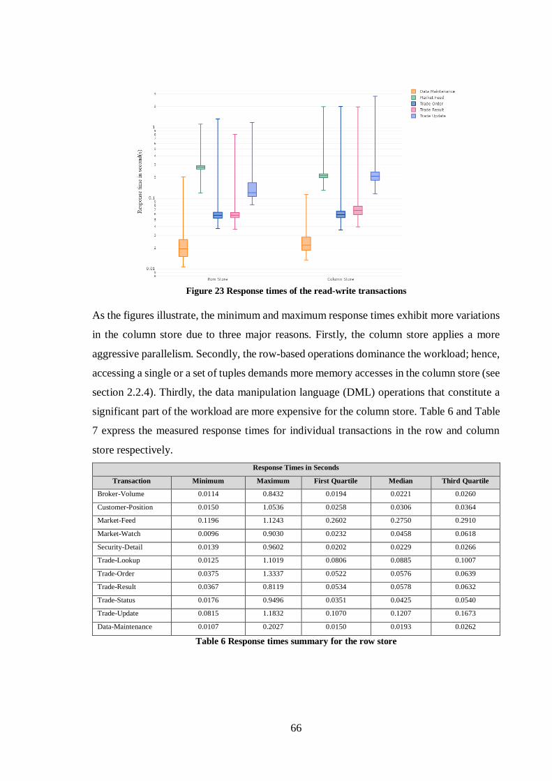
66
Figure 23 Response times of the read-write transactions
As the figures illustrate, the minimum and maximum response times exhibit more variations
in the column store due to three major reasons. Firstly, the column store applies a more
aggressive parallelism. Secondly, the row-based operations dominance the workload; hence,
accessing a single or a set of tuples demands more memory accesses in the column store (see
section 2.2.4). Thirdly, the data manipulation language (DML) operations that constitute a
significant part of the workload are more expensive for the column store. Table 6 and Table
7 express the measured response times for individual transactions in the row and column
store respectively.
Response Times in Seconds
Transaction Minimum Maximum First Quartile Median Third Quartile
Broker-Volume 0.0114 0.8432 0.0194 0.0221 0.0260
Customer-Position 0.0150 1.0536 0.0258 0.0306 0.0364
Market-Feed 0.1196 1.1243 0.2602 0.2750 0.2910
Market-Watch 0.0096 0.9030 0.0232 0.0458 0.0618
Security-Detail 0.0139 0.9602 0.0202 0.0229 0.0266
Trade-Lookup 0.0125 1.1019 0.0806 0.0885 0.1007
Trade-Order 0.0375 1.3337 0.0522 0.0576 0.0639
Trade-Result 0.0367 0.8119 0.0534 0.0578 0.0632
Trade-Status 0.0176 0.9496 0.0351 0.0425 0.0540
Trade-Update 0.0815 1.1832 0.1070 0.1207 0.1673
Data-Maintenance 0.0107 0.2027 0.0150 0.0193 0.0262
Table 6 Response times summary for the row store

67
Response Times in Seconds
Transaction Minimum Maximum First Quartile Median Third Quartile
Broker-Volume 0.0118 1.9577 0.0188 0.0214 0.0255
Customer-Position 0.0150 2.7597 0.0251 0.0414 0.0729
Market-Feed 0.1301 1.9863 0.1966 0.2093 0.2229
Market-Watch 0.0171 2.0236 0.0338 0.0585 0.0701
Security-Detail 0.0163 2.1202 0.0245 0.0274 0.0316
Trade-Lookup 0.0159 2.2371 0.0961 0.1087 0.1221
Trade-Order 0.0358 1.9998 0.0535 0.0591 0.0658
Trade-Result 0.0396 1.9734 0.0590 0.0680 0.0778
Trade-Status 0.0328 0.9983 0.0643 0.0724 0.0826
Trade-Update 0.1159 2.7909 0.1811 0.2073 0.2363
Data-Maintenance 0.0133 0.1134 0.0185 0.0219 0.0283
Table 7 Response times summary for the column store
Next section inspects how the workload breaks down into main components of HANA.
4.3 Profiling Results
HANA architecture consists of several servers; index server is one of the core components
among them. The index-server consists of the in-memory data stores and data processing
engines. During the test runs, a profiler embedded in HANA is employed as an instrument
to collect information about the performance of the index server. The profiler operates by
sampling the index server’s call-stacks at regular intervals. Using the profiler assist us in
analyzing the call stacks and the processor time spent in individual function calls as well as
identifying wait conditions. The output of the profiler is two graphs created via DOT [64]
language: a wait graph and a processor utilization graph. Consequently, the profiling results’
contributions are twofold. First, it assists analyzing how OLTP workloads breakdown into
key components of an HTAP system (RQ2). Second, the results aid identifying the
bottlenecks affecting the benchmark throughput.
The whole profiler graphs are not provided here since they are huge and cannot be fit in the
text size. However, an excerpt of the profiling graph is given in Figure 24. Each node in the
graph represents a process/function, and each edge denotes the calling relationship between
a caller and a callee. The graph nodes include two numbers: ‘I’ is an abbreviation for
inclusive time and ‘E’ stand for exclusive time. The inclusive time is the amount of processor
time used by a function including the time spent in the child functions. On the other hand,

68
the exclusive time shows the amount of time spent purely in a function excluding the child
functions. Also, the numbers next to the arrows show the percentage of CPU time spent in
the child functions. Moreover, the more reddish boxes express the higher processor time
spent in a function. In the figure, ptime::Query::_execute is the query execution function
taking almost 62 percent of the total CPU time. It calls ptime::proc_update_trex::operator
(the function responsible for SQL update statement), ptime::proc_delete_trex::operator (the
function corresponding to SQL delete statement), and ptime::proc_insert_trex::operator
(the function applying SQL insert statement). By looking at the graph, it can be understood
that 6.8% of the processor time is taken for DML operations (4.4% update + 1% delete +
1.4% insert). The main findings of the profiling process are explained in the next subsections.
Figure 24 An excerpt of the profile graph for the column store

69
4.3.1 Workload Decomposition
The benchmark’s workload breakdown is shown in Figure 25 and Figure 26 for the column
store and the row store. Only the main cost drivers are included in the charts because the
focus is on the key drivers (miscellaneous costs are shown as others in the figures). The key
drivers are classified into sorting operation, data store access and predicate evaluation,
memory management, DML operations, query compilation and validation, network transfer
and communication, SQLScript execution and overhead, and index access and join
processing.
Figure 25 Workload breakdown for the row store engine
Sorting Operation8%
Data Store Access and Predicate Evaluation
14%
Memory Management11%
DML Operations6%
Query Compilation and Validation
15%
Network Transafer and Communication
12%
SQLScript Execution and Overhead
4%
Index Access and Join Processing
13%
Others17%
Sorting Operation Data Store Access and Predicate Evaluation
Memory Management DML Operations
Query Compilation and Validation Network Transafer and Communication
SQLScript Execution and Overhead Index Access and Join Processing
Others
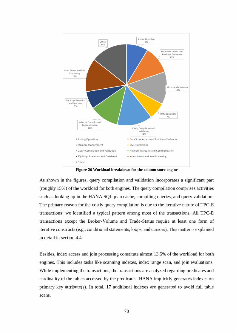
70
Figure 26 Workload breakdown for the column store engine
As shown in the figures, query compilation and validation incorporates a significant part
(roughly 15%) of the workload for both engines. The query compilation comprises activities
such as looking up in the HANA SQL plan cache, compiling queries, and query validation.
The primary reason for the costly query compilation is due to the iterative nature of TPC-E
transactions; we identified a typical pattern among most of the transactions. All TPC-E
transactions except the Broker-Volume and Trade-Status require at least one form of
iterative constructs (e.g., conditional statements, loops, and cursors). This matter is explained
in detail in section 4.4.
Besides, index access and join processing constitute almost 13.5% of the workload for both
engines. This includes tasks like scanning indexes, index range scan, and join evaluations.
While implementing the transactions, the transactions are analyzed regarding predicates and
cardinality of the tables accessed by the predicates. HANA implicitly generates indexes on
primary key attribute(s). In total, 17 additional indexes are generated to avoid full table
scans.
Sorting Operation9%
Data Store Access and Predicate Evaluation
11%
Memory Management13%
DML Operations7%
Query Compilation and Validation
14%
Network Transafer and Communication
12%
SQLScript Execution and Overhead
7%
Index Access and Join Processing
13%
Others14%
Sorting Operation Data Store Access and Predicate Evaluation
Memory Management DML Operations
Query Compilation and Validation Network Transafer and Communication
SQLScript Execution and Overhead Index Access and Join Processing
Others

71
Also, data-store access and predicate evaluation is another cost driver of the experiment
workload. The store access and predicate evaluation take 11.1% of the total processor time
for the column store and 13.8% for the row store. This includes both sargable (i.e., predicates
that could take advantage of indexes to accelerate query execution) and non-sargable
predicates.
Furthermore, 13% of the CPU time is spent in memory management for the column store.
The memory management takes 10.8% of the processor time for the row store. HANA
utilizes a memory manager which pre-allocate and manages memory pools. Memory
management mostly consists of memory allocation and deallocation. It is worth mentioning
that the memory management and query compilation costs are intertwined; the less query
compilation decreases the overhead of memory allocation.
Besides, network transfer and communication is also a key part consuming 11.6% of the
processor time for the column store and 12.3% for the row store. This includes accepting
new network connections, session management, and data transfer.
Furthermore, almost nine percent of the total processor time is spent for sorting operations
during the benchmark run (8.7% for the column store and 8% for the row store). This can be
justified by the fact that majority of the transactions (all except Market-Watch) include at
least one ORDER BY clause (for intermediate tables and/or final results).
In addition, DML handling constitutes 6.8% of the workload for the column store and 6.2%
for the row store. This includes insert, update, and delete operations. Finally, execution of
the SQLScript procedures and the overhead of the execution (e.g., converting arguments,
binding intermediate results to internal tables, and creating contexts to store data globally)
incorporate 7% of the total workload for the column store and 4.1% for the row store engine.
72
4.3.2 Checkpointing and Recovery
HANA uses a persistence layer server to store a persistent copy of data and transaction logs;
they ensure database recovery after failures such as crashes and power loss. In HANA, all
changed pages are persisted to disk periodically (called savepoint or checkpoint). However,
the periodical savepoints by themselves cannot guarantee the durability of all changes since
persistence is not synchronized with the end of write transactions. Hence, the system stores
log files (redo logs and undo information); the redo log contains committed changes while
the undo log stores entries about rolled-back changes. The log entries are persisted while a
transaction is committed or rolled-back. [65]
During a recovery process, HANA performs a log replay process upon the last version of the
persisted data to store database to a consistent state. It should be mentioned that the recovery
process is possible even without running checkpoints since logs can be replayed upon the
initial version of the persistent data (the version of data loaded into memory). Nevertheless,
periodical save-points accelerate the recovery process because fewer log entries must be
replayed. The checkpointing interval is by default 300 seconds, yet it can be configured or
even disabled. [65]
The checkpointing in HANA includes three stages: A page-flush, a critical, and a post-
critical phase. During the page-flush, all modified pages are identified and written to disk.
Next, all changes made throughout the page-flush stage are written to disk asynchronously
in the critical phase. Also, the current log position is altered and stored on disk through the
critical phase. While running the critical phase, all concurrent update transactions are
blocked. Lastly, the post-critical phase waits for finishing all the asynchronous I/O
operations and marks the save-point as complete. [65]
In the initial runs of the benchmark, it was found out that the checkpointing process causes
fluctuations during the benchmark’s steady state. Thus, the checkpointing interval is changed
in several steps to understand effects of the checkpointing on the test run. First, the
benchmark is run with checkpointing every five minutes as shown in Figure 27. The x-axis
in the figure shows the elapsed time while the y-axis demonstrates the achieved throughput
(the throughput is normalized to 100). Then, the checkpointing interval is increased to ten

73
minutes (see Figure 28). Afterwards, the checkpointing interval is expanded to 60 minutes
as can be seen in Figure 29. Finally, Figure 30 exhibits the experiment run graph while
checkpointing is disabled. The graphs manifest running experiment on the row store, yet, the
instabilities also exist with the column store.
Figure 27 Experiment run graph with checkpointing at intervals of 5-minute
Figure 28 Experiment run graph with checkpointing at intervals of 10-minute
0
20
40
60
80
100
120
00:0
0:0
0
00:0
4:0
0
00:0
8:0
0
00:1
2:0
0
00:1
6:0
0
00:2
0:0
0
00:2
4:0
0
00:2
8:0
0
00:3
2:0
0
00:3
6:0
0
00:4
0:0
0
00:4
4:0
0
00:4
8:0
0
00:5
2:0
0
00:5
6:0
0
01:0
0:0
0
01:0
4:0
0
01:0
8:0
0
01:1
2:0
0
01:1
6:0
0
01:2
0:0
0
01:2
4:0
0
01:2
8:0
0
01:3
2:0
0
01:3
6:0
0
01:4
0:0
0
01:4
4:0
0
01:4
8:0
0
01:5
2:0
0
01:5
6:0
0
02:0
0:0
0
02:0
4:0
0
02:0
8:0
0
02:1
2:0
0
02:1
6:0
0
02:2
0:0
0
Checkpointing Interval : 5 Minutes
0
20
40
60
80
100
120
00:0
0:0
0
00:0
4:0
0
00:0
8:0
0
00:1
2:0
0
00:1
6:0
0
00:2
0:0
0
00:2
4:0
0
00:2
8:0
0
00:3
2:0
0
00:3
6:0
0
00:4
0:0
0
00:4
4:0
0
00:4
8:0
0
00:5
2:0
0
00:5
6:0
0
01:0
0:0
0
01:0
4:0
0
01:0
8:0
0
01:1
2:0
0
01:1
6:0
0
01:2
0:0
0
01:2
4:0
0
01:2
8:0
0
01:3
2:0
0
01:3
6:0
0
01:4
0:0
0
01:4
4:0
0
01:4
8:0
0
01:5
2:0
0
01:5
6:0
0
02:0
0:0
0
02:0
4:0
0
02:0
8:0
0
02:1
2:0
0
02:1
6:0
0
Checkpointing Interval : 10 Minutes

74
Figure 29 Experiment run graph with checkpointing at intervals of 60-minute
Figure 30 Experiment run graph while checkpointing is disabled
The figures validate implication of the checkpoints on the experiment. To begin with, the
number of variations drops by enlarging the checkpoint intervals; though, the duration of the
fluctuations increase since more changes must be synchronized each time. Also, the
fluctuations are diminished by disabling the checkpoints.
The throughputs explained in section 4.2 are measured without checkpointing. The
checkpointing issues mostly stem from poor I/O performance; the underlying server used for
0
20
40
60
80
100
120
00:0
0:0
0
00:0
4:0
0
00:0
8:0
0
00:1
2:0
0
00:1
6:0
0
00:2
0:0
0
00:2
4:0
0
00:2
8:0
0
00:3
2:0
0
00:3
6:0
0
00:4
0:0
0
00:4
4:0
0
00:4
8:0
0
00:5
2:0
0
00:5
6:0
0
01:0
0:0
0
01:0
4:0
0
01:0
8:0
0
01:1
2:0
0
01:1
6:0
0
01:2
0:0
0
01:2
4:0
0
01:2
8:0
0
01:3
2:0
0
01:3
6:0
0
01:4
0:0
0
01:4
4:0
0
01:4
8:0
0
01:5
2:0
0
01:5
6:0
0
02:0
0:0
0
02:0
4:0
0
02:0
8:0
0
02:1
2:0
0
02:1
6:0
0
Checkpointing Interval : 60 Minutes
0
20
40
60
80
100
120
00:0
0:0
0
00:0
4:0
0
00:0
8:0
0
00:1
2:0
0
00:1
6:0
0
00:2
0:0
0
00:2
4:0
0
00:2
8:0
0
00:3
2:0
0
00:3
6:0
0
00:4
0:0
0
00:4
4:0
0
00:4
8:0
0
00:5
2:0
0
00:5
6:0
0
01:0
0:0
0
01:0
4:0
0
01:0
8:0
0
01:1
2:0
0
01:1
6:0
0
01:2
0:0
0
01:2
4:0
0
01:2
8:0
0
01:3
2:0
0
01:3
6:0
0
01:4
0:0
0
01:4
4:0
0
01:4
8:0
0
01:5
2:0
0
01:5
6:0
0
02:0
0:0
0
02:0
4:0
0
02:0
8:0
0
02:1
2:0
0
02:1
6:0
0
Disabled Checkpointing
75
the experiment employs rotating disks. Consequently, using more performant non-volatile
storages like solid-state drive (SSD) might alleviate the issue. However, future work is
needed to establish this. At the time, SAP is adopting non-volatile RAM (called NVRAM or
NVM) technologies like Intel 3D XPoint in HANA’s architecture [66]. There is room for
further research in determining how using the NVRAM technologies could alleviate the
throughput variations during the experiment.
4.4 SQLScript Evaluation for OLTP Workload
Relational databases traditionally offer imperative language extensions using a dialect of
SQL such as Procedural Language/Structured Query Language(PL/SQL), Transact-SQL(T-
SQL), and SQLScript [60]. Even though the offered iterative extensions ease pushing
application logic to the database, performance requirements also of concern while using such
constructs. The performance requirements play a crucial factor for OLTP workloads. In this
section, it is explored how optimal an HTAP-oriented stored procedure language like
SQLScript is for OLTP workloads (RQ3).
During the experiment, it was found out that query compilation and validation is one of the
major cost drivers while running the benchmark (roughly 15% of the total processor time).
Therefore, this matter was investigated in a greater detail, and the iterative nature of TPC-E
transactions turned out to be the primary reason of the costly query compilations. We
identified a typical pattern among most of the transactions; all TPC-E transactions except
the Broker-Volume and Trade-Status require at least one form of iterative constructs (e.g.,
conditional statements, loops, and cursors). Put it differently, SQLScript provides a
suboptimal performance for queries of this kind. In some situations, iterative-approach can
be converted to a set-based logic; however, this is not always possible. For instance, FOR
loops containing dependent SQL statements are less probable to be converted into a set-
based logic. Hence, it was decided to produce a simplified version of the situation and
examine our theory using it.
Two exemplified transactions are built on top of TPC-E schema called L1 and L2. L1 and
L2 access four tables of TPC-E schema as shown in Figure 31. The only change made to the
TPC-E schema is dropping the primary key from the TRADE_HISTORY table since it is
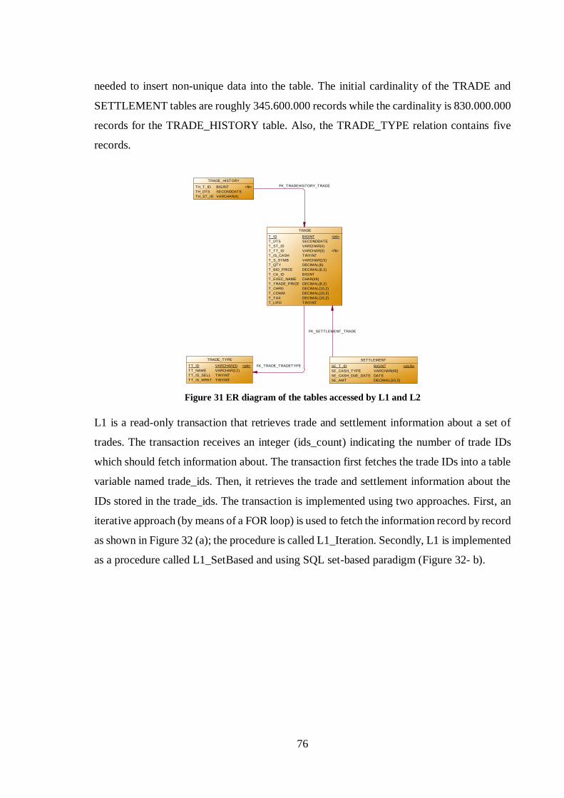
76
needed to insert non-unique data into the table. The initial cardinality of the TRADE and
SETTLEMENT tables are roughly 345.600.000 records while the cardinality is 830.000.000
records for the TRADE_HISTORY table. Also, the TRADE_TYPE relation contains five
records.
Figure 31 ER diagram of the tables accessed by L1 and L2
L1 is a read-only transaction that retrieves trade and settlement information about a set of
trades. The transaction receives an integer (ids_count) indicating the number of trade IDs
which should fetch information about. The transaction first fetches the trade IDs into a table
variable named trade_ids. Then, it retrieves the trade and settlement information about the
IDs stored in the trade_ids. The transaction is implemented using two approaches. First, an
iterative approach (by means of a FOR loop) is used to fetch the information record by record
as shown in Figure 32 (a); the procedure is called L1_Iteration. Secondly, L1 is implemented
as a procedure called L1_SetBased and using SQL set-based paradigm (Figure 32- b).
FK_SETTLEMENT_TRADE
FK_TRADE_TRADETYPE
FK_TRADEHISTORY_TRADE
SETTLEMENT
SE_T_ID
SE_CASH_TYPE
SE_CASH_DUE_DATE
SE_AMT
BIGINT
VARCHAR(40)
DATE
DECIMAL(10,2)
<pk,fk>
TRADE
T_ID
T_DTS
T_ST_ID
T_TT_ID
T_IS_CASH
T_S_SYMB
T_QTY
T_BID_PRICE
T_CA_ID
T_EXEC_NAME
T_TRADE_PRICE
T_CHRG
T_COMM
T_TAX
T_LIFO
BIGINT
SECONDDATE
VARCHAR(4)
VARCHAR(3)
TINYINT
VARCHAR(15)
DECIMAL(6)
DECIMAL(8,2)
BIGINT
CHAR(49)
DECIMAL(8,2)
DECIMAL(10,2)
DECIMAL(10,2)
DECIMAL(10,2)
TINYINT
<pk>
<fk>
TRADE_HISTORY
TH_T_ID
TH_DTS
TH_ST_ID
BIGINT
SECONDDATE
VARCHAR(4)
<fk>
TRADE_TYPE
TT_ID
TT_NAME
TT_IS_SELL
TT_IS_MRKT
VARCHAR(3)
VARCHAR(12)
TINYINT
TINYINT
<pk>

77
CREATE PROCEDURE L1_Iteration(IN ids_count INT)
LANGUAGE SQLSCRIPT AS
BEGIN DECLARE i INT;
DECLARE trade_ids TABLE(tid BIGINT);
DECLARE trade_id BIGINT;
trade_ids = SELECT TOP : ids_count T_ID as tid FROM TRADE;
FOR i IN 1.. ids_count DO
trade_id = :trade_ids.tid[:i];
SELECT T_BID_PRICE, T_EXEC_NAME, T_IS_CASH,
TT_IS_MRKT, T_TRADE_PRICE
FROM TRADE, TRADE_TYPE WHERE T_ID = :trade_id
AND T_TT_ID = TT_ID;
SELECT SE_AMT, SE_CASH_DUE_DATE, SE_CASH_TYPE
FROM SETTLEMENT WHERE SE_T_ID = :trade_id;
END FOR;
END;
CREATE PROCEDURE L1_SetBased(IN ids_count INT)
LANGUAGE SQLSCRIPT AS
BEGIN DECLARE i INT;
DECLARE trade_ids TABLE(id BIGINT);
trade_ids = SELECT TOP : ids_count T_ID as id FROM TRADE;
SELECT T_BID_PRICE, T_EXEC_NAME, T_IS_CASH,
TT_IS_MRKT, T_TRADE_PRICE
FROM TRADE, TRADE_TYPE WHERE T_ID in
(select id from :trade_ids) AND T_TT_ID = TT_ID;
SELECT SE_AMT, SE_CASH_DUE_DATE, SE_CASH_TYPE
FROM SETTLEMENT WHERE SE_T_ID in
(select id from :trade_ids);
END;
(a) (a)
Figure 32 (a) L1 implementation using iterative constructs, (b) L1 implementation using a set-based approach
In addition, L2 is a read-write transaction that updates timestamp of the trades (T_DTS) and
inserts the updated trade information into the TRADE_HISTORY table. Just like L1, the
transaction receives an integer (ids_count) expressing the number of trades which have to be
updated. The transaction is implemented using three styles. First, an iterative approach (by
a FOR loop) is used to retrieve the information record by record as shown in Figure 33(a);
the procedure is called L2_Iteration. The L2_Iteration procedure performs L2 in a single-
tuple-at-a-time fashion; SELECT, UPDATE, and INSERT operations are iteratively
performed in a loop. Furthermore, another implementation of L2 is provided in Figure 33(b).
The procedure is named L2_Mixed and differs from L2_Iteration in the way it handles
UPDATE operations; IDs of the trades are stored in a table variable (inserts_itab), and the
update operation is executed in a single execution. Finally, the L2_SetBased procedure
(Figure 33 - c) performs L2 using a SQL set-based approach (Figure 32- b).

78
CREATE PROCEDURE L2_Iteration(IN ids_count INT,
OUT updated INT, OUT inserted INT)
LANGUAGE SQLSCRIPT AS
BEGIN
DECLARE now_dts SECONDDATE;
DECLARE i INT;
DECLARE tid BIGINT;
updated = 0;
inserted = 0;
now_dts = NOW();
FOR i IN 1.. ids_count DO
SELECT TOP 1 T_ID INTO tid FROM TPCE."TRADE"
WHERE T_DTS != :now_dts;
UPDATE TPCE."TRADE" SET T_DTS = :now_dts WHERE
T_ID = :tid;
updated = updated + ::ROWCOUNT;
INSERT INTO TPCE."TRADE_HISTORY"
(TH_T_ID, TH_DTS, TH_ST_ID)
VALUES(tid, :now_dts, 'SBMT');
inserted = inserted + ::ROWCOUNT;
SELECT tid from dummy;
END FOR;
COMMIT;
END;
CREATE PROCEDURE L2_Mixed(IN ids_count INT,
OUT updated INT, OUT inserted INT)
LANGUAGE SQLSCRIPT AS
BEGIN
DECLARE now_dts SECONDDATE;
DECLARE i INT;
DECLARE tid BIGINT;
DECLARE inserts_itab TABLE(id BIGINT, dts SECONDDATE,
status VARCHAR(4));
updated = 0;
inserted = 0;
now_dts = NOW();
FOR i IN 1.. ids_count DO
SELECT TOP 1 T_ID INTO tid FROM TPCE."TRADE"
WHERE T_DTS != :now_dts;
UPDATE TPCE."TRADE" SET T_DTS = :now_dts WHERE
T_ID = :tid;
updated = updated + ::ROWCOUNT;
:inserts_itab.insert((:tid, :now_dts, 'SBMT'));
END FOR;
INSERT INTO TPCE."TRADE_HISTORY"(TH_T_ID, TH_DTS,
TH_ST_ID) SELECT id, dts, status FROM :inserts_itab;
inserted = inserted + ::ROWCOUNT;
COMMIT;
SELECT id from :inserts_itab;
END;
(a) (b) CREATE PROCEDURE L2_SetBased(IN ids_count INT, OUT updated INT, OUT inserted INT) LANGUAGE SQLSCRIPT AS
BEGIN
DECLARE now_dts SECONDDATE;
DECLARE i INT;
DECLARE trades TABLE(id BIGINT, dts SECONDDATE, status VARCHAR(4));
updated = 0;
inserted = 0;
now_dts = NOW();
trades = SELECT TOP : ids_count T_ID as id, :now_dts as dts, 'SBMT' as status FROM TPCE."TRADE" WHERE T_DTS != :now_dts;
UPDATE TPCE."TRADE" SET T_DTS = :now_dts WHERE T_ID in (SELECT id from :trades);
updated = updated + ::ROWCOUNT;
INSERT INTO TPCE."TRADE_HISTORY"(TH_T_ID, TH_DTS, TH_ST_ID) SELECT id, dts, status FROM :trades;
inserted = inserted + ::ROWCOUNT;
COMMIT;
SELECT id from :trades;
END;
(c) Figure 33 (a) L2 implementation using iterative constructs, (b) L2 implementation using a mixed approach, (c)
L2 implementation using a set-based approach
The L1 and L2 procedures are called with an increasing sequence of ids_count to
comprehend how the procedures differ in connection with response times. It also facilitates
understanding how increasing the ids_count correspond with the procedures’ response times.
A client application is implemented using C++ to execute the procedures and measure
response times. To achieve verifiable results, each procedure is called 100 times and the
average response time is reported.

79
Figure 34 portrays how the procedures performed in respect of response time. The x-axis
characterizes a sequence of ids_count (number of trade IDs). The y-axis describes the
response times (log2 scale). It is apparent from the figure that L1_SetBased and
L2_SetBased outperform their counterparts. The set-based procedures also excel regarding
the growth rate. While the running times for the procedures using iterative constructs
increase almost linearly in relation to ids_count, the L1_SetBased and L2_SetBased grow at
a sub-linear scale. Besides, despite the fact that L2_Mixed executes fewer SQL statements
inside the loop (INSERT statement is done in a single execution), there is no significant
difference between the performance of L2_Iteration and L2_Mixed.
Figure 34 L1 and L2 response times
The profiling tool explained in section 4.3 is applied to compare cost drivers while executing
the L1_Iteration and L1_SetBased. It is shown that query compilation cost is orders of
magnitudes higher for L1_Iteration; query compilation takes 4.5% and 19.5% of CPU
service time for L1_SetBased and L1_Iteration respectively. The query compilation also
affects memory management costs. The L1_Iteration takes 17% process time for memory
allocation and deallocation while the costs are almost zero for L1_SetBased. The results
validate our theory about the connection between query compilation cost and the iterative
nature of TPC-E transactions. Accordingly, we strongly believe that the experiment’s
throughput and workload decomposition dramatically improves if the benchmark
transactions are converted to set-based approach.
1
2
4
8
16
32
64
128
256
512
1024
2048
1 2 4 8 16 32 64 128 256 512 1024
Res
ponse
Tim
e
ids_count
L1_Iteration
L1_SetBased
L2_Iteration
L2_SetBased
L2_Mixed

80
Application logic is becoming more complex, and it is not always possible to implement the
logic only via native SQL statements. To this end, languages like SQLScript could be
equipped with some mechanisms converting imperative logic to pure SQL statements during
query optimization. This is an important issue for future research; one optimization approach
can be converting iterative SQL queries into SQL nested queries and set-based operation
(like what is done in L1_SetBased and L2_SetBased manually) during query compilation
and optimization. This also might require a dependence analysis (data dependency and
control dependency) to determine whether operations inside iterative constructs can be un-
nested or unrolled. To this end, some studies [67, 68, 69] have been conducted to analyze
identifying batch-safe iterations and replacing imperative loops with single batch calls. This
impovement is picked up for future HANA development efforts.
81
5 CONCLUSION
5.1 Scope and Background
Typically, the “one size does not fit all” has been the dominant paradigm used to separate
OLTP and OLAP data into different database management systems. Even though the
separation could be advantageous, it also gives rise to several deficiencies like data
redundancy and lack of real-time analytics. To blur boundaries between analytical and
transactional data management systems, some disruptive approaches have been taken toward
building HTAP systems. HTAP systems mostly rely on in-memory computation to present
profound performance improvements. In addition, columnar data layout has become popular
mainly for OLAP use-cases.
The primary goal of this thesis is evaluating the performance of an in-memory HTAP system
using a columnar data layout with OLTP workload. Firstly, it investigates how a columnar
HTAP perform with transactional workload comparing to a row-wise data storage (RQ1).
Secondly, the thesis examines the main cost drivers of OLTP workload in an HTAP system
(RQ2). Thirdly, it studies how optimal an HTAP-oriented stored procedure language
(SQLScript) is for OLTP workloads (RQ3). To answer the research questions, a systematic
literature review is combined with a quantitative experimental research. A research version
of SAP HANA is used as the underlying HTAP system during the experiment. Also, an
industry-grade OLTP benchmark (TPC-E) is implemented to generate the needed workload
for the research.
Studies on the performance of columnar databases have mostly focused on OLAP and mixed
workloads [55, 70, 71, 72, 73, 74, 75]. However, far little attention has been paid to how
column-oriented data layout perform with pure transactional processing. For instance, a
study by D.J. Abadi, S.R. Madden and N. Hachem [70] has compared the performance of a
column store database with several row-store systems using star schema benchmark
(SSMB), a data warehousing benchmark. Likewise, A. Kemper and T. Neumann [71] have
used a mixed workload benchmark (TPC-CH) to compare the performance of an HTAP
system supporting columnar data layout, HyPer, with several OLTP and OLAP-oriented
databases. Similarly, I. Psaroudakis et al. [55] investigate the performance of two HTAP
82
systems with a mixed workload benchmark (CH-benCHmark). In the same way, Z. Feng et
al. in their study [72] assess the performance of data scan and lookup operations in an in-
memory column store with TPC-H (a decision support benchmark provided by TPC). Also,
the study conducted by E. Petraki, S. Idreos and S. Manegold [73] measures the performance
of an indexing mechanism for column-oriented database architectures via TPC-H. In the
same manner, I. Alagiannis, M. Athanassoulis and A. Ailamaki [74] utilize TPC-H and SSB
(two analytical benchmarks) to analyze scaling up queries with column stores. J. Wang et al.
[75] analyze the performance of a column store SQL engine with a TPC-H like benchmark
as well. Hence, the thesis tries to fill the gap between the performance of columnar HTAP
systems and transactional workload.
Besides, very few studies have investigated and applied TPC-E benchmark [76, 62, 77]. This
is also the dominant trend in the industry, and the benchmark results have been published
only for one DBMS (Microsoft SQL Server) [78]. This matter could stem from complex
nature of the benchmark comparing to the other OLTP benchmarks such as TPC-C. TPC-E
incorporates a three-tier architecture and requires a complex code base (our TPC-E
implementation consists of almost 11000 lines of C++ code). Also, TPC-E transactions
exhibit elaborate structures (roughly 2000 lines of SQLScript code in our implementation).
TPC-E also demands sophisticated DBMS requirements such as referential integrity
constraints and the highest ANSI transaction isolation level (i.e., serializability). Using TPC-
E workload in this thesis aids achieving results representing requirements of a modern OLTP
environment.
5.2 Main Findings
To evaluate the performance of an in-memory columnar data management system for OLTP
workload, TPC-E benchmark is run against both the row and columnar data engines
embedded in HANA. The column store exhibits more fluctuations regarding the
transactions’ response times due to three major reasons. Firstly, the column store engine
applies a more aggressive parallelism. Secondly, the row-based operations dominance the
benchmark workload, hence, accessing a single or a set of tuples demands more memory
accesses in the column store. Thirdly, DML operations that constitute a significant part of
the workload are more expensive for the column store. Despite the variations, our experiment
83
shows that the column store achieves an acceptable throughput comparing to its counterpart
(the achieved throughput for the column-store is 74% of the row-store throughput).
Therefore, the evidence from this study suggests that the in-memory columnar data
management system can keep up with OLTP use-cases.
Furthermore, a profiling tool is employed to inspect decomposition of the workload into
main HANA components. It is identified that the experiment workload breaks down into
eight primary cost drivers: Query compilation and validation, data store access and predicate
evaluation, memory management, network transfer and communication, index access and
join processing, sorting operation, DML operations, and SQLScript execution.
Among the identified cost drivers, the query compilation and validation constitutes a major
part (roughly 15% of the total processor time). Therefore, this matter was investigated in
greater detail, and the iterative nature of TPC-E transactions turned out to be the primary
reason of the costly query compilations. We identified a typical pattern among most of the
transactions; all TPC-E transactions except the Broker-Volume and Trade-Status require at
least one form of iterative constructs (e.g., conditional statements, loops, and cursors).
Hence, it was decided to produce two simplified transactions (called L1 and L2) and examine
our theory using them. The transactions are implemented using SQLScript in two ways: A
set-based approach and a single-tuple-at-a-time paradigm. The transactions are also utilized
to examine how optimal SQLScript performs for transactional requirements.
Running the profiler on L1 transactions validates our theory about the connection between
query compilation cost and the iterative nature of TPC-E transactions. It is shown that the
query compilation cost is a factor of more than 4X higher for the iterative-based
implementation comparing to the set-based one. The query compilation also affects memory
management costs. Then, the transactions are analyzed regarding the response times and the
growth rates. Running L1 and L2 shows that transactions using SQL set-based operations
outperform those applied iterative constructs in terms of response time and growth rate. Put
it differently, SQLScript provides a suboptimal performance for queries applying iterative
extensions.

84
5.3 Future Work
Some questions remain unanswered and need future research. First, it is found out that
checkpointing causes throughput variations during the experiment. This matter could stem
from the experiment’s underlying hardware configuration; however, future work is needed
to pinpoint the situation. At the time, SAP is adopting non-volatile RAM (called NVRAM
or NVM) technologies like Intel 3D XPoint in HANA’s architecture [66]. There is room for
further research in determining how using the NVRAM technologies could alleviate the
throughput instabilities during the experiment.
Also, further research is required to study the optimization of stored procedures using
iterative paradigm. One optimization approach can be converting iterative SQL queries into
SQL nested queries and set-based operation (like what is done in section 4.4 manually)
during query compilation and optimization. This also might require a dependence analysis
(data dependency and control dependency) to determine whether operations inside iterative
constructs can be un-nested or unrolled. To this end, some studies [67, 68, 69] have been
conducted to analyze identifying batch-safe iterations and replacing imperative loops with
single batch calls. This improvement is picked up for future HANA development efforts.
Moreover, the experiment could be repeated to understand other factors contributing to the
results. First, TPC-E defines 22 check constraints on the benchmark schema; the check
constraints put overhead for DML operations since more operations are required for each
insert, update, and delete statement. Hence, it can be inspected how dropping the constraints
could improve the throughput. Also, the workload breakdown can be analyzed to
comprehend the cost of enforcing the constraints. Secondly, the Trade-Result transaction is
executed with serializable isolation level. The experiment could be further executed with
degrading the isolation level to repeatable read; it is expected that this would improve the
measured throughput since the Trade-Result transactions incorporate 10 percent of the total
workload. Overhead of locking and latching perhaps would go down by changing the
isolation level as well. In addition, the effects of data partitioning on the experiment can be
investigated. No partitioning is used at the current experiment; a further study with more
focus on this matter is therefore suggested. In other words, vertical and horizontal

85
partitioning for the row store, and horizontal partitioning for the column store can be applied
to evaluate how partitioning is in tune with performance optimization.
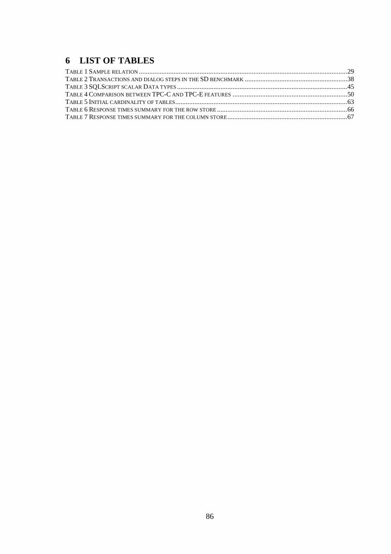
86
6 LIST OF TABLES TABLE 1 SAMPLE RELATION ........................................................................................................................ 29 TABLE 2 TRANSACTIONS AND DIALOG STEPS IN THE SD BENCHMARK ........................................................... 38 TABLE 3 SQLSCRIPT SCALAR DATA TYPES .................................................................................................. 45 TABLE 4 COMPARISON BETWEEN TPC-C AND TPC-E FEATURES .................................................................. 50 TABLE 5 INITIAL CARDINALITY OF TABLES ................................................................................................... 63 TABLE 6 RESPONSE TIMES SUMMARY FOR THE ROW STORE ........................................................................... 66 TABLE 7 RESPONSE TIMES SUMMARY FOR THE COLUMN STORE ..................................................................... 67

87
7 LIST OF FIGURES FIGURE 1 CONCEPTUAL VIEW OF MEMORY HIERARCHY ................................................................................ 15 FIGURE 2 ADVANTAGE OF USING IN-MEMORY DATA MANAGEMENT .............................................................. 16 FIGURE 3 STORAGE PRICE DEVELOPMENT .................................................................................................... 18 FIGURE 4 PROCESSOR DEVELOPMENT ......................................................................................................... 18 FIGURE 5 MEMORY ARCHITECTURE ON INTEL NEHALEM .............................................................................. 23 FIGURE 6 AN EXAMPLE OF MULTIDIMENSIONAL DATA ................................................................................ 27 FIGURE 7 A STAR SCHEMA........................................................................................................................... 28 FIGURE 8 MEMORY ACCESS PATTERN FOR SET-BASED AND ROW-BASED OPERATIONS .................................... 30 FIGURE 9 SAMPLE DATA PARALLELISM ....................................................................................................... 32 FIGURE 10 ACTUAL WORKLOAD IN A MODERN ENTERPRISE APPLICATION ...................................................... 34 FIGURE 11 TPC-C'S BUSINESS ENVIRONMENT .............................................................................................. 35 FIGURE 12 SAMPLE TPC-C RUN GRAPH ....................................................................................................... 37 FIGURE 13 TPC-C ER DIAGRAM OF TABLES AND RELATIONSHIPS AMONG THEM ............................................ 37 FIGURE 14 SD BENCHMARK 2-TIER AND 3-TIER ENVIRONMENT .................................................................... 39 FIGURE 15 MAIN AND DELTA STORAGES IN HANA COLUMNAR LAYOUT ......................................................... 41 FIGURE 16 A PROCEDURAL AND A FUNCTIONAL EXTENSION IN SQLSCRIPT ................................................... 47 FIGURE 17 TPC-E APPLICATION COMPONENTS AND TRANSACTION FLOW ...................................................... 49 FIGURE 18 FUNCTIONAL COMPONENTS OF THE TPC-E TEST CONFIGURATION .............................................. 55 FIGURE 19 HIGH-LEVEL CLASS DIAGRAM OF THE IMPLEMENTED DRIVER ....................................................... 58 FIGURE 20 HIGH-LEVEL CLASS DIAGRAM OF THE IMPLEMENTED TIER A ........................................................ 61 FIGURE 21 MEASURED THROUGHPUTS OF THE ROW-STORE AND COLUMN-STORE ENGINES .............................. 65 FIGURE 22 RESPONSE TIMES OF THE READ-ONLY TRANSACTIONS .................................................................. 65 FIGURE 23 RESPONSE TIMES OF THE READ-WRITE TRANSACTIONS ................................................................. 66 FIGURE 24 AN EXCERPT OF THE PROFILER GRAPH FOR THE COLUMN STORE ................................................... 68 FIGURE 25 WORKLOAD BREAKDOWN FOR THE ROW STORE ENGINE ............................................................... 69 FIGURE 26 WORKLOAD BREAKDOWN FOR THE COLUMN STORE ENGINE ......................................................... 70 FIGURE 27 EXPERIMENT RUN GRAPH WITH CHECKPOINTING AT INTERVALS OF 5-MINUTE ............................... 73 FIGURE 28 EXPERIMENT RUN GRAPH WITH CHECKPOINTING AT INTERVALS OF 10-MINUTE ............................. 73 FIGURE 29 EXPERIMENT RUN GRAPH WITH CHECKPOINTING AT INTERVALS OF 60-MINUTE ............................. 74 FIGURE 30 EXPERIMENT RUN GRAPH WITHOUT CHECKPOINTING ................................................................... 74 FIGURE 31 ER DIAGRAM OF THE TABLES ACCESSED BY L1 AND L2 ............................................................... 76 FIGURE 32 L1 IMPLEMENTATIONS ............................................................................................................... 77 FIGURE 33 L2 IMPLEMENTATIONS ............................................................................................................... 78 FIGURE 34 L1 AND L2 RESPONSE TIMES ....................................................................................................... 79
88
8 REFERENCES
[1] A. Silberschatz, H. F. Korth and S. Sudarshan, Database systems concepts, Estados
Unidos: McGraw-Hill Companies, Inc., 2011.
[2] C. Diaconu, C. Freedman, E. Ismert, P.-A. Larson, P. Mittal, R. Stonecipher, N.
Verma and M. Zwilling, "Hekaton: SQL Serverś Memory-optimized OLTP Engine,"
in Proceedings of the 2013 ACM SIGMOD International Conference on
Management of Data, New York, NY, USA, 2013.
[3] R. Kallman, H. Kimura, J. Natkins, A. Pavlo, A. Rasin, S. Zdonik, E. P. C. Jones, S.
Madden, M. Stonebraker, Y. Zhang, J. Hugg and D. J. Abadi, "H-store: A High-
performance, Distributed Main Memory Transaction Processing System,"
Proceedings of VLDB Endow., vol. 1, pp. 1496-1499, Aug 2008.
[4] S. Idreos, F. Groffen, N. Nes, S. Manegold, K. S. Mullender and M. L. Kersten,
"MonetDB: Two Decades of Research in Column-oriented Database Architectures,"
IEEE Data Engineering Bulletin, vol. 35, pp. 40-45, 2012.
[5] A. Lamb, M. Fuller, R. Varadarajan, N. Tran, B. Vandiver, L. Doshi and C. Bear,
"The Vertica Analytic Database: C-store 7 Years Later," Proceedings of VLDB
Endow., vol. 5, pp. 1790-1801, August 2012.
[6] H. Plattner and A. Zeier, In-Memory Data Management, Berlin, Heidelberg: Springer
Berlin Heidelberg, 2012.
[7] H. Plattner, A Course in In-Memory Data Management, Berlin: Springer Berlin,
2014.
[8] G. P. Copeland and S. N. Khoshafian, "A Decomposition Storage Model," SIGMOD
Rec., vol. 14, pp. 268-279, May 1985.
[9] H. Plattner, "A Common Database Approach for OLTP and OLAP Using an In-
memory Column Database," in Proceedings of the 2009 ACM SIGMOD
International Conference on Management of Data, New York, NY, USA, 2009.
[10] C. D. French, "&Ldquo;One Size Fits All&Rdquo; Database Architectures Do Not
Work for DSS," SIGMOD Rec., vol. 24, pp. 449-450, May 1995.
[11] M. Stonebraker and U. Cetintemel, ""One Size Fits All": An Idea Whose Time Has
Come and Gone," in Proceedings of the 21st International Conference on Data
Engineering, Washington, 2005.
[12] N. May, A. Böhm and W. Lehner, "SAP HANA - The Evolution of an In-Memory
DBMS from Pure OLAP Processing Towards Mixed Workloads," in
Datenbanksysteme für Business, Technologie und Web {(BTW} 2017), Stuttgart,
2017.
[13] A. Kemper and T. Neumann, "HyPer: A Hybrid OLTP&OLAP Main Memory
Database System Based on Virtual Memory Snapshots," in Proceedings of the 2011
IEEE 27th International Conference on Data Engineering, Washington, 2011.
[14] M. Stonebraker and A. Weisberg, "The VoltDB Main Memory DBMS," {IEEE}
Data Eng. Bull., vol. 36, pp. 21-27, 2013.
[15] "Overview of Database Management System," in Fundamentals of Relational
Database Management Systems, Berlin, Heidelberg: Springer Berlin Heidelberg,
2007, pp. 1-30.

89
[16] V. Cuppu, B. Jacob, B. Davis and T. Mudge, "A Performance Comparison of
Contemporary DRAM Architectures," in Proceedings of the 26th Annual
International Symposium on Computer Architecture, Washington, 1999.
[17] H. Garcia-Molina and K. Salem, "Main memory database systems: an overview,"
IEEE Transactions on Knowledge and Data Engineering, vol. 4, pp. 509-516,
December 1992.
[18] J. Lindström, V. Raatikka, J. Ruuth, P. Soini and K. Vakkila, "IBM solidDB: In-
Memory Database Optimized for Extreme Speed and Availability," {IEEE} Data
Eng. Bull., vol. 36, pp. 14-20, 2013.
[19] T. J. Lehman, E. J. Shekita and L.-F. Cabrera, "An Evaluation of Starburstś Memory
Resident Storage Component," IEEE Trans. on Knowl. and Data Eng., vol. 4, pp.
555-566, December 1992.
[20] H. Lu, Y. Y. Ng and Z. Tian, "T-Tree or B-Tree: Main Memory Database Index
Structure Revisited," in Proceedings of the Australasian Database Conference,
Washington, 2000.
[21] D. J. DeWitt, R. H. Katz, F. Olken, L. D. Shapiro, M. R. Stonebraker and D. A.
Wood, "Implementation Techniques for Main Memory Database Systems," SIGMOD
Rec., vol. 14, pp. 1-8, June 1984.
[22] V. Sikka, F. Färber, W. Lehner, S. K. Cha, T. Peh and C. Bornhövd, "Efficient
Transaction Processing in SAP HANA Database: The End of a Column Store Myth,"
in Proceedings of the 2012 ACM SIGMOD International Conference on
Management of Data, New York, NY, USA, 2012.
[23] T. Lahiri, M.-A. Neimat and S. Folkman, "Oracle TimesTen: An In-Memory
Database for Enterprise Applications," {IEEE} Data Eng. Bull., vol. 36, pp. 6-13,
2013.
[24] J. L. Hennessy and D. A. Patterson, Computer Architecture, Fourth Edition: A
Quantitative Approach, San Francisco, CA, USA: Morgan Kaufmann Publishers Inc.,
2006.
[25] J. Levandoski, "Modern Main-Memory Database Systems," 2016.
[26] K.-Y. Whang and R. Krishnamurthy, "Query Optimization in a Memory-resident
Domain Relational Calculus Database System," ACM Trans. Database Syst., vol. 15,
pp. 67-95, March 1990.
[27] P. Pucheral, J.-M. Thévenin and P. Valduriez, "Efficient Main Memory Data
Management Using the DBgraph Storage Model," in Proceedings of the Sixteenth
International Conference on Very Large Databases, San Francisco, CA, USA, 1990.
[28] T. J. Lehman and M. J. Carey, "A Recovery Algorithm for a High-performance
Memory-resident Database System," SIGMOD Rec., vol. 16, pp. 104-117, December
1987.
[29] K. Salem and H. Garcia-Molina, "System M: a transaction processing testbed for
memory resident data," IEEE Transactions on Knowledge and Data Engineering,
vol. 2, pp. 161-172, March 1990.
[30] V. Leis, A. Kemper and T. Neumann, "The Adaptive Radix Tree: ARTful Indexing
for Main-memory Databases," in Proceedings of the 2013 IEEE International
Conference on Data Engineering (ICDE 2013), Washington, 2013.
90
[31] T. J. Lehman and M. J. Carey, "A Study of Index Structures for Main Memory
Database Management Systems," in Proceedings of the 12th International
Conference on Very Large Data Bases, San Francisco, CA, USA, 1986.
[32] J. J. Levandoski, D. B. Lomet and S. Sengupta, "The Bw-Tree: A B-tree for New
Hardware Platforms," in Proceedings of the 2013 IEEE International Conference on
Data Engineering (ICDE 2013), Washington, 2013.
[33] G. Graefe and W. J. McKenna, "The Volcano Optimizer Generator: Extensibility and
Efficient Search," in Proceedings of the Ninth International Conference on Data
Engineering, Washington, 1993.
[34] T. Neumann, "Efficiently Compiling Efficient Query Plans for Modern Hardware,"
Proceedings of VLDB Endow., vol. 4, pp. 539-550, Jun 2011.
[35] D. Porobic, I. Pandis, M. Branco, P. Tözün and A. Ailamaki, "OLTP on Hardware
Islands," Proceedings of VLDB Endow., vol. 5, pp. 1447-1458, #jul# 2012.
[36] F. Färber, S. K. Cha, J. Primsch, C. Bornhövd, S. Sigg and W. Lehner, "SAP HANA
Database: Data Management for Modern Business Applications," SIGMOD Rec., vol.
40, pp. 45-51, Jan 2012.
[37] J. Gray and A. Reuter, Transaction Processing: Concepts and Techniques, 1st ed.,
San Francisco, CA, USA: Morgan Kaufmann Publishers Inc., 1992.
[38] M. H. Eich, "A classification and comparison of main memory database recovery
techniques," in 1987 IEEE Third International Conference on Data Engineering,
1987.
[39] M. H. Eich, "Mars: The Design of a Main Memory Database Machine," in Database
Machines and Knowledge Base Machines, M. Kitsuregawa and H. Tanaka, Eds.,
Boston, MA: Springer US, 1988, pp. 325-338.
[40] N. Malviya, A. Weisberg, S. Madden and M. Stonebraker, "Rethinking main memory
OLTP recovery," in 2014 IEEE 30th International Conference on Data Engineering,
2014.
[41] P. A. Boncz, M. L. Kersten and S. Manegold, "Breaking the Memory Wall in
MonetDB," Commun. ACM, vol. 51, pp. 77-85, December 2008.
[42] A. Thomson and D. J. Abadi, "Modularity and Scalability in Calvin," {IEEE} Data
Eng. Bull., vol. 36, pp. 48-55, 2013.
[43] P. A. Bernstein and E. Newcomer, Principles of Transaction Processing, 2nd ed., San
Francisco, CA, USA: Morgan Kaufmann Publishers Inc., 2009.
[44] M. T. Ozsu, Principles of Distributed Database Systems, 3rd ed., Upper Saddle
River, NJ, USA: Prentice Hall Press, 2007.
[45] E. F. Codd, S. B. Codd and C. T. Salley, Providing OLAP (On-line Analytical
Processing) to User-analysts: An IT Mandate, Codd & Associates, 1993.
[46] S. Chaudhuri and U. Dayal, "An Overview of Data Warehousing and OLAP
Technology," SIGMOD Rec., vol. 26, pp. 65-74, Mar 1997.
[47] H. Plattner and B. Leukert, The In-Memory Revolution: How SAP HANA Enables
Business of the Future, Springer Publishing Company, Incorporated, 2015.
[48] F. Özcan, Y. Tian and P. Tözün, "Hybrid Transactional/Analytical Processing: A
Survey," in Proceedings of the 2017 ACM International Conference on Management
of Data, New York, NY, USA, 2017.

91
[49] I. Psaroudakis, T. Scheuer, N. May and A. Ailamaki, "Task Scheduling for Highly
Concurrent Analytical and Transactional Main-Memory Workloads," in International
Workshop on Accelerating Data Management Systems Using Modern Processor and
Storage Architectures - {ADMS} 2013, Riva del Garda, Trento, Italy, August 26,
2013., 2013.
[50] J. Krueger, C. Kim, M. Grund, N. Satish, D. Schwalb, J. Chhugani, H. Plattner, P.
Dubey and A. Zeier, "Fast Updates on Read-optimized Databases Using Multi-core
CPUs," Proceedings of VLDB Endow., vol. 5, pp. 61-72, September 2011.
[51] K. Shanley, "History and Overview of the TPC," Transaction Processing
Performance Council, February 1998. [Online]. Available:
http://www.tpc.org/information/about/history.asp.
[52] "TPC Benchmark C Standard Specification Revision 5.11," 2010.
[53] "SAP Standard Application Benchmarks," SAP, [Online]. Available:
https://www.sap.com/about/benchmark.html. [Accessed 27 Sep 2017].
[54] "Benchmark Overview SAP SD Standard Application Benchmark," 2015.
[55] I. Psaroudakis, F. Wolf, N. May, T. Neumann, A. Böhm, A. Ailamaki and K.-U.
Sattler, "Scaling Up Mixed Workloads: A Battle of Data Freshness, Flexibility, and
Scheduling," in Performance Characterization and Benchmarking. Traditional to Big
Data: 6th TPC Technology Conference, TPCTC 2014, Hangzhou, China, September
1--5, 2014. Revised Selected Papers, R. Nambiar and M. Poess, Eds., Cham, Springer
International Publishing, 2015, pp. 97-112.
[56] R. Sherkat, C. Florendo, M. Andrei, A. K. Goel, A. Nica, P. Bumbulis, I. Schreter, G.
Radestock, C. Bensberg, D. Booss and H. Gerwens, "Page As You Go: Piecewise
Columnar Access In SAP HANA," in Proceedings of the 2016 International
Conference on Management of Data, New York, NY, USA, 2016.
[57] N. May, W. Lehner, P. Shahul Hameed, N. Maheshwari, C. Müller, S. Chowdhuri
and A. K. Goel, "SAP HANA - From Relational OLAP Database to Big Data
Infrastructure," in {EDBT}, 2015.
[58] N. May, A. Böhm, M. Block and W. Lehner, "Managed Query Processing within the
SAP HANA Database Platform," Datenbank-Spektrum, vol. 15, pp. 141-152, 2015.
[59] "SAP HANA SQLScript Reference," [Online]. Available:
https://help.sap.com/doc/6254b3bb439c4f409a979dc407b49c9b/2.0.00/en-
US/SAP_HANA_SQL_Script_Reference_en.pdf.
[60] C. Binnig, N. May and T. Mindnich, "SQLScript: Efficiently Analyzing Big
Enterprise Data in SAP HANA," in {BTW}, 2013.
[61] "TPC-E Standard Specification, Revision 1.14.0," 2015.
[62] S. Chen, A. Ailamaki, M. Athanassoulis, P. B. Gibbons, R. Johnson, I. Pandis and R.
Stoica, "TPC-E vs. TPC-C: Characterizing the New TPC-E Benchmark via an I/O
Comparison Study," SIGMOD Rec., vol. 39, pp. 5-10, February 2011.
[63] "TPC-E," TPC, [Online]. Available: http://www.tpc.org/tpce/. [Accessed 05 Oct
2017].
[64] "The DOT Language," [Online]. Available:
http://www.graphviz.org/doc/info/lang.html. [Accessed 23 Nov 2017].

92
[65] "Persistent Data Storage in the SAP HANA Database," SAP, [Online]. Available:
https://help.sap.com/doc/6b94445c94ae495c83a19646e7c3fd56/2.0.01/en-
US/be3e5310bb571014b3fbd51035bc2383.html. [Accessed 24 Nov 2017].
[66] M. Andrei, C. Lemke, G. Radestock, R. Schulze, C. Thiel, R. Blanco, A. Meghlan,
M. Sharique, S. Seifert, S. Vishnoi, D. Booss, T. Peh, I. Schreter, W. Thesing, M.
Wagle and T. Willhalm, "SAP HANA Adoption of Non-volatile Memory,"
Proceedings of VLDB Endow., vol. 10, pp. 1754-1765, August 2017.
[67] K. V. Emani, T. Deshpande, K. Ramachandra and S. Sudarshan, "DBridge:
Translating Imperative Code to SQL," in Proceedings of the 2017 ACM International
Conference on Management of Data, New York, NY, USA, 2017.
[68] R. A. Ganski and H. K. T. Wong, "Optimization of Nested SQL Queries Revisited,"
SIGMOD Rec., vol. 16, pp. 23-33, December 1987.
[69] R. Guravannavar and S. Sudarshan, "Rewriting Procedures for Batched Bindings,"
Proc. VLDB Endow., vol. 1, pp. 1107-1123, #aug# 2008.
[70] D. J. Abadi, S. R. Madden and N. Hachem, "Column-stores vs. Row-stores: How
Different Are They Really?," in Proceedings of the 2008 ACM SIGMOD
International Conference on Management of Data, New York, NY, USA, 2008.
[71] A. Kemper and T. Neumann, "One Size Fits all, Again! The Architecture of the
Hybrid OLTP&OLAP Database Management System HyPer," in Enabling Real-
Time Business Intelligence: 4th International Workshop, BIRTE 2010, Held at the
36th International Conference on Very Large Databases, VLDB 2010, Singapore,
September 13, 2010, Revised Selected Papers, M. Castellanos, U. Dayal and V.
Markl, Eds., Berlin, Heidelberg: Springer Berlin Heidelberg, 2011, pp. 7-23.
[72] Z. Feng, E. Lo, B. Kao and W. Xu, "ByteSlice: Pushing the Envelop of Main
Memory Data Processing with a New Storage Layout," in Proceedings of the 2015
ACM SIGMOD International Conference on Management of Data, New York, NY,
USA, 2015.
[73] E. Petraki, S. Idreos and S. Manegold, "Holistic Indexing in Main-memory Column-
stores," in Proceedings of the 2015 ACM SIGMOD International Conference on
Management of Data, New York, NY, USA, 2015.
[74] I. Alagiannis, M. Athanassoulis and A. Ailamaki, "Scaling Up Analytical Queries
with Column-stores," in Proceedings of the Sixth International Workshop on Testing
Database Systems, New York, NY, USA, 2013.
[75] J. Wang, H. Duan, G. Min, G. Ying and S. Zheng, "Goldfish: In-Memory Massive
Parallel Processing SQL Engine Based on Columnar Store," in
iThings/GreenCom/CPSCom/SmartData, 2016.
[76] Y. Li and C. Levine, "Extending TPC-E to Measure Availability in Database
Systems," in Topics in Performance Evaluation, Measurement and Characterization:
Third TPC Technology Conference, TPCTC 2011, Seattle, WA, USA, August 29-
September 3, 2011, Revised Selected Papers, R. Nambiar and M. Poess, Eds., Berlin,
Heidelberg: Springer Berlin Heidelberg, 2012, pp. 111-122.
[77] R. O. Nascimento and P. R. M. Maciel, "DBT-5: An Open-Source TPC-E
Implementation for Global Performance Measurement of Computer Systems,"
Computing and Informatics, vol. 29, pp. 719-740, 2010.

93
[78] "TPC-E - All Results," TPC, [Online]. Available:
http://www.tpc.org/tpce/results/tpce_results.asp. [Accessed 02 11 17].


![[]Oracle® Enterprise Manager Cloud Control …Analytic In-Memory Database withAdaptive In-Memory Caching and Columnar Compression. Optimized InfiniBand connectivity to Oracle Exadata.](https://static.fdocuments.us/doc/165x107/5f5afec3349652609c2deb99/oracle-enterprise-manager-cloud-control-analytic-in-memory-database-withadaptive.jpg)