EU’s Preferential Trade Agreements With Developing ... · Draft version, do not quote EU’s...
30
Draft version, do not quote EU’s Preferential Trade Agreements With Developing Countries Revisited Luis Verdeja † † Ph.D Candidate at the University of Nottingham, School of Ecnonomics
Transcript of EU’s Preferential Trade Agreements With Developing ... · Draft version, do not quote EU’s...

Draft version, do not quote
EU’s Preferential Trade Agreements With Developing Countries Revisited
Luis Verdeja†
† Ph.D Candidate at the University of Nottingham, School of Ecnonomics
1
1. INTRODUCTIONThe European Union (EU) has a long history of non-reciprocal preferential trade
agreements with developing countries.‡ For almost 40 years, since the signature of
Yaoundé I in 1963, the EU has constantly enlarged the scope of these agreements and
today over 140 countries benefit from some form of preferential access to the EU market.
The main schemes through which the EU has put in place this policy have been the
Lomé Convention and the Generalized System of Preferences (GSP). The former grants
preferential access to European markets to a group of 78 African, Caribbean and Pacific
states (ACP) and the latter to over 140 low and medium income countries spread all over
the world. §
However, in the past ten years, the EU has begun to consider a change in its trade
strategy with ACP countries. Among the reasons for this change is the failure to
integrate ACP countries in the world economy. The extension of this argument is that
the Lomé Convention has failed in its purpose of boosting ACP economies through
trade. Consequently, it would be reasonable to conclude that non-reciprocal preferential
access has been ineffective in promoting ACP exports.
Given that the Lomé Convention is the most comprehensive preferential trade
agreement granted by the EU, other systems like the GSP should work no better. This, in
turn raises the question of whether preferential trade agreements have been (and
continue to be) beneficial for developing countries or not.
In spite of this change in policy with ACP countries, the EU has continued to show
its belief in preferential treatment and in 2000 launched the Everything But Arms (EBA)
Initiative, which grants quota and duty free access to the European market to all Least
Developed Countries (LDCs).
In this paper we intend to analyze whether trade preferences have actually been
beneficial to developing countries (and are a good policy option) by studying the last 30
years of exports to the EU from a large sample of trading partners, including both
developing and developed economies. Our analysis builds on the work of Nilsson (2002)
‡ In strict legal terms, the body which has the legal capacity to sign agreements is the European
Communities. However, since the European Union remains the more widely known term we use the latter throughout the article.

2
who, using a gravity model, found that both the Lomé Convention and the GSP had a
positive impact on the beneficiary countries. Interestingly enough, there are very few
studies evaluating the exporting capacity of ACP, GSP and MED countries using a
gravity setting.
In the last decades the gravity model has become one of the most popular devices
to analyze trade flows.** In its basic form, the gravity equation predicts trade flows as a
function of the size of the trade partners and the distance between them. Within this
framework, practically any factor can be controlled for to examine its impact on trade
flows.
The original gravity equation, proposed by Tinbergen (1962), did not have a strong
theoretical foundation.†† In addition, most extensions to the model have used ad hoc
arguments to explain its validity, which makes every result potentially disputable on
economic grounds.‡‡ However many authors have since tried to compensate for this
shortcoming by providing a theoretical foundation to the model. The best known works
are those of Anderson (1979), Bergstrand (1985, 1989) and Deardorff (1995, 1998).
Our intention is to apply the gravity framework to the analysis of these flows.
Consequently, we conduct a number of gravity equations incorporating different
degrees of complexity. Starting from a simple cross-section model replicating Nilsson’s
we then construct a number of panel data gravity models to take into account the new
developments coming both from economic theory and from econometrics. Namely, by
using cross-section models we ignore the importance that prices have in explaining
trade§§ and we create an over restricted model in which we disregard heterogeneity***.
Hence, in addition to the cross-section estimation we discuss the relevance and provide
the results for Pooled Cross Section, Least Squares Dummy Variable, Random Effects
and a two-stage Least Squares estimation as in Cheng and Wall (2004).
§ This includes most ACP countries which in practice do not use this scheme because it is less
comprehensive than Lomé** Rose (2003) says that the gravity model is a completely conventional device used to estimate the
effects of a variety of phenomena on international trade†† Anderson (1979)‡‡ Anderson (2001)§§ See Feenstra (2002)*** See Cheng and Wall (2004)
3
We find that both the Lomé Convention and the GSP scheme had a positive impact
on the exporting capacity of the beneficiary countries in all specifications except in the
two-stage Least Squares, which raises questions about the validity of the GSP scheme.
This finding brings up the issue of whether the EU should move on to a framework of
reciprocity with ACP countries or rather aim for the highest possible degree of non-
reciprocity in the new context envisaged in the Cotonou Agreement.
The remainder of the paper is structured as follows. Section 2 provides an
overview of the history and the relevant trade aspects of the Lomé Convention and the
GSP. Section 3 analyses the causes of the evolution of exports from the relevant regions
to the EU. Section 4 presents the evidence from previous studies on this topic. In Section
5 we develop our model, following the work of Nilsson and provides the justification
and the econometric theory behind the new developments in econometrics. The results
are given and discussed in Section 6 and Section 7 concludes.
2. HISTORY OF EU’S PREFERENTIAL TRADE AGREEMENTSThe EU, driven by an interest to maintain tight economic links with its ex-colonies
and by a sentiment of protection towards them, began soon after the signature of the
Treaty of Rome (1957) to grant preferential access to its market to these recently
independent countries with the objective of promoting their exports and subsequently,
to foster their economic growth. The first of these agreements was the Yaoundé
Convention, which was signed in 1963 between the EU and 18 eighteen ex-colonies,
mostly French.
Ever since, the number of agreements in which the EU conceded some form of
preferential access to its market has been constantly increasing. In 1973, the Lomé
Convention replaced Yaoundé to accommodate the preferences for British ex-colonies,
following the accession of the United Kingdom to the EU. Today, 78 countries from
Africa, Caribbean and the Pacific are signatories of the Lomé Convention. Also in 1973,
the EU signed another preferential trade agreement with Maghreb and Mashreq
countries. In parallel to these regional schemes, the EU started its Generalized System of
Preferences (GSP) in 1971, following the first United Nations Conference on Trade and
Development (UNCTAD). Under the GSP, the EU conceded preferences to 49
developing countries, mostly in manufactures and semi-manufactures, but its non-
4
discriminatory nature, open to almost all developing countries, made that by 1986, 149
countries were covered by the scheme.
However, in the past few years there has been an important change in the way of
facing commercial policy with developing countries, the main difference being that non-
reciprocal preferences will not be granted anymore in a discriminatory way against third
countries, as was foreseen under the Lomé Convention and MED Agreements. The
reasons behind this change are found in two sources. First, the EU has been under
continuous pressure at the World Trade Organization (WTO) for its regional,
preferential agreements. Article XXIV of the WTO allows regional, discriminatory
agreements (i.e. a Free Trade Area) under certain conditions. This violation of the Most
Favored Nation principle is only allowed if the concessions are reciprocal between the
parties of the agreement and/or under the Enabling Clause, which tolerates preferential
agreements only if they are equally offered to all developing countries with the same
level of development. This was not the case of the Lomé and MED agreements, which
were only offered to a limited number of countries and in the end, the EU was forced to
accept their incompatibility with the Enabling Clause and was consequently forced to
phase out these discriminatory preferences.
The second reason is that the Lomé Convention and other non-reciprocal
agreements (notably GSP, and the Mediterranean Agreements) have failed to
significantly promote the exports of developing countries to the EU, which explains the
presence of the political will for change.
Consequently, the EU searched a framework that would allow it to retain its links
with ACP countries and at the same time be compatible with the WTO. This new
framework was put forward with the signature of the Cotonou Agreement in 2000,
replacing the Lomé Conventions, between the EU and the ACP countries. Under such
Agreement, non-reciprocal preferences granted by the EU under Lomé will turn into
different Free Trade Areas (FTAs) that Brussels will negotiate separately with each ACP
region rather than with individual countries. Although some degree of imbalance is
foreseen (initial estimates talk about an almost total product liberalization from the EU
5
and 80% across the different FTAs)††† the move from non-reciprocal to reciprocal trade
agreements is clear. Each of these FTAs will take the name of Economic Partnership
Agreement (EPA) and are due to start in 2008.
This move represents a major change in the economic relationships between the
North and the South. For the first time an FTA will be signed between blocks of such a
different degree of economic development. There are other agreements between
developed and developing countries, such as NAFTA or the EU-Turkey FTA, but none
of them involve so many and so poor countries as the envisaged EPAs.
Before analyzing the performance of these three agreements we need to assess
what we could expect from each of them, because they all contained different
provisions. The most comprehensive and generous of the three was the Lomé
Convention, which entailed the liberalization of 98% of the tariff lines, representing 93%
of total trade.‡‡‡ In fact, the provisions under Lomé were quite generous and the scope of
the preferences granted far larger access than any other non-reciprocal agreement. Other
provisions favoring ACP countries are highlighted in Table A1 in the Appendix.
The preferences granted under other agreements are more modest than under the
Lomé Convention. Langhamer, R. and Sapir, A. (1987) explain that the GSP scheme
provides for duty-quota free access for almost all manufactures and semi-manufactures
(Chapters 25-97 of the Harmonized System except Chapter 93), subject to various
preconditions and within certain product and country specific limits which are fixed
annually. With regard to agricultural products, the number of products included in the
scheme has greatly increased from an initial 155 tariff lines in 1971 (Bormann et al, 1985)
to over 400 in 1999 (Sanchez-Arnau, 2001). Further, some additional concessions have
been made to different groups of countries under the scheme. For instance, those
countries combating drugs receive further preferences in that they face a lower number
of products exempted from the scheme (Andean Pact). The same applies to countries
††† PriceWaterhouse Coopers (2004), financed by and subject to review from the EU, estimates the
impact of the EPAs on ACP countries based on a scenario of 100% liberalization from the EU and 80% from ACP countries. A second scenario of 90% liberalization from both parties was disregarded by Commission officials at a review meeting.
‡‡‡ European Commission (2002)

6
that have implemented selected ILO Conventions or environmental regulations.
Equally, as the UNCTAD (2003) points out, LDCs benefit from increased product
coverage§§§ , rising over to 95% in the period 1998-2002.
3. THE DEBATE ON ACP, GSP AND MED AGREEMENTS
The preferential margin under the Lomé Convention and the GSP scheme has been
estimated in several studies.**** Jadot (2001) estimates a margin favorable to ACP
countries between 0,4% and 4,4%, depending on the ACP region looked at. Another
study, by Hoeckman, Ng and Olarreaga (2001), considers that GSP countries enjoy a
reduction of 3.8 percentage points in the average tariff rate vis a vis Most Favored Nation
(MFN) countries, whereas it increases to 6.5 for ACP countries. This leaves a difference
in the preferential margin of 2.7 points between both schemes.
By its part, he Association Agreements with non-EU Mediterranean countries
provides duty and quota free access for industrial products and those agricultural
products not covered by the CAP.†††† This scheme covers 12 countries, but it has been
upgraded to an FTA for some countries. In fact, in 1995, the process of tightening
economic links between the EU and Mediterranean countries experienced a bold step
forward by with the Barcelona Declaration, that foresees the creation of an FTA with
each MED partner by 2010.
However, this degree of preferential access to the EU has not been reflected in a
positive trend of exports to this market. While one of the aims of Lomé was to increase
the market share of ACP exports in the EU, it has actually declined from 6,7 per cent in
1976 to 2,8 percent in 1998 of total imports (EC, 2003). Even though the total amount of
exports to the EU has increased, it has done it in a timid way, allowing for the overall
loss in their market share.
Indeed, it seems that the impact of the Lomé Conventions on the exporting
performance of ACP countries has been very limited. Only a handful of them have
§§§ Product coverage is defined as products covered over dutiable imports**** See UNCTAD (2003), Sánchez Arnau (2001) or Bormann et al (1985) for different ways of
estimating the margins.†††† Pelkmans (2001)

7
Graph 1. Market Share of EU Imports from Relevant Region
0
5
10
15
20
25
30
35
40
45
73-74 75-77 78-80 81-83 84-86 87-89 90-92 93-95 96-98 99-00Years
Per
cen
t
GSP
ACP
ACP w/o S.Africa
MED
Source: OECD, own calculationsSource: OECD, own calculationsSource: OECD, own calculations
experienced sustained growth rates over the average of developing countries (Messerlin,
2001). Even so, most of the successful countries have been so because they benefited
from the different protocols, which are probably the most discriminatory aspects of the
Lomé Convention.‡‡‡‡
The evolution of EU imports from MED or GSP beneficiaries does not look
impressive either. According to the OECD (2000), EU imports from developing
countries, from which a vast majority are GSP countries, decreased its share in the
European market from 15.1% in 1970 to 14.2% in 1998. The decrease is not as
pronounced as for ACP countries but when realized that China and South East Asian
countries increased its share from 1.8% in 1973 to 5.4% in 1996§§§§, it leaves an important
decline in market share for the remainder GSP countries.
With regard to EU’s Mediterranean partners, the OECD records an evolution in
imports from 2.2% of EU’s market share in 1970 to 2.3% in 1998. Provided that these
countries have a privileged geographical situation to access EU markets, the stagnation
of the market share shows a discouraging picture.
With the intention of examining our data and of confirming the trend of exports
mentioned above, we have created Graph 1, where we reproduce the evolution of
exports recorded in our data.
‡‡‡‡ The Bananas and Sugar Protocols are the most well-known and controversial§§§§ Sanchez Arnau (2001)
8
This picture suggests that EU preferences have not contributed to enhance
developing countries’ exports. In fact, this idea is supported by many authors, like Jadot
(2000), who describes the results have been “discouraging” or Messerlin (2001), who says
that the best thing ACP countries could do was to move on of Lomé.
One of the reasons explaining this disappointing evolution of exports over the last
30 years could be the slow GDP growth registered in these regions for that period.
Indeed, as laid down in Evenett and Keller (2002), in a world where countries produce
one good, which may come in many different varieties, perfect specialization may result
as long as countries have large differences in factor proportion endowments. With trade
between countries having zero transport costs, balanced trade, no trade in intermediates,
identical production technologies and consumers having homothetic preferences,
consumers would demand goods from each country according to its share of world
GDP.
Consequently, this equation would look like
jiijw
jijiij MYs
Y
YYYsM (7)
where ijM are imports of country j from country i and jis , is i,j’’s share of world
GDP. In the presence of transport costs, distance is introduced to the equation.
Such a model could apply to North-South trade since goods from developing
countries can be thought as being homogeneous. Hence, EU imports from each country
should respond accordingly to their share of world GDP.
In order to closer analyze this relationship between GDP and exports, graphs 1-3
compare the evolution of market share in the EU and the weight of the GDP of each of
the concerned regions. *****
***** The data to create these graphs has been taken from our own data set. Hence, the
market share is not the actual market share of total EU imports but of total EU imports from the countries included in “our” world. Accordingly, total GDP of the sample is the sum of the GDPs of all the countries included in “our” world.

9
Graph 2. Evolution of ACP's GDP and Exports to the EU
0
2
4
6
8
10
12
73-74 75-77 78-80 81-83 84-86 87-89 90-92 93-95 96-98 99-00
Years
Perc
ent
Market share of ACPexports in the EU
Market share of ACPexports in the EUw/o S. Africa
Relative ACP GDP
Relative ACP GDPw/o S. Africa
Source: Own
Grpah 3. Evolution of MED countries' GDP and Exports to the EU
0
1
2
3
4
5
6
7
73-74 75-77 78-80 81-83 84-86 87-89 90-92 93-95 96-98 99-00
Years
Perc
ent
Market shareof MEDexports in theEU
Relative MEDGDP
Graph 4. Evolution of GSP's GDP and Exports to the EU
0
5
10
15
20
25
30
35
40
45
73-74 75-77 78-80 81-83 84-86 87-89 90-92 93-95 96-98 99-00
Years
Perce
nt
Market shareof GSPexports in theEU
Relative GSPGDP
Source: OECD, own calculations

10
As we can see, the only group of countries that has enjoyed sustained growth in its
GDP over the study periods are the GSP, due mainly to the growth of the Asian
economies, including China and India, after the late 1980s. With respect to EU imports
from those countries, there is a general decline during the mid 80’s. Only the GSP group
was able to reverse the trend and improve its performance, again thanks to the booming
of the Asian economies. ACP and MED countries experienced a decline after the mid
80’s that, although smoothened in the 90’s, have not been able to overturn. At the same
time, the GDP of these countries show a very poor performance with virtually no catch-
up. ACP’s economic performance has been quite erratic since the beginning of the study
period, In addition, their share in world exports fell from 3,4 percent to 1,1 percent
between 1976 and 1999 (EC, 2002), which is somewhat a bigger reduction than in exports
to the EU.††††† Consequently, one could expect a falling share of imports from these
countries in the EU (and in any other country).
This argument is reinforced by ACP's evolution of world market share, where they
have increasingly lost importance. Their share in world exports fell from 3,4 percent to
1,1 percent between 1976 and 1999 (EC, 2002), which is somewhat a bigger reduction
than in exports to the EU.‡‡‡‡‡ Consequently, had ACP exports to the EU followed the
same trend as to the rest of the world, they could have decreased even more. The reason
for preventing this from happening was maybe the concession of preferences.
This analysis of the exports to the EU does not seem to be enough to assess
whether the preferences granted did have an influence or not. Hence, an econometric
analysis allows us to hold all other factors equal and to explore the importance of the
preferences in EU imports from different regions.
††††† Market share in the EU was in 1999 41.8% (2.8/6.7 x 100) of their 1976 share, whereas its
world share was 32.4% (1.1/3.4 x 100)‡‡‡‡‡ Market share in the EU was in 1999 418% (2.8/6.7 x 100) of their 1976 share, whereas its
world share was 32.4% (1.1/3.4 x 100)
11
4. EMPIRICAL EVIDENCE FROM PREVIOUS STUDIESThere are surprisingly few econometric studies on the impact of Lomé preferences.
Many authors have analyzed the evolution of EU-ACP trade from a qualitative point of
view discussed above but only a few have undertaken quantitative analysis.§§§§§
One of the few is the work of Lars Nilsson (2002) in Trading Relations: is the roadmap
from Lomé to Cotonou correct? (2002), where he uses a series of cross-sectional gravity
equations to find a positive impact of both the Lomé Convention and the GSP scheme on
exports to the EU. The author uses cross-section estimation for seven different periods
between 1973 and 1992. For every regression he takes three year averages in order to
minimize the impact of temporary shocks.
In view of the descriptive statistics, Nilsson’s results obtained are quite surprising,
since he finds a very strong influence of the Lomé and GSP preferences on EU-ACP
trade. He detects a positive impact of Lomé on EU imports from ACP countries which
reaches70 percent across three-year periods. The impact of the preferences under the
GSP is also considerable, rising to 50 percent. These results look unexpected even for
Nillson, who recognizes the contradictory character of the findings with respect to
previous studies.
Manchin (2004) uses a gravity equation for disaggregated data in which she looks
at the determinants of non-LDC ACP exports to the EU and finds that preferences for
many sectors do have an impact.
The larger number of beneficiaries and the fact that almost every developed
country has a scheme of its own has made GSP attract much more empirical attention
than Lomé. Sapir (1981) and Langhamer (1983) are among the best known studies. Both
estimate gravity models with cross-section techniques. The former analyses the effect of
GSP in the years 1970-1978, finding a positive and significant impact only in the years
1973 and 1974. When he uses disaggregated impact the coefficients measuring
preferences show greater significance. On the other hand, Langhamer’s study records a
§§§§§ Messerlin (2001) and Panagariya (2002) openly criticize the functioning of Lomé. They both
agree in that it has represented an overall bad agreement to ACP countries. More optimistic are Cosgrove (1994) and Roby (1990) who stress the fact that the EU has granted ACP countries more preferences than to any other region.

12
negative impact of preferences for the period 1978-1980. However, one shortcoming of
the study is that he only considers ten GSP countries, which considerably limits the
capacity to extrapolate the results to the whole scheme.
A much more comprehensive study was conducted by Bormann et al in 1985.
Again using cross-sectional gravity equations, they evaluate the impact of GSP
preferences by groups of countries and sectors for the years 1967-1982. In most cases
they find a positive impact of preferences. More recently, Golhar (1996) found strong
negative results for the effectiveness of GSP from a gravity model. Ozden and Reinhardt
(2003), also question the validity of the GSP because they find that countries that are
dropped from the GSP system actually undertake further liberalization than those
remaining in the scheme. However, it must be noted that their study refers just to the
United States’ scheme and, although the authors believe their results can be extrapolated
to other GSP schemes from other developed countries, EU’s GSP coverage is larger than
any other. Indeed, UNCTAD (1999) states that EU’s GSP covers more products and
offers a higher degree of liberalization than any other scheme and should thus be more
profitable than them.
With regard to the Mediterranean Agreements, interest has sparked recently,
especially with respect to the FTAs that are in the process of being concluded between
the EU and the Mediterranean partners after the Barcelona Declaration in 1995.
However, there are very few quantitative studies that look at the impact of EU
preferences.****** Nilsson (2002) finds that the MED preferences did not have a significant
effect on trade since the variable measuring such effect is only positive and significant in
one out of seven of the sample periods. Miniesy et al (2004) use a gravity model to find
that trade between both regions is far from its real potential although no explicit
reference is made to the preferences from the EU. Ferragina et al (2005) also measure
trade potential and find that the gap between actual and potential trade has increased in
the last 20 years, which is an indication of the poor performance of the preferences.
****** See Ferragina et al for a survey of the literature on EU-MED trade relations

13
5. THE MODELNilsson (2002) used an extension of the gravity equation like (1) to look at how the
Lomé Convention, the GSP and the Association Agreements with developing countries
had affected trade of the concerned countries with the EU.
(1)
ijkijkij
j
jj
i
iiij eDDIST
POP
GNPGNP
POP
GNPGNPX 54321
where ijX , the dependent variable represents imports into the EU. The first five
variables of the right hand side control for size and distance and kijk D represents a
set of dummy variables controlling for Lomé, GSP, EFTA and Association Agreements,
as well as links between the trade partners by including Historical ties (with the United
Kingdom and France/Belgium).
In light of the descriptive statistics, we felt that Nilsson’s results were at least
surprising. Hence, our study stems from the intention to review Nilsson’s study and
confirm or refute the validity of his results. We also we intend to improve Nilsson’s
model by introducing fixed effects in our equation in light of the arguments provided
below.
First, the economic argument to introduce fixed effects in the equation comes from
the attention that gravity literature has devoted to the use of prices as a variable of
interest. Until the paper of McCallum (1995), the gravity literature had neglected the use
of prices for different reasons, like the assumptions of perfect substitutability, no
transport costs or no tariffs. Another view was that they should not be included because
in the long run there is price convergence to the same level and thus, price differences
become irrelevant. McCallum estimated the border effects for Canada and the U.S. in
their bilateral trade. His results were striking since he estimated a border effect 22 times
bigger for Canada than for the U.S. In the light of this, many economists began to
publish papers challenging the results observed by McCallum. ††††††
The main criticism to McCallum focused on the failure to take into account price
differentials between the countries. He assumed free trade, implying no costs for trade.

14
Yet, selling in another country must necessarily be more expensive if we bear in mind,
among other things, tariffs and transport costs. When we include these variables, trade
is no more costless, so prices between countries do differ.
Anderson and van Wincoop (2001) made a strong argument in favor of the use of
prices. They argue that prices are one of the building blocks of the supply and demand
functions of the gravity equation. Consequently, they introduce a multilateral resistance
term that depends on the trade barriers with all the partner countries. These barriers are
on transport costs and other ones, like information costs, that cause domestic prices to be
cheaper than imports and these, in turn, to differ between themselves. When a model
that includes price variables is estimated, the border effect, though still large, is greatly
reduced. When including this multilateral trade resistance index, the gravity equation
proposed by Anderson and van Wincoop (2001) takes the form
ijjiijijji
ij
ij PPbdkyy
xz
11)1()1()1( (2)
where is the elasticity of substitution between all goods. It enters the equation in
a multiplicative form with the trade cost parameters and b and is therefore not
identified. ijd is the distance between trading partners. ij is a dummy variable that takes
the value of one when trade is intra-region/country trade and zero it takes place inter
regional/country. iP and jP are the multilateral trade resistance indices of the importer
and the exporter and they are equal to
1/1
iijiij tpP (3)
where ip is the consumer price index in country i , ijt is the trade cost between
countries i and j
Baier and Bergstrand (2001) argue that consumers will buy from the cheapest
source and that the producer does not face the same costs when exporting to every
country. The difference of their approach and that of Anderson and van Wincoop's is
†††††† See Feenstra (2002), Baier and Bergstrand(2001), Anderson (2003), Anderson and van
Wincoop (2001), Havemann and Hummels (2004)

15
that they now introduce the price variable using price indices. As a result, their equation
introduces GDP deflators to proxy the barriers to trade for both the demand and the
supply side.
For Feenstra (2002), when there are border effects (this is, always in international
trade), prices are not the same across countries and hence, need to be taken into account.
He compares the approaches of Anderson and van Wincoop (2001) and Baier and
Bergstrand (2001) and introduces a new one with fixed effects, which accounts for
unobserved time invariant effects, amongst which price effects are included. He argues
that the computational ease of the fixed effects method, while perhaps less accurate than
the Anderson and Van Wincoop’s approach, renders it preferable in most contexts
Hence, his proposed gravity looks like (4)
ijiiiiijij
ji
ij
dYY
X 11 2211 (4)
where i1 takes the value of one if region i is the exporter and zero otherwise and
i2 takes the value of one if region i is the importer and zero otherwise. Both variables
account then for the exporter and importer fixed effects. The coefficients on these
variables can be interpreted as 1
1
ii P and 1
2
ji P , the multilateral trade
resistance terms of Anderson and van Wincoop. A similar approach has been adopted
by many authors like Hillberry and Hummels (2003), Haveman and Hummels (2004) or
Redding and Venables (2000).
Another argument reinforcing the use of fixed effects, as suggested by Matyas
(1997), Cheng and Tsai (2005) and Martinez-Zarzoso and Nowak-Lehmann (2002), is the
likely bias that OLS cross-section regressions may have. With trading partners
heterogeneity, and if individual effects are correlated with the regressors, not including
fixed effects will bring about omitted variable bias. Consequently, the cross-section
setting needs to be replaced by a panel-data setting where we can introduce fixed effects.
Accordingly, we propose a model that starts from the same equation as (1) and we
subsequently introduce a number of extensions in the methodology well as in the
coverage of the analysis. Mirroring Nilsson, we run 10 cross-section equations as (1)
covering 137 countries and extending the analysis for the period 1973-2000. Expanding
the study until 2000 allows us to test whether the results were consistent over a larger

16
period of time to capture the impact of important developments in the evolution of the
commercial relationships between EU and its partners occurred in the 90’s, such as the
signature of Lomé IV, the Barcelona Declaration with the MED countries or the inclusion
of ex-soviet republics in the GSP group.
Our dependent variable is EU imports, this is, exports from the partner countries
landing in the EU. Data are taken, as in Nilsson, in three-year averages, as a way to
reduce the noise in the observations. All trade data have been obtained from the OECD
Statistical Database. GDP, population and GDP per capita come from the World Bank’s
World Development Indicators. Distance data is measured in kilometres between most
important economic centres of activity of the partner countries using great circle formula
and have been obtained from CEPII. Colonial ties replicate Nilsson’s approach of
indicating historical links of the United Kingdom, France and Belgium. It is taken from a
compilation done by Paul R. Hensel, Department of Political Science, Florida State
University.‡‡‡‡‡‡ Finally, trade agreement measures ACP, GSP, EFTA and MED have
been drawn from the EU’s DG Trade and DG Development web pages§§§§§§ and are
included in the equation as dummy variables taking the value of one in the presence of
such agreements with the EU, zero otherwise. All the variables are in logs.
Regarding the importing countries, new EU countries are only included as
importers after the moment of accession to the EU. For instance, Spain only enters the
database after 1986. Before their accession they were not included as exporters since we
consider that current EU members already had well established economic relations
before accession that go beyond EU membership and that would otherwise bias the
results.
Our next step is to run a Pooled Cross Section model******* (POLS hereafter).
Although POLS does not take into account trading partners’ heterogeneity it has the
advantage over regular cross-section of having a much larger number of observations. A
‡‡‡‡‡‡ We would like to point out that we consider that Nilsson’s study had some different
interpretations from the database we consulted. We introduce our interpretation in our analysis§§§§§§ See Annex II for a list of ACP, GSP, MED and EFTA member countries******* See Brenton and Di Mauro (1999) for an example of Pooled Cross Section in a gravity
model context

17
time dummy variable for each three-year period is included to control for structural
changes. The model now takes the following form:
ijkijkijjitij eDDISTGNPGNPX 321
(5)
with the only difference is that we now include t , a dummy variable for each
time period. †††††††
We then move to models incorporating individual effects that address the
heterogeneoty problem highlighted above. The problem arises now in how to estimate a
fixed effects model in the presence of time-invariant variables. Several authors have
addressed this issue in recent times and they propose a number of different solutions.
Sacrificing our time-invariant variables is not an option in our case as some of them are
variables of interest to us. One way around is to undertake a random effects estimation,
as in Loungani, Mody and Razin (2002). However, this method assumes that the
unobserved fixed effects are uncorrelated to the independent variables, which is difficult
to sustain in our context. Consequently we need to test this and we present the results in
the next section.
Wagner, Head and Ries (2002) estimate the impact of migration on trade flows
using a model in which they account for the fixed effects introducing country dummies.
In a similar way Matyas (1997), follows a three-way fixed effects estimation method,
assigning a specific effect to time, exporter and importer. Hence,
ijtijjtijttjiijt uxxxy 321 , (7)
where,
ijty is the dependant variable (imports, exports or trade volumes),
ijtx are the explanatory variables in all three dimensions (for instance, exchange
rates),
††††††† Note that we have dropped GDP per capita from the equation. The reason is we consider it (i) adds unnecessary noise to the equation by introducing an undetermined component over which economists do not agree and (ii) the underlying principle of the gravity equation is to relate size with distance, so being size already measured by GDP, it does not add useful information.
18
itx and jtx are variables in two dimensions, for the exporting (or importing)
country and time. This could be, for instance, GDP,
i is the importing country effect,
j is the exporting country effect,
t is the time effect and
ijtu is the disturbance term.
These dummy variables should capture all the unobservable fixed effects that are
specific to each exporting and importing country and which, in its absence, will bias the
results. Among these unobservable effects, price variations affecting trade are thought
to be included.
Following this approach we include the fixed effects through the introduction of a
dummy variable for each partner and reporting country. We also use a time dummy to
pool the model and we expect those partner and reporting dummy variables to capture
those unobservable effects that are specific to those countries, among which we find the
price level. Accordingly, our model now takes the following form:
ijkijkijjiijtij eDDISTGNPGNPX 321
(6)
where all the variables are defined as in (1), with the inclusion of a new constant
term ijt , which is now formed by jit , being t a dummy variable for each time
period, i the dummy variable for the reporting country and j the dummy variable for
the partner country. This equation can then be estimated by OLS.
Another way around is to follow the approach adopted by Cheng and Wall (2004)
who propose a two-stage regression by which they keep the within-residuals from the
first regression and regress them on the time-invariant variables in a second. The
authors propose a two-way fixed effect model (importer and exporter), allowing
bilateral flows to differ depending on the direction. In our case, this is not a relevant
consideration since flows are unidirectional. The estimated equation takes the same
form as (6) but is estimated following this two-stage approach. Martinez-Zarzoso and
Nowak-Lehman (2002) use the same approach when looking at MERCOSUR-EU trade
flows.

19
6. RESULTSWe begin with the replication of Nilsson’s model and we estimate an equation equal
to (1). This first step implies standard cross-section OLS estimation, by the different
periods of the study. Results are given in Table 1.
Table 1: Cross-section estimation results by period
1973-74 1975-77 1978-80 1981-83 1984-86
itEUGDP 1.096(20.61)**
1.088(20.91)**
1.083(21.77)**
1.217(23.74)**
1.170(24.11)**
itpEUGDPperca 0.150(0.72)
0.241(1.16)
-0.161(0.78)
0.219(1.14)
-0.100(0.71)
jtPGDP 0.843(22.11)**
0.941(24.53)**
1.061(29.95)**
1.122(33.53)**
1.160(36.65)**
jtPGDPpercap 0.145(2.52)*
0.175(3.13)**
0.114(2.23)*
0.040(0.78)
-0.035(0.78)
ijDIST -1.173(7.29)**
-0.921(5.32)**
-0.551(3.46)**
-0.503(3.43)**
-0.725(5.72)**
ijCOLTIES 0.037(0.22)
0.189(1.10)
0.018(0.11)
0.138(0.89)
-0.179(1.39)
jtACP 0.275(1.43)
0.804(3.53)**
1.054(5.04)**
0.982(4.83)**
1.030(4.47)**
jGSP 0.585(3.46)**
0.751(3.90)**
0.504(2.73)**
0.368(2.01)*
0.107(0.56)
jEFTA -1.381(2.68)**
-0.803(1.52)
0.016(0.03)
0.484(0.99)
0.289(0.67)
jtMED -0.937(2.28)*
-0.879(2.54)*
-0.227(0.70)
0.256(0.81)
0.289(1.02)
Constant -31.562(11.95)**
-37.162(13.21)**
-38.397(14.02)**
-47.279(19.82)**
-41.215(21.55)**
2R 0.68 0.69 0.72 0.72 0.71
N 709 758 832 971 1238
1987-89 1990-92 1993-95 1996-98 1999-2000
itEUGDP 1.189(25.03)**
1.17(21.28)**
1.032(21.70)**
1.258(27.51)**
1.275(27.49)**
itpEUGDPperca -0.069-(0.48)
-0.495(2.88)**
-0.339(2.29)*
-0.978(7.00)**
-1.104(7.86)**
jtPGDP 1.144(38.46)**
1.02(29.41)**
1.162(39.55)**
1.148(43.29)**
1.165(43.07)**
jtPGDPpercap -0.003-(0.07)
-0.034-(0.66)
-0.058-(1.36)
-0.091(2.24)*
-0.031-(0.78)
ijDIST -0.766(6.36)**
-0.531(3.69)**
-0.406(3.28)**
-0.305(2.57)*
-0.35(2.94)**
ijCOLTIES -0.154-(1.25)
-0.224-(1.58)
-0.11-(0.89)
0.055-(0.46)
-0.01-(0.08)
jtACP 0.961(4.26)**
0.404-(1.44)
1.271(6.52)**
0.666(3.66)**
0.525(2.84)**
jGSP 0.182-(0.96)
-0.115-(0.51)
0.63(3.87)**
0.533(3.39)**
0.483(3.05)**
jEFTA 0.369-(0.87)
0.388-(0.76)
1.637(3.81)**
1.897(4.61)**
1.585(3.86)**
jtMED 0.24-0.88
0.274-0.85
0.71(2.51)*
0.355-(1.33)
0.314-(1.17)
Constant -41.482(22.18)**
-35.282(15.69)**
-38.24(20.48)**
-38.189(19.41)**
-37.846(18.44)**
2R0.72 0.61 0.68 0.68 0.69
N 1323 1338 1441 1860 1844
Absolute value of t-statistics in parenthesessignificant at 5%; ** significant at 1%

20
We then move on to analyze the estimation techniques introduced in Section 3.
Table 2 compares POLS, two-stage FE and Random Effects. Finally, we present the
results of the country-specific dummy variable in Table 3.
We first consider the Cross Section results. GDP and distance show the expected sign
and size although it must be noted that distance decreases its importance in more recent
time periods. ‡‡‡‡‡‡‡ Results for GDP per capita vary in significance and sign across the
sample. However, there is no consensus on the expected impact of this variable because
it captures the impact of the population, results could be mixed. A large population
could mean a high degree of self-sufficiency (thus, less imports) but also a better
possibility to apply economies of scale and hence, increase imports (Nilsson, 2002)
The ACP variable in the cross section estimations is significant and positive in 8
of the 10 periods covered (except in 1973-1974 and 1990-1992), with coefficients ranging
from 0.525 in 1999-2000 to 1.271 in 1993-1995. Hence, extending the study to the year
2001 does not change Nilsson’s results, although the impact of the ACP variable
somewhat decreases in the last two periods. This may be read as the consequence of
progressive tariff liberalization, notably the Uruguay Round in the mid 90’s. Thus,
although relative preferences decreased, they remained sizeable.
GSP also shows generally positive and significant results although its impact does
not seem as strong as that of ACP. It is insignificant in 3 out of 10 periods (from 1984 to
1992) and it ranges from 0.368 in 1981-1983 to 0.751 in 1975-1977. The period in which
the variable is insignificant coincides with the debt crisis in Latin America, which
severely decreased the exporting capacity of these countries and with the Iberian
accession, which increased intra-EU trade in detriment of other regions (OECD, 2000). In
addition, 1980 was the first year of implementation of the Tokyo Round, which was the
first time that GSP saw its preferences eroded. This again is in line with Nilsson’s results
and with the logic saying that GSP countries have fewer concessions regarding the EU
market than ACP. This prediction is in accordance with the descriptive statistics that
‡‡‡‡‡‡‡ Although the discussion about the reduction of the importance of distance due to
globalization is still ongoing among economists, it can be interpreted as evidence for this argument. See Disdier and Head (2004) for a discussion on this topic.
21
suggest that a larger share of GSP exports to the EU may be a result of their economic
performance rather than the preferences granted to them.
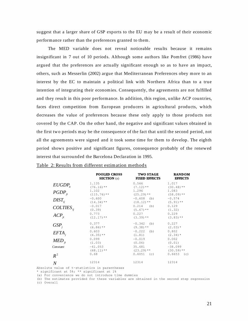
The MED variable does not reveal noticeable results because it remains
insignificant in 7 out of 10 periods. Although some authors like Pomfret (1986) have
argued that the preferences are actually significant enough so as to have an impact,
others, such as Messerlin (2002) argue that Mediterranean Preferences obey more to an
interest by the EC to maintain a political link with Northern Africa than to a true
intention of integrating their economies. Consequently, the agreements are not fulfilled
and they result in this poor performance. In addition, this region, unlike ACP countries,
faces direct competition from European producers in agricultural products, which
decreases the value of preferences because these only apply to those products not
covered by the CAP. On the other hand, the negative and significant values obtained in
the first two periods may be the consequence of the fact that until the second period, not
all the agreements were signed and it took some time for them to develop. The eighth
period shows positive and significant figures, consequence probably of the renewed
interest that surrounded the Barcelona Declaration in 1995.
Table 2: Results from different estimation methods
POOLED CROSS SECTION (a)
TWO STAGEFIXED EFFECTS
RANDOM EFFECTS
itEUGDP 1.135(76.16)**
0.566(7.12)**
1.017(30.48)**
jtPGDP 1.102(115.76)**
1.296(25.29)**
1.083(58.09)**
ijDIST -0.600(14.34)**
-0.608 (b)(18.12)**
-0.574(5.91)**
ijCOLTIES -0.017(0.39)
0.214 (b)(5.67)**
0.129(1.32)
jtACP 0.773(12.17)**
0.227(3.39)**
0.229(3.83)**
jGSP 0.377(6.86)**
-0.342 (b)(9.38)**
0.227(2.03)*
jEFTA 0.603(4.35)**
-0.222 (b)(1.81)
0.802(2.34)*
jtMED 0.099(1.03)
-0.019(0.06)
0.002(0.01)
Constant -41.053(68.11)**
35.481(23.29)**
-38.099(30.59)**
2R 0.68 0.6051 (c) 0.6653 (c)
N 12314 12314 12314
Absolute value of t-statistics in parentheses* significant at 5%; ** significant at 1%(a) For convenience we do not introduce time dummies(b) The estimates provided for these variables are obtained in the second step regression(c) Overall

22
Table 3: Estimation results from different LSDV regressions
(1) (2)
itEUGDP 1.523(7.13)**
1.414(5.81)**
jtPGDP 1.385(18.95)**
1.103(119.99)**
ijDIST -1.706(17.36)**
-0.590(14.50)**
ijCOLTIES 0.188(0.30)
-0.011(0.25)
jtACP 0.127(1.35)
0.770(12.55)**
jGSP 1.956(2.47)*
0.378(7.11)**
jEFTA -0.404(0.45)
0.622(4.64)**
jtMED -0.092(0.22)
0.109(1.17)
2R 0.97 0.96
N 12314 12314
Absolute value of t-statistics in parentheses* significant at 5%; ** significant at 1%(1) LSDV with time, importing and exporting country dummies. (2) LSDV with time and importing country dummies
When analyzing the other methods used, we do find similar results in the different
estimation techniques. GDP and distance remain positive and significant with values
close to one for GDP and between 0.5 and one for distance, in line with the gravity
literature. When analyzing the variables of interest ACP and GSP show lighting figures
following the same pattern in cross-section and panel data, except in the two-stage
regression proposed above, where GSP becomes negative.
Regarding the time dummies of the POLS, periods that show significant numbers
are those in which the accession to the EU of some country took place, with the
exception of period 6. The fact that they are always negative may result from the very
much documented idea that the EU has greatly developed its internal market,
undertaking increasing amounts of trade between its own members. Thus, at each stage
that the EU increased its size, the less need it had to trade with the outside world. At the
same time, the EU market has been constantly seen a progressive removal of internal
barriers to trade so again, less incentive to trade with third countries.
The Hausman test rejects that the unobserved fixed effects are uncorrelated to the
independent variables and thus, we should not rely on the random effects estimates.
However, as Egger and Pfaffermayr (2004) suggest, it is sensible to try this method

23
considering the large sample we handle and we do report the results for comparison
with other models. ACP and GSP show similar results, with ACP and GSP positive and
significant.
The two-stage fixed effect illustrates again a positive and significant impact of
ACP, whereas every other agreement variables show a worse performance being MED
and EFTA insignificant and GSP negative and significant.
The novelty comes now with the sign of the GSP variable. Although further
studies would be needed to assess its causes, there are sufficient arguments to support
the negative sign it takes. The first of such arguments refers to the low utilization that
GSP countries get from their preferences. The utilization rate is defined as the ratio of
products granted GSP over the products covered by the scheme. The trend shown in this
figure is very similar to the one recorded along the history of the GSP. Up to 1994 the
utilization rate was consistently under 35%, according to Sanchez Arnau (2001) and
according to UNCTAD (1999) it went below 30% for LDCs in the period 1994-1997 and
around 50% for non-LDCs in the same period. Comparatively, ACP LDCs utilized 76%
of their preferences in 2001 (UNCTAD, 2003). The reasons behind this low utilization
rate can be found, as suggested by Sapir and Laghammer (1987), in that the EU sets
discretionary quotas or even removes preferences in a given sector to a country when it
just starts to become competitive. In the same line, Borrmann et al (1985) accuse the EU
of tying the granting of GSP preferences to complying with Voluntary Export Restraints
(now decreasing) or with fixed quotas under the Multi Fiber Agreement. In these cases,
the system is flawed from the start. Not least, stringent rules of origin and
administrative complications also make very difficult for exporters to comply with the
necessary requirements (Sanchez Arnau, 2001), at the time of obliging them to raise costs
if they want to attempt exporting under the scheme.
The impact of the Colonial Ties variable is mixed, being significant in only one of
the three methods. Finally, the gravity variables show the expected sign and size, at a
high level of significance.

24
7. CONCLUSIONWe have established the policy framework and the historical background for
EU's trade preferences we have looked into their impact by adding some
econometric improvements to Nilsson’s estimation by undertaking several different
methods of estimation, including three different panel data methods in which we
introduce time-invariant variables.
Although the specification of every model used in this paper may be subject to
improvement, one finding is true: throughout the regressions, ACP preferences have
shown to have a positive impact on trade. Consequently, we have tried to to
reconcile the very discouraging statistics of ACP exports with the econometric
results, providing plausible arguments.
As for GSP, results are mixed and sufficient studies exist justifying both its
success and its failure. More in depth analysis is needed, probably using
disaggregated data and looking into sectorial impact of preferences.
The relevance of the results obtained is important for a number of reasons. The
EU and the ACP countries are currently negotiating the EPAs by which they will
lose a large amount of the preferential treatment. However, it has been foreseen that
those Least Developed Countries belonging to the ACP that are not to join any
regional EPA would automatically fall into the Everything But Arms initiative
(EBA), by which preferential market access is granted at even larger levels than
under Lomé. Countries may then want to think twice about the convenience or not
of joining the EPAs. At the same time, the EU, which has already entered the no-
return point of pursuing the completion of the EPAs and hence, is srtongly
supporting them, should take into account that non-reciprocal market access may
actually help countries promote their exports in a way that is yet to be recognized.
The consequences of realizing this will then be even more important for GSP, that
are not entitled to join the EPAs and will thus remain in their current status quo. Yet,
it must be noted that the GSP scheme is reviewed periodically and is subsequently
renegotiated. Beneficiary countries should be aware of the benefits or costs that it
may bring about to their economies.
The potential for further research stemming from this paper is vast. For instance,
analyzing the effects of the preferential agreements for each of the prospective

25
regional groupings that will form the EPAs will give an idea of who are to lose more
in the new framework. Even more interesting, the study can be done by looking at
what sectors benefited most from preference non-reciprocity. Provided that an FTA
has to cover “substantially all trade” for WTO compliance, there is some scope for
ACP countries to ask non-reciprocity in some sectors where they have proved to
work well.
Finally, a comparison can be made by performing the study the other way
around, this is by looking at the landing market of the ACP and GSP exports, which
would provide evidence to compare between the non-reciprocal trade agreements
signed by the different developed countries.

26
References
Anderson, J. (1979). “A Theoretical Foundation for the Gravity Equation”. The American Economic Review, Vol. 69
Anderson, J. and van Wincoop, E. (2001). “Gravity with Gravitas: A Solution to the Border Puzzle”. NBER Working Paper 8079
Baier, S. L. and Bergstrand, J. H. (2001), “The Growth of World Trade: Tariffs, Transport Costs and Income Similarity”. Journal of International Economics53
Baltagi, B.H., Egger, P. and Pfaffermayr, M. (2003). “A Generalized Design for Bilateral Trade Flow Models”. Economics Letters 80 (2003) 391–397
Bergstrand, J.H. (1985). “The Gravity Equation in International Trade: Some Microeconomic Foundations and Empirical Evidence”. The Review of Economics and Statistics, 67
Bergstrand, J.H. (1989). “The Generalized Gravity Equation, Monopolistic Competition and the Factor-Proportion Theory in International Trade” The Review of Economics and Statistics 71
Borrmann, A. Borrmann, C., Langer, C. and Menck, K-W (1985). “The Significance of the EEC’s Generalized System of Preferences”. Institut für Wirtschaftsforschung
Brenton, P. and F. Di Mauro (1999), “The potential magnitude and impact of FDI flows to CEECs”, Journal of Economic Integration, Vol. 14, n. 1, March, 59-74.
Cheng, I-H. and Wall, H.J. (2004). “Controlling for Heterogeneity Models of Trade and Integration”. Federal Reserve of St. Louis, Working Paper 1999-010E
Cheng, I-H and Tsai, Y-Y (2005), “Estimating the Staged Effects of Regional Economic Integration on Trade Volumes”
Disdier, A-C. and Head, K. (2004), “The Puzzling Persistence of the Distance Effect on Bilateral Trade”, paper formerly titled "Exaggerated Reports of the Death of Distance: Lessons from a Meta-analysis"
DG Development, [EC, 2003] “The new ACP-EU Agreement-General Overview”, European Commission, Brussels, 2003.
DG Trade, [EC, 2001] “Memorandum: EC position in the relation to the development dimension of a new Round of multilateral trade negotiations”, European Commission, Brussels, 2001.
Egger, P. and Pfaffermayr, M. (2004). “Distance, Trade and FDI: A Hausman-Taylor SUR Approach”. Journal of Applied Econometrics, Vol. 19
27
European Commission (2002). “Explanatory Memorandum-Commission Draft Mandate of April 2002”.
Eurostat (2002), “EU-ACP Trade Statistics”, European Commission, Theme 6, 3/2002.
Evenett, Simon J (2002). “The Impact of Economic Sanctions on South African Exports”. Scottish Journal of Political Economy, Vol 49
Feenstra, R.C. (2002). “Border Effects and the Gravity Equation: Consistent Methods of Estimation”. Scottish Journal of Political Economy, Vol 49
Glick, R. and Rose, A.K. (2001). “Does a Currency Union Affect Trade? The Time Series Evidence”. NBER Working Paper No. 8396
Golhar, A.M (1996). “The Generalized System of Preferences and International Flows for the European Community 1971-1991”. California State University, Department of Economics
Haveman, J. and Hummels, D. (2004). “Alternative Hypothesis and the Volume of Trade: The Gravity Equation and the Extent of Specialization”. Canadian Journal of Economics, Vol. 37
Hilberry, R. and Hummels, D. (2003). “International Home-Bias: Some Explanations”. The Review of Economics and Statistics 85
Langhamer, R.J. (1983). Ten Years of the EEC’s Generalized System of Preferences for Developing Countries: Success or Failure?”
Loungani, P., Mody, A. and Razin, A. (2002). “The Global Disconnect: The Role of Transactional Distance and Scale Economies in Gravity Equations”. Scottish Journal of Political Economy, Vol 49
Matyas, L. (1997). “Proper Econometric Specification of the Gravity Model”. The World Economy, Vol 20 (3)
Messerlin, P.A. (2001), “Measuring the Costs of Protection in Europe: European Commercial Policy in the 2000s”, Institute for International Economics, Washington.
Nilsson, L. (2002). “Trading Relations: Is the Road from Lomé to Cotonou Correct?”. Applied Economics, Vol. 34
Onguglu, B. and Ito T. (2003). “How to Make EPAs WTO Compatible? Reforming the Rules on Regional Trade Agreements”. ECDPM Discussion Paper N. 40

28
Ozden C. and Reinhardt E. (2003). “The Perversity of Preferences: The Generalized System of Preferences and Developing Country Trade Policies, 1976-2000”. World Band Policy Research Working Paper 2955
Panagariya, A., (2002). “EU Preferential Trade Policies and Developing Countries”, Available at: http://www.bsos.umd.edu/econ/panagariya/apecon/Policy%20Papers/Mathew-WE.pdf
Pelkmans, J. (2001) “European Integration, methods and economic analysis”, Pearson Education, (2nd ed).
Polak, J.J. (1996). “Is APEC a Natural Trading Region? A Critique of the “Gravity Model” of International Trade”. The World Economy, 19
PriceWaterhouse Coopers (2004). “Sustainability Impact Assessment of the EU-ACP Economic Partnership Agreements-Phase Two”
Rose, A. (2001). “One Money, One Market: Estimating the Effect of Common Currencies to Trade”. NBER, Working Paper 7432
Sapir, A. (1981). “Trade Benefits under the EEC Generalized System of Preferences”
Serlanga, L. and Shin, Y. (2004).”Gravity Models of the Intra-EU Trade: Application of the Hausman-Taylor Estimation in Heterogeneous Panels with Common Time-specific Factors”.
UNCTAD (1999). “Quantifying the Benefits Obtained by Developing Countries from the Generalized System of Preferences”. UNCTAD/ITCD/TSB/Misc.52
Wagner D., Head K. and Ries J. (2002). “Immigration and the Trade of Provinces”. Scottish Journal of Political Economy , Vol 49

29
APPENDIX
Table A1: Selected provisions for ACP countries under the LoméConvention
As Nilsson (2002) describes, apart from almost duty free access to EU
markets, ACP countries enjoy:
Agricultural products not covered by the Common Agricultural Policy
(CAP) enjoy free access to European markets. For those products included
in the CAP there is a restriction on a case-by-case basis.
There are four separate trading protocols on sugar, beef, bananas and
rum§§§§§§§. These protocols allow selected ACP countries to export fixed
quotas of those products to enter EC markets at attractive prices.
STABEX and Sysmin. These are two instruments, which, through EDF
funds, provided funds to ACP countries to compensate for losses on
exports on agricultural products and minerals respectively.
Rules of origin are simpler for ACP countries since input goods coming
from other ACP countries or from the EU are considered as being from the
same country.
§§§§§§§ The rum protocol has not been renewed under the Cotonou Agreement