EUROPEAN UNIVERSITY INSTITUTE DEPARTMENT OF ECONOMICS · EUROPEAN UNIVERSITY INSTITUTE DEPARTMENT...

EUROPEAN UNIVERSITY INSTITUTE DEPARTMENT OF ECONOMICS

EUI Working Paper ECO No. 2005 /5

The Performance of Panel Unit Root

and Stationarity Tests:

Results from a Large Scale Simulation Study

JAROSLAVA HLOUSKOVA

and

MARTIN WAGNER

BADIA FIESOLANA, SAN DOMENICO (FI)

All rights reserved. No part of this paper may be reproduced in any form

Without permission of the author(s).

©2005 Jaroslava Hlouskova and Martin Wagner

Published in Italy in April 2005 European University Institute

Badia Fiesolana I-50016 San Domenico (FI)

Italy

The Performance of Panel Unit Root and Stationarity Tests:

Results from a Large Scale Simulation Study∗

Jaroslava HlouskovaInstitute for Advanced Studies

Department of Economics and Finance

Martin Wagner †

University of BernDepartment of Economics

∗Financial support from the Jubilaumsfonds of the Oesterreichische Nationalbank under grant Nr. 9557is gratefully acknowledged as are the comments of Jorg Breitung, Robert Kunst, Klaus Neusser and PeterPedroni. All remaining errors and shortcomings are entirely ours.

†Part of this work has been done whilst visiting Princeton University and the European University Institute.The hospitality of these institutions is gratefully acknowledged.

1

EUI WP ECO 2005/5

Proposed running head:

Performance of Panel Unit Root and Stationarity Tests

Corresponding author:Martin Wagner

University of BernDepartment of Economics,

Gesellschaftsstrasse 49, CH-3012 Bern, Switzerlandemail: [email protected]

Tel.: ++41 +31 631 47 78Fax: ++41 +31 631 39 92

2

EUI WP ECO 2005/5

Abstract

This paper presents results concerning the size and power of first generation panel unitroot and stationarity tests obtained from a large scale simulation study, with in totalabout 290 million test statistics computed. The tests developed in the following papersare included: Levin, Lin and Chu (2002), Harris and Tzavalis (1999), Breitung (2000),Im, Pesaran and Shin (1997 and 2003), Maddala and Wu (1999), Hadri (2000), and Hadriand Larsson (2005). Our simulation set-up is designed to address i.a. the following issues.First, we assess the performance as a function of the time and the cross-section dimension.Second, we analyze the impact of positive MA roots on the test performance. Third, weinvestigate the power of the panel unit root tests (and the size of the stationarity tests)for a variety of first order autoregressive coefficients. Fourth, we consider both of the twousual specifications of deterministic variables in the unit root literature.

JEL Classification: C12, C15, C23

Keywords: Panel Unit Root Test, Panel Stationarity Test, Size, Power, Simulation Study

3

The Performance of Panel Unit Root and Stationarity Tests

EUI WP ECO 2005/5

1 Introduction

Panel unit root and stationarity tests have become extremely popular and widely used over the

last decade. Given that several such tests are now implemented in commercial software, their

usage will most likely increase further. Thus, it is important to collect evidence on the size

and power of these tests with large-scale simulation studies in order to provide practitioners

with some guidelines for deciding which test to use (for a specific problem or sample size at

hand).

All tests included in this study are so called first generation tests that are designed for

cross-sectionally independent panels. This admittedly very strong assumption simplifies the

derivation of the asymptotic distributions of panel unit root and stationarity tests consider-

ably. We include the panel unit root tests developed in the following papers: Levin, Lin and

Chu (2002), Harris and Tzavalis (1999), Breitung (2000), Im, Pesaran and Shin (1997 and

2003), and Maddala and Wu (1999). We also include two panel stationarity tests, developed

in Hadri (2000), and Hadri and Larsson (2005).

Note that in recent years several tests that avoid the assumption of cross-sectional inde-

pendence have been developed, see e.g. Bai and Ng (2004), Chang (2002), Choi (2002), Moon

and Perron (2004) or Pesaran (2003). These are, however, as of now not widely used and are

also not yet available in commercial software. For these reasons a simulation performance

analysis of these tests is not contained in this paper.

In our simulation study we are primarily interested in the following aspects.1 First, we

investigate the performance of the tests depending upon the time series and cross-sectional

dimension. Since in the derivation of the asymptotic test statistics, different rates of diver-

gence for the time series and the cross-sectional dimension are assumed for different tests

(see Table 1), it is interesting to analyze the performance of the tests when varying the time

and cross-sectional dimensions of the panel. We take for both the time dimension T and

the cross-sectional dimension N all values in the set {10, 15, 20, 25, 50, 100, 200}. Thus, we

investigate in total forty-nine different panel sizes. Second, we assess the performance of the

tests for moving average roots tending to 1. It is well known from the time series unit root

literature (e.g. Agiakloglou and Newbold, 1996) that unit root tests suffer from severe size1Our simulation study is based on ARMA(1,1) processes, respectively on AR(1) processes if the MA co-

efficient is equal to 0, given by (ignoring deterministic components here for brevity): yit = ρyit−1 + uit withuit = εit + cεit−1, where εit ∼ N(0, 1) and are cross-sectionally independent. The parameter c is equal tominus the moving average root.

4

Jaroslava Hlouskova and Martin Wagner

EUI WP ECO 2005/5

distortions for large positive moving average roots. This is clear, since in the case of a mov-

ing average root at 1, the unit root is cancelled and the resultant process is stationary (see

also the discussion in Section 3). In our study we consider moving average roots in the set

{0.2, 0.4, 0.8, 0.9, 0.95, 0.99} and also include the case of no moving average root. This latter

case corresponds in our simulation design to serially uncorrelated errors, which is also the

special case for which some of the tests listed above are developed (e.g. the test of Harris

and Tzavalis, 1999, see the description in Section 2). Third, we study the performance as a

function of the first order autoregressive coefficient ρ. For the power analysis of the panel

unit root tests we take ρ in the set {0.7, 0.8, 0.9, 0.95, 0.99}, and for the size analysis of the

stationarity tests ρ ∈ {0, 0.1, 0.2, 0.3, 0.4, 0.5}. Fourth, we investigate the performance of the

tests for the two most common, and arguably for economic time series most relevant, specifi-

cations of deterministic variables. These are intercepts in the data generating process (DGP)

when stationary but no drifts when integrated (referred to as case 2), and intercepts and

linear trends under stationarity and drifts when integrated (referred to as case 3).2

The number of simulations (i.e. the number of test statistics computed) is given by

290,080,000. This huge number is the product of all parameter choices (for ρ and c) and

sample sizes with the number of replications for each choice, given by 10,000. The total set

of results, comprising about 170 pages of tables and about 30 pages with multiple figures, is

available from the authors upon request.

In Section 3 of the paper we discuss the main observations and display some representative

results graphically. A brief outlook on some of the main findings is: The relative size of the

panel (i.e. the size of T relative to N) has important influence on the performance of the tests.

Especially for T ≤ 50 the performance of all tests is strongly influenced by the cross-sectional

dimension N . For increasingly negative MA coefficients, as expected, size distortions become

more prominent and especially for large negative values of c the size diverges to 1 (even for

T, N → 200). The general impression concerning the size behavior is that the Levin, Lin and

Chu (2002) and Breitung (2000) tests have their size closest to the nominal size. There are,

however, exceptions (see the discussion in Section 3). Concerning power we observe that for

case 2 either the Levin, Lin and Chu (2002) test or the Breitung (2000) test have the highest

power, whereas in case 3 there exist parameter constellations and sample sizes such that each2A further issue that is studied is the effect of the choice of the autoregressive lag lengths, as explained in

Section 2, on the performance of the tests.

5


EUI WP ECO 2005/5

of the considered tests has highest power.

The stationarity tests show very poor performance. The tests essentially reject the null

hypothesis of stationarity for all processes that are not ‘close to white noise’, for all but

the smallest values of T . This finding is not inconsistent with the fact that empirical studies

usually reject the null hypothesis of stationarity when using the tests of Hadri (2000) or Hadri

and Larsson (2005).

The paper is organized as follows: Section 2 describes the implemented panel unit root

and stationarity tests. Section 3 presents the simulation set-up and discusses the simulation

results and Section 4 draws some conclusions. An appendix containing additional figures

follows the main text.

2 The Panel Unit Root and Stationarity Tests

In this section we describe the implemented panel unit root and stationarity tests. We include

a relatively detailed description here for two reasons. First, the detailed description allows

the reader to see the differences and similarities across tests clearly at one place. Second,

our description is intended to be detailed enough to allow the reader to implement the tests

herself.

The data generating process (DGP) for which the considered tests are designed is in its

most general form given by

yit = αi + βit + ρiyit−1 + uit, i = 1, . . . , N and t = 1, . . . , T (1)

where αi, βi ∈ R and −1 < ρi ≤ 1.3 The noise processes uit are stationary ARMA processes,

i.e. the stationary solutions to ai(z)uit = bi(z)εit, ai(z) = 1 + ai,1z + · · · + ai,pizpi , ai,pi �= 0,

bi(z) = 1 + bi,1z + · · · + bi,qizqi , bi,qi �= 0, ai(z) �= 0 for all |z| ≤ 1, bi(z) �= 0 for all |z| ≤ 1 and

with ai(z) and bi(z) relative prime. The innovation sequences εit are i.i.d. with variances σ2i

and finite fourth moments and are assumed to be cross-sectionally independent.

The above assumptions on the noise processes are stronger than required for the applica-

bility of functional limit theorems. In particular the assumptions guarantee a finite long-run

variance of the processes uit, i.e. a bounded spectrum of uit at frequency 0. The long-run3In all our simulations we restrict attention to balanced panels, i.e. to panels where the number of obser-

vations is identical for all cross-sectional units. This is of course not required for all tests investigated. Somecross-sectional dependence can be handled with the tests discussed by including (random) time effects. We donot discuss this issue here.

6


EUI WP ECO 2005/5

variance of uit is given by 2π times the spectrum of uit at frequency 0. For stationary ARMA

processes the long-run variance, σ2ui,LR say, is immediately found to be σ2

i b2i (1)/a2

i (1).4

Some of the tests discussed below are designed for more restricted DGPs than the gen-

eral DGP given in (1). In particular some tests are restricted to serially uncorrelated noise

processes uit.

As in the time series unit root literature, three specifications for the deterministic compo-

nents are considered in the panel unit root literature. These are DGPs with no deterministic

component (d1t = {�}), DGPs with intercept only (d2t = {1}) and DGPs containing both

intercept and linear trend (d3t = {1, t}). Exactly as in the time series literature, three cases

concerning the deterministic variables in the presence of a unit root and under stationarity

are considered most relevant. Case 1 contains no deterministic components in both the sta-

tionary and the nonstationary case, case 2 allows for intercepts in the DGP when stationary

but excludes a drift when integrated, and case 3 allows for intercepts and linear trends under

stationarity and for a drift when a unit root is present.

2.1 Panel Unit Root Tests

Levin, Lin (and Chu): We start the description of the unit root tests with the Levin and Lin

(1993) tests, abbreviated by LL93 henceforth. Their results have only been recently published

in Levin, Lin and Chu (2002).5 The null hypothesis of the LL93 test is H0 : ρi = 1 for i =

1, . . . , N , against the homogenous alternative H11 : −1 < ρi = ρ < 1 for i = 1, . . . , N . Thus,

under the homogenous alternative the first order serial correlation coefficient ρ is required to

be identical in all units. This restriction stems from the fact that the test statistic is computed

in a pooled fashion.

The approach is most easily described as a three-step procedure, with preliminary regres-

sions and normalizations necessitated by cross-sectional heterogeneity. In the first step for4Solving the ARMA equation for the Wold representation uit = ci(z)εt =

∑∞j=0 cijεt−j , the (short-run)

variance of uit is given by σ2ui = σ2

i

∑∞j=0 c2

ij and the long-run variance is given by σ2ui,LR = σ2

i (∑∞

j=0 cij)2.

5Important foundations have already been laid in Levin and Lin (1992), where panel unit root tests havebeen developed for homogenous panels. These are panels where loosely speaking the ARMA coefficients areidentical for all uit.

7


EUI WP ECO 2005/5

each individual series an ADF type regression of the form6

∆yit = (ρi − 1)yit−1 +pi∑

j=1

γij∆yit−j + δmidmt + vit, m = 1, 2, 3 (2)

is performed, where vit denotes the residual process of the AR equation. If the processes are

AR processes and the AR orders pi are specified correctly, then vit = uit holds. Here and

throughout the paper m indexes the case considered. The lag lengths in the autoregressive

test equations have to be increased appropriately as a function of the time dimension of the

panel to ensure consistency, if the processes uit are indeed ARMA processes. More specifically

pi(T ) ∼ T κ, with 0 < κ ≤ 1/4 has to be assumed in the ARMA case. In practical applications

some significance testing on the estimated γij , an information criterion or checking for no serial

correlation in the estimated residuals vit is used to determine the lag lengths pi. Then, for

given pi, orthogonalized residuals are obtained from two auxiliary regressions. eit say, from

a regression of ∆yit on the lagged differences ∆yit−j , j = 1, . . . , pi and dmt, and fit−1 say,

from a regression of yit−1 on the same set of regressors. These residuals are standardized by

the regression standard error from regressing eit on fit−1, σvi say, to obtain the standardized

residuals eit, fit−1.

The second step is to obtain an estimate of the ratio of the long-run variance to the

short-run variance of ∆yit, or equivalently of uit. The definition of the long-run variance,

σ2ui,LR = σ2

ui + 2∑∞

j=1 E(uitui,t−j) immediately leads to an estimator of the form

σ2ui,LR =

1T

T∑t=1

u2it +

2T

L∑j=1

w(j, L)T∑

t=j+1

uitui,t−j (3)

where the lag truncation parameter L can be chosen e.g. according to Andrews (1991) or

Newey and West (1994). In the above equation we choose as estimate for the unobserved

noise uit = ∆yit − δmidmt.7 In our simulations the weights are given by w(j, L) = 1 − jL+1 .

This kernel is known as Bartlett kernel. The estimated individual specific ratio of long-

run to short-run variance is defined as s2i = σ2

ui,LR/σ2ui, with σ2

ui = 1T

∑Tt=1 u2

it. Denote by

6Actually, it is recommended by Levin, Lin and Chu (2002), that in a first step the cross-section averageyt = 1

N

∑Ni=1 yit is removed from the observations. This stems from the fact that the presence of time specific

aggregate effects does not change the asymptotic properties, when the tests are performed on the transformedvariables yit − yt. Thus, as indicated already, a limited amount of dependence across the errors is allowed for,in a form that can easily be removed. For the panels we simulate this step is not required.

7Note that a direct estimate for the long-run variance is given by σ2vi(1−

∑pij=1 γij)

−2. Levin, Lin and Chu(2002) indicate that variance estimation based on the first differences is found to have a smaller bias under thenull hypothesis, which in turn should help to improve both (finite sample) size and power of the panel unitroot test.

8


EUI WP ECO 2005/5

SNT = 1/N∑N

i=1 si. The quantity SNT is used later for the construction of correction factors

to adjust the t-statistics of the hypothesis that φi := (ρi − 1) = 0 for i = 1, . . . , N .

The test statistic itself, which can be based on either the coefficient φ or on the corre-

sponding t-statistic, is computed from the pooled regression of eit on fit−1,

φ =

∑Ni=1

∑Tt=pi+2 eitfit−1∑N

i=1

∑Tt=pi+2 f2

it−1

(4)

The null hypothesis is H0 : φ = 0, and the test we use in the simulations is based on

the corresponding t-statistic, tφ say. The standard deviation of φ can be straightforwardly

computed from the pooled regression (4), since due to the pre-filtering all the errors in this

pooled regression have the same (asymptotic) variance.

For case 1 and test LL931, Levin and Lin (1993) show that tφ ⇒ N(0, 1). For cases 2

and 3 and tests LL932 and LL933, the t-statistic tφ diverges to minus infinity, and thus

has to be re-centered and normalized to induce convergence towards a well defined limiting

distribution,

t∗φ =tφ − NT SNT STD(φ)µmT

σmT(5)

Here µmT and σmT denote mean and variance correction factors, tabulated for various panel

dimensions in Table 2 on page 14 of Levin, Lin and Chu (2002). T denotes the average

effective sample size across the individual units and STD(φ) denotes the standard deviation

of φ. The adjusted t-statistics t∗φ converge to the standard normal distribution for cases 2

and 3.

As a remark note that the relative rates of divergence for N and T required for the

consistency proofs of the test statistics differ between case 1 and cases 2 and 3. For case 1,

limN,T

√N/T → 0 is required and for cases 2 and 3 limN,T N/T → 0 is imposed. For a

detailed discussion of the relevant limit concepts for nonstationary panels and the relations

among the different limit concepts see Phillips and Moon (1999).

Harris and Tzavalis: The test of Harris and Tzavalis (1999), labelled HT , augments

the analysis of Levin and Lin (1993) by considering inference for fixed T and asymptotics only

in the cross-section dimension N . They obtain their results (closed form correction factors

as a function of T ), however, only for serially uncorrelated errors. All three cases for the

deterministic variables are considered. For fixed T , the authors derive asymptotic normality

(for N → ∞) of the appropriately normalized and centered coefficients φ (which are for cases 2

9


EUI WP ECO 2005/5

and 3 inconsistent for T → ∞, as can be seen from the above discussion). In particular the

following results are shown:

√N(ρ − 1 − Bm) ⇒ N(0, Cm) (6)

with B1 = 0, C1 = 2/T (T − 1), B2 = −3/(T + 1), C2 = 3(17T 2 − 20T + 17)/5(T − 1)(T + 1)3

and B3 = −7.5/(T + 2) and C3 = 15(193T 2 − 728T + 1147)/112(T − 2)(T + 2)3.

The practical relevance of this result is to obtain improved tests for panels with small T

and large N . E.g. for case 1 the variance scaling factor used for testing is – when the limit is

taken only with respect to N – by a factor T/(T − 1) smaller than the LL93 scaling factor.

This implies immediately that, compared to the fixed-T test, the LL93 test will be oversized,

i.e. the test based on test statistics constructed by letting both T and N tend to infinity will

reject the null hypothesis more often. The drawback of the Harris and Tzavalis results is the

mentioned restriction to white noise errors.

Breitung: Breitung (2000) develops a pooled panel unit root test that does not require

bias correction factors, which is achieved by appropriate (depending upon case considered)

variable transformations. Due to its pooled construction also the Breitung test, UB hence-

forth, is a test against the homogenous alternative.

Case 1 is exactly similar to the Levin, Lin and Chu (2002) test, since in this case no bias

corrections are required. For case 2 bias correction factors are avoided by subtracting the

initial observation.8 Thus, case 2 is equal to case 1 of LL93 on the transformed variables

yit = yit − yit−1. In both cases the asymptotic distribution of the test statistic is standard

normal without the need of resorting to correction factors.

For case 3 slightly more complicated correction factors have to be applied, after serial

correlation has been removed with first step regressions. There are two ways of removing the

serial correlation, the first is resorting to preliminary regressions as in the description of the

Levin, Lin and Chu (2002) test and the second, suggested by Breitung and Das (2005) to

have better small sample performance, is pre-whitening. Pre-whitening involves in the first

step the following regressions (for each i)

∆yit = αi +pi∑

j=1

γij∆yit−j + vit, (7)

8Subtracting the initial observation instead of the mean circumvents the Nickell bias.

10


EUI WP ECO 2005/5

from which the residuals eit and fit are computed as follows

eit = ∆yit −pi∑

j=1

γij∆yit−j , (8)

fit−1 = yit−1 −pi∑

j=1

γijyit−j−1 (9)

The residuals are then standardized by the regression standard error of (7) to obtain eit and

fit−1. Here we use for simplicity the same notation as for the residuals obtained via auxiliary

regressions. We do this for notational simplicity and also because the two approaches are

asymptotically equivalent. Finally the residuals eit and fit are orthogonalized as follows:

e∗it =

√T − t

T − t + 1

(∆eit − 1

T − t(∆eit+1 + · · · + ∆eiT )

)(10)

f∗it = fit−1 − fi1 +

t − 1T

(fiT − fi1) (11)

Here we denote for notational simplicity by T also the sample size after the auxiliary regres-

sions. Now the unit root test is performed in the pooled regression

e∗it = φ∗f∗it + v∗it (12)

by testing the hypothesis H0 : φ∗ = 0. Breitung shows that the t-statistic of this test has

a standard Normal limiting distribution (for a sequential limit of first T → ∞ followed by

N → ∞).

We now turn to panel unit root tests that are designed against the heterogeneous alter-

native H21 : −1 < ρi < 1 for i = 1, . . . , N1 and ρi = 1 for i = N1, . . . , N . For asymptotic

consistency (in N) of these tests, a non-vanishing fraction of the individual units has to be

stationary under the alternative, i.e. limN→∞ N1/N > 0. The tests are based on group-mean

estimation and test statistics, i.e. on appropriately combined individual time series unit root

tests.

Im, Pesaran and Shin: In two papers Im, Pesaran and Shin (1997 and 2003), hence-

forth abbreviated as IPS, present two group-mean panel unit root tests designed against the

11


EUI WP ECO 2005/5

heterogeneous alternative. IPS consider only cases 2 and 3 and allow for individual specific

autoregressive structures and individual specific variances.9

Note that in order to apply the tables with correction factors provided by Im, Pesaran and

Shin, identical autoregressive lag lengths for all units and a balanced panel are required. The

two tests are given by a t-test based on ADF regressions (IPSt) and a Lagrange multiplier

(LM) test (IPSLM ).

For the case of serially uncorrelated errors, the test statistics are derived for fixed T and

asymptotic N . However, in that case the t-test is not exactly a ‘usual t-test’, since the applied

variance estimator is taken from the restricted regression where the coefficient on the lagged

level term is set equal to 0. IPS establish asymptotic normality (for N → ∞) for case 2 when

T > 5 and for case 3 when T > 6.

For serially correlated errors sequential limit theory is applied, with T → ∞ followed by

N → ∞, with a particular relative rate restriction for the LM test, with limN/T = k for

some k > 0.

We now describe the construction of the t-test for serially correlated errors. For the

moment we focus on only one unit i. The errors uit are assumed to follow an AR(pi + 1)

process. Thus, the t-test statistic from the ADF regression (2) can be written as follows, with

m = 2, 3 indicating again the deterministic terms present in the regression:

tiT,m(pi, γi) =

√T − pi − m(y′

i,−1MQi∆yi)

(y′i,−1MQiyi,−1)1/2(∆y′

iMXi∆yi)1/2, m = 2, 3 (13)

using the notation γi = (γi1, . . . , γipi)′, yi,−1 = [yi0, . . . , yiT−1]

′, ∆yi,−s = [∆yi1−s, . . . ,∆yiT−s]′,

s = 0, . . . , pi, ∆yi = ∆yi,−0, d2T = [1, . . . , 1]′, t = [1, . . . , T ]′, d3T = [d2T , t], Qi =

[dmT , ∆yi,−1, . . . ,∆yi,−pi ], MQi = IT − Qi(Q′iQi)−1Qi, Xi = [yi,−1,Qi], MXi = IT −

Xi(X′iXi)−1Xi (suppressing the index m in the matrix notation for Qi and Xi). For fi-

nite values of T , the statistics tiT,m depend upon the nuisance parameters γi. IPS show that

this dependence vanishes for T → ∞, but that the bias of the individual t-statistics under the

null remains. This follows from the fact that under the null hypothesis convergence to the

Dickey-Fuller distribution corresponding to the model prevails. Therefore mean and variance

correction factors have to be introduced. The proposed test statistic itself is the cross-section9The same arguments as used in Levin and Lin (1993) might cover the case of ARMA disturbances, with

the lag lengths in autoregressive approximations increasing with the sample size at an appropriate rate. Im,Pesaran and Shin seem to share this view given that one of the reported simulation experiments is based onmoving average dynamics for the errors.

12


EUI WP ECO 2005/5

average of the corrected t-statistics:

IPSt,m(p, γ) =

√N{tm − 1

N

∑Ni=1 E(tiT,m(pi,0)|ρi = 1)}√

1N

∑Ni=1 V ar(tiT,m(pi,0)|ρi = 1)

⇒ N(0, 1) (14)

where tm = 1N

∑Ni=1 tiT,m(pi, γi), p = [p1, . . . , pN ]′ and γ = [γ′

1, . . . , γ′N ]′. The correction

factors E(tiT,m(pi,0)|ρi = 1) and V ar(tiT,m(pi,0)|ρi = 1) are simulated for m = 2, 3 for a

set of values for T and lag lengths p (see Table 3 in Im, Pesaran and Shin, 2003). Thus,

without resorting to further tailor made Monte Carlo simulations, the applicability of the IPS

tests is limited to balanced panels and identical lag lengths in all individual equations (and

error processes). Simulating the mean and variance only as a function of the lag and setting

the nuisance parameters γi = 0 introduces a bias of order Op(1/√

T ), but still takes into

account the finite sample effect of the different lag lengths chosen.10 Note that for T → ∞the t-statistics converge to the Dickey-Fuller distributions and thus the asymptotic correction

factors are the mean and variance of the Dickey-Fuller statistic corresponding to the model.

Thus, if one wants to avoid using simulated critical values one can also refer to the asymptotic

values for T → ∞ (which has the additional advantage of allowing the use of cross-section

specific lag lengths pi).

Let us now turn to the Lagrange multiplier test. Using the Lagrange multiplier test

principle implies that the alternative is actually given by ρi �= 1 as opposed to ρi < 1, although

the authors propose to use a 1-sided test nevertheless (see Im, Pesaran and Shin, 1997,

Remark 3.2). For each individual unit the test statistic is given by

LMiT,m(pi, γi) = T(∆y′

iMQiyi,−1)(y′i,−1MQiyi,−1)−1(y′

i,−1MQi∆yi)(y′

i,−1MQiyi,−1)(15)

As for the t-test, for T → ∞ the dependence upon nuisance parameters disappears. Paralleling

the above argument the Lagrange multiplier panel unit root test statistic is given by

IPSLM,m(p, γ) =√

N{LMm− 1N

∑Ni=1 E(LMiT,m(pi,0)|ρi=1)}√

1N

∑Ni=1 V ar(LMiT,m(pi,0)|ρi=1)

⇒ N(0, 1)(16)

where LMm = 1N

∑Ni=1 LMiT,m. As indicated above, this result is developed for limN/T = k.

The correction factors are available in Im, Pesaran and Shin (1997).10Simulation of these values for different values of T and p proceeds by generating ∆yt = εt, with εt i.i.d.

N(0, 1) for t = 1, . . . , T and computing the t-statistic for ρ = 1 in the ADF regression (2) for j = p where dmt

is included.

13


EUI WP ECO 2005/5

Maddala and Wu: Maddala and Wu (1999) tackle the panel unit root testing problem

with a very elegant idea dating back to Fisher (1932).11 The basic idea of Fisher can be

explained with the following simple observations that hold for any testing problem with con-

tinuous test statistics: First, under the null-hypothesis the p-values, π say, of the test statistic

are uniformly distributed on the interval [0, 1]. Second, −2 log π is therefore distributed as

χ22, with log denoting the natural logarithm. Third, for a set of independent test statistics

−2∑N

i=1 log πi is consequently distributed as χ22N under the null hypothesis.

These basic observations can be very fruitfully applied to the panel unit root testing

problem, provided that cross-sectional independence is assumed. Any unit root test with

continuous test statistic performed on the individual units can be used to construct a Fisher

type panel unit root test, provided that the p-values are available or can be simulated. We

implement this idea by applying ADF tests on the individual units. For ADF tests estimated

p-values for cases 1 to 3 can be obtained due to the extensive simulation work of James

MacKinnon and his coauthors (see for one example MacKinnon, 1994). Note as a further

advantage that the Fisher test neither requires a balanced panel nor identical lag lengths in

the individual equations. We have implemented the test for cases 1 to 3 based on individual

ADF tests, they are labelled as MWm for m = 1, 2, 3 (ignoring the dependence upon ADF in

the notation).

2.2 Panel Stationarity Tests

Hadri: Hadri (2000) proposes a panel extension of the Kwiatkowski et al. (1992) test, labelled

HLM henceforth. Cases 2 and 3 are considered. The null hypothesis is stationarity in all

units against the alternative of a unit root in all units. The alternative of a unit root in

all cross-sectional units stems from the fact that this test is based on pooling. Individual

specific variances and correlation patterns are allowed for. We start our discussion of the test

statistics, however, assuming for the moment serially uncorrelated errors and only allow for

individual specific variances σ2i .

The test is constructed as a residual based Lagrange multiplier test with the residuals

taken from the regressions

yit = δmidmt + εit, m = 2, 3 (17)11Choi (2001) presents very similar tests that only differ in the scaling in order to obtain asymptotic normality

for N → ∞.

14


EUI WP ECO 2005/5

for i = 1, . . . , N . Denote the residuals of regression (17) by eit, and their partial sum by

Sit =∑t

j=1 eij . The test statistic is then given by (m indexing again the case investigated)

HLM,m =1

NT 2

N∑i=1

T∑t=1

S2it

σ2ei

(18)

with σ2ei = 1/T

∑Tt=1 e2

it.

Expression (18) can be disentangled to highlight the principle of the test. Under the null

hypothesis of stationarity, the expressions in the numerator of the test statistics, 1/T 2∑T

t=1 S2it

(for any fixed i) converge for T → ∞ to an integral of a Brownian motion of the form

σ2ei

∫V 2

m(r)dr. This follows from the fact that this term is the appropriately scaled sum of

squared partial sums of εit. The denominator scales the expression by the variance (see e.g.

Phillips, 1987). For m = 2 it holds that V2(r) = W (r) − rW (1) (the so called Brownian

bridge) and for m = 3, V3(r) is the so called second level Brownian bridge.12 Recentering and

rescaling the expressions by subtracting their mean and dividing by their standard deviation

gives rise to asymptotic standard normality in the sequential limit (with now N → ∞)

ZLM,m =

√N(HLM,m − ξm)

ζm⇒ N(0, 1) (19)

Due to the simple shape of the correction terms, closed form solutions for the correction

factors can be easily obtained. They are given by ξ2 = 1/6, ζ2 =√

1/45 and ξ3 = 1/15, ζ3 =√11/6300. The extension to serially correlated errors is straightforward, the variance estima-

tor σ2ei only has to be replaced by an estimator of the long-run variance of the noise processes

in (17).

Hadri and Larsson: Hadri and Larsson (2005) extend the analysis of Hadri (2000) by

considering the statistics for fixed T (the test is therefore abbreviated by HT ). The key

ingredient for their result is the derivation of the exact finite sample mean and variance of

the Kwiatkowski et al. (1992) test statistic that forms the individual unit building block for

the Hadri type test statistic. For cases 2 and 3 they compute the exact mean and variance

of ηiTm = 1/T 2∑T

t=1 S2iT /σ2

ei, which is the core expression of the Hadri type test statistics,

compare (18). Standard asymptotic theory for N then delivers asymptotic normality

HT,m =1√N

N∑i=1

(ηiTm − EηiTm√

V ar(ηiTm)

)⇒ N(0, 1) (20)

12These are, of course, the well known limits known from the time series unit root literature. We haveencountered related expressions already in the discussions of the Levin, Lin and Chu (2002) and the Im,Pesaran and Shin (2003) tests.

15


EUI WP ECO 2005/5

with EηiT2 = (T +1)/6T , V arηiT2 = (T 2+1)/20T 2−((T +1)/6T )2 and EηiT3 = (T +2)/15T ,

V arηiT3 = (T + 2)(13T + 23)/2100T 3 − ((T + 2)/15T )2.

The potential advantage of these finite T statistics is, as noted above in the discussion of

the Harris and Tzavalis (1999) test, to avoid oversized tests due to treating not only N but

also T asymptotic.

Note finally that serial correlation can be handled again by appropriately computing the

individual specific long-run variances as discussed several times in this section. Since for

fixed T only estimates for the long-run variances are available it is not clear that the above

result (20) holds exactly (for finite T and N → ∞).

3 The Simulation Study

In this section we present a representative selection of results obtained from our large scale

simulation study. Due to space constraints we only report a small subset of results and focus

on some of the main observations that emerge. The full set of results (containing about 170

pages of tables and about 30 pages with multiple figures) is available from the authors upon

request.

We only report results for cases 2 and 3, since case 1 is of hardly any empirical relevance

for economic time series. The computations have been performed in GAUSS.13 The number

of replications is 10,000 for each DGP and sample size. Both the time dimension T and the

cross-sectional dimension N assume all values in the set {10, 15, 20, 25, 50, 100, 200}. Thus,

we consider in total forty-nine different panel sizes. The performance of the tests in relation

to the sample dimensions T and N is one aspect of interest in our simulations. Remember

from the discussion in the previous section that the tests rely upon different divergence rates

for T and N , summarized for convenience in Table 1. One question in this respect is whether

the finite-T tests of Harris and Tzavalis (1999) and Hadri and Larsson (2005) exhibit less size

distortions than their asymptotic-T counterparts for panels with T small (compared to N).

The DGPs simulated for case 2 are of the following form

yit = αi(1 − ρ) + ρyit−1 + uit

uit = εit + cεit−1(21)

with εit ∼ N(0, 1). The parameters chosen in the simulations are α = [α1, . . . , αN ], ρ

and c. We summarize the dependency of the DGP upon these parameters notationally as13The computations have been performed with a substantially extended, corrected and modified set of

routines based originally on Chiang and Kao (2002). A description of major changes is available upon request.

16


EUI WP ECO 2005/5

The Asymptotics Used in the Derivation of the Test StatisticsLL93 N → ∞ following T → ∞, N/T → 0 (for cases 2 and 3)

HT N → ∞ and T fixUB N → ∞ following T → ∞

IPS White Noise: N → ∞ and T fixSerial Correlation: N → ∞ following T → ∞, N/T → k > 0

MW N , T fix, approximation of ADF p-values for finite T

HLM N → ∞ following T → ∞HT N → ∞ and T fix

Table 1: Summary of asymptotic behavior required T and N for the derivation of the limitingdistribution of the tests.

DGP2(α, ρ, c). Note for completeness that the formulation of the intercepts as αi(1 − ρ) en-

sures that in the unit root case (when ρ = 1) no drift appears. Consequently, when ρ = 1

we set α = 0 in the simulations for computational efficiency. Otherwise, the coefficients αi

are chosen uniformly distributed over the interval 0 to 4, i.e. αi ∼ U [0, 4]. We parameterize

case 3, DGP3(α, ρ, c), as

yit = αi + αi(1 − ρ)t + ρyit−1 + uit

uit = εit + cεit−1(22)

with εit ∼ N(0, 1). This formulation allows for a linear trend in the absence of a unit root

and for a drift in the presence of a unit root. The coefficients αi are, as for case 2, U [0, 4]

distributed.

For the unit root tests the following values are chosen for ρ: 0.7, 0.8, 0.9, 0.95, 0.99 and

1.14 The former five values are used to assess the power of the tests against the stationary

alternative. For the stationarity tests we only report results for ρ ∈ {0, 0.1, 0.2, 0.3, 0.4, 0.5}for the size analysis. These values are chosen because preliminary simulations have shown

that the stationarity tests fail to deliver acceptable results for larger values, i.e. for ρ ∈{0.6, 0.7, 0.8, 0.9, 0.95, 0.99}.

For the moving average parameter c we choose all values in the set {0,−0.2,−0.4,−0.8,

−0.9,−0.95,−0.99} for the size study of the panel unit root tests and the power study of

the stationarity tests, and c ∈ {0,−0.2,−0.4} for the power study of the panel unit root

tests and the size study of the stationarity tests. Why do we choose 0 and negative values14Preliminary simulations have shown that for values of ρ up to 0.6 all tests exhibit satisfactory power

behavior already for medium sized panels. We thus focus here only on those cases for ρ, where differentialresults across tests can be observed widely across the simulation experiments. The case ρ = 0 is included asbenchmark case. Also the case ρ = 0 is the single case for which the tests designed for serially uncorrelatedcan be applied with all assumptions fulfilled.

17


EUI WP ECO 2005/5

approaching -1? It is well known from the time series unit root literature that unit root tests

suffer from severe size distortions in the presence of large positive MA roots. In the boundary

case with the MA coefficient equal to -1, the unit root is cancelled and the resultant process

is stationary. Thus, the closer the coefficient c is to -1, the larger the size distortions are

expected to be for any given sample size.15 With our set-up we can analyze the extent of

the size distortions as a function of both N and T . The value c = 0 serves as a benchmark

case with no serial correlation and is also the special case for which the test of Harris and

Tzavalis (1999) is designed for. For c �= 0, the choice of the lag lengths in the autoregressive

approximations that most of the tests are based on becomes potentially important. We try

to assess the importance of this choice by running the panel unit root tests (in case of MA

errors) for several choices for the autoregressive lag length. One of our choices is BIC. We,

however, also compute the test statistics for c �= 0 for autoregressive lag lengths varying from

0 to 2 (since 2 is for all values of c ≥ −0.4 the maximum lag length according to BIC), to assess

the influence of the lag length selection on the size behavior (see the discussion below on the

effect of lag length selection).16 Note that we choose the value of c identical for all cross-

section members. We do this to ‘cleanly’ study the effect of the moving average coefficient

approaching -1, which is harder to assess when the MA coefficients are drawn randomly for

the cross-section units.

The careful reader will have observed that our simulated DGPs all have a cross-sectionally

identical coefficient ρ under both the null and the alternative. Thus, we are in effect in a

situation where we generate data either under the null hypothesis or under the homogenous

alternative. We do this, because only the more restrictive homogenous alternative can be

used for all tests described in the previous section. This implies to a certain extent that

we do not explore the additional degree of freedom that the tests against the heterogeneous

alternative (IPS and MW) possess. Thus, to a certain extent the pooled tests are favored in our

comparison, since the last step regression to estimate ρ, is for these tests one pooled regression

with about N(T−p) observations, and consists of N regressions with T−p observations for the

group-mean tests (denoting with p the autoregressive lag length). An analysis of group-mean15It is straightforward to show that the asymptotic bias for T → ∞ of ρ, estimated from an AR(1) equation

when the errors are not white noise but MA(1), is linear in the MA coefficient c. This holds both in thestationary and the integrated case.

16Some (unreported) simulation results also suggest that choosing lag lengths by starting with a large initialnumber of lags and sequential truncation of one lag until the coefficient to the largest lag is significant canimprove performance sometimes. However, we do not have systematic evidence on the effects of lag lengthselection on the test performance (for different sample sizes).

18


EUI WP ECO 2005/5

tests and their performance under the heterogeneous alternative is not considered separately

in this paper. The relative ranking of the group mean tests in our simulations, may however

still serve as an indicator for the relative performance of these tests.17

3.1 The Size of the Panel Unit Root Tests

In this subsection we report the results of the analysis of the actual size of the panel unit root

tests.18 The nominal critical level in the simulation study is 5%. As noted above, the Harris

and Tzavalis (1999) test is only designed for serially uncorrelated errors. Thus, this test is

only computed for c = 0. All other tests (LL93, UB, IPSt, IPSLM and MW ) are computed

for all values of c.

We start with case 2 in Figures 1 and 2 and Figures 3 and 4 display results for case 3.

For these and all other figures, it is always the cross-sectional dimension N that varies along

the horizontal axis.19

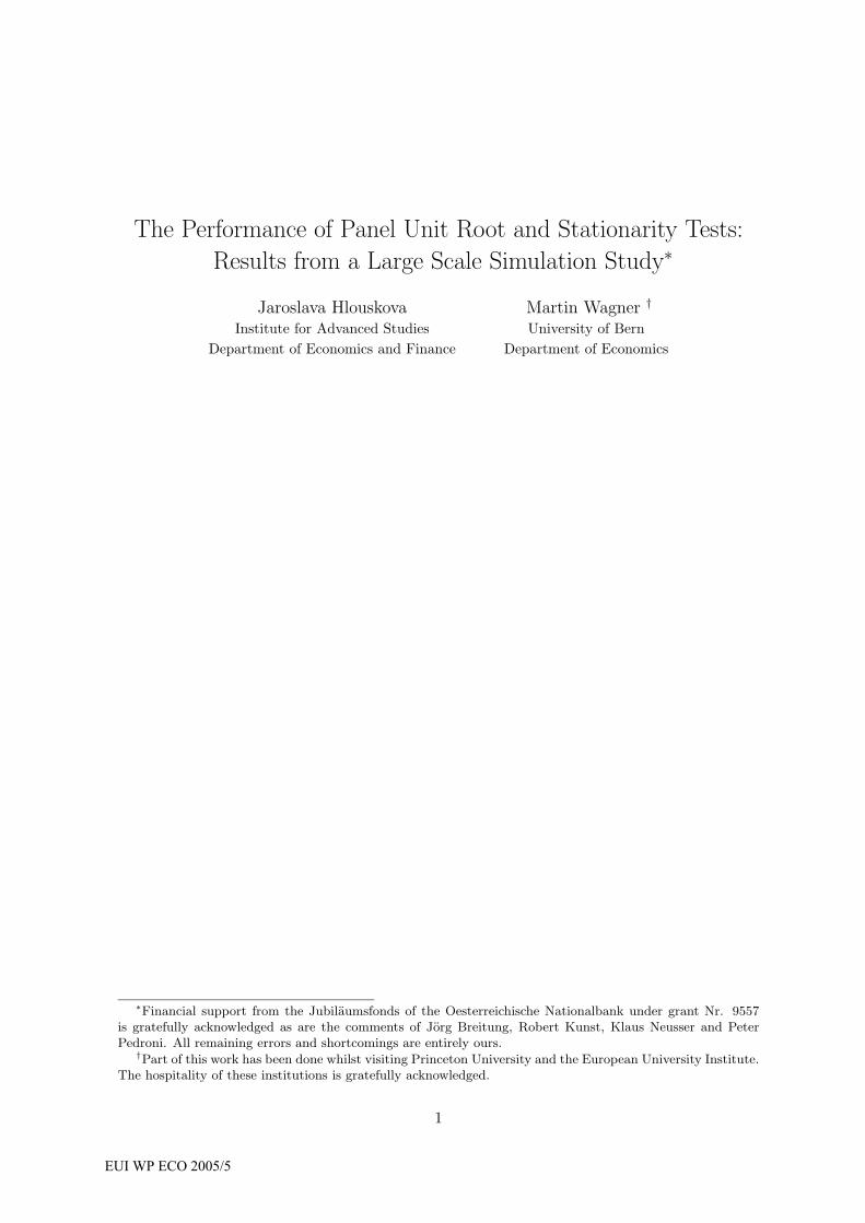
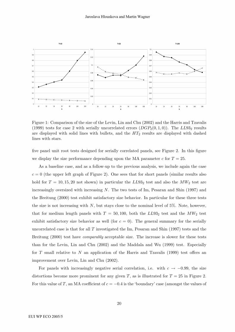
Figure 1 displays for c = 0 a comparison of the size of the LL932 test and the HT2

test, which is – as has been discussed – a fixed T version of the LL932 test (for serially

uncorrelated errors). The graphs display the size for all values of N for T ∈ {10, 25, 100}.It becomes clearly visible that for small T like 10, the Harris and Tzavalis (1999) test has

superior size performance. The difference in size performance increases with N , for both

T = 10 and T = 25 (in the latter case for N ≥ 25). This, of course, can be traced back to the

fact that the asymptotic normality and the corresponding critical values of the LL932 test

are based on sequential limit theory with N → ∞ following T → ∞ and furthermore with

lim N/T → 0, see Table 1. For larger T , the improved performance of the ADF-type unit

root of the LL932 test kicks in and starts to outweigh the performance deterioration with

increasing N . For T = 100 the size of LL932 is monotonically decreasing towards 5% in the

right graph of Figure 1.

Thus, for panels with little or no serial correlation the HT test can be considered an

interesting extension or implementation of the LL93 test. No serial error correlation is unfor-

tunately a rare case for economic time series. We therefore turn next to study the size of the17Karlsson and Lothgren (2000) present some simulation results in this respect.18In this study we use the word size simply to denote the type I error rate at the actual DGP. This is not the

size as defined by the maximal type I error rate over all feasible DGPs under the null hypothesis, see Horowitzand Savin (2000) for an excellent discussion of this issue.

19Please note that the vertical axis is not scaled identically across the sub-plots of the figures. This stemsfrom the fact that for all the experiments we display, identical vertical scaling leads to closely bundled lines insome of the figures.

19


EUI WP ECO 2005/5

T=10

0

0.1

0.2

0.3

0.4

0.5

0.6

0.7

0.8

0.9

1

10 15 20 25 50 100 200

N

T=25

0

0.02

0.04

0.06

0.08

0.1

0.12

0.14

10 15 20 25 50 100 200

N

T=100

0

0.01

0.02

0.03

0.04

0.05

0.06

0.07

0.08

0.09

0.1

10 15 20 25 50 100 200

N

Figure 1: Comparison of the size of the Levin, Lin and Chu (2002) and the Harris and Tzavalis(1999) tests for case 2 with serially uncorrelated errors (DGP2(0, 1, 0)). The LL932 resultsare displayed with solid lines with bullets, and the HT2 results are displayed with dashedlines with stars.

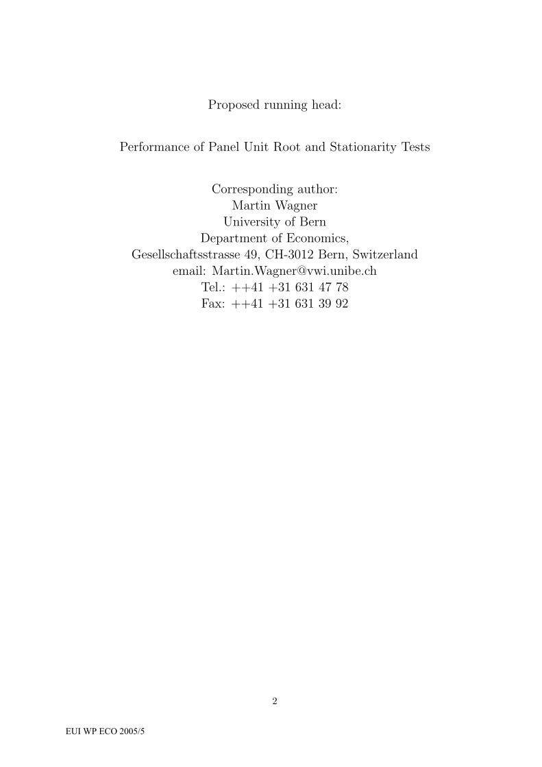
five panel unit root tests designed for serially correlated panels, see Figure 2. In this figure

we display the size performance depending upon the MA parameter c for T = 25.

As a baseline case, and as a follow-up to the previous analysis, we include again the case

c = 0 (the upper left graph of Figure 2). One sees that for short panels (similar results also

hold for T = 10, 15, 20 not shown) in particular the LL932 test and also the MW2 test are

increasingly oversized with increasing N . The two tests of Im, Pesaran and Shin (1997) and

the Breitung (2000) test exhibit satisfactory size behavior. In particular for these three tests

the size is not increasing with N , but stays close to the nominal level of 5%. Note, however,

that for medium length panels with T = 50, 100, both the LL932 test and the MW2 test

exhibit satisfactory size behavior as well (for c = 0). The general summary for the serially

uncorrelated case is that for all T investigated the Im, Pesaran and Shin (1997) tests and the

Breitung (2000) test have comparably acceptable size. The increase is slower for these tests

than for the Levin, Lin and Chu (2002) and the Maddala and Wu (1999) test. Especially

for T small relative to N an application of the Harris and Tzavalis (1999) test offers an

improvement over Levin, Lin and Chu (2002).

For panels with increasingly negative serial correlation, i.e. with c → −0.99, the size

distortions become more prominent for any given T , as is illustrated for T = 25 in Figure 2.

For this value of T , an MA coefficient of c = −0.4 is the ‘boundary’ case (amongst the values of

20


EUI WP ECO 2005/5

c investigated) for which for some tests the size does not rise sharply (i.e. up to 0.2 or higher)

as N is increased to 200. For the more negative values of c, the size diverges for all tests to

1 for N ≥ 100. Somewhat surprising, also for the larger values of T , the ‘boundary’ value

for the MA coefficient is still given by c = −0.4. For T ≥ 50 and for c ∈ {−0.8,−0.9,−.95},‘size divergence’ occurs again for N ≥ 100.20 This divergence can be partly mitigated by

using smaller values for the autoregressive lags than suggested by BIC.21 In light of Table 1,

this divergence might not be too surprising, as most tests’ critical values are derived on

the basis of sequential limit theory. There are, however, exceptions: The Maddala and Wu

test is developed for finite N , and uses an approximation of the p-values for the individual

ADF tests. For serially uncorrelated errors furthermore Im, Pesaran and Shin (1997) provide

critical values for the tests for finite T and only N → ∞. Thus, we a priori expect the MW

test (and the IPS tests for serially uncorrelated errors) to be less prone to the size distortions

observed above. However, this is not observed throughout our simulations. The performance

of the Maddala and Wu test as displayed in Figure 2 is quite representative. For c = 0 it

shows the fastest size divergence for N → 200 and for c �= 0 its size performance is in the ball

park of other tests. What about the two IPS tests? Both tests exhibit rather similar behavior

and their size stays relatively stable close to the nominal value. Of course, for c becoming

too negative some size distortions occur.

The tests that exhibit in most cases the slowest divergence of the size as c is decreased

towards -0.95, are the LL932 and (usually second slowest) the UB2 test. This behavior is

the large T extension of the behavior observed for the Levin, Lin and Chu (2002) test for

small T ∈ {10, 15, 25}. The nominal size of the LL932 test even decreases for fixed small

T ∈ {10, 15, 25} for N tending to 200 for certain values of c (e.g. for T = 25, this holds for

c = −0.2,−0.4). With increasing serial correlation, instead of being undersized this test has

the slowest divergence of the size towards 1 for N → ∞. For the UB2 test the behavior is

different, since it displays relatively fast size divergence for the smaller values of c (see for

an example the center graph in the upper row of Figure 2). Thus, summarizing we find that

for the panels with highly negative MA coefficients, the LL932 test is grosso modo the least20Generally, for very small T = 10, 15 all tests exhibit smaller size distortions as a function of N than for

larger T .21Surprisingly, performing no correction for serial correlation sometimes mitigates the ‘size-divergence’ for

increasing N , in particular for c close to 0. For values of c close to -1, including more lags is in general preferable.The values of c close to -1 also lead, as expected, to larger lag lengths suggested by BIC for T ≥ 100. It is notclear whether these observations have practical implications or generalize beyond the MA(1) error processessimulated in this study. An investigation of this issue is left for future research.

21


EUI WP ECO 2005/5

c=0

0

0.02

0.04

0.06

0.08

0.1

0.12

0.14

0.16

0.18

0.2

10 15 20 25 50 100 200

N

c=-0.2

0

0.02

0.04

0.06

0.08

0.1

0.12

0.14

0.16

0.18

0.2

10 15 20 25 50 100 200

N

c=-0.4

0

0.1

0.2

0.3

0.4

0.5

0.6

10 15 20 25 50 100 200

Nc=-0.8

0

0.1

0.2

0.3

0.4

0.5

0.6

0.7

0.8

0.9

1

10 15 20 25 50 100 200

N

c=-0.9

0

0.1

0.2

0.3

0.4

0.5

0.6

0.7

0.8

0.9

1

10 15 20 25 50 100 200

N

c=-0.95

0

0.1

0.2

0.3

0.4

0.5

0.6

0.7

0.8

0.9

1

10 15 20 25 50 100 200

N

Figure 2: Size of panel unit root tests for case 2 (DGP2(0, 1, c)) with c ∈{0,−0.2,−0.4,−0.8,−0.9,−0.95} for T = 25. The solid lines with bullets correspond toLL932, the solid lines with triangles correspond to UB2, the solid lines correspond to IPSt,2,the dash-dotted lines correspond to IPSLM,2, and the dashed lines correspond to MW2.

distorted test, with in general a slight tendency for being undersized in small T and large N

panels.

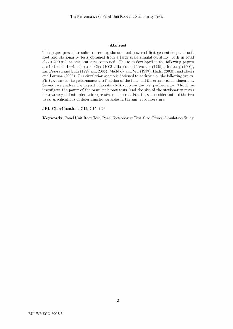
We now turn to case 3 and start again with a comparison of the Levin, Lin and Chu

(2002) and Harris and Tzavalis (1999) tests for c = 0. In Figure 3 we display as above results

for T ∈ {10, 25, 100}. As in the case of random walks without drift, substantially smaller size

distortions are observed for the Harris and Tzavalis (1999) test (in particular again for small

T ). The differences for the larger values of T are slightly less pronounced than in case 2. For

T ≥ 50, the size performance is very satisfactory also for large values of N .

In case of no serial correlation in uit size divergence only occurs for T = 10, 15 for the

LL933 test and at a lesser rate for the MW3 test. For T = 25 all tests except the MW3 test

22


EUI WP ECO 2005/5

T=10

0

0.1

0.2

0.3

0.4

0.5

0.6

0.7

0.8

0.9

1

10 15 20 25 50 100 200

N

T=25

0

0.01

0.02

0.03

0.04

0.05

0.06

0.07

0.08

0.09

10 15 20 25 50 100 200

N

T=100

0

0.01

0.02

0.03

0.04

0.05

0.06

0.07

0.08

0.09

10 15 20 25 50 100 200

N

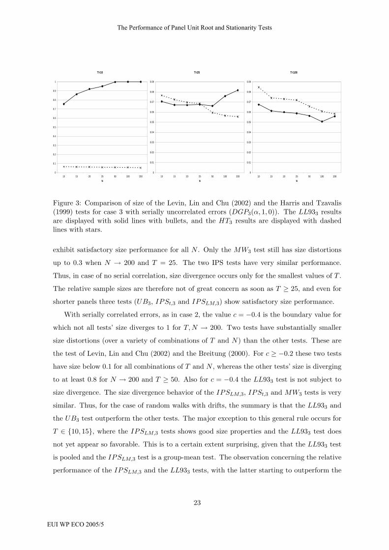
Figure 3: Comparison of size of the Levin, Lin and Chu (2002) and the Harris and Tzavalis(1999) tests for case 3 with serially uncorrelated errors (DGP3(α, 1, 0)). The LL933 resultsare displayed with solid lines with bullets, and the HT3 results are displayed with dashedlines with stars.

exhibit satisfactory size performance for all N . Only the MW3 test still has size distortions

up to 0.3 when N → 200 and T = 25. The two IPS tests have very similar performance.

Thus, in case of no serial correlation, size divergence occurs only for the smallest values of T .

The relative sample sizes are therefore not of great concern as soon as T ≥ 25, and even for

shorter panels three tests (UB3, IPSt,3 and IPSLM,3) show satisfactory size performance.

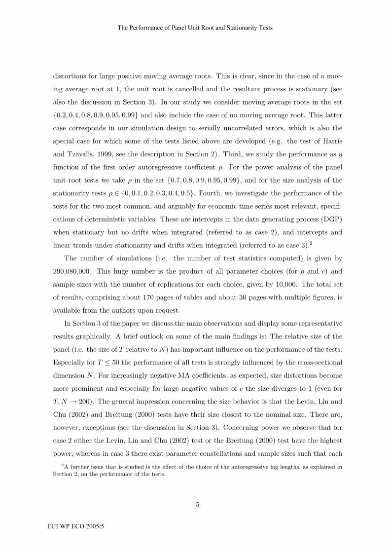
With serially correlated errors, as in case 2, the value c = −0.4 is the boundary value for

which not all tests’ size diverges to 1 for T, N → 200. Two tests have substantially smaller

size distortions (over a variety of combinations of T and N) than the other tests. These are

the test of Levin, Lin and Chu (2002) and the Breitung (2000). For c ≥ −0.2 these two tests

have size below 0.1 for all combinations of T and N , whereas the other tests’ size is diverging

to at least 0.8 for N → 200 and T ≥ 50. Also for c = −0.4 the LL933 test is not subject to

size divergence. The size divergence behavior of the IPSLM,3, IPSt,3 and MW3 tests is very

similar. Thus, for the case of random walks with drifts, the summary is that the LL933 and

the UB3 test outperform the other tests. The major exception to this general rule occurs for

T ∈ {10, 15}, where the IPSLM,3 tests shows good size properties and the LL933 test does

not yet appear so favorable. This is to a certain extent surprising, given that the LL933 test

is pooled and the IPSLM,3 test is a group-mean test. The observation concerning the relative

performance of the IPSLM,3 and the LL933 tests, with the latter starting to outperform the

23


EUI WP ECO 2005/5

c=0

0

0.01

0.02

0.03

0.04

0.05

0.06

0.07

0.08

0.09

10 15 20 25 50 100 200

N

c=-0.2

0

0.01

0.02

0.03

0.04

0.05

0.06

0.07

0.08

0.09

0.1

10 15 20 25 50 100 200

N

c=-0.4

0

0.1

0.2

0.3

0.4

0.5

0.6

0.7

0.8

0.9

1

10 15 20 25 50 100 200

N

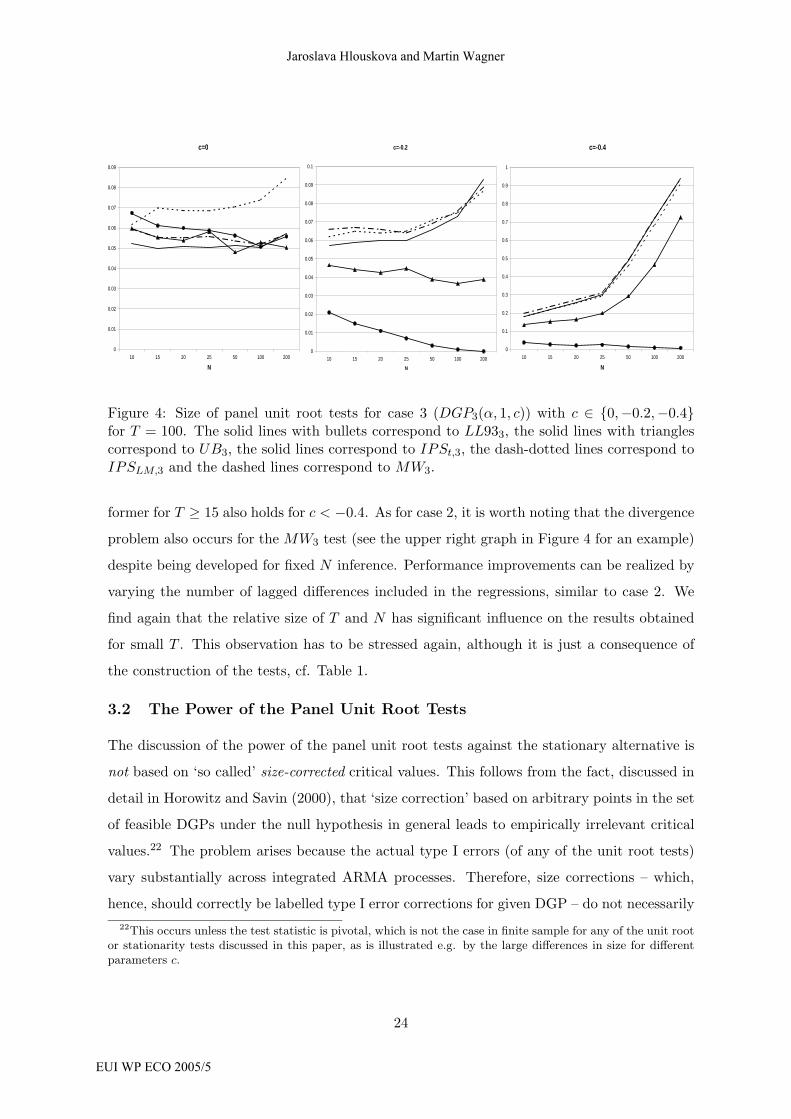
Figure 4: Size of panel unit root tests for case 3 (DGP3(α, 1, c)) with c ∈ {0,−0.2,−0.4}for T = 100. The solid lines with bullets correspond to LL933, the solid lines with trianglescorrespond to UB3, the solid lines correspond to IPSt,3, the dash-dotted lines correspond toIPSLM,3 and the dashed lines correspond to MW3.

former for T ≥ 15 also holds for c < −0.4. As for case 2, it is worth noting that the divergence

problem also occurs for the MW3 test (see the upper right graph in Figure 4 for an example)

despite being developed for fixed N inference. Performance improvements can be realized by

varying the number of lagged differences included in the regressions, similar to case 2. We

find again that the relative size of T and N has significant influence on the results obtained

for small T . This observation has to be stressed again, although it is just a consequence of

the construction of the tests, cf. Table 1.

3.2 The Power of the Panel Unit Root Tests

The discussion of the power of the panel unit root tests against the stationary alternative is

not based on ‘so called’ size-corrected critical values. This follows from the fact, discussed in

detail in Horowitz and Savin (2000), that ‘size correction’ based on arbitrary points in the set

of feasible DGPs under the null hypothesis in general leads to empirically irrelevant critical

values.22 The problem arises because the actual type I errors (of any of the unit root tests)

vary substantially across integrated ARMA processes. Therefore, size corrections – which,

hence, should correctly be labelled type I error corrections for given DGP – do not necessarily22This occurs unless the test statistic is pivotal, which is not the case in finite sample for any of the unit root

or stationarity tests discussed in this paper, as is illustrated e.g. by the large differences in size for differentparameters c.

24


EUI WP ECO 2005/5

lead to insights that can be generalized.

Therefore our power analysis is based on the asymptotic critical values. Horowitz and

Savin (2000) discuss situations when bootstrap based critical values lead to considerable power

gains, this is not discussed here, but the interested reader will find bootstrap applications

of the tests discussed in this paper in Wagner and Hlouskova (2004). The bootstrap based

inference in that paper often leads to different conclusions than inference based on asymptotic

critical values.

Before we discuss the results, let us start by summarizing a few general observations. First,

maybe not surprising, power is monotonically increasing in N for all DGPs simulated under

the stationary alternative for all values of T (see for example Figures 5 and 8). Note, however,

that power does not increase monotonically in T for given N . This occurs for relatively small

values of T and N , when ρ assumes values close to 1. For larger values of T power increases

when T is increased further for any value of N . Most notably the LL93 test is subject to

non-monotonicity of power in T .

We start our discussion again with case 2, see Figure 5. In this figure we display the power

of the panel unit root tests for ρ = 0.8 and T ∈ {10, 25, 100}. The upper row shows the case

with serially uncorrelated errors and the lower row displays the case c = −0.4. The figure

clearly displays one representative result, namely the effect of the value of c on the ordering

of the tests with respect to power. The highest power curve corresponds throughout to either

the UB2 or the LL932 test (also for parameter choices not displayed in figures here). For the

larger values of T it is generally the UB2 test that has highest power, whereas the LL932 test

has highest power in many cases for smaller values of T . Corresponding to the sensitivity

discussed in the previous subsection, altering the lag lengths in the ADF regressions can be

used to improve the power performance of the Levin, Lin and Chu (2002) test. The most

variable power performance is observed for the MW2 test, who is ranked from second to last

place without any detectable dependence upon sample size or parameters (see Figure 5). For

the two group-mean tests of Im, Pesaran and Shin, power is comparatively low for small values

of T (this is most likely a consequence of the group-mean construction of the test statistic),

but is in general quite appealing for larger values of T . However, the UB2 test is for those

large panels the most powerful test. Note also that for T ≥ 100 even for N = 10 all tests have

power equal to 1, for ρ ≤ 0.9. For even larger values of ρ ∈ {0.95, 0.99}, N ≥ 50 is required

to have power tending to 1 for T ≥ 100. The previous observations holds both for c = 0 and

25


EUI WP ECO 2005/5

c �= 0.

c=0, T=10

0

0.1

0.2

0.3

0.4

0.5

0.6

0.7

0.8

0.9

1

10 15 20 25 50 100 200

N

c=0, T=25

0

0.1

0.2

0.3

0.4

0.5

0.6

0.7

0.8

0.9

1

10 15 20 25 50 100 200

N

c=0, T=100

0

0.1

0.2

0.3

0.4

0.5

0.6

0.7

0.8

0.9

1

10 15 20 25 50 100 200

Nc=-0.4, T=10

0

0.1

0.2

0.3

0.4

0.5

0.6

0.7

0.8

0.9

1

10 15 20 25 50 100 200

N

c=-0.4, T=25

0

0.1

0.2

0.3

0.4

0.5

0.6

0.7

0.8

0.9

1

10 15 20 25 50 100 200

N

c=-0.4, T=100

0

0.1

0.2

0.3

0.4

0.5

0.6

0.7

0.8

0.9

1

10 15 20 25 50 100 200

N

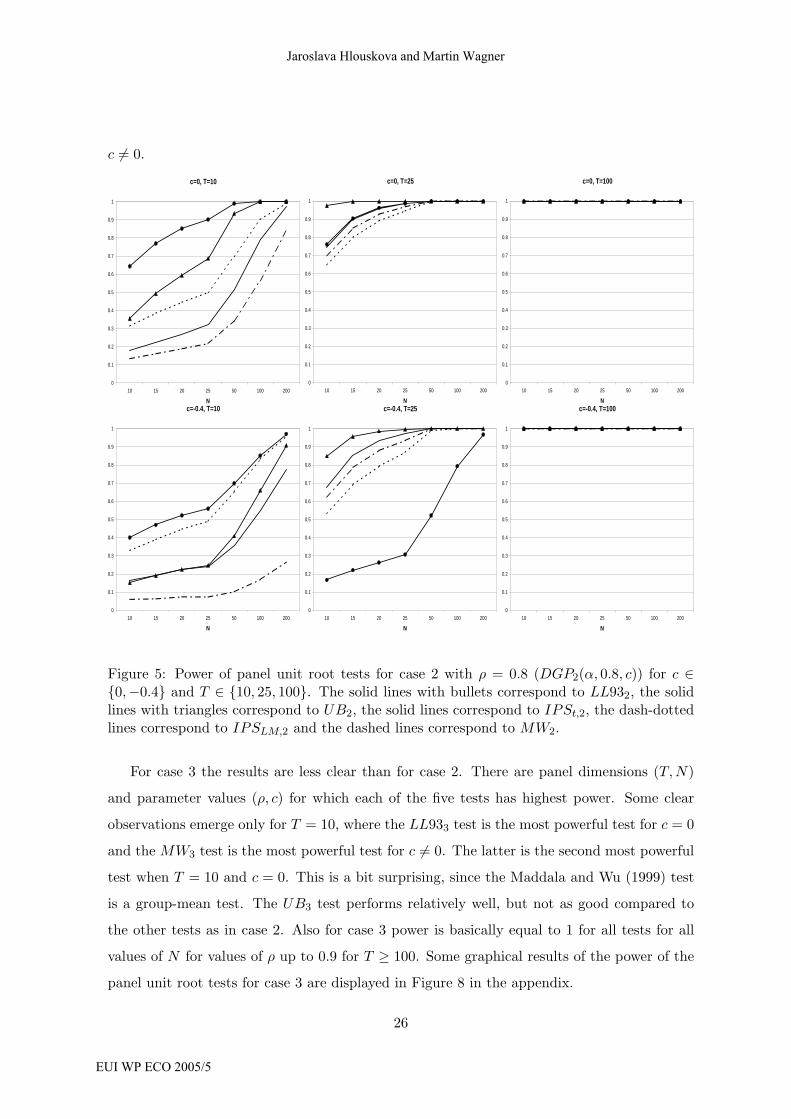
Figure 5: Power of panel unit root tests for case 2 with ρ = 0.8 (DGP2(α, 0.8, c)) for c ∈{0,−0.4} and T ∈ {10, 25, 100}. The solid lines with bullets correspond to LL932, the solidlines with triangles correspond to UB2, the solid lines correspond to IPSt,2, the dash-dottedlines correspond to IPSLM,2 and the dashed lines correspond to MW2.

For case 3 the results are less clear than for case 2. There are panel dimensions (T, N)

and parameter values (ρ, c) for which each of the five tests has highest power. Some clear

observations emerge only for T = 10, where the LL933 test is the most powerful test for c = 0

and the MW3 test is the most powerful test for c �= 0. The latter is the second most powerful

test when T = 10 and c = 0. This is a bit surprising, since the Maddala and Wu (1999) test

is a group-mean test. The UB3 test performs relatively well, but not as good compared to

the other tests as in case 2. Also for case 3 power is basically equal to 1 for all tests for all

values of N for values of ρ up to 0.9 for T ≥ 100. Some graphical results of the power of the

panel unit root tests for case 3 are displayed in Figure 8 in the appendix.

26


EUI WP ECO 2005/5

3.3 The Size of the Panel Stationarity Tests

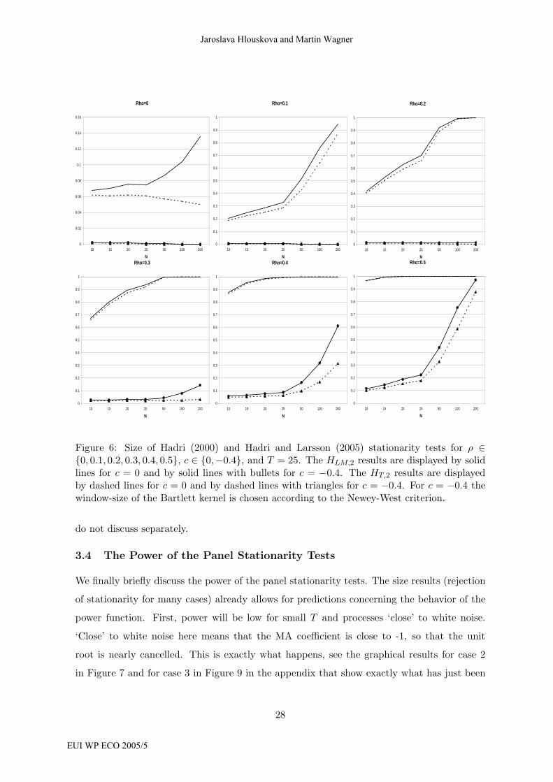
Some representative results for the size behavior of the stationarity tests of Hadri (2000) and

Hadri and Larsson (2005) are displayed in Figure 6 for case 2. The figure displays the size

of both tests as a function of ρ ∈ {0, 0.1, 0.2, 0.3, 0.4, 0.5} and c ∈ {0,−0.4} for T = 25.

Remember from the discussion in Section 2.2 that the HT test of Hadri and Larsson (2005)

is based on finite T inference.

One of the aspects we want to compare is the relative performance of the HT and the HLM

test of Hadri (2000). Focusing on this aspect first, we find that only for the case ρ = 0 and

c = 0 substantial differences between these two tests occur. This holds not only for T = 25

shown, but for all values of T . As expected, for larger values of T , the differences become

smaller. The explanation for this result is that the non-parametric estimation to allow for

serial correlation is too imprecise to result in improved size performance, since advantages

of the HT test only materialize in the single case where no serial correlation corrections are

required.

The second general observation that is exemplified in Figure 6 is that c = 0 leads to larger

size distortions than c < 0, as shown with the example c = −0.4 in the figure. This finding

can be explained by noting that our generated processes are for ρ = 0.4 and c = −0.4 white

noise processes, since the AR and the MA root are cancelled in this case. Thus, it seems

that only for processes ‘close to white noise’ the size of the tests is acceptable.23 This is

bad news since, in case of stationary autoregressive time series with strong serial first order

autocorrelation, the tests have basically size 1. This finding also holds for larger values of T .

Our observation, however, can explain to a certain extent the fact that an application of the

panel stationarity tests a la Hadri (2000), often leads to a rejection of the null hypothesis.

Even for ‘highly stationary panels’ as displayed in the figure, the null is rejected in almost

all replications (unless the AR and the MA root are nearly or exactly cancelled). In other

words, the Hadri (2000) and the Hadri and Larsson (2005) test can be ‘used to find unit roots’

(although, of course, strictly speaking a rejection of the null does not imply acceptance of the

alternative).

Note that qualitatively entirely similar findings are obtained for case 3, which we therefore23The difference to the white noise case displayed in the upper left graph and again in the middle graph in

the lower row (also white noise) is entirely attributable to the non-parametric correction. For c close to -1, asexpected large size distortions occur throughout.

27


EUI WP ECO 2005/5

Rho=0

0

0.02

0.04

0.06

0.08

0.1

0.12

0.14

0.16

10 15 20 25 50 100 200

N

Rho=0.1

0

0.1

0.2

0.3

0.4

0.5

0.6

0.7

0.8

0.9

1

10 15 20 25 50 100 200

N

Rho=0.2

0

0.1

0.2

0.3

0.4

0.5

0.6

0.7

0.8

0.9

1

10 15 20 25 50 100 200

NRho=0.3

0

0.1

0.2

0.3

0.4

0.5

0.6

0.7

0.8

0.9

1

10 15 20 25 50 100 200

N

Rho=0.4

0

0.1

0.2

0.3

0.4

0.5

0.6

0.7

0.8

0.9

1

10 15 20 25 50 100 200

N

Rho=0.5

0

0.1

0.2

0.3

0.4

0.5

0.6

0.7

0.8

0.9

1

10 15 20 25 50 100 200

N

Figure 6: Size of Hadri (2000) and Hadri and Larsson (2005) stationarity tests for ρ ∈{0, 0.1, 0.2, 0.3, 0.4, 0.5}, c ∈ {0,−0.4}, and T = 25. The HLM,2 results are displayed by solidlines for c = 0 and by solid lines with bullets for c = −0.4. The HT,2 results are displayedby dashed lines for c = 0 and by dashed lines with triangles for c = −0.4. For c = −0.4 thewindow-size of the Bartlett kernel is chosen according to the Newey-West criterion.

do not discuss separately.

3.4 The Power of the Panel Stationarity Tests

We finally briefly discuss the power of the panel stationarity tests. The size results (rejection

of stationarity for many cases) already allows for predictions concerning the behavior of the

power function. First, power will be low for small T and processes ‘close’ to white noise.

‘Close’ to white noise here means that the MA coefficient is close to -1, so that the unit

root is nearly cancelled. This is exactly what happens, see the graphical results for case 2

in Figure 7 and for case 3 in Figure 9 in the appendix that show exactly what has just been

28


EUI WP ECO 2005/5

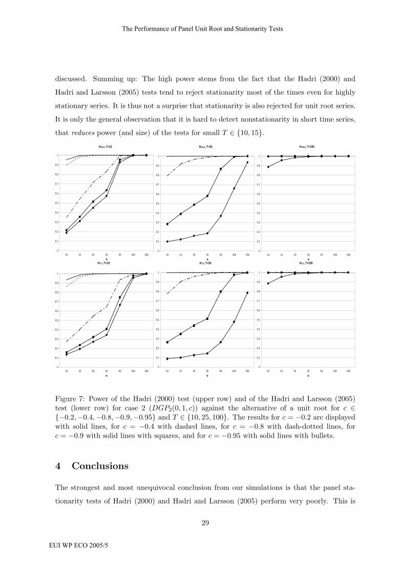
discussed. Summing up: The high power stems from the fact that the Hadri (2000) and

Hadri and Larsson (2005) tests tend to reject stationarity most of the times even for highly

stationary series. It is thus not a surprise that stationarity is also rejected for unit root series.

It is only the general observation that it is hard to detect nonstationarity in short time series,

that reduces power (and size) of the tests for small T ∈ {10, 15}.HLM,2, T=10

0

0.1

0.2

0.3

0.4

0.5

0.6

0.7

0.8

0.9

1

10 15 20 25 50 100 200

N

HLM,2, T=25

0

0.1

0.2

0.3

0.4

0.5

0.6

0.7

0.8

0.9

1

10 15 20 25 50 100 200

N

HLM,2, T=100

0

0.1

0.2

0.3

0.4

0.5

0.6

0.7

0.8

0.9

1

10 15 20 25 50 100 200

NHT,2, T=10

0

0.1

0.2

0.3

0.4

0.5

0.6

0.7

0.8

0.9

1

10 15 20 25 50 100 200

N

HT,2, T=25

0

0.1

0.2

0.3

0.4

0.5

0.6

0.7

0.8

0.9

1

10 15 20 25 50 100 200

N

HT,2, T=100

0

0.1

0.2

0.3

0.4

0.5

0.6

0.7

0.8

0.9

1

10 15 20 25 50 100 200

N

Figure 7: Power of the Hadri (2000) test (upper row) and of the Hadri and Larsson (2005)test (lower row) for case 2 (DGP2(0, 1, c)) against the alternative of a unit root for c ∈{−0.2,−0.4,−0.8,−0.9,−0.95} and T ∈ {10, 25, 100}. The results for c = −0.2 are displayedwith solid lines, for c = −0.4 with dashed lines, for c = −0.8 with dash-dotted lines, forc = −0.9 with solid lines with squares, and for c = −0.95 with solid lines with bullets.

4 Conclusions

The strongest and most unequivocal conclusion from our simulations is that the panel sta-

tionarity tests of Hadri (2000) and Hadri and Larsson (2005) perform very poorly. This is

29


EUI WP ECO 2005/5

to a certain extent similar to the often observed poor performance of the Kwiatkowski et al.

(1992) test, which is the time series building block of these tests. The null of stationarity

is rejected as soon as sizeable serial correlation of either the autoregressive or the moving

average type is present.

The picture that emerges for the panel unit root tests is much more differentiated and only

few clear-cut patterns emerge (which is itself an interesting observation). Some of the main

findings are: First, for case 2 (with intercepts under stationarity) the best power behavior

is displayed by either the Levin, Lin and Chu (2002) test or by the Breitung (2000) test.

Second, for serially uncorrelated panels the Harris and Tzavalis (1999) implementation of

the Levin, Lin and Chu (2002) test offers substantial improvements for short panels. The

third clear message that emerges from the simulations is that for short panels size and power

problems emerge when the cross-sectional dimension is too large, i.e. when T is too small

compared to N . This finding is in line with the fact that most test statistics are based on

sequential limits with first T → ∞ followed by N → ∞. However, the test of Maddala

and Wu (1999), developed for fixed-N inference, does not show superior performance with

respect to variations of N , e.g. concerning size divergence as a function of N . Fourth, as

expected the size distortions become larger when the moving average coefficient c → −1.

Across our simulations the value of c = −0.4 has emerged as a ‘boundary’ case for which

at least some tests exhibit satisfactory behavior (for T ≥ 25 and all values of N). Taking

a rough average over all experiments the Levin, Lin and Chu (2002) and Breitung (2000)

tests have the smallest size distortions. However, there is large variance around this result

and there are constellations where e.g the Levin, Lin and Chu (2002) has very rapid size

divergence. Combined with the good power performance (notably for case 2) those two tests

appear grosso modo quite favorable.

At this point, however, we have to note again that the group-mean tests of Im, Pesaran and

Shin (1997 and 2003) and of Maddala and Wu (1999) are to a certain extent disadvantaged

in our simulation study. This stems from the fact that we simulate (up to the intercepts and

trend slopes) homogenous panels under both the null and the alternative. For such panels

pooling is apparently both advantageous and straightforward. When comparing only the

group-mean tests, we do not find a stable ranking over parameter values and sample sizes,

neither with respect to size nor with respect to power. However, only a detailed analysis

with heterogeneous panels will allow to understand the relative performance of these tests for

30


EUI WP ECO 2005/5

situations where the additional degree of freedom they offer (the heterogeneous alternative)

is utilized

The impact of lag length selection in the ADF type regressions, which has found to be

‘non-monotonous’ in c, is an open issue for future research. By non-monotonicity we mean

the observation that for c close to 0 smaller lag lengths than suggested by BIC lead in many

cases to improved performance, whereas for values of c close to -1 a larger number of lagged

differences than suggested by BIC often leads to improvements. A priori such behavior is

not expected. In this respect also the influence of the time dimension of the panel on this

observation has to be investigated further.

Finally, the variability of the results over the parameters, observed not only for small but

also for large panels, suggests that substantial performance improvements might be realized

by relying upon bootstrap inference.

31


EUI WP ECO 2005/5

Appendix: Additional Figures

Rho=0.7

0

0.1

0.2

0.3

0.4

0.5

0.6

0.7

0.8

0.9

1

10 15 20 25 50 100 200

N

Rho=0.8

0

0.1

0.2

0.3

0.4

0.5

0.6

0.7

0.8

0.9

1

10 15 20 25 50 100 200

N

Rho=0.9

0

0.1

0.2

0.3

0.4

0.5

0.6

0.7

0.8

0.9

1

10 15 20 25 50 100 200

NRho=0.95

0

0.1

0.2

0.3

0.4

0.5

0.6

0.7

0.8

0.9

1

10 15 20 25 50 100 200

N

Rho=0.99

0

0.1

0.2

0.3

0.4

0.5

0.6

0.7

0.8

0.9

1

10 15 20 25 50 100 200

N

Figure 8: Power of panel of unit root tests for case 3 with ρ ∈ {0.7, 0.8, 0.9, 0.95, 0.99} forT = 25 and c = 0 (DGP3(α, ρ, 0)). The solid lines with bullets correspond to LL933, the solidlines with triangles correspond to UB3, the solid lines correspond to IPSt,3, the dash-dottedlines correspond to IPSLM,3 and the dashed lines correspond to MW3.

32


EUI WP ECO 2005/5

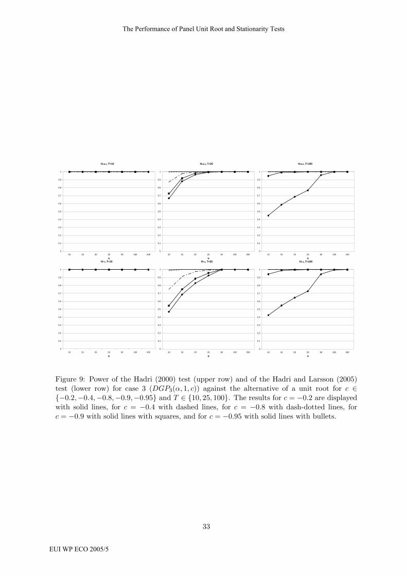
HLM,3, T=10

0

0.1

0.2

0.3

0.4

0.5

0.6

0.7

0.8

0.9

1

10 15 20 25 50 100 200

N

HLM,3, T=25

0

0.1

0.2

0.3

0.4

0.5

0.6

0.7

0.8

0.9

1

10 15 20 25 50 100 200

N

HLM,3, T=100

0

0.1

0.2

0.3

0.4

0.5

0.6

0.7

0.8

0.9

1

10 15 20 25 50 100 200

NHT,3, T=10

0

0.1

0.2

0.3

0.4

0.5

0.6

0.7

0.8

0.9

1

10 15 20 25 50 100 200

N

V

HT,3, T=25

0

0.1

0.2

0.3

0.4

0.5

0.6

0.7

0.8

0.9

1

10 15 20 25 50 100 200

N

HT,3, T=100

0

0.1

0.2

0.3

0.4

0.5

0.6

0.7

0.8

0.9

1

10 15 20 25 50 100 200

N

Figure 9: Power of the Hadri (2000) test (upper row) and of the Hadri and Larsson (2005)test (lower row) for case 3 (DGP3(α, 1, c)) against the alternative of a unit root for c ∈{−0.2,−0.4,−0.8,−0.9,−0.95} and T ∈ {10, 25, 100}. The results for c = −0.2 are displayedwith solid lines, for c = −0.4 with dashed lines, for c = −0.8 with dash-dotted lines, forc = −0.9 with solid lines with squares, and for c = −0.95 with solid lines with bullets.

33


EUI WP ECO 2005/5

References

Agiakloglou, C., Newbold, P. (1996). The balance between size and power in Dickey-Fuller

tests with data-dependent rules for the choice of truncation lag. Economics Letters 56,

229–234.

Andrews, D.W.K. (1991). Heteroskedasticity and autocorrelation consistent covariance matrix

estimation. Econometrica 59, 817–858.

Bai, J., Ng, S. (2004). A PANIC attack on unit roots and cointegration. Econometrica 72,

1127–1178.

Breitung, J. (2000). The local power of some unit root tests for panel data. In: Nonstation-

ary Panels, Panel Cointegration, and Dynamic Panels, Baltagi, B.H. (Ed.), Elsevier,

Amsterdam, pp. 161–177.

Breitung, J., Das, S. (2005). Panel unit root tests under cross sectional dependence. Forth-

coming in Statistica Neerlandica.

Chang, Y. (2002). Nonlinear IV unit root tests in panels with cross-sectional dependency.

Journal of Econometrics 110, 261–292.

Chiang, M-H., Kao, C. (2002). Nonstatonary panel time series using NPT: A user guide.

Center for Policy Research, Syracuse University.

Choi, I. (2001). Unit root tests for panel data. Journal of International Money and Finance

20, 249–272.

Choi, I. (2002). Combination unit root tests for cross-sectionally correlated panels. Forthcom-

ing in: Corbae, D., Durlauf, S., Hansen, B. (Eds.) Econometric Theory and Practice:

Frontiers of Analysis and Applied Research: Essays in Honor of Peter C. B. Phillips,

Cambridge University Press.

Fisher, R.A. (1932). Statistical Methods for Research Workers. Oliver and Boyd, Edinburgh.

Hadri, K. (2000). Testing for stationarity in heterogeneous panel data. Econometrics Journal

3, 148–161.

34


EUI WP ECO 2005/5

Hadri, K., Larsson, R. (2005). Testing for stationarity in heterogeneous panel data where the

time dimension is fixed. Econometrics Journal 8, 55–69.

Harris, R.D.F., Tzavalis, E. (1999). Inference for unit roots in dynamic panels where the time

dimension is fixed. Journal of Econometrics 90, 1–44.

Horowitz, J.L., Savin, E.N. (2000). Empirically relevant critical values for hypothesis tests:

A bootstrap approach. Journal of Econometrics 95, 375–389.

Im, K.S., Pesaran, M.H., Shin, Y. (1997). Testing for unit roots in heterogeneous panels.

Mimeo.

Im, K.S., Pesaran, M.H., Shin, Y. (2003). Testing for unit roots in heterogeneous panels.

Journal of Econometrics 115, 53–74.

Karlsson, S., Lothgren, M. (2000). On the power and interpretation of panel unit root tests.

Economics Letters 66, 249–255.

Kwiatkowski, D., Phillips, P.C.B., Schmidt, P., Shin, Y. (1992). Testing the null hypothesis of

stationarity against the alternative of a unit root. Journal of Econometrics 54, 91–115.

Levin, A., Lin, C.F. (1992). Unit root tests in panel data: Asymptotic and finite sample

properties. UC San Diego Working Paper 92-23.

Levin, A., Lin, C.F. (1993). Unit root tests in panel data: New results. UC San Diego Working

Paper 93-56.

Levin, A., Lin, C.F., Chu, C-S.J. (2002). Unit root tests in panel data: Asymptotic and finite

sample properties. Journal of Econometrics 108, 1–22.

MacKinnon, J.G. (1994). Approximate asymptotic distribution functions for unit root and

cointegration tests. Journal of Applied Econometrics 11, 601–618.

Maddala, G.S., Wu, S. (1999). A comparative study of unit root rests with panel data and a

simple new test. Oxford Bulletin of Economics and Statistics 61, 631–652.

Moon, H.R., Perron, B. (2004). Testing for a unit root in panels with dynamic factors. Journal

of Econometrics 122, 81–126.

35


EUI WP ECO 2005/5

Newey, W., West, K.D. (1994). Automatic lag selection for covariance matrix estimation.

Review of Economic Studies 61, 631 – 653.

Pesaran, M.H. (2003). A simple panel unit root test in the presence of cross section depen-

dence. Mimeo, University of Cambridge.

Phillips, P.C.B. (1987). Time series regression with a unit root. Econometrica 55, 277-301.

Phillips, P.C.B., Moon, H.R. (1999). Linear regression limit theory for nonstationary panel

data. Econometrica 67, 1057–1111.

Wagner, M., Hlouskova, J. (2004). What’s really the story with this Balassa-Samuelson effect

in the CEECs? University of Bern, Department of Economics, Discussion Paper 04/16.

36


EUI WP ECO 2005/5

EUROPEAN UNIVERSITY INSTITUTE DEPARTMENT OF ECONOMICS · EUROPEAN UNIVERSITY INSTITUTE DEPARTMENT...

Documents

Transcript of EUROPEAN UNIVERSITY INSTITUTE DEPARTMENT OF ECONOMICS · EUROPEAN UNIVERSITY INSTITUTE DEPARTMENT...