European Patent Office - Orig.: en Munich, …CA/46/19 e 2019-6392 CA/46/19 Orig.: en Munich,...

CA/46/19 e 2019-6392

CA/46/19

Orig.: en

Munich, 10.05.2019

SUBJECT: Financial Study

SUBMITTED BY: President of the European Patent Office

ADDRESSEES: 1. Budget and Finance Committee (for information) 2. Administrative Council (for information)

SUMMARY

Previous financial studies dating back to 2011 and 2016, the Office decided to commission an external independent consultant to perform a new Financial Study assessing the situation of the EPO and its long term sustainability. It is a good management practice to regularly monitor the progress of its financial situation, particularly in a fast evolving environment. The consultant Oliver Wyman ‒ Mercer, selected to perform the study, developed four long-term scenarios and simulated their financial impact, taking due consideration of the developments in the patent and financial landscape since the last financial study (2016). All stakeholders will be given the opportunity to get acquainted with the methodology and outcome of the study. In a second phase starting in Q3 2019, the discussions will focus on the possible ways forward. The Financial Study will be distributed in English language only. Recommendation for publication: Yes.

This document has been issued in electronic form only.

EUROPEAN PATENT OFFICE

FINANCIAL STUDY 2019 – FINAL REPORT

MAY 10, 2019

© Oliver Wyman

CONFIDENTIALITY

Our clients’ industries are extremely competitive, and the maintenance of confidentiality with respect to our clients’ plans and data is critical. Oliver Wyman rigorously applies internal confidentiality practices to protect the confidentiality of all client information.

Similarly, our industry is very competitive. We view our approaches and insights as proprietary and therefore look to our clients to protect our interests in our proposals, presentations, methodologies and analytical techniques. Under no circumstances should this material be shared with any third party without the prior written consent of Oliver Wyman.

© Oliver Wyman

© Oliver Wyman 3

Contents

CONFIDENTIALITY ................................................................................................... 2

Executive Summary ............................................................................................... 10

1. Purpose and context of this document .................................................. 23

1.1. Mandate and purpose of this document ............................................................... 23

1.2. Previous Financial Studies and differences to the 2019 Financial Study .............. 24

1.3. Approach ............................................................................................................. 25

2. Financial and operational status quo ..................................................... 27

2.1. Revenue .............................................................................................................. 27

2.2. Total expenses..................................................................................................... 28

2.3. Total Equity .......................................................................................................... 31

2.4. Cash flow ............................................................................................................. 32

2.5. Productivity, SEO Production and stock ............................................................... 33

3. Approach and scenario assumptions .................................................... 35

3.1. Methodological approach ..................................................................................... 35

3.2. Introduction of four scenarios ............................................................................... 35

3.3. Identification of external parameters defining the four scenarios .......................... 37

3.4. External parameter values ................................................................................... 37

3.4.1. Deep-Dive: Risk-free interest rate ........................................................................ 43

3.4.2. Deep-Dive: Discount rate ..................................................................................... 44

3.4.3. Deep-Dive: Inflation ............................................................................................. 45

3.4.4. Deep-Dive: Equity Market index ........................................................................... 46

3.4.5. Deep Dive: Credit Spread .................................................................................... 47

3.4.6. Deep Dive: Mortality ............................................................................................. 47

3.5. Incoming Demand ................................................................................................ 48

3.5.1. Demand forecasting model .................................................................................. 48

3.5.2. Model inputs and results – Base 1: Economic Recovery scenario ........................ 48

3.5.3. Model inputs and results – Optimistic scenario..................................................... 50

3.5.4. Model inputs and results – Base 2: Economic Cycle scenario .............................. 51

3.5.5. Model inputs and results – Stress scenario .......................................................... 52

3.5.6. Summary of incoming demand forecast ............................................................... 53

3.6. Internal parameters of the Patent Grant Process ................................................. 54

3.6.1. Target Stock and timeliness ................................................................................. 54

3.6.2. Productivity .......................................................................................................... 56

3.6.3. Workforce ............................................................................................................ 58

3.6.4. Production ............................................................................................................ 59

3.7. Internal financial parameters ................................................................................ 59

3.7.1. Statement of Comprehensive Income .................................................................. 59

3.7.2. Statement of Financial Position ............................................................................ 61

© Oliver Wyman 4

3.7.3. Statement of Cash Flows ..................................................................................... 62

3.7.4. Pension modelling approach and assumptions .................................................... 62

3.7.5. Modelling of RFPSS and EPOTIF ........................................................................ 67

4. Scenario results ....................................................................................... 70

4.1. Key operational forecasts ..................................................................................... 70

4.1.1. Production and published patents ........................................................................ 70

4.1.2. Workforce ............................................................................................................ 71

4.1.3. Stock .................................................................................................................... 72

4.2. Pension results .................................................................................................... 73

4.3. Key financial forecasts ......................................................................................... 74

4.3.1. Statement of Financial Position ............................................................................ 74

4.3.2. Statement of Comprehensive Income .................................................................. 76

4.3.3. Development of revenue from procedural and renewal fees................................. 77

4.3.4. Statement of Cash Flows ..................................................................................... 79

4.4. Coverage gap ...................................................................................................... 81

4.5. Sensitivity analysis to discount rate ...................................................................... 83

4.6. Summary of scenario results ................................................................................ 85

5. Considerations and outlook on managerial actions ............................. 86

Appendix A. IFRS financial statements 2016-2038 ......................................... 87

Appendix B. Assumptions in the financial model ........................................ 111

Appendix C. PESTEL analysis of exogeneous drivers of the EPO’s financial situation ..................................................................................... 124

Appendix D. Demand forecast plausibility check of the EPO Forecast ..... 130

© Oliver Wyman 5

List of Tables

Table 1: Scenarios used in the Financial Study .................................................................................... 36

Table 2: Overview of scenario parameter values ................................................................................. 38

Table 3: Applications forecast: Base 1 scenario ................................................................................... 50

Table 4: Applications forecast: Optimistic scenario .............................................................................. 51

Table 5: Applications forecast: Base 2 scenario ................................................................................... 52

Table 6 Applications forecast: Stress scenario ..................................................................................... 53

Table 7: EPO employee-benefit schemes description .......................................................................... 63

Table 8: Assumption for new entrants .................................................................................................. 66

Table 9: Benefit funding gap, cash surplus & coverage gap in Base 2 scenario .................................. 82

Table 10: Statement of Comprehensive Income: Base 1 scenario ...................................................... 87

Table 11: Statement of Financial Position: Base 1 scenario ................................................................ 89

Table 12: Statement of Cash Flows (Direct approach – Office view): Base 1 scenario ....................... 91

Table 13: Statement of Comprehensive Income: Optimistic scenario .................................................. 93

Table 14: Statement of Financial Position: Optimistic scenario ............................................................ 95

Table 15: Statement of Cash Flows (Direct approach – Office view): Optimistic scenario .................. 97

Table 16: Statement of Comprehensive Income: Base 2 scenario ...................................................... 99

Table 17: Statement of Financial Position: Base 2 scenario .............................................................. 101

Table 18: Statement of Cash Flows (Direct approach – Office view): Base 2 scenario ..................... 103

Table 19: Statement of Comprehensive Income: Stress scenario...................................................... 105

Table 20: Statement of Financial Position: Stress scenario ............................................................... 107

Table 21: Statement of Cash Flows (Direct approach – Office view): Stress scenario ...................... 109

Table 22: Assumptions in the financial model..................................................................................... 111

Table 23: EPO applications actual vs. forecast 2007-2017 (average annual growth rates) ............... 130

© Oliver Wyman 6

List of Figures

Figure 1: Total applications and Products per Head 2016-2018 .......................................................... 11

Figure 2: Development of financial and macroeconomic drivers 2016-2018 ........................................ 12

Figure 3: Economic and financial developments over the 20-year horizon under consideration ......................................................................................................................................... 13

Figure 4: Key operational parameters: timeliness criteria, productivity, workforce............................... 14

Figure 5: Cumulative probability distribution of real returns of the RFPSS 2018-2038 ........................ 15

Figure 6: Annual benefit payments ....................................................................................................... 16

Figure 7: Required assets in 2038 for benefit payments after 2038 ..................................................... 16

Figure 8: Benefit funding gap in 2038 ................................................................................................... 17

Figure 9: Operating cash flow (Direct approach – Office view) – All scenarios forecast [IFRS] .................................................................................................................................................... 18

Figure 10: Coverage gap/ surplus: Benefit funding gap and available cash surplus (cumulative) in 2038 .............................................................................................................................. 19

Figure 11: Revenue and operating cost base 2016 vs. 2018 ............................................................... 20

Figure 12: Possibilities to reduce the coverage gap ............................................................................. 21

Figure 13: Total revenues 2008-2018; By revenue type ....................................................................... 28

Figure 14: Revenue from procedural fees 2008-2018 .......................................................................... 28

Figure 15: Total operating expenses 2008-2018 .................................................................................. 29

Figure 16: Employee benefit expenses and total headcount 2008-2018 ............................................. 30

Figure 17: Current IFRS Pension Service Cost 2008-2018 .................................................................. 30

Figure 18: Total Equity 2008-2018 ........................................................................................................ 31

Figure 19: Cash flow 2008-2018 ........................................................................................................... 32

Figure 20: PpH development 2008-2018 .............................................................................................. 33

Figure 21: SEO production 2008-2018 ................................................................................................. 34

Figure 22: SEO stock 2008-2018 .......................................................................................................... 34

Figure 23: Risk-free rate, 10 years ....................................................................................................... 44

Figure 24: AA discount rate, 26 years ................................................................................................... 44

Figure 25: Price index (inflation) ........................................................................................................... 45

Figure 26: European equity market index ............................................................................................. 47

Figure 27: R&D-to-GDP ratios .............................................................................................................. 49

Figure 28: Applications forecast across all scenarios ........................................................................... 53

Figure 29: Search forecast across all scenarios ................................................................................... 54

Figure 30: Overview over the milestone concept at the EPO ............................................................... 55

Figure 31: Target stock search and examination development ............................................................ 56

Figure 32: Examiner time required per product, 2018–2038 ................................................................ 57

Figure 33: Products per Head, 2018-2038............................................................................................ 58

Figure 34: Real annual payments for closed group .............................................................................. 65

Figure 35: Annual benefit payments ..................................................................................................... 67

Figure 36: Search production by scenario ............................................................................................ 70

Figure 37: Examination and opposition production by scenario ........................................................... 70

Figure 38: Published patents by scenario ............................................................................................. 71

Figure 39: Examiner Workforce development ....................................................................................... 72

Figure 40: Examiner replacement ratio by scenario ............................................................................. 72

Figure 41: Cumulated search and examination stock (cases) .............................................................. 73

Figure 42: Projected IFRS DBO in Base 2 scenario over 20 years ...................................................... 73

© Oliver Wyman 7

Figure 43: Equity – All scenarios forecast [IFRS] ................................................................................. 74

Figure 44: Key components of the Statement of Financial Position – Base 2 scenario ....................... 75

Figure 45: Cash and cash equivalents and other financial assets, All scenarios forecast ................... 75

Figure 46: Operating result – All scenarios forecast ............................................................................ 76

Figure 47: Operating result – Base 2 scenario ..................................................................................... 76

Figure 48: Revenue from Procedural Fees - All scenarios forecast ..................................................... 77

Figure 49: Revenue from Internal Renewal Fees - All scenarios forecast ........................................... 78

Figure 50: Revenue from National Renewal Fees - All scenarios forecast .......................................... 79

Figure 51: Operating cash flow (Direct approach – Office view) – All scenarios forecast ................... 80

Figure 52: Fee cash proceeds and salaries per examiner in K€, Base 2 scenario .............................. 80

Figure 53: Net Operating cash flow per examiner in K€, Base 2 scenario, IFRS view ........................ 81

Figure 54: Coverage gap/ surplus: Benefit funding gap and available cash surplus (cumulative) in 2038 .............................................................................................................................. 81

Figure 55: Equity – All scenarios forecast, AAA Government Bond discount rate ............................... 83

Figure 56: Operating result – All scenarios forecast, AAA Government Bond discount rate ............... 84

Figure 57: Operating cash flow (Direct approach – Office view) – All scenarios forecast, AAA Government Bond discount rate ................................................................................................... 84

Figure 58: Options to reduce the coverage gap ................................................................................... 86

Figure 59: Growth in EPO Applications 1990-2017 ............................................................................ 124

Figure 60: International patent filings by applicant’s country of residence ......................................... 126

© Oliver Wyman 8

List of abbreviations

A Actual

AAG Actuarial Advisory Group

ALM Asset Liability Management

B/S Balance Sheet

BN Billion

bps Basis Point

CAGR Compound Annual Growth Rate

CPI Consumer Price Index

DB Defined Benefit

DBO Defined Benefit Obligation

DC Defined Contribution

DFC Deloitte Forecast

DG Directorate General

DR Discount Rate

ECB European Central Bank

EP European Patent

EPC European Patent Convention

EPO European Patent Office

EPOTIF European Patent Office Treasury Investment Fund

EU European Union

FC Forecast

FTE Full Time Equivalent

GDP Gross Domestic Product

HBC Healthcare, Biotechnology and Chemistry

HC Headcount

HICP Harmonized Index of Consumer Prices (excluding tobacco)

HR Human Resources

IAS International Accounting Standards

ICSLT International Civil Servants Life Table

ICT Information and Communications Technology

IFRS International Financial Reporting Standards

IMF International Monetary Fund

IP5 Denomination of five large intellectual property offices (US Patent and Trademark Office, European Patent Office, Japan Patent Office, Korean Intellectual Property Office, National Intellectual Property Administration in China)

IRF Internal Renewal Fee

ISA International Search Authority

ISRP International Service for Remunerations and Pensions

K Thousand

© Oliver Wyman 9

LTC Long-Term Care

KPI Key Performance Indicator

MAC Management Advisory Committee

MM Mobility and Mechatronics

MMC Marsh & McLennan Companies

MN Million

MTBP Medium Term Business Plan

N/A Not applicable

NPO National Patent Office

NPS New Pension Scheme

NRF National Renewal Fee

OECD Organization for Economic Co-operation and Development

OpEx Operational Expenditure

OPS Old Pension Scheme

OY Ordinal Year

P&L Profit and Loss Statement

p.a. Per annum

P/E Price-earnings ratio

PCT Patent Cooperation Treaty

PGP Patent Grant Process

PO Patent Office

PPE Property, Plant and Equipment

PpH Products per Head

R&D Research and Development

RFPSS Reserve Fund for Pensions and Social Security

S/E Searches per Examinations ratio

SAA Strategic Asset Allocation

SEO Search, Examination, Opposition

SME Small and Medium-sized Enterprise

SSP Salary Savings Plan

TOM Target Operating Model

UP Unitary Patent

YoY Year-on-Year

© Oliver Wyman 10

Executive Summary

Long-term financial sustainability is a prerequisite for the existence of a self-funded organization, such as the European Patent Office (EPO). It is the joint responsibility of the Office towards all staff and all stakeholders to ensure financial sustainability and independence at all times. Thus, since 2011 there is a regular assessment of the Office’s current financial situation and its evolution in the future. To address new business challenges that evolved since the last studies 2010/-11 and in 2016, a 3rd Financial Study was initiated, and Mercer/ Oliver Wyman were mandated to prepare this study.

This summary provides an overview of the context and objectives for the Financial Study, key developments since 2016 that make a new study necessary, key assumptions, and the findings of the analyses conducted between December 2018 and April 2019:

1. Context and objectives of the 2019 Financial Study

A first external Financial Study was published in 2011 with the conclusion that the Office would face financial challenges in the future such as increasing total salary costs comprising basic salaries and social security costs, declining equity and liquidity and the potential need for additional funding. This was reconfirmed by a second external Financial Study in 2016 which assessed the Office’s progress, confirmed that the Office had managed to deliver financial results ahead of those anticipated in the 2011 study, but highlighted that the EPO would still face financial challenges in the future without further action.

Over this period, the Office has succeeded in implementing a comprehensive set of initiatives which have started to address structural financial deficiencies. These initiatives include the introduction of EPOTIF as a long-term liquidity reserve, increased productivity and the introduction of the new employment framework.

However, some events could not fully be anticipated in 2016: a low interest rate environment persists, and the production and productivity of the Patent Granting Process have evolved faster than anticipated. Additionally, annual benefit payments will be higher than contributions to RFPSS sooner than expected.

All these changes reinforce the need for a new Financial Study.

The 2019 Financial Study therefore provides a view on a range of financial scenarios over a 20-year time horizon and an estimate as to whether the EPO can meet all its financial obligations within each scenario. It analyzes the developments since the last study and uses forward looking financial scenarios to forecast a set of financial statements on a 20-year horizon.

This new Financial Study has three differentiating characteristics:

• Firstly, a proprietary financial model was built to forecast the financial statements over a 20-year horizon. As part of the scenario analysis, the results were reconciled with EPO internal bottom-up modelling whenever relevant. Explanations for remaining deviations were investigated if necessary.

• Secondly, the 2019 Financial Study includes an in-depth and comprehensive employee benefit modelling with the objective to ensure that future benefits can be paid out of available cash with an acceptable probability.

• Thirdly, the 2019 Financial Study allows for simulating different performances of the EPOTIF based on capital market scenarios and strategic asset allocation. Similar

© Oliver Wyman 11

performance modelling is also undertaken for the RFPSS, the Reserve Fund for Pensions and Social Security.

2. Financial developments since the previous study

The scenarios in 2016 modelled a range of possible outcomes based on a number of assumptions. The reconciliation of the outputs of these previous scenarios with actual developments ever since reinforces the need to:

• monitor actual development over time and update the Office’s view on key indicators

• develop and refine the top-down model

• be prepared for a wider range of outcomes

Key indicators such as total applications and Products per Head (PpH) have grown significantly over recent years.

Figure 1: Total applications and Products per Head 2016-2018, in K#/ in #, forecast vs. actuals

Source: EPO Financial Statements 2016–2018; Financial Study 2016 Forecast (Base Case 100); Mercer and Oliver Wyman analysis

In contrast to these positive developments, capital markets continue to experience a persistently low interest rate environment. This drives low discount rates which have a negative impact on defined benefit obligations and subsequently equity. Furthermore, due to the low interest rate environment, annual employee benefit expenses such as the pension rights acquired have also grown more strongly than originally anticipated.

© Oliver Wyman 12

Figure 2: Development of financial and macroeconomic drivers 2016-2018, forecast vs. actuals, in %/ in BN€

1. Including family allowance and tax compensation Source: EPO Financial Statements 2016–2018; Financial Study 2016 Forecast (Base Case 100); Mercer and Oliver Wyman analysis

3. Assumptions for the 2019 Financial Study

The 2019 Financial Study takes into consideration explicit assumptions regarding the future development of a) macroeconomic factors, b) operational parameters, and c) employee benefits. These assumptions are summarized below:

a) Macroeconomic scenarios:

Forecasting a 20-year development of the EPO’s financial position is inevitably a very uncertain exercise, as these positions will be impacted by factors which cannot be predicted with certainty. Therefore, four scenarios were developed, defined by a set of external factors (which cannot be influenced by the EPO), that determine the economic environment in which the organization operates:

• Optimistic scenario: Reflecting very favourable economic developments such as high applications growth, high risk assets generating higher than expected returns, equities experience strong earnings

• Base 1 scenario – Economic Recovery: Economic growth development in line with the average of forecasts by international institutions (OECD/ World Bank/ IMF) with interest rates gradually increasing due to an improving economic environment

© Oliver Wyman 13

• Base 2 scenario – Economic Cycle: A global economic recession occurs in 2020 of the magnitude typically assumed by regulatory oversight bodies, followed by a normalization from 2025 onwards

• Stress scenario: Assumptions of the Base 2 scenario, supplemented by Chinese economic growth leading to a relocation of industry and reduction in demand for the EPO

All scenarios represent possible evolutions of the future and illustrate how the Office’s financial situation may differ in more and less favorable economic circumstances. They are not associated with a probability for the future situation nor do they attempt to accurately forecast the future. They show a range of outcomes and the sensitivities of the evolution of the Office in these situations and should not be understood as the only ways in which the Office’s future situation may evolve.

Figure 3: Economic and financial developments over the 20-year horizon under consideration, CAGR 2018-2038/ in%, by scenario

1. CAGR between 2018 and 2038 Source: EPO Financial Statements 2016–2018; Financial Study 2016 Forecast (Base Case 100); Mercer and Oliver Wyman analysis

However, all four scenarios are possible and could materialize over time. The Study purposefully does not model a worst-case crash or a low interest rate environment that persists for the 20-year horizon, but rather focusses on scenarios that the EPO should be prepared for if exercising prudent financial management.

© Oliver Wyman 14

b) Operational parameters (EPO-specific):

In terms of operational parameters, the Financial Study makes the following three key assumptions for timeliness, productivity and workforce underlying each scenario:

• Timeliness: 5 months for search as of 2019 and 25 months for examination in line with Early Certainty criteria (“case view”)

• Productivity: 3% productivity increase over the coming years until 2022. This is reflected in reduced time per product and takes into account the already high starting base to which time per product has evolved over the last years

• Workforce: The replacement ratio for retiring examiners ranges between 0.9 and 2.2 depending on the scenario. A ratio above 1 means that there will be more recruitment than retirement over the 20-years period. This is a result of the increase in productivity and the timeliness criteria which determine the required head count to address demand.

All other operational parameters are assumed to remain constant over time.

Figure 4: Key operational parameters: timeliness criteria, productivity, workforce

1. EPO Case View Source: EPO Financial Statements 2016–2018; Mercer and Oliver Wyman analysis

c) Employee benefits:

In terms of employee benefits valuation, one of the most impactful assumptions is the discount rate used. While IFRS prescribes the use of the yield on high quality corporate bonds, the actuarial valuation carried out every two years by the Actuarial Advisory Group (AAG) uses the expected real return of the RFPSS. The real return is defined as the return on the assets that is achievable in addition to inflation. This return is influenced by capital markets as well as the amount of investment risk taken by the RFPSS.

© Oliver Wyman 15

Given the low interest rate environment and the multitude of risks the global economy faces in the upcoming years, a wide range of potential returns are possible. Based on long-term capital market assumptions, the study forecasts that the RFPSS will only meet the return target of the actuarial valuation conducted in 2017, that is a real return of 3.5%, with a probability of 40%. Therefore, there is a 60% probability that the returns generated by the RFPSS are not as high as assumed necessary to fully cover future benefit payments. In these cases, there would be the need for extraordinary contributions by the Office. Furthermore, a 3.5% real return is higher than usual targets for pensions and other benefits of other institutional investment entities. For prudent management of the EPO, the Financial Study 2019 uses a real return of 2.1% as the target which can be achieved with a significantly higher probability of 66%.

Figure 5: Cumulative probability distribution of real returns of the RFPSS 2018-2038, in %

1. Updated based on revision versus September 2018 RFPSS MICADO publication Source: Mercer and Oliver Wyman analysis

4. Findings and results

The findings of the study can be condensed into six key messages:

a) Pension payments will triple by 2038 and benefit liabilities will not be completely covered by cash reserves in 2038

For the assessment of long-term sustainability, the Financial Study covers funded benefits (pension payments of the OPS and NPS employees will receive after retirement as well as health and long-term care payments – contributions paid to the RFPSS each year) as well as

© Oliver Wyman 16

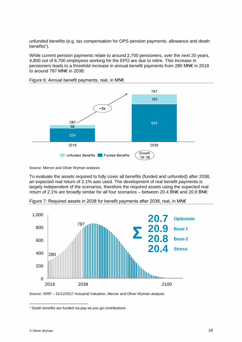
unfunded benefits (e.g. tax compensation for OPS pension payments, allowance and death benefits1).

While current pension payments relate to around 2,700 pensioners, over the next 20 years, 4,800 out of 6,700 employees working for the EPO are due to retire. This increase in pensioners leads to a threefold increase in annual benefit payments from 280 MN€ in 2018 to around 787 MN€ in 2038:

Figure 6: Annual benefit payments, real, in MN€

Source: Mercer and Oliver Wyman analysis

To evaluate the assets required to fully cover all benefits (funded and unfunded) after 2038, an expected real return of 2.1% was used. The development of real benefit payments is largely independent of the scenarios, therefore the required assets using the expected real return of 2.1% are broadly similar for all four scenarios – between 20.4 BN€ and 20.9 BN€:

Figure 7: Required assets in 2038 for benefit payments after 2038, real, in MN€

Source: ISRP – 31/12/2017 Actuarial Valuation, Mercer and Oliver Wyman analysis

1 Death benefits are funded via pay-as-you go contributions

800

0

600

200

1,000

400 280

787

2018 2038 2100

20.720.920.820.4

Optimistic

Base 1

Base 2

Stress

Σ

© Oliver Wyman 17

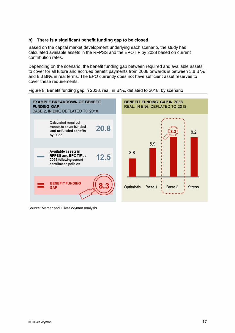
b) There is a significant benefit funding gap to be closed

Based on the capital market development underlying each scenario, the study has calculated available assets in the RFPSS and the EPOTIF by 2038 based on current contribution rates.

Depending on the scenario, the benefit funding gap between required and available assets to cover for all future and accrued benefit payments from 2038 onwards is between 3.8 BN€ and 8.3 BN€ in real terms. The EPO currently does not have sufficient asset reserves to cover these requirements.

Figure 8: Benefit funding gap in 2038, real, in BN€, deflated to 2018, by scenario


© Oliver Wyman 18

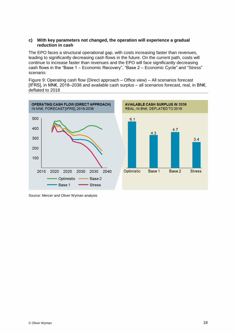
c) With key parameters not changed, the operation will experience a gradual reduction in cash

The EPO faces a structural operational gap, with costs increasing faster than revenues, leading to significantly decreasing cash flows in the future. On the current path, costs will continue to increase faster than revenues and the EPO will face significantly decreasing cash flows in the “Base 1 – Economic Recovery”, “Base 2 – Economic Cycle” and “Stress” scenario:

Figure 9: Operating cash flow (Direct approach – Office view) – All scenarios forecast [IFRS], in MN€, 2018–2038 and available cash surplus – all scenarios forecast, real, in BN€, deflated to 2018


© Oliver Wyman 19

Figure 10 compares the benefit funding gap to the available cash surplus. In all but the optimistic scenario there is still a gap called the coverage gap which is used in the Financial Study to compare the scenarios:

Figure 10: Coverage gap/ surplus: Benefit funding gap and available cash surplus (cumulative) in 2038, real, in MN€, deflated to 2018


The gap is heavily influenced by the conditions assumed in each scenario with a negative coverage gap (ranging from -1.6 BN€ to -4.8 BN€) in all but the optimistic scenario. The Study therefore demonstrates that, unless very optimistic macroeconomic assumptions materialize, a prudent assessment indicates that the Office is likely to experience a structural coverage gap in 2038.

Please note that the calculation of the coverage gap/ surplus is a purely cash-based view and as such not driven by considerations of the applied accounting standards.

d) A time-limited window of opportunity to act is open now

The window of opportunity to build up necessary reserves and financial buffer is open now whilst the EPO’s cash flow is still sufficiently high. The EPO can use this to build up asset reserves to increase the probability that asset returns can fully cover future and accrued benefits payments from the current probability of ~40% to ~66%. Each year during which these actions are deferred will negatively impact the probability that benefit payments will be fully funded in the long-term.

© Oliver Wyman 20

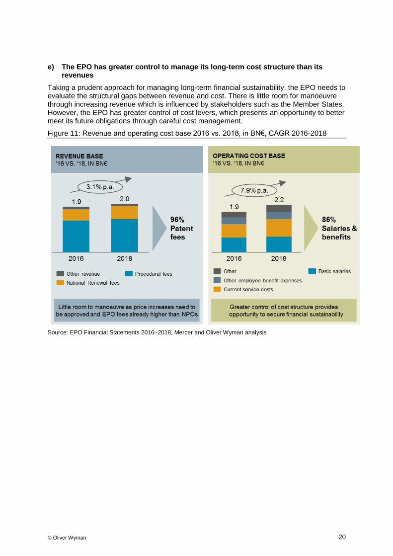
e) The EPO has greater control to manage its long-term cost structure than its revenues

Taking a prudent approach for managing long-term financial sustainability, the EPO needs to evaluate the structural gaps between revenue and cost. There is little room for manoeuvre through increasing revenue which is influenced by stakeholders such as the Member States. However, the EPO has greater control of cost levers, which presents an opportunity to better meet its future obligations through careful cost management.

Figure 11: Revenue and operating cost base 2016 vs. 2018, in BN€, CAGR 2016-2018

Source: EPO Financial Statements 2016–2018, Mercer and Oliver Wyman analysis

© Oliver Wyman 21

f) The EPO has a range of potential measures to address the financial challenge

The 2019 Financial Study indicates a coverage gap in all but the Optimistic scenario in 2038.

As a crucial next step, potential measures should be identified which the EPO management can consider to close the gap and to ensure financial sustainability of the Office. Suitable measures are required to reduce the benefit funding gap, increase the available cash surplus or deliver on a combination of both

Figure 12: Possibilities to reduce the coverage gap

As the president stressed in his draft Strategic Plan 2023, several criteria need to be fulfilled when defining the measures to be taken by the EPO:

• “any proposed measures will be transparent, with a full explanation as to what is to be carried out and why

• […] they will be proportionate and fair, responding with the right level of action for the outcome required

• […] the measures will be based on the principle of shared effort

• […] the measures will be implemented gradually, where possible”2

In this context, the most viable measures with relevant impact should be identified based on an assessment of their feasibility (including legal, social and political considerations) as well as financial impact. The latter needs to be evaluated over the 20-year time period to ensure a thorough understanding of the measures’ effects.

2 Strategic Plan 2023, Draft 18 April 2019, p.49

Benefit

funding gap

Available cash

surplus

Coverage gap

Reduce the benefit

funding gap

Increase the available cash surplus

1

2

© Oliver Wyman 22

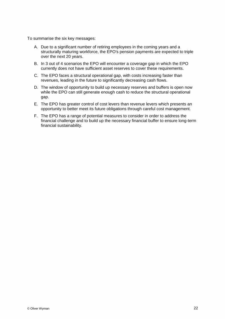
To summarise the six key messages:

A. Due to a significant number of retiring employees in the coming years and a structurally maturing workforce, the EPO's pension payments are expected to triple over the next 20 years.

B. In 3 out of 4 scenarios the EPO will encounter a coverage gap in which the EPO currently does not have sufficient asset reserves to cover these requirements.

C. The EPO faces a structural operational gap, with costs increasing faster than revenues, leading in the future to significantly decreasing cash flows.

D. The window of opportunity to build up necessary reserves and buffers is open now while the EPO can still generate enough cash to reduce the structural operational gap.

E. The EPO has greater control of cost levers than revenue levers which presents an opportunity to better meet its future obligations through careful cost management.

F. The EPO has a range of potential measures to consider in order to address the financial challenge and to build up the necessary financial buffer to ensure long-term financial sustainability.

© Oliver Wyman 23

1. Purpose and context of this document

1.1. Mandate and purpose of this document

It is the European Patent Office’s (EPO) responsibility towards its stakeholders to ensure financial sustainability at all times. Thus, the Office has mandated Mercer and Oliver Wyman to perform an independent assessment of the Office’s current financial situation and its evolution in the future. To fulfill this mandate, this Financial Study provides a view on a range of financial scenarios on an IFRS basis over a 20-year time horizon as well as an estimate as to whether the EPO can meet its financial obligations within each scenario. However, this document does not provide a view on or make any recommendations as to which actions the EPO management should take and decide to communicate to relevant stakeholders. All scenario results have been forecasted based on a proprietary financial model that has been built solely for this Financial Study. All underlying assumptions of the model and its functionality are described in section 3 of this report and have been discussed with and validated by key stakeholders across the EPO.

This study is for the exclusive use of the EPO. The opinions expressed in this study are valid only for the purpose stated herein and as at the date of this report. No obligation is assumed to revise this study to reflect changes in events or conditions which occur subsequently.

This study is not to be reproduced, quoted, modified, sold, distributed for any purpose or otherwise provided, in whole or in part, to any other person or entity without the prior written permission of Mercer and Oliver Wyman. There are no third-party beneficiaries with respect to this study, and neither Mercer nor Oliver Wyman accept any liability to any third party.

Information furnished by others, upon which all or portions of this study are based, is believed to be reliable but has not been independently verified, unless otherwise expressly indicated. Public information as well as industry and statistical data are from sources we deem to be reliable; as such, Mercer and Oliver Wyman make no representations or warranties as to the accuracy of the information presented and takes no responsibility or liability (including for indirect, consequential or incidental damages), for any error, omission or inaccuracy in the data supplied by any third party.

Mercer and Oliver Wyman have prepared the study for the EPO (together the “parties”) for the purpose of assisting the EPO in understanding any financial risks associated with its business as set out in the terms of an engagement letter between the parties dated 12 December 2018. Unless agreed otherwise in writing, Mercer and Oliver Wyman do not accept any liability or responsibility to any third party in respect of this study.

This study contains confidential and proprietary information of Mercer and Oliver Wyman and is intended for the exclusive use of the parties to whom it was provided by Mercer and Oliver Wyman.

The findings, ratings and/ or opinions contained in this study contain projections based on current data and historical trends. Any such projections are subject to inherent risks and uncertainties. Neither Mercer nor Oliver Wyman accept responsibility for actual results or future events. Past performance does not guarantee future results. All decisions in connection with the implementation or use of advice or recommendations contained in this study are the sole responsibility of the EPO. This study does not represent investment advice, nor does it provide an opinion regarding the fairness of any decision to any and all parties.

© Oliver Wyman 24

The remainder of this document explains the methodology, approach and assumptions that were applied, summarizes the key findings, describes the financial scenario analyzes that were conducted and their results as well as considerations and an outlook on potential managerial actions.

1.2. Previous Financial Studies and differences to the 2019 Financial Study

In 2010, an independent Financial Study was conducted, and issued on 21 January 2011, to review the EPO’s financial situation and to forecast its long-term financial sustainability. It simulated the long-term financial development in four scenarios and was the basis for subsequent reforms between 2011 and 2015 which were proposed by the EPO senior management and approved by the member states. A new Financial Study was performed in 2016 to assess the impact of the reforms and the evolution of the EPO’s long-term financial position.3 In 2010/-11, the scenario analysis reaffirmed certain structural challenges of the EPO, such as increasing total salary costs comprising basic salaries and social security costs, declining equity and liquidity and the potential need for additional funding. The 2016 Study had a focus on production and productivity and suggested a close monitoring of factors determining the financial situation. The study therefore recommended that the EPO should protect its financial performance achieved in 2011-2016 and prepare for the potential influences of external factors, such as the digitization of business models, and competing patent systems. Actions included, for example, the introduction of the EPOTIF and increasing productivity.

Some events – notably the continuation of a persistently low interest rate – could not fully be anticipated in 2016. In addition, pension schemes are maturing and are at a crossing point where contributions are beginning to be lower than the value of benefits paid annually. Furthermore, the treasury investment fund (EPOTIF) was introduced in 2018. Another change compared to the 2016 Financial Study are operational efficiency gains achieved in the past few years that have financial implications for the EPO. Together the impacts of the changed operational and macroeconomic situation of the EPO have made this Financial Study essential to provide the EPO management with the necessary information to address current challenges.4

This year’s Financial Study has three distinct characteristics compared to the Financial Studies conducted in 2010/-11 and 2016:

• Firstly, a proprietary financial model was built to forecast the financial statements over a 20-year horizon. As part of the scenario analysis, the results were reconciled with EPO internal bottom-up modelling whenever relevant. Explanations for remaining deviations were investigated if necessary.

• Secondly, the 2019 Financial Study includes an in-depth and comprehensive employee benefit modelling with the objective to ensure that future benefits can be paid out of available cash with an acceptable probability. The 2019 Financial Study uses detailed cash flows provided by the external actuarial provider to model changes in assumptions as well as changes to the employee benefits in greater detail. The benefit modelling also differs from the actuarial valuation conducted by the Actuarial Advisory Group (AAG). The AAG is tasked by the President every two

3 Please refer to CA/79/16 and the document “Independent Study of the Budgetary and Financial Strategy

of the European Patent Organization” as of 14/01/2011 for further details

4 Please refer to Invitation to tender No. 2912 Strategic Financial Consultancy Services

© Oliver Wyman 25

years to assess the level of future service contribution requirements for pensions, long-term care and healthcare only. Two of the major differences between the Actuarial Valuation and the 2019 Financial Study are that

1) the tax compensation liabilities are not in scope of their evaluation, and

2) assets are projected to grow with a constant rate without assuming capital market volatility.

The Financial Study accounts for past service to ensure the EPO can cover all benefit payments in the future including unfunded benefits (i.e., tax, family allowance and death). To support the prudent financial management of the EPO, the Financial Study allows for market volatility and time dependence of capital market returns.

• One recommendation of the 2016 Financial Study was the implementation of a more return-seeking liquidity reserve which the EPO introduced in 2018 (namely EPOTIF). The 2019 Financial Study allows for different performance of the EPOTIF based on capital market scenarios and strategic asset allocation. Similar performance modelling is also undertaken for the RFPSS, the Reserve Fund for Pensions and Social Security.

1.3. Approach

The Office has mandated Mercer and Oliver Wyman to perform an independent assessment of the Office’s current financial situation and its evolution in the future.

To evaluate the EPO’s long-term financial sustainability, Mercer and Oliver Wyman have developed a top-down approach.

The purpose of this approach is to provide a meaningful representation and analysis of the status quo and assessment of sensitivities to future macroeconomic developments. This Financial Study is intended as a basis for further discussion and to support development of alternatives for decision making by the EPO’s management and relevant stakeholders. It should not be considered as guidance towards specific recommendations or solutions.

The financial model developed during this study consists of two main parts:

Part One: Assessment of the EPO’s benefit obligations

The evaluation of the EPO’s benefit obligations is based on cash flow projections provided by the EPO’s actuary: International Service for Remunerations and Pensions (ISRP). The cash flow projections cover total benefits split by active and deferred employees as well as pensioners for the next 100 years as of 31/12/2017. For active employees, ISRP has also delivered accrued benefits such that future service costs for current actives can be deducted. It is important to note that the provided cash flow projections reflect a closed group meaning that the cash flows reflect the current population of active employees – therefore, new hires are modelled separately. To take new hires into account, Mercer’s actuaries have modelled future service costs assuming an average prototypical group of new hires. This allows modelling of the evolution of benefit obligations and additional contributions, dependent on assumed new hires. Main inputs for the model include the number of new hires in each year, economic parameters such as the relevant discount rate and demographic developments such as longevity.

© Oliver Wyman 26

Part Two: Forecasting of IFRS financial statements over a time horizon of 20 years, with a focus on the assessment of the EPO’s operational cash flow generation

The EPO’s operational cash flow generation was assessed by modelling a set of IFRS financial statements on a 20-year horizon from 2019 to 2038. In order to model the financial sustainability of the EPO, the 2019 Financial Study looks at the two financial figures “benefit funding gap” and “coverage gap/ surplus” by applying a real discount rate similar to the process followed by the Actuarial Advisory Group. The approach differs from that of the Actuarial Advisory Group as the discount rate reflects a higher probability of being achieved to ensure that the Office can meet benefit obligations to current and former employees with a higher degree of certainty. Therefore, the Financial Study requires a 66% probability of meeting the return target compared to a 40% probability assumed in the last Actuarial Valuation. The prudent discount rate yields a risk buffer of 23% compared to the approach in the last Actuarial Valuation. This approach, i.e. higher necessary funding, aims to build up a buffer in order to withstand capital market volatility and market drawdowns. The target return probability of 66% is defined such that it allows for capital market volatility but does not restrict the EPO severely in the allocation of operating cash surplus.

The benefit funding gap is a financial figure which shows the gap between benefit obligations (applying the prudent discount rate) and both RFPSS and EPOTIF in 2038. EPOTIF is taken into account as it was created to better manage cash and, subject to management decisions, could potentially be used to finance unfunded social liabilities in the future, i.e. OPS tax compensation, family allowance and death. EPOTIF currently serves as a buffer for future payments and no current cash outflows take place. The benefit funding gap reflects the economic burden the EPO faces beyond the 20-year projection horizon. In other words, the benefit funding gap reflects the additional required funding to be reserved for employee benefit payments. This is compared to the cash surplus, which is the accumulated operating cash flow the EPO earns over the next 20 years, to calculate the coverage gap/ surplus.

Cash flow is defined consistently across relevant accounting standards as “changes in cash and cash equivalents during a period. Cash comprises cash on hand and demand deposits. Cash equivalents are short-term, highly liquid investments that are readily convertible to known amounts of cash and which are subject to an insignificant risk of changes in value. Cash flows are inflows and outflows of cash and cash equivalents.”5

Both parts have been developed and assessed against the background of four financial scenarios (Optimistic, Base 1, Base 2, Stress scenario, see section 3.2) consisting of specified sets of differing external parameters determining the macroeconomic environment in which the EPO operates.

5 Definition of IAS 7 Statement of Cash Flows

© Oliver Wyman 27

2. Financial and operational status quo

2.1. Revenue

At the EPO, three pillars of revenue streams can be differentiated:

• Revenue from procedural fees (without internal renewal fees)

• Revenue from internal renewal fees

• Revenue from national renewal fees

Revenue from procedural fees is driven by fees paid in relation to certain steps of the Patent Grant Process (‘PGP’) such as filing, search, examination, opposition and appeal fees. They are defined by the EPO and paid in advance of each process step with the applicant being able to withdraw the application at any point of the PGP.

Internal renewal fees (‘IRF’) are paid to protect a pending application until the patent has been granted, refused or withdrawn. IRF are paid yearly from the beginning of the third year after filing of an application until the end of the opposition period. The EPO defines the value of IRF in each ordinal year (i.e. the age of an application since its date of filing).

National renewal fees (‘NRF’) are paid to protect the granted patent in the states where the applicant seeks protection. They are paid yearly from the end of the opposition period until the applicant decides to stop the patent protection. Individual member states define the value of NRF for each year of protection after the grant. The fees are currently split 50:50 between the member states and the EPO. The key drivers for NRF are the number of patents granted, the patents’ lifetime and the number of states in which the patents are protected.

Figure 13 depicts the EPO’s revenue development between 2008 and 2018. Notably, total IFRS revenue increased at 5.2% p.a. during this time period – from 1,211 MN€ in 2008 to 2,004 MN€ revenue in 2018. The largest year-by-year increases can be observed in 2009/-10 (11%) and 2014/-15 (8%) driven by productivity as well as fee increases.

Whilst revenue from procedural and national renewal fees grew consistently at approximately 5% p.a. between 2008 and 2018, revenue from internal renewal fees shows a negative trend from 2016 onwards. This was largely driven by an overall reduction of stock of search, examination and opposition cases (see Figure 22).

Growth in revenue from national renewal fees is due to an increase in patent demand as well as productivity and thus, Search, Examination and Opposition (SEO) production. Taken together, this leads to a growing number of patents in the ‘grant’ phase in which national renewal fees accrue.

Revenue from procedural fees is further broken down in Figure 14. During the time period under consideration, revenue from procedural fees increased by approximately 70% and grew 5.5% p.a. between 2008 and 2018 with fees from filings, search and examination accounting for the largest part of procedural revenues.

In general, all components of procedural revenue grew since 2008 with revenues from examination and opposition growing at higher rates than the other fee components (9.1% p.a. between 2008 and 2018). This increase was primarily driven by the EPO’s focus to reduce stock of examination cases.

© Oliver Wyman 28

Figure 13: Total revenues6 2008-20187; By revenue type, in MN€, CAGR 2008-2018

Source: EPO Financial Statements 2008–2017; EPO 2018 Annual report; Mercer and Oliver Wyman analysis

Figure 14: Revenue from procedural fees 2008-20187; By type of procedural fee, in MN€, CAGR 2008-2018


2.2. Total expenses

As depicted in Figure 15, total operating expenses steadily grew between 2008 and 2018 reaching a temporary high in 2015 with 1,948 MN€. Whilst they grew at 6.2% p.a. from 2008

6 Excluding other operating income and work performed and capitalized

7 2018 figures from EPO 2018 Annual report

1,500

1,000

0

500

2,500

2,000

588554 618

2016

327

543

509

2008 2011

330

335

350

810530

2009

38167

353

444 489

550

2010

63

1,654

20182

66

457

403

2015

471

69

578

76

2012

69

428

2013

71

446

520

2014

472

706

489

558

73 69

520545

2017

872767

548

1,2115051,413 1,454 1,518 1,573

1,794 1,888 1,933 2,004

1,272

5.4%

5.2%5.0%

Other Procedural FeeInternal Renewal FeesNRF

4.4%

5.2%

4.6%

5.5%

CAGR

’08-’18

900

0

450

94

258

68

342

588

2014

354

270

2008

68 63509

91

193

274

2009

76

618

2015

212

2010

72

222 218216

266

2011

279

2012

78

291

2013

225

310

8984

2016

265

550

352

182

320

356 362

2017

95

436

20181

810

530

872

554 578

7067672.9%

5.5%8.2%

3.3%

9.1%

2.9%

CAGR

’08-’18Other

Examination and Opposition

Filing and search

© Oliver Wyman 29

to 2013, they grew at a faster pace of 6.5% p.a. from 2013 onwards. However, since 2015 costs grew at a slightly slower pace again. Due to the knowledge-driven nature of PGP activities at the EPO (i.e. little machine/ production costs), employee benefit expenses make up the largest part of operating expenses (78% in 2008, 86% in 2018).

Figure 15: Total operating expenses 2008-20188, By expense type, in MN€, CAGR 2008-2018


Thus, the increase in operating expenses was primarily driven by increasing employee benefit expenses, which doubled between 2008 and 2018 (see Figure 16).


2,000

500

2,500

1,000

1,500

0

188

1,948

2013

54601,203

60

942

20172008

58

2009

1,879

186

1,095

47

2010

55

57

252

188

1,133

2011

193

1,150

2012

213

203

1,626

1,368

2014

52

63

212

2,223

223

1,408

54

1,9082011,672

1,342

2015

1,648

2016

46

1,268222

1,021

1,672

1,378 1,398

1,9082,149

20181

6.2%

6.3%6.5%

Depreciation Employee benefit expensesOther operating expenses

0.5%

2.3%

7.3%

CAGR

’08-’18

© Oliver Wyman 30

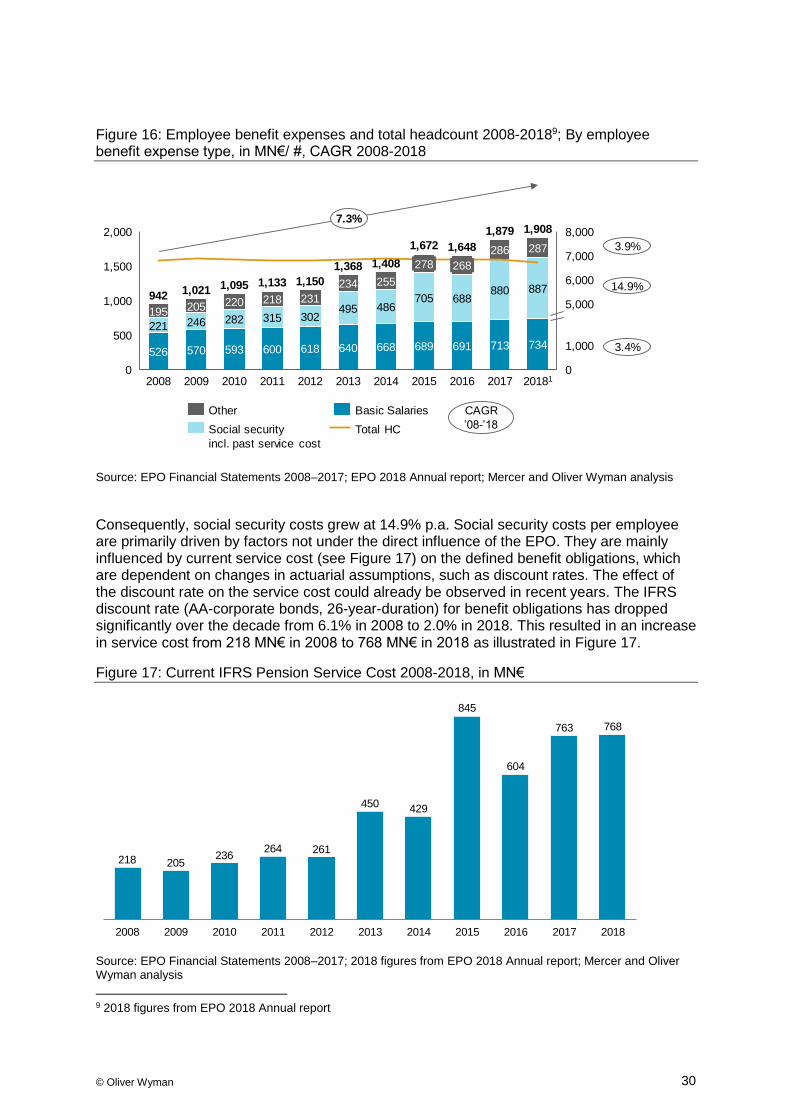
Figure 16: Employee benefit expenses and total headcount 2008-20189; By employee benefit expense type, in MN€/ #, CAGR 2008-2018


Consequently, social security costs grew at 14.9% p.a. Social security costs per employee are primarily driven by factors not under the direct influence of the EPO. They are mainly influenced by current service cost (see Figure 17) on the defined benefit obligations, which are dependent on changes in actuarial assumptions, such as discount rates. The effect of the discount rate on the service cost could already be observed in recent years. The IFRS discount rate (AA-corporate bonds, 26-year-duration) for benefit obligations has dropped significantly over the decade from 6.1% in 2008 to 2.0% in 2018. This resulted in an increase in service cost from 218 MN€ in 2008 to 768 MN€ in 2018 as illustrated in Figure 17.

Figure 17: Current IFRS Pension Service Cost 2008-2018, in MN€

Source: EPO Financial Statements 2008–2017; 2018 figures from EPO 2018 Annual report; Mercer and Oliver Wyman analysis


3.9%

14.9%

3.4%

CAGR

’08-’18

7,0001,500

1,000

8,000

00

1,000500

5,000

6,000

2,000

691

1,1331,095

2016 2017

195 302205

221

526

486

2008

246

268

570

2009

2201,021

282

287

593

2010

218

640

315

2013

231

618

234

2012

495

2014

255

713

278

668

705

2015

286

880 887

734

20181

600

942 688

1,408

1,672 1,6481,879 1,908

689

1,150

2011

1,368

7.3%

Other

Total HC

Basic Salaries

Social security

incl. past service cost

218 205236

264 261

450 429

845

604

763 768

20142008 20132009 201220112010 2015 2016 2017 2018

© Oliver Wyman 31

As the discount rate has a significant impact on the operating result, the EPO works internally with a standardized operating result by applying a constant discount rate of 5.0%. This makes the operating result comparable from year-to-year as the effect of a changing discount rate is eliminated by applying a constant discount rate of 5.0%.

Basic salary expenses primarily depend on the EPO’s total headcount, its distribution across job groups and salary adjustments due to inflation or career developments. They increased at 3.4% p.a. from 2008-2018 whilst overall headcount did not change significantly. However, the composition of headcount by job group shifted from JG 5-6 towards JG 1-4 in the observed period driving the overall increase of basic salary expenses together with salary increases due to factors including career progression and inflation-based adjustments.

Other employee benefit expenses comprise allowances, expenses for school and day-care centers, training activities, remuneration of other employees (e.g. interpreters) and other employee benefits not included in the above. They moved from 195 MN€ in 2008 to 287 MN€ in 2018, which was mainly driven by an increase of allowances and other benefits (e.g. expatriation, home leave, child care) from 142 MN€ in 2008 to 238 MN€ in 2018 in line with basic salary.

2.3. Total Equity

Figure 18 shows the development of equity between 2008 and 2018. Total equity declined from -1,787 MN€ in 2008 to -10,804 MN€ in 2018 driven by the low interest rate environment. The overall downward trend was largely driven by the remeasurement of defined benefit obligations as well as profit/ loss of the respective years.

Figure 18: Total Equity 2008-201810, in MN€



-4,000

-14,000

-12,000

-2,000

0

-10,000

-6,000

-8,000

2011

-10,867

2008 2009 2010

-1,787

2012 201620142013 2015 2017 2018

-4,585

-1,860 -1,833 -1,990

-5,143

-10,636

-12,340

-7,795

-10,804

© Oliver Wyman 32

2.4. Cash flow

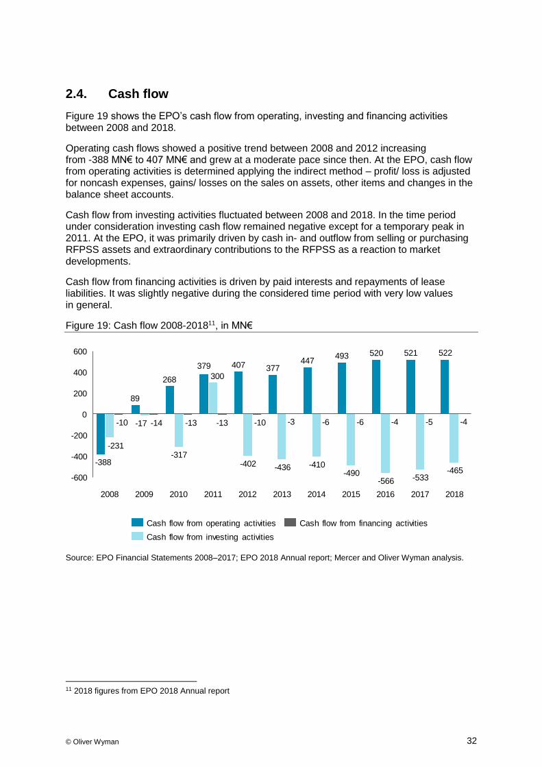
Figure 19 shows the EPO’s cash flow from operating, investing and financing activities between 2008 and 2018.

Operating cash flows showed a positive trend between 2008 and 2012 increasing from -388 MN€ to 407 MN€ and grew at a moderate pace since then. At the EPO, cash flow from operating activities is determined applying the indirect method – profit/ loss is adjusted for noncash expenses, gains/ losses on the sales on assets, other items and changes in the balance sheet accounts.

Cash flow from investing activities fluctuated between 2008 and 2018. In the time period under consideration investing cash flow remained negative except for a temporary peak in 2011. At the EPO, it was primarily driven by cash in- and outflow from selling or purchasing RFPSS assets and extraordinary contributions to the RFPSS as a reaction to market developments.

Cash flow from financing activities is driven by paid interests and repayments of lease liabilities. It was slightly negative during the considered time period with very low values in general.

Figure 19: Cash flow 2008-201811, in MN€

Source: EPO Financial Statements 2008–2017; EPO 2018 Annual report; Mercer and Oliver Wyman analysis.


400

-200

0

-600

200

-400

600

2015

520

-13

407

2009

-566

268

20122008 2010 2011 2013 2014 2016 2017

-13

-231

-388

-10

89

-17 -4-14

-317

377379

-6

300

-402

521

-10

2018

-436

-3

-410

-4-6

447

-490-533

522

-5

-465

493

Cash flow from operating activities

Cash flow from investing activities

Cash flow from financing activities

© Oliver Wyman 33

2.5. Productivity, SEO Production and stock

At the EPO, Products per Head (PpH) is a key measure of productivity.

As illustrated in Figure 20, PpH showed a 4.5% change from 2008 to 2014. 2014 marks a paradigm shift at the EPO - from 2014 onwards, stock was significantly reduced by a productivity boost following a management decision to increase efforts to meet Early Certainty criteria. Productivity increased from 76.5 PpH in 2014 to 99.8 PpH in 2018 following this shift. Growth was primarily due to increased Search, Examination and Opposition (SEO) production time per examiner and faster processing of products in general.

Production refers to the examiners’ activity associated with each step of the PGP, primarily search, examination and opposition of patent applications. The PpH changes were partly driven by the findings of the previous financial studies and subsequent initiatives, such as the introduction of productivity-related KPIs and performance-related pay.

Figure 20: PpH development 2008-2018

Source: EPO Management Dashboard 2008–2018; Mercer and Oliver Wyman analysis

Growing productivity from 2014 onwards and a subsequent increase in total SEO time led to a rapid increase of SEO production over the same time period (6.8% p.a. from 2014-2018) which exceeded growth in earlier years (0.7% p.a. from 2008-2014), as shown in Figure 21. This was additionally reinforced by a growing number of applications.

Due to the EPO’s focus on processing examinations, high growth rates in PpH between 2014 and 2018 were primarily driven by steep increases in examination/ opposition production growing at 16.5% p.a. Production of search cases grew at 2.3% p.a. over the same time period. By increasing PpH and SEO production, the EPO managed to increase its revenue at a fast pace from 2014 onwards (see Figure 21).

20142013

76.9

2008 20102009 2011 20152012 2016 2017 2018

73.2 76.1 78.4 78.8 78.4 76.5

86.592.9 95.5

99.80.7%

6.8%

CAGRPpH development

© Oliver Wyman 34

Figure 21: SEO production 2008-2018, total products, in K, CAGR 2008-2018


Figure 22: SEO stock 2008-2018, total products, in K, CAGR 2008-2018


The increase in SEO production from 2014 onwards significantly influenced the number of cases in EPO’s stock. With the introduction of the Early Certainty Initiative in the second half of 2014, the EPO set itself the goal to conduct searches on average within 6 months after filing and examinations on average within 12 months after examination request. Consequently, the EPO grew its production (see Figure 21), which led to a steady decrease in pending search cases from 183 K cases in 2014 to 102 K cases in 2018. In 2016, the reduction of stock began to materialize on the examination side as well. Pending examination cases decreased from 607 K cases in 2016 to 562 K cases in 2018. In total, the increase in examiner productivity and the focus on in-time processing of search and examination cases led to a decrease of stock by 14.6% from 2014 to 2018.

100

0

200

500

300

400

299

107

233

100

174

2008

109

190

2009 2017

115

2013

190

116

2010

203

116

195

365

245

2011

198

127

2012

112

167

213

2014 2015

151

2016

197

2018

430396

311

248238

274305 320316313

4142.9%

4.6%6.4%

Examination/Opposition Search

7.0%

3.0%

CAGR

’08-’18

0

800

200

400

600

729

2012 2017

188196

2008

503607

188

594517

129

2009

664696

194

705

522 541

2011

194102

559

192

574

183

777

2014

765

159

736

618

2016

592

104

562

201820152010 2013

777698 716 753

1.8%

-0.5%

-2.8%

-6.3%

1.1%

CAGR

’08-’18Search Examination/Opposition

© Oliver Wyman 35

3. Approach and scenario assumptions

3.1. Methodological approach

The key objective of the 2019 Financial Study is to model the EPO’s financial position over a time horizon of 20 years and to evaluate how strategic initiatives influence this financial position12. To demonstrate how exogeneous factors as well as internal development interact and impact the EPO, the financial model is divided in two main parts:

• Part one consists of the assessment of the EPO’s benefit obligations

• Part two consists of a forecasting of the IFRS financial statements over a time horizon of 20 years, with a focus on the assessment of the EPO’s operational cash flow generation

Both parts have been developed and assessed against the background of four financial scenarios consisting of sets of differing external parameters determining the macroeconomic environment in which the EPO operates.

While Mercer and Oliver Wyman developed their own approach and assumptions for this Financial Study, the Study always uses available data from the EPO. Where possible, reconciliation and alignment with EPO assumptions were ensured. Additionally, the Financial Study leverages data and forecasts for parameter development from relevant and accepted institutions providing benchmarks, e.g. the European Central Bank, the OECD and others. The applied approach as well as the scenario parameters are guided by established and proven principles employed by international organizations.

3.2. Introduction of four scenarios

Forecasting a 20-year development of the EPO’s financial position is inevitably a very uncertain exercise, as these positions will be impacted by factors which cannot be predicted with certainty.

Therefore, four scenarios were developed (an Optimistic, Base 1, Base 2 and Stress scenario) defined by a set of external factors (which cannot be influenced by the EPO) that determine the economic environment in which the organization operates. The scenarios represent possible evolutions of the future and illustrate how the Office’s financial situation may differ in more and less favourable economic circumstances. By no means should these scenarios be understood as the only ways in which the Office’s future situation may evolve. The span established by the different scenarios provides an indicative range which is considered appropriate to assess the impact of potential managerial actions on the longer-term sustainability of the EPO’s overall financial position.

12 Invitation to tender No. 2912 Strategic Financial Consultancy Services

© Oliver Wyman 36

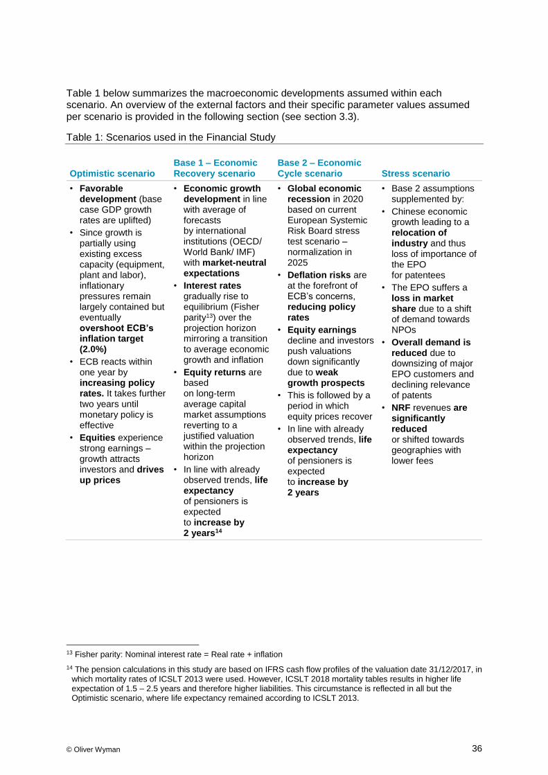
Table 1 below summarizes the macroeconomic developments assumed within each scenario. An overview of the external factors and their specific parameter values assumed per scenario is provided in the following section (see section 3.3).

Table 1: Scenarios used in the Financial Study

Optimistic scenario Base 1 – Economic Recovery scenario

Base 2 – Economic Cycle scenario Stress scenario

• Favorable development (base case GDP growth rates are uplifted)

• Since growth is partially using existing excess capacity (equipment, plant and labor), inflationary pressures remain largely contained but eventually overshoot ECB’s inflation target (2.0%)

• ECB reacts within one year by increasing policy rates. It takes further two years until monetary policy is effective

• Equities experience strong earnings – growth attracts investors and drives up prices

• Economic growth development in line with average of forecasts by international institutions (OECD/ World Bank/ IMF) with market-neutral expectations

• Interest rates gradually rise to equilibrium (Fisher parity13) over the projection horizon mirroring a transition to average economic growth and inflation

• Equity returns are based on long-term average capital market assumptions reverting to a justified valuation within the projection horizon

• In line with already observed trends, life expectancy of pensioners is expected to increase by 2 years14

• Global economic recession in 2020 based on current European Systemic Risk Board stress test scenario – normalization in 2025

• Deflation risks are at the forefront of ECB’s concerns, reducing policy rates

• Equity earnings decline and investors push valuations down significantly due to weak growth prospects

• This is followed by a period in which equity prices recover

• In line with already observed trends, life expectancy of pensioners is expected to increase by 2 years

• Base 2 assumptions supplemented by:

• Chinese economic growth leading to a relocation of industry and thus loss of importance of the EPO for patentees

• The EPO suffers a loss in market share due to a shift of demand towards NPOs

• Overall demand is reduced due to downsizing of major EPO customers and declining relevance of patents

• NRF revenues are significantly reduced or shifted towards geographies with lower fees

13 Fisher parity: Nominal interest rate = Real rate + inflation

14 The pension calculations in this study are based on IFRS cash flow profiles of the valuation date 31/12/2017, in which mortality rates of ICSLT 2013 were used. However, ICSLT 2018 mortality tables results in higher life expectation of 1.5 – 2.5 years and therefore higher liabilities. This circumstance is reflected in all but the Optimistic scenario, where life expectancy remained according to ICSLT 2013.

© Oliver Wyman 37

3.3. Identification of external parameters defining the four scenarios

The EPO’s financial situation partly depends on external parameters shaping the macroeconomic environment the EPO operates in. Potential external parameters have been identified by applying the PESTEL framework:

• Political drivers (e.g. trade conflicts, Brexit, foreign political climate)

• Economic drivers (e.g. capital market returns, inflation, credit conditions, R&D expenditures, GDP growth, interest rate)

• Sociocultural drivers (e.g. longevity, workforce availability)

• Technological drivers (e.g. impact of digitization and Artificial Intelligence)

• Environmental drivers (e.g. climate change and ecosystem at risk)

• Legal drivers (e.g. Unitary Patent, European Patent Convention and competition with other patent offices)

3.4. External parameter values

Each identified external parameter resulting from the PESTEL framework was analyzed and prioritized by the expected financial impact on the key components of the EPO’s financial statements. Table 2 provides an overview of the shortlisted parameters, their relevance assessment as well as the assumed parameter values per scenario applied in the financial model.

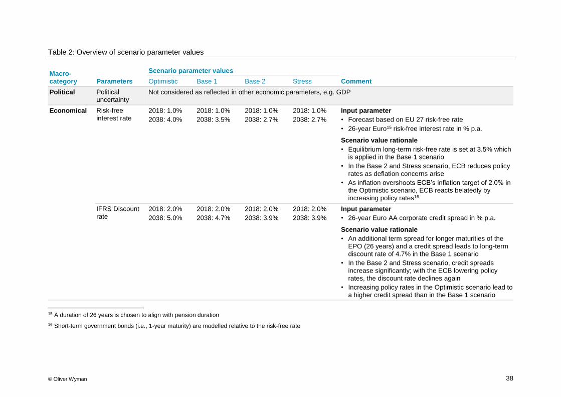
© Oliver Wyman 38

Table 2: Overview of scenario parameter values

Macro- category Parameters

Scenario parameter values

Comment Optimistic Base 1 Base 2 Stress

Political Political uncertainty

Not considered as reflected in other economic parameters, e.g. GDP

Economical Risk-free interest rate

2018: 1.0%

2038: 4.0%

2018: 1.0%

2038: 3.5%

2018: 1.0%

2038: 2.7%

2018: 1.0%

2038: 2.7%

Input parameter • Forecast based on EU 27 risk-free rate

• 26-year Euro15 risk-free interest rate in % p.a.

Scenario value rationale • Equilibrium long-term risk-free rate is set at 3.5% which

is applied in the Base 1 scenario

• In the Base 2 and Stress scenario, ECB reduces policy rates as deflation concerns arise

• As inflation overshoots ECB’s inflation target of 2.0% in the Optimistic scenario, ECB reacts belatedly by increasing policy rates16

IFRS Discount rate

2018: 2.0%

2038: 5.0%

2018: 2.0%

2038: 4.7%

2018: 2.0%

2038: 3.9%

2018: 2.0%

2038: 3.9%

Input parameter • 26-year Euro AA corporate credit spread in % p.a.

Scenario value rationale • An additional term spread for longer maturities of the

EPO (26 years) and a credit spread leads to long-term discount rate of 4.7% in the Base 1 scenario

• In the Base 2 and Stress scenario, credit spreads increase significantly; with the ECB lowering policy rates, the discount rate declines again

• Increasing policy rates in the Optimistic scenario lead to a higher credit spread than in the Base 1 scenario

15 A duration of 26 years is chosen to align with pension duration

16 Short-term government bonds (i.e., 1-year maturity) are modelled relative to the risk-free rate

© Oliver Wyman 39




Price index (Inflation rate)

2018: 100

2038: 149

Average over 20 years: 2.0%

2018: 100

2038: 140


2018: 100

2038: 128


2018: 100

2038: 128


Input parameter • Eurozone inflation in % p.a.

Scenario value rationale • In the Base 1 scenario, YoY Eurozone inflation is

the market-implied forward curve17

• Due to global growth below expectation, there is deflation after crisis (i.e. 2021 – 2022) in the Base 2 and Stress scenario

• In the Optimistic scenario, growth is partially using existing excess capacity such that inflation overshoots ECB’s inflation target

European Equity market index

2018: 100

2038: 381

2018: 100

2038: 325

2018: 100

2038: 205

2018: 100

2038: 205

Input parameter • Returns in % p.a.

Scenario value rationale • Growth-dividend-discount model: The model is a

build-up model which determines the long-term expected return by the current dividend yield, long-term expected earnings growth, P/E adjustment and inflation.

• In the Base 2 and Stress scenario, equities drop by 30% in year 2021 with a recovery in the following three years

• In the Optimistic scenario, the expected return for equities is 1% higher (i.e. 7.4%) than in the Base 1 scenario (refer to 3.4.4 for details)

17 Source: Barclays

© Oliver Wyman 40




Credit spread 2018: 1.0%

2038: 1.0%

2018: 1.0%

2038: 1.2%

2018: 1.0%

2038: 1.2%

2018: 1.0%

2038: 1.2%

Input parameter • 26-year Euro AA corporate credit spread in % p.a.18

Scenario value rationale • The Base 1 scenario builds on the mean scenario of

the Cox-Ingersoll-Ross model

• In the Optimistic scenario, with the economy being in good conditions, the credit spread stays 20bps below the Base 1 scenario assumptions

• In the Base 2 and Stress scenario, credit spreads increase significantly; with the ECB lowering policy rates, the discount rate declines again

Salary development

Considered for assessment of salary policy

R&D expenditure

R&D projection linked to GDP growth Input parameter • Real GDP growth in %

• Projection linked to GDP growth

• Assumed that the R&D to GDP ratio stays at its current level and the R&D stock growth follows R&D expenditure growth and is in effect linked to GDP growth

• China and Korea are an exception to this rule of stability. It is expected that China will follow the Korean example of government-driven investment into R&D to promote China as a global driver of innovation. In the Base 1 scenario, it is assumed that the Chinese R&D-to-GDP ratio will catch up to the current Korean R&D-to-GDP ratio, leading to a further increase in China ‘s R&D stock over the next 20 years

18 26-years to align with pension duration

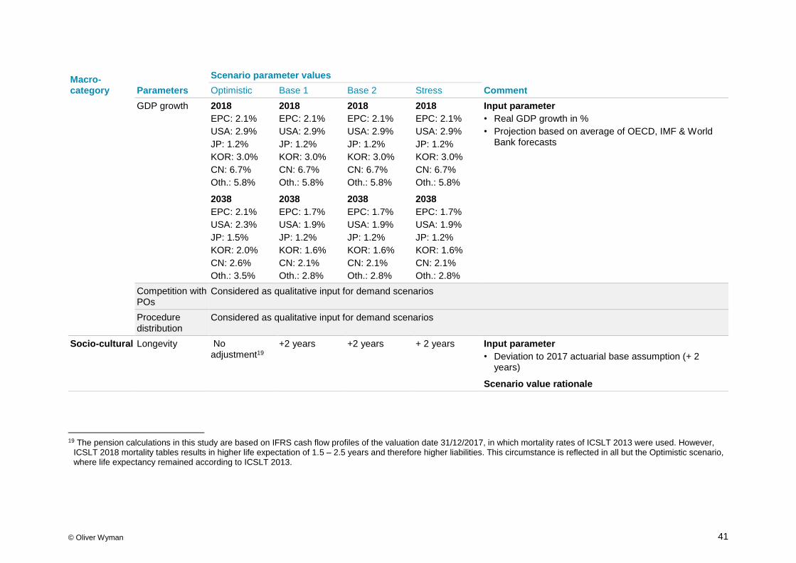
© Oliver Wyman 41




GDP growth 2018 EPC: 2.1%

USA: 2.9%

JP: 1.2%

KOR: 3.0%

CN: 6.7%

Oth.: 5.8%

2038 EPC: 2.1%

USA: 2.3%

JP: 1.5%

KOR: 2.0%

CN: 2.6%

Oth.: 3.5%

2018 EPC: 2.1%

USA: 2.9%

JP: 1.2%

KOR: 3.0%

CN: 6.7%

Oth.: 5.8%

2038 EPC: 1.7%

USA: 1.9%

JP: 1.2%

KOR: 1.6%

CN: 2.1%

Oth.: 2.8%

2018 EPC: 2.1%

USA: 2.9%

JP: 1.2%

KOR: 3.0%

CN: 6.7%

Oth.: 5.8%

2038 EPC: 1.7%

USA: 1.9%

JP: 1.2%

KOR: 1.6%

CN: 2.1%

Oth.: 2.8%

2018 EPC: 2.1%

USA: 2.9%

JP: 1.2%

KOR: 3.0%

CN: 6.7%

Oth.: 5.8%

2038 EPC: 1.7%

USA: 1.9%

JP: 1.2%

KOR: 1.6%

CN: 2.1%

Oth.: 2.8%

Input parameter • Real GDP growth in %

• Projection based on average of OECD, IMF & World Bank forecasts

Competition with POs

Considered as qualitative input for demand scenarios

Procedure distribution

Considered as qualitative input for demand scenarios

Socio-cultural Longevity No adjustment19

+2 years +2 years + 2 years Input parameter • Deviation to 2017 actuarial base assumption (+ 2

years)

Scenario value rationale

19 The pension calculations in this study are based on IFRS cash flow profiles of the valuation date 31/12/2017, in which mortality rates of ICSLT 2013 were used. However,

ICSLT 2018 mortality tables results in higher life expectation of 1.5 – 2.5 years and therefore higher liabilities. This circumstance is reflected in all but the Optimistic scenario, where life expectancy remained according to ICSLT 2013.

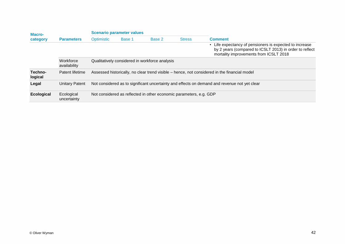
© Oliver Wyman 42




• Life expectancy of pensioners is expected to increase by 2 years (compared to ICSLT 2013) in order to reflect mortality improvements from ICSLT 2018

Workforce availability

Qualitatively considered in workforce analysis

Techno-logical

Patent lifetime Assessed historically, no clear trend visible – hence, not considered in the financial model

Legal Unitary Patent Not considered as to significant uncertainty and effects on demand and revenue not yet clear

Ecological Ecological uncertainty

Not considered as reflected in other economic parameters, e.g. GDP

© Oliver Wyman 43

3.4.1. Deep-Dive: Risk-free interest rate

Risk-free interest rate is an outcome of Mercer’s stochastic capital market scenarios. The Optimistic, Base 1 and Base 2/ Stress scenarios (with the latter two having the same risk-free interest rate) are representative paths derived from this model (see Figure 23).

In the Base 1 scenario, risk-free rate (10-year duration) is based on the mean scenario of the Hull & White 2-factor model20 and Fisher parity: Nominal rate = Real rate + inflation = 3.5% (rate to be reached in the long-term). Interest rates gradually rise to equilibrium (Fisher parity21) over the projected horizon mirroring a transition to average economic growth and inflation. The Fisher parity states that the nominal interest rate is equal to the real interest rate and inflation. Applying the Fisher parity, the equilibrium long-term risk-free rate is set at 3.5% where the individual components of the derivation are:

• Forward-looking inflation: 2.0% (“The ECB aims at inflation rates of below, but close to, 2% over the medium-term.”)22

• Real rate: 1.5% (Over the last 20 years, the average GDP growth rate has been 1.5% for the Eurozone)23

Please note that the Fisher parity only holds in the last year of the projection horizon, i.e. 2038. The other years mark transition years where the economy moves to equilibrium. In these years, real rates are lower while inflation is already at a level close to 2.0%.

In the Optimistic and Base 2/ Stress scenario, risk-free rate evolves in line with the Base 1 scenario over the first two years. In order to control overshooting inflation, ECB then increases short-term interest rates in the Optimistic scenario which also has the effect of increasing long-term interest rates. In the Base 2/ Stress scenario, risk-free rate drops to 0.0%. Interest rates increase only half as fast as in the Base 1 scenario in the following years.

20 The Hull-White Interest Rate model is a common model in the family of short rate models. In its two-factor

form, it models the respective interest rate curve using two stochastic processes and allows real and nominal interest rates as well as the development of inflation to be modelled simultaneously. Mercer uses a Hull & White 2-factor model to simulate the nominal and real yield curve.

21 Source: Fisher, Irving (1977): The Theory of Interest; Porcupine Press.

22 Source: https://www.ecb.europa.eu/mopo/html/index.en.html

23 Source: OECD

© Oliver Wyman 44

Figure 23: Risk-free rate, 10 years, in %


3.4.2. Deep-Dive: Discount rate

Discount rate is the rate which is used to determine present values of future payments such as pension payments. Since pension payments have a long duration the discount rate has a strong effect on the analysis performed in this financial study – a higher discount rate leads to lower present values of pension payments and vice versa.

AA corporate discount rate is an outcome of Mercer’s stochastic capital market scenarios with AA corporate discount rate (nominal, 26-year duration) = Risk-free rate + AA credit spread + term spread. The Optimistic, Base 1 and Base 2/ Stress scenarios are representative paths derived from this model (see Figure 24).

In the Base 2/ Stress scenario, credit spreads increase significantly within the first years – with the ECB lowering policy rates, the discount rate declines again. In the Optimistic scenario, increasing policy rates lead to a higher credit spread than in the Base 1 scenario.

Figure 24: AA discount rate, 26 years, in %


3.5%

4.0%

2.7%

1.0%

203020282018 2020 2022 20262024 2032 2034 2036 20380 %

1 %

2 %

3 %

4 %

5 %

Optimistic Base 1 Base 2/Stress

4.7%5.0%

3.9%

20222020 20382018 2024 20322026 20342028 2030 20360%

1%

2%

3%

4%

5%

6%


© Oliver Wyman 45

3.4.3. Deep-Dive: Inflation

Valuation inflation is an outcome of Mercer’s stochastic capital market scenarios. The Optimistic, Base 1 and Base 2/ Stress scenario are representative paths derived from this model.

In the Base 1 scenario, valuation inflation (26 year duration) is a scenario of the Hull & White 2-factor model24. The 10-year inflation will move to ECB‘s inflation target of 2.0% in the medium-term. Additionally, there is a term spread for the 26 years Eurozone breakeven swap rate.

In the Optimistic scenario, quantitative easing allows inflation rates to increase. The ECB needs to react to an inflation rate above the inflation target of 2.0% within one year by increasing policy rates. The transition process takes further two years until the monetary policy is effective and interest rates are restored to a normal level.

In the Base 2/ Stress scenario, a market crisis in 2020 leads to deflation. Deflation risks are at the forefront of ECB’s concerns, so the ECB needs to reduce policy rates as a consequence. At the same time, credit spreads increase leading to a strong increase in the IFRS discount rate and strong DBO remeasurement effects. After the crisis, the interest rates and credit spreads normalize again.

This translates into the price index depicted in Figure 25.

Figure 25: Price index (inflation), base year = 2018


24 The Hull-White Interest Rate model is a common model in the family of short rate models. In its two-factor form, it models the respective interest rate curve using two stochastic processes and allows real and nominal interest rates as well as the development of inflation to be modelled simultaneously. Mercer uses a Hull & White

2-factor model to simulate the nominal and real yield curve.

2018 2020 2026

130

2024

120

2022 2028 2030 2032 2034 2036 20380

110

140

150


137 (1.6% inflation p.a.)



© Oliver Wyman 46

3.4.4. Deep-Dive: Equity Market index

Equity returns are based on long-term average capital market assumptions reverting to a justified valuation within the projection horizon.

A fundamental approach25 is, in Mercer and Oliver Wyman’s view, best suited for modelling of expected stock returns as it is a neutral approach. The underlying economic principle of the approach is that the long-term expected return on equities is determined by the dividend yield, long-term expected earnings growth, price-earnings ratio (P/E) adjustment and inflation. The P/E adjustment assumes that equities can be over- or undervalued where the reference to fair valuation is the long-term average of the price-earnings ratio. As of 31/12/2018, the P/E of the MSCI Europe is above its historical average such that the P/E adjustment is negative. The following table shows the derivation of the expected return (in %) for European Equities denominated in EUR:

Dividend yield = 3.5%

P/E adjustment =-1.1%

Real earnings growth = 2.0%

Expected real return = 4.4%

Inflation = 2.0%

Expected return in EUR = 6.4%

Source: MSCI Europe, Mercer Analysis

In the Optimistic scenario, equities experience strong earnings – growth attracts investors and drives up prices. Instead of a real earnings growth of 2.0%, the earnings growth assumption is 3.0% yielding an expected return of 7.4% in the Optimistic scenario.

In the Base 2/ Stress scenario, equity earnings decline, and investors push valuations down significantly in the short run due to weak growth prospect. The market downturn is followed by a period in which equity prices recover. However, over the 20-year projection horizon the average equity return is 5.4%.

25 Fundamental analysis attempts to measure the intrinsic value by examining related economic and financial

factors, which can be both qualitative and quantitative in nature.

© Oliver Wyman 47

The assumed European equity market index is displayed in Figure 26.

Figure 26: European equity market index, base year = 2018, nominal


3.4.5. Deep Dive: Credit Spread

AA credit spread (26-year duration26) is an outcome of Mercer’s stochastic capital market scenario model (Cox-Ingersoll-Ross model27). The Optimistic, Base 1 and Base 2/ Stress scenarios are representative paths out of this stochastic model for the respective capital market environment.

In the Base 1 scenario, AA credit spreads increase over the long-term to 100bps. In the Optimistic scenario, the healthy condition of the economy leads to the credit spread staying

narrow, at 20bps below the Base 1 scenario assumption. In the Base 2/ Stress scenario,

spreads increase to 300bps in year 3 based on the tension in capital markets. This is followed by a normalization and from 2025 spreads stay at 100bps as in the Base 1

scenario.

3.4.6. Deep Dive: Mortality

A crucial assumption regarding the actuarial valuation of pension liabilities is mortality. Not only does mortality define the probability that an employee reaches his/ her retirement age and therefore receives pension payments, but it also provides the means to derive an expectation of how long a pension payment will last.

The cash flows that were used to assess the pension liability in this financial study stem from the actuarial valuation as of 31/12/2017, in which mortality rates according to International Civil Servants Life Table 2013 (ICSLT 2013) were used. The ICSLT 2013 contain a trend assumption for longevity, i.e. the later a person is born the higher the life expectancy.

26 The average duration of the EPO’s benefit liabilities is 26-years. Therefore, the scenarios are calibrated for

relevant AA credits spread with a duration of 26-years.

27 To ensure a consistent simulation of global corporate bonds using the interest rate model, Mercer uses the Cox-Ingersoll-Ross-model to simulate spreads across three currency regions: EUR, USD and GBP. The spreads are described analogous to the interest rate model by a stochastic mean reverting process.

100

202420202018 2022 2026 2028 2030 2032 2034 2036 2038

200

0

150

250

300

350

400

Optimistic Base 2/StressBase 1

325 (6.1% p.a.)

381 (6.9% p.a.)

205 (3.7% p.a.)

© Oliver Wyman 48

However, longevity is observed continuously and deviations from the trend assumption resulted in an updated version of the tables, ICSLT 2018, which provide a 1.5 – 2.5 years higher estimate for life expectancy. The cash flows used to assess the pension liabilities were adjusted in order to reflect the higher life expectancy in all but the Optimistic scenario.

3.5. Incoming Demand

3.5.1. Demand forecasting model

Based on the four scenarios and external parameters defined in section 3.4, incoming demand was forecasted over a 20-year time period by modelling the development of applications and new product orders (search). Empirical evidence shows that patenting demand is primarily driven by global economic activity, i.e. real (inflation-corrected) GDP and R&D28, which is why this link was used for these forecasts.

The dynamic distributed lag (DDL) model, which the EPO uses to forecast short-term demand development, was applied and tailored to the requirements of this study, i.e. long-term forecasting over a 20-year time period. It employs the concept of a “patent production function” and uses data from 2001 to 201729 to establish the following statistical relationship between growth in patent applications, real GDP and R&D stock developments, and past patent applications growth as explanatory variables:

Δ% 𝐴𝑝𝑝𝑠𝑡 ~ 0.579 × Δ% 𝐺𝐷𝑃𝑇𝑟𝑒𝑛𝑑 𝑡 + 0.679 × Δ% 𝐺𝐷𝑃𝐵𝑢𝑠𝑖𝑛𝑒𝑠𝑠 𝐶𝑦𝑐𝑙𝑒 𝑡 + 0.452 ×

Δ% 𝑅&𝐷𝑡 − 0.246 Δ% 𝐴𝑝𝑝𝑠𝑡−1 +0.081× Δ% 𝐴𝑝𝑝𝑠𝑡−2.

The model was adapted to the needs of a long-term demand development forecast by applying the following changes:

The model used by the EPO applies a constant for each of the 28 states. This constant is used to account for short-term heterogeneities in the demand growth which are not explained by the remaining factors of the patent production function. This is necessary as the patent production function does not contain a growth (or decline) factor unrelated to economic growth and R&D. These constants are not used for the projection in this study as the adapted model is used to make long-term projections into the future – projecting past, unexplained growth into the future might lead to an unrealistic diversion of growth between the states.

Furthermore, the model was not applied to all countries individually, but to the “IP5” blocks (EPC, US, Japan, Korea, China) and the block ‘Others’ for simplification.

3.5.2. Model inputs and results – Base 1: Economic Recovery scenario

The model inputs described in this section were applied to forecast growth of incoming demand in the Base 1 scenario. Additional assumptions made in the Optimistic, Base 2 and Stress scenario and any modifications are described in the following sections.

28 Such a relationship has been applied by e.g. Hingley, P., and W. G. Park, Do Business Cycles Affect

Patenting? Evidence from European Patent Office Filings, Technological Forecasting & Social Change 116 (2017) 76–86 or by de Rassenfosse and van Pottelsberghe de la Potterie, On the Price Elasticity of Demand for Patents, Oxford Bulletin of Economics and Statistics, Vol. 74, No. 1, p. 58-77.

29 Presented at the EPO Round Table on Forecasting 2019

© Oliver Wyman 49

Δ% GDP: The latest available real GDP growth forecast data for 2019 to 2038 as published by renowned international institutions30 was applied. If more than one source was available, the arithmetic average of the forecast was used.

Δ% R&D: For a majority of countries, the relationship between R&D and GDP has been very stable over the past two decades (see Figure 27) in the European Union, the US, Japan and India. Therefore, it is assumed that, in general, the R&D to GDP ratio stays at current levels and that R&D stock growth follows R&D expenditure growth and is, in effect, linked to GDP growth.

As Figure 27 shows, R&D-to-GDP ratio in China and Korea has increased in the past decade. It is expected that China will follow the Korean example of government-driven investment into R&D to promote China as a global driver of innovation. In the Base 1 scenario, it is therefore assumed that the Chinese R&D-to-GDP ratio will catch up to the current Korean R&D-to-GDP ratio, leading to a further increase in China ‘s R&D stock over the next 20 years.

Figure 27: R&D-to-GDP ratios, in %

Source: World Bank, World development Indicators, November 2018; NERA and Oliver Wyman analysis

Δ% Applications-1,t-2: The demand development forecasting also considers patterns over time measured by the EPO. These patterns account for the fact that annual spikes in demand are partially reversed in subsequent years, as the model adjusts to the long-run.

30 The IMF World Economic Outlook October 2018, World Bank Global Economic Prospects January 2019

and OECD Economic Outlook 103 and 104 databases 2018.

0,00

1,00

2,00

3,00

4,00

1996 1997 1998 1999 2000 2001 2002 2003 2004 2005 2006 2007 2008

European Union China India Japan Korea, Rep. United States

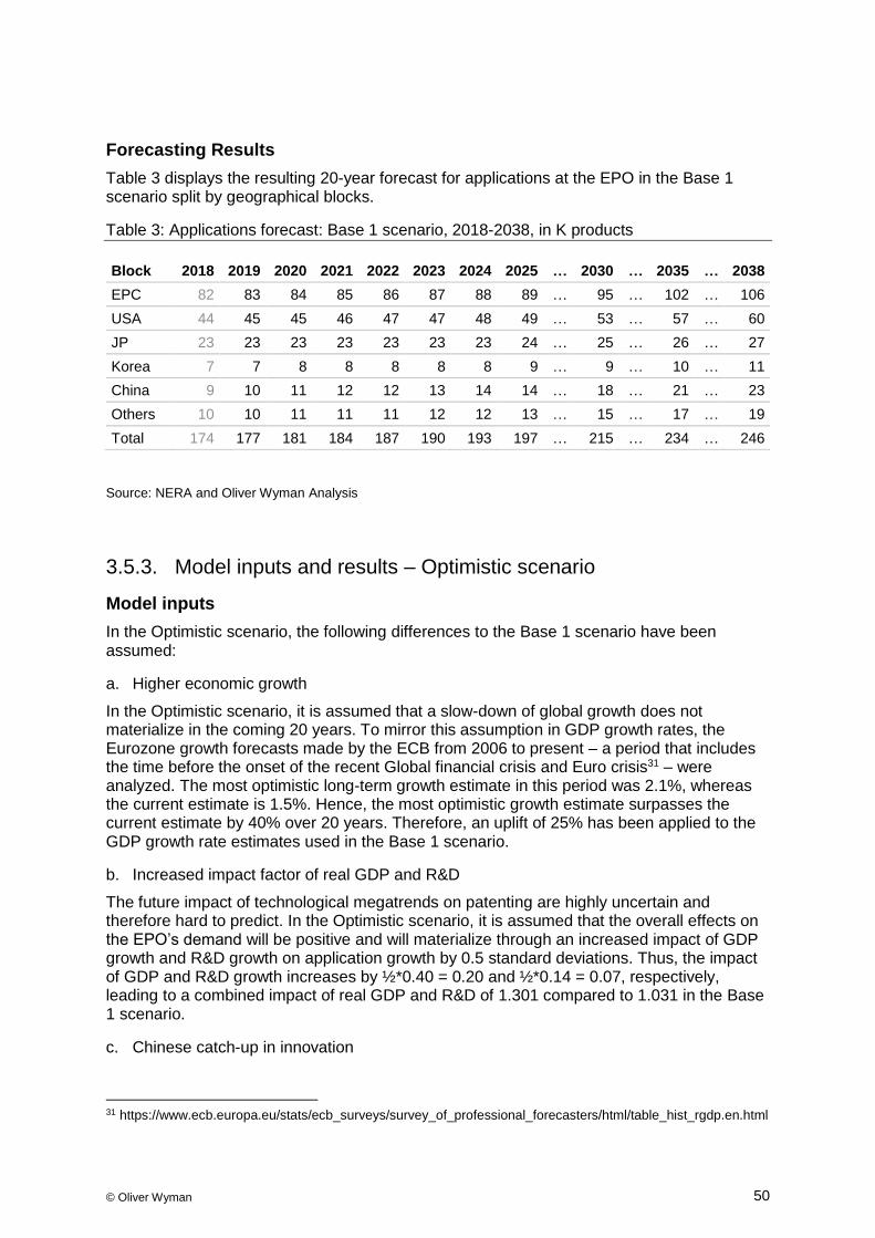
© Oliver Wyman 50

Forecasting Results

Table 3 displays the resulting 20-year forecast for applications at the EPO in the Base 1 scenario split by geographical blocks.

Table 3: Applications forecast: Base 1 scenario, 2018-2038, in K products

Block 2018 2019 2020 2021 2022 2023 2024 2025 … 2030 … 2035 … 2038

EPC 82 83 84 85 86 87 88 89 … 95 … 102 … 106

USA 44 45 45 46 47 47 48 49 … 53 … 57 … 60

JP 23 23 23 23 23 23 23 24 … 25 … 26 … 27

Korea 7 7 8 8 8 8 8 9 … 9 … 10 … 11

China 9 10 11 12 12 13 14 14 … 18 … 21 … 23

Others 10 10 11 11 11 12 12 13 … 15 … 17 … 19

Total 174 177 181 184 187 190 193 197 … 215 … 234 … 246

Source: NERA and Oliver Wyman Analysis

3.5.3. Model inputs and results – Optimistic scenario

Model inputs

In the Optimistic scenario, the following differences to the Base 1 scenario have been assumed:

a. Higher economic growth

In the Optimistic scenario, it is assumed that a slow-down of global growth does not materialize in the coming 20 years. To mirror this assumption in GDP growth rates, the Eurozone growth forecasts made by the ECB from 2006 to present – a period that includes the time before the onset of the recent Global financial crisis and Euro crisis31 – were analyzed. The most optimistic long-term growth estimate in this period was 2.1%, whereas the current estimate is 1.5%. Hence, the most optimistic growth estimate surpasses the current estimate by 40% over 20 years. Therefore, an uplift of 25% has been applied to the GDP growth rate estimates used in the Base 1 scenario.

b. Increased impact factor of real GDP and R&D

The future impact of technological megatrends on patenting are highly uncertain and therefore hard to predict. In the Optimistic scenario, it is assumed that the overall effects on the EPO’s demand will be positive and will materialize through an increased impact of GDP growth and R&D growth on application growth by 0.5 standard deviations. Thus, the impact of GDP and R&D growth increases by ½*0.40 = 0.20 and ½*0.14 = 0.07, respectively, leading to a combined impact of real GDP and R&D of 1.301 compared to 1.031 in the Base 1 scenario.

c. Chinese catch-up in innovation

31 https://www.ecb.europa.eu/stats/ecb_surveys/survey_of_professional_forecasters/html/table_hist_rgdp.en.html

© Oliver Wyman 51

Two distinct effects are considered:

Firstly, it is assumed that the catch-up of Chinese R&D activities to the Korean R&D-to-GDP ratio will be faster than in the Base 1 scenario. Convergence is assumed to be achieved within 10 rather than 20 years. When comparing the extent of Chinese applications at the EPO to its GDP, 1.04 applications are filed for every million US-$ of GDP which makes up only 34% of the US ratio32. This illustrates that, regarding international patent applications, China is still a relatively closed economy. In the Optimistic scenario, it is assumed that the new Chinese players on European markets will close this gap within 10 years.

Secondly, it is assumed that trade tensions evaporate leading to a surge in demand related to applications from China towards EPO services exceeding the expectations coming from forecasted GDP and R&D developments.

Forecasting results

Table 4 displays the resulting 20-year forecast for applications at the EPO in the Optimistic scenario split by geographical blocks.

Table 4: Applications forecast: Optimistic scenario, 2018-2038, in K products

Block 2018 2019 2020 2021 2022 2023 2024 2025 … 2030 … 2035 … 2038

EPC 82 84 85 87 88 90 91 93 … 103 … 115 … 124

USA 44 45 46 48 48 50 51 52 … 59 … 66 … 72

JP 23 23 23 23 23 24 24 24 … 26 … 29 … 30

Korea 7 7 8 8 8 9 9 9 … 11 … 13 … 14

China 9 13 16 20 25 30 36 42 … 71 … 85 … 93

Others 10 10 11 12 13 13 14 15 … 19 … 24 … 27

Total 174 182 190 198 206 215 225 236 … 289 … 332 … 359

NERA and Oliver Wyman Analysis

3.5.4. Model inputs and results – Base 2: Economic Cycle scenario

Model inputs

In the Base 2 scenario, the following differences to the Base 1 scenario have been assumed for the demand forecasting model inputs:

a. Adverse macroeconomic development

As described in section 3.2 the Base 2 scenario assumes a global economic recession in 2020 based on the current European Systemic Risk Board stress test, which leads to a global reduction in real GDP that only recovers slowly and normalizes in 2025.

b. Reduced impact factor of real GDP and R&D

The future impact of technological megatrends on patenting depends on a number of unknown factors. In the Base 2 scenario, it is assumed that the overall effects on the EPO’s demand will be negative and will materialize through a reduced impact of GDP growth and R&D growth on application growth by 0.5 standard deviations. The reasons for such a

32 The US can be considered as a benchmark to China as they both have a large internal domestic market

making them attractive for many inventors to protect their IP only locally

© Oliver Wyman 52

decoupling could either be of a legal nature33 or because other forms of IP protection become more applicable to inventions in digitization and AI. As a result, the impact of GDP and R&D growth decreases by ½×0.40=0.20 and ½×0.14=0.07, respectively, leading to a combined impact of real GDP and R&D of 0.761.

c. No Chinese catch-up in innovation

In the Base 2 scenario, it is assumed that the Chinese R&D-to-GDP ratio remains at current levels and does not increase further. Additionally, no other catch-up effects from China towards EPO patent demand are observed, given the underlying negative overall macroeconomic and trade environment.

Forecasting results

Table 5 displays the resulting 20-year forecast for applications at the EPO in the Base 2 scenario split by geographical blocks.

Table 5: Applications forecast: Base 2 scenario, 2018-2038, in K products

Block 2018 2019 2020 2021 2022 2023 2024 2025 … 2030 … 2035 … 2038

EPC 82 82 82 80 81 81 82 82 … 86 … 91 … 94

USA 44 44 44 43 43 43 44 44 … 47 … 50 … 51

JP 23 23 22 22 22 22 22 22 … 23 … 24 … 25

Korea 7 7 7 7 7 7 8 8 … 8 … 9 … 9

China 9 10 10 10 10 11 11 11 … 13 … 14 … 14

Others 10 10 10 10 10 11 11 11 … 13 … 14 … 15

Total 174 176 175 173 174 175 177 179 … 190 … 201 … 208


3.5.5. Model inputs and results – Stress scenario

Model inputs

As described in section 3.2, the Stress scenario is a modification of the Base 2 scenario. The following adaptations of the Base 2 scenario have been made:

Chinese economy growth

Given the shift of the world’s economic center of gravity towards China and the Asian-Pacific region and assuming an increasing regionalization of the global economy, it could be considered that Europe may be less of a key market for multinationals in the future. The Stress scenario is therefore based on the assumption that the share of applications from non-EPC member states declines, as the Chinese economy grows larger and at a stronger rate than the Eurozone, which proxies for the most significant market of the EPC. It is further assumed that this effect strengthens in the medium- and long-term, and that, from 2025 onwards, the EPO’s market share in global (i.e., also in the EPC) patenting further decreases by 0.75% p.a. through a shift to Asia.

33 Center for the Fourth Industrial Revolution „Artificial Intelligence Collides with Patent Law“ (2018).

© Oliver Wyman 53

Model results

Table 6 displays the resulting 20-year forecast for applications at the EPO in the Stress scenario split by geographical blocks.

Table 6 Applications forecast: Stress scenario, 2018-2038, in K products

Block 2018 2019 2020 2021 2022 2023 2024 2025 … 2030 … 2035 … 2038

EPC 82 82 82 80 81 81 82 82 … 83 … 83 … 84

USA 44 43 42 40 39 39 38 38 … 36 … 36 … 36

JP 23 22 21 20 20 20 19 19 … 18 … 17 … 17

Korea 7 7 7 7 7 7 7 7 … 6 … 6 … 6

China 9 9 9 9 9 9 10 10 … 10 … 10 … 10

Others 10 10 10 10 10 9 10 10 … 10 … 10 … 10

Total 174 173 170 166 166 165 165 165 … 163 … 163 … 164


3.5.6. Summary of incoming demand forecast

The consolidated forecast of the EPO’s application development between 2018 and 2038 is displayed in Figure 28.

Figure 28: Applications forecast across all scenarios, 2018-2038, in K products


2020 20302024 20262018 2022

200

2028 2032 20340

2036 2038

250

300

350

400

208174174

359

246

164

StressOptimistic Base 2Base 1

3.7%

1.7%

-0.3%

0.9%

CAGR

’18-’38

© Oliver Wyman 54

Observations of past developments have shown that long-term average growth rates of the EPO’s searches are almost identical to demand growth for patent applications. In the past, applications grew relatively consistently at approximately 0.1 percentage point p.a. faster than searches34. In the projections in this study, it is assumed that this difference remains constant year by year resulting in projections for new product orders (search) as displayed in Figure 29.

Figure 29: Search forecast across all scenarios, 2018-2038, in K products


3.6. Internal parameters of the Patent Grant Process

Part of the financial model developed during the 2019 Financial Study concerns the modelling of the Patent Grant Process (PGP). This requires certain assumptions regarding the development of internal operational parameters over the coming 20 years, which are outlined in this section. A detailed list of assumptions can be found in Appendix B.

3.6.1. Target Stock and timeliness

During the PGP, a certain number of cases at the EPO are said to be in stock, i.e. work on them has not yet started or it has started but has been paused. One of the main reasons for the stock is that the EPO grants the applicant certain time periods in which to reply or decide on the further processing of an application during which time the respective case is pending and remains in stock. Another potential reason for the buildup of stock is insufficient examiner capacity to process a case at a given point in time.

The EPO has an interest in ensuring timely processing of applications. This is, amongst other reasons, driven by the Early Certainty Initiative started on 1 July 2014 which is based on the objectives formulated at the Inter-Governmental Conference in Paris in 1999. Its aim is to ensure that applicants receive legal certainty regarding their application in a timely manner35.

Specifically, Early Certainty from Search requires that a search report accompanied by a written opinion is delivered within 6 months of the receipt of the file. At the 2018

34 EPO Landscape 2019, p.2.

35 cf. CA/97/16

2018 2024 20262020 2022 2028 2030

400

2032 2034 2036 2038 20400

200

300

500

238238

481

329

279

219

Base 1Optimistic Base 2 Stress CAGR

’18-’38

3.6%

1.6%

-0.4%

0.8%

© Oliver Wyman 55

yearly Round Table discussion, the target to reduce average search time even further to 5 months was presented36. Early Certainty from Examination aims at informing the public of an intended grant on average within 12 months of the examination request. Early Certainty from Opposition targets a final decision in standard opposition cases within on average 15 months of the opposition period’s expiry.

To determine target stock of pending cases in terms of output months as an input parameter for the financial model, these timeliness criteria need to be taken into consideration. To ensure a coherent definition of stock, the milestone concept was applied (see Figure 30). It clusters each product (i.e. Search, Examination, Opposition) into the milestones A to E as defined in the data warehouse user manual:

• Milestone A: Dossier is created

• Milestone B: Dossier is distributed for the first time to a productive unit

• Milestone C: End of the period of life of a dossier where final examiner action is expected

• Milestone D: End of the period of life of a dossier where final division action is expected

• Milestone E: Legal effect on the outcome of a product; dossier becomes historical

Figure 30: Overview over the milestone concept at the EPO

Source: Data Marts User Manual for Data Warehouse as of 10 July 2017

This concept illustrates the differentiation between the examiner and the case view on each product, e.g. examination. For the financial model, the case view is chosen as a basis as the IRFs payment period is determined on a case level. Therefore, target stock levels for search and examination are defined based on the case view as well.

Notably, to determine Search, Examination, Opposition production which is aligned with the EPO’s Medium-Term Business Plan assessment, a different view is applied than for the target stock definition. This is necessary as the case view includes periods of waiting times in which the examiner cannot work on the file. The two views are reconciled in the financial model37.

36 cf. MTBP 2019-2023 Planning process and DG 1 pending workload, Round Table 31 January 2018, p. 9.

37 Methodology: Total Search, Examination, Opposition production time is determined based on total examiner FTEs adjusted for non-SEO time e.g. training, sick leaves etc. Using the average days per product required to produce one search/ examination/ opposition, total SEO production is calculated. Adding the number of cases which are closed without production (e.g. due to withdrawal, non-payment of fees) results in the number of

© Oliver Wyman 56

As the standard timeline for searches does not include regular waiting times, a target stock level of 5 months is considered as a uniform target across all types of searches to align with the timeliness goal to finish search reports within an average of 5 months after filing. To define target examination stock, the Early Certainty criteria of 12 months is considered. However, when applying the case view, total time of cases in stock exceeds 12 months due to additional waiting times which are granted to the applicant throughout the process during which time the examiner cannot further process the case. These need to be included when taking the case view. The extent of these waiting times differs by type of examination (i.e. EP direct, E-PCT). Therefore, the regular examination timeline (including such waiting times) of each examination type was considered38 and a weighted average of the respective targets on a case level was calculated. This results in a target stock equivalent to 25 months for examination.

To ensure a “soft landing” at the respective target stocks for search and examination a stepwise reduction of stock as displayed in Figure 31 is assumed39.

Figure 31: Target stock search and examination development; pending cases in output months


3.6.2. Productivity

In the financial model examiner time per product is a key input metric for productivity on examiner level.

Time required per product is differentiated between SEO products. For 2018, times are defined as 1.98 days per search, 1.50 days per examination and 7.35 days per opposition on average40.

cases finished in the respective year – through this methodology, SEO production is transferred to the case view which is upheld throughout the entire financial model

38 Update on Early Certainty, March 2017, p. 27-28.

39 It should be noted that the reduction of stock is considered as a target, but its short-term achievement is subject to operational feasibility. In the Optimistic scenario examination target stock is achieved in 2027 due to production capacity limitations.

40 Source: EPO Finance, DG1, OW analysis; calibrated to total production figures in Management Dashboard 2018

5 5 5 5 5 5 5 5 5

34 3331

29 28 26 25 25 25

2018 2019 2020 202420222021 20252023 … 2038

Search Examination

© Oliver Wyman 57

Figure 32: Examiner time required per product, 2018–2038, in days, all scenarios


Across all scenarios, as of 2022 no further productivity improvements are expected without additional efforts, e.g. digitization. No such efforts are assumed in this study. Until 2022 a productivity increase of 3% is assumed that is reflected in the time required per search and examination respectively. This is expected to be mainly driven by efficiency improvements (i.e. incremental process improvements) and catching-up for sectors which currently experience time per product below average.

A drop in productivity is assumed between 2018 and 2020 due to planned investments such as the reduction of classification backlog which will naturally reduce SEO productivity41,42.

Another KPI used by the EPO to measure productivity is “Products per Examiner Head” (“PpH”), i.e. the total number of searches, examinations and oppositions (SEO) produced by the EPO divided by the number of examiners (man-years) in a given year.

As such it is influenced by additional factors43 on top of individual examiner performance:

1) Product mix: influence of search/ examination ratio

2) The proportion of examiner time spent on SEO activities vs. other activities such as classification time

3) Reduced productivity of new hires compared to experienced employees44

Until 2027 some volatility in PpH is assumed related to adjustments in S/E ratio and adjustments of workforce as well as investment in non-SEO activities. As of 2028 productivity is expected to reach a steady state across all scenarios as S/E ratios and the number of new hires are becoming stable in line with attainment of target stock and Early Certainty criteria – see section 3.6.1. The decrease of 3% in examiner time assumed in this study until 2022 has a positive effect on production per head. However, this effect is

41 As discussed during Round Table on Forecasting 2019 (“DG1 medium & long-term PGP strategy”)

42 While this will effectively reduce SEO time, in this study it is reflected in average time required per product

43 If not accounting for these factors (i.e. keeping them constant as of 2018) a 3% productivity increase as assumed in this study would result in 103 PpH as of 2022

44 Due to initial training and coaching requirements, new hires are assumed to only reach 53% and 71% of productivity in years 1 and 2, respectively. Afterwards, their productivity increases successively to 85% in year 3 and 92% in year 4

2018 2020 20322022 2024 2030

2.0

20282026 2034

0.5

2036 20380.0

1.0

1.5

2.5

1.50

1.98 1.92

1.45

Time/search Time/examination

© Oliver Wyman 58

overcompensated by opposing effects, such as changes in product mix and the proportion of examiner time spent on non-SEO activities. This leads to assumed PpH levels in 2038 between 92.0 and 92.8 for all scenarios. It should be noted that this does not include any additional efforts such as digitization.

Figure 33: Products per Head, 2018-2038, all scenarios


3.6.3. Workforce

Three groups of employees are considered separately in the financial model: examiners, formality officers and other employees. Employees within those job groups are then modelled by their Job Group and by their affiliation to OPS and NPS separately.

All employees are assumed to leave the EPO at the average retirement age of 61 years. No additional leavers are assumed during the time horizon of the study. Fixed-term contracts are assumed to be either replaced or made permanent.

For examiners, new hires are assumed to be in line with production requirements and hence driven by the number of employees retiring as well as incoming workload in the long-term. In terms of the financial model, the replacement ratio45 is determined such that the amount of pending cases is in line with the Early Certainty criteria described in section 3.6.1. Decreases in productivity due to training of newly hired examiners are considered in terms of the impact of initial training time on available SEO time.

New hires of formality officers are linked to the number of examiners, i.e. a constant ratio is assumed between examiners and formality officers.

For all other employees, a replacement ratio of 1 is assumed.

45 Replacement ratio is defined as number of new hires in a given period of time divided by employees leaving

the firm in the period

203420302018 2022

80

2026 2038

90

70

100

110

120

99.8

92.1

92.3

92.8

92.0

Optimistic Base 2Base 1 Stress

Steady stateConvergence phase

© Oliver Wyman 59

3.6.4. Production

Production in the financial model is modelled separately for search, examination and opposition for the 20 years covered by the Financial Study. For search and examination, a detailed approach is used for the projection of stock and production46. In this approach production, and as a result stock, is determined as a function of available workload, SEO time, productivity, target stock and minimum stock47.

Available workload is defined for each product as incoming workload plus stock available for production (total stock less minimum stock48). For search, incoming workload is explicitly modelled as described in section 3.5 based on macroeconomic indicators. Incoming workload for examination is projected based on the interpolation of historic patterns applied to the search production in a given year.

New hires and thus workforce are optimized annually to avoid temporary overcapacity whilst achieving target search and examination stock (as a second priority). No minimum replacement ratio is assumed. The ratio of search per examination (S/E ratio) is optimized together with the workforce with respect to the same target function.

Based on the workforce available for search, examination and opposition, SEO time is calculated49. Together with the time required for a product50 and the S/E ratio this determines the potential production possible with the workforce currently employed. Production is then determined as the minimum of available workload and potential production.

Other parameters relating to the PGP process, e.g. examinations leading to patents published, are forecasted based on interpolation of historical patterns. Details can be found in Appendix B.

3.7. Internal financial parameters

Financial statements are forecasted for 20 years until 2038 based on the IFRS accounting standard following the structure of the EPO’s IFRS financial statements as published for 2017. The methodology and key assumptions are outlined in this section. For a detailed list of assumptions refer to Appendix B.

3.7.1. Statement of Comprehensive Income

The main revenue streams and employee benefit expenses are forecasted based on the production and the workforce development as described in the previous section. Other operating expenses are assumed to grow with inflation. Positions with relatively small

46 Since opposition generates only a negligible share of revenue yearly opposition activities are assumed to be in

line with examination production

47 Production in the financial model is defined as searches, examinations and oppositions executed by examiners. Incoming and available workload and stock (pending cases) are considered in terms of cases in the EPO “Case view” – see section 3.6.1 for details. A factor as described in Appendix B is included to account for cases that are completed without production when these values are compared

48 Minimum stock is set to 5 months of potential search production output and 24 months of potential examination production output given the examiner workforce and time per product assumed in a given year in line with the long-term target stock under Early Certainty

49 See Appendix B for details

50 See section 3.6.2 for details

© Oliver Wyman 60

revenues and costs are assumed to grow in line with either revenue or basic salaries respectively.

Revenue from procedural fees related to the Patent Grant Process

The number of cases paying fees and the fee structure, which together determine revenue from procedural fees, are each modelled separately. The number of cases are forecasted based on the forecast of production figures as described in the previous section. Fees per product are forecasted based on historical income statements and production figures for individual line items, e.g. procedural fees for international searches - PCT. No fee increases other than a one-time increase of 4% in 2020 are assumed going forward.

Revenue from renewal fees for patent applications

Renewal fees for patent applications (Internal renewal fees, IRFs) are set depending on the age of the patent application (ordinal years) defined by the EPO. The two major drivers of revenue from internal renewal fees are the amount of cases paying fees and the age distribution of those cases.

In the financial model the number of cases currently paying internal renewal fees is modelled based on the number of pending cases (stock) for search and examination per ordinal year51,52.

The increased productivity of the EPO during the PGP has two effects on the revenues from IRFs: 1) the total number of cases paying IRFs decreases; and 2) those cases are younger on average. To reflect this shift in the foundation for IRFs in the financial model, an adjustment for changes in age structure is applied in addition to the effects caused by the decrease in fee paying cases.

With the assumed achievement of Early Certainty in 2024 it is expected that there are very few cases53 in the IRF stock older than 85 months54 (approximately 7.1 years). Hence, there is a cut-off (“cutting the tail”) of cases older than 7.1 years in the age distribution of IRF paying cases; this is assumed to happen gradually until completion in 2024.

National renewal fees

National renewal fees (NRFs) for granted patents are set depending on the age of the patent application (ordinal years) by the member states. The two major drivers of revenue from NRFs received by the EPO are the number of patents paying fees and the age distribution of those patents.

In the financial model NRFs are modeled on aggregate level (EPO grants), referred to as cases hereafter, not on the level of individual patents. The absolute number of cases currently paying national renewal fees is explicitly modelled per ordinal year. Newly granted patents enter this population with an age distribution linked to the age distribution of IRF cases and patents lapse with given maintenance rates. Maintenance rates are extrapolated to all member states based on the weighted average of those countries for which full data is

51 Ordinal year is defined as time since initial filing

52 The increase in divisional applications is implicitly considered in 2017/-18 figures

53 Some outliers older than 7.1 years are assumed to exist with a reduction of 80% compared to 2017 values

54 The maximum time from filing under Early Certainty is assumed to be 61 months for Euro-PCT, EPO not ISA, with/without PCT CHII allowing for an additional buffer of 24 months for divisionals; Opposition is neglected in this analysis;

© Oliver Wyman 61

available and are assumed to be constant over time in line with historical observations. The NRF fees structure is assumed to stay constant at current levels in this Financial Study.

The increased productivity of the EPO during the PGP has two effects on the revenues from NRFs: 1) the total number of cases paying NRFS increases with the number of patents granted; and 2) those cases are younger on average when they first pay national renewal fees. Hence, the same cut-off in the age distribution of newly granted patents entering the NRF stock is applied as to cases paying IRFs. The shift in the age distribution of newly granted patents then leads to a shift in the overall distribution of patents paying NRFs over time.

Employee benefit expenses

Current service cost (net of staff contributions), basic salaries of permanent employees, healthcare and other social security costs are forecasted using detailed modelling approaches. Oher employee benefit expenses are linked to basic salaries of permanent employees in this study.

Average salaries are assumed for employees within the job groups 1-4 and 5-6 respectively. A further distinction is made between employees in NPS and OPS.

For average salaries a yearly adjustment for career progression is assumed (1.74%) in addition to an adjustment for inflation (HICP + 0.5%).

The influence of new hires on average salaries is explicitly considered. Average entry level salaries are based on actuarial valuation and hence actual observation55 and adjusted for inflation up to 2038. Limitations of career progression in the salary grid are reflected in average salaries.

3.7.2. Statement of Financial Position

Changes in major positions are either directly linked to the statement of comprehensive income or forecasted using detailed modelling approaches, e.g. RFPSS, EPOTIF, DBOs, etc. not explicitly modeled positions are assumed to grow in line with revenue or basic salaries.

In the Financial Study, capital expenditure in property, plant and equipment of 14.6 MN€ p.a. is assumed. Additionally, 600 MN€ investment in buildings through to 2026 are considered56.

All excess cash flow is deposited into other financial assets and 1-year government bond interest rates are used as a proxy for the return generated by cash in short-term liquidity reserves (in contrast to for example assets in EPOTIF which are invested with a long-term focus).

55 See also Table 8

56 Source: Interview with PD General Administration (EPO) 18/02/2019; Mercer and Oliver Wyman analysis

© Oliver Wyman 62

3.7.3. Statement of Cash Flows

The statement of cash flows is calculated based on the statement of comprehensive income and statement of financial position.

For the projection of operating cash flow, the direct approach is chosen to better illustrate the key drivers of cash generated from the EPO’s operations. RFPSS and EPOTIF are considered to not be part of the EPO’s operations and are therefore treated as a separate entity for the purpose of determining operating cash flow. RFPSS is assumed to be activated, i.e. benefit payments of funded plans are financed by the assets of RFPSS. There are no contributions to and no payments from EPOTIF assumed.

Positions in the statement of cash flows related to cash receipts from customers are forecasted based on revenue and other operating income as calculated in the statement of comprehensive income adjusted for changes in pre-paid fees.

Positions related to cash paid to employees are forecasted based on employee benefit expenses as calculated in the statement of comprehensive income with the following adjustments57:

• Current service costs are excluded as they are non-cash transactions in the IFRS income statement

• Ordinary EPO contributions to RFPSS and SSP not explicitly considered in the IFRS income statement are included

• Adjustment for tax allowance, family allowance and death not explicitly considered in IFRS the income statement are included

Positions related to cash paid to suppliers are forecasted based on other operating expenses as calculated in the statement of comprehensive income with additional consideration of changes in assets and liabilities carried as working capital.

Positions related to investing activities are forecasted based on changes in the respective balance sheet items whereas cash flow from financing activities is assumed to be zero from 2019-2038. As no extraordinary contribution to either RFPSS or EPOTIF are assumed over the course of the study, there are no related transactions included in the cash flow from investing activities.

3.7.4. Pension modelling approach and assumptions

Modelling of long-term employee benefits

The EPO operates four plans treated as defined benefit obligations (DBOs) for its employees:

• Retirement pension plan including retirement for health reasons, a tax compensation and family allowances

• Long-term care insurance

• Health insurance

• Death and invalidity involving lump-sum payments.

57 An additional adjustment for non-cash items included in incomes statement items carried over in the cash flow

statement is made.

© Oliver Wyman 63

The long-term employee benefit schemes can be distinguished by their nature of being either funded or unfunded58:

Table 7: EPO employee-benefit schemes description

Funding status Scheme Main characteristics

Funded Pensions (OPS and NPS)

• OPS: Staff members joining prior to January 1st, 2009 (closed plan).

• NPS: Staff members joining after January 1st, 2009. Relevant scheme for new hires.

• 2% accrual rate per annum.

• 70% maximum accrual.

• Normal retirement age: 60.

• Salary cap:

– OPS: No salary cap.

– NPS: Twice G1/4 salary equivalent.

• Pensions fully indexed to salary inflation.

• Contribution rates depend on pensionable salary and are set by an independent Actuarial Advisory Group.

Long-term care (LTC)

• Compulsory insured beneficiaries are employees, former employees and their dependent children as well as orphans receiving a pension benefit from the pension plan.

• The benefit amount depends on the level of reliance of care and is a fixed percentage of the basic salary.

• Benefits are financed by regular contributions from the EPO (2/3rd) and employees (1/3rd of total contributions). Contribution rates depend on salary and are set by an independent Actuarial Advisory Group.

Health • An employee, who worked at the EPO until he/ she retires or who is in receipt of an invalidity benefit, his/ her spouse, his/ her children and other dependents are entitled to a reimbursement of medical costs.

• Benefits are financed by regular contributions from the EPO (2/3rd) and employees (1/3rd). Contribution rates depend either on salary or pension payments.

• Current total contribution rates (to RFPSS): Application of CA/D 7/10 to the basic salaries, pensions and invalidity allowances paid

• Contribution rates depend on pensionable salary and are set by an independent Actuarial Advisory Group.

Unfunded Tax allowance • Beneficiaries under the OPS only are entitled to a tax compensation that equals 50% of the theoretical amount by which the recipient’s pension needs to be topped up to take account of the reduction of pension due to national taxation.

58 For funded plans (OPS, NPS, LTC, Health) there is a dedicated reserve within the RFPSS. Unfunded plans are

paid by the EPO out of operatic cash. The EPOTIF can potentially be used to pay for these benefits in the future. Some marginal reserves for Tax allowance are made in the RFPSS and are allowed for in the financial study.

© Oliver Wyman 64

Funding status Scheme Main characteristics

• This tax compensation was previously reimbursed by the Member States in which taxes were paid. As from January 1st, 2009, tax compensation benefits are not reimbursed by the Member States to the Office’s budget anymore.

• For accounting purposes, the tax allowance liability is combined with the pension plan and shown as one plan on the balance sheet although this means in effect that a funded plan is mixed with two unfunded plans (i.e. tax and family allowance). Tax allowance is paid directly out of operating cash flow and not deducted from RFPSS.

Family allowance for pensioners

• The family allowance comprises household allowance, child and dependent's allowance, disabled child allowance, childcare allowance and education allowance.

• For accounting purposes, the family allowance liability is combined with the pension plan and shown as one plan on the balance sheet although this means in effect that a funded plan is mixed with two unfunded plans (i.e. tax and family allowance). Family allowance is paid directly out of operating cash flow and not deducted from RFPSS.

Death • The benefits payable is a fixed amount for funeral expenses incurred for the permanent employee himself/ herself, his/ her spouse and, where appropriate, his/ her dependents.

• The contribution is calculated to match the (projected) annual cost for this benefit.

• Death allowance is paid directly out of operating cash flow and not deducted from RFPSS.

• Benefits are financed by regular contributions from the EPO (2/3rd) and employees (1/3rd of total contributions).

Source: EPO Conditions of Employment and Pensions as of August 2018, Actuarial Valuation 2016

The Financial Study uses cash flow projections provided by the International Service for Remunerations and Pensions (ISRP) to calculate corresponding liability and current service cost values for each year up until 2039. The cash flow projections as of December 31st, 2017 for the next 100 years, depending on the employee benefit schemes, are:

© Oliver Wyman 65

Figure 34: Real annual payments for closed group, in MN€, as of 31/12/2018

Source: ISRP – 31/12/2017 Actuarial Valuation

As described in section 3.4.6, longevity is observed continuously and deviations from the trend assumption regularly resulted in an updated version of the mortality tables. In all but the Optimistic scenario of the Financial Study, the cash flow projections are stressed with a two-year longevity assumption going forward from 2019.

The data as delivered by ISRP assumes that the plans are closed groups, i.e., there are no new hires. The modeling of the schemes is therefore twofold:

• Defined benefit obligation (DBO) projections with the current population

• Service cost estimation for new hires where applicable

Modelling of new hires is relevant for the following plans:

• Retirement pension plan: NPS only

• Long-term care insurance

• Health insurance

• Death

Please note that the OPS and OPS Tax are schemes which are closed to new members.

In the Financial Study, the assumption for new entrants from the Actuarial Valuation of 2017 were used. The logic of the actuarial model is that each expected leaver is replaced by a new, fictitious recruit that is composed of 20 layers:

0

100

200

300

400

500

600

700

800

900

1.000

2018 2028 2038 2048 2058 2068 2078 2088

Re

al a

nn

ua

l pa

yme

nts

(i

n M

N€,

clo

sed

gro

up

)

OPSNPSMedical and LTCOPS TaxFamily AllowanceDeath

© Oliver Wyman 66

Table 8: Assumption for new entrants

Age Sex Grade Salary Weight

26 2 A 5349 5.13%

29 2 A 5410 5.13%

32 2 A 5617 5.13%

35 2 A 5987 5.13%

42 2 A 7264 5.13%

27 1 A 5360 14.25%

31 1 A 5568 14.25%

34 1 A 5813 14.25%

37 1 A 6156 14.25%

44 1 A 7597 14.25%

27 2 B 3105 0.49%

29 2 B 3105 0.49%

31 2 B 3449 0.49%

36 2 B 3616 0.49%

45 2 B 4106 0.49%

35 1 B 3530 0.13%

35 1 B 3958 0.13%

37 1 B 3105 0.13%

41 1 B 3551 0.13%

45 1 B 3975 0.13%

Source: Actuarial Valuation of 2017

Notations: Sex = 1 is women, Sex = 2 is men. Grade A refers to job group 4, Grade B refers to job groups 5 and 6. The monthly salaries of this table are based on the salary scales of July 2016 and are increased with 3.5% (i.e. average salary adjustment of 2017) to lead to the same level of salaries as the cash flows of December 2017.

Forecasting the Office’s annual benefit payments, the Financial Study incorporates the current workforce and pension schemes. However, given the age structure of the EPO’s current workforce, 4,800 of the 6,700 employees are expected to retire over the course of the next 20 years. Corresponding to the large share of employee benefit expenses constituted by pension payments, annual benefit payments are expected to triple between 2018 and 2038, increasing from 280 MN€ to 787 MN€ annually in real terms. This development is illustrated in Figure 35:

© Oliver Wyman 67

Figure 35: Annual benefit payments, real, in MN€


3.7.5. Modelling of RFPSS and EPOTIF

RFPSS The EPO consists of the European Patent Office and the Reserve Fund for Pensions and Social Security Schemes (“RFPSS”). The two entities are structurally linked to one another. RFPSS does not represent plan assets in terms of IAS 19.8 but provides the appropriate reserves for pensions and certain areas of social security (i.e. LTC and Health)59. Since 1984, the EPO has been setting aside reserves in the RFPSS so that it can fund its pension obligations. Since 2001, it has also been building up a reserve fund for LTC insurance, and since 2008 it has also done so for health insurance. In the IFRS statement, RFPSS assets are measured at fair value. Hence, RFPSS’ income and gains in the projections of the Financial Study are classified within Comprehensive Income.

RFPSS’ asset allocation was reviewed most recently in 2018 by PPCmetrics (RFPSS/SB 55/18). The allocation is derived with regard to the discount rate set by the Actuarial Advisory Group (RFPSS Investment Guidelines, Section 2, Article I, A b)). In the latest Actuarial Valuation (CA/61/17), the discount rate is 3.5% p.a. above inflation.

The RFPSS has a long-term expected return of 3.0% p.a. real based on Mercer assumptions (e.g. approximately 40% probability of reaching 3.0% p.a. real over 20 years meaning 40% probability of having sufficient asset return to maintain funding level and ultimately pay out all pensions without additional extra contributions). On a nominal basis this corresponds to a long-term expected return of 4.6% based on 1.6% expected inflation.

There are regular contributions from the EPO and employees to the RFPSS. Contributions are defined for OPS, NPS, LTC and Health. In 1992, the President established the Actuarial

59 This includes as of December 2018 87 MN€ Tax Adjustment Reserve Fund which was contributed by the EPO

to RFPSS as an additional reserve to cover future unfunded Tax Benefit obligations. Other future extraordinary contributions are not considered.

© Oliver Wyman 68

Advisory Group (AAG), consisting of three independent actuaries. The AAG sets total contribution rates for pension, LTC and Healthcare schemes in order to finance future service costs. The focus in the Actuarial Valuation lies on future service cost and not on funding level and past service. Current total contribution rates are:

• OPS: 29.4%

• NPS: 24.9% with 4.5% of salary paid into a defined-contribution component (SSP). For salary above the threshold (twice G1/4) 29.4% is contributed to the SSP.

• LTC: 1.5%

Please note that the contributions for Health result from application of CA/D 7/10 to the basic salaries, pensions and invalidity allowances paid. In the Financial Study, a total contribution rate of 9% is assumed for Health.

Total contribution rates for all these schemes refer to the employees’ basic salaries and the split is 2/3 EPO and 1/3 employees.

In addition to regular contributions, the EPO has made significant additional contributions which from 2012 until January 2019 total 1,061 MN€.

In the Financial Study, it is assumed that the RFPSS is activated for benefit payments of funded plans, i.e. in years where contributions to the RFPSS are smaller than actual benefit payments, the net difference is paid out of the existing RFPSS reserves.

While the RFPSS is defined as a reserve fund, the benefit landscape of the EPO has significantly changed with the introduction of the NPS and the SSP. Pension liabilities and contributions for new hires under the NPS are significantly lower than benefit payments for retiring OPS employees so ultimately lower reserves are needed in the RFPSS while more contributions are shifted towards the SSP. Over the coming years, when a significant number of OPS employees are retiring, the RFPSS need to be used for pension payments of OPS pensioners. If on the other hand benefits are paid out of operating cash flow, the position becomes negative significantly sooner. This restricts the ability of the EPO to build up any reserves.

Payments for unfunded plans (Tax, Family Allowance and Death) are paid out of EPO budget and are consequently assumed to be paid out of available cash in the model. The EPOTIF can potentially be used to pay for these benefits in the future.

Income and Gains is part of the IFRS Income Statement’s Financial Result and depends on the asset allocation of RFPSS and the respective financial scenario. In the Financial Study, the allocation of RFPSS is aggregated to fixed income assets (which are sensitive to interest rates such as the discount rate) and growth assets (which are sensitive to the Equity market return). Therefore, the overall asset return depends on two scenario parameters (the discount rate and European equity market return) and on the respective asset allocation. The sensitivities towards the capital market scenario parameters are derived using a regression analysis based on Mercer’s forward-looking stochastic scenarios. The outcome of the regression analysis for fixed income assets is a spread and the average duration where the stochastic returns for fixed income assets are regressed on absolute changes of stochastic projections of the discount rate. The same procedure is applied to growth assets, but the explanatory variable is the European equity market return.

© Oliver Wyman 69

Sensitivities are as follows:

Discount rate sensitivity RFPSS

Spread (in %) -0.6

Duration (in years) 4.9

European equity market sensitivity

Alpha (in %) 1.4

Beta 0.5


EPOTIF

As a result of the Financial Study 2016, the EPO implemented a new investment structure, the EPO Treasury Investment Fund (EPOTIF) in 2018. The investment structure is set up with a Master-KVG60 where the EPO holds the legal ownership of the fund assets with three external multi-asset mandates managing the fund. The fund has a long-term nominal expected return of 4.0%. By the end of 2018, the EPOTIF had an asset volume of 2.4 BN€ and the EPO could use it to cover long-term employee benefits of unfunded plans.

Income and Gains is part of the IFRS Income Statement’s Financial Result and depends on the asset allocation of EPOTIF and the respective financial scenario. Please note that there are no regular contributions to EPOTIF.

Similar to RFPSS, EPOTIF is aggregated to fixed income assets and growth assets and has the following sensitivities:

Discount rate sensitivity EPOTIF

Spread (in %) -0.3

Duration (in years) 6.2

European equity market sensitivity

Alpha (in %) 0.9

Beta 0.8


60 A Master-KVG (Kapitalverwaltungsgesellschaft) is a regulated investment structure to bundle and manage

investments.

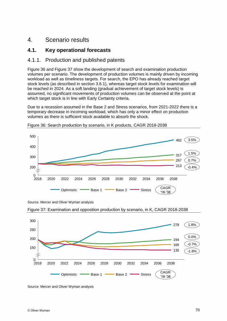
© Oliver Wyman 70

4. Scenario results

4.1. Key operational forecasts

4.1.1. Production and published patents

Figure 36 and Figure 37 show the development of search and examination production volumes per scenario. The development of production volumes is mainly driven by incoming workload as well as timeliness targets. For search, the EPO has already reached target stock levels (as described in section 3.6.1), whereas target stock levels for examination will be reached in 2024. As a soft landing (gradual achievement of target stock levels) is assumed, no significant movements of production volumes can be observed at the point at which target stock is in line with Early Certainty criteria.

Due to a recession assumed in the Base 2 and Stress scenarios, from 2021-2022 there is a temporary decrease in incoming workload, which has only a minor effect on production volumes as there is sufficient stock available to absorb the shock.

Figure 36: Search production by scenario, in K products, CAGR 2018-2038


Figure 37: Examination and opposition production by scenario, in K, CAGR 2018-2038


20362020 202620242018 2022 2028 2030 2032 2034 20380

200

300

400

500

213

462

317

267

Optimistic StressBase 2Base 1

3.5%

0.7%

1.5%

-0.4%

CAGR

’18-’38

202620202018 2022

300

2024 2028 2030 2032 2034 2036 20380

150

200

250

135

278

194

166

Optimistic Base 2Base 1 StressCAGR

’18-’38

1.8%

-0.7%

0.0%

-1.8%

© Oliver Wyman 71

Figure 38 shows the development of the number of published patents over time in each scenario. The number of published patents is strongly correlated to the number of examinations conducted and is driven by the same trends. It should be noted that the figures shown reflect patents published by the EPO and not the total number of patents validated in the member states.

Figure 38: Published patents by scenario, in K, CAGR 2018-2038


4.1.2. Workforce

To process incoming workload as well as stock with a given productivity, workforce is determined as described in section 3.6.3. Thus, the resulting examiner workforce is strongly dependent on the incoming workload influenced by the macroeconomic scenario.

In the Base 2 and Stress scenarios, workforce initially decreases to avoid potential temporary overcapacity in the short- to medium-term. After this initial decrease, examiner workforce grows or declines in line with incoming workload resulting in growth rates of -0.6% to 3.2% p.a. from 2018 to 2038 in the Stress and Optimistic scenario respectively. No additional leavers are assumed beyond not replacing retiring employees.

It is important to note that the workforce development applied in the model and shown in Figure 39 is not a recommendation on required workforce evolution for the EPO but a derived figure resulting from assumptions made on development of productivity and stock.

203620322018 20242020 2022 2026 2028 2030 2034 20380

100

150

200

183

128

110

89

Base 2Optimistic Base 1 StressCAGR

’18-’38

1.8%

-0.8%

0.0%

-1.8%

© Oliver Wyman 72

Figure 39: Examiner Workforce development, in paid man-years, by scenario, 2018–2038


In certain years, when examiner capacity exceeds incoming workload, a replacement ratio of zero is assumed, i.e. retiring examiners are not replaced (see Figure 40). Financially, this is sensible to avoid overcapacity and reduce costs. However, from a managerial perspective, this assumption should be reviewed in terms of actual operational requirements (e.g. certain skillsets/ sectoral know-how needed), feasibility and public perception (e.g. recruiting considerations).

Figure 40: Examiner replacement ratio by scenario, 2018–2038


4.1.3. Stock

In the short-term stock levels are primarily determined by incoming workload and available production capacity. In the long run workforce is set such that stock is in line with target stock in this study. As described in section 3.6.1 target stock is assumed as 5 output months of the production potentially possible with a given workforce for search and 25 months for examination.

In Figure 41 the development of stock of pending cases is shown for all scenarios. In the initial period covered by the study stock decreases due to increased productivity and subsequent reduction of examination stock. For Optimistic, Base 1 and Base 2 scenarios

202620242020 20362018 2022 2028 2030

8,000

2032

5,000

2034 20380

4,000

6,000

7,000

9,000

8,111

5,587

4,718

3,818

Optimistic Base 1 StressBase 2CAGR

’18-’38

3.2%

0.4%

1.3%

-0.6%

1.85

1.34

1.16

1.041.0

20322018 20282020 20362022 2024 2026 2030 2034 20380.0

2.0

3.0

4.0

5.0

Base 2Optimistic Base 1 Stress

© Oliver Wyman 73

stock increases again at a certain point. For these scenarios growth rates for the full period between 2018 and 2038 vary between -1.5% p.a. (Base 2 scenario) and +1.1% p.a. (Optimistic scenario). The stress scenario exhibits a growth rate of -2.6% p.a.

It is important to note that stock is constant in the long run in terms of output months and hence in line with the target stock (defined in output months). However, the actual number of cases in stock increases as output months are defined in terms of production capacity that can be delivered with a given examiner workforce and productivity. If incoming workload increases over time, workforce needs to increase as well and hence production capacity increases. Subsequently, once a steady state is reached the absolute number of cases in stock increases over time for all scenarios but the Stress scenario.

Figure 41: Cumulated search and examination stock (cases), by scenario 2018-2038, in K


4.2. Pension results

Figure 42 shows the projected IFRS DBO over 20 years for the Financial Study Base 2 scenario for funded plans (OPS, NPS, Health and LTC) and unfunded plans (Tax, Family Allowance and Death):

Figure 42: Projected IFRS DBO in Base 2 scenario over 20 years, in MN€


2018 20222020 2024 2026 2028 2030 2032 2034 2036

700

20380

400

500

600

800

900

808

565

483

387

Optimistic StressBase 1 Base 2

1.1%

-1.5%

-0.7%

-2.6%

CAGR

’18-’38

0

10,000

20,000

30,000

5,000

15,000

25,000

19,148

3,26136

14,481

448

1,683

8741,974

3,029

12

2018

592

2,767

2038

TaxDeath LTCFamily Allowance Health Pensions

20,841 MN€ 27,463 MN€

© Oliver Wyman 74

Despite large remeasurement effects of the DBO due to an increase in the IFRS discount rate assumed in the Base 2 scenario the DBO increases over the projection horizon to a value of 27,463 MN€. The increase is driven by the new hires and future accrual of active employees. As an example, the replacement ratio for examiners in the Base 2 scenario is 1.1. All benefits remain as-is.

4.3. Key financial forecasts

The EPO’s IFRS financial statements have been forecasted for a time horizon of 20 years. In this section the development of the EPO’s key balance sheet positions, revenue and cost components as well as operating cash flow is presented61. Detailed projections of the EPO’s balance sheet, its profit and loss statement and its cash flow statement can be found in Appendix A.

4.3.1. Statement of Financial Position

With -10,803 MN€ as of December 31st, 2018, the EPO currently has significantly negative equity. This situation is expected to improve over the time horizon of the study. In all scenarios equity improves until 2038 compared to 2018. However, only in the Optimistic scenario does the EPO manage to achieve positive equity, driven by positive market returns for RFPSS and EPOTIF and a lower benefit valuation. The IFRS discount rate in the Optimistic scenario is 5.0% in 2038 (Base 1 scenario: 4.7%; Base 2/ Stress scenario: 3.9%).

Figure 43: Equity – All scenarios forecast [IFRS], in MN€


For the Base 2 and Stress scenario a financial crisis is assumed. As a result, equity peaks in 2020 primarily driven by higher AA credit spread effects on defined benefit liabilities.

Total assets increase with operating surplus and with income and gains RFPSS and EPOTIF can generate over time.

Despite future accrual of active employees and new hires, liabilities remain relatively stable over time due to positive remeasurement effects.


20262018 2024

3,000

-3,0002020 2022 2028 2030

-12,000

2032 2034 2036 2038

-9,000

-6,000

0

6,0004,551

-6,190

-1,867

-7,429

Optimistic Base 1 StressBase 2

© Oliver Wyman 75

Figure 44: Key components of the Statement of Financial Position – Base 2 scenario [IFRS], in MN€


For the purpose of this Financial Study, it has been assumed that cash generated from operations which is not used for investing activities is recognized as other financial assets in the Statement of Financial Position with the exception of 10 MN€ that are recognized as cash and cash equivalents. The development of these two positions including interest earned on other financial assets is shown in Figure 45. As can be seen all scenarios strictly increase until the end of the projection horizon although year-to-year changes decrease due to operating cash flow decreasing over time.

Figure 45: Cash and cash equivalents and other financial assets, All scenarios forecast [IFRS], in MN€


20262020 2036203220282018 20342022 2024 2030 2038

-20,000

-10,000

0

10,000

20,000

30,000

11,532

22,336

-10,804

22,562

28,752

-6,190

EquityTotal assets Total liabilities

1.3%

3.4%

2.7%

CAGR

’18-’38

8,000

20282018 20262024 20342020 2022 20322030 2036 2038

10,000

0

2,000

4,000

6,000

8,926

5,936

5,957

4,303

Optimistic Base 1 Base 2 Stress

24.4 %

21.9%

21.9%

20.0%

CAGR

’18-’38

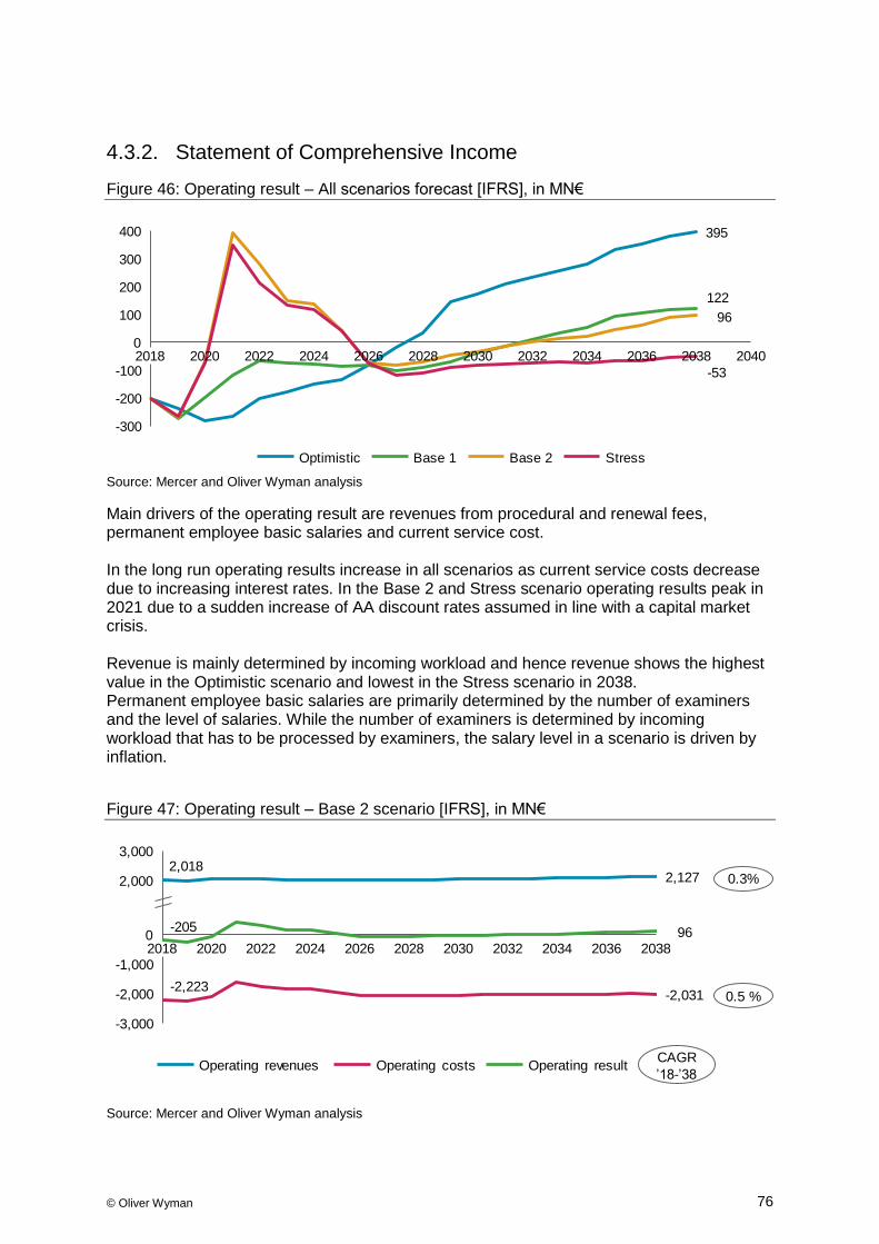
© Oliver Wyman 76

4.3.2. Statement of Comprehensive Income

Figure 46: Operating result – All scenarios forecast [IFRS], in MN€


Main drivers of the operating result are revenues from procedural and renewal fees, permanent employee basic salaries and current service cost. In the long run operating results increase in all scenarios as current service costs decrease due to increasing interest rates. In the Base 2 and Stress scenario operating results peak in 2021 due to a sudden increase of AA discount rates assumed in line with a capital market crisis. Revenue is mainly determined by incoming workload and hence revenue shows the highest value in the Optimistic scenario and lowest in the Stress scenario in 2038. Permanent employee basic salaries are primarily determined by the number of examiners and the level of salaries. While the number of examiners is determined by incoming workload that has to be processed by examiners, the salary level in a scenario is driven by inflation.

Figure 47: Operating result – Base 2 scenario [IFRS], in MN€


20402024 202620202018 2022 2028 2030

400

2032 2034 2036

-300

2038

-200

-100

0

100

200

300

96

395

122

-53


2028

-3,000

20262024

-2,000

20322018 20302020 2022 2034 2036 2038-1,000

0

2,000

3,0002,018

2,127

-2,031

96

-2,223

-205

0.3%

0.5 %

Operating revenues Operating costs Operating resultCAGR

’18-’38

© Oliver Wyman 77

4.3.3. Development of revenue from procedural and renewal fees

Revenue from procedural fees related to the Patent Grant Process

From 2018 to 2038, revenue from procedural fees (excluding Internal Renewal Fees) increases in all scenarios except the Stress scenario (see Figure 48). Key drivers underlying revenue from procedural fees are incoming workload as a key determinant of SEO production once stock is at target level and the ratio of search vs. examination production. The latter is relevant as examinations are, on average, associated with higher fees compared to searches while taking less examiner time.

Figure 48: Revenue from Procedural Fees - All scenarios forecast, in MN€


In the Optimistic scenario, revenue growth from procedural fees is based on substantial increases in incoming demand and SEO production which is tilted towards searches during the considered time period. Applications increase at 3.7% p.a. while incoming product orders (search) increase at 3.6% p.a. (see Figure 28 and Figure 29). This drives production of searches which grows at 3.5% p.a. and production of examinations and oppositions which grow at 1.8% p.a. (see Figure 36 and Figure 37)

In the Base 1 scenario, revenue grows slower than in the Optimistic scenario which is primarily driven by slower increases in incoming applications (1.7% p.a.) and new product orders (search) (1.6% p.a.) (see Figure 28 and Figure 29). This leads to lower SEO production figures than in the Optimistic scenario with a positive development of 1.5% p.a. for searches and 0.0% for examinations and opposition (see Figure 36 and Figure 37).

In the Base 2 scenario, revenue stagnates despite moderate growth of incoming applications (0.9% p.a. for applications and 0.8% p.a. for incoming product orders (search) – see Figure 28 and Figure 29). Even though search production grew at 0.7% p.a., examination and opposition production declined at 0.7% p.a. (see Figure 36 and Figure 37). This leads to constant figures of total SEO production over the 20-year period.

The negative revenue developments in the Stress scenario can be explained by decreasing incoming demand on the application and product orders (search) which lead to declining SEO production and thus, smaller revenue associated to procedural fees.

907730

20282018 202620242020 2022 2030 2032 2034 2036 20380

500

1,000

1,500

2,000

1,541

1,067


2.9%

1.0%

0.2%

-0.9%

CAGR

’18-’38

© Oliver Wyman 78

Revenue from renewal fees for patent applications (Internal renewal fees)

Revenues from internal renewal fees are determined by the number and duration of cases in stock. Over the time horizon of the Financial Study, revenue from internal renewal fees increases only in the Optimistic scenario and decreases in the Base 1, Base 2 and Stress scenarios (see Figure 49). This results in growth rates from +0.5% p.a. in the Optimistic scenario to -3.1% p.a. in the Stress scenario.

From 2018 to approximately the year 2028 revenues from internal renewal fees decrease in all scenarios due to a reduction in cases pending and a shift in the age structure of those cases. This is caused by an increase in productivity compared to previous years due to the effort to fulfill Early Certainty criteria. Once a steady state is reached between production capacity stock and incoming workload, revenues from internal renewal fees increase corresponding to the increase of incoming workload and thus the target stock.

Figure 49: Revenue from Internal Renewal Fees - All scenarios forecast, in MN€


Revenue from national renewal fees for granted patents

National renewal fees are less sensitive to changes in the macroeconomic environment (which drives incoming workload) in the near term as they are paid over the complete lifetime of a patent once it has been granted by the EPO. Hence, until approximately the year 2029 revenues from NRFs show very little deviation between scenarios.

During this time, they increase substantially in all scenarios with a growth rate between 3.2% p.a. in the Stress scenario and 3.9% p.a. in the Optimistic scenario. This is caused by a strong increase in the number of patents that are granted by the EPO and enter the population of NRF-paying patents, which has already been seen in the past years and is predicted to continue in the future depending on the incoming workload.

After this period of synchronized growth, effects of different levels of incoming workload between the scenarios become visible. Revenue from NRFs continues to grow for the Optimistic scenario resulting in a growth rate of +3.8% p.a. for the full period from 2018 to 2038 as well as for the Base 1 scenario resulting in a growth rate of +2.4% p.a. for the full period from 2018 to 2038. For the Base 2 scenario, growth ceases after 2029 resulting in a growth rate of 1.9% p.a. for the full period from 2018 to 2038 whereas growth decreases for

573

401343

275

2026

400

2018 20300

20282020 2022 20322024 2034 2036

600

2038

100

200

300

500

Base 1Optimistic StressBase 2

0.5%

-1.3%

- 2.1%

-3.1%

CAGR

’18-’38

© Oliver Wyman 79

the Stress scenario resulting in a growth rate of +1.3% p.a.) for the full period from 2018 to 2038.

Figure 50: Revenue from National Renewal Fees - All scenarios forecast, in MN€


4.3.4. Statement of Cash Flows

Operating cash flow is generated from the EPO’s activities related to the PGP. In this context RPFSS is considered as an entity separate from the Office. It is assumed that pension and social security contributions from staff and the Office are transferred to RFPSS and payments related to pensions and other benefits are made by RFPSS as of 2019.

For the purpose of this study, the direct approach for calculating the EPO’s operating cash flow has been chosen over the indirect one to better illustrate the effects of major financial drivers within the EPO’s operations on its liquidity position.

Operating cash flow62 in all scenarios except the Optimistic scenario exhibits a long-term downward trend. This is driven by lower growth of cash proceeds in relation to expenses.63 Particularly, if fees do not grow in line with employee benefit payments this inevitably leads to a long-term structural problem in the EPO’s cost-coverage. A negative peak in 2019 is caused by lower expected production levels which is then overcompensated in 2020 by increases in revenue from national renewal fees and higher revenue from procedural fees due to processing of newer files.

Family allowance, tax compensation for OPS pension payments64 and Death benefits65 are unfunded and are paid by the Office out of the operating cash flow. Given the decrease in cash flow, the EPO is at risk of not being able to pay unfunded benefits out of the operating cash flow and hence needs to put aside a reserve while operating cash flow is positive. A sufficient reserve could be built in the EPOTIF over time and future cash flows for unfunded employee benefits could be served by activating the fund assets. Additional contributions to

62 Deviations to cash flow reported in financial statements 2018 are driven by differing classification of cash items

as non-operational. Operating cash flow is approximated using the direct approach.

63 Fees assumed to remain at current levels except for a one-off fee increase in procedural and internal renewal fees of 4% in 2020

64 As of December 2018, ca 87 MN€ of RFPSS assets are reserved for OPS tax compensation (1.1% of total assets) are allowed for in the study but are not enough to cover benefit payments.

65 Death benefits are unfunded, but a separate contribution rate covers annual payments.

881

787

703

203020242018 2026

600

2020 2022 2028 2032 2034 2036 20380

200

400

800

1,000

1,200 1,156

Optimistic Base 1 Base 2 StressCAGR

’18-’38

3.8%

2.4%

1.9%

1.3%

© Oliver Wyman 80

accumulate a reserve for funded pensions can also only be undertaken during the next 10 years while operating cash flow is significantly positive. However, as can be seen in section 4.4 closing the coverage gap is only possible in the Optimistic scenario. This means that in the other scenarios, even if cash flow remains positive, the benefit funding gap is forecasted to surpass available cash surplus in 2038.

Figure 51: Operating cash flow (Direct approach – Office view) – All scenarios forecast [IFRS], in MN€, 2018–2038


Figure 52 and Figure 53 below demonstrate the structural challenges related to its cost base that the EPO is facing. Cash proceeds from fee income grow slower over time than basic salary costs including allowances. This is reflected in the reduction of net operating cash flow generated by examiner over time by about one third, namely from 109.2 K€ (average 2016-2018) to 76.4 K€ (average 2018 to 2038).

Figure 52: Fee cash proceeds and salaries per examiner in K€, Base 2 scenario, IFRS view


2024 20282018 2020 203220262022 2030 2034 2036 20380

100

200

300

400

500

171

392

136

2


Average 2016-18 Average 2018-28 Average 2018-38

440.8

284.7

465.8

315.3

458.4

321.5

-35%-32% -30%

Cash proceeds from fees (procedural, IRF and NRF)

Basic salaries permanent employees, allowances and office contributions to social security

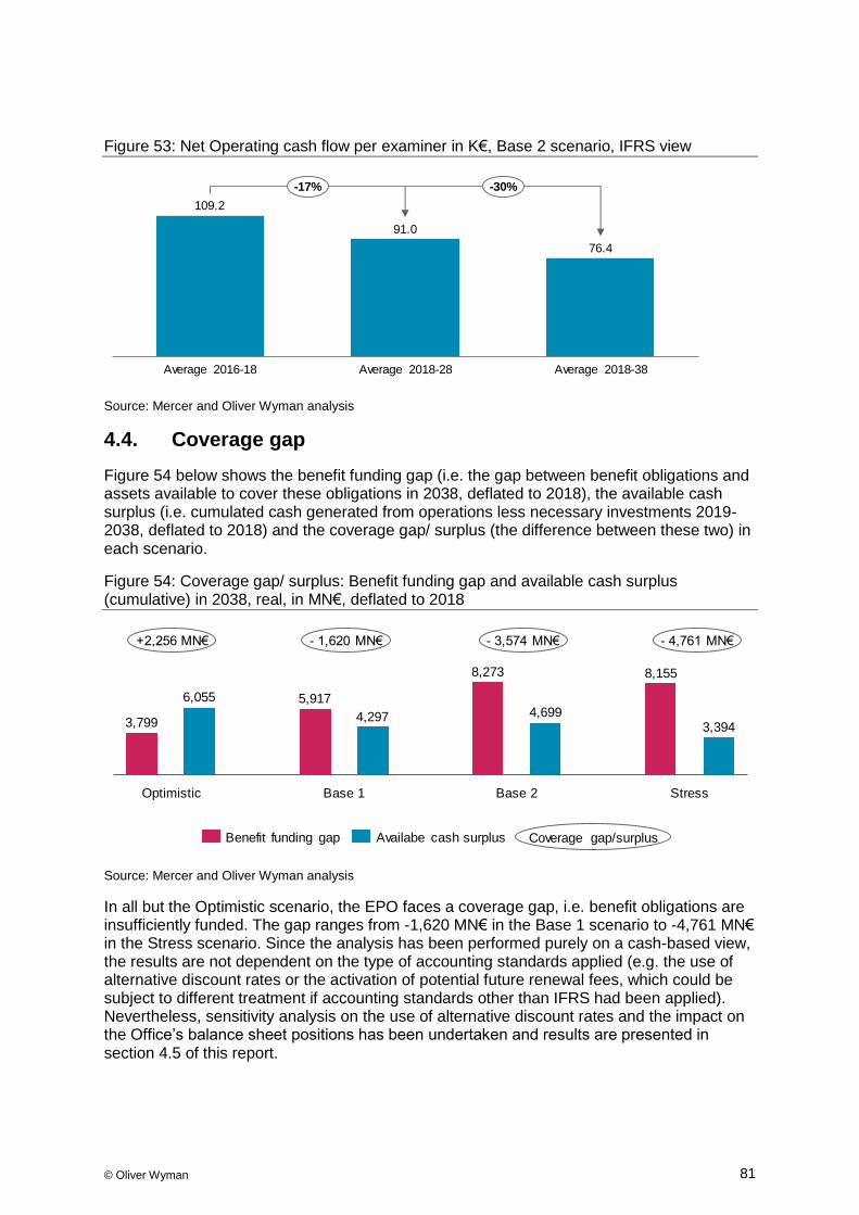
© Oliver Wyman 81

Figure 53: Net Operating cash flow per examiner in K€, Base 2 scenario, IFRS view


4.4. Coverage gap

Figure 54 below shows the benefit funding gap (i.e. the gap between benefit obligations and assets available to cover these obligations in 2038, deflated to 2018), the available cash surplus (i.e. cumulated cash generated from operations less necessary investments 2019-2038, deflated to 2018) and the coverage gap/ surplus (the difference between these two) in each scenario.

Figure 54: Coverage gap/ surplus: Benefit funding gap and available cash surplus (cumulative) in 2038, real, in MN€, deflated to 2018


In all but the Optimistic scenario, the EPO faces a coverage gap, i.e. benefit obligations are insufficiently funded. The gap ranges from -1,620 MN€ in the Base 1 scenario to -4,761 MN€ in the Stress scenario. Since the analysis has been performed purely on a cash-based view, the results are not dependent on the type of accounting standards applied (e.g. the use of alternative discount rates or the activation of potential future renewal fees, which could be subject to different treatment if accounting standards other than IFRS had been applied). Nevertheless, sensitivity analysis on the use of alternative discount rates and the impact on the Office’s balance sheet positions has been undertaken and results are presented in section 4.5 of this report.

Average 2018-38

91.0

Average 2016-18 Average 2018-28

109.2

76.4

-17% -30%

4,6993,799

8,273

6,055 5,917

8,155

4,2973,394

Benefit funding gap Availabe cash surplus Coverage gap/surplus

+2,256 MN€ - 1,620 MN€ - 3,574 MN€ - 4,761 MN€


© Oliver Wyman 82

The discount rate does not reflect the RFPSS’ long-term return objective. For that reason, financial sustainability is evaluated with a valuation by applying RFPSS’ long-term return expectation which can be achieved with a sufficiently large confidence, i.e. prudent discount rate. That is, the real discount rate of 2.1% is achieved in 2/3 of stochastic capital market scenarios. Applying the prudent discount rate, the real benefit funding gap in 2038 for the Base 2 scenario is summarized in the following Table 9:

Table 9: Benefit funding gap, cash surplus & coverage gap in Base 2 scenario, in MN€

Balance sheet item 2038 IFRS Statement

2038 Nominal Funding Valuation 2038 Real Funding Valuation4

1. Defined-benefit obligation

27,463 26,344 influenced by prudent

discount rate: 2.1% real p.a.

20,782

2. RFPSS1 11,221 influenced by scenario YoY returns

(2019-2038) and net payments; market value, independent of

accounting standards

8,852

3. EPOTIF2 4,635 influenced by scenario YoY returns

(2019-2038); market value, independent of accounting

standards

3,657

4. Cash surplus3 5,957 sum of operating cash flow (2019-

2038)

4,699

5. Benefit funding gap (=(1)-(2)-(3))

8,273

6. Coverage gap

(=(5)-(4))

3,574


Notations:

1. RFPSS is assumed to be activated, i.e. benefit payments of funded plans are financed by the assets of RFPSS.

2. There are no contributions to and no payments from EPOTIF assumed.

3. Cash surplus is the accumulated operating cash flow over the projection horizon of 20 years.

4. The applied discount rate is the YoY inflation which refers to HICP. Over the 20-year projection horizon, the average inflation rate in the Base 2 scenario is 1.2%.

The benefit funding gap and the coverage gap from a funding valuation perspective are indicators that reflect the EPO’s sustainability and the assets required to cover all benefit payments in the future. The funding valuation approach is used to detach the analysis from IFRS discount rate. In the Base 2 scenario the real funding DBO is 20,782 MN€. The real funding DBO of pensions, LTC and Health needs to be covered by RFPSS. EPOTIF is also

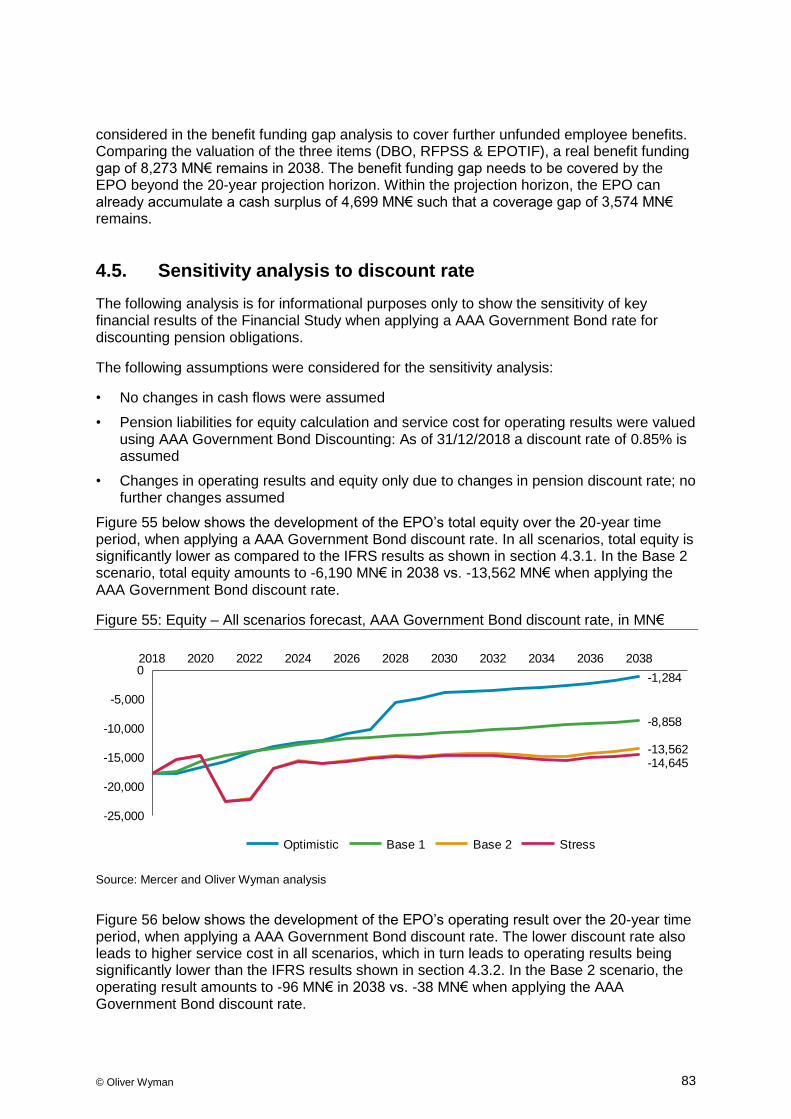
© Oliver Wyman 83

considered in the benefit funding gap analysis to cover further unfunded employee benefits. Comparing the valuation of the three items (DBO, RFPSS & EPOTIF), a real benefit funding gap of 8,273 MN€ remains in 2038. The benefit funding gap needs to be covered by the EPO beyond the 20-year projection horizon. Within the projection horizon, the EPO can already accumulate a cash surplus of 4,699 MN€ such that a coverage gap of 3,574 MN€ remains.

4.5. Sensitivity analysis to discount rate

The following analysis is for informational purposes only to show the sensitivity of key financial results of the Financial Study when applying a AAA Government Bond rate for discounting pension obligations.

The following assumptions were considered for the sensitivity analysis:

• No changes in cash flows were assumed

• Pension liabilities for equity calculation and service cost for operating results were valued using AAA Government Bond Discounting: As of 31/12/2018 a discount rate of 0.85% is assumed

• Changes in operating results and equity only due to changes in pension discount rate; no further changes assumed

Figure 55 below shows the development of the EPO’s total equity over the 20-year time period, when applying a AAA Government Bond discount rate. In all scenarios, total equity is significantly lower as compared to the IFRS results as shown in section 4.3.1. In the Base 2 scenario, total equity amounts to -6,190 MN€ in 2038 vs. -13,562 MN€ when applying the AAA Government Bond discount rate.

Figure 55: Equity – All scenarios forecast, AAA Government Bond discount rate, in MN€


Figure 56 below shows the development of the EPO’s operating result over the 20-year time period, when applying a AAA Government Bond discount rate. The lower discount rate also leads to higher service cost in all scenarios, which in turn leads to operating results being significantly lower than the IFRS results shown in section 4.3.2. In the Base 2 scenario, the operating result amounts to -96 MN€ in 2038 vs. -38 MN€ when applying the AAA Government Bond discount rate.

20302024 20282020 20222018 2026

-15,000

2032 2034 2036 2038

-25,000

0

-20,000

-10,000

-5,000

-14,645

-1,284

-8,858

-13,562


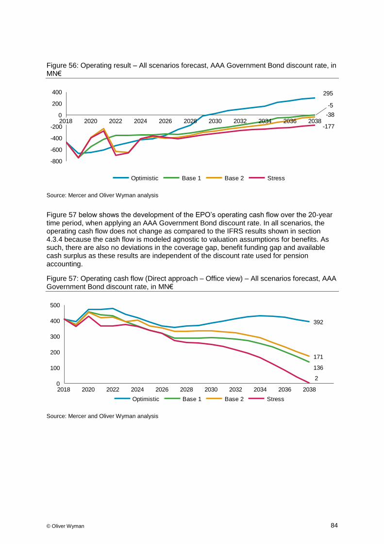
© Oliver Wyman 84

Figure 56: Operating result – All scenarios forecast, AAA Government Bond discount rate, in MN€


Figure 57 below shows the development of the EPO’s operating cash flow over the 20-year time period, when applying an AAA Government Bond discount rate. In all scenarios, the operating cash flow does not change as compared to the IFRS results shown in section 4.3.4 because the cash flow is modeled agnostic to valuation assumptions for benefits. As such, there are also no deviations in the coverage gap, benefit funding gap and available cash surplus as these results are independent of the discount rate used for pension accounting.

Figure 57: Operating cash flow (Direct approach – Office view) – All scenarios forecast, AAA Government Bond discount rate, in MN€


20282022 20262018 2020

-800

20362024 2030 2032 2034 2038

-600

-400

-200

0

200

400

-177

-38

295

-5


2024 203002018 20282020 20262022 2032 2034 2036 2038

100

200

400

300

500

392

136

171

2


© Oliver Wyman 85

4.6. Summary of scenario results

The study results convey the following key messages:

Pension payments will triple by 2038 and benefit liabilities will not be completely covered by cash reserves in 2038: Due to the significant number of retiring employees in the coming years and a structurally maturing workforce, the EPO's benefit payments are expected to triple over the next 20 years. Depending on the scenario, additional contributions of between 1.6 BN€ and 4.8 BN€ (real) will be required to have sufficiently high funding levels for benefits from 2038 onwards. This is in addition to reserves that have already been put aside in the EPOTIF.

There is a significant benefit funding gap to be closed: Depending on the scenario, the benefit funding gap between required and available assets to cover for all future and accrued benefit payments from 2038 onwards is between 3.8 BN€ and 8.3 BN€ in real terms. The EPO currently does not have sufficient asset reserves to cover these requirements.

With key parameters not changed, the operation will experience a gradual reduction in cash: The EPO faces a structural operational gap, with costs increasing faster than revenues, leading in the future to significantly decreasing cash flows. On the current path, costs will continue to increase faster than revenues and the EPO will face significantly decreasing cash flows in the “Base 1: Economic Recovery”, “Base 2: Economic Cycle” and Stress scenario.

A time-limited window of opportunity to act is open now: The window of opportunity to build up necessary reserves and buffers is open now while the EPO’s cash flow is still sufficiently high. At the moment, the probability that asset returns can fully cover future and accrued benefits payments is 40% and this could be increased to a 66% probability by applying a more prudent discount rate to funding valuation. Although there are still scenarios (the remaining 34%) with severe market downturns which lead to cases where returns are not sufficient to cover all future benefit payments, the likelihood of this is significantly smaller. In these cases, the benefit payments are dependent on the Office to continue generating sufficient cash. Please note that this has no direct effect on contribution rates, but the EPO can build up a risk buffer in case of market stress or other unforeseen events to ensure the long-term sustainability of employee benefits. Each year during which these actions are deferred will negatively impact the probability that benefit payments will be fully funded in the long-term.

The EPO has greater control to manage its long-term cost structure than its revenue: Taking a prudent approach to managing long-term financial sustainability, the EPO needs to evaluate the structural gaps between revenue and cost. There is little room for manoeuver through driving increased revenue which is influenced by stakeholders such as the Member States. However, the EPO has greater control of cost levers, which presents an opportunity to better meet its future obligations through careful cost management.

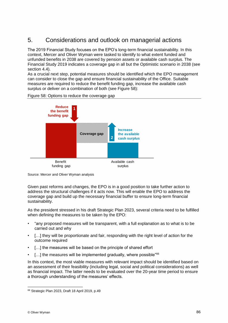
© Oliver Wyman 86

5. Considerations and outlook on managerial actions

The 2019 Financial Study focuses on the EPO’s long-term financial sustainability. In this context, Mercer and Oliver Wyman were tasked to identify to what extent funded and unfunded benefits in 2038 are covered by pension assets or available cash surplus. The Financial Study 2019 indicates a coverage gap in all but the Optimistic scenario in 2038 (see section 4.4). As a crucial next step, potential measures should be identified which the EPO management can consider to close the gap and ensure financial sustainability of the Office. Suitable measures are required to reduce the benefit funding gap, increase the available cash surplus or deliver on a combination of both (see Figure 58):

Figure 58: Options to reduce the coverage gap


Given past reforms and changes, the EPO is in a good position to take further action to address the structural challenges if it acts now. This will enable the EPO to address the coverage gap and build up the necessary financial buffer to ensure long-term financial sustainability.

As the president stressed in his draft Strategic Plan 2023, several criteria need to be fulfilled when defining the measures to be taken by the EPO:

• “any proposed measures will be transparent, with a full explanation as to what is to be carried out and why

• […] they will be proportionate and fair, responding with the right level of action for the outcome required

• […] the measures will be based on the principle of shared effort

• […] the measures will be implemented gradually, where possible”66

In this context, the most viable measures with relevant impact should be identified based on an assessment of their feasibility (including legal, social and political considerations) as well as financial impact. The latter needs to be evaluated over the 20-year time period to ensure a thorough understanding of the measures’ effects.

66 Strategic Plan 2023, Draft 18 April 2019, p.49

Benefit

funding gap

Available cash

surplus

Coverage gap

Reduce the benefit

funding gap

Increase the available cash surplus

1

2

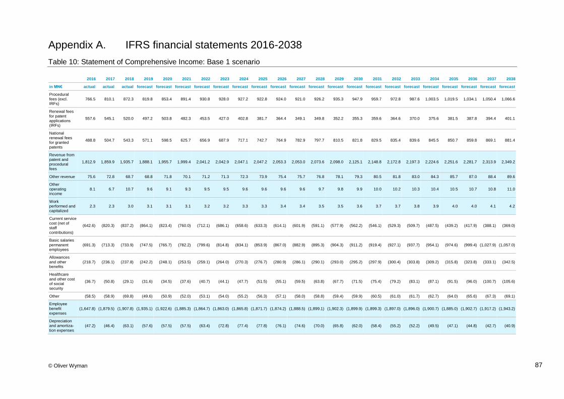
© Oliver Wyman 87

Appendix A. IFRS financial statements 2016-2038

Table 10: Statement of Comprehensive Income: Base 1 scenario

2016 2017 2018 2019 2020 2021 2022 2023 2024 2025 2026 2027 2028 2029 2030 2031 2032 2033 2034 2035 2036 2037 2038

in MN€ actual actual actual forecast forecast forecast forecast forecast forecast forecast forecast forecast forecast forecast forecast forecast forecast forecast forecast forecast forecast forecast forecast

Procedural fees (excl. IRFs)

766.5 810.1 872.3 819.8 853.4 891.4 930.8 928.0 927.2 922.8 924.0 921.0 926.2 935.3 947.9 959.7 972.8 987.6 1,003.5 1,019.5 1,034.1 1,050.4 1,066.6

Renewal fees for patent applications (IRFs)

557.6 545.1 520.0 497.2 503.8 482.3 453.5 427.0 402.8 381.7 364.4 349.1 349.8 352.2 355.3 359.6 364.6 370.0 375.6 381.5 387.8 394.4 401.1

National

renewal fees for granted patents

488.8 504.7 543.3 571.1 598.5 625.7 656.9 687.9 717.1 742.7 764.9 782.9 797.7 810.5 821.8 829.5 835.4 839.6 845.5 850.7 859.8 869.1 881.4

Revenue from patent and procedural fees

1,812.9 1,859.9 1,935.7 1,888.1 1,955.7 1,999.4 2,041.2 2,042.9 2,047.1 2,047.2 2,053.3 2,053.0 2,073.6 2,098.0 2,125.1 2,148.8 2,172.8 2,197.3 2,224.6 2,251.6 2,281.7 2,313.9 2,349.2

Other revenue 75.6 72.8 68.7 68.8 71.8 70.1 71.2 71.3 72.3 73.9 75.4 75.7 76.8 78.1 79.3 80.5 81.8 83.0 84.3 85.7 87.0 88.4 89.6

Other operating income

8.1 6.7 10.7 9.6 9.1 9.3 9.5 9.5 9.6 9.6 9.6 9.6 9.7 9.8 9.9 10.0 10.2 10.3 10.4 10.5 10.7 10.8 11.0

Work performed and capitalized

2.3 2.3 3.0 3.1 3.1 3.1 3.2 3.2 3.3 3.3 3.4 3.4 3.5 3.5 3.6 3.7 3.7 3.8 3.9 4.0 4.0 4.1 4.2

Current service cost (net of staff contributions)

(642.6) (820.3) (837.2) (864.1) (823.4) (760.0) (712.1) (686.1) (658.6) (633.3) (614.1) (601.9) (591.1) (577.9) (562.2) (546.1) (529.3) (509.7) (487.5) (439.2) (417.9) (388.1) (369.0)

Basic salaries

permanent employees

(691.3) (713.3) (733.9) (747.5) (765.7) (782.2) (799.6) (814.8) (834.1) (853.9) (867.0) (882.9) (895.3) (904.3) (911.2) (919.4) (927.1) (937.7) (954.1) (974.6) (999.4) (1,027.9) (1,057.0)

Allowances

and other benefits

(218.7) (236.1) (237.8) (242.2) (248.1) (253.5) (259.1) (264.0) (270.3) (276.7) (280.9) (286.1) (290.1) (293.0) (295.2) (297.9) (300.4) (303.8) (309.2) (315.8) (323.8) (333.1) (342.5)

Healthcare

and other cost of social security

(36.7) (50.8) (29.1) (31.6) (34.5) (37.6) (40.7) (44.1) (47.7) (51.5) (55.1) (59.5) (63.8) (67.7) (71.5) (75.4) (79.2) (83.1) (87.1) (91.5) (96.0) (100.7) (105.6)

Other (58.5) (58.9) (69.8) (49.6) (50.9) (52.0) (53.1) (54.0) (55.2) (56.3) (57.1) (58.0) (58.8) (59.4) (59.9) (60.5) (61.0) (61.7) (62.7) (64.0) (65.6) (67.3) (69.1)


(1,647.8) (1,879.5) (1,907.8) (1,935.1) (1,922.6) (1,885.3) (1,864.7) (1,863.0) (1,865.8) (1,871.7) (1,874.2) (1,888.5) (1,899.1) (1,902.3) (1,899.9) (1,899.3) (1,897.0) (1,896.0) (1,900.7) (1,885.0) (1,902.7) (1,917.2) (1,943.2)

Depreciation and amortiza-tion expenses

(47.2) (46.4) (63.1) (57.6) (57.5) (57.5) (63.4) (72.8) (77.4) (77.8) (76.1) (74.6) (70.0) (65.8) (62.0) (58.4) (55.2) (52.2) (49.5) (47.1) (44.8) (42.7) (40.9)

© Oliver Wyman 88

2016 2017 2018 2019 2020 2021 2022 2023 2024 2025 2026 2027 2028 2029 2030 2031 2032 2033 2034 2035 2036 2037 2038


Other operating expenses

(213.2) (222.8) (252.1) (253.9) (256.5) (259.4) (262.5) (265.9) (269.5) (273.5) (277.8) (282.4) (287.3) (292.2) (297.4) (302.9) (308.7) (314.7) (320.7) (327.1) (333.8) (340.9) (348.2)

Operating result

(9.4) (207.0) (204.8) (277.0) (196.9) (120.2) (65.5) (74.7) (80.6) (89.1) (86.5) (103.8) (92.7) (70.9) (41.4) (17.7) 7.6 31.5 52.3 92.6 102.2 116.4 121.7

Income and gains on RFPSS assets (net)

537.6 672.1 (523.3) 338.6 327.4 341.3 373.4 395.5 417.1 445.7 470.2 500.6 524.3 547.8 572.7 599.0 619.6 647.6 664.5 693.7 710.8 730.6 752.5

Income &

gains on EPOTIF assets (net)

17.7 14.1 8.7 99.6 97.9 101.3 108.4 113.6 118.9 125.7 131.9 139.6 146.2 153.1 160.7 169.0 176.6 186.3 194.3 205.6 215.0 225.7 237.7

Interest income from bank accounts and deposits

0.5 0.2 0.1 - (2.1) (2.2) (0.7) 1.1 3.8 7.9 12.3 17.5 22.9 29.2 36.4 43.9 51.5 60.7 69.5 79.9 88.9 98.7 108.6

Other 7.6 9.4 12.4 - - - - - - - - - - - - - - - - - - - -

Finance revenue

563.3 695.8 (502.2) 438.3 423.3 440.4 481.0 510.2 539.8 579.3 614.4 657.7 693.4 730.1 769.8 811.9 847.7 894.6 928.2 979.2 1,014.7 1,055.0 1,098.7

Interest costs on defined benefit obligations

(410.7) (366.0) (358.9) (418.1) (439.9) (473.3) (521.3) (563.4) (606.8) (652.7) (697.3) (744.2) (788.7) (834.4) (881.4) (927.8) (974.9) (1,024.7) (1,070.4) (1,117.7) (1,160.4) (1,205.1) (1,247.5)

Other (3.8) (6.5) (91.3) - - - - - - - - - - - - - - - - - - - -

Finance costs (414.5) (372.4) (450.1) (418.1) (439.9) (473.3) (521.3) (563.4) (606.8) (652.7) (697.3) (744.2) (788.7) (834.4) (881.4) (927.8) (974.9) (1,024.7) (1,070.4) (1,117.7) (1,160.4) (1,205.1) (1,247.5)

Financial result

148.9 323.4 (952.3) 20.2 (16.7) (32.9) (40.3) (53.2) (67.0) (73.4) (82.9) (86.5) (95.2) (104.3) (111.6) (115.9) (127.2) (130.1) (142.2) (138.5) (145.7) (150.1) (148.8)

Profit/ (loss)

for the year 139.4 116.4 (1,157.2) (256.8) (213.6) (153.1) (105.9) (127.9) (147.6) (162.4) (169.4) (190.4) (188.0) (175.2) (153.0) (133.6) (119.6) (98.6) (89.8) (45.8) (43.5) (33.6) (27.1)

Other compre-hensive income

(2,980.7) (347.0) 1,285.7 (192.8) 1,481.6 1,213.0 849.1 818.2 824.5 677.8 622.4 500.0 504.9 519.1 529.4 447.5 465.4 420.0 496.0 362.9 362.6 373.9 295.9

Total com-prehensive income for the year

(2,841.3) (230.6) 128.5 (449.6) 1,268.1 1,059.9 743.2 690.3 676.9 515.4 453.0 309.7 317.0 344.0 376.4 313.9 345.8 321.4 406.1 317.0 319.1 340.3 268.8

© Oliver Wyman 89

Table 11: Statement of Financial Position: Base 1 scenario

2016 2017 2018 2019 2020 2021 2022 2023 2024 2025 2026 2027 2028 2029 2030 2031 2032 2033 2034 2035 2036 2037 2038


Property, plant and equipment

576.8 647.2 661.8 661.0 660.3 731.6 845.0 901.1 904.6 883.9 864.8 808.3 756.4 708.8 665.1 625.0 588.2 554.5 523.5 495.1 468.9 445.0 423.0

Intangible assets 48.8 50.4 38.4 37.5 38.8 39.6 40.4 40.5 40.6 40.6 40.7 40.7 41.1 41.6 42.2 42.7 43.1 43.6 44.2 44.7 45.3 46.0 46.7

RFPSS net assets

7,292.2 8,193.8 7,901.8 8,286.7 8,651.4 9,018.9 9,406.4 9,800.4 10,200.5 10,611.3 11,024.5 11,443.3 11,857.3 12,262.8 12,658.2 13,042.1 13,405.1 13,752.8 14,074.6 14,383.2 14,666.6 14,927.8 15,169.9

EPOTIF (including current assets)

1,571.2 1,880.9 2,460.2 2,559.8 2,657.7 2,759.0 2,867.4 2,981.0 3,099.9 3,225.6 3,357.5 3,497.1 3,643.3 3,796.4 3,957.1 4,126.1 4,302.6 4,489.0 4,683.2 4,888.8 5,103.8 5,329.5 5,567.1

Home loans to staff

87.7 87.2 88.2 86.1 89.1 91.0 92.9 92.9 93.2 93.2 93.6 93.6 94.5 95.7 96.9 98.0 99.1 100.2 101.5 102.7 104.1 105.6 107.2

Other financial assets

77.0 58.0 - 424.9 817.8 1,121.7 1,372.5 1,635.9 1,924.0 2,209.7 2,482.6 2,769.4 3,059.2 3,355.1 3,661.1 3,970.6 4,283.5 4,595.5 4,899.4 5,188.6 5,458.3 5,703.4 5,925.8

Other assets 117.3 140.1 86.8 - - - - - - - - - - - - - - - - - - - -

Non-current assets

9,771.0 11,057.7 11,237.1 12,055.9 12,915.2 13,761.8 14,624.6 15,451.8 16,262.7 17,064.2 17,863.7 18,652.4 19,451.9 20,260.4 21,080.7 21,904.5 22,721.8 23,535.6 24,326.4 25,103.2 25,847.0 26,557.2 27,239.7

Trade and other receivables

162.2 172.1 154.9 151.2 156.6 159.8 163.1 163.3 163.7 163.8 164.4 164.4 166.1 168.1 170.2 172.2 174.1 176.1 178.3 180.5 182.9 185.5 188.3

Bonds 234.9 379.2 - - - - - - - - - - - - - - - - - - - - -

Home loans to staff

7.4 7.6 7.9 7.7 8.0 8.2 8.3 8.4 8.4 8.4 8.4 8.4 8.5 8.6 8.7 8.8 8.9 9.0 9.1 9.2 9.4 9.5 9.6


318.0 87.0 58.0 - - - - - - - - - - - - - - - - - - - -

Prepaid expenses

15.1 16.6 19.3 18.9 19.5 19.9 20.4 20.4 20.4 20.4 20.5 20.5 20.7 21.0 21.2 21.5 21.7 22.0 22.3 22.5 22.8 23.2 23.5

Cash and cash equivalents

19.6 2.3 54.9 10.0 10.0 10.0 10.0 10.0 10.0 10.0 10.0 10.0 10.0 10.0 10.0 10.0 10.0 10.0 10.0 10.0 10.0 10.0 10.0

Current assets 757.2 664.9 295.0 187.8 194.1 197.9 201.8 202.0 202.5 202.6 203.3 203.3 205.3 207.6 210.2 212.4 214.7 217.1 219.7 222.3 225.1 228.2 231.5

Total assets 10,528.2 11,722.6 11,532.2 12,243.7 13,109.3 13,959.7 14,826.4 15,653.8 16,465.2 17,266.9 18,067.0 18,855.7 19,657.2 20,468.0 21,290.8 22,116.9 22,936.5 23,752.7 24,546.1 25,325.5 26,072.2 26,785.4 27,471.1

Retained earnings

(1,734.3) (1,617.9) (2,840.5) (3,097.3) (3,310.9) (3,464.0) (3,569.9) (3,697.8) (3,845.4) (4,007.8) (4,177.2) (4,367.6) (4,555.5) (4,730.7) (4,883.7) (5,017.3) (5,136.9) (5,235.5) (5,325.3) (5,371.2) (5,414.7) (5,448.3) (5,475.4)

Other compo-nents of equity

(8,902.0) (9,249.0) (7,963.3) (8,156.1) (6,674.4) (5,461.4) (4,612.3) (3,794.1) (2,969.6) (2,291.8) (1,669.4) (1,169.4) (664.4) (145.3) 384.1 831.6 1,297.0 1,717.0 2,213.0 2,575.9 2,938.4 3,312.4 3,608.3

Total equity (10,636.3) (10,866.8) (10,803.8) (11,253.3) (9,985.3) (8,925.4) (8,182.2) (7,491.8) (6,815.0) (6,299.6) (5,846.6) (5,536.9) (5,220.0) (4,876.0) (4,499.6) (4,185.7) (3,839.9) (3,518.5) (3,112.4) (2,795.3) (2,476.3) (2,136.0) (1,867.1)

Defined benefit liability

19,716.5 21,087.6 20,840.8 22,126.6 21,704.4 21,504.4 21,650.4 21,822.0 21,980.3 22,279.9 22,631.2 23,106.6 23,574.0 24,019.0 24,441.0 24,926.7 25,371.5 25,835.1 26,187.6 26,612.9 26,999.0 27,327.4 27,697.1

Salary Savings Plan obligation

58.2 79.6 86.4 - - - - - - - - - - - - - - - - - - - -

Other employee-related liabilities

21.7 38.3 23.6 40.2 41.2 42.1 43.0 43.8 44.8 45.9 46.6 47.5 48.1 48.6 49.0 49.4 49.8 50.4 51.3 52.4 53.7 55.3 56.8

Finance lease liabilities

2.4 2.4 1.9 1.8 1.9 1.9 2.0 2.0 2.0 2.0 2.0 2.0 2.0 2.0 2.0 2.1 2.1 2.1 2.1 2.2 2.2 2.2 2.3

© Oliver Wyman 90

2016 2017 2018 2019 2020 2021 2022 2023 2024 2025 2026 2027 2028 2029 2030 2031 2032 2033 2034 2035 2036 2037 2038


Prepaid fees 713.8 654.3 584.4 553.0 560.3 550.8 533.4 509.4 490.7 477.9 471.5 469.0 474.7 483.6 494.3 505.9 518.8 532.5 547.4 562.7 579.8 597.9 617.4

Non-current liabilities

20,512.6 21,862.3 21,537.0 22,721.6 22,307.7 22,099.1 22,228.8 22,377.1 22,517.8 22,805.7 23,151.3 23,624.9 24,098.8 24,553.3 24,986.4 25,484.1 25,942.3 26,420.1 26,788.4 27,230.2 27,634.8 27,982.8 28,373.6


129.1 155.2 165.0 162.7 166.7 170.3 174.0 177.3 181.6 185.9 188.7 192.2 194.9 196.8 198.3 200.1 201.8 204.1 207.7 212.1 217.5 223.7 230.1

Trade and other payables

182.4 219.6 201.6 203.1 205.2 207.5 210.0 212.7 215.6 218.8 222.2 225.9 229.8 233.7 237.9 242.3 246.9 251.7 256.5 261.6 267.0 272.6 278.5


4.6 3.3 1.1 1.1 1.1 1.1 1.1 1.1 1.1 1.1 1.2 1.2 1.2 1.2 1.2 1.2 1.2 1.2 1.2 1.3 1.3 1.3 1.3

Provisions 7.5 6.7 12.8 12.8 12.8 12.8 12.8 12.8 12.8 12.8 12.8 12.8 12.8 12.8 12.8 12.8 12.8 12.8 12.8 12.8 12.8 12.8 12.8

Prepaid fees 328.4 342.2 418.4 395.9 401.2 394.3 381.9 364.7 351.3 342.2 337.6 335.7 339.8 346.3 353.9 362.2 371.4 381.3 391.9 402.9 415.1 428.1 442.0

Total current liabilities

651.9 727.1 798.9 775.5 786.9 786.0 779.8 768.6 762.3 760.7 762.4 767.7 778.4 790.8 804.1 818.5 834.1 851.0 870.1 890.6 913.7 938.5 964.7

Total liabilities 21,164.5 22,589.4 22,335.9 23,497.0 23,094.6 22,885.1 23,008.6 23,145.7 23,280.1 23,566.4 23,913.6 24,392.7 24,877.2 25,344.0 25,790.4 26,302.6 26,776.4 27,271.2 27,658.4 28,120.8 28,548.4 28,921.4 29,338.3

Total equity and liabilities

10,528.2 11,722.6 11,532.2 12,243.7 13,109.3 13,959.7 14,826.4 15,653.8 16,465.2 17,266.9 18,067.0 18,855.7 19,657.2 20,468.0 21,290.8 22,116.9 22,936.5 23,752.7 24,546.1 25,325.5 26,072.2 26,785.4 27,471.1

© Oliver Wyman 91

Table 12: Statement of Cash Flows (Direct approach – Office view): Base 1 scenario

2019 2020 2021 2022 2023 2024 2025 2026 2027 2028 2029 2030 2031 2032 2033 2034 2035 2036 2037 2038

in MN€ forecast forecast forecast forecast forecast forecast forecast forecast forecast forecast forecast forecast forecast forecast forecast forecast forecast forecast forecast forecast


819.8 853.4 891.4 930.8 928.0 927.2 922.8 924.0 921.0 926.2 935.3 947.9 959.7 972.8 987.6 1,003.5 1,019.5 1,034.1 1,050.4 1,066.6


497.2 503.8 482.3 453.5 427.0 402.8 381.7 364.4 349.1 349.8 352.2 355.3 359.6 364.6 370.0 375.6 381.5 387.8 394.4 401.1

National renewal fees for granted patents

571.1 598.5 625.7 656.9 687.9 717.1 742.7 764.9 782.9 797.7 810.5 821.8 829.5 835.4 839.6 845.5 850.7 859.8 869.1 881.4


1,888.1 1,955.7 1,999.4 2,041.2 2,042.9 2,047.1 2,047.2 2,053.3 2,053.0 2,073.6 2,098.0 2,125.1 2,148.8 2,172.8 2,197.3 2,224.6 2,251.6 2,281.7 2,313.9 2,349.2

Other revenue 68.8 71.8 70.1 71.2 71.3 72.3 73.9 75.4 75.7 76.8 78.1 79.3 80.5 81.8 83.0 84.3 85.7 87.0 88.4 89.6

Adjustment for pre-paid fees

(54.0) 12.6 (16.3) (29.8) (41.3) (32.0) (21.8) (11.1) (4.4) 9.8 15.4 18.4 19.8 22.2 23.6 25.4 26.3 29.3 31.2 33.3


9.6 9.1 9.3 9.5 9.5 9.6 9.6 9.6 9.6 9.7 9.8 9.9 10.0 10.2 10.3 10.4 10.5 10.7 10.8 11.0

EPO Contribu-

tions to RFPSS (195.3) (198.5) (200.8) (203.6) (205.4) (208.4) (211.4) (212.8) (214.4) (215.2) (215.5) (215.6) (216.0) (216.6) (218.1) (221.2) (225.2) (230.4) (236.5) (242.4)

EPO Contribu-tions to SSP

(15.8) (18.2) (21.0) (23.7) (26.9) (30.0) (33.4) (36.7) (40.8) (44.8) (48.6) (52.2) (55.9) (59.5) (63.2) (66.9) (70.8) (74.8) (78.9) (83.2)

Basic salaries

permanent employees

(747.5) (765.7) (782.2) (799.6) (814.8) (834.1) (853.9) (867.0) (882.9) (895.3) (904.3) (911.2) (919.4) (927.1) (937.7) (954.1) (974.6) (999.4) (1,027.9) (1,057.0)

Allowances and

other benefits (242.2) (248.1) (253.5) (259.1) (264.0) (270.3) (276.7) (280.9) (286.1) (290.1) (293.0) (295.2) (297.9) (300.4) (303.8) (309.2) (315.8) (323.8) (333.1) (342.5)

Other (105.6) (110.0) (114.2) (119.0) (124.1) (130.0) (136.7) (143.5) (151.3) (159.7) (168.8) (178.5) (189.4) (201.4) (214.4) (228.5) (243.0) (258.4) (274.2) (289.6)


(1,306.4) (1,340.5) (1,371.7) (1,405.0) (1,435.2) (1,472.9) (1,512.1) (1,540.9) (1,575.5) (1,605.0) (1,630.2) (1,652.6) (1,678.7) (1,705.0) (1,737.3) (1,779.9) (1,829.4) (1,886.9) (1,950.6) (2,014.6)


(253.9) (256.5) (259.4) (262.5) (265.9) (269.5) (273.5) (277.8) (282.4) (287.3) (292.2) (297.4) (302.9) (308.7) (314.7) (320.7) (327.1) (333.8) (340.9) (348.2)

Adjustment for other non-cash items

4.3 2.2 2.8 2.8 3.7 3.7 3.9 3.9 4.1 3.8 3.8 3.8 4.0 4.1 4.2 4.2 4.4 4.5 4.6 4.6

Changes in assets and liabilities carried as working capital

19.9 1.0 3.1 3.5 6.7 7.7 8.4 6.3 8.0 5.3 4.2 3.6 4.5 4.5 5.4 6.8 8.2 9.4 10.5 10.6


376.4 455.5 437.2 430.9 391.8 366.0 335.5 318.7 288.1 286.8 286.8 290.0 286.0 281.9 271.8 255.2 230.3 201.9 167.8 135.5

© Oliver Wyman 92

2019 2020 2021 2022 2023 2024 2025 2026 2027 2028 2029 2030 2031 2032 2033 2034 2035 2036 2037 2038


Change in PPE (53.6) (53.6) (125.6) (173.6) (125.6) (77.6) (53.6) (53.6) (14.6) (14.6) (14.6) (14.6) (14.6) (14.6) (14.6) (14.6) (14.6) (14.6) (14.6) (14.6)

Change in Other financial assets

(366.9) (393.0) (303.9) (250.8) (263.4) (288.1) (285.7) (272.9) (286.8) (289.8) (295.9) (306.0) (309.5) (312.9) (312.0) (303.9) (289.2) (269.6) (245.1) (222.4)

Interest received - (2.1) (2.2) (0.7) 1.1 3.8 7.9 12.3 17.5 22.9 29.2 36.4 43.9 51.5 60.7 69.5 79.9 88.9 98.7 108.6

Change in RFPSS

- - - - - - - - - - - - - - - - - - - -

Change in EPOTIF

- - - - - - - - - - - - - - - - - - - -

Other (0.8) (6.8) (5.6) (5.7) (3.9) (4.1) (4.1) (4.4) (4.2) (5.3) (5.5) (5.8) (5.7) (5.9) (6.0) (6.2) (6.3) (6.6) (6.8) (7.1)


(421.3) (455.5) (437.2) (430.9) (391.8) (366.0) (335.5) (318.7) (288.1) (286.8) (286.8) (290.0) (286.0) (281.9) (271.8) (255.2) (230.3) (201.9) (167.8) (135.5)


- - - - - - - - - - - - - - - - - - - -

Net increase/ (decrease) in cash and cash equivalents

(44.9) - - - - - - - - - - - - - - - - - - -

© Oliver Wyman 93

Table 13: Statement of Comprehensive Income: Optimistic scenario

2016 2017 2018 2019 2020 2021 2022 2023 2024 2025 2026 2027 2028 2029 2030 2031 2032 2033 2034 2035 2036 2037 2038



766.5 810.1 872.3 809.6 813.5 840.6 902.9 931.0 986.0 1,063.2 1,142.4 1,220.7 1,236.8 1,251.3 1,272.7 1,297.7 1,327.1 1,359.1 1,393.1 1,429.4 1,465.7 1,503.0 1,540.8


557.6 545.1 520.0 505.8 535.5 546.7 549.5 552.7 549.6 533.6 509.2 475.2 471.1 472.3 477.5 485.5 495.4 506.8 519.2 532.0 545.4 559.3 573.5


488.8 504.7 543.3 570.4 594.8 615.7 639.1 663.4 687.5 712.3 739.4 768.4 799.0 830.1 862.1 893.1 924.8 957.3 993.3 1,030.2 1,071.7 1,112.8 1,155.9


1,812.9 1,859.9 1,935.7 1,885.9 1,943.8 2,003.0 2,091.5 2,147.1 2,223.2 2,309.1 2,391.0 2,464.3 2,506.8 2,553.6 2,612.2 2,676.3 2,747.3 2,823.2 2,905.6 2,991.6 3,082.8 3,175.1 3,270.2

Other revenue 75.6 72.8 68.7 69.9 74.1 74.8 76.4 79.3 83.2 86.5 90.4 93.9 99.0 102.0 105.0 107.8 110.7 113.9 117.0 120.1 123.3 126.6 129.9


8.1 6.7 10.7 9.6 9.1 9.4 9.8 10.0 10.4 10.8 11.2 11.5 11.7 12.0 12.2 12.5 12.9 13.2 13.6 14.0 14.4 14.9 15.3

Work performed

and capitalized 2.3 2.3 3.0 3.1 3.1 3.2 3.2 3.3 3.4 3.5 3.5 3.6 3.7 3.8 3.8 3.9 4.0 4.1 4.1 4.2 4.3 4.4 4.5


(642.6) (820.3) (837.2) (824.0) (885.1) (867.2) (813.6) (754.2) (710.9) (690.1) (662.9) (628.5) (581.9) (470.4) (456.3) (441.0) (442.8) (442.1) (436.9) (399.0) (389.1) (368.0) (358.4)

Basic salaries permanent employees

(691.3) (713.3) (733.9) (747.5) (775.8) (813.8) (860.4) (909.7) (966.0) (1,021.0) (1,061.8) (1,089.3) (1,113.4) (1,142.3) (1,169.5) (1,199.0) (1,226.7) (1,259.5) (1,300.5) (1,347.0) (1,398.5) (1,455.1) (1,512.2)

Allowances and other benefits

(218.7) (236.1) (237.8) (242.2) (251.4) (263.7) (278.8) (294.8) (313.0) (330.8) (344.0) (352.9) (360.8) (370.1) (378.9) (388.5) (397.5) (408.1) (421.4) (436.5) (453.2) (471.5) (490.0)

Healthcare and

other cost of social security

(36.7) (50.8) (29.1) (31.6) (35.9) (41.2) (47.5) (54.6) (62.0) (69.4) (75.8) (81.0) (86.2) (92.1) (97.8) (103.8) (109.7) (115.9) (122.5) (129.6) (136.9) (144.6) (152.5)

Other (58.5) (58.9) (69.8) (49.6) (51.5) (53.9) (56.9) (59.9) (63.4) (66.9) (69.5) (71.4) (72.9) (74.8) (76.6) (78.5) (80.3) (82.5) (85.1) (88.1) (91.4) (95.0) (98.6)

Employee

benefit expenses (1,647.8) (1,879.5) (1,907.8) (1,895.0) (1,999.7) (2,039.8) (2,057.1) (2,073.2) (2,115.4) (2,178.3) (2,214.1) (2,223.1) (2,215.2) (2,149.8) (2,179.1) (2,210.8) (2,257.0) (2,308.0) (2,366.5) (2,400.2) (2,469.1) (2,534.1) (2,611.7)

Depreciation & amortization expenses

(47.2) (46.4) (63.1) (57.6) (57.5) (57.5) (63.4) (72.8) (77.5) (77.9) (76.3) (74.8) (70.2) (66.0) (62.2) (58.7) (55.5) (52.5) (49.8) (47.4) (45.1) (43.0) (41.2)


(213.2) (222.8) (252.1) (253.9) (256.5) (262.0) (267.7) (273.8) (280.4) (287.3) (293.0) (298.9) (304.9) (311.0) (317.2) (323.5) (330.0) (336.6) (343.4) (350.2) (357.2) (364.4) (371.7)

Operating result (9.4) (207.0) (204.8) (238.0) (283.6) (268.9) (207.5) (180.2) (153.2) (133.7) (87.2) (23.5) 30.9 144.6 174.8 207.5 232.5 257.2 280.6 332.2 353.4 379.4 395.3

Income and

gains on RFPSS assets (net)

537.6 672.1 (523.3) 338.6 327.4 362.7 391.0 430.1 481.1 517.0 544.1 603.7 638.1 698.9 716.6 808.9 847.6 882.8 918.9 954.3 989.0 1,024.4 1,060.9

Income and

gains on EPOTIF assets (net)

17.7 14.1 8.7 99.6 97.9 107.6 113.7 122.0 132.9 140.7 146.9 159.8 167.9 181.6 187.1 208.0 219.0 229.8 241.4 253.4 266.0 279.4 293.7

© Oliver Wyman 94

2016 2017 2018 2019 2020 2021 2022 2023 2024 2025 2026 2027 2028 2029 2030 2031 2032 2033 2034 2035 2036 2037 2038



0.5 0.2 0.1 - (2.2) (2.2) 1.1 7.2 15.1 23.7 33.2 47.4 61.1 77.9 92.8 114.2 126.6 139.6 153.3 167.5 182.0 196.6 211.3

Other 7.6 9.4 12.4 - - - - - - - - - - - - - - - - - - - -

Finance revenue 563.3 695.8 (502.2) 438.2 423.1 468.1 505.8 559.3 629.1 681.5 724.2 810.8 867.0 958.4 996.5 1,131.2 1,193.2 1,252.2 1,313.7 1,375.3 1,437.0 1,500.4 1,565.9

Interest costs on defined benefit obligations

(410.7) (366.0) (358.9) (418.1) (447.2) (494.5) (578.9) (657.2) (733.3) (804.3) (876.9) (946.6) (1,015.1) (941.5) (990.7) (1,046.1) (1,090.6) (1,133.8) (1,176.1) (1,216.1) (1,253.6) (1,289.2) (1,322.5)

Other (3.8) (6.5) (91.3) - - - - - - - - - - - - - - - - - - - -

Finance costs (414.5) (372.4) (450.1) (418.1) (447.2) (494.5) (578.9) (657.2) (733.3) (804.3) (876.9) (946.6) (1,015.1) (941.5) (990.7) (1,046.1) (1,090.6) (1,133.8) (1,176.1) (1,216.1) (1,253.6) (1,289.2) (1,322.5)

Financial result 148.9 323.4 (952.3) 20.1 (24.1) (26.4) (73.1) (97.9) (104.1) (122.8) (152.8) (135.7) (148.1) 17.0 5.9 85.2 102.6 118.4 137.6 159.2 183.4 211.2 243.4

Profit/(loss) for

the year 139.4 116.4 (1,157.2) (217.8) (307.7) (295.3) (280.6) (278.1) (257.3) (256.4) (240.0) (159.2) (117.2) 161.5 180.7 292.7 335.1 375.6 418.2 491.5 536.9 590.6 638.7


(2,980.7) (347.0) 1,285.7 (588.3) 956.8 1,410.6 1,684.3 1,366.9 845.2 820.5 1,246.7 687.1 3,845.6 451.7 783.4 37.6 8.8 23.5 22.2 27.4 39.7 43.0 30.0

Total com-prehensive income for the year

(2,841.3) (230.6) 128.5 (806.2) 649.1 1,115.3 1,403.7 1,088.8 587.9 564.1 1,006.7 527.9 3,728.4 613.2 964.1 330.3 343.9 399.1 440.4 518.9 576.6 633.7 668.7

© Oliver Wyman 95

Table 14: Statement of Financial Position: Optimistic scenario

2016 2017 2018 2019 2020 2021 2022 2023 2024 2025 2026 2027 2028 2029 2030 2031 2032 2033 2034 2035 2036 2037 2038



576.8 647.2 661.8 661.0 660.3 731.6 845.0 901.1 904.6 883.9 864.8 808.3 756.4 708.8 665.1 625.0 588.2 554.5 523.5 495.1 468.9 445.0 423.0


RFPSS net

assets 7,292.2 8,193.8 7,901.8 8,284.7 8,650.5 9,046.1 9,462.8 9,909.1 10,397.2 10,909.0 11,429.3 11,985.5 12,548.5 13,143.2 13,723.2 14,360.4 14,997.1 15,628.7 16,257.0 16,881.9 17,503.3 18,123.0 18,743.5


1,571.2 1,880.9 2,460.2 2,559.8 2,657.7 2,765.4 2,879.1 3,001.1 3,134.0 3,274.8 3,421.7 3,581.4 3,749.3 3,930.9 4,118.0 4,326.0 4,545.0 4,774.8 5,016.2 5,269.6 5,535.6 5,815.0 6,108.7

Home loans to staff

87.7 87.2 88.2 86.0 88.7 91.3 95.3 97.9 101.4 105.3 109.1 112.5 114.6 116.7 119.4 122.4 125.6 129.1 132.9 136.8 140.9 145.1 149.5

Other financial

assets 77.0 58.0 - 440.5 851.7 1,190.5 1,489.0 1,803.6 2,152.9 2,503.0 2,841.5 3,223.4 3,629.1 4,053.6 4,507.7 4,993.9 5,509.5 6,050.8 6,610.8 7,181.0 7,759.5 8,337.2 8,916.0

Other assets 117.3 140.1 86.8 - - - - - - - - - - - - - - - - - - - -

Non-current assets

9,771.0 11,057.7 11,237.1 12,069.5 12,947.5 13,864.6 14,812.7 15,755.5 16,734.2 17,721.8 18,713.8 19,759.9 20,847.7 22,004.1 23,185.4 24,481.0 25,820.1 27,194.0 28,598.2 30,023.9 31,469.7 32,928.5 34,405.7

Trade and other

receivables 162.2 172.1 154.9 151.1 155.8 160.5 167.4 171.9 178.1 185.0 191.6 197.6 201.2 205.1 209.8 215.0 220.7 226.8 233.4 240.3 247.6 255.0 262.6

Bonds 234.9 379.2 - - - - - - - - - - - - - - - - - - - - -

Home loans to staff

7.4 7.6 7.9 7.7 8.0 8.2 8.6 8.8 9.1 9.5 9.8 10.1 10.3 10.5 10.7 11.0 11.3 11.6 11.9 12.3 12.7 13.0 13.4

Other financial

assets 318.0 87.0 58.0 - - - - - - - - - - - - - - - - - - - -

Prepaid expenses

15.1 16.6 19.3 18.9 19.4 20.0 20.9 21.5 22.2 23.1 23.9 24.7 25.1 25.6 26.2 26.8 27.5 28.3 29.1 30.0 30.9 31.8 32.8

Cash and cash

equivalents 19.6 2.3 54.9 10.0 10.0 10.0 10.0 10.0 10.0 10.0 10.0 10.0 10.0 10.0 10.0 10.0 10.0 10.0 10.0 10.0 10.0 10.0 10.0

Current assets 757.2 664.9 295.0 187.7 193.3 198.7 206.9 212.2 219.4 227.6 235.4 242.3 246.6 251.2 256.8 262.8 269.5 276.7 284.5 292.6 301.2 309.8 318.8

Total assets 10,528.2 11,722.6 11,532.2 12,257.2 13,140.8 14,063.3 15,019.6 15,967.7 16,953.7 17,949.3 18,949.1 20,002.2 21,094.4 22,255.2 23,442.2 24,743.8 26,089.7 27,470.8 28,882.6 30,316.5 31,770.8 33,238.4 34,724.5

Retained earnings

(1,734.3) (1,617.9) (2,840.5) (3,058.3) (3,366.0) (3,661.3) (3,941.9) (4,219.9) (4,477.2) (4,733.7) (4,973.7) (5,132.9) (5,250.1) (5,088.5) (4,907.8) (4,615.1) (4,280.1) (3,904.5) (3,486.2) (2,994.8) (2,457.9) (1,867.3) (1,228.6)


(8,902.0) (9,249.0) (7,963.3) (8,551.6) (7,594.9) (6,184.3) (4,500.0) (3,133.1) (2,287.9) (1,467.4) (220.7) 466.4 4,312.0 4,763.6 5,547.1 5,584.7 5,593.5 5,617.0 5,639.2 5,666.6 5,706.4 5,749.4 5,779.4

Total equity (10,636.3) (10,866.8) (10,803.8) (11,610.0) (10,960.9) (9,845.6) (8,441.9) (7,353.0) (6,765.1) (6,201.0) (5,194.4) (4,666.5) (938.1) (324.9) 639.2 969.6 1,313.4 1,712.6 2,153.0 2,671.8 3,248.4 3,882.1 4,550.8


19,716.5 21,087.6 20,840.8 22,480.7 22,653.1 22,387.0 21,859.8 21,647.5 21,966.0 22,332.4 22,286.6 22,801.1 20,140.4 20,646.5 20,810.1 21,709.5 22,629.0 23,518.0 24,385.4 25,188.8 25,945.9 26,652.6 27,336.6


58.2 79.6 86.4 - - - - - - - - - - - - - - - - - - - -


21.7 38.3 23.6 40.2 41.7 43.8 46.3 48.9 51.9 54.9 57.1 58.6 59.9 61.4 62.9 64.5 66.0 67.7 69.9 72.4 75.2 78.2 81.3


2.4 2.4 1.9 1.8 1.9 1.9 2.0 2.1 2.1 2.2 2.3 2.4 2.4 2.5 2.5 2.6 2.6 2.7 2.8 2.9 3.0 3.1 3.1

© Oliver Wyman 96

2016 2017 2018 2019 2020 2021 2022 2023 2024 2025 2026 2027 2028 2029 2030 2031 2032 2033 2034 2035 2036 2037 2038


Prepaid fees 713.8 654.3 584.4 562.3 592.7 626.8 663.2 694.2 728.6 754.6 768.0 767.2 774.8 791.5 818.8 853.0 893.6 939.5 990.4 1,044.8 1,103.6 1,165.4 1,230.6


20,512.6 21,862.3 21,537.0 23,085.0 23,289.4 23,059.5 22,571.3 22,392.7 22,748.7 23,144.0 23,114.0 23,629.2 20,977.4 21,501.9 21,694.3 22,629.6 23,591.2 24,527.9 25,448.5 26,308.9 27,127.7 27,899.3 28,651.7

Other employee-

related liabilities 129.1 155.2 165.0 162.7 168.9 177.1 187.3 198.0 210.3 222.2 231.1 237.1 242.3 248.6 254.5 261.0 267.0 274.1 283.1 293.2 304.4 316.7 329.1


182.4 219.6 201.6 203.1 205.2 209.5 214.1 219.0 224.2 229.8 234.4 239.1 243.8 248.7 253.7 258.8 263.9 269.2 274.6 280.1 285.7 291.4 297.2

Finance lease

liabilities 4.6 3.3 1.1 1.1 1.1 1.1 1.2 1.2 1.2 1.3 1.3 1.4 1.4 1.4 1.5 1.5 1.5 1.6 1.6 1.7 1.7 1.8 1.8

Provisions 7.5 6.7 12.8 12.8 12.8 12.8 12.8 12.8 12.8 12.8 12.8 12.8 12.8 12.8 12.8 12.8 12.8 12.8 12.8 12.8 12.8 12.8 12.8

Prepaid fees 328.4 342.2 418.4 402.6 424.3 448.8 474.8 497.0 521.6 540.2 549.9 549.3 554.7 566.7 586.2 610.7 639.8 672.6 709.1 748.0 790.1 834.3 881.0


651.9 727.1 798.9 782.2 812.2 849.3 890.2 928.0 970.1 1,006.3 1,029.5 1,039.6 1,055.0 1,078.2 1,108.7 1,144.7 1,185.0 1,230.3 1,281.1 1,335.7 1,394.7 1,457.0 1,522.0


Total

equity and liabilities

10,528.2 11,722.6 11,532.2 12,257.2 13,140.8 14,063.3 15,019.6 15,967.7 16,953.7 17,949.3 18,949.1 20,002.2 21,094.4 22,255.2 23,442.2 24,743.8 26,089.7 27,470.8 28,882.6 30,316.5 31,770.8 33,238.4 34,724.5

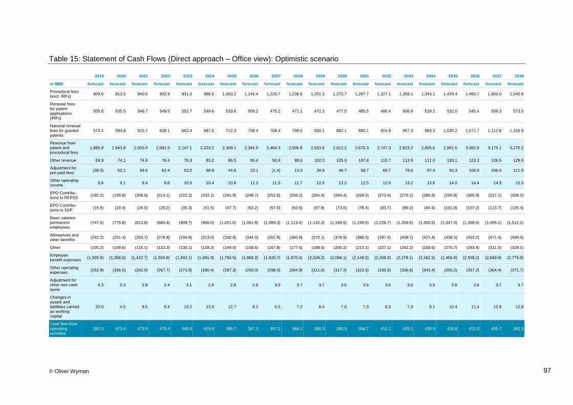
© Oliver Wyman 97

Table 15: Statement of Cash Flows (Direct approach – Office view): Optimistic scenario

2019 2020 2021 2022 2023 2024 2025 2026 2027 2028 2029 2030 2031 2032 2033 2034 2035 2036 2037 2038



809.6 813.5 840.6 902.9 931.0 986.0 1,063.2 1,142.4 1,220.7 1,236.8 1,251.3 1,272.7 1,297.7 1,327.1 1,359.1 1,393.1 1,429.4 1,465.7 1,503.0 1,540.8


505.8 535.5 546.7 549.5 552.7 549.6 533.6 509.2 475.2 471.1 472.3 477.5 485.5 495.4 506.8 519.2 532.0 545.4 559.3 573.5


570.4 594.8 615.7 639.1 663.4 687.5 712.3 739.4 768.4 799.0 830.1 862.1 893.1 924.8 957.3 993.3 1,030.2 1,071.7 1,112.8 1,155.9


1,885.9 1,943.8 2,003.0 2,091.5 2,147.1 2,223.2 2,309.1 2,391.0 2,464.3 2,506.8 2,553.6 2,612.2 2,676.3 2,747.3 2,823.2 2,905.6 2,991.6 3,082.8 3,175.1 3,270.2

Other revenue 69.9 74.1 74.8 76.4 79.3 83.2 86.5 90.4 93.9 99.0 102.0 105.0 107.8 110.7 113.9 117.0 120.1 123.3 126.6 129.9


(38.0) 52.1 58.6 62.4 53.2 58.9 44.6 23.1 (1.4) 13.0 28.8 46.7 58.7 69.7 78.6 87.4 93.3 100.9 106.0 111.9


9.6 9.1 9.4 9.8 10.0 10.4 10.8 11.2 11.5 11.7 12.0 12.2 12.5 12.9 13.2 13.6 14.0 14.4 14.9 15.3

EPO Contribu-tions to RFPSS

(195.2) (199.8) (206.0) (214.1) (222.2) (232.1) (241.9) (248.7) (252.8) (256.1) (260.4) (264.4) (269.0) (273.4) (279.1) (286.9) (295.8) (305.9) (317.1) (328.2)


(15.8) (19.4) (24.0) (29.2) (35.3) (41.5) (47.7) (53.2) (57.9) (62.6) (67.9) (73.0) (78.4) (83.7) (89.2) (94.9) (101.0) (107.2) (113.7) (120.4)


(747.5) (775.8) (813.8) (860.4) (909.7) (966.0) (1,021.0) (1,061.8) (1,089.3) (1,113.4) (1,142.3) (1,169.5) (1,199.0) (1,226.7) (1,259.5) (1,300.5) (1,347.0) (1,398.5) (1,455.1) (1,512.2)


(242.2) (251.4) (263.7) (278.8) (294.8) (313.0) (330.8) (344.0) (352.9) (360.8) (370.1) (378.9) (388.5) (397.5) (408.1) (421.4) (436.5) (453.2) (471.5) (490.0)

Other (105.2) (109.6) (115.1) (122.3) (130.1) (139.2) (149.0) (158.5) (167.8) (177.5) (188.5) (200.2) (213.1) (227.1) (242.2) (258.6) (275.7) (293.4) (311.5) (329.1)


(1,305.9) (1,356.0) (1,422.7) (1,504.8) (1,592.1) (1,691.9) (1,790.5) (1,866.3) (1,920.7) (1,970.4) (2,029.2) (2,086.1) (2,148.0) (2,208.3) (2,278.1) (2,362.3) (2,456.0) (2,558.2) (2,668.9) (2,779.9)


(253.9) (256.5) (262.0) (267.7) (273.8) (280.4) (287.3) (293.0) (298.9) (304.9) (311.0) (317.2) (323.5) (330.0) (336.6) (343.4) (350.2) (357.2) (364.4) (371.7)


4.3 2.3 2.8 2.4 3.1 2.9 2.8 2.8 3.0 3.7 3.7 3.6 3.6 3.6 3.6 3.5 3.6 3.6 3.7 3.7


20.0 4.5 9.5 9.4 13.2 13.5 12.7 8.2 5.5 7.2 8.4 7.0 7.3 6.3 7.3 9.1 10.4 11.4 12.8 12.8


392.0 473.4 473.5 479.4 440.0 419.8 388.7 367.3 357.2 366.1 368.3 383.5 394.7 412.1 425.1 430.5 426.8 421.0 405.7 392.3

© Oliver Wyman 98

2019 2020 2021 2022 2023 2024 2025 2026 2027 2028 2029 2030 2031 2032 2033 2034 2035 2036 2037 2038


Change in PPE (53.6) (53.6) (125.6) (173.6) (125.6) (77.6) (53.6) (53.6) (14.6) (14.6) (14.6) (14.6) (14.6) (14.6) (14.6) (14.6) (14.6) (14.6) (14.6) (14.6)

Change in Other financial assets

(382.5) (411.2) (338.8) (298.5) (314.6) (349.2) (350.1) (338.5) (381.9) (405.7) (424.5) (454.1) (486.2) (515.6) (541.3) (560.0) (570.2) (578.5) (577.7) (578.7)

Interest received - (2.2) (2.2) 1.1 7.2 15.1 23.7 33.2 47.4 61.1 77.9 92.8 114.2 126.6 139.6 153.3 167.5 182.0 196.6 211.3

Change in

RFPSS - - - - - - - - - - - - - - - - - - - -

Change in EPOTIF

- - - - - - - - - - - - - - - - - - - -

Other (0.8) (6.4) (6.8) (8.3) (7.0) (8.1) (8.7) (8.5) (8.1) (6.9) (7.1) (7.7) (8.0) (8.5) (8.8) (9.2) (9.5) (9.8) (10.0) (10.2)

Cash flow from

investing activities

(436.9) (473.4) (473.5) (479.4) (440.0) (419.8) (388.7) (367.3) (357.2) (366.1) (368.3) (383.5) (394.7) (412.1) (425.1) (430.5) (426.8) (421.0) (405.7) (392.3)

Cash flow from

financing activities

- - - - - - - - - - - - - - - - - - - -

Net increase/

(decrease) in cash and cash equivalents

(44.9) - - - - - - - - - - - - - - - - - - -

© Oliver Wyman 99

Table 16: Statement of Comprehensive Income: Base 2 scenario

2016 2017 2018 2019 2020 2021 2022 2023 2024 2025 2026 2027 2028 2029 2030 2031 2032 2033 2034 2035 2036 2037 2038



766.5 810.1 872.3 827.2 880.5 891.1 905.7 855.5 855.9 839.6 832.9 829.2 829.1 837.9 841.8 849.7 858.1 866.4 876.5 885.7 894.4 903.5 907.4


557.6 545.1 520.0 493.0 484.2 449.9 411.4 386.4 362.9 343.7 328.6 314.6 314.9 315.6 317.6 320.0 322.6 325.6 328.6 331.7 335.0 338.5 343.1


488.8 504.7 543.3 571.5 601.0 631.0 663.4 694.1 720.2 741.9 759.5 772.2 781.2 787.5 791.6 791.5 789.2 785.1 782.4 779.2 780.0 781.7 787.1


1,812.9 1,859.9 1,935.7 1,891.8 1,965.8 1,972.0 1,980.5 1,936.0 1,939.0 1,925.3 1,921.0 1,916.0 1,925.3 1,941.0 1,951.0 1,961.2 1,969.8 1,977.1 1,987.4 1,996.5 2,009.4 2,023.7 2,037.7

Other revenue 75.6 72.8 68.7 68.0 70.3 68.6 66.2 65.9 67.8 67.7 68.2 68.5 69.1 70.0 70.7 71.3 72.0 72.8 73.7 74.4 75.0 75.8 75.9


8.1 6.7 10.7 9.6 9.2 9.2 9.2 9.0 9.0 9.0 9.0 8.9 9.0 9.1 9.1 9.2 9.2 9.2 9.3 9.3 9.4 9.5 9.5


2.3 2.3 3.0 3.1 3.1 3.1 3.1 3.1 3.1 3.1 3.2 3.2 3.2 3.3 3.3 3.4 3.4 3.5 3.6 3.6 3.7 3.8 3.9


(642.6) (820.3) (837.2) (863.0) (721.0) (271.3) (390.6) (464.9) (462.0) (522.2) (614.9) (606.8) (594.0) (583.4) (579.7) (566.9) (553.5) (539.5) (527.3) (486.5) (461.5) (422.4) (395.9)


(691.3) (713.3) (733.9) (747.5) (755.3) (750.6) (746.6) (744.9) (752.8) (766.8) (775.0) (781.3) (785.4) (786.5) (786.2) (788.0) (787.7) (790.8) (798.7) (810.7) (824.4) (839.2) (856.1)


(218.7) (236.1) (237.8) (242.2) (244.7) (243.2) (241.9) (241.4) (243.9) (248.5) (251.1) (253.2) (254.5) (254.8) (254.7) (255.3) (255.2) (256.2) (258.8) (262.7) (267.1) (271.9) (277.4)

Healthcare and other cost of social security

(36.7) (50.8) (29.1) (31.6) (33.4) (34.7) (35.9) (37.6) (40.1) (43.6) (46.9) (50.3) (53.8) (56.9) (59.8) (62.9) (65.8) (68.8) (71.9) (75.2) (78.4) (81.6) (85.1)

Other (58.5) (58.9) (69.8) (49.6) (50.3) (50.1) (49.9) (49.6) (50.1) (50.9) (51.3) (51.7) (51.9) (52.1) (52.1) (52.2) (52.2) (52.4) (52.9) (53.7) (54.5) (55.4) (56.4)


(1,647.8) (1,879.5) (1,907.8) (1,934.0) (1,804.6) (1,349.8) (1,464.9) (1,538.4) (1,549.0) (1,632.0) (1,739.3) (1,743.2) (1,739.7) (1,733.6) (1,732.5) (1,725.3) (1,714.4) (1,707.8) (1,709.5) (1,688.7) (1,685.9) (1,670.6) (1,670.9)

Depreciation and amortization expenses

(47.2) (46.4) (63.1) (57.6) (57.5) (57.5) (63.3) (72.7) (77.3) (77.6) (75.9) (74.4) (69.8) (65.6) (61.7) (58.1) (54.9) (51.9) (49.2) (46.7) (44.5) (42.4) (40.5)


(213.2) (222.8) (252.1) (253.9) (255.2) (253.9) (252.6) (253.9) (255.7) (258.2) (261.1) (264.2) (267.6) (271.4) (275.4) (279.8) (284.6) (289.7) (295.2) (301.1) (307.2) (313.3) (319.6)

Operating result (9.4) (207.0) (204.8) (272.9) (69.0) 391.6 278.1 149.1 137.0 37.3 (74.9) (85.1) (70.5) (47.1) (35.4) (18.3) 0.5 13.1 20.0 47.3 59.9 86.4 96.0


537.6 672.1 (523.3) 300.0 (1,456.4) 599.2 551.9 508.1 392.4 402.2 342.8 355.9 366.2 385.8 398.6 416.6 426.9 436.5 447.8 460.7 462.5 473.2 472.4

© Oliver Wyman 100

2016 2017 2018 2019 2020 2021 2022 2023 2024 2025 2026 2027 2028 2029 2030 2031 2032 2033 2034 2035 2036 2037 2038


Income and gains on EPOTIF assets (net)

17.7 14.1 8.7 89.6 (346.2) 158.8 150.1 142.4 110.1 113.8 103.0 107.1 110.9 116.9 121.8 128.2 133.5 139.0 145.4 152.9 158.3 166.7 172.7


0.5 0.2 0.1 - (2.1) (2.1) (16.4) (19.9) (14.2) (12.6) (10.3) (8.1) (4.8) 0.1 5.0 11.0 16.9 23.8 31.5 39.2 46.6 55.5 63.3

Other 7.6 9.4 12.4 - - - - - - - - - - - - - - - - - - - -

Finance revenue 563.3 695.8 (502.2) 389.6 (1,804.6) 755.8 685.6 630.7 488.4 503.4 435.5 455.0 472.3 502.7 525.4 555.9 577.3 599.3 624.7 652.9 667.4 695.4 708.4

Interest costs on

defined benefit obligations

(410.7) (366.0) (358.9) (418.1) (408.7) (549.9) (524.8) (508.1) (523.3) (519.9) (530.5) (567.5) (605.2) (651.7) (703.4) (748.4) (790.4) (834.9) (889.4) (944.2) (983.4) (1,014.2) (1,039.0)

Other (3.8) (6.5) (91.3) - - - - - - - - - - - - - - - - - - - -

Finance costs (414.5) (372.4) (450.1) (418.1) (408.7) (549.9) (524.8) (508.1) (523.3) (519.9) (530.5) (567.5) (605.2) (651.7) (703.4) (748.4) (790.4) (834.9) (889.4) (944.2) (983.4) (1,014.2) (1,039.0)

Financial result 148.9 323.4 (952.3) (28.5) (2,213.4) 206.0 160.7 122.6 (34.9) (16.5) (95.0) (112.5) (132.9) (149.0) (178.0) (192.5) (213.1) (235.6) (264.7) (291.3) (316.0) (318.8) (330.6)

Profit/(loss) for

the year 139.4 116.4 (1,157.2) (301.4) (2,282.4) 597.6 438.8 271.7 102.1 20.8 (169.9) (197.6) (203.4) (196.1) (213.4) (210.9) (212.6) (222.4) (244.7) (244.1) (256.1) (232.4) (234.7)


(2,980.7) (347.0) 1,285.7 1,358.2 9,629.2 (2,425.6) (1,357.3) 362.9 (1,058.4) (2,291.1) 405.2 490.7 430.6 53.9 383.6 271.0 269.8 43.9 1.9 246.1 645.7 538.7 605.5

Total com-

prehensive income for the year

(2,841.3) (230.6) 128.5 1,056.8 7,346.8 (1,828.0) (918.5) 634.5 (956.3) (2,270.3) 235.3 293.1 227.2 (142.2) 170.2 60.2 57.2 (178.5) (242.8) 2.0 389.7 306.3 370.9

© Oliver Wyman 101

Table 17: Statement of Financial Position: Base 2 scenario

2016 2017 2018 2019 2020 2021 2022 2023 2024 2025 2026 2027 2028 2029 2030 2031 2032 2033 2034 2035 2036 2037 2038



576.8 647.2 661.8 661.0 660.3 731.6 845.0 901.1 904.6 883.9 864.8 808.3 756.4 708.8 665.1 625.0 588.2 554.5 523.5 495.1 468.9 445.0 423.0


RFPSS net assets

7,292.2 8,193.8 7,901.8 8,248.0 6,826.3 7,444.3 8,001.0 8,498.9 8,865.3 9,224.6 9,503.6 9,771.2 10,021.7 10,261.2 10,480.4 10,681.8 10,854.2 10,995.5 11,107.2 11,191.0 11,235.1 11,248.5 11,221.4


1,571.2 1,880.9 2,460.2 2,549.8 2,203.7 2,362.5 2,512.6 2,655.0 2,765.1 2,878.9 2,981.9 3,089.1 3,199.9 3,316.8 3,438.6 3,566.8 3,700.3 3,839.3 3,984.7 4,137.6 4,296.0 4,462.6 4,635.3

Home loans to staff

87.7 87.2 88.2 86.2 89.5 89.7 90.0 88.0 88.2 87.6 87.4 87.2 87.7 88.4 88.9 89.3 89.8 90.1 90.6 91.0 91.6 92.3 92.9


77.0 58.0 - 420.9 809.0 1,096.4 1,325.9 1,572.8 1,879.1 2,177.0 2,460.0 2,765.1 3,072.3 3,387.8 3,707.5 4,026.9 4,345.3 4,656.8 4,957.2 5,236.4 5,494.6 5,732.4 5,946.8

Other assets 117.3 140.1 86.8 - - - - - - - - - - - - - - - - - - - -

Non-current assets

9,771.0 11,057.7 11,237.1 12,003.5 10,627.6 11,763.5 12,813.6 13,754.2 14,540.8 15,290.2 15,935.8 16,558.8 17,176.2 17,801.5 18,419.1 19,028.8 19,616.8 20,175.4 20,702.6 21,190.7 21,626.1 22,021.0 22,359.9

Trade and other receivables

162.2 172.1 154.9 151.4 157.2 157.6 158.1 154.6 155.0 153.9 153.6 153.3 154.0 155.3 156.1 157.0 157.7 158.3 159.2 159.9 161.0 162.1 163.2

Bonds 234.9 379.2 - - - - - - - - - - - - - - - - - - - - -

Home loans to staff

7.4 7.6 7.9 7.7 8.0 8.1 8.1 7.9 7.9 7.9 7.9 7.8 7.9 7.9 8.0 8.0 8.1 8.1 8.1 8.2 8.2 8.3 8.4


318.0 87.0 58.0 - - - - - - - - - - - - - - - - - - - -

Prepaid expenses

15.1 16.6 19.3 18.9 19.6 19.7 19.7 19.3 19.3 19.2 19.2 19.1 19.2 19.4 19.5 19.6 19.7 19.8 19.9 20.0 20.1 20.2 20.4


19.6 2.3 54.9 10.0 10.0 10.0 10.0 10.0 10.0 10.0 10.0 10.0 10.0 10.0 10.0 10.0 10.0 10.0 10.0 10.0 10.0 10.0 10.0

Current assets 757.2 664.9 295.0 188.1 194.9 195.3 195.9 191.8 192.2 191.0 190.7 190.2 191.1 192.6 193.6 194.6 195.4 196.2 197.2 198.1 199.3 200.7 201.9

Total assets 10,528.2 11,722.6 11,532.2 12,191.5 10,822.5 11,958.8 13,009.5 13,946.0 14,733.1 15,481.1 16,126.5 16,749.1 17,367.3 17,994.2 18,612.7 19,223.3 19,812.3 20,371.5 20,899.8 21,388.8 21,825.4 22,221.7 22,561.8

Retained earnings

(1,734.3) (1,617.9) (2,840.5) (3,141.9) (5,424.3) (4,826.7) (4,387.9) (4,116.2) (4,014.1) (3,993.4) (4,163.2) (4,360.8) (4,564.2) (4,760.4) (4,973.7) (5,184.6) (5,397.2) (5,619.7) (5,864.4) (6,108.5) (6,364.5) (6,596.9) (6,831.6)


(8,902.0) (9,249.0) (7,963.3) (6,605.1) 3,024.1 598.5 (758.8) (395.9) (1,454.3) (3,745.4) (3,340.2) (2,849.5) (2,418.9) (2,365.0) (1,981.4) (1,710.3) (1,440.5) (1,396.6) (1,394.7) (1,148.7) (503.0) 35.7 641.3

Total equity (10,636.3) (10,866.8) (10,803.8) (9,747.0) (2,400.2) (4,228.2) (5,146.7) (4,512.1) (5,468.5) (7,738.8) (7,503.4) (7,210.3) (6,983.1) (7,125.4) (6,955.1) (6,894.9) (6,837.8) (7,016.3) (7,259.1) (7,257.1) (6,867.5) (6,561.2) (6,190.3)


19,716.5 21,087.6 20,840.8 20,574.5 11,870.1 14,895.1 16,931.4 17,288.4 19,058.7 22,095.7 22,513.3 22,844.3 23,227.3 23,986.0 24,422.9 24,960.6 25,479.5 26,202.9 26,956.9 27,425.5 27,451.5 27,519.1 27,462.9

Salary Savings

Plan obligation 58.2 79.6 86.4 - - - - - - - - - - - - - - - - - - - -


21.7 38.3 23.6 40.2 40.6 40.4 40.1 40.0 40.5 41.2 41.7 42.0 42.2 42.3 42.3 42.4 42.3 42.5 42.9 43.6 44.3 45.1 46.0

© Oliver Wyman 102

2016 2017 2018 2019 2020 2021 2022 2023 2024 2025 2026 2027 2028 2029 2030 2031 2032 2033 2034 2035 2036 2037 2038



2.4 2.4 1.9 1.8 1.9 1.9 1.9 1.9 1.9 1.8 1.8 1.8 1.8 1.9 1.9 1.9 1.9 1.9 1.9 1.9 1.9 1.9 2.0

Prepaid fees 713.8 654.3 584.4 549.2 540.7 506.6 468.8 436.4 418.6 404.4 397.3 394.0 396.4 400.5 405.3 410.4 415.7 421.2 427.4 433.5 440.7 448.5 457.7


20,512.6 21,862.3 21,537.0 21,165.7 12,453.3 15,444.0 17,442.2 17,766.7 19,519.7 22,543.1 22,954.1 23,282.1 23,667.7 24,430.7 24,872.4 25,415.2 25,939.5 26,668.6 27,429.1 27,904.4 27,938.4 28,014.6 27,968.6


129.1 155.2 165.0 162.7 164.4 163.4 162.5 162.1 163.9 166.9 168.7 170.0 171.0 171.2 171.1 171.5 171.4 172.1 173.8 176.4 179.4 182.7 186.3


182.4 219.6 201.6 203.1 204.1 203.1 202.0 203.1 204.5 206.5 208.8 211.3 214.0 217.0 220.3 223.8 227.6 231.7 236.1 240.8 245.7 250.6 255.6


4.6 3.3 1.1 1.1 1.1 1.1 1.1 1.1 1.1 1.1 1.1 1.1 1.1 1.1 1.1 1.1 1.1 1.1 1.1 1.1 1.1 1.1 1.1

Provisions 7.5 6.7 12.8 12.8 12.8 12.8 12.8 12.8 12.8 12.8 12.8 12.8 12.8 12.8 12.8 12.8 12.8 12.8 12.8 12.8 12.8 12.8 12.8

Prepaid fees 328.4 342.2 418.4 393.2 387.1 362.7 335.6 312.4 299.7 289.5 284.5 282.1 283.8 286.8 290.2 293.8 297.6 301.5 306.0 310.3 315.5 321.1 327.7


651.9 727.1 798.9 772.8 769.5 743.0 714.0 691.5 681.9 676.8 675.8 677.3 682.7 688.8 695.4 703.0 710.6 719.3 729.8 741.5 754.5 768.2 783.5


Total equity and liabilities

10,528.2 11,722.6 11,532.2 12,191.5 10,822.5 11,958.8 13,009.5 13,946.0 14,733.1 15,481.1 16,126.5 16,749.1 17,367.3 17,994.2 18,612.7 19,223.3 19,812.3 20,371.5 20,899.8 21,388.8 21,825.4 22,221.7 22,561.8

© Oliver Wyman 103

Table 18: Statement of Cash Flows (Direct approach – Office view): Base 2 scenario

2019 2020 2021 2022 2023 2024 2025 2026 2027 2028 2029 2030 2031 2032 2033 2034 2035 2036 2037 2038



827.2 880.5 891.1 905.7 855.5 855.9 839.6 832.9 829.2 829.1 837.9 841.8 849.7 858.1 866.4 876.5 885.7 894.4 903.5 907.4

Renewal fees

for patent applications (IRFs)

493.0 484.2 449.9 411.4 386.4 362.9 343.7 328.6 314.6 314.9 315.6 317.6 320.0 322.6 325.6 328.6 331.7 335.0 338.5 343.1


571.5 601.0 631.0 663.4 694.1 720.2 741.9 759.5 772.2 781.2 787.5 791.6 791.5 789.2 785.1 782.4 779.2 780.0 781.7 787.1


1,891.8 1,965.8 1,972.0 1,980.5 1,936.0 1,939.0 1,925.3 1,921.0 1,916.0 1,925.3 1,941.0 1,951.0 1,961.2 1,969.8 1,977.1 1,987.4 1,996.5 2,009.4 2,023.7 2,037.7

Other revenue 68.0 70.3 68.6 66.2 65.9 67.8 67.7 68.2 68.5 69.1 70.0 70.7 71.3 72.0 72.8 73.7 74.4 75.0 75.8 75.9


(60.4) (14.6) (58.6) (64.9) (55.6) (30.5) (24.4) (12.1) (5.8) 4.2 7.1 8.1 8.8 9.1 9.4 10.6 10.4 12.3 13.4 15.9


9.6 9.2 9.2 9.2 9.0 9.0 9.0 9.0 8.9 9.0 9.1 9.1 9.2 9.2 9.2 9.3 9.3 9.4 9.5 9.5

EPO Contribu-tions to RFPSS

(195.3) (196.6) (194.6) (192.7) (191.2) (191.9) (193.4) (193.6) (193.2) (192.3) (190.9) (189.5) (188.7) (187.7) (187.7) (189.1) (191.5) (194.6) (198.0) (201.6)


(15.8) (17.3) (18.8) (20.1) (21.8) (24.2) (27.3) (30.4) (33.8) (37.1) (40.2) (43.1) (46.2) (49.1) (52.0) (54.9) (58.0) (60.9) (63.8) (67.0)


(747.5) (755.3) (750.6) (746.6) (744.9) (752.8) (766.8) (775.0) (781.3) (785.4) (786.5) (786.2) (788.0) (787.7) (790.8) (798.7) (810.7) (824.4) (839.2) (856.1)


(242.2) (244.7) (243.2) (241.9) (241.4) (243.9) (248.5) (251.1) (253.2) (254.5) (254.8) (254.7) (255.3) (255.2) (256.2) (258.8) (262.7) (267.1) (271.9) (277.4)

Other (105.6) (109.4) (112.0) (114.3) (117.0) (121.6) (127.1) (132.9) (139.3) (146.3) (154.0) (162.2) (171.6) (181.9) (193.2) (205.5) (218.5) (232.0) (245.7) (259.1)


(1,306.4) (1,323.3) (1,319.0) (1,315.6) (1,316.4) (1,334.4) (1,363.1) (1,383.1) (1,400.6) (1,415.6) (1,426.4) (1,435.9) (1,449.9) (1,461.6) (1,480.1) (1,507.1) (1,541.3) (1,579.1) (1,618.7) (1,661.1)

Other operating

expenses (253.9) (255.2) (253.9) (252.6) (253.9) (255.7) (258.2) (261.1) (264.2) (267.6) (271.4) (275.4) (279.8) (284.6) (289.7) (295.2) (301.1) (307.2) (313.3) (319.6)


4.2 1.8 2.8 2.7 4.1 3.3 3.8 3.7 3.8 3.6 3.5 3.7 3.8 4.0 4.1 4.2 4.4 4.4 4.4 4.5


19.7 (3.4) (2.7) (2.6) 4.4 3.1 7.0 4.8 4.6 3.0 1.8 2.3 3.1 2.9 4.3 5.6 7.1 7.4 7.6 8.4

© Oliver Wyman 104

2019 2020 2021 2022 2023 2024 2025 2026 2027 2028 2029 2030 2031 2032 2033 2034 2035 2036 2037 2038


Cash flow from

operating activities

372.6 450.6 418.4 422.9 393.7 401.8 367.1 350.4 331.3 331.0 334.8 333.7 327.6 320.8 307.1 288.5 259.6 231.6 202.4 171.2

Change in PPE (53.6) (53.6) (125.6) (173.6) (125.6) (77.6) (53.6) (53.6) (14.6) (14.6) (14.6) (14.6) (14.6) (14.6) (14.6) (14.6) (14.6) (14.6) (14.6) (14.6)

Change in Other

financial assets (362.9) (388.1) (287.4) (229.5) (246.9) (306.3) (297.9) (283.0) (305.1) (307.2) (315.5) (319.6) (319.4) (318.4) (311.6) (300.4) (279.2) (258.2) (237.8) (214.4)

Interest received - (2.1) (2.1) (16.4) (19.9) (14.2) (12.6) (10.3) (8.1) (4.8) 0.1 5.0 11.0 16.9 23.8 31.5 39.2 46.6 55.5 63.3

Change in RFPSS

- - - - - - - - - - - - - - - - - - - -

Change in EPOTIF

- - - - - - - - - - - - - - - - - - - -

Other (1.0) (6.9) (3.2) (3.3) (1.3) (3.7) (2.9) (3.5) (3.5) (4.3) (4.7) (4.5) (4.6) (4.7) (4.7) (5.0) (5.0) (5.3) (5.5) (5.5)


(417.5) (450.6) (418.4) (422.9) (393.7) (401.8) (367.1) (350.4) (331.3) (331.0) (334.8) (333.7) (327.6) (320.8) (307.1) (288.5) (259.6) (231.6) (202.4) (171.2)

Cash flow from


- - - - - - - - - - - - - - - - - - - -

Net increase/


(44.9) - - - - - - - - - - - - - - - - - - -

© Oliver Wyman 105

Table 19: Statement of Comprehensive Income: Stress scenario

2016 2017 2018 2019 2020 2021 2022 2023 2024 2025 2026 2027 2028 2029 2030 2031 2032 2033 2034 2035 2036 2037 2038



766.5 810.1 872.3 834.8 877.3 853.1 831.3 830.1 817.4 793.0 781.6 756.2 750.4 748.3 744.9 741.5 736.7 732.8 731.7 728.9 729.2 729.7 730.1


557.6 545.1 520.0 487.5 474.0 441.1 412.6 382.6 355.4 331.9 311.6 294.6 290.2 286.3 283.0 280.1 278.2 277.0 276.1 275.7 275.4 275.1 274.8


488.8 504.7 543.3 572.0 602.3 631.8 661.8 689.0 713.3 732.8 747.8 757.3 762.6 764.7 763.9 758.7 750.6 740.2 730.5 719.8 712.6 706.1 703.0


1,812.9 1,859.9 1,935.7 1,894.3 1,953.5 1,926.0 1,905.8 1,901.7 1,886.1 1,857.7 1,841.0 1,808.2 1,803.1 1,799.3 1,791.9 1,780.3 1,765.5 1,750.0 1,738.3 1,724.3 1,717.1 1,710.9 1,708.0

Other revenue 75.6 72.8 68.7 67.2 69.9 64.6 62.3 63.6 63.9 63.1 63.8 61.9 61.6 62.3 62.2 61.7 61.4 61.2 61.1 60.9 61.0 61.1 61.1


8.1 6.7 10.7 9.6 9.1 9.0 8.9 8.9 8.8 8.7 8.6 8.4 8.4 8.4 8.4 8.3 8.2 8.2 8.1 8.0 8.0 8.0 8.0


2.3 2.3 3.0 3.1 3.1 3.1 3.1 3.1 3.1 3.1 3.2 3.2 3.2 3.3 3.3 3.4 3.4 3.5 3.6 3.6 3.7 3.8 3.9


(642.6) (820.3) (837.2) (863.0) (719.8) (269.9) (388.2) (460.6) (453.1) (502.1) (592.6) (586.5) (573.4) (560.3) (554.6) (540.3) (525.8) (510.1) (496.7) (460.9) (436.7) (400.2) (374.2)


(691.3) (713.3) (733.9) (747.5) (752.3) (746.1) (740.5) (734.9) (733.7) (730.7) (734.5) (740.4) (740.3) (733.6) (725.1) (719.2) (711.6) (706.8) (706.9) (712.5) (719.8) (729.3) (738.8)


(218.7) (236.1) (237.8) (242.2) (243.8) (241.8) (239.9) (238.1) (237.7) (236.8) (238.0) (239.9) (239.9) (237.7) (235.0) (233.0) (230.6) (229.0) (229.1) (230.9) (233.2) (236.3) (239.4)

Healthcare and other cost of social security

(36.7) (50.8) (29.1) (31.6) (32.9) (34.0) (35.1) (36.3) (37.5) (38.8) (41.6) (45.3) (48.4) (50.7) (52.9) (55.3) (57.5) (59.8) (62.1) (64.9) (67.5) (70.2) (73.0)

Other (58.5) (58.9) (69.8) (49.6) (50.1) (49.7) (49.3) (48.9) (48.8) (48.5) (48.7) (48.9) (48.9) (48.5) (48.0) (47.6) (47.1) (46.8) (46.8) (47.1) (47.4) (48.0) (48.5)


(1,647.8) (1,879.5) (1,907.8) (1,934.0) (1,799.0) (1,341.5) (1,453.0) (1,518.8) (1,510.9) (1,556.9) (1,655.5) (1,661.0) (1,650.8) (1,630.9) (1,615.5) (1,595.5) (1,572.7) (1,552.6) (1,541.5) (1,516.2) (1,504.5) (1,484.0) (1,473.9)


(47.2) (46.4) (63.1) (57.6) (57.5) (57.5) (63.3) (72.7) (77.3) (77.6) (75.9) (74.4) (69.8) (65.6) (61.7) (58.1) (54.9) (51.9) (49.2) (46.7) (44.5) (42.4) (40.5)


(213.2) (222.8) (252.1) (253.9) (255.2) (253.9) (252.6) (253.9) (255.7) (258.2) (261.1) (264.2) (267.6) (271.4) (275.4) (279.8) (284.6) (289.7) (295.2) (301.1) (307.2) (313.3) (319.6)

Operating result (9.4) (207.0) (204.8) (271.2) (76.1) 349.8 211.1 131.9 118.0 39.8 (75.9) (117.9) (111.9) (94.7) (86.9) (79.8) (73.6) (71.3) (74.9) (67.2) (66.3) (56.0) (53.2)


537.6 672.1 (523.3) 300.0 (1,456.3) 599.1 551.7 507.9 392.1 401.6 342.0 354.7 364.6 383.6 395.8 413.0 422.4 431.0 441.1 452.6 453.0 461.9 459.3

© Oliver Wyman 106

2016 2017 2018 2019 2020 2021 2022 2023 2024 2025 2026 2027 2028 2029 2030 2031 2032 2033 2034 2035 2036 2037 2038


Income and gains on EPOTIF assets (net)

17.7 14.1 8.7 89.6 (346.2) 158.8 150.1 142.4 110.1 113.8 103.0 107.1 110.9 116.9 121.8 128.2 133.5 139.0 145.4 152.9 158.3 166.7 172.7


0.5 0.2 0.1 - (2.0) (2.1) (15.2) (17.9) (12.8) (11.3) (9.3) (7.2) (4.3) 0.0 4.3 9.4 14.2 19.7 25.7 31.4 36.4 42.4 47.1

Other 7.6 9.4 12.4 - - - - - - - - - - - - - - - - - - - -

Finance revenue 563.3 695.8 (502.2) 389.6 (1,804.5) 755.8 686.6 632.4 489.5 504.1 435.7 454.6 471.2 500.5 521.9 550.7 570.1 589.7 612.2 636.9 647.8 671.0 679.1

Interest costs on

defined benefit obligations

(410.7) (366.0) (358.9) (418.1) (408.7) (549.8) (524.7) (507.8) (522.8) (518.9) (528.8) (565.1) (602.1) (647.6) (698.2) (742.0) (782.6) (825.5) (878.2) (930.9) (968.3) (997.3) (1,020.3)

Other (3.8) (6.5) (91.3) - - - - - - - - - - - - - - - - - - - -

Finance costs (414.5) (372.4) (450.1) (418.1) (408.7) (549.8) (524.7) (507.8) (522.8) (518.9) (528.8) (565.1) (602.1) (647.6) (698.2) (742.0) (782.6) (825.5) (878.2) (930.9) (968.3) (997.3) (1,020.3)

Financial result 148.9 323.4 (952.3) (28.5) (2,213.2) 206.0 161.9 124.7 (33.3) (14.8) (93.1) (110.5) (130.9) (147.1) (176.3) (191.3) (212.5) (235.8) (266.0) (294.1) (320.5) (326.3) (341.2)

Profit/(loss) for

the year 139.4 116.4 (1,157.2) (299.7) (2,289.3) 555.8 373.0 256.6 84.7 25.0 (169.1) (228.5) (242.8) (241.8) (263.1) (271.1) (286.1) (307.1) (340.9) (361.3) (386.9) (382.3) (394.3)


(2,980.7) (347.0) 1,285.7 1,358.2 9,628.8 (2,425.0) (1,356.5) 362.6 (1,056.8) (2,284.2) 403.4 487.9 427.5 53.0 379.5 267.4 265.5 42.3 0.9 240.6 632.0 526.1 590.3

Total com-

prehensive income for the year

(2,841.3) (230.6) 128.5 1,058.5 7,339.5 (1,869.2) (983.5) 619.2 (972.1) (2,259.2) 234.4 259.4 184.6 (188.8) 116.4 (3.7) (20.5) (264.8) (340.0) (120.7) 245.1 143.8 196.0

© Oliver Wyman 107

Table 20: Statement of Financial Position: Stress scenario

2016 2017 2018 2019 2020 2021 2022 2023 2024 2025 2026 2027 2028 2029 2030 2031 2032 2033 2034 2035 2036 2037 2038

In MN€ actual actual actual forecast forecast forecast forecast forecast forecast forecast forecast forecast forecast forecast forecast forecast forecast forecast forecast forecast forecast forecast forecast


576.8 647.2 661.8 661.0 660.3 731.6 845.0 901.1 904.6 883.9 864.8 808.3 756.4 708.8 665.1 625.0 588.2 554.5 523.5 495.1 468.9 445.0 423.0


RFPSS net

assets 7,292.2 8,193.8 7,901.8 8,248.0 6,825.7 7,442.8 7,998.1 8,493.8 8,855.9 9,207.1 9,476.5 9,733.8 9,972.3 10,197.3 10,399.1 10,580.2 10,729.4 10,844.3 10,926.2 10,977.2 10,985.2 10,959.5 10,889.5


1,571.2 1,880.9 2,460.2 2,549.8 2,203.7 2,362.5 2,512.6 2,655.0 2,765.1 2,878.9 2,981.9 3,089.1 3,199.9 3,316.8 3,438.6 3,566.8 3,700.3 3,839.3 3,984.7 4,137.6 4,296.0 4,462.6 4,635.3

Home loans to staff

87.7 87.2 88.2 86.3 88.9 87.5 86.5 86.4 85.7 84.4 83.7 82.2 82.0 81.8 81.5 81.0 80.3 79.6 79.1 78.5 78.2 77.9 77.8

Other financial

assets 77.0 58.0 - 412.5 778.8 1,016.2 1,191.5 1,420.4 1,689.4 1,960.1 2,212.3 2,458.9 2,697.3 2,935.3 3,170.4 3,394.0 3,604.1 3,796.3 3,965.3 4,098.9 4,199.1 4,263.0 4,292.8

Other assets 117.3 140.1 86.8 - - - - - - - - - - - - - - - - - - - -

Non-current assets

9,771.0 11,057.7 11,237.1 11,995.2 10,596.1 11,678.6 12,671.4 13,594.3 14,338.1 15,051.2 15,655.7 16,208.0 16,743.6 17,275.6 17,790.2 18,282.3 18,737.3 19,148.6 19,513.3 19,821.4 20,061.5 20,241.9 20,352.3

Trade and other

receivables 162.2 172.1 154.9 151.5 156.3 153.7 152.0 151.8 150.6 148.3 147.1 144.4 144.0 143.8 143.2 142.3 141.1 139.9 139.0 137.9 137.3 136.8 136.6

Bonds 234.9 379.2 - - - - - - - - - - - - - - - - - - - - -

Home loans to staff

7.4 7.6 7.9 7.8 8.0 7.9 7.8 7.8 7.7 7.6 7.5 7.4 7.4 7.4 7.3 7.3 7.2 7.2 7.1 7.1 7.0 7.0 7.0

Other financial

assets 318.0 87.0 58.0 - - - - - - - - - - - - - - - - - - - -

Prepaid expenses

15.1 16.6 19.3 18.9 19.5 19.2 19.0 18.9 18.8 18.5 18.4 18.0 18.0 17.9 17.9 17.8 17.6 17.5 17.3 17.2 17.1 17.1 17.0

Cash and cash

equivalents 19.6 2.3 54.9 10.0 10.0 10.0 10.0 10.0 10.0 10.0 10.0 10.0 10.0 10.0 10.0 10.0 10.0 10.0 10.0 10.0 10.0 10.0 10.0

Current assets 757.2 664.9 295.0 188.2 193.8 190.8 188.7 188.5 187.1 184.4 183.0 179.8 179.3 179.1 178.4 177.3 175.9 174.5 173.4 172.1 171.5 170.9 170.7

Total assets 10,528.2 11,722.6 11,532.2 12,183.4 10,789.9 11,869.4 12,860.1 13,782.8 14,525.2 15,235.6 15,838.7 16,387.9 16,923.0 17,454.7 17,968.5 18,459.6 18,913.2 19,323.0 19,686.7 19,993.5 20,233.0 20,412.9 20,522.9

Retained earnings

(1,734.3) (1,617.9) (2,840.5) (3,140.2) (5,429.5) (4,873.7) (4,500.7) (4,244.1) (4,159.4) (4,134.4) (4,303.4) (4,531.9) (4,774.7) (5,016.5) (5,279.6) (5,550.7) (5,836.8) (6,143.9) (6,484.8) (6,846.1) (7,233.0) (7,615.2) (8,009.6)


(8,902.0) (9,249.0) (7,963.3) (6,605.1) 3,023.7 598.7 (757.8) (395.2) (1,452.0) (3,736.3) (3,332.9) (2,845.0) (2,417.5) (2,364.5) (1,985.0) (1,717.6) (1,452.1) (1,409.8) (1,408.9) (1,168.2) (536.2) (10.1) 580.2

Total equity (10,636.3) (10,866.8) (10,803.8) (9,745.3) (2,405.8) (4,274.9) (5,258.5) (4,639.3) (5,611.4) (7,870.7) (7,636.3) (7,376.9) (7,192.3) (7,381.0) (7,264.6) (7,268.3) (7,288.9) (7,553.7) (7,893.7) (8,014.3) (7,769.2) (7,625.4) (7,429.4)


19,716.5 21,087.6 20,840.8 20,574.5 11,869.0 14,891.7 16,924.1 17,276.0 19,033.8 22,040.0 22,432.3 22,740.2 23,098.8 23,826.9 24,232.3 24,734.6 25,215.5 25,894.4 26,599.1 27,025.3 27,015.5 27,046.4 26,954.3


58.2 79.6 86.4 - - - - - - - - - - - - - - - - - - - -


21.7 38.3 23.6 40.2 40.4 40.1 39.8 39.5 39.4 39.3 39.5 39.8 39.8 39.4 39.0 38.7 38.3 38.0 38.0 38.3 38.7 39.2 39.7


2.4 2.4 1.9 1.8 1.9 1.8 1.8 1.8 1.8 1.8 1.8 1.7 1.7 1.7 1.7 1.7 1.7 1.7 1.7 1.6 1.6 1.6 1.6

© Oliver Wyman 108

2016 2017 2018 2019 2020 2021 2022 2023 2024 2025 2026 2027 2028 2029 2030 2031 2032 2033 2034 2035 2036 2037 2038

In MN€ actual actual actual forecast forecast forecast forecast forecast forecast forecast forecast forecast forecast forecast forecast forecast forecast forecast forecast forecast forecast forecast forecast

Prepaid fees 713.8 654.3 584.4 543.5 526.0 484.5 452.1 424.2 398.3 376.4 360.7 347.7 341.5 336.4 331.2 325.7 320.7 316.7 313.5 310.6 309.0 307.6 306.8


20,512.6 21,862.3 21,537.0 21,160.0 12,437.4 15,418.2 17,417.8 17,741.6 19,473.4 22,457.4 22,834.3 23,129.5 23,481.8 24,204.4 24,604.2 25,100.6 25,576.2 26,250.7 26,952.2 27,375.8 27,364.9 27,394.9 27,302.5

Other employee-

related liabilities 129.1 155.2 165.0 162.7 163.8 162.4 161.2 160.0 159.7 159.1 159.9 161.2 161.1 159.7 157.8 156.5 154.9 153.8 153.9 155.1 156.7 158.7 160.8


182.4 219.6 201.6 203.1 204.1 203.1 202.0 203.1 204.5 206.5 208.8 211.3 214.0 217.0 220.3 223.8 227.6 231.7 236.1 240.8 245.7 250.6 255.6

Finance lease

liabilities 4.6 3.3 1.1 1.1 1.1 1.1 1.1 1.1 1.1 1.0 1.0 1.0 1.0 1.0 1.0 1.0 1.0 1.0 1.0 1.0 1.0 1.0 1.0

Provisions 7.5 6.7 12.8 12.8 12.8 12.8 12.8 12.8 12.8 12.8 12.8 12.8 12.8 12.8 12.8 12.8 12.8 12.8 12.8 12.8 12.8 12.8 12.8

Prepaid fees 328.4 342.2 418.4 389.1 376.6 346.9 323.7 303.7 285.2 269.4 258.2 249.0 244.5 240.8 237.1 233.2 229.6 226.7 224.4 222.4 221.2 220.2 219.7


651.9 727.1 798.9 768.7 758.3 726.2 700.8 680.6 663.2 648.8 640.7 635.2 633.4 631.3 629.0 627.3 625.9 626.0 628.2 632.1 637.3 643.3 649.8


Total equity and

liabilities 10,528.2 11,722.6 11,532.2 12,183.4 10,789.9 11,869.4 12,860.1 13,782.8 14,525.2 15,235.6 15,838.7 16,387.9 16,923.0 17,454.7 17,968.5 18,459.6 18,913.2 19,323.0 19,686.7 19,993.5 20,233.0 20,412.9 20,522.9

© Oliver Wyman 109

Table 21: Statement of Cash Flows (Direct approach – Office view): Stress scenario

2019 2020 2021 2022 2023 2024 2025 2026 2027 2028 2029 2030 2031 2032 2033 2034 2035 2036 2037 2038



834.8 877.3 853.1 831.3 830.1 817.4 793.0 781.6 756.2 750.4 748.3 744.9 741.5 736.7 732.8 731.7 728.9 729.2 729.7 730.1

Renewal fees

for patent applications (IRFs)

487.5 474.0 441.1 412.6 382.6 355.4 331.9 311.6 294.6 290.2 286.3 283.0 280.1 278.2 277.0 276.1 275.7 275.4 275.1 274.8


572.0 602.3 631.8 661.8 689.0 713.3 732.8 747.8 757.3 762.6 764.7 763.9 758.7 750.6 740.2 730.5 719.8 712.6 706.1 703.0

Renewal fees for patent applications

1,894.3 1,953.5 1,926.0 1,905.8 1,901.7 1,886.1 1,857.7 1,841.0 1,808.2 1,803.1 1,799.3 1,791.9 1,780.3 1,765.5 1,750.0 1,738.3 1,724.3 1,717.1 1,710.9 1,708.0

Procedural fees related to the Patent Grant Process

67.2 69.9 64.6 62.3 63.6 63.9 63.1 63.8 61.9 61.6 62.3 62.2 61.7 61.4 61.2 61.1 60.9 61.0 61.1 61.1

National renewal

fees for granted patents

(70.3) (30.0) (71.2) (55.6) (47.9) (44.4) (37.7) (26.9) (22.2) (10.8) (8.7) (8.9) (9.4) (8.5) (6.9) (5.5) (4.9) (2.8) (2.4) (1.4)

Revenue from

patent and procedural fees

9.6 9.1 9.0 8.9 8.9 8.8 8.7 8.6 8.4 8.4 8.4 8.4 8.3 8.2 8.2 8.1 8.0 8.0 8.0 8.0

Other revenue 487.5 474.0 441.1 412.6 382.6 355.4 331.9 311.6 294.6 290.2 286.3 283.0 280.1 278.2 277.0 276.1 275.7 275.4 275.1 274.8

Adjustment for

pre-paid fees 834.8 877.3 853.1 831.3 830.1 817.4 793.0 781.6 756.2 750.4 748.3 744.9 741.5 736.7 732.8 731.7 728.9 729.2 729.7 730.1


572.0 602.3 631.8 661.8 689.0 713.3 732.8 747.8 757.3 762.6 764.7 763.9 758.7 750.6 740.2 730.5 719.8 712.6 706.1 703.0

EPO Contribu-

ions to RFPSS (195.3) (196.2) (193.9) (191.8) (189.7) (189.0) (187.9) (187.2) (186.5) (184.7) (181.9) (178.9) (176.6) (174.1) (172.6) (172.5) (173.7) (175.5) (177.9) (180.1)


(15.8) (17.0) (18.2) (19.4) (20.7) (22.0) (23.3) (26.1) (29.6) (32.7) (35.1) (37.5) (40.1) (42.4) (44.8) (47.1) (49.7) (52.2) (54.7) (57.3)


(747.5) (752.3) (746.1) (740.5) (734.9) (733.7) (730.7) (734.5) (740.4) (740.3) (733.6) (725.1) (719.2) (711.6) (706.8) (706.9) (712.5) (719.8) (729.3) (738.8)

Allowances and

other benefits (242.2) (243.8) (241.8) (239.9) (238.1) (237.7) (236.8) (238.0) (239.9) (239.9) (237.7) (235.0) (233.0) (230.6) (229.0) (229.1) (230.9) (233.2) (236.3) (239.4)

Other (105.6) (109.2) (111.5) (113.7) (116.3) (120.3) (124.7) (130.2) (136.5) (143.2) (150.4) (158.2) (167.0) (176.8) (187.6) (199.4) (211.9) (225.0) (238.3) (251.2)


(1,306.4) (1,318.4) (1,311.5) (1,305.4) (1,299.8) (1,302.7) (1,303.4) (1,316.0) (1,332.9) (1,340.7) (1,338.9) (1,334.7) (1,336.0) (1,335.6) (1,340.9) (1,355.0) (1,378.7) (1,405.6) (1,436.6) (1,466.7)


(253.9) (255.2) (253.9) (252.6) (253.9) (255.7) (258.2) (261.1) (264.2) (267.6) (271.4) (275.4) (279.8) (284.6) (289.7) (295.2) (301.1) (307.2) (313.3) (319.6)


4.2 2.1 3.5 3.3 3.3 3.7 4.1 3.9 4.3 3.9 3.9 4.1 4.3 4.5 4.6 4.6 4.8 4.8 4.8 4.9

© Oliver Wyman 110

2019 2020 2021 2022 2023 2024 2025 2026 2027 2028 2029 2030 2031 2032 2033 2034 2035 2036 2037 2038



19.5 (3.0) 0.1 (0.6) (0.3) 2.4 3.8 4.7 7.1 3.2 1.5 1.6 3.0 3.0 4.2 5.5 7.5 7.4 8.1 7.8

Cash flow from

operating activities

364.3 428.1 366.6 366.1 375.6 362.1 337.9 318.0 270.6 260.9 256.3 249.1 232.4 214.0 190.7 161.9 120.8 82.7 40.6 2.1

Change in PPE (53.6) (53.6) (125.6) (173.6) (125.6) (77.6) (53.6) (53.6) (14.6) (14.6) (14.6) (14.6) (14.6) (14.6) (14.6) (14.6) (14.6) (14.6) (14.6) (14.6)

Change in Other

financial assets (354.5) (366.3) (237.4) (175.3) (228.9) (268.9) (270.7) (252.2) (246.6) (238.4) (238.0) (235.1) (223.6) (210.1) (192.1) (169.1) (133.6) (100.2) (63.9) (29.8)

Interest received - (2.0) (2.1) (15.2) (17.9) (12.8) (11.3) (9.3) (7.2) (4.3) 0.0 4.3 9.4 14.2 19.7 25.7 31.4 36.4 42.4 47.1

Change in RFPSS

- - - - - - - - - - - - - - - - - - - -

Change in EPOTIF

- - - - - - - - - - - - - - - - - - - -

Other (1.0) (6.2) (1.5) (1.9) (3.2) (2.7) (2.2) (2.9) (2.1) (3.6) (3.8) (3.7) (3.6) (3.5) (3.6) (3.9) (3.9) (4.4) (4.5) (4.7)


(409.2) (428.1) (366.6) (366.1) (375.6) (362.1) (337.9) (318.0) (270.6) (260.9) (256.3) (249.1) (232.4) (214.0) (190.7) (161.9) (120.8) (82.7) (40.6) (2.1)

Cash flow from


- - - - - - - - - - - - - - - - - - - -

Net increase/


(44.9) - - - - - - - - - - - - - - - - - - -

© Oliver Wyman 111

Appendix B. Assumptions in the financial model

Table 22: Assumptions in the financial model

Topic Assumption Description Value Key variables influenced Source

Workforce Average retirement age

Average retirement at which all staff is assumed to retire

61 years, constant over time Lower bound for examiner workforce

2014-2018 average value (rounded to full years), HR statistics

Examiner new hires

Number of newly hired examiners per annum

Number of new hires is calculated such that stock is in line with Early Certainty criteria – see section 3.6.1

Total number of examiners Modelling approach

Formality officers’ new hires

Number of newly hired formality officers per annum

Total number of formality examiners are assumed to vary in due proportion (as of 2018) of examiners

Total number of formality officers

Assumption as agreed with the EPO

Other staff new hires

Number of newly hired employees that are not examiners or formality officers

The total number of other staff is assumed as constant over time

Total number of other staff Assumption as agreed with the EPO

Additional leaves

Number of employees leaving due to reasons other than retirement

There are no leaves assumed other than retirements

Total number of examiners/ formality officers/ other staff


Minimum replacement ratio

Minimum share of retiring employees that need to be replaced by new hires

0% Total workforce Assumption as agreed with the EPO

Man-years Number of examiner man-years available during the year

Average of headcount beginning and end of year

Time available for SEO production

Modelling approach

© Oliver Wyman 112


SEO time per examiner (in days)

Total time available for SEO activities is determined based on available examiner man-years and the following components:

Gross capacity relative to man-years, unpaid capacity and leave, sickness (examiner population), section II investment, initial training, section III investment, section I investment other than opposition.

Adjustments are made for reduced productivity of new hires in addition to initial training requirements as well as workforce reskilling

Projected based on 2016-2018 average values, constant over time

SEO production capacity Management Dashboard 2016-2018, DG1 business services

Initial training of new hires

FTE days required for initial training of new hires including coaching days

First year: 65 days, second year 37 days

SEO time DG1 business services

Percentage JG1-4 in Other employees

Percentage of employees that are not examiners or formality officers (“other staff”) belonging to job groups 1-4

53.87%, constant over time Salaries for employee group "other staff"; basic salaries permanent employees, pension liabilities

Based on 2018 actuals, HR statistics

© Oliver Wyman 113


Patent Grant Process

Time per product

Time required for search, examination and opposition

2018: search: 1.98, examination: 1.50 days, opposition: 7.35 days (calibrated to 2018 actuals).

Increase of 3% until 2022 then constant

SEO production possible with given workforce per annum

2018 actuals, DG1 business services, Management Dashboard 2018, assumption as agreed with the EPO

Target and minimum stock

Target stock is defined in line with Early Certainty criteria (EPO case view). A convergence process is assumed until 2024 (“soft landing”) after which it equals minimum stock.

Minimum stock that cannot be undershot is assumed in line with Early Certainty criteria constant over time.

• 5 months of total search production output of the examiner workforce based on time per product assumed in a given year – see section 3.6.1

• 25 months of total examination production output of the examiner workforce based on time per product assumed in a given year

• No target and minimum stock set for opposition as stock not explicitly modelled

Search and examination production, search and examination cases completed


Search/ examination ratio (S/E ratio)

Ratio of searches conducted per examination per annum

Optimized in financial model with respect to target stock achievement

Search and examination production, search and examination cases completed

Modelling approach

Cases completed without production

Share of cases that is completed without examiner production due to withdrawal of application, etc.

• 3.00% on top of search production

• 5.27% on top of examination production

Search and examination cases completed

2016-2018 average values, 2016,2017: MTBP 2018 Scenario V3, 2018: Management Dashboard 2018

© Oliver Wyman 114


Production split search

Split assumed between search products

• Euro-direct

• Euro-PCT international phase

• Euro-PCT supplementary phase

• Others"

Split between products assumed to reflect split of incoming workload in each year

Procedural fee income Modelling approach

Product split within search stock and examination stock

Split between product types in the stock of search and the stock of examination

No differentiation assumed

Procedural fee income Modelling approach

Incoming workload European examinations

Percentage of searches, excluding searches for national offices, resulting in European examinations

67.62%, constant over time Incoming workload European examinations

2016-2018 average, 2016, 2017: MTBP 2018 Scenario V3, 2018: Management Dashboard 2018

Incoming workload PCT Ch II

Percentage of PCT International resulting in PCT CH II examinations

9.84%, constant over time Incoming workload PCT Ch II


Patents published

Percentage of European examinations resulting in published patents

65.36%, constant over time EPPU02 (Published Patents)


Incoming workload PCT searches

Share of Euro-PCT international searches of Euro-PCT searches incoming workload

62.91%, constant over time Euro-PCT international phase search cases completed; Euro-PCT supplementary search cases completed

2018 actuals, Management Dashboard 2018

© Oliver Wyman 115


Product split examination

Share of European examination cases completed in total examination cases completed

95.88%, constant over time European examination cases completed; PCT chapter II examination cases completed

2018 actuals, Management Dashboard 2018

Income statement

Procedural fees Procedural fees payable per product

Calculation based on 2018 revenue per product type divided by production per product type in 2018 (Procedural fees for examination and grant – EPC and Euro-PCT are interpolated based on fee structure from 2019 onwards to account for one-off effects in 2018)

Revenue - procedural fees 2018 actuals, IFRS financial statements 2018, Management Dashboard 2018

Increase of procedural fees

Increase of all procedural fees per annum

No increase assumed except one-off fee adjustment of 4% in 2020

Revenue - procedural fees Assumption as agreed with the EPO

Amount of internal renewal fees paying cases

Number of IRF paying cases in relation to total pending cases

Number of cases paying IRF modelled in relation to number of pending cases: 86.62%, constant over time

Revenue - internal renewal fees

2018 actuals, Finance statistics, MTBP 2018 Scenario V3

Internal renewal fees

Internal renewal fees payable per annum per case split by ordinal years

Actual fee structure as of 2018, constant over time


2018 actuals, Finance statistics

Internal renewal fees calibration factor

Factor to calibrate bottom-up calculated IRFs to historical values in IFRS income statement

+2.42%, constant over time (related to refunds, interest to late payments and other)


2016-2018 actuals, IFRS financial statements 2017, 2018

Increase of internal renewal fees

Increase of internal renewal fees per annum

No increase assumed except one-off fee adjustment of 4% in 2020



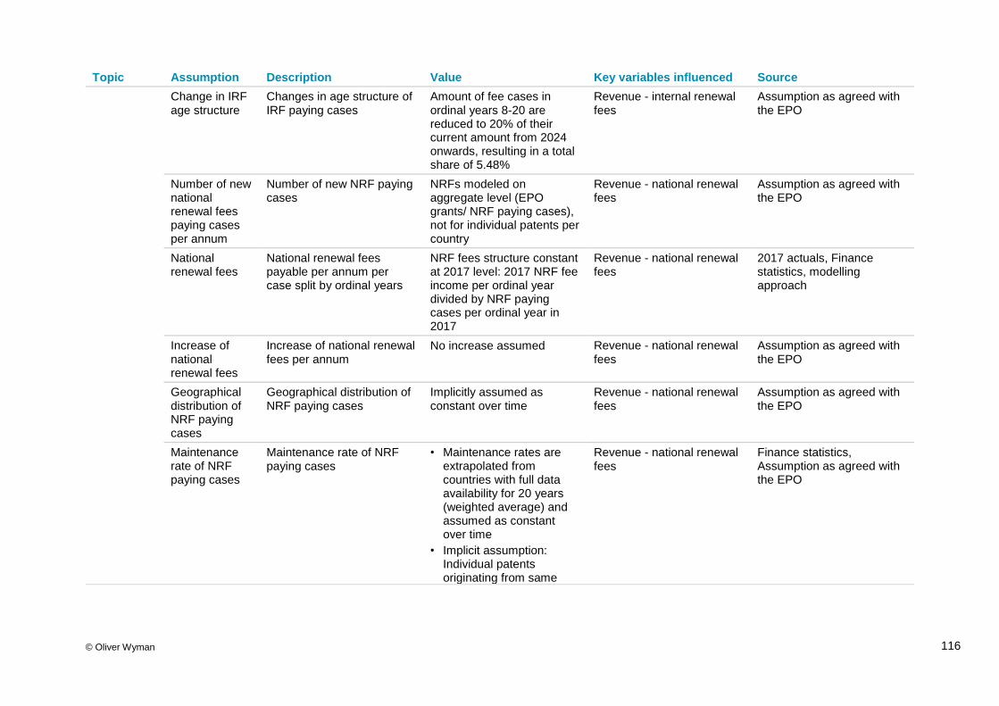
© Oliver Wyman 116


Change in IRF age structure

Changes in age structure of IRF paying cases

Amount of fee cases in ordinal years 8-20 are reduced to 20% of their current amount from 2024 onwards, resulting in a total share of 5.48%



Number of new national renewal fees paying cases per annum

Number of new NRF paying cases

NRFs modeled on aggregate level (EPO grants/ NRF paying cases), not for individual patents per country

Revenue - national renewal fees


National renewal fees

National renewal fees payable per annum per case split by ordinal years

NRF fees structure constant at 2017 level: 2017 NRF fee income per ordinal year divided by NRF paying cases per ordinal year in 2017


2017 actuals, Finance statistics, modelling approach

Increase of national renewal fees

Increase of national renewal fees per annum

No increase assumed Revenue - national renewal fees


Geographical distribution of NRF paying cases

Geographical distribution of NRF paying cases

Implicitly assumed as constant over time



Maintenance rate of NRF paying cases

Maintenance rate of NRF paying cases

• Maintenance rates are extrapolated from countries with full data availability for 20 years (weighted average) and assumed as constant over time

• Implicit assumption: Individual patents originating from same


Finance statistics, Assumption as agreed with the EPO

© Oliver Wyman 117

Topic Assumption Description Value Key variables influenced Source EPO grant have same lifetime in all countries in which they are validated

Cases paying NRF in year of grant

Share of patents granted that pay NRF in the year the patent was granted

44.00% Revenue - national renewal fees

Finance statistics

Validation in member states

Share of patents granted that are validated in at least one member state

96.74% Revenue - national renewal fees

Finance statistics

Change in NRF age structure

Changes in the age structure of new NRF paying cases

Share of new fee cases in ordinal years 8-20 is reduced to 20% of their current share. This is assumed as a gradual process over time completed in 2024.



Patents validated per grant

Number of patents validated in different countries stemming from one EPO grant

Implicitly assumed as constant as of 2017



National renewal fees calibration factor

Factor to calibrate bottom-up calculated NRFs to historical values in IFRS income statement

+0.54%, constant over time (related to accruals, minimum fees and others)


2016-2018 actuals, IFRS financial statements 2017, 2018

Patent information services and products Administrative fees

Modelling of IFRS income statement positions

Growth in line with revenue Revenue Modelling approach

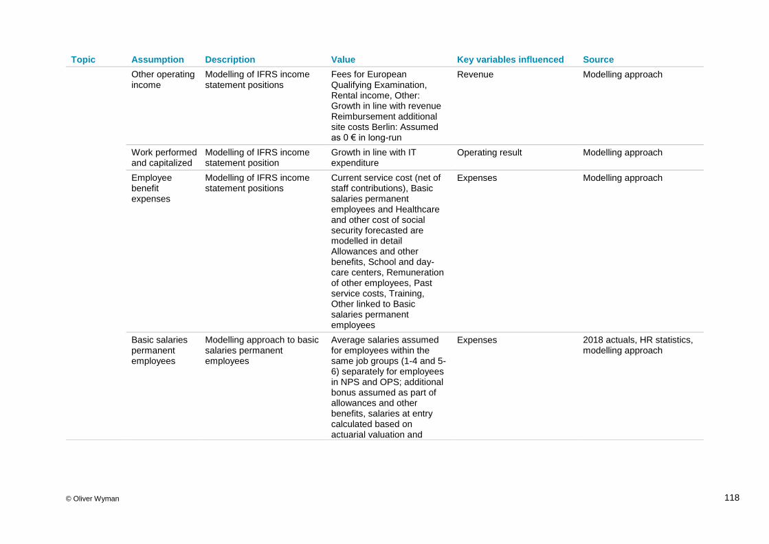
© Oliver Wyman 118




Fees for European Qualifying Examination, Rental income, Other: Growth in line with revenue Reimbursement additional site costs Berlin: Assumed as 0 € in long-run

Revenue Modelling approach


Modelling of IFRS income statement position

Growth in line with IT expenditure

Operating result Modelling approach



Current service cost (net of staff contributions), Basic salaries permanent employees and Healthcare and other cost of social security forecasted are modelled in detail Allowances and other benefits, School and day-care centers, Remuneration of other employees, Past service costs, Training, Other linked to Basic salaries permanent employees

Expenses Modelling approach


Modelling approach to basic salaries permanent employees

Average salaries assumed for employees within the same job groups (1-4 and 5-6) separately for employees in NPS and OPS; additional bonus assumed as part of allowances and other benefits, salaries at entry calculated based on actuarial valuation and

Expenses 2018 actuals, HR statistics, modelling approach

© Oliver Wyman 119

Topic Assumption Description Value Key variables influenced Source hence actual observation. See section 3.7.1 for details

Growth of average salaries

Yearly growth of average salaries

Yearly adjustment of average salaries with career progression factor of 1.74% and inflation + 0.5%. Explicit consideration of impact of new hire on average salary. See section 3.7.1 for details

Expenses Finance statistics, HR statistics

Basic salaries permanent employee’s calibration factor

Factor to calibrate bottom-up calculated basic salaries permanent employees to historical values in IFRS income statement

-1.27% (related to leaves/ recruitment during year)

Expenses 2016-2018 actuals, IFRS financial statements 2017, 2018


Modelling of IFRS income statement position

8.22% of PPE (previous year)

Expenses 2017-2018 actuals, 2018 IFRS financial statements



Growth in line with inflation Expenses Modelling approach

Balance sheet

Capital expenditure

Capital expenditure assumed in the 20-year time horizon of the Financial Study

600 MN€ are assumed between 2019-2026; thereof 20% additional building costs distributed equally over time; remaining amount distributed as follows: 2019: 5.00%, 2020: 5.00%, 2021: 20.00%, 2022: 30.00%, 2023: 20.00%,2024: 10.00%,

Non-current assets Interview with PD General Administration (EPO)

© Oliver Wyman 120

Topic Assumption Description Value Key variables influenced Source 2025: 5.00%, 2026: 5.00% (assumption)

Property plant and equipment

Modelling of IFRS balance sheet position

See Capital Expenditure and depreciation and amortization expenses

Non-current assets Modelling approach

Intangible assets


Growth in line with IT expenditure


Home loans to staff


Growth in line with revenue Current/ non-current assets Modelling approach

Other financial assets - current assets


Growth in line with revenue Current assets Modelling approach

Other financial assets - non-current assets


All excess cash flow assumed to be deposited into this position; 1-year government bond interest rates assumed as return for this position


Trade and other receivables, prepaid expenses


Growth in line with revenue Current assets Modelling approach



Cash and cash equivalents are assumed to be 10 MN€ from 2019-2038 as excess liquidity will be treated as other financial assets

Current assets Modelling approach

© Oliver Wyman 121


Adjustment of prepaid fees

Adjustment of prepaid fees due to increased productivity

Prepaid fees are assumed to change in line with stock development and revenue growth

Current/ non-current liabilities

Modelling approach



Not modelled from 2019-2038 as it is neutral regarding the balance sheet

Non-current liabilities Modelling approach

Trade and other payables, Finance lease liabilities


Growth in line with other operating expenses

Current liabilities Modelling approach

Provisions Modelling of IFRS balance sheet position

Assumed as constant from 2018 on




Growth in line with basic salaries permanent employees


Cash flow statement

Cash receipts from customers

Modelling of cash flow statement positions related to cash receipts from applicants

Based on revenue and other operating income as calculated in IFRS incomes statement adjusted for changes in pre-paid fees

Cash receipts from customers

Modelling approach

Cash paid to employees

Modelling of cash flow statement positions related to cash paid to employees

Based on Employee benefit expenses as calculated in IFRS incomes statement with the following adjustments:

• Current service costs are excluded

• Additional consideration of EPO contributions to RFPSS and SSP

Cash paid to employees Modelling approach

© Oliver Wyman 122


• Adjustment for tax allowance, family allowance and death

• Adjustment for other non-cash items

Cash paid to suppliers

Modelling of cash flow statement positions related to cash paid to suppliers

Based on other operating expenses as calculated in IFRS incomes statement with additional consideration of changes in assets and liabilities carried as working capital

Cash paid to suppliers Modelling approach


Modelling of cash flow statement positions related to investing activities

Modelled based on changes in respective balance sheet items


Modelling approach


Modelling of cash flow statement positions related to financing activities

No cash flow from financing activities assumed from 2019 onwards


Modelling approach

Employee benefits

Longevity

Increased life expectancy of the population

+2 years in the Base 1, Base 2 and Stress scenario compared to 2017 IFRS valuation

Employee benefit liabilities, Service cost, cash flow (impact on tax adjustment payments) and RFPSS assets


Service cost

Benefits EPO employees accrue within one year

Real discount rate sensitive projection depending on closed group and new hires

Defined-benefit obligation

Cash-flow projections are provided by the International Service for Remunerations and Pensions (ISRP) as of December 31st, 2017 for the next 100 years, an assumption for new entrants from the Actuarial Valuation

© Oliver Wyman 123

Topic Assumption Description Value Key variables influenced Source of 2017 and Mercer actuarial estimates

New hires Assumption for key actuarial parameters for new hires

Age, gender and grade distribution for new hires

Service Cost for new hires Actuarial valuation as of December 31st, 2017 provided by International Service for Remunerations and Pensions (ISRP)

Payments

Projected benefit payments based on the current population. The assumption for new hires is that there are no payments within the projection horizon of 20 years

Real Benefit Payments almost triple over next 20 years (2018: 280 MN€ and 2038: 787 MN€)

Defined-benefit obligation and asset volume of RFPSS (as assumed to be activated)

Cash-flow projections are as of December 31st, 2017 for the next 100 years provided by International Service for Remunerations and Pensions (ISRP)

RFPSS and EPOTIF

Contributions

Contribution rates for pensions and LTC depend on pensionable salary and are set by an independent Actuarial Advisory Group. For health, CA/D 7/10 to the basic salaries, pensions and invalidity is applied.

OPS: 29.4% NPS: 24.9% with 4.5% of salary paid into a defined-contribution component (Salary Savings Plan: SSP) LTC: 1.5%

Asset volume of RFPSS, no contributions to EPOTIF are assumed.

Actuarial Valuation 2016 and CA/D 7/10

Income and Gains

Allocations are aggregated to fixed income assets (which are sensitive to the corporate bond yields) and growth assets (which are sensitive to the European equity market return)

Sensitivity to interest rate measured in Duration (in years):

• RFPSS: 4.9

• EPOTIF: 6.2

Sensitivity to European equity market sensitivity measured in Equity beta:

• RFPSS: 0.5

• EPOTIF: 0.8

Asset volume of RFPSS and EPOTIF

Mercer analysis

© Oliver Wyman 124

Appendix C. PESTEL analysis of exogeneous drivers of the EPO’s financial situation

Political

The greatest political risks (apart from worst case scenarios like armed conflicts, which are not considered here) are related to the future of economic globalization and international trade67. Overall, the era of globalization with strong catch-up by emerging economies, particularly in Asia, has been highly beneficial to the global macroeconomic environment, multinationals’ profitability and R&D investment, and resulting demand for EPO services. In a recent survey on this topic, The Economist summarizes global developments as follows:68 Whereas the period 1990-2010 can be considered as “the global era of globalization”, with declining trade barriers, soaring trade and company profits and global investment, “globalization has slowed from light speed to a snail’s pace in the past decade. Cross-border investment, trade, bank loans, have all been shrinking or stagnating relative to world GDP. Globalization has given way to a new era of sluggishness” dubbed “slowbalization”. The effect on the EPO has been visible as well. Figure 59 illustrates how the different eras of globalization/ slowbalization had a different impact on the demand for EPO services. Whereas the growth rate of total applications between 1990 and 2010 was 4.9% p.a., between 2017 and 2010, it was only 1.3% p.a.

Figure 59: Growth in EPO Applications 1990-201769

Source: IP5 statistics and EPO

According to economic and political observers, “slowbalization” might still become something worse. Fears of a global trade war have increased lately, especially with the US administration’s hard stance in relation to China70 and the EU. While a trade conflict will most likely lower global economic activity and R&D investment, the direct impact on demand for EPO services is ambiguous: on the one hand, a trade war could even deteriorate into outright protectionist measures, such as the emergence of several regionalized technical standards, so more inventions would have to be made in parallel, each under a different standard.71 On the other hand, firms’ desire to protect inventions in foreign markets could decrease when these markets are made less accessible and profitable by tariffs or other

67 World Economic Forum Global Risks report 2019 68 The Economist: Briefing on Slowbalization, January 26th 2019 edition.

70 https://foreignpolicy.com/gt-essay/understanding-trumps-trade-war-china-trans-pacific-nato/, accessed

February 18 2019. 71 Opinion offered in the Round Table on Forecasting session, 31 January 2019.

50 000

90 000

130 000

170 000

210 000

19

90

19

91

19

92

19

93

19

94

19

95

19

96

19

97

19

98

19

99

20

00

20

01

20

02

20

03

20

04

20

05

20

06

20

07

20

08

20

09

20

10

20

11

20

12

20

13

20

14

20

15

20

16

20

17

2010-20171.3% p.a.

1990-2010: 4.9% p.a.

https://foreignpolicy.com/gt-essay/understanding-trumps-trade-war-china-trans-pacific-nato/

© Oliver Wyman 125

trade obstacles. As an example for this ambiguity, consider that “Chinese investment into Europe and America fell by 73% in 2018”, whereas “in Asia and Europe most trade is already intra-regional, and the share has risen since 2011”.72 Overall, trade friction and rising trade barriers are likely to have a negative impact on demand for EPO services.

The second most important geopolitical megatrend that affects the EPO is the emergence of China as an R&D giant and international patent holder.73 This role is being driven by the ambitions of the Chinese government to establish China as a global science and technology hub with a strong focus on applied sciences deemed relevant for future global growth. The key objective is not only to become independent from Western innovations, but also to become a global technology leader in order to sustain its export-led growth.

So far, China has been extremely successful in this regard. In the last 20 years, China’s R&D expenses have grown from virtually nil to the level of the US and Europe. It now has three times the number of scientists and engineers than the EU. This politically stimulated R&D catch-up also translates into patenting. As Figure 60 below illustrates, China is now by far the most important patenting country in the world. So far, the translation into EPO patent applications has been limited because of an initial focus on China domestic patent protection. However, the Japanese and Korean examples show it is most likely only a matter of time until Chinese firms, after a phase of domestic consolidation, will want to conquer market shares in the EU and seek IP protection in Europe (as was the case for Huawei).74 Over the next 20 years, this “China catch-up process” could be a strong stimulator of demand growth for EPO services. 75 However, given current trade tensions, there is a significant risk that this catch-up will not materialize. There is even the risk (under rising regional blocks and the shifting of the world’s economic center of gravity towards Asia), that the rise of China might become detrimental for the demand for EPO services, especially in case a demographically and economically stagnating Europe becomes less attractive for non-European multinationals.

72 The Economist: Slowbalization, January 26th 2019 edition. 73 For a concise overview on this megatrend, read The Economist: Red moon rising – Will China dominate

science? The great experiment, January 12th 2019 edition. 74 In 2017, Huawei already was the most important EPO applicant. The Korean firms LG and Samsung were on

place three and four. 75 Overall expert consensus in the EPO‘s Round Table on Forecasting session, 31 January 2019.

© Oliver Wyman 126

Figure 60: International patent filings by applicant’s country of residence

Source: WIPO statistics

In comparison, the Brexit (and the possibility of other exits from the European Union) is not expected to affect patenting activity at the level of the EPO beyond the effects already considered in GDP forecasts, as it seems unlikely that - despite Brexit - the UK would withdraw from the European Patent Convention. 76

Economic

Based on empirical evidence, it is assumed that patenting demand primarily depends on global economic activity, i.e. real (inflation-corrected) GDP and R&D.77 Capital market developments are already considered in GDP forecasts and should not be considered twice for demand forecasting. This is also true for exchange rate developments, which need to be considered the outcome, not the cause, of international trade developments. In the four scenarios used in this Study, certain macroeconomic scenarios impacting GDP development to account for this uncertainty are applied.78 While the R&D-to-GDP ratio is assumed to remain stable for most advanced economies, some variation for China is considered. In line with general market expectations,79 it is expected that China’s current R&D to GDP ratio (slightly above 2% and above the EU-average) could rise towards current Korean levels (above 4% of GDP).

Sociocultural

Sociocultural events are assumed to have no impact on the demand for EPO services other than beyond any effects already covered by political and macroeconomic factors. Demographic ageing is considered the most impactful sociocultural phenomenon in Europe. Per se, this should be detrimental to R&D activities as societies become less innovative, more conservative and risk averse and the costs of preserving the social security system and keeping public debt sustainable will drag on companies’ profits after tax.

76 https://www.epo.org/news-issues/news/2018/20180125.html. 77 Such a relationship has been applied by e.g. Hingley, P., and W. G. Park, Do Business Cycles Affect

Patenting? Evidence from European Patent Office Filings, Technological Forecasting & Social Change 116 (2017) 76–86 or by de Rassenfosse and van Pottelsberghe de la Potterie, On the Price Elasticity of Demand for Patents, Oxford Bulletin of Economics and Statistics, Vol. 74, No. 1, p. 58-77.

78 In the general modelling of the development of the EPO’s overall financial position, the overall macroeconomic environment assumed for the different scenarios is consistently translated into other relevant macroeconomic variables (inflation, interest rates, fiancial market developments).

79 See The Economist: Red moon rising – Will China dominate science? The great experiment, January 12th 2019 edition.

0

400.000

800.000

1.200.000

1.600.000

2008 2009 2010 2011 2012 2013 2014 2015 2016 2017

China US Germany Japan Korea

https://www.epo.org/news-issues/news/2018/20180125.html

© Oliver Wyman 127

Demographic ageing has been considered as an external driver for pension modelling (i.e. life expectancy of pensioners).

Technological

Digitization and Artificial Intelligence (AI) are considered the most important technological megatrends as they potentially impact all industries80. They may have a strong, but as yet uncertain, impact on overall patent demand81: on the one hand, a large increase in interest in invention protection and patenting demand may be observed. Major technological transformations may generate many new R&D activities and innovations. However, many new IP elements that are software based may not be patentable. As software has a very short economic lifetime, the new digital components of patent applications might shorten the average lifetime of innovations, making the application for patent protection less attractive. The large uncertainty regarding the overall impact of technology has been considered in the scenario analysis through a strengthening or weakening of the established GDP to patent applications link observed in the past.

Environmental

Limiting climate change and the protection of the environment has triggered a considerable amount of innovation in climate change mitigation technology.82 After experiencing a peak in 2012, the number of clean energy related patents (solar, wind, geothermal energy and fuel cell technology) however, has decreased since then and only represents a negligible share (approximately 1%) of total patenting activity.83 It is therefore assumed that environmental influences will only have a limited effect on patenting demand or be indirect, so that the impact will be already be seen in GDP or as part of overall technology megatrends.84

Legal

Two potential issues need to be considered in more detail: the future attractiveness of the EPO in competition with other patent offices and the introduction of the European Unitary Patent (UP).

Looking at patentees’ behavior, several factors influence the decision to use a particular patent office. Besides the nature of the invention and the markets in which the invention can be exploited, the quality of a patent office’s services and price have been shown to affect the propensity to patent.85 While the laxity of patent offices and lower examination standards have been put forward by economic literature as the key drivers for boosting the massive growth in filings that were experienced at some offices in the past,86 the superior quality of

80 BRINK: 73 Percent of Executives See Disruption on the Horizon—and It’s Making Workers Nervous, 26

February 2019. 81 Opinion offered at the EPO Round Table on Forecasting session, 31 January 2019. 82 EPO, Climate change mitigation technologies in Europe – evidence from patent and economic data, available

at https://www.epo.org/news-issues/technology/sustainable-technologies/clean-energy/europe.html.

83 WIPO, World Intellectual Property Indicators 2018, pp. 24 and 30, available at https://www.wipo.int/edocs/pubdocs/en/wipo_pub_941_2018.pdf.

84 Opinion offered at the Round Table on Forecasting session, 31 January 2019.

85 van Pottelsberghe de la Potterie, B., The Quality Factor in Patent Systems, in: Industrial and Corporate Change, Vol. 20, pp. 1755-1793.

86 See van Pottelsberghe de la Potterie, B., The Quality Factor in Patent Systems, in: Industrial and Corporate Change, Vol. 20, pp. 1755-1793, and de Rassenfosse, G., and B. van Pottelsberghe de la Potterie, On the Price Elasticity of Demand for Patents, in: Oxford Bulltin of Economics and Statistics (2012), Vol. 74, p. 60 for further references.

© Oliver Wyman 128

the examination process on the other hand appears to be an incentive to file to a particular office such as the EPO.87

With respect to the role of patent fees on the demand for patents, economic literature reveals an inelastic demand for patents with a fee elasticity typically below unity88. This does

not support the alternative view that strong competition of the EPO with other patent offices presents a barrier to further increasing pricing (where international benchmark suggest the EPO is relatively expensive), or it would have a negative impact on the demand for EPO services. 89 It is assumed that the empirically observed price inelastic demand applies only within certain price ranges. As for any other product or service, it is likely that, after passing certain thresholds, demand may indeed become more elastic and the price prohibitive for certain market participants.

Demand for patent applications and the overall financial situation of the EPO might be impacted by the implementation of the Unitary Patent (UP) system. The EPO expert opinion is that, if it comes, the overall impact on demand for EPO services can only be positive in comparison to the current situation90. In particular, an increase would be expected to come to a significant degree from smaller-sized European and Asian innovators who are more likely to be confused by the complexity of the institutional system within the EU. However, major uncertainties still prevail, both in qualitative and quantitative terms.

Currently, the implementation is halted by the outstanding decision of the German High Court (“Bundesverfassungsgericht”), on whether the UP conforms with the German constitution. Significant uncertainties also exist as to whether the upcoming Brexit may derail the implementation process.

Even if implemented, in the first seven years the UP has an opt-out clause, which allows patent protection to be sought according to the pre-UP system. This opt-out could likely be extended to 12 years. Any effects of the UP would therefore be only partially realized in this Study’s horizon, especially because a slow bandwagon effect is expected, where most patentees are cautious and wait until other patentees have experienced the UP.

Also, while the UP has the benefit of providing a unified patent solution, this might not be sought after by all potential patentees. The successful challenge of a unified patent would imply that it loses its validity across all participating countries. A common patenting strategy

87 rws inovia, The 2017 Global Patent& IP Trends Indicator, available at https://patentdocs.typepad.com/files/the-

2017-u.s.-global-patent-ip-trends-indicator.pdf. 88 De Rassenfosse, G., and B. van Pottelsberghe de la Potterie, The Role of Fees in Patent Systems: Theory and

Evidence, in: Journal of Economic Surveys (2013), Vol. 27, pp. 696-716, de Rassenfosse, G., and B. van Pottelsberghe de la Potterie, On the Price Elasticity of Demand for Patents, in: Oxford Bulltin of Economics and Statistics (2012), Vol. 74, pp. 58-77.

89 From an economic perspective, an inelastic demand for a good and strong price competition between suppliers is not necessarily controversial. Such a situation can arise, when the goods offered show only low differentiation and are therefore substitutable. In the theory of Industrial Organization, such a situation would be called „Bertrand competition“. This might be the case for patent offices offering comparable quality, as for example in the case of the German Patent Office vs. the EPO, since both are considered as search organizations of a very high quality. Given that patentees have some choice in choosing between the IP5 and national patent offices, indeed a high degree of competition might be felt, even when patent office fees make up only a small fraction of R&D budgets.

90 There exist further uncertainties on how the UP will affect revenues from national renewal fees (NRF) incurred

by the EPO. Whereas in the current system, NRF would be received from each member country a patent is validated in, under the UP, national renewal fees would be capped to the sum of the renewal fees of top four countries (Germany, France, UK, and the Netherlands). This might imply that patentees decide for unitary patents if they want to validate the patent in a larger number of countries but opt out if they want to validate in few countries. Therefore, there is some uncertainty on how much the UP would affect NRF, even if the established

consensus within the EPO is that the impact should be limited in the short run

© Oliver Wyman 129

is to make the challenge of a patent very costly, and to diversify the risk of patent loss across different countries. In addition, there are concerns about judicial composition and the quality of the judiciary that might prevent businesses to apply for a UP at an early stage.91

The discussion above, supported by empirical evidence92, shows that there is considerable uncertainty as to the demand and revenue effects of the implementation of the UP. Even if positive, the impact may be limited in size.

Other external regulatory development may also stimulate the demand for EPO services. For example, this could happen if China would no longer require Chinese applicants to make their first filings in China or if other countries would follow the path of Morocco and potentially Malaysia in engaging the EPO for extension of validation. As such, regulatory developments are fully speculative and beyond control of the EPO and are not considered in the scenarios.

91 For example, Intellectual Property Office, Exploring Perspectives of the Unified Patent Court and Unitary Patent Within the Business and Legal Communities, 2014. https://assets.publishing.service.gov.uk/government/uploads/system/uploads/attachment_data/file/328035/UPC_Study.pdf. 92 rws inovia, The 2017 Global Patent& IP Trends Indicator, available at https://patentdocs.typepad.com/files/the-2017-u.s.-global-patent-ip-trends-indicator.pdf.

© Oliver Wyman 130

Appendix D. Demand forecast plausibility check of the EPO Forecast

In the demand forecasting model, parameter estimates from a statistical relationship used for short-run projections have been selected and applied in a long-run projection. Therefore, a plausibility check of the results has been conducted. For this, it is analyzed how the simplified model compares with actual demand observed in the past.

Table 23 shows the average actual annual growth rates of EPO applications in 2007-2017 versus the forecasts which would have been implied by the model adaptation.93 The comparison shows that the model fits actual numbers well and that the average growth rates of the model and the past actual demand differ by only 0.12% for overall applications.

Table 23: EPO applications actual vs. forecast 2007-2017 (average annual growth rates)

Block EPC US Japan Korea China Others Total

Actual 1.57% 1.85% -0.17% 2.80% 22.18% 1.33% 1.83%

Projection 1.41% 1.61% 0.56% 4.25% 8.90% 4.54% 1.71%

Source: EPO; NERA Analysis

EPC

Applications in EPC member states are in line with model projections, but actuals are slightly higher. A possible explanation might be that some growth in the past is due to economic catch-up of new EPC members. For example, between 2008 and 2017, applications from Turkey increased from 194 to 892, while applications from Poland increased from 168 to 469. Over the same time period, applications from Germany decreased from 26,652 to 25,490.

United States

Actual applications from the US are a little higher than under the projection. It should be noted that the growth from 2013 on might be affected by the Leahy-Smith America Invents Act (AIA). Without the AIA’s influence, the application growth in US might have been lower and indeed the US did show several years of declining applications beforehand.

Japan

Applications from Japan declined from 2007-2017. The adapted model would thus have overpredicted the growth coming from Japan. This might suggest that some nonlinearity is present, and some threshold level of economic growth needs to be reached to affect patenting demand. The Japanese experience might be considered a warning, that in times of slow economic growth (as is expected by the economic institutes for the long-run) patenting demand grows even less.

China

For 2007-2017, the projection resulting from the adapted model is significantly below the rates observed in the past and the main driver for the total projection being lower than the

93 European direct and PCT regional phase entries at the EPO, as published by 5 IPO,

https://www.fiveipoffices.org/statistics/statisticaldata.html

© Oliver Wyman 131

actuals. This is confirmation that, in the last decade, China has undertaken a catch-up process in terms of patent applications which cannot be explained by GDP and R&D developments alone. In the Base scenario, it is assumed that no further catch-up process beyond pure GDP and R&D driven developments will take place. It should be observed that, starting from low levels, growth rates are always higher in an initial catch-up process. Therefore, it appears unlikely that historical growth rates observed regarding EPO patent applications from China could be sustained in the long run94, particularly in the context of current global trade tensions. The observation that Chinese applications growth rates slowed down in 2017 and 2018 may be considered as a first confirmation of this hypothesis.

Korea

Applications from Korea showed a remarkable 26% average growth rate of patent applications between 2001 and 2006. But between 2007 and 2017, applications growth slowed down to 2.8%, despite the fact, that real GDP growth was still relatively high and the R&D-to-GDP ratio also grew dramatically.95

Others

Applications growth from other countries was high from 2001-2007, but slow thereafter, despite stable growth in GDP and R&D. The adapted model would thus have overpredicted growth from other countries. The reasons for this are that especially India failed to adjust to its size.

Conclusion

The model used to make projections of future applications is simple in that it uses fewer key parameter estimates than the more elaborate short-run model used at the EPO. Comparison with the performance over the past shows, however, that the model is capable of reproducing growth rates as observed.

94 Financial Times: China’s growth miracle has run out of steam, 19 November 2017.

95 http://uis.unesco.org/apps/visualisations/research-and-development-spending.

© Oliver Wyman

Qualifications, assumptions and limiting conditions

This report is for the exclusive use of the Oliver Wyman client named herein. This report is not intended for general circulation or publication, nor is it to be reproduced, quoted or distributed for any purpose without the prior written permission of Oliver Wyman. There are no third party beneficiaries with respect to this report, and Oliver Wyman does not accept any liability to any third party.

Information furnished by others, upon which all or portions of this report are based, is believed to be reliable but has not been independently verified, unless otherwise expressly indicated. Public information and industry and statistical data are from sources we deem to be reliable; however, we make no representation as to the accuracy or completeness of such information. The findings contained in this report may contain predictions based on current data and historical trends. Any such predictions are subject to inherent risks and uncertainties. Oliver Wyman accepts no responsibility for actual results or future events.

The opinions expressed in this report are valid only for the purpose stated herein and as of the date of this report. No obligation is assumed to revise this report to reflect changes, events or conditions, which occur subsequent to the date hereof.

All decisions in connection with the implementation or use of advice or recommendations contained in this report are the sole responsibility of the client. This report does not represent investment advice, nor does it provide an opinion regarding the fairness of any transaction to any and all parties.

These documents are based on facts and information as at May 2019.

The slides and the various documents used in the course of this presentation reflect our current evaluation based on the laws currently in force and their interpretation. The documents are not intended to replace an individual consultation, nor may they be used as the basis for contractual agreements. The disclosure of the documents is without obligations and does not cause any liability towards those attending the presentation or any third party.

The content of this presentation is and remains the intellectual property of our company. Written permission from Mercer Deutschland GmbH is required for any use or transfer to a third party whether in original version, as a copy, in extract or electronic form or by means of a presentation with similar content.

© Oliver Wyman

References to Mercer shall be construed to include Mercer LLC and/ or its associated companies.

This contains confidential and proprietary information of Mercer and is intended for the exclusive use of the parties to whom it was provided by Mercer. Its content may not be modified, sold or otherwise provided, in whole or in part, to any other person or entity, without Mercer’s prior written permission.

The findings, ratings and/ or opinions expressed herein are the intellectual property of Mercer and are subject to change without notice. They are not intended to convey any guarantees as to the future performance of the investment products, asset classes or capital markets discussed. Past performance does not guarantee future results. Mercer’s ratings do not constitute individualized investment advice.

Information contained herein has been obtained from a range of third party sources. While the information is believed to be reliable, Mercer has not sought to verify it independently. As such, Mercer makes no representations or warranties as to the accuracy of the information presented and takes no responsibility or liability (including for indirect, consequential or incidental damages), for any error, omission or inaccuracy in the data supplied by any third party.

This does not constitute an offer or a solicitation of an offer to buy or sell securities, commodities and/ or any other financial instruments or products or constitute a solicitation on behalf of any of the investment managers, their affiliates, products or strategies that Mercer may evaluate or recommend.

For the most recent approved ratings of an investment strategy, and a fuller explanation of their meanings, contact your Mercer representative. For Mercer’s conflict of interest disclosures, contact your Mercer representative or see www.mercer.com/conflictsofinterest.

Mercer’s universes are intended to provide collective samples of strategies that best allow for robust peer group comparisons over a chosen timeframe. Mercer does not assert that the peer groups are wholly representative of and applicable to all strategies available to investors.

© Mercer LLC. All rights reserved.

http://www.mercer.com/conflictsofinterest

Oliver Wyman GmbH Geschäftsführer: James Bacos, Jeremy Badman, Dr. Kai Bender, Matthew Cunningham, Dr. August Joas, Scott McDonald, Davide Taliente, Wolfgang Weidner Registergericht München, Handelsregister-Nr. HRB 103619

Oliver Wyman The Seven Office Muellerstrasse 3 80469 Munich Germany

Mercer Mercer Platz der Einheit 1 60327 Frankfurt am Main Germany

European Patent Office - Orig.: en Munich, …CA/46/19 e 2019-6392 CA/46/19 Orig.: en Munich,...

Documents

Transcript of European Patent Office - Orig.: en Munich, …CA/46/19 e 2019-6392 CA/46/19 Orig.: en Munich,...