EUROPEAN ORGANIZATION FOR NUCLEAR RESEARCH

COMPASS

CERN-EP-2017–xxx6 July 2017

1

2

New analysis of ηπ tensor resonances measured at the COMPASS3

experiment4

Abstract5

We present a new amplitude analysis of the ηπ D-wave in π−p→ ηπ−p measured by COMPASS.6

Employing an analytical model based on the principles of the relativistic S-matrix, we find two res-7

onances that can be identified with the a2(1320) and the excited a′2(1700), and perform a compre-8

hensive analysis of their pole positions. For the mass and width of the a2 we find M = (1307±1±9

6) MeV and Γ=(112±1±8) MeV, and for the excited state a′2 we obtain M =(1720±10±60) MeV10

and Γ = (280±10±70) MeV, respectively.11

PACS: 14.40.Be; 11.55.Bq; 11.55.Fv; 11.80.Et; JLAB-THY-17-246812

(to be submitted to Phys. Rev. Lett.)13

JPAC Collaboration14

A. Jackura2,3,a,#, C. Fernandez-Ramırez17,b, M. Mikhasenko6,c, A. Pilloni21,a, V. Mathieu2,3,d,15

J. Nys11,d,e, V. Pauk21,a, A. P. Szczepaniak2,3,21,a,d,G. Fox4,d,16

COMPASS Collaboration17

M. Aghasyan30, R. Akhunzyanov10, M.G. Alexeev31, G.D. Alexeev10, A. Amoroso31,32,18

V. Andrieux34,26, N.V. Anfimov10, V. Anosov10, A. Antoshkin10, K. Augsten10,24, W. Augustyniak35,19

A. Austregesilo20, C.D.R. Azevedo1, B. Badełek36, F. Balestra31,32, M. Ball6, J. Barth7, R. Beck6,20

Y. Bedfer26, J. Bernhard16,13, K. Bicker20,13, E. R. Bielert13, R. Birsa30, M. Bodlak23, P. Bordalo15,f,21

F. Bradamante29,30, A. Bressan29,30, M. Buchele12, V.E. Burtsev33, W.-C. Chang27, C. Chatterjee9,22

M. Chiosso31,32, I. Choi34, A.G. Chumakov33, S.-U. Chung20,g, A. Cicuttin30,h, M.L. Crespo30,h,23

S. Dalla Torre30, S.S. Dasgupta9, S. Dasgupta29,30, O.Yu. Denisov32,#, L. Dhara9, S.V. Donskov25,24

N. Doshita38, Ch. Dreisbach20, W. Dunnweberi, R.R. Dusaev33, M. Dziewiecki37, A. Efremov10,q,25

P.D. Eversheim6, M. Faessleri, A. Ferrero26, M. Finger23, M. Finger jr.23, H. Fischer12, C. Franco15,26

N. du Fresne von Hohenesche16,13, J.M. Friedrich20,#, V. Frolov10,13, E. Fuchey26,j, F. Gautheron5,27

O.P. Gavrichtchouk10, S. Gerassimov19,20, J. Giarra16, F. Giordano34, I. Gnesi31,32, M. Gorzellik12,v,28

A. Grasso31,32, M. Grosse Perdekamp34, B. Grube20, T. Grussenmeyer12, A. Guskov10, D. Hahne7,29

G. Hamar30, D. von Harrach16, F.H. Heinsius12, R. Heitz34, F. Herrmann12, N. Horikawa22,k,30

N. d’Hose26, C.-Y. Hsieh27,l, S. Huber20, S. Ishimoto38,n, A. Ivanov31,32, Yu. Ivanshin10,q, T. Iwata38,31

V. Jary24, R. Joosten6, P. Jorg12, E. Kabuß16, A. Kerbizi29,30, B. Ketzer6,G.V. Khaustov25,32

Yu.A. Khokhlov25,o, Yu. Kisselev10, F. Klein7, J.H. Koivuniemi5,34, V.N. Kolosov25, K. Kondo38,33

K. Konigsmann12, I. Konorov19,20, V.F. Konstantinov25, A.M. Kotzinian31,32, O.M. Kouznetsov10,34

Z. Kral24, M. Kramer20, P. Kremser12, F. Krinner20, Z.V. Kroumchtein10,*, Y. Kulinich34, F. Kunne26,35

K. Kurek35, R.P. Kurjata37, I.I. Kuznetsov33, A. Kveton24, A.A. Lednev25,*, E.A. Levchenko33,36

M. Levillain26, S. Levorato30, Y.-S. Lian27,s, J. Lichtenstadt28, R. Longo31,32, V.E. Lyubovitskij33,37

A. Maggiora32, A. Magnon34, N. Makins34, N. Makke30,h, G.K. Mallot13, S.A. Mamon33,38

B. Marianski35, A. Martin29,30, J. Marzec37, J. Matousek29,30,23, H. Matsuda38, T. Matsuda18,39

G.V. Meshcheryakov10, M. Meyer34,26, W. Meyer5, Yu.V. Mikhailov25, M. Mikhasenko6,40

E. Mitrofanov10, N. Mitrofanov10, Y. Miyachi38, A. Nagaytsev10, F. Nerling16, D. Neyret26,41

J. Novy24,13, W.-D. Nowak16, G. Nukazuka38, A.S. Nunes15, A.G. Olshevsky10, I. Orlov10,42

M. Ostrick16, D. Panzieri32,t, B. Parsamyan31,32, S. Paul20, J.-C. Peng34, F. Pereira1, M. Pesek23,43

M. Peskova23, D.V. Peshekhonov10, N. Pierre16,26, S. Platchkov26, J. Pochodzalla16, V.A. Polyakov25,44

J. Pretz7,p, M. Quaresma15, C. Quintans15, S. Ramos15,f, C. Regali12, G. Reicherz5, C. Riedl34,45

N.S. Rogacheva10, D.I. Ryabchikov25,20, A. Rybnikov10, A. Rychter37, R. Salac24, V.D. Samoylenko25,46

A. Sandacz35, C. Santos30, S. Sarkar9, I.A. Savin10,q, T. Sawada27, G. Sbrizzai29,30, P. Schiavon29,30,47

T. Schluter,r, K. Schmidt12,v, H. Schmieden7, K. Schonning13,u, E. Seder26, A. Selyunin10, L. Silva15,48

L. Sinha9, S. Sirtl12, M. Slunecka10, J. Smolik10, A. Srnka8, D. Steffen13,20, M. Stolarski15,49

O. Subrt13,24, M. Sulc14, H. Suzuki38,k, A. Szabelski29,30,35, T. Szameitat12,v, P. Sznajder35,50

M. Tasevsky10, S. Tessaro30, F. Tessarotto30, A. Thiel6, J. Tomsa23, F. Tosello32, V. Tskhay19, S. Uhl20,51

B.I. Vasilishin33, A. Vauth13, J. Veloso1, A. Vidon26, M. Virius24, S. Wallner20, T. Weisrock16,52

M. Wilfert16, J. ter Wolbeek12,v, K. Zaremba37, P. Zavada10, M. Zavertyaev19, E. Zemlyanichkina10,q,53

N. Zhuravlev10, M. Ziembicki3754

1 University of Aveiro, Dept. of Physics, 3810-193 Aveiro, Portugal55

2 Physics Dept., Indiana University, Bloomington, IN 47405, USA56

3 Center for Exploration of Energy and Matter, Indiana University, Bloomington, IN 47403, USA57

4 School of Informatics and Computing, Indiana University, Bloomington, IN 47405, USA58

5 Universitat Bochum, Institut fur Experimentalphysik, 44780 Bochum, Germanyw,x59

6 Universitat Bonn, Helmholtz-Institut fur Strahlen- und Kernphysik, 53115 Bonn, Germanyw60

7 Universitat Bonn, Physikalisches Institut, 53115 Bonn, Germanyw61

8 Institute of Scientific Instruments, AS CR, 61264 Brno, Czech Republicy62

9 Matrivani Institute of Experimental Research & Education, Calcutta-700 030, Indiaz63

10 Joint Institute for Nuclear Research, 141980 Dubna, Moscow region, Russiaq64

11 Dept. of Physics and Astronomy, Ghent University, 9000 Ghent, Belgium65

12 Universitat Freiburg, Physikalisches Institut, 79104 Freiburg, Germanyw,x66

13 CERN, 1211 Geneva 23, Switzerland67

14 Technical University in Liberec, 46117 Liberec, Czech Republicy68

15 LIP, 1000-149 Lisbon, Portugalaa69

16 Universitat Mainz, Institut fur Kernphysik, 55099 Mainz, Germanyw70

17 Instituto de Ciencias Nucleares, Universidad Nacional Autonoma de Mexico, Ciudad de Mexico71

04510, Mexico72

18 University of Miyazaki, Miyazaki 889-2192, Japanab73

19 Lebedev Physical Institute, 119991 Moscow, Russia74

20 Technische Universitat Munchen, Physik Dept., 85748 Garching, Germanyw,i75

21 Theory Center, Thomas Jefferson National Accelerator Facility, Newport News, VA 23606, USA76

22 Nagoya University, 464 Nagoya, Japanab77

23 Charles University in Prague, Faculty of Mathematics and Physics, 18000 Prague, Czech Republicy78

24 Czech Technical University in Prague, 16636 Prague, Czech Republicy79

25 State Scientific Center Institute for High Energy Physics of National Research Center ‘Kurchatov80

Institute’, 142281 Protvino, Russia81

26 IRFU, CEA, Universite Paris-Saclay, 91191 Gif-sur-Yvette, Francex82

27 Academia Sinica, Institute of Physics, Taipei 11529, Taiwanac83

28 Tel Aviv University, School of Physics and Astronomy, 69978 Tel Aviv, Israelad84

29 University of Trieste, Dept. of Physics, 34127 Trieste, Italy85

30 Trieste Section of INFN, 34127 Trieste, Italy86

31 University of Turin, Dept. of Physics, 10125 Turin, Italy87

32 Torino Section of INFN, 10125 Turin, Italy88

33 Tomsk Polytechnic University,634050 Tomsk, Russiaae89

34 University of Illinois at Urbana-Champaign, Dept. of Physics, Urbana, IL 61801-3080, USAaf90

35 National Centre for Nuclear Research, 00-681 Warsaw, Polandag91

36 University of Warsaw, Faculty of Physics, 02-093 Warsaw, Polandag92

37 Warsaw University of Technology, Institute of Radioelectronics, 00-665 Warsaw, Polandag93

38 Yamagata University, Yamagata 992-8510, Japanab94

# Corresponding authors95

* Deceased96

a Supported by U.S. Dept. of Energy, Office of Science, Office of Nuclear Physics under contracts97

DE-AC05-06OR23177, DE-FG0287ER4036598

b Supported by PAPIIT-DGAPA (UNAM, Mexico) Grant No. IA101717, by CONACYT (Mexico)99

Grant No. 251817 and by Red Tematica CONACYT de Fısica en Altas Energıas (Red FAE, Mex-100

ico)101

c Also a member of the COMPASS Collaboration102

d Supported by National Science Foundation Grant PHY-1415459103

e Supported as an ‘FWO-aspirant’ by the Research Foundation Flanders (FWO-Flanders)104

f Also at Instituto Superior Tecnico, Universidade de Lisboa, Lisbon, Portugal105

g Also at Dept. of Physics, Pusan National University, Busan 609-735, Republic of Korea and at106

Physics Dept., Brookhaven National Laboratory, Upton, NY 11973, USA107

h Also at Abdus Salam ICTP, 34151 Trieste, Italy108

i Supported by the DFG cluster of excellence ‘Origin and Structure of the Universe’ (www.universe-109

cluster.de) (Germany)110

j Supported by the Laboratoire d’excellence P2IO (France)111

k Also at Chubu University, Kasugai, Aichi 487-8501, Japanab112

l Also at Dept. of Physics, National Central University, 300 Jhongda Road, Jhongli 32001, Taiwan113

m Present address: LP-Research Inc., Tokyo, Japan114

n Also at KEK, 1-1 Oho, Tsukuba, Ibaraki 305-0801, Japan115

o Also at Moscow Institute of Physics and Technology, Moscow Region, 141700, Russia116

p Present address: RWTH Aachen University, III. Physikalisches Institut, 52056 Aachen, Germany117

q Supported by CERN-RFBR Grant 12-02-91500118

r Present address: LP-Research Inc., Tokyo, Japan119

s Also at Dept. of Physics, National Kaohsiung Normal University, Kaohsiung County 824, Taiwan120

t Also at University of Eastern Piedmont, 15100 Alessandria, Italy121

u Present address: Uppsala University, Box 516, 75120 Uppsala, Sweden122

v Supported by the DFG Research Training Group Programmes 1102 and 2044 (Germany)123

w Supported by BMBF - Bundesministerium fur Bildung und Forschung (Germany)124

x Supported by FP7, HadronPhysics3, Grant 283286 (European Union)125

y Supported by MEYS, Grant LG13031 (Czech Republic)126

z Supported by SAIL (CSR) and B.Sen fund (India)127

aa Supported by FCT - Fundacao para a Ciencia e Tecnologia, COMPETE and QREN, Grants CERN/FP128

116376/2010, 123600/2011 and CERN/FIS-NUC/0017/2015 (Portugal)129

ab Supported by MEXT and JSPS, Grants 18002006, 20540299, 18540281 and 26247032, the Daiko130

and Yamada Foundations (Japan)131

ac Supported by the Ministry of Science and Technology (Taiwan)132

ad Supported by the Israel Academy of Sciences and Humanities (Israel)133

ae Supported by the Russian Federation program “Nauka” (Contract No. 0.1764.GZB.2017) (Russia)134

af Supported by the National Science Foundation, Grant no. PHY-1506416 (USA)135

ag Supported by NCN, Grant 2015/18/M/ST2/00550 (Poland)136

New analysis of ηπ tensor resonances measured at the COMPASS experiment 1

1 Introduction137

The spectrum of hadrons contains a number of poorly determined or missing resonances, the better138

knowledge of which is of key importance for improving our understanding of Quantum Chromodynamics139

(QCD). Active research programs in this direction are being pursued at various experimental facilities,140

including the COMPASS and LHCb experiments at CERN [1, 2, 3, 4], CLAS/CLAS12 and GlueX at141

JLab [5, 6, 7], BESIII at BEPCII [8], BaBar, and Belle [9]. To connect the experimental observables142

with the QCD predictions, an amplitude analysis is required. Fundamental principles of S-matrix theory,143

such as unitarity and analyticity (which originate from probability conservation and causality), should be144

applied in order to construct reliable reaction models. When resonances dominate the spectrum, which145

is the case studied here, unitarity is especially important since it constrains resonance widths and allows146

us to determine the location of resonance poles in the complex energy plane of the multivalued partial147

wave amplitudes.148

In 2014, COMPASS published high-statistics partial wave analyses of the π−p→ η(′)π−p reaction, at149

pbeam = 191 GeV [2]. The odd angular-momentum waves have exotic quantum numbers and exhibit150

structures that may be compatible with a hybrid meson [10]. The even waves show strong signals of151

non-exotic resonances. In particular, the D-wave of ηπ , with IG(JPC) = 1−(2++), is dominated by the152

peak of the a2(1320) and its Breit-Wigner parameters were extracted and presented in Ref. [2]. The153

D-wave also exhibits a hint of the first radial excitation, the a′2(1700) [11].154

In this letter we present a new analysis of the D-wave based on an analytical model constrained by155

unitarity, which extends beyond a simple Breit-Wigner parameterization. Our model builds on a more156

general framework for a systematic analysis of peripheral meson production, which is currently under157

development [12, 13, 14]. Using the 2014 COMPASS measurement as input, the model is fitted to the158

results of the mass-independent analysis that was performed in 40 MeV wide bins of the ηπ mass. The a2159

and a′2 resonance parameters are extracted in the single-channel approximation and the coupled-channel160

effects are estimated by including the ρπ final state. We determine the statistical uncertainties by means161

of the bootstrap method [15, 16, 17, 18, 19], and assess the systematic uncertainties in the pole positions162

by varying model-dependent parameters in the reaction amplitude.163

To the best of our knowledge, this is the first precision determination of pole parameters of these reso-164

nances that includes the recent, most precise, COMPASS data.165

2 Reaction Model166

We consider the peripheral production process π p→ ηπ p (Fig. 1(a)), which is dominated by Pomeron167

(P) exchange. High-energy diffractive production allows us to assume factorization of the “top” vertex,168

so that the πP→ ηπ amplitude resembles an ordinary helicity amplitude [20]. It is a function of s and169

t1, the ηπ invariant mass squared and the invariant momentum transfer squared between the incoming170

pion and the η , respectively. It also depends on t, the momentum transfer between the nucleon target171

and recoil. In the Gottfried-Jackson (GJ) frame [21], the Pomeron helicity in πP→ ηπ equals the ηπ172

total angular momentum projection M, and the helicity amplitudes aM(s, t, t1) can be expanded in partial173

waves aJM(s, t) with total angular momentum J = L. The allowed quantum numbers of the ηπ partial174

waves are JP = 1−, 2+, 3−, . . .. The Pomeron exchange has natural parity. Parity relates the amplitudes175

with opposite spin projections aJM =−aJ−M [22]. That is, the M = 0 amplitude is forbidden and the two176

M =±1 amplitudes are given, up to a sign, by a single scalar function.177

The assumption about the Pomeron dominance can be quantified by the magnitude of unnatural partial178

waves. In the analysis of ref. [2], the magnitude of the L = M = 0 wave was estimated to be < 1%, and it179

also absorbs other possible reducible backgrounds. The patterns of azimuthal dependence in the central180

production of mesons [23, 24, 25, 26, 27] indicate that at low momentum transfer, t ∼ 0, the Pomeron181

2

p p

π−

P

η

π−

s

t

t1

(a) Reaction diagram.

π−

P

η

π−P

π−

π−

η

=∑

n

Im

n

s, L,M

(b) Unitarity diagram.

Fig. 1: (a) Pomeron exchange in π−p→ ηπ−p. (b) The πP→ ηπ amplitude is expanded in partial waves in thes-channel of the ηπ system, aJM(s), with J = L and t→ teff. Unitarity relates the imaginary part of the amplitudeto final state interactions that include all kinematically allowed intermediate states n.

behaves as a vector [28, 29], which is in agreement with the strong dominance of the |M|= 1 component182

in the COMPASS data. 1 We are unable to further address the nature of the exchange from the data183

of ref. [2] since they are integrated over the momentum transfer t 2. However, from this single energy184

analysis we cannot be sure the exchange is purely Pomeron. Analyses such as Ref. [32] suggest there185

could be an f exchange, but for our analysis the natural parity exchanges will be similar, so we consider186

an effective Pomeron which may be a mixture of pure Pomeron and f . We note here that COMPASS has187

published data in the 3π channel, which are binned both in 3π invariant mass and momentum transfer t188

[3].189

The COMPASS mass-independent analysis [2] is restricted to partial waves with L = 1 to 6 and |M|= 1190

(except for the L = 2 where also the |M|= 2 wave is taken into account). The lowest mass exchanges in191

the crossed channels of πP→ ηπ correspond to the a (in the t1 channel) and the f (in the u1 channel)192

trajectories, thus higher partial waves are not expected to be significant in the ηπ mass region of interest,193 √s < 2 GeV. However, the systematic uncertainties associated with an analysis based on a truncated set194

of partial waves is hard to estimate.195

To compare with the partial wave intensities measured in Ref. [2], which are integrated over t from196

tmin = −1.0 GeV2 to tmax = −0.1 GeV2, we use an effective value for the momentum transfer teff =197

−0.1 GeV2 and aJM(s) ≡ aJM(s, teff). The effect of a possible teff dependence is taken into account in198

the estimate of the systematic uncertainties. The natural parity exchange partial wave amplitudes aJM(s)199

can be identified with the amplitudes Aε=1LM (s) as defined in Eq. (1) of Ref. [2], where ε = +1 is the200

1At low t, the Pomeron trajectory passes through J = 1, while at larger, positive t, the trajectory is expected to pass thoughJ = 2 where it would relate to the tensor glueball [30, 31].

2For example, Ref. [32] suggested a dominance of f2 exchanges for a2(1320) production. To probe this, one should analyzethe t and total energy dependences.

New analysis of ηπ tensor resonances measured at the COMPASS experiment 3

reflectivity eigenvalue that selects the natural parity exchange.201

In the following we consider the single, J = 2, |M|= 1 natural parity partial wave, which we denote by202

a(s), and fit its modulus squared to the measured (acceptance corrected) number of events [2]:203

dσ

d√

s∝ I(s) =

∫ tmax

tmin

dt p |a(s, t)|2 ≡N p |a(s)|2 . (1)

Here, I(s) is the intensity distribution of the D wave, p = λ 1/2(s,m2η ,m

2π)/(2

√s) the ηπ breakup mo-204

mentum, and q = λ 1/2(s,m2π , teff)/(2

√s), which will be used later, is the π beam momentum in the ηπ205

rest frame with λ (x,y,z) = x2 + y2 + z2− 2xy− 2xz− 2yz being the Kallen triangle function. Since the206

physical normalization of the cross section is not determined in Ref. [2], the constant N on the right207

hand side of Eq. (1) is a free parameter.208

In principle, one should consider the coupled-channel problem involving all the kinematically allowed209

intermediate states (see Fig. 1(b)). The PDG reports the important final states for the 2++ system are210

the 3π (ρπ , f2π) and ηπ systems [11]. Far from thresholds, a narrow peak in the data is generated by a211

pole in the closest unphysical sheet, regardless of the number of open channels. The residues (related to212

the branching ratios) depend on the individual couplings of each channel to the resonance, and therefore213

their extraction requires the inclusion of all the relevant channels. However, the pole position is expected214

to be essentially insensitive to the inclusion of multiple channels. This is easily understood in the Breit-215

Wigner approximation, where the total width extracted for a given state is independent of the branchings216

to individual channels. Thus, when investigating the pole position, we restrict the analysis to the elastic217

approximation, where only ηπ can appear in the intermediate state. We will elaborate on the effects of218

introducing the ρπ channel, which is known to be the dominant one of the decay of a2(1320) [11], as219

part of the systematic checks.220

In the resonance region, unitarity gives constraints for both the ηπ interaction and production. Denotingthe ηπ → ηπ scattering D-wave by f (s), unitarity and analyticity determine the imaginary part of bothamplitudes above the ηπ threshold sth = (mη +mπ)

2:

Im a(s) = ρ(s) f ∗(s) a(s), (2)

Im f (s) = ρ(s) | f (s)|2. (3)

From the analysis of kinematical singularities [33, 34, 35] it follows that the amplitude a(s) appearing in221

Eq. (1) has kinematical singularities proportional to K(s) = p2q, and f (s) has singularities proportional222

to p4 . The reduced partial waves in Eqs.(2) and (3) are free from kinematical singularities, and defined223

by e.g. a(s) = a(s)/K(s), f (s) = f (s)/p4, with ρ(s) = 2p5/√

s being the two-body phase space factor224

that absorbs the barrier factors of the D-wave. Note that Eq. (2) is the elastic approximation of Fig. 1(b).225

We write f in the standard N-over-D form, f (s) = N(s)/D(s), with N(s) absorbing singularities from226

exchange interactions, i.e. “forces” acting between ηπ also known as left hand cuts, and D(s) containing227

the right hand cuts that are associated with direct channel thresholds. Unitarity leads to a relation between228

D and N, ImD(s) =−ρ(s)N(s), with the general once-subtracted integral solution229

D(s) = D0(s)−sπ

∫∞

sth

ds′ρ(s′)N(s′)s′(s′− s)

. (4)

Here, the function D0(s) is real for s > sth and can be parameterized as230

D0(s) = c0− c1s− c2

c3− s. (5)

Note that the subtraction constant has been absorbed into c0 of D0(s). The rational function in Eq. (5)231

is a sum over two so-called Castillejo-Dalitz-Dyson (CDD) poles [36], with the first pole located at232

4

s = ∞ (CDD∞) and the second one at s = c3. The CDD poles produce real zeros of the amplitude f and233

they also lead to poles of f on the complex plane (second sheet). Since these poles are introduced via234

parameters like c1, c2, rather than being generated through N (cf. Eq. (4)), they are commonly attributed235

to genuine QCD states, i.e. states that do not originate from effective, long-range interactions such as236

pion exchange [37]. In order to fix the arbitrary normalization of N(s) and D(s), we set c0 = (1.23)2237

since it is expected to be numerically close to the a2 mass squared expressed in GeV. One also expects c1238

to be approximately equal to the slope of the leading Regge trajectory [38]. The quark model [39] and239

lattice QCD [40] predict two states in the energy region of interest, so we use only two CDD poles. It240

follows from Eq. (4) that the singularities of N(s) (which originate from the finite range of the interaction)241

will also appear on the second sheet in D(s), together with the resonance poles generated by the CDD242

terms. We use a simple model for N(s), where the left hand cut is approximated by a higher order pole,243

ρ(s)N(s) = gλ 5/2(s,m2

η ,m2π)

(s+ sR)n . (6)

Here, g and sR effectively parameterize the strength and inverse range of the exchange forces in the D-244

wave, whereas the power n = 7 makes the integral in Eq. (4) account for the finite range of interactions245

with the appropriate powers to regulate the threshold singularities, and additional powers as the model246

for the left hand singularities. The parameterization of N(s) removes the kinematical 1/s singularity247

in ρ(s). Therefore, dynamical singularities on the second sheet are either associated with the particles248

represented by the CDD poles, or the exchange forces parameterized by the higher order pole in N(s).249

The general parameterization for a(s), which is constrained by unitarity in Eq. (2), is obtained following250

similar arguments and is given by a ratio of two functions251

a(s) =n(s)D(s)

, (7)

where D(s) is given by Eq. (4) and brings in the effects of ηπ final state interactions, while n(s) describes252

the exchange interactions in the production process πP→ ηπ and contains the associated left hand253

singularities. In both the production process and the elastic scattering no important contributions from254

light meson exchanges are expected since the lightest resonances in the t1 and u1 channels are the a2 and255

f2 mesons, respectively. Therefore, the numerator function in Eq. (7) is expected to be a smooth function256

of s in the complex plane near the physical region, with one exception: the CDD pole at s = c3 produces257

a zero in a(s). Since a zero in the elastic scattering amplitude does not in general imply a zero in the258

production amplitude, we write n(s) as259

n(s) =1

c3− s

np

∑j

a j Tj(ω(s)), (8)

where the function to the right of the pole is expected to be analytical in s near the physical region. We260

parameterize it using the Chebyshev polynomials Tj, with ω(s) = s/(s+Λ) approximating the left hand261

singularities in the production process, πP→ ηπ . The real coefficients a j are determined from the fit262

to the data. In the analysis, we fix Λ = 1 GeV2. We choose an expansion in Chebyshev polynomials263

as opposed to a simple power series in ω to reduce the correlations between the a j parameters. Since264

we examine the partial wave intensities integrated over the momentum transfer t, we assume that the265

expansion coefficients are independent of t. The only t-dependence comes from the residual kinematical266

dependence on the breakup momentum q.267

A comment on the relation between the N-over-D method and the K-matrix parameterization is worth268

noting. If one assumes that there are no left hand singularities, i.e. let N(s) be a constant, then Eq. (4) is269

identical to that of the standard K-matrix formalism [41]. Hence we can relate both approaches through270

K−1(s) =D0(s). It is also worth noting that the parameterization in Eq. (5) automatically satisfies causal-271

ity, i.e. there are no poles on the physical energy sheet.272

New analysis of ηπ tensor resonances measured at the COMPASS experiment 5

0

20

40

60

80

100

120

140

0.5 1.0 1.5 2.0 2.5 3.0

Inte

nsity

[GeV]

×103

0

10

20

1.4 1.6 1.8 2.0

√s

(a) CDD∞ pole only.

0

20

40

60

80

100

120

140

0.5 1.0 1.5 2.0 2.5 3.0

Inte

nsity

√s [GeV]

×103

0

10

20

1.4 1.6 1.8 2.0

(b) Two CDD poles.

Fig. 2: Intensity distribution and fits to the JPC = 2++ wave for different number of CDD poles, (a) using onlyCDD∞ and (b) using CDD∞ and the CDD pole at s = c3. Red lines are fit results with I(s) given by Eq. (1). Datais taken from Ref. [2]. The inset shows the a′2 region. The error bands correspond to the 3σ (99.7%) confidencelevel.

0.0

0.1

0.2

0.3

0.4

0.5

0.6

0.7

0.8

0.9

1.0

1.1

1.0 1.2 1.4 1.6 1.8 2.0 2.2 2.4 2.6 2.8 3.0

|∑ajTj(ω

(s))|

√s [GeV]

0.050.070.090.110.13

1.6 2.0 2.4 2.8

np = 3np = 4np = 5np = 6np = 7

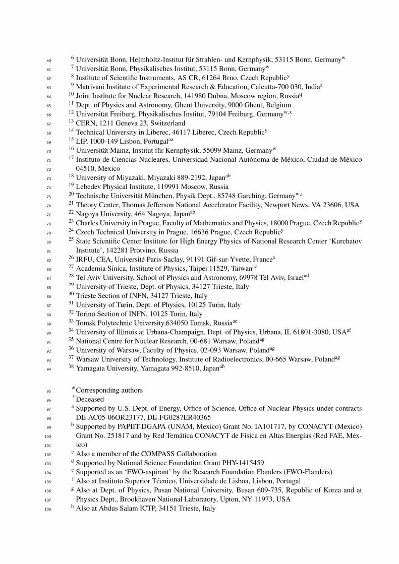
Fig. 3: Amplitude numerator function |∑npj a j Tj(ω(s))| for different values of np. The absolute value is taken as

there is a phase ambiguity because we fit only the intensity ∼ |a(s)|2. Note that each curve is an independent fitfor a specific number of terms np. The curves for np = 4, 5, and 6 all coincide in the resonance region, as shownin the inset.

6

Table 1: Best fit denominator and production parameters for the fit with two CDD poles, sR = 1.5 GeV2, N =

106, c0 = (1.23)2, and the number of expansion parameters np = 6, leading to χ2/d.o.f. = 1.91. Denominatoruncertainties are determined from a bootstrap analysis using 105 random fits. We report no uncertainties on theproduction parameters as they are highly correlated.

Denominator parameters Production parameters [GeV−2]c1 0.532±0.006 GeV−2 a0 0.471c2 0.253±0.007 GeV2 a1 0.134c3 2.38±0.02 GeV2 a2 −1.484g 113±1 GeV4 a3 0.879

a4 2.616a5 −3.652a6 1.821

3 Methodology273

We fit our model to the intensity distribution for π−p→ ηπ−p in the D-wave (56 data points) [2], as274

defined in Eq. (1), by minimizing χ2. We fix the overall scale, N = 106 (see Eq. (1)), and fit the275

coefficients a j (see Eq. (8)), which are then expected to be O(1), and also the parameters in the D(s)276

function. In the first step we obtain the best fit for a given total number of parameters, and in the second277

step we estimate the statistical uncertainties using the bootstrap technique [15, 16, 17, 18, 19]. That278

is to say, we generate 105 pseudodata sets, each data point being resampled according to a Gaussian279

distribution having as mean and standard deviation the original value and error, and we repeat the fit for280

each set. In this way, we obtain 105 different values for the fit parameters, and we take the means and281

standard deviations as expected values and statistical uncertainties, respectively.282

In order to assess the systematic uncertainties we study the dependence of the pole parameters on varia-283

tions of the model, specifically we change i) the number of CDD poles from 1 to 3, ii) the total number284

of terms np in the expansion of the numerator function n(s) in Eq. (8), iii) the value of sR in the left hand285

cut model, iv) the value of teff of the total momentum transfered, and v) the addition of the ρπ channel286

to study coupled-channel effects.287

The fit with CDD∞ only, shown in Fig. 2(a), for sR = 1.5 GeV2 and np = 6 (with a total of 9 parameters),288

captures neither the dip at 1.5 GeV nor the bump at 1.7 GeV. In contrast, the fit with two CDD poles (11289

parameters), shown in Fig. 2(b), captures both features, giving a χ2/d.o.f. = 86.17/(56− 11) = 1.91.290

The parameters corresponding to the best fit with two CDD poles are given in Table 1. The addition of291

another CDD pole does not improve the fit, as the limited precision in the data is incapable of indicating292

any further resonances. Specifically the residue of the additional pole turns out to be compatible with293

zero, leaving the other fit parameters unchanged. We associate no systematic uncertainty to that.294

As discussed earlier, an acceptable numerator function n(s) should be “smooth” in the resonance region,295

i.e. without significant peaks or dips on the scale of the resonance widths. The parameters ci and g of296

the denominator function are related to resonance parameters, while sR controls the distant second sheet297

singularities due to exchange forces. The expansion in n(s), shown in Fig. 3 for sR = 1.5 GeV2 and298

two CDD poles, has a singularity occurring at s =−1.0 GeV2 because of the definition of ω(s) and our299

choice of Λ 3. For variations in n(s) between np = 3 and np = 7, we find the pole positions are relatively300

stable, which we discuss later in our systematic estimates.301

The dependence on teff is expected to affect mostly the overall normalization. Indeed, the variation from302

teff = −1.0 GeV2 to −0.1 GeV2 gives less than 2% difference for the a′2(1700) parameters, and < 1h303

for the a2(1320), and can be neglected compared to the other uncertainties.304

3Note that the production term is not well constrained below s ∼ 1 GeV2, as the phase space and barrier factors highlysuppress the near threshold behavior. The singularity at s =−1 GeV2 however, persist for each np solution.

New analysis of ηπ tensor resonances measured at the COMPASS experiment 7

-10

-5

0

5

10

15

20

0.5 1.0 1.5 2.0 2.5 3.0

Ref(s),

Imf(s)

√s [GeV]

sR = 1.5 GeV2

Re f(s)Im f(s)

Fig. 4: The reduced ηπ → ηπ partial amplitude in the D-wave, f (s) = N(s)/D(s). Shown are the real (red) andimaginary (blue) parts as a function of the ηπ invariant mass with 3σ error band. The node in the imaginary partat 1.7 GeV is due to the total correlation between the real and imaginary parts.

-0.6

-0.5

-0.4

-0.3

-0.2

-0.1

0.0

1.0 1.1 1.2 1.3 1.4 1.5 1.6 1.7 1.8 1.9

−Γ=

2Im

√s p

[GeV

]

m = Re√sp [GeV]

sR = 1.0 GeV2

sR = 1.5 GeV2

sR = 2.0 GeV2

sR = 2.5 GeV2

a2

a′2

-0.120

-0.110

-0.100

1.302 1.306 1.310

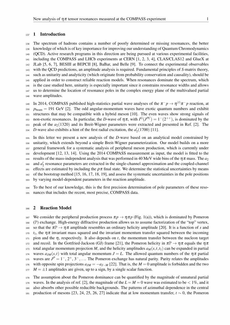
Fig. 5: Location of second-sheet pole positions with two CDD poles, np = 6, and with sR varied from 1.0 GeV2

to 2.5 GeV2. Poles are shown with 2σ (95.5%) confidence level contours from uncertainties computed using 105

bootstrap fits.

4 Results305

This analysis allows us to extract the ηπ → ηπ elastic amplitude in the D-wave. By construction, the306

amplitude has a zero at s = c3. Figure 4 shows the real and imaginary parts of f (s), with the 3σ error307

bands estimated by the bootstrap analysis. Resonance poles are extracted by analytically continuing the308

denominator of the ηπ elastic amplitude to the second Riemann sheet (II) across the unitarity cut using309

DII(s) = D(s)+2iρ(s)N(s). By construction, no first-sheet poles are present. We find three second-sheet310

poles in the energy range of (mπ +mη)≤√

s≤ 3 GeV, two of which can be identified as resonances, as311

shown in Fig. 5 for np = 6 and sR = 1.0,1.5,2.0,2.5 GeV2.312

The mass and width are defined as m = Re√sp and Γ = −2 Im√sp, respectively, where sp is the pole313

position in the s plane. Two of the poles found can be identified as the a2(1320) and a′2(1700) resonances314

in the PDG [11]. The lighter of the two corresponds to the a2(1320). For sR = 1.5 GeV2, the pole has315

mass and width m = (1307±1) MeV and Γ = (112±1) MeV, respectively. The nominal value is the best316

fit pole position, and the uncertainty is the statistical deviation determined from the bootstrap. Values of317

sR between 1.0 and 2.5 GeV2 lead to pole deviations of at most ∆m = 2 MeV and ∆Γ = 3 MeV. The318

heavier pole corresponds to the excited a′2(1700). For sR = 1.5 GeV2, the resonance has mass and width319

8

100

101

102

103

104

105

106

107

0.5 1.0 1.5 2.0 2.5 3.0

Inte

nsity

√s [GeV]

ηπρπ

(a) Coupled CDD parameterization

100

101

102

103

104

105

106

107

0.5 1.0 1.5 2.0 2.5 3.0

Inte

nsity

√s [GeV]

ηπρπ

(b) K-matrix

Fig. 6: Coupled-channel D-wave fit, (a) using a model based on CDD poles, (b) using the standard K-matrixparameterization. Both parameterizations give pole positions consistent with the single-channel analysis. The ηπ

data is taken from Ref. [2] and the ρπ data from Ref. [3].

m = (1720±10) MeV and Γ = (280±10) MeV, respectively. The maximal deviations for the different320

sR values are ∆m = 40 MeV and ∆Γ = 60 MeV. The a2(1320) and a′2(1700) poles (see Fig. 5) are found321

to be stable under variations of sR, which modulates the left hand cut. As expected, there is a third pole322

that depends strongly on sR and reflects the singularity in N(s) modeled as a pole. Its mass ranges from323

1.4 to 3.3 GeV, and its width varies between 1.3 and 1.8 GeV as sR changes from 1 GeV2 to 2.5 GeV2.324

In the limit g→ 0, this pole moves to−sR as expected, while the other two migrate to the real axis above325

threshold [42].326

Changing the number of expansion terms between np = 3 and np = 7 does not in any significant way327

affect the a2(1320) or a′2(1700) pole positions. The maximal deviations are ∆m(a2) = 5 MeV, ∆Γ(a2) =328

7 MeV and ∆m(a′2) = 40 MeV, ∆Γ(a′2) = 30 MeV between three and seven terms in the n(s) expansion.329

In order to demonstrate that coupled-channel effects do not influence the pole positions, we consider an330

extension of the model to include a second channel also measured by COMPASS, ρπ [3], and simulta-331

neously fit the ηπ [2] and the ρπ [3] final states. The branching ratio of the a2(1320) is saturated at the332

level of ∼85% by the ηπ and 3π channels [11], with the ρπ S-wave having the dominant contribution.333

For simplicity we consider the ρ to be a stable particle with mass 775 MeV, the finite width of the ρ being334

relevant only for√

s < 1 GeV. The amplitude is then a j(s) = ∑k [D(s)]−1jk (s) nk(s). The denominator is335

now a 2×2 matrix, whose diagonal elements are of the form given by Eq. (4), with the appropriate phase336

space for each channel. The off-diagonal term is parameterized as a single real constant. The production337

elements nk(s) are as in Eq. (8), with independent coefficients for each channel. We also performed a338

K matrix coupled-channel fit and obtained very similar results that are shown in Figure 6. The coupled-339

channel effects produce a competition between the parameters in the numerators to fit the bump at 1.6340

GeV in ηπ and the dip at 1.8 GeV in ρπ at the same time. The ρπ data prefers not to have any excited341

a′2(1700), which conversely is evident in the ηπ data. Therefore, the uncertainty in the a′2(1700) pole342

position increases, as it is practically unconstrained by the ρπ data. Note, however, that in Ref. [3] the343

dip at√

s∼ 1.8 GeV in the ρπ data is t-dependent, while we use the t-integrated intensity, so it may be344

expected that the effects of the a′2 are suppressed in our combined fit.345

We find the following deviations in the pole positions relative to the single-channel fit: ∆m(a2) = 2 MeV,346

∆Γ(a2) = 3 MeV, ∆m(a′2) = 20 MeV and ∆Γ(a′2) = 10 MeV. These deviations are rather small and we347

quote them within our systematic uncertainties.348

New analysis of ηπ tensor resonances measured at the COMPASS experiment 9

5 Summary and Outlook349

We describe the 2++ wave of π p→ ηπ p reaction in a single-channel analysis emphasizing unitarity and350

analyticity of the amplitude. These fundamental S-matrix principles significantly constrain the possible351

form of the amplitude making the analysis more stable than standard ones that use sums of Breit-Wigner352

resonances with phenomenological background terms.353

The robustness of the model allows us to reliably reproduce the data, and to extract pole positions byanalytical continuation to the complex s-plane. We use the single-energy partial waves in Ref. [2] toextract the pole positions. We find two poles that can be identified as the a2(1320) and the a′2(1700)resonances, with pole parameters

m(a2) = (1307±1±6) MeV, m(a′2) = (1720±10±60) MeV,

Γ(a2) = (112±1±8) MeV, Γ(a′2) = (280±10±70) MeV,

where the first uncertainty is statistical (from the bootstrap analysis) and the second one systematic.354

The systematic uncertainty is obtained adding in quadrature the different systematic effects, i.e. the355

dependence on the number of terms in the expansion of the numerator function n(s), on sR, on teff356

(negligible), and on the coupled-channel effects. The a2 results are consistent with the previous a2(1320)357

results found in Ref. [2]. We note that a new mass-dependent COMPASS analysis of the 3π final state358

using Breit-Wigner forms in 14 waves is in progress.359

The third pole found tends to −sR in the limit of vanishing coupling, indicating that this pole arises from360

the treatment of the exchange forces, and not from the CDD poles that account for the resonances.361

In the future this analysis will be extended to also include the η ′π channel [43], where a large exotic362

P-wave is observed [2].363

Additional material is available online through an interactive website [44, 45].364

Acknowledgments365

We acknowledge the Lilly Endowment, Inc., through its support for the Indiana University Pervasive366

Technology Institute, and the Indiana METACyt Initiative.367

References368

[1] P. Abbon, et al., The COMPASS Setup for Physics with Hadron Beams, Nucl. Instrum. Meth. A779369

(2015) 69–115. arXiv:1410.1797, doi:10.1016/j.nima.2015.01.035.370

[2] C. Adolph, et al., Odd and even partial waves of ηπ− and η ′π− in π−p→ η(′)π−p at 191 GeV/c,371

Phys.Lett. B740 (2015) 303–311. arXiv:1408.4286, doi:10.1016/j.physletb.2014.11.372

058.373

[3] C. Adolph, et al., Resonance Production and ππ S-wave in π−+ p→ π−π−π+ + precoil at 190374

GeV/c, Phys.Rev. D95 (3) (2017) 032004. arXiv:1509.00992, doi:10.1103/PhysRevD.95.375

032004.376

[4] A. A. Alves, Jr., et al., The LHCb Detector at the LHC, JINST 3 (2008) S08005. doi:10.1088/377

1748-0221/3/08/S08005.378

[5] D. I. Glazier, Hadron Spectroscopy with CLAS and CLAS12, Acta Phys.Polon.Supp. 8 (2) (2015)379

503. doi:10.5506/APhysPolBSupp.8.503.380

[6] H. Al Ghoul, et al., First Results from The GlueX Experiment, AIP Conf.Proc. 1735 (2016) 020001.381

arXiv:1512.03699, doi:10.1063/1.4949369.382

[7] H. Al Ghoul, et al., Measurement of the beam asymmetry Σ for π0 and η photoproduction on the383

proton at Eγ = 9 GeVarXiv:1701.08123.384

10

[8] S. Fang, Hadron Spectroscopy at BESIII, Nucl.Part.Phys.Proc. 273-275 (2016) 1949–1954. doi:385

10.1016/j.nuclphysbps.2015.09.315.386

[9] A. J. Bevan, et al., The Physics of the B Factories, Eur.Phys.J. C74 (2014) 3026. arXiv:1406.387

6311, doi:10.1140/epjc/s10052-014-3026-9.388

[10] C. A. Meyer, E. S. Swanson, Hybrid Mesons, Prog.Part.Nucl.Phys. 82 (2015) 21–58. arXiv:389

1502.07276, doi:10.1016/j.ppnp.2015.03.001.390

[11] C. Patrignani, et al., Review of Particle Physics, Chin.Phys. C40 (10) (2016) 100001. doi:10.391

1088/1674-1137/40/10/100001.392

[12] M. Mikhasenko, A. Jackura, B. Ketzer, A. Szczepaniak, Unitarity approach to the mass-dependent393

fit of 3π resonance production data from the COMPASS experiment, EPJ Web Conf. 137 (2017)394

05017. doi:10.1051/epjconf/201713705017.395

[13] A. Jackura, M. Mikhasenko, A. Szczepaniak, Amplitude analysis of resonant production in396

three pions, EPJ Web Conf. 130 (2016) 05008. arXiv:1610.04567, doi:10.1051/epjconf/397

201613005008.398

[14] J. Nys, V. Mathieu, C. Fernndez-Ramrez, A. N. Hiller Blin, A. Jackura, M. Mikhasenko, A. Pilloni,399

A. P. Szczepaniak, G. Fox, J. Ryckebusch, Finite-energy sum rules in eta photoproduction off a400

nucleon, Phys.Rev. D95 (3) (2017) 034014. arXiv:1611.04658, doi:10.1103/PhysRevD.95.401

034014.402

[15] W. H. Press, S. A. Teukolsky, W. T. Vetterling, B. P. Flannery, Numerical Recipes in FORTRAN:403

The Art of Scientific Computing, Cambridge University Press, 1992.404

[16] C. Fernandez-Ramırez, I. V. Danilkin, D. M. Manley, V. Mathieu, A. P. Szczepaniak, Coupled-405

channel model for KN scattering in the resonant region, Phys.Rev. D93 (3) (2016) 034029. arXiv:406

1510.07065, doi:10.1103/PhysRevD.93.034029.407

[17] A. N. Hiller Blin, C. Fernandez-Ramırez, A. Jackura, V. Mathieu, V. I. Mokeev, A. Pilloni, A. P.408

Szczepaniak, Studying the Pc(4450) resonance in J/ψ photoproduction off protons, Phys.Rev.409

D94 (3) (2016) 034002. arXiv:1606.08912, doi:10.1103/PhysRevD.94.034002.410

[18] J. Landay, M. Doring, C. Fernandez-Ramırez, B. Hu, R. Molina, Model Selection for Pion Photo-411

production, Phys.Rev. C95 (1) (2017) 015203. arXiv:1610.07547, doi:10.1103/PhysRevC.412

95.015203.413

[19] A. Pilloni, C. Fernandez-Ramırez, A. Jackura, V. Mathieu, M. Mikhasenko, J. Nys, A. P. Szczepa-414

niak, Amplitude analysis and the nature of the Zc(3900) (2016). arXiv:1612.06490.415

[20] P. Hoyer, T. L. Trueman, Unitarity and Crossing in Reggeon-Particle Amplitudes, Phys.Rev. D10416

(1974) 921. doi:10.1103/PhysRevD.10.921.417

[21] K. Gottfried, J. D. Jackson, On the Connection between production mechanism and decay of reso-418

nances at high-energies, Nuovo Cim. 33 (1964) 309–330. doi:10.1007/BF02750195.419

[22] S. U. Chung, T. L. Trueman, Positivity Conditions on the Spin Density Matrix: A Simple420

Parametrization, Phys.Rev. D11 (1975) 633. doi:10.1103/PhysRevD.11.633.421

[23] A. Kirk, et al., New effects observed in central production by the WA102 experiment at the CERN422

Omega spectrometer, in: 28th International Symposium on Multiparticle Dynamics (ISMD 98)423

Delphi, Greece, September 6-11, 1998, 1998. arXiv:hep-ph/9810221.424

URL http://inspirehep.net/record/477305/files/arXiv:hep-ph_9810221.pdf425

[24] D. Barberis, et al., Experimental evidence for a vector like behavior of Pomeron exchange,426

Phys.Lett. B467 (1999) 165–170. arXiv:hep-ex/9909013, doi:10.1016/S0370-2693(99)427

01186-7.428

[25] D. Barberis, et al., A Study of the centrally produced φφ system in pp interactions at 450 GeV/c,429

Phys.Lett. B432 (1998) 436–442. arXiv:hep-ex/9805018, doi:10.1016/S0370-2693(98)430

00661-3.431

New analysis of ηπ tensor resonances measured at the COMPASS experiment 11

[26] D. Barberis, et al., A Study of pseudoscalar states produced centrally in pp interactions432

at 450 GeV/c, Phys.Lett. B427 (1998) 398–402. arXiv:hep-ex/9803029, doi:10.1016/433

S0370-2693(98)00403-1.434

[27] F. E. Close, A. Kirk, A Glueball - qq filter in central hadron production, Phys.Lett. B397 (1997)435

333–338. arXiv:hep-ph/9701222, doi:10.1016/S0370-2693(97)00222-0.436

[28] F. E. Close, G. A. Schuler, Central production of mesons: Exotic states versus pomeron structure,437

Phys.Lett. B458 (1999) 127–136. arXiv:hep-ph/9902243, doi:10.1016/S0370-2693(99)438

00450-5.439

[29] T. Arens, O. Nachtmann, M. Diehl, P. V. Landshoff, Some tests for the helicity structure of440

the pomeron in ep collisions, Z.Phys. C74 (1997) 651–669. arXiv:hep-ph/9605376, doi:441

10.1007/s002880050430.442

[30] P. Lebiedowicz, O. Nachtmann, A. Szczurek, Exclusive central diffractive production of scalar and443

pseudoscalar mesons tensorial vs. vectorial pomeron, Annals Phys. 344 (2014) 301–339. arXiv:444

1309.3913, doi:10.1016/j.aop.2014.02.021.445

[31] P. Lebiedowicz, O. Nachtmann, A. Szczurek, Central exclusive diffractive production of π+π−446

continuum, scalar and tensor resonances in pp and pp scattering within tensor pomeron approach,447

Phys. Rev. D93 (5) (2016) 054015. arXiv:1601.04537, doi:10.1103/PhysRevD.93.054015.448

[32] C. Bromberg, et al., Study of A2 production in the reaction π−p→ K0K−p at 50 GeV/c, 100449

GeV/c, 175 GeV/c, Phys.Rev. D27 (1983) 1–11. doi:10.1103/PhysRevD.27.1.450

[33] T. Shimada, A. D. Martin, A. C. Irving, Double Regge Exchange Phenomenology, Nucl.Phys. B142451

(1978) 344–364. doi:10.1016/0550-3213(78)90209-2.452

[34] I. V. Danilkin, C. Fernandez-Ramırez, P. Guo, V. Mathieu, D. Schott, M. Shi, A. P. Szczepaniak,453

Dispersive analysis of ω/φ → 3π, πγ∗, Phys.Rev. D91 (9) (2015) 094029. arXiv:1409.7708,454

doi:10.1103/PhysRevD.91.094029.455

[35] V. N. Gribov, Strong interactions of hadrons at high energies: Gribov lectures on Theoretical456

Physics, Cambridge University Press, 2012.457

URL http://cambridge.org/catalogue/catalogue.asp?isbn=9780521856096458

[36] L. Castillejo, R. H. Dalitz, F. J. Dyson, Low’s scattering equation for the charged and neutral scalar459

theories, Phys.Rev. 101 (1956) 453–458. doi:10.1103/PhysRev.101.453.460

[37] S. C. Frautschi, Regge poles and S-matrix theory, Frontiers in physics, W.A. Benjamin, 1963.461

URL https://books.google.com/books?id=2eBEAAAAIAAJ462

[38] J. T. Londergan, J. Nebreda, J. R. Pelaez, A. Szczepaniak, Identification of non-ordinary mesons463

from the dispersive connection between their poles and their Regge trajectories: The f0(500) res-464

onance, Phys.Lett. B729 (2014) 9–14. arXiv:1311.7552, doi:10.1016/j.physletb.2013.465

12.061.466

[39] S. Godfrey, N. Isgur, Mesons in a Relativized Quark Model with Chromodynamics, Phys.Rev. D32467

(1985) 189–231. doi:10.1103/PhysRevD.32.189.468

[40] J. J. Dudek, R. G. Edwards, B. Joo, M. J. Peardon, D. G. Richards, C. E. Thomas, Isoscalar meson469

spectroscopy from lattice QCD, Phys.Rev. D83 (2011) 111502. arXiv:1102.4299, doi:10.470

1103/PhysRevD.83.111502.471

[41] I. J. R. Aitchison, K-matrix formalism for overlapping resonances, Nucl.Phys. A189 (1972) 417–472

423. doi:10.1016/0375-9474(72)90305-3.473

[42] See Supplemental material. Also on http://www.indiana.edu/~jpac/etapi-compass.php .474

[43] JPAC Collaboration, in preparation.475

[44] V. Mathieu, The Joint Physics Analysis Center Website, AIP Conf.Proc. 1735 (2016) 070004.476

arXiv:1601.01751, doi:10.1063/1.4949452.477

[45] JPAC Collaboration, JPAC Website, http://www.indiana.edu/~jpac/.478