European Journal of Operational Research 252 (2016) 322–333

Contents lists available at ScienceDirect

European Journal of Operational Research

journal homepage: www.elsevier.com/locate/ejor

Innovative Applications of O.R.

Large-network travel time distribution estimation for ambulances

Bradford S. Westgate

∗, Dawn B. Woodard , David S. Matteson , Shane G. Henderson

253 Swanson Academic Center, Alma College, 614 W. Superior St., Alma, MI 48801, United States

a r t i c l e i n f o

Article history:

Received 26 August 2014

Accepted 3 January 2016

Available online 11 January 2016

Keywords:

Transportation

Traffic

OR in health services

Travel time estimation

Markov chain Monte Carlo

a b s t r a c t

We propose a regression approach for estimating the distribution of ambulance travel times between

any two locations in a road network. Our method uses ambulance location data that can be sparse in

both time and network coverage, such as Global Positioning System data. Estimates depend on the path

traveled and on explanatory variables such as the time of day and day of week. By modeling at the

trip level, we account for dependence between travel times on individual road segments. Our method is

parsimonious and computationally tractable for large road networks. We apply our method to estimate

ambulance travel time distributions in Toronto, providing improved estimates compared to a recently

published method and a commercial software package. We also demonstrate our method’s impact on

ambulance fleet management decisions, showing substantial differences between our method and the re-

cently published method in the predicted probability that an ambulance arrives within a time threshold.

© 2016 Elsevier B.V. All rights reserved.

t

n

v

u

t

t

d

I

t

o

a

a

h

c

l

W

s

e

fl

l

s

j

1. Introduction

Estimates of ambulance travel times on arbitrary routes in a

road network are used in ambulance dispatch decisions, base loca-

tion algorithms, and real-time redeployment methods ( Brotcorne,

Laporte, & Semet, 2003; Dean, 2008; Goldberg, 2004; Maxwell,

Restrepo, Henderson, & Topaloglu, 2010; Schmid, 2012 ). In many

of these applications it is important to capture the uncertainty

in the travel time, by predicting the entire travel time distribu-

tion rather than just the expected travel time ( Ingolfsson, Budge, &

Erkut, 2008; Zhen, Wang, Hu, & Chang, 2014 ). For instance, taking

into account uncertainty in the travel time of ambulances to the

scene of an emergency can substantially increase the survival rate

of cardiac patients, by improving fleet management decisions and

thus reducing response times ( Erkut, Ingolfsson, & Erdo ̆gan, 2008;

McLay, 2010 ). Also, ambulance fleet performance is measured by

the fraction of emergency calls for which the response time is less

than a specified threshold, and forecasting this performance mea-

sure requires travel time distribution information ( Mason, 2005 ).

Travel time distributions are also used in applications for other ve-

hicle fleets, including calculation of driving directions for private

vehicles using taxi data ( Yuan et al., 2010 ), allocation of railcars

( Topaloglu, 2006 ), and routing and scheduling of courier vehicles

( Potvin, Xu, & Benyahia, 2006 ).

∗ Corresponding author. Tel.: +1 989 463 7264.

E-mail address: westgatebs@alma.edu (B.S. Westgate).

p

G

t

v

http://dx.doi.org/10.1016/j.ejor.2016.01.004

0377-2217/© 2016 Elsevier B.V. All rights reserved.

We propose a regression approach for estimating the distribu-

ion of an ambulance travel time on an arbitrary route in a road

etwork. The prediction depends on the route and on explanatory

ariables such as the time of day and day of week. Our method

ses information from historical trips on the network, specifically

he total travel time and estimated route for each trip. In order

o predict the travel time distribution for a particular route, we

o not require historical trips that take precisely the same route.

nstead, our statistical approach uses information from all the his-

orical trips by learning shared properties like the effects of time

f day and types of road traversed. The model we use is intuitive

nd its parameters are interpretable. Our method is computation-

lly efficient, scaling effectively to large road networks and large

istorical trip databases.

Two features of ambulance travel times motivate our modeling

hoices. First, ambulances traveling at lights-and-sirens speeds are

ess affected by traffic than other vehicles ( Aladdini, 2010; Kolesar,

alker, & Hausner, 1975; Westgate, Woodard, Matteson, & Hender-

on, 2013 ). Therefore, historical ambulance trips are the most rel-

vant source of information for travel times, and real-time traffic

ow information from other vehicles is less useful. Second, ambu-

ance trips are comparatively rare, implying that ambulance data is

parse in time and road network coverage. Roads that are not ma-

or thoroughfares may have only a few ambulance trips on them

er year.

To estimate the route taken in the historical trips, we use

lobal Positioning System (GPS) measurements taken during

ravel. This source of data is called floating car data or automatic

ehicle location data, and is increasingly available for many types

B.S. Westgate et al. / European Journal of Operational Research 252 (2016) 322–333 323

o

v

G

U

i

d

c

f

d

H

a

t

s

d

p

8

i

t

v

e

t

(

C

a

r

s

h

u

d

e

w

t

W

p

s

l

o

&

c

l

t

t

d

t

r

i

Z

a

t

f

a

p

fl

a

t

c

p

f

t

w

t

a

r

e

(

p

c

e

a

t

r

(

e

o

t

l

W

c

m

t

m

a

a

a

t

W

t

d

m

c

t

a

d

A

n

u

t

e

j

T

a

t

t

o

r

s

d

p

2

i

t

p

s

E

t

s

o

t

s

f vehicles, including ambulances, taxis, and personal vehicles,

ia GPS-enabled smartphones or 2-way navigation devices (e.g.

armin or TomTom) ( Hofleitner, Herring, Abbeel, & Bayen, 2012a ).

nlike other sources of travel time data, it does not require

nstrumentation on the roadway, and thus is the only source of

ata available to estimate travel times that has the prospect of

omprehensive network coverage.

Despite the rise in availability of floating car data, there are still

ew methods available to utilize floating car data for travel time

istribution prediction. Hofleitner, Herring, and Bayen (2012b) and

ofleitner et al. (2012a) take a traffic flow perspective, modeling

t the level of the network link (a road segment between two in-

ersections). They use a dynamic Bayesian network for the unob-

erved traffic conditions on links and model the link travel time

istributions conditional on the traffic state. Their method is ap-

lied to a subset of the San Francisco road network with roughly

00 links, predicting travel times using taxi fleet data and validat-

ng with additional data sources.

In previous work, we introduced a Bayesian model for simul-

aneous travel time distribution and path estimation for a set of

ehicle trips ( Westgate et al., 2013 ). Like Hofleitner et al., we mod-

led travel times at the link level. Our method was applied to es-

imate ambulance travel times on a subregion of Toronto.

In an early paper, Erkut, Fenske, Kabanuk, Gardiner, and Davis

2001) estimate ambulance and fire truck speeds in St. Albert, AB,

anada, as part of a study to select new locations for a fire station

nd ambulance base. They use three road classes (freeway, main

oads, and residential roads), and also account for time-of-day and

eason by estimating different speeds for rush hour and non-rush

our and for summer and winter. They estimate average speeds

sing historical data, interviews with drivers, and road tests. They

o not consider the distribution of travel times.

Jenelius and Koutsopoulos (2013) propose a framework for

stimating the distribution of travel times while incorporating

eather, speed limit, and other explanatory factors. They point out

hat previous approaches such as Hofleitner et al. (2012a , 2012b) ;

estgate et al. (2013) assume that the link travel times are inde-

endent within a vehicle trip, perhaps conditional on the traffic

tate. This contrasts with empirical evidence suggesting that the

ink travel times are strongly correlated, even after conditioning

n time of day and other explanatory factors ( Bernard, Hackney,

Axhausen, 2006; Ramezani & Geroliminis, 2012 ). Therefore, they

apture correlation using a moving average specification for the

ink travel times. Their framework is applied to estimate travel

imes for a particular route in Stockholm.

In contrast to these approaches, we model travel times at the

rip level instead of the link level. This naturally incorporates

ependence between link travel times. The ambulance route is

aken into account in the specification of the trip travel time pa-

ameters, such as the median travel time. This trip-level approach

s related to the regression approach of Budge, Ingolfsson, and

erom (2010b) , who model the travel time distribution for an

mbulance trip as a function of shortest-path distance between

he start and end locations. They assume that the log travel time

ollows a t -distribution, where the centering and scale parameters

re either a nonparametric or parametric function of the shortest-

ath distance. These functional forms enable their method to be

exible but still interpretable. Like them we take a regression

pproach, but we also incorporate dependence on the route taken,

ime of day, and other explanatory factors, justifying our modeling

hoices empirically. This captures the fact that locations near

rimary roads can be reached more quickly than other locations,

or example. A downside of modeling at the trip level is that travel

ime predictions cannot be updated to reflect changing conditions

hile a vehicle is enroute. However, this is not a drawback in

he ambulance setting, because travel time estimates are used for

mbulance dispatch decisions and base placement, rather than for

oute selection.

We use our method to predict ambulance travel times for the

ntire road network of Toronto. The size of the road network

68,272 links) is an order of magnitude larger than in previous ap-

lications of travel time distribution estimation based on floating

ar data ( Budge et al., 2010b; Hofleitner et al., 2012a; Hofleitner

t al., 2012b; Jenelius & Koutsopoulos, 2013; Westgate et al., 2013 ),

nd the number of historical vehicle trips (157,283) is also larger

han these previous applications. We compare the prediction accu-

acy of our method to that of Budge et al. (2010b) , Westgate et al.

2013) , and a commercial software package for mean travel time

stimation. We also consider the effect of various simplifications

f our model, and investigate the accuracy of our model when the

ime effect on travel times is artificially inflated.

Finally, we evaluate the effect of using our method for ambu-

ance fleet management, relative to that of Budge et al. (2010b) .

e select a set of representative ambulance posts in Toronto, and

alculate which ambulance post is estimated to be the closest in

edian travel time to each intersection in Toronto. Many intersec-

ions have different estimated closest posts, according to the two

ethods, so the two methods would recommend that a different

mbulance respond to emergencies at these locations, if the closest

mbulance is dispatched. Next, we calculate the probability that

n ambulance is able to respond on time (within a specified time

hreshold) from the closest post to each intersection of the city.

e find substantial differences in these probabilities between the

wo methods. These appear to arise because our method captures

ifferences in speeds between different types of roads, unlike the

ethod of Budge et al.

Commercially available vehicle travel time estimates typically

onsist of estimated expected travel times rather than distribu-

ion estimates, so they cannot be used to calculate the probability

n ambulance arrives within a time threshold, or for ambulance

eployment algorithms where simulated travel times are needed.

lso, these estimates are calculated for standard vehicle speeds,

ot lights-and-sirens ambulance speeds. However, they are still

seful for point estimation performance comparisons, as long as

hey are corrected for bias. Specifically, we investigate travel time

stimates from TomTom, a maker of navigation devices. Bias ad-

ustment does not fully account for the differences between the

omTom context and ours, so our results should not be interpreted

s an evaluation of the quality of TomToms estimates.

The article is organized as follows. In Section 2 , we introduce

he data from Toronto and highlight the exploratory data analysis

hat motivates our modeling choices. In Section 3 , we introduce

ur statistical model and estimation method. In Section 4 , we give

esults and compare to the alternative methods. We draw conclu-

ions in Section 5 . In Appendices Appendix A –Appendix C , we give

etails on data preprocessing, fastest path estimation, and our im-

lementation of the method of Budge et al.

. Toronto EMS data

We use our method for a study of ambulance travel times

n Toronto, Ontario. The goal is to estimate the distribution of

ime required for an ambulance to drive to the scene of a high-

riority emergency, in which case the ambulance uses lights and

irens, and travels at high speed. The data are provided by Toronto

MS (Emergency Medical Services), and include all such ambulance

rips in Toronto during the years 2007 and 2008. We analyzed a

ubset of these data from the Leaside region of Toronto in previ-

us work ( Westgate et al., 2013 ); here we estimate travel times on

he entire Toronto road network, which consists of 68,272 links.

The data associated with each trip include the approximate

tart and end times and locations of the trip, as well as sparse

324 B.S. Westgate et al. / European Journal of Operational Research 252 (2016) 322–333

t

s

S

t

i

d

o

T

s

c

3

3

a

d

a

a

t

l

e

l

m

c

T

c

f

c

f

c

b

t

l

s

p

t

t

t

t

e

t

t

e

t

v

t

t

e

t

r

p

j

t

t

J

t

GPS location and speed readings during the trip. The GPS mea-

surements are stored every 200 meters or 240 seconds, whichever

comes first (typically the distance constraint is satisfied first for

lights-and-sirens trips).

Cleaning and preprocessing the data is a challenge, due to

factors such as human error in recording the start and end

times and locations of the trips, the presence of trips where the

ambulance doubled back on itself, and the presence of GPS mea-

surement error. These challenges and our preprocessing algorithm

are described in Appendix A . After preprocessing we are left with

157,283 ambulance trips, having removed 20,443 trips. The median

shortest-path distance between the start and end locations is 2530

meters.

To apply our method, we first estimate the path traveled

for each ambulance trip, using the GPS data. Many such “map-

matching” methods could be used ( Lou et al., 20 09; Mason, 20 05;

Quddus, Ochieng, & Noland, 2007; Rahmani & Koutsopoulos, 2013 );

we use the one introduced in ( Westgate, 2013 ).

2.1. Exploratory analysis

Here we highlight exploratory analysis of the Toronto EMS

data, after trip preprocessing. Results from this analysis motivate

the modeling assumptions described in Section 3.1 . After prepro-

cessing, each trip consists of a sequence of GPS readings. To assist

exploratory analysis of the travel time distribution between any

two locations, we map the first and last GPS readings of each trip

to the nearest intersections in the network, to use as estimated

start/end locations (this differs from our travel time model, in

which trips are allowed to start and end in the interior of links).

We collect the most common pairs of start/end intersections for

the trips in the dataset; there are 10 start/end pairs with at least

40 trips between them.

Fig. 1 shows normal Quantile–Quantile (Q–Q) plots for the log

travel times between the four most common start/end pairs in the

dataset. The shortest-path distance between the start and end lo-

cations is shown above each Q–Q plot. Also shown on the Q–Q

plots are 95 percent pointwise confidence bands, under the null

hypothesis that the log travel times are normally distributed. Only

6 percent of the observed travel times in the four plots fall outside

the pointwise confidence bands, which suggests that the lognormal

assumption is reasonable (if it is correct then we expect roughly 5

percent of the observations to fall outside of the bands). Although

nearly all of the points outside the confidence bands occur on a

single one of these four plots, this is not surprising because the

points on a Q–Q plot are strongly dependent. Similar Q–Q plots

have been constructed for the next most common start/end pairs,

and they also suggest lognormal travel times.

The lognormal distribution has been observed in practice and

also used as a model for both link and trip travel times repeatedly

in the literature ( Aladdini, 2010; Alanis, Ingolfsson, & Kolfal, 2013;

Kaparias, Bell, & Belzner, 2008; Mazloumi, Currie, & Rose, 2009 ).

We use the lognormal distribution because it is supported by ex-

ploratory data analysis, and also to provide a parsimonious para-

metric model. Due to the sparseness in data, there are typically

few trips between any two locations in the road network. While

Budge et al. found that ambulance travel times were heavier-tailed

than the lognormal (they used log- t distributions), they did not

condition on the start and end locations of the trips. For the

Toronto ambulance data, if one does not condition on the start

and end locations, the travel time distribution also has heavier tails

than the lognormal.

We also wish to investigate the variability in travel times for

each start/end location pair. Fig. 2 shows a scatterplot of the sam-

ple variances of the log trip travel times for the 100 most common

start/end pairs, plotted against the shortest-path distance between

he pair. There is a general decreasing trend in the variance, the

hape of which suggests the exponential decay model described in

ection 3.1 . This is for the log travel times; on the original scale,

he variances increase with distance. One can also construct a sim-

lar scatterplot where each point represents trips of a similar path

istance, not just between specific locations. In this case, we again

bserve a decreasing trend, but with much less noise than in Fig. 2 .

his is consistent with the results seen by Budge et al., who ob-

erved decreasing coefficient of variation of travel times with in-

reasing distance.

. Modeling and estimation

.1. Travel time modeling

Consider a road network with links indexed by j ∈ { 1 , . . . , J} and

set of vehicle trips on that network indexed by i ∈ { 1 , . . . , I} . Let

j indicate the length of link j . Assume that each trip i begins

nd ends at known locations on the road network (not necessarily

t intersections), and that the sequence of links A i = { A i 1 , . . . , A in i }

raversed by trip i is known. Let f ij denote the known fraction of

ink j used by trip i . For interior links in the path A i , this fraction

quals 1; for the first and last links, it captures the fraction of the

ink actually traversed during the trip.

Based on the results of exploratory analysis in Section 2.1 , we

odel the travel time T i for trip i with a lognormal distribution,

onditional on the route traveled. Specifically,

i

∣∣A i , { f i j } j∈ A i , { d j } j∈ A i ∼ LN

(

μ(i ) + log

(

c +

∑

j∈ A i f i j d j u (i, j)

)

, σ 2 (i )

)

(1)

onditionally independent across trips i , where the functional

orms of μ( i ), u ( i , j ), and σ 2 ( i ) are specified appropriately for the

ontext. This model can be rewritten as T i = R i (c +

∑

j∈ A i f i j d j u (i, j))

or a random lognormal multiplicative factor R i ∼ LN (μ(i ) , σ 2 (i ))

apturing the travel time variability and trip-level effects. The

aseline travel time is given by (c +

∑

j∈ A i f i j d j u (i, j)) , where the

erm u ( i , j ) is a unit travel time (inverse of speed) for trip i on

ink j . The product f ij d j is the distance traveled on link j in trip i ,

o the baseline travel time is a sum of individual link travel times

lus an intercept c > 0. One could also include intersection and

urn effects in the specification, although we have not pursued

his extension.

The intercept c captures, for instance, additional time required

o get up to speed at the beginning of the trip and to slow down at

he end. Its inclusion is similar to the model introduced by Kolesar

t al. (1975) and used by Budge et al. (2010b) , in which the travel

imes depend on the square root of the distance for small dis-

ances, and grow linearly with the distance for large distances.

The unit travel time u ( i , j ) for link j in trip i can depend on

xplanatory factors like the road class, speed limit, and whether

he road is one-way. Additionally, it can depend on the type of

ehicle or the driver. Most simply it can be a link effect, giving

he form u ( i , j ) � u j . However, if there are links with very few

rips, as is the case for ambulance data, this approach yields noisy

stimates of the u j parameters. We specify u ( i , j ) to depend on

he road class, taking u ( i , j ) � u � ( j ) where � ( j) ∈ { 1 , . . . , L } is the

oad class of link j (highway, arterial road, etc.). One could also

artition the road network into R geographic regions, and take u ( i ,

) � u � ( j ), r ( j ) for r( j) ∈ { 1 , . . . , R } , to allow downtown arterial roads

o be distinguished from suburban arterial roads, for example.

The parameters μ( i ) and σ 2 ( i ) for the trip effect can depend on

ime, weather, driver, and other explanatory factors (similarly to

enelius & Koutsopoulos, 2013 ). We use the time bin as an explana-

ory factor, setting μ( i ) � μk ( i ) where the week is divided into time

B.S. Westgate et al. / European Journal of Operational Research 252 (2016) 322–333 325

−2 −1 0 1 2

4.8

5.0

5.2

5.4

Trip distance: 1868 m

Normal Quantiles

Log

Trip

Tra

vel T

imes

−2 −1 0 1 2

4.6

4.8

5.0

5.2

5.4

5.6

Trip distance: 1691 m

Normal Quantiles

Log

Trip

Tra

vel T

imes

−2 −1 0 1 2

4.6

4.8

5.0

5.2

Trip distance: 1606 m

Normal Quantiles

Log

Trip

Tra

vel T

imes

−2 −1 0 1 2

4.2

4.6

5.0

5.4

Trip distance: 1180 m

Normal Quantiles

Log

Trip

Tra

vel T

imes

Fig. 1. Normal Quantile–Quantile plots for travel times between the four most common start/end location pairs in the Toronto EMS dataset.

1000 2000 3000 4000

0.05

0.10

0.15

0.20

Trip distance (m)

Sam

ple

varia

nce

of lo

g tr

avel

tim

es

Fig. 2. Sample variances of log travel times for the 100 most common start/end location pairs in the Toronto EMS dataset.

b

s

g

c

p

σ

t

t

T

t

θ

3

e

t

a

ins k ∈ { 0 , 1 , . . . , K} and μ0 � 0 to ensure model identifiability, i.e.

o that each parameter of the model can be uniquely determined

iven sufficient data.

The log scale variance σ 2 ( i ) is modeled via an exponential de-

ay in the total trip distance d i �

∑

j∈ A i f i j d j , as suggested by ex-

loratory data analysis (see Section 2.1, Fig. 1 ). Specifically, we take2 (i ) � Me −λd i + δ, for parameters M > 0, λ > 0, and δ > 0. With

his choice, the variance of the log travel times approaches δ as the

rip distance increases, and equals M + δ for trips of length zero.

he parameter λ controls how quickly the variability decreases

i

owards δ. The unknown parameters in the model are therefore

� (c, u 1 , . . . , u L , μ1 , . . . , μK , M, δ, λ) .

.2. Estimation

We use a Bayesian formulation to estimate the model param-

ters, which allows uncertainty in the parameter estimates to be

aken into account for travel time predictions. The predictions

re based on the posterior distribution of the parameters, which

s proportional to the prior density (specified below) times the

326 B.S. Westgate et al. / European Journal of Operational Research 252 (2016) 322–333

1

0

l

w

1

p

t

l

m

i

2

l

c

s

p

n

t

a

t

e

t

a

t

m

b

4

u

p

m

o

b

r

C

r

w

a

w

r

d

s

1

a

t

a

s

s

o

t

m

t

(

F

t

C

r

s

e

e

l

likelihood function. The likelihood function is equal to the prod-

uct over trips i of the lognormal density of T i (see Eq. (1) ). We

estimate each parameter and relevant function of the parameters

by its posterior mean, and summarize our uncertainty with a

95 percent interval estimate, the endpoints of which are the

0.025 and 0.975 quantiles of the posterior distribution. Com-

putation of the posterior distribution is done via Markov chain

Tierney (1994) .

We have found results to be robust to moderate changes

in the prior distributions for the unknown parameters

(c, u 1 , . . . , u L , μ1 , . . . , μK , M, δ, λ) , due to the large volume of

data. Results are reported for the following prior distributions,

with mutually independent parameters:

u � ∼ LN (ν� , ξ2 u ) , μk ∼ N (0 , ξ 2

μ) ,

� ∈ { 1 , . . . , L } , k ∈ { 1 , . . . , K} c ∼ Unif (0 , ∞ ) ,

√

M ∼ Unif (0 , ∞ ) , √

δ ∼ Unif (0 , ∞ ) , λ ∼ Unif (0 , ∞ ) .

The constant ν� is a prior estimate of the unit travel time on

the log scale, for road class � . For example, there might be ini-

tial speed estimates for each link in class � , or perhaps known

speed limits or recorded GPS speed data. In such cases, ν� can

be set equal to the mean of the log inverse speeds. We use GPS

speed data recorded during ambulance trips to specify a common

ν� for all � . The constant ξ u captures how strongly we believe our

prior estimate ν� of the log unit travel time. We take ξ u to be

large, allowing the information in the data to dominate the poste-

rior estimate of u � . Specifically, we set ξ u so that there is roughly

95 percent prior probability that u � is within a factor of two of

e ν� , which corresponds to ξu = ( log 2) / 2 . Similarly, ξμ captures our

prior uncertainty in the value of μk , and by the same argument we

set ξμ = ( log 2) / 2 . We have no prior information about c , M , and

δ, so we use uniform priors. Although these uniform prior distri-

butions are non-integrable, the posterior distribution is integrable

and valid. The uniform priors are on the square root of δ and M ,

because the square roots of these parameters are on the scale of

the standard deviation of the log travel times, and it is more ap-

propriate to put a uniform prior on a standard deviation than on a

variance ( Gelman, 2006 ).

To estimate the posterior distribution for each parameter, we

use a Metropolis-within-Gibbs Markov chain Monte Carlo method

( Tierney, 1994 ). Specifically, we use Metropolis–Hastings (M–H) to

update each of the unknown parameters in turn, conditional on

the current values of the other unknown parameters. For exam-

ple, to update the parameter u � , we propose a new value u ∗� ∼LN ( log (u � ) , ψ

2 ) . The proposed sample is accepted with the ap-

propriate M–H acceptance probability, which is the minimum of

1 and the following product of the prior, likelihood, and proposal

density ratios:

LN (u

∗� ;ν� , ξ 2

u )

LN (u � ;ν� , ξ 2 u )

LN (u � ; log (u

∗� ) , ψ

2 )

LN (u

∗� ; log (u � ) , ψ

2 ) .

∏ I i =1 LN

(T i ;μk (i ) + log

(c +

∑

j∈ A i f i j d j u

∗� ( j)

), Me −λd i + δ

)∏ I

i =1 LN

(T i ;μk (i ) + log

(c +

∑

j∈ A i f i j d j u � ( j)

), Me −λd i + δ

) .

The variance ψ

2 is a constant that may be tuned to control the av-

erage acceptance probability, which theoretical evidence suggests

should be roughly 23 percent for optimal efficiency ( Roberts &

Rosenthal, 2001 ).

To obtain the results in this article, we ran each Markov chain

for 120,0 0 0 iterations, including a burn-in period of 20,0 0 0 itera-

tions. To assess the Monte Carlo error, we calculated Monte Carlo

standard errors for each of the parameter estimates, using batch

means ( Kelton & Law, 20 0 0 ). Standard errors are quite low, roughly

–2 percent of the parameter estimate for the μk parameters and

.03–0.2 percent for the other parameters.

The computation time for each Markov chain iteration scales

inearly with the number of vehicle trips, for a fixed road net-

ork. Each Markov chain run for these experiments takes roughly

8 hours on a personal computer, without utilizing parallel com-

uting. Since the likelihood is a product over the terms for each

rip, computation time could be decreased by calculating the like-

ihood terms in parallel batches. The Budge et al. nonparametric

ethod ( Budge et al., 2010b ) is estimated using maximum (penal-

zed) likelihood ( Rigby & Stasinopoulos, 2005 ) and takes roughly

0 minutes on a personal computer. In practice, however, ambu-

ance travel time estimates are updated infrequently, so increased

omputation time is not a severe drawback ( Westgate et al., 2013 ).

The reduced versions of our method (see Section 4.1 ) have

maller computation time than the full method. For each set of

arameters, the computation time is approximately linear in the

umber of parameters. For example, the computation time for es-

imating the road class parameters u � is reduced by approximately

factor of 7 for the model with only one road class, compared to

he full model with seven road classes. The computation time for

stimating the time bin parameters for the model with only one

ime bin is eliminated entirely, because the first parameter μ0 is

lways fixed to 0. A model with two time bins has computation

ime for estimating the time bin parameters reduced by approxi-

ately a factor of 3, compared to the full model with four time

ins.

. Results

Here we give the results of ambulance travel time estimation

sing the Toronto data. We compare our proposed method, our

revious method described in Westgate et al. (2013) , the nonpara-

etric method of Budge et al., and the TomTom predictions. For

ur proposed method, we use seven road classes and four time

ins. Class 1 corresponds to highways, Class 2 to major arterial

oads, Classes 3–6 to smaller-sized roads in decreasing order, and

lass 7 to highway on and off-ramps. These road classes are de-

ived from a digital map provided to us by Toronto EMS, although

e have consolidated some of the rarer classes. For example, there

re multiple types of highway ramps in the Toronto EMS map,

hich we have consolidated into one class. Classes 5–6 generally

epresent local roads with little traffic, while Classes 2–4 represent

ifferent sizes of main roads. Time Bin 0, the baseline bin, corre-

ponds to weekday off-peak times (10 a.m. - 3 p.m., 7–10 p.m.), Bin

to rush hour (6–10 a.m., 3–7 p.m.), Bin 2 to weekend daytime (6

.m. - 10 p.m.), and Bin 3 to late night (10 p.m. - 6 a.m.). We chose

hese bins by observing the change in average GPS speed readings

cross the week.

We split the ambulance trips randomly into two equal-sized

ets, using half of the data to train (estimate the parameters of) the

tatistical models, and the other half as test data for all the meth-

ds. Then we reverse the training and test halves. Results from

hese two experiments are similar. Table 1 gives parameter esti-

ates from our method for the first training set.

The road class parameter estimates appear reasonable. The es-

imated unit travel time u 1 = 0 . 0353 seconds per meter for Class 1

highways) corresponds to approximately 102 kilometers per hour.

or Class 7 (highway on/off ramps), u 7 = 0 . 0450 seconds per me-

er corresponds to approximately 80 kilometers per hour, and for

lass 2 (major arterial roads), u 2 = 0 . 0603 seconds per meter cor-

esponds to approximately 60 kilometers per hour. The estimated

peeds decrease for smaller roads, except for Class 6, the small-

st roads. These roads are relatively uncommon, and the interval

stimate is wider for u 6 than for the other parameters, reflecting

arger uncertainty in the value of u .

6

B.S. Westgate et al. / European Journal of Operational Research 252 (2016) 322–333 327

Table 1

Parameter estimates from our model, with 95 percent intervals expressing parameter uncertainty.

Parameter Description Estimate 95 percent posterior interval Speed Estimate

u 1 Highway 0 .0353 seconds per meter [0.0343, 0.0363] 102 kilometers per hour

u 2 Major arterial road 0 .0603 seconds per meter [0.0600, 0.0606] 60 kilometers per hour

u 3 Large road 0 .0653 seconds per meter [0.0648, 0.0659] 55 kilometers per hour

u 4 Medium road 0 .0779 seconds per meter [0.0769, 0.0791] 46 kilometers per hour

u 5 Small road 0 .1018 seconds per meter [0.0997, 0.1038] 35 kilometers per hour

u 6 Smallest road 0 .0712 seconds per meter [0.0646, 0.0781] 51 kilometers per hour

u 7 Highway ramp 0 .0450 seconds per meter [0.0426, 0.0476] 80 kilometers per hour

μ1 Rush hour bin 0 .0268 [0.0215, 0.0323] –

μ2 Weekend daytime bin −0 .0083 [ −0.0139, −0.0026] –

μ3 Late night bin −0 .0097 [ −0.0150, −0.0044] –

c Travel time intercept 25 .08 seconds [24.52, 25.66] -

M Variance parameter 0 .2064 [0.1932, 0.2203] –

δ Variance parameter 0 .0576 [0.0562, 0.0589] –

λ Variance parameter 0 .0 0 097 [0.0 0 091, 0.0 0104] –

s

r

s

l

t

m

s

p

t

o

t

w

m

o

m

4

s

o

w

a

t

t

t

t

i

t

t

t

u

t

t

t

i

u

d

e

w

s

d

t

g

t

2

(

w

d

p

2

f

u

p

m

p

t

b

a

m

t

f

t

m

e

c

d

i

t

f

t

o

D

t

a

o

l

a

a

r

i

a

c

t

(

s

t

t

p

B

The rush hour time bin parameter estimate μ1 = 0 . 0268 corre-

ponds to a travel time increase of about 2.7 percent for rush hour,

elative to weekday off-peak. The estimates of μ2 and μ3 corre-

pond to roughly 1 percent smaller travel times for weekend and

ate night, relative to weekday off-peak. All these values are close

o zero, indicating that lights-and-sirens ambulance speeds are re-

arkably consistent across time bins, in contrast to standard travel

peeds ( Westgate et al., 2013 ).

Our lognormal model implies that about 95 percent of trips are

redicted to fall within two standard deviations of the median on

he log scale, i.e. within factors of e −2 ×SD and e 2 × SD of the median

n the original scale. So the variance estimate δ = 0 . 0576 means

hat for very long trips about 95 percent of the travel times will be

ithin factors of 0.62 and 1.6 of their median travel time. The esti-

ate M = 0 . 2064 implies that for very short trips about 95 percent

f the travel times will be within factors of 0.36 and 2.8 of their

edian travel time.

.1. Travel time prediction comparison

Next we compare the predictive performance for our method,

everal reduced versions of our method, the nonparametric method

f Budge et al. (2010b) , and the TomTom estimates. Recalling that

e use half of the data for training and the other half for testing

nd then reverse, here we evaluate the accuracy of the predicted

ravel time distribution for trips in the test data. For details on the

raining of the Budge et al. method, see Appendix C . For each test

rip we evaluate the quality of a point estimate of the travel time,

he predictive interval estimate, and the distribution estimate us-

ng appropriate statistical measures. For TomTom we only evaluate

he quality of the point estimate since interval and distribution es-

imates are not available. For the method of Budge et al., we use

he median travel time as a point estimate. For our method, we

se the posterior mean of the median travel time as a point es-

imate. The 95 percent predictive interval from those methods is

aken to be the estimated 0.025 and 0.975 quantiles of the travel

ime distribution.

When using our method to predict the travel time for the trips

n the test data, we obtain predictions under two scenarios: (1)

sing the estimated route taken by the vehicle (based on the GPS

ata), or (2) not using this information. Using the estimated route

mulates a situation in which we know the route that the driver

ill take, for instance if the driver were required to take a route

pecified by the dispatcher. Such control over the route could be

esirable since then the route could be optimally selected using

he most recent traffic conditions. However, most ambulance or-

anizations leave the route choice to the driver, without notifying

he dispatcher of their choice. To emulate this situation, in Scenario

we predict the travel time without using the route information

only using the start and end locations of the trip). In this scenario

e obtain an estimated fastest route according to our model (as

escribed in Appendix B ), and base our predictions on this route.

Budge et al. base their travel time predictions on the shortest-

ath distance between the start and end locations ( Budge et al.,

010b ). In the spirit of Scenario 1, since we have estimated routes

or each ambulance trip, it is natural to extend their method to

se the distance of the estimated route, instead of the shortest-

ath distance. Therefore, we obtain predictions from their original

ethod where the training and test sets both use the shortest-

ath distance, and the extended method where the training and

est sets both use the estimated route.

We perform bias correction for each estimation method, since

ias may be present for a variety of reasons. For example, bias

rises in Scenario 2 introduced above because in this scenario our

ethod treats the ambulance paths differently in the training and

est data. For the training trips the estimated route is used, while

or the test trips the fastest route is used, resulting in a tendency

o underestimate travel times. Bias may also be present in each

ethod due to inaccuracies of the assumed model. The TomTom

stimates are severely biased, because they are intended for vehi-

les traveling at standard speeds, not lights-and-sirens speeds. We

o bias correction on the log scale via cross-validation as described

n previous work ( Westgate et al., 2013 ). Bias correction is done on

he log scale to lessen the impact of outlying travel times.

Results are shown in Table 2 . We report point estimation per-

ormance using the root mean squared error (RMSE, in seconds) of

he point estimate compared to the true time, and using the RMSE

f the log predictions compared to the true log time (“RMSE log”).

ue to the inherent variability in travel times, even a perfect dis-

ribution estimate would have RMSE and RMSE log considerably

bove zero. We report the RMSE log because it is less affected by

utlying travel times than the RMSE. Outliers are present for at

east two reasons; first, a small number of trips were not driven

t typical lights-and-sirens speeds, although they were recorded

s high-priority trips. Second, some trips have high error in the

ecorded GPS locations, in which case the estimated path may be

naccurate.

To evaluate the interval estimates, Table 2 shows the percent-

ge of test trips where the observed travel time falls in the 95 per-

ent predictive interval (the coverage, “Cov. percent”), as well as

he geometric mean width of the 95 percent predictive intervals

“Width”). Coverage close to or above 95 percent combined with

mall interval width is desirable, since it indicates that the predic-

ive distribution is narrowly concentrated around the true travel

ime, while reflecting the true variability in travel times.

Table 2 evaluates the quality of the distribution estimates by re-

orting the continuous ranked probability score (CRPS) ( Gneiting,

alabdaoui, & Raftery, 2007 ). This is a “strictly proper” measure of

328 B.S. Westgate et al. / European Journal of Operational Research 252 (2016) 322–333

Table 2

Travel time prediction performance for the Toronto EMS lights-and-sirens data.

Estimation method RMSE (s) RMSE log Cov. percent Width (s) CRPS (s)

Our method, using estimated route 72.3 0.298 94.4 218.9 34.6

Our method, using fastest route 77.7 0.322 93.1 219.7 37.3

Our method, 1 variability parameter 72.5 0.297 94.1 225.9 35.2

Our method, 1 time bin 72.4 0.298 94.4 219.1 34.7

Our method, 1 road class 76.8 0.312 94.3 231.0 36.7

Extended Budge et al. 74.9 0.302 94.6 229.1 35.7

Budge et al. 79.7 0.325 94.8 248.1 38.3

TomTom 82.1 0.347 NA NA NA

f

f

c

t

f

r

r

p

m

t

m

l

4

W

m

p

t

l

n

o

w

m

t

t

r

e

w

d

e

p

i

s

o

t

m

o

s

w

t

t

a

4

t

s

distribution estimation accuracy, meaning that only a perfect dis-

tribution estimate achieves the lowest expected score ( Gneiting &

Raftery, 2007 ). If F is the estimated distribution function and x is

the observed travel time, CRPS (F ; x ) �

∫ ∞

−∞

[ F (y ) − 1 (y ≥ x ) ] 2

dy is

the integrated square of the difference between F and the em-

pirical distribution function based on the single observation x

( Gneiting et al., 2007 ). A lower value corresponds to a better distri-

bution estimate. Even a perfect distribution estimate would yield a

CRPS value well above zero, due to the inherent variability of travel

times. We report the mean CRPS over the test trips ( Gneiting et al.,

2007 ).

In Table 2 , in addition to reporting the accuracy of our method

under Scenarios 1 and 2, and the accuracy of the competing meth-

ods, we report the accuracy of several simplified versions of our

method under Scenario 1. This indicates whether the simplified

models are as effective as our full model and which aspects of our

full model are the most important. We consider the following sim-

plifications: (a) only one time bin, (b) only one road class, and (c)

only one variability parameter instead of the exponential model.

As seen in Table 2 , our method under Scenario 1 (using the

estimated route) outperforms the Budge et al. method by 8–10

percent in RMSE, RMSE log, and CRPS, and outperforms the ex-

tended Budge et al. method by 1.5–3.5 percent in the same metrics.

Our method’s interval estimates have almost identical coverage to

those of Budge et al. but are narrower on average, by 12 percent

compared to the original Budge et al. method and by 4.5 percent

compared to the extended method. Under Scenario 2, our method

outperforms the original Budge et al. method by 2.6 percent in

CRPS and 1–3 percent in RMSE and RMSE log. Our mean predictive

interval width under this scenario is 11 percent narrower than that

of Budge et al., though with slightly lower coverage. These per-

formance differences are most likely due to our model’s inclusion

of different speeds for the different road classes, as well as time

effects.

Our method outperforms the TomTom estimates by 12–14 per-

cent in RMSE and RMSE log under Scenario 1, and by 5–7 percent

in the same metrics under Scenario 2. Scenario 2 is the more natu-

ral comparison, because we do not specify the route traveled when

obtaining the TomTom estimates, instead allowing TomTom to pick

the optimal route. TomTom’s estimates perform respectably, indi-

cating that after bias correction, standard vehicle data do have pre-

dictive power for lights-and-sirens ambulance trips.

Regarding the reduced versions of our approach, the method

with only one time bin performs essentially as well in all met-

rics as the full method. This observation agrees with results from

other studies, which found that travel times of emergency vehi-

cles were not strongly influenced by time-of-day ( Aladdini, 2010;

Kolesar et al., 1975 ). We investigated this observation further by

artificially inflating the travel times during rush hour, and found

that the method with only one time bin still performed almost as

well as the full method (2 percent worse RMSE) when the rush

hour travel times were inflated by 10 percent. The model with only

one variability parameter performs as well in point estimation but

slightly worse in distribution estimation than the full model.

The method with only one road class performs worse than the

ull method and the other reduced methods in all metrics. There-

ore, it is quite important to allow for varying speeds across road

lasses (see previous work Westgate et al., 2013 ). We also inves-

igated methods with two and four road classes (not shown), and

ound that the largest benefit arose from moving from one to two

oad classes (highway and non-highway). Moving from two to four

oad classes and from four to seven road classes gave smaller im-

rovements. The extended Budge et al. method outperforms our

ethod with one road class. Both models rely only on travel dis-

ance; however, the Budge et al. method is more flexible than our

ethod with one road class, because the point estimates on the

og scale are not restricted to a linear function of distance.

.2. Comparison to our previous method

We also wish to compare to our earlier method as described in

estgate et al. (2013) , referred to as Westgate et al. Our previous

ethod is much more computationally intensive than the method

roposed here because it simultaneously estimates the routes of

he historical trips and travel time parameters of each network

ink. Because of this, we cannot apply it to the entire Toronto road

etwork, so we compare our new method to our previous method

n the subregion of Leaside, Toronto. To ensure a fair comparison,

e do not use the route information for the test trips with either

ethod (i.e., we use Scenario 2 from Section 4.1 ).

For application to the subregion we make one minor change to

he model introduced in Section 3.1 . For the prior distribution on

he variance parameter M , we use an exponential distribution with

ate 5, instead of a uniform distribution. Since the dataset has few

xtremely short trips, posterior estimates of M are unstable unless

e use a prior distribution that prefers smaller values. Failure to

o this can lead to unrealistic travel time predictions for the few

xtremely short trips in the dataset.

Results are summarized in Table 3 . We use the same five resam-

lings of training and test sets from the Toronto subregion data as

n Westgate et al. (2013) . The two methods perform roughly the

ame in terms of RMSE log, and our previous method performs

nly slightly better than our new method in RMSE, even though

he new method is much less computationally intensive. Our new

ethod also has much better coverage of interval estimates than

ur previous method. This is because our previous method as-

umed independence between the travel times on different net-

ork links, which is unrealistic, as discussed in Section 1 . Failing

o take into account the association between link travel times leads

o underestimation of the variability in the total route travel time

nd thus overly narrow interval estimates.

.3. Probability of arrival within a time threshold

In this section, we consider the effect of using different travel

ime distribution estimates on ambulance fleet management. We

elect a set of twenty-five representative ambulance post locations

B.S. Westgate et al. / European Journal of Operational Research 252 (2016) 322–333 329

Table 3

Travel time prediction performance of our proposed method and previous method on the

subregion of Leaside, Toronto.

Estimation method RMSE (s) RMSE log Cov. percent Width (s)

Westgate et al. 37.8 0.332 85.8 75.0

Our method, using fastest route 38.1 0.331 91.3 90.3

Fig. 3. Probability of arriving at each intersection in Toronto from the closest ambulance post within 4 minutes, estimated by our method.

i

t

t

t

t

a

l

t

t

t

e

t

p

w

g

a

a

o

a

i

W

a

4

i

s

X

c

s

a

w

m

i

h

m

t

g

a

d

l

d

t

h

a

m

t

c

o

p

a

i

t

h

b

e

i

w

r

n Toronto, by examining the empirical distribution of start loca-

ions of ambulance trips, and choosing commonly-occurring loca-

ions. These ambulance posts are chosen to compare the travel

ime estimates from our method to the Budge et al. method, and

he figures in this section should not be interpreted to represent

ctual ambulance coverage in Toronto.

For each intersection in Toronto, we determine which ambu-

ance post is the closest. For our method, we use the closest post in

erms of smallest estimated median travel time. This corresponds

o Scenario 2 from Section 4.1 . For the Budge et al. method, we use

he closest post in shortest-path distance. Our method and Budge

t al. sometimes differ in these closest posts. Roughly 5 percent of

he intersections in the city are estimated to be closest to different

osts, according to the two methods. Therefore, the two methods

ould recommend different ambulances to respond to an emer-

ency at that intersection, if the policy is to dispatch the closest

mbulance.

Next we calculate the estimated probability an ambulance is

ble to reach each intersection in Toronto within a time thresh-

ld, responding from the closest post, according to our method

nd the method of Budge et al. Visual displays of these probabil-

ties are called probability-of-coverage maps ( Budge et al., 2010b;

estgate et al., 2013 ). In Fig. 3 , we plot the probability that an

mbulance reaches each intersection from the closest post within

minutes, according to our method. Each intersection is shaded

n gray according to this probability, where darker points corre-

pond to higher probability. The post locations are shown as white

s. The probability of arrival is very high for intersections near the

losest post and becomes lower for intersections farther away.

The arrival probabilities from our method do not decrease

olely as a function of travel distance from the closest post, but

lso incorporate road speeds. This becomes clear in Fig. 4 , where

e plot the differences between the arrival probabilities for our

ethod and the Budge et al. method. The black points represent

ntersections where our method gives at least 15 percentage points

igher probability of arrival within 4 minutes than the Budge et al.

ethod does. Thus, there is a substantial predictive difference be-

ween the two distributions for these intersections. The medium

ray points are intersections where the Budge et al. method gives

t least 15 percentage points higher probability than our method

oes. The light gray points are all other intersections. The ambu-

ance post locations are shown as black Xs.

Most of the intersections that are close to an ambulance post

o not differ by 15 percentage points or more according to the

wo methods, because arrival probabilities from both methods are

igh. Similarly, intersections that are far from all ambulance posts

lso differ by less than 15 percentage points. On the other hand,

any of the intersections that are at an intermediate distance to

he closest ambulance post differ in arrival probability by 15 per-

entage points or more. In fact, this is true for roughly 10 percent

f all the intersections in the city. Many of the points where the

robability from our method is at least 15 percentage points higher

re on or near highways, particularly Highway 401, which is visible

n Fig. 4 as a sequence of black points running horizontally across

he middle of the city. The highway road class speed estimate is

igh, so the method predicts better coverage when a highway can

e used. There is another large collection of black points at the left

dge of the figure that are close to Highway 427.

Many of the intersections where the Budge et al. probability

s at least 15 percentage points higher are in residential areas

here there is no direct path following highways or major arterial

oads. For example, there are no major roads traveling from an

330 B.S. Westgate et al. / European Journal of Operational Research 252 (2016) 322–333

Fig. 4. Differences in the estimated probability of arriving within 4 minutes, between our method and that of Budge et al.

t

T

t

o

f

t

i

2

e

fl

e

T

a

t

s

d

A

T

a

b

D

A

p

r

w

t

e

m

e

a

t

s

ambulance post to the collection of gray points near location

( −10 0 0 0, −70 0 0). Similarly, there is no direct route from an

ambulance post to the collection of gray points near location

( −50 0 0, 70 0 0). Though there are major arterial roads in the area,

it would require a detour to use one. There are smaller roads that

take more direct routes from the ambulance posts, but these road

classes have slower speed estimates.

5. Conclusions

We introduced a parametric model for estimating the distribu-

tion of ambulance travel times between any locations in a road

network. The method uses data from historical ambulance trips

that can be sparse in time and network coverage, and is compu-

tationally tractable for large road networks and large datasets of

vehicle trips. The model parameters are interpretable, and include

effects for the roads traveled by the vehicle and trip-level effects

such as time of day. We used a Bayesian formulation and Markov

chain Monte Carlo method to estimate the model parameters.

We tested the method on a large dataset of ambulance trips

from Toronto. Exploratory analysis of the data indicated that the

distribution of ambulance travel times between two fixed loca-

tions is well modeled by a lognormal distribution, with variability

parameter depending on travel distance. These observations influ-

enced our modeling choices. We compared travel time predictions

from our method with predictions from a recently-published

method by Budge et al. (2010b) and commercially available

travel time estimates from TomTom. We found that our method

outperformed the alternative methods in both point estimation

and distribution estimation. We also compared our method with

the method of Westgate et al. (2013) on a subregion of Toronto,

and found that our method performed almost as well in point

estimation and better in interval estimation, while being far more

computationally efficient.

We also investigated several reduced versions of our method,

to determine which features were the most important. The largest

benefit came from the inclusion of parameters for each road class

in the city, compared to a model with only one road class. How-

ever, there was little benefit in performance from adding mul-

iple time bins across the week vs. a single time bin. In the

oronto dataset, the ambulance travel times do not vary substan-

ially across the day and week, even during rush hour. Because

ther cities or datasets may be more variable in time, we per-

ormed an additional set of experiments by artificially inflating

he difference in travel times between time bins. We found that

f the travel times during rush hour were increased by at least

0 percent, then time bin factors provided a substantial benefit to

stimation.

Finally, we investigated operational differences for ambulance

eet management from using our method vs. the method of Budge

t al. After fixing a set of representative ambulance posts in

oronto, we calculated the probability that an ambulance arrives

t each intersection in the city within 4 minutes, responding from

he closest post. We found that for about 10 percent of the inter-

ections in the city, the two methods gave arrival probabilities that

iffered by more than 15 percentage points.

cknowledgments

We thank Christopher Glessner for his work obtaining the Tom-

om estimates. We also thank Toronto EMS, Dave Lyons, TomTom,

nd The Optima Corporation. This research was partially supported

y NSF Grant CMMI-0926814, NSF Grant DMS-1209103, NSF Grant

MS-1455172, and a Xerox PARC faculty research award.

ppendix A. Preprocessing

For each ambulance trip we have the time the ambulance de-

arted for the scene (enroute time), the arrival time, and GPS

eadings for the ambulance between those two times. Ideally, we

ould use the difference between the enroute and arrival times as

he total trip travel time, and use the GPS readings between the

nroute and arrival times to estimate the path traveled via a map-

atching algorithm. However, the enroute and arrival times are

rror-prone. They are manually recorded inside the ambulance by

button push, and sometimes the button is pushed at the wrong

ime. For example, sometimes the button indicating arrival at the

cene is not pushed until after the ambulance departs from the

B.S. Westgate et al. / European Journal of Operational Research 252 (2016) 322–333 331

Fig. 5. A stylized example of the effect of error in recorded enroute and arrived times.

s

m

e

s

e

F

a

(

t

m

m

n

d

i

E

t

t

c

a

t

d

a

c

f

q

t

c

t

b

b

b

c

G

A

u

r

p

o

t

t

G

b

t

l

O

m

t

o

t

A

t

w

u

a

p

m

m

i

m

m

I

t

fi

o

a

t

m

i

p

c

a

0

t

B

t

c

a

d

t

t

d

m

t

cene. The GPS device continues to record data, so there will be

any consecutive readings with speed 0 in between the recorded

nroute and arrival times, while the ambulance is parked at the

cene. A stylized example of this issue is given in Fig. 5 .

Instead of using these error-prone enroute and arrival times, we

stimate the start and end locations and times using the GPS data.

irst, to extract only the GPS readings where the ambulance was

ctually driving to the scene, we isolate the first “traveling block”

defined below) of GPS points, and discard the rest. Then we take

he first and last GPS points of the traveling block as the esti-

ated start and end locations and times of the trip. Due to GPS

easurement error, these locations are not necessarily on the road

etwork, but the map-matching algorithm we use can handle this

iscrepancy ( Westgate, 2013 ).

Our preprocessing method is the following:

1. For each incident in which the ambulance responds at lights-

and-sirens speeds, extract all GPS points with timestamps be-

tween the recorded enroute and arrived times.

2. For each trip, retain the first “traveling block” of GPS points,

discarding the rest.

Traveling block : A maximal consecutive sequence of GPS read-

ngs, with the requirements:

1. Begins and ends with a non-zero GPS speed.

2. Has at least 3 non-zero speed GPS readings.

3. Has no pair of GPS readings (consecutive or otherwise) with:

(a) Timestamps at least 30 seconds apart but with average

speed < 1.8 kilometers per hour, using straight-line distance.

(b) Timestamps at least 2 minutes apart but with average speed

< 7.2 kilometers per hour, using straight-line distance.

(c) Average speed (straight-line) greater than 360 kilometers

per hour.

4. Has straight-line distance of at least 400 meter between the

first and last GPS readings.

5. Has average speed (based on straight-line distance) between

the first and last GPS readings no greater than 216 kilometers

per hour.

ach of these requirements are designed to eliminate a certain

ype of error. Requirement 1 removes zero-speed GPS readings at

he beginning or end of the trip. Requirement 2 ensures that we

an estimate start and end locations for the trip, with at least one

dditional GPS reading for path estimation. Requirement 3 ensures

hat the trip does not have a long stationary period in the mid-

le, as in Fig. 5 . This requirement also removes trips where the

mbulance turned around, and subsequent GPS readings are very

lose to each other. While this is possible behavior, it is unhelpful

or response time estimation to include these trips. Finally, this re-

uirement also removes trips with severe errors in the GPS times-

amp or location. Errors in the GPS data are not common, but oc-

asionally the data contain successive GPS readings with identical

imestamps but different locations, or GPS readings with impossi-

le locations. Requirements 4 and 5 act similarly to Requirement 3,

ut on the entire trip. Requirement 4 removes trips where the am-

ulance turned around and the first and last GPS reading are very

lose to each other. Requirement 5 removes rare trips where the

PS data are shifted by a very large amount from the true location.

ppendix B. Fastest path estimation

Here we describe the fastest path estimation for our method

nder Scenario 2 of Section 4.1 . As noted in Appendix A , the

ecorded start and end times for the ambulance trips are error-

rone, so the first and last GPS readings in the first traveling block

f the trip are used for the start and end times and locations. Since

hese two locations are not necessarily on the road network, to es-

imate the fastest path we first find the two nearest links to these

PS locations, and use the nearest points on these links as possi-

le start/end locations. These links typically correspond to the two

ravel directions of the nearest road. For each of the four start/end

ocation pairs, we calculate the fastest path in median travel time.

f these four possible paths, we use the one with the smallest

edian travel time as the estimated path. This method ensures

hat we obtain a reasonable path for each trip, which can begin

r end in the interior of a link, and is not hampered by choosing

he “wrong direction” of the nearest link.

ppendix C. Implementation of Budge et al.

In this section, we give details of our implementation of

he nonparametric method of Budge et al. (2010b) . For trip i ,

ith travel time T i and shortest-path distance d i , Budge et al.

se the model log (T i ) = log (m (d i )) + c(d i ) εi , where ε i follows

t -distribution with τ degrees of freedom. They introduced a

arametric method and a nonparametric method for estimating

( d i ) and c ( d i ). We chose to implement their nonparametric

ethod, because they proposed the parametric method for ease of

nterpretation, and concluded that results from the nonparametric

ethod were slightly superior to the results from the parametric

ethod, in terms of the Akaike Information Criterion (AIC) ( Budge,

ngolfsson, & Zerom, 2010a ).

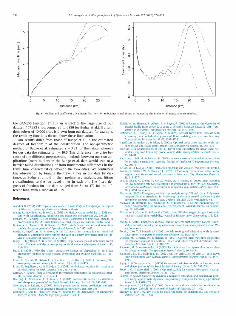
To implement the Budge et al. nonparametric method, we used

he R package GAMLSS ( Stasinopoulos & Rigby, 2007 ). Plots of the

tted median and coefficient of variation functions, for one half

f our dataset (the training data), are given in Fig. 6 . The plots

lso include 95 percent bootstrap confidence bands (pointwise) for

he two functions. Distance is measured in kilometers and time in

inutes, for ease of comparison to the results of Budge et al.

Comparing these plots to Fig. 3 of Budge et al., we observe sim-

lar behavior in the relationship between travel time and shortest-

ath distance. The median travel time function for our data in-

reases between 0 and 10 kilometer, with slightly decreasing slope,

nd the coefficient of variation decreases from 0.5 to slightly above

.2 in that range, as in Budge et al. Our dataset contains some

rips with distance longer than 10 kilometer, while the dataset of

udge et al. does not. However, these trips are rare in our data. Al-

hough our entire dataset is large (157,283 trips), our training data

ontain only 463 trips with distances greater than 10 kilometer

nd 45 trips with distances greater than 15 kilometer. For these

istances, the median travel time function grows more slowly and

hen more quickly, while the coefficient of variation grows and

hen decreases. The confidence bands also widen substantially.

Both the median and coefficient of variation functions for our

ata have non-monotonic fluctuations, though these are much

ore pronounced for the coefficient of variation. These fluctua-

ions remain regardless of the parameters used in implementing

332 B.S. Westgate et al. / European Journal of Operational Research 252 (2016) 322–333

0 5 10 15 20 25

05

1015

20

Distance (km)

Med

ian

trav

el ti

me

(min

.)

0 5 10 15 20 25

0.1

0.2

0.3

0.4

0.5

0.6

Distance (km)

Coe

ffici

ent o

f var

iatio

n

Fig. 6. Median and coefficient of variation functions for ambulance travel times, estimated by the Budge et al. nonparametric method.

H

H

K

K

K

L

M

P

Q

R

R

R

R

S

S

the GAMLSS function. This is an artifact of the large size of our

dataset (157,283 trips, compared to 6886 for Budge et al.). If a ran-

dom subset of 10,0 0 0 trips is drawn from our dataset, for example,

the resulting functions do not show these fluctuations.

Our results differ from those of Budge et al. in the estimated

degrees of freedom τ of the t -distribution. The non-parametric

method of Budge et al. estimated τ = 3 . 71 for their data, whereas

for our data the estimate is τ = 10 . 6 . This difference may arise be-

cause of the different preprocessing methods between our two ap-

plications (more outliers in the Budge et al. data would lead to a

heavier-tailed distribution), or from fundamental differences in the

travel time characteristics between the two cities. We confirmed

this observation by binning the travel times in our data by dis-

tance, as Budge et al. did in their preliminary analysis, and fitting

t -distributions to the log travel times in each bin. The fitted de-

grees of freedom for our data ranged from 5.1 to 172 for the dif-

ferent bins, with a median of 10.9.

References

Aladdini, K. (2010). EMS response time models: A case study and analysis for the region

of Waterloo . University of Waterloo Master’s thesis . Alanis, R. , Ingolfsson, A. , & Kolfal, B. (2013). A Markov chain model for an EMS sys-

tem with repositioning. Production and Operations Management, 22 , 216–231 . Bernard, M. , Hackney, J. , & Axhausen, K. (2006). Correlation of link travel speeds. In

Proceedings of the 6th swiss transport research conference . Ascona, Switzerland . Brotcorne, L. , Laporte, G. , & Semet, F. (2003). Ambulance location and relocation

models. European Journal of Operational Research, 147 , 451–463 .

Budge, S. , Ingolfsson, A. , & Zerom, D. (2010a). Electronic companion to “Empiricalanalysis of ambulance travel times: The case of Calgary emergency medical ser-

vices”. Management Science, 56 , 716–723 . Budge, S. , Ingolfsson, A. , & Zerom, D. (2010b). Empirical analysis of ambulance travel

times: The case of Calgary emergency medical services. Management Science, 56 ,716–723 .

Dean, S. (2008). Why the closest ambulance cannot be dispatched in an urban

emergency medical services system. Prehospital and Disaster Medicine, 23 , 161–165 .

Erkut, E. , Fenske, R. , Kabanuk, S. , Gardiner, Q. , & Davis, J. (2001). Improving theemergency service delivery in St. Albert. Infor, 39 , 416–433 .

Erkut, E. , Ingolfsson, A. , & Erdo ̆gan, G. (2008). Ambulance location for maximumsurvival. Naval Research Logistics (NRL), 55 , 42–58 .

Gelman, A. (2006). Prior distributions for variance parameters in hierarchical mod-els. Bayesian Analysis, 1 , 515–533 .

Gneiting, T. , Balabdaoui, F. , & Raftery, A. (2007). Probabilistic forecasts, calibration

and sharpness. Journal of the Royal Statistical Society: Series B, 69 , 243–268 . Gneiting, T. , & Raftery, A. (2007). Strictly proper scoring rules, prediction, and esti-

mation. Journal of the American Statistical Association, 102 , 359–378 . Goldberg, J. (2004). Operations research models for the deployment of emergency

services vehicles. EMS Management Journal, 1 , 20–39 .

ofleitner, A. , Herring, R. , Abbeel, P. , & Bayen, A. (2012a). Learning the dynamics of

arterial traffic from probe data using a dynamic Bayesian network. IEEE Trans-

actions on Intelligent Transportation Systems, 13 , 1679–1693 . ofleitner, A. , Herring, R. , & Bayen, A. (2012b). Arterial travel time forecast with

streaming data: A hybrid approach of flow modeling and machine learning.Transportation Research Part B, 46 , 1097–1122 .

Ingolfsson, A. , Budge, S. , & Erkut, E. (2008). Optimal ambulance location with ran-dom delays and travel times. Health Care Management Science, 11 , 262–274 .

Jenelius, E. , & Koutsopoulos, H. (2013). Travel time estimation for urban road net-

works using low frequency probe vehicle data. Transportation Research Part B,53 , 64–81 .

aparias, I. , Bell, M. , & Belzner, H. (2008). A new measure of travel time reliabilityfor in-vehicle navigation systems. Journal of Intelligent Transportation Systems,

12 , 202–211 . elton, W. , & Law, A. (20 0 0). Simulation modeling and analysis . McGraw Hill, Boston .

olesar, P. , Walker, W. , & Hausner, J. (1975). Determining the relation between fire

engine travel times and travel distances in New York City. Operations Research,23 , 614–627 .

ou, Y. , Zhang, C. , Zheng, Y. , Xie, X. , Wang, W. , & Huang, Y. (2009). Map-matchingfor low-sampling-rate GPS trajectories. In Proceedings of the 17th ACM SIGSPATIAL

international conference on advances in geographic information systems (pp. 352–361). ACM, New York .

Mason, A. (2005). Emergency vehicle trip analysis using GPS AVL data: A dynamic

program for map matching. In Proceedings of the 40th annual conference of theoperational research society of New Zealand (pp. 295–304). Wellington, NZ .

Maxwell, M. , Restrepo, M. , Henderson, S. , & Topaloglu, H. (2010). Approximate dy-namic programming for ambulance redeployment. INFORMS Journal on Comput-

ing, 22 , 266–281 . azloumi, E. , Currie, G. , & Rose, G. (2009). Using GPS data to gain insight into public

transport travel time variability. Journal of Transportation Engineering, 136 , 623–

631 . McLay, L. (2010). Emergency medical service systems that improve patient surviv-

ability. In Wiley encyclopedia of operations research and management science . Wi-ley, New York .

otvin, J. , Xu, Y. , & Benyahia, I. (2006). Vehicle routing and scheduling with dynamictravel times. Computers & Operations Research, 33 , 1129–1137 .

uddus, M. , Ochieng, W. , & Noland, R. (2007). Current map-matching algorithmsfor transport applications: State-of-the art and future research directions. Trans-

portation Research Part C, 15 , 312–328 .

ahmani, M. , & Koutsopoulos, H. (2013). Path inference from sparse floating car datafor urban networks. Transportation Research Part C, 30 , 41–54 .

amezani, M. , & Geroliminis, N. (2012). On the estimation of arterial route traveltime distribution with Markov chains. Transportation Research Part B, 46 , 1576–

1590 . igby, R. , & Stasinopoulos, D. (2005). Generalized additive models for location, scale

and shape. Journal of the Royal Statistical Society: Series C, 54 , 507–554 .

oberts, G. , & Rosenthal, J. (2001). Optimal scaling for various Metropolis-Hastingsalgorithms. Statistical Science, 16 , 351–367 .

chmid, V. (2012). Solving the dynamic ambulance relocation and dispatching prob-lem using approximate dynamic programming. European Journal of Operational

Research, 219 , 611–621 . tasinopoulos, D. , & Rigby, R. (2007). Generalized additive models for location scale

and shape (GAMLSS) in R. Journal of Statistical Software, 23 , 1–46 .

Tierney, L. (1994). Markov chains for exploring posterior distributions. The Annals ofStatistics, 22 , 1701–1728 .

B.S. Westgate et al. / European Journal of Operational Research 252 (2016) 322–333 333

T

W

W

Y

Z

opaloglu, H. (2006). A parallelizable dynamic fleet management model with ran-dom travel times. European Journal of Operational Research, 175 , 782–805 .

estgate, B. (2013). Vehicle travel time distribution estimation and map-matching viamarkov chain Monte Carlo methods . Cornell University (Ph.D. thesis) .

estgate, B. , Woodard, D. , Matteson, D. , & Henderson, S. (2013). Travel time es-timation for ambulances using Bayesian data augmentation. Annals of Applied

Statistics, 7 , 1139–1161 .

uan, J. , Zheng, Y. , Zhang, C. , Xie, W. , Xie, X. , Sun, G. , & Huang, Y. (2010). T-drive: driving directions based on taxi trajectories. In Proceedings of the 18th

SIGSPATIAL international conference on advances in geographic information systems(pp. 99–108). ACM .

hen, L. , Wang, K. , Hu, H. , & Chang, D. (2014). A simulation optimization frameworkfor ambulance deployment and relocation problems. Computers & Industrial En-

gineering, 72 , 12–23 .