European Journal of Operational Research 263 (2017) 625–638

Contents lists available at ScienceDirect

European Journal of Operational Research

journal homepage: www.elsevier.com/locate/ejor

Innovative Applications of O.R.

Full and fast calibration of the Heston stochastic volatility model

Yiran Cui a , ∗, Sebastian del Baño Rollin

b , Guido Germano

a , c

a Financial Computing and Analytics Group, Department of Computer Science, University College London, Gower Street, London WC1E 6BT, United Kingdom

b School of Mathematical Sciences, Queen Mary University of London, Mile End Road, London E1 4NS, United Kingdom

c Systemic Risk Centre, London School of Economics and Political Science, Houghton Street, London WC2A 2AE, United Kingdom

a r t i c l e i n f o

Article history:

Received 17 May 2016

Accepted 10 May 2017

Available online 17 May 2017

Keywords:

Pricing

Heston model

Model calibration

Optimisation

Levenberg–Marquardt method

a b s t r a c t

This paper presents an algorithm for a complete and efficient calibration of the Heston stochastic volatil-

ity model. We express the calibration as a nonlinear least-squares problem. We exploit a suitable repre-

sentation of the Heston characteristic function and modify it to avoid discontinuities caused by branch

switchings of complex functions. Using this representation, we obtain the analytical gradient of the price

of a vanilla option with respect to the model parameters, which is the key element of all variants of

the objective function. The interdependence between the components of the gradient enables an effi-

cient implementation which is around ten times faster than with a numerical gradient. We choose the

Levenberg–Marquardt method to calibrate the model and do not observe multiple local minima reported

in previous research. Two-dimensional sections show that the objective function is shaped as a narrow

valley with a flat bottom. Our method is the fastest calibration of the Heston model developed so far and

meets the speed requirement of practical trading.

© 2017 Elsevier B.V. All rights reserved.

1

o

a

d

(

p

2

i

t

p

i

p

m

t

c

g

t

a

d

g

t

v

m

t

w

t

m

s

d

d

w

d

w

t

l

b

d

h

0

. Introduction

Pricing financial derivatives is an established problem in the

perational research literature; see for example Fusai, Germano,

nd Marazzina (2016) and references therein contained. Here we

eal with the calibration of the Heston stochastic volatility model

Heston, 1993 ), which is important and popular for derivatives

ricing ( Battauz, De Donno, & Sbuelz, 2014; Beliaeva & Nawalkha,

010; Rouah, 2013 ). The particular topic of model calibration also

nvolves numerical optimisation, which is a core subject of opera-

ional research.

A sophisticated model may reflect the reality better than a sim-

le one, but usually is more challenging to implement and cal-

brate. This is especially true with mathematical models for the

ricing of derivatives and the estimation of risk. The most basic

odel, introduced by Black and Scholes (1973) (BS), assumes that

he underlying price follows a geometric Brownian motion with

onstant drift and volatility. The price of a vanilla option is then

iven as a function of a single parameter, the volatility. However,

he BS model does not adequately take into account essential char-

cteristics of market dynamics such as fat tails and skewness of the

istribution of log returns and the correlation between the value of

∗ Corresponding author.

E-mail addresses: y.cui.12@ucl.ac.uk , cuiyiran2012@hotmail.com

(Y. Cui), s.delbanorollin@qmul.ac.uk (S. del Baño Rollin), g.germano@ucl.ac.uk ,

.germano@lse.ac.uk (G. Germano).

t

c

p

a

ttp://dx.doi.org/10.1016/j.ejor.2017.05.018

377-2217/© 2017 Elsevier B.V. All rights reserved.

he underlying and its volatility. It has also been observed that the

olatility starts to fluctuate when the market reacts to new infor-

ation. Thus, several extensions of the BS model were suggested

hereafter, including the family of stochastic volatility (SV) models,

hich introduces a second Brownian motion to describe the fluc-

uation of the volatility. We study one of the most important SV

odels; it was proposed by Heston (1993) and is defined by the

ystem of stochastic differential equations

S t = μS t d t +

√

v t S t d W

(1) t , (1a)

v t = κ( v − v t )d t + σ√

v t d W

(2) t , (1b)

ith

W

(1) t d W

(2) t = ρd t, (1c)

here S t is the underlying price and v t its variance; the parame-

ers κ, v , σ, ρ are respectively called the mean-reversion rate, the

ong-term variance, the volatility of volatility, and the correlation

etween the Brownian motions W

(1) t and W

(2) t that drive the un-

erlying and its variance; moreover there is a fifth parameter v 0 ,he initial value of the variance.

Model calibration is as crucial as the model itself. Calibration

onsists in determining the parameter values so that the model re-

roduces market prices as accurately as possible. Both the accuracy

nd the speed of calibration are important because practitioners

626 Y. Cui et al. / European Journal of Operational Research 263 (2017) 625–638

2

b

s

2

t

S

t

σ

t

t

s

t

s

w

i

c

e

f

s

w

τt

v

T

m

v

2

a

o

a

i

i

f

t

p

w

m

G

m

w

2

p

l

t

L

M

a

b

e

a

a

I

w

3

d

use the calibrated parameters to price a large number of compli-

cated derivative contracts and to develop high-frequency trading

strategies.

In this paper, we propose to efficiently calibrate the Heston

model using an analytical gradient and numerical optimisation. In

Section 2 , we briefly review the existing research. In Section 3 , we

formulate the objective function and derive its analytical gradient.

In Section 4 , we present a complete algorithm to calibrate the He-

ston model using the Levenberg–Marquardt (LM) method. We also

discuss some points where a carefully designed numerical scheme

may improve the performance. In Section 5 , we present numerical

results.

Throughout, we use bold uppercase letters for matrices, e.g. J ,

and bold lowercase letters for column vectors, e.g. θ; a superscript� for the transpose of a matrix or vector; e for a vector of all ones

[1 , . . . , 1] T ; E[ ·] for expectations; 1 A ( ·) for the indicator function of

the set A ; Re( ·) for the real part and Im( ·) for the imaginary part

of a complex number; ‖·‖ for the l 2 -norm; ‖·‖ ∞

for the l ∞

-norm;

log for the natural logarithm.

2. Previous work on the calibration of the Heston model

In the literature, there are two main approaches to calibrate the

Heston model: historical and implied . The first fits historical time

series of the prices of an option with a fixed strike and matu-

rity, typically by the maximum likelihood method or the efficient

method of moments ( Aït-Sahalia & Kimmel, 2007; Fatone, Mariani,

Recchioni, & Zirilli, 2014; Hurn, Lindsay, & McClelland, 2015 ). The

second fits the volatility surface of an underlying at a fixed time,

i.e., options with several strikes and maturities, to obtain the im-

plied parameter set. Our work follows the second approach, as that

is what is used in real-time pricing and risk management. In the

following, we survey obstacles and existing methods for the Hes-

ton model calibration related to the second approach.

2.1. Recognised difficulties

Firstly, the calibration is in a five-dimensional space. There is

no consensus among researchers on whether the objective func-

tion for the Heston model calibration is convex or irregular. The

results of some proposed methods ( Chen, 2007; Gilli & Schumann,

2012a; Mikhailov & Nögel, 2003 ) depend on the initial point, which

was attributed to a non-convex objective function, but might sim-

ply reflect on the inadequacy of the methods. To find a reasonable

initial guess, short-term or long-term asymptotic rules are used;

see Jacquier and Martini (2011) for a detailed review. However, re-

cently Gerlich, Giese, Maruhn, and Sachs (2012) claimed a conver-

gence to the unique solution independent of the initial guess and

suggested that the Heston calibration problem may have some in-

herent structure leading to a single stationary point. On the other

hand, dependencies among the parameters do exist. For example,

it is known that κ and σ offset each other: lim t→ + ∞

Var (v t ) =σ 2 v /κ, so that a parameter set with large values of κ and σ gives

a fit comparable to a set with small values of κ and σ . Intuitively,

the fact that different parameter combinations yield similar values

of the objective function can be due to the objective function being

flat close to the optimum; see Section 5 in this paper.

Secondly, the analytical gradient for the Heston calibration

problem is hard to find and has not been available so far because it

was believed that the expression of the Heston characteristic func-

tion is overly complicated to provide an insightful analytical gra-

dient: of course, a gradient can be obtained with symbolic algebra

packages, but the resulting expressions are intractable. Instead, nu-

merical gradients obtained by finite difference methods have been

used in gradient-based optimisation methods; however, numerical

gradients have a larger computational cost and a lower accuracy.

.2. Existing methods

We review some heuristics to reduce the dimension of the cali-

ration and then the optimisation methods that have been applied

o far.

.2.1. Heuristics for dimension reduction

Since the Heston parameters are closely related to the shape of

he implied volatility surface ( Clark, 2011; Gatheral, 2006; Gilli &

chumann, 2012a; Janek, Kluge, Weron, & Wystup, 2011 ) ( v 0 con-

rols the position of the volatility smile, ρ the skewness, κ and

the convexity, and κ times the difference between v 0 and vhe term structure of implied volatility), effort s have been made

o simplify the calibration to a lower dimension by presuming

ome of the parameter values based on knowledge available for

he specific volatility surface. The initial variance v 0 is usually

et to the short-term at-the-money (ATM) BS implied variance,

hich is based on the term structure of the BS implied volatil-

ty in the Heston model (Gatheral, 2006, pp. 34–35) . A practical

alibration experiment (Chen, 2007, pp. 29–30) verified the lin-

arity between the initial variance and the BS implied variance

or maturities in the range of 1–2 months. Clark (2011 , Eq. (7.3))

uggested the heuristic assumption κ = 2 . 75 /τ and v = σATM

(τ ) ,

here σ ATM

( τ ) is the ATM implied volatility with time to maturity

. Chen (2007) proposed a fast intraday recalibration by fixing κo the same as yesterday’s and v 0 to the 2-month ATM implied

olatility, which are heuristics actually adopted in the industry.

hese assumptions help with an incomplete calibration, but may

isguide the iterate to a limited domain and thus to a wrong con-

ergence point.

.2.2. Stochastic optimisation methods

Researchers who believed that a descent direction is unavail-

ble have devoted their attention to stochastic optimisation meth-

ds, including Wang–Landau ( Chen, 2007 ), differential evolution

nd particle swarm ( Gilli & Schumann, 2012b ), simulated anneal-

ng ( Moodley, 2009 ), etc. To increase the robustness, a determin-

stic search such as Nelder and Mead using the MATLAB function

minsearch is often combined with these stochastic optimisa-

ion algorithms. Almost all research using stochastic techniques re-

orts issues with performance. GPU technology has been applied

ith simulated annealing to speed up the calibration of the SABR

odel, a member of the family of SV models. Using 2 nVIDIA

eforce GTX470 GPUs it took 421.72 seconds to calibrate 12 instru-

ents achieving a 10 −2 maximum error ( Fernández et al., 2013 ),

hich is still too slow for real-time use.

.2.3. Deterministic optimisation methods

Deterministic optimisation solvers available with commercial

ackages have been proved to be unstable as the performance

argely depends on the quality of the initial guess: this applies to

he Excel built-in solver ( Mikhailov & Nögel, 2003 ) and to the MAT-

AB solver lsqnonlin ( Bauer, 2012; Fusai & Roncoroni, 2008;

oodley, 2009 ). Gerlich, Giese, Maruhn, and Sachs (2012) adopted

Gauss–Newton framework and kept the feasibility of the iterates

y projecting to a cone determined by the constraints. The gradi-

nt of the objective function was calculated by finite differences

nd thus costs a large number of function evaluations.

To sum up, existing calibration algorithms are either based on

d hoc assumptions or not fast or stable enough for practical use.

n this work, we will focus on deterministic optimisation methods

ithout any presumption on the values of the parameters.

. Problem formulation and gradient calculation

The idea of calibrating a volatility model is to minimise the

ifference between the vanilla option price calculated with the

Y. Cui et al. / European Journal of Operational Research 263 (2017) 625–638 627

m

f

w

s

t

s

d

b

3

w

p

r

t

r

i

r

p

mθ

w

S

t

o

j

m

T

a

C

s

c

p

t

w

t

u

a

b

(

t

q

v

p

v

t

a

i

t

i

o

t

t

t

t

a

o

w

v

f

t

o

e

m

t

r

o

m

(

H

o

R

t

3

c

p

τ

C

t

P

P

w

t

a

p

C

T

E

odel and the one observed in the market. In this section, we first

ormulate the calibration problem in a least-squares form. Then,

e present the pricing formula of a vanilla option under the He-

ton model with four algebraically equivalent representations of

he characteristic function, discussing their numerical stability and

uitability for analytical derivation. We calculate the analytical gra-

ient of the objective function which can be used in any gradient-

ased optimisation algorithm.

.1. The inverse problem formulation

Denote by C ∗( K i , τ i ) the market price of a vanilla call option

ith strike K i and time to maturity τi := T i − t, C ( θ; K i , τ i ) the

rice computed via the Heston analytical formula (9) with the pa-

ameter vector θ := [ v 0 , v , ρ, κ, σ ] T . We assemble the r esiduals for

he n options to be calibrated

i ( θ) := C( θ; K i , τi ) − C ∗(K i , τi ) , i = 1 , . . . , n (2)

n the residual vector r ( θ) ∈ R

n , i.e.,

( θ) :=

[r 1 ( θ) , r 2 ( θ) , . . . , r n ( θ)

]ᵀ . (3)

We treat the calibration of the Heston model as an inverse

roblem in the nonlinear least-squares form

in

∈ R m f ( θ) , (4)

here m = 5 indicates the dimension, and

f ( θ) :=

1

2

‖ r ( θ) ‖

2 =

1

2

r T ( θ) r ( θ) . (5)

ince there are many more market observations than parameters

o be found, i.e., n � m , the calibration problem is overdetermined.

Our objective function is the sum of squared price differences

n a set of strikes and maturities. The precise choice of the ob-

ective function is not trivial and, in an accounting sense, ulti-

ately depends on the trade population in an actual trading book.

he choice of strikes and maturities is also not trivial. For ex-

mple, choosing the same strikes (even as a percentage of spot;

hristoffersen, Heston, and Jacobs, 2009 , Table 1) will make these

trikes more out of the money (OTM) for shorter maturities; this

ould lead to miscalibration of the longer-dated smile and to com-

utational underflow for the shorter-ended options. To remedy

his, we adopted the standard approach in foreign exchange (FX)

hich uses strikes defined by given values of BS delta (the sensi-

ivity of the BS option price with respect to the spot price of the

nderlying), namely 10% and 25% delta call and put options as well

s the ATM strike (Clark, 2011, Section 3.3) ; see Section 5 .

With regard to the actual objective function, other possi-

ilities have been considered and can lead to different results

Christoffersen & Jacobs, 2004 ). One such function used in indus-

ry is the sum of squared differences of implied volatilities; this

uantity can be approximated dividing the price difference by BS

ega (the sensitivity of the BS option price with respect to the im-

lied volatility) 1 and is relevant when the price bid/offer spread in

olatility terms is independent of strike (Cont & Tankov, 2003, Sec-

ion 13.2) . This is not always the case, as less liquid OTM options

re quoted with a wider bid/offer spread in volatilities. Calibrat-

ng to implied volatility will cause OTM options, with lower vega,

o weigh more in the objective function, and so the resulting cal-

bration, compared to the one based on price, will privilege OTM

1 BS vega is the quantity relevant for calibration to implied volatilities. There are

ther notions of vega. “Model vega” is the sensitivity of the option price in a par-

icular model with respect to volatility. “Trader vega”, used in hedging positions, is

he result of bumping actual market prices prior to calibration and pricing. In FX,

he market practice is to quote OTM options as risk-reversal and strangle volatili-

ies; sensitivities to these quantities are often called rega and sega. The hope is that

ll these different measures are roughly comparable.

φ

ver ATM options. As our algorithm also approximates vega, future

ork might explore the optimisation problem in terms of implied

olatility. However, since we derive the gradient from the pricing

ormula, here it is most straightforward and consistent to minimise

he pricing error.

Before applying any technique to solve the problem (4) and (5) ,

ne needs to bear in mind that the evaluation of C ( θ; K i , τ i ) is

xpensive for the purpose of calibration; hence, one would like to

inimise the number of computations of Eq. (9) when designing

he algorithm. Moreover, the explicit gradient of C ( θ; K i , τ i ) with

espect to θ is not available in the literature as it is deemed to be

verly complicated. This is indeed true if one starts from the com-

only used expressions for the characteristic function by Heston

1993 , Eq. (17)) or Schoutens, Simons, and Tistaert (2004 , Eq. (17)).

owever, as shown in the next section, a more convenient choice

f the functional form of the characteristic function by del Baño

ollin, Ferreiro-Castilla, and Utzet (2010 , Eq. (6)) eases the deriva-

ion of its analytical gradient.

.2. Pricing formula of a vanilla option and representations of the

haracteristic function

For a spot price S t , an interest rate r and a dividend rate q , the

rice of a vanilla call option with strike K and time to maturity

:= T − t is

( θ; K, τ ) = e −rτ E[(S T − K) 1 { S T ≥K } (S T )] (6a)

= e −rτ(E[ S T 1 { S T ≥K } (S T )] − KE[ 1 { S T ≥K } (S T )]

)(6b)

= S t e −qτ P 1 ( θ; K, τ ) − Ke −rτ P 2 ( θ; K, τ ) . (6c)

In the Heston model, P 1 ( θ; K , τ ) and P 2 ( θ; K , τ ) are solutions

o certain pricing PDEs (Heston, 1993, Eq. (12)) and are given as

1 ( θ; K, τ ) =

1

2

+

1

π

∫ ∞

0

Re

(

e −iu log K

S 0

iu

φ( θ; u − i, τ )

φ( θ;−i, τ )

)

d u, (7)

2 ( θ; K, τ ) =

1

2

+

1

π

∫ ∞

0

Re

(

e −iu log K

S 0

iu

φ( θ; u, τ )

)

d u, (8)

here i is the imaginary unit, φ( θ; u , τ ) is the characteristic func-

ion of the logarithm of the stock price process, φ( θ; −i, τ ) = F /S 0 ,

nd F := S t e (r−q ) τ = is the forward price. Thus, the formula for

ricing a vanilla call option becomes

( θ; K, τ ) =

1

2

(S t e −qτ − Ke −rτ )

+

e −rτ

π

[

S 0

∫ ∞

0

Re

(

e −iu log K

S 0

iu

φ( θ; u − i, τ )

)

d u

−K

∫ ∞

0

Re

(

e −iu log K

S 0

iu

φ( θ; u, τ )

)

d u

]

. (9)

he characteristic function was originally given by Heston (1993 ,

q. (17)) as

( θ; u, τ ) := E

[ exp

(iu log

S t

S 0

)] = exp

{

iu log F

S 0

+

κ v σ 2

[(ξ + d) τ − 2 log

1 − g 1 e dτ

1 − g 1

]+

v 0 σ 2

(ξ + d) 1 − e dτ

1 − g 1 e dτ

},

(10)

628 Y. Cui et al. / European Journal of Operational Research 263 (2017) 625–638

)

w

A

A

A

B

l

p

g

e

w

p

a

m

a

l

m

S

w

l

c

l

where

ξ := κ − σρiu, (11a)

d :=

√

ξ 2 + σ 2 (u

2 + iu ) , (11b)

g 1 :=

ξ + d

ξ − d . (11c)

Kahl and Jäckel (2005) pointed out that when evaluating this

form as a function of u for moderate to long maturities, dis-

continuities appear because of the branch switching of the com-

plex power function G

α(u ) = exp (α log G (u )) with G (u ) := (1 −g 1 e

dτ ) / (1 − g 1 ) and α := κ v /σ 2 , which appears in Eq. (10) as a

multivalued complex logarithm. This depends on the fact that G ( u )

has the shape of a spiral as u increases, and when it repeatedly

crosses the negative real axis, the phase of G ( u ) jumps from −π to

π . Then the phase of G

α( u ) changes from −απ to απ , causing a

discontinuity when α is not a natural number.

Albrecher, Mayer, Schoutens, and Tistaert (2007) found that this

happens when the principal value of the complex square root d

is selected, as most numerical implementations of complex func-

tions do, but can be avoided if the second value is used instead.

Albrecher et al. and Lord and Kahl (2010) proved that this alterna-

tive representation, originally proposed by Schoutens, Simons, and

Tistaert (2004 , Eq. (17)), is continuous and gives numerically stable

prices in the full-dimensional and unrestricted parameter space:

φ( θ; u, τ ) = exp

{

iu log F

S 0

+

κ v σ 2

[(ξ − d) τ − 2 log

1 − g 2 e −dτ

1 − g 2

]+

v 0 σ 2

(ξ − d) 1 − e −dτ

1 − g 2 e −dτ

},

(12

where

g 2 :=

ξ − d

ξ + d =

1

g 1 . (13)

Another equivalent form of the characteristic function was pro-

posed later by del Baño Rollin, Ferreiro-Castilla, and Utzet (2010 ,

Eq. (6)). We correct the expression in that paper by adding the

term −κ v ρτ iu /σ to the exponent, resulting in

φ( θ; u, τ ) = exp

(iu log

F

S 0 − κ v ρτ iu

σ− A

)B

2 κ v / σ 2

, (14)

Fig. 1. Trajectories of γ ( u ) and two equivalent forms of log A 2 ( u ) in the complex plane.

τ = 15 . (For interpretation of the reference to colour in the text, the reader is referred to

here

:=

A 1

A 2

, (15a)

1 := (u

2 + iu ) sinh

dτ

2

, (15b)

2 :=

d

v 0 cosh

dτ

2

+

ξ

v 0 sinh

dτ

2

, (15c)

:=

de κτ/ 2

v 0 A 2

. (15d)

Del Baño Rollin et al. introduced their expression to analyse the

og-spot density, and since then it has not been used for any other

urpose. It was obtained by manipulating the complex moment

enerating function; besides being more compact, it replaces the

xponential functions in the exponent with hyperbolic functions,

hich makes the derivatives easier. Therefore, we will use this ex-

ression to obtain the analytical gradient.

However, the same discontinuity problem pointed out by Kahl

nd Jäckel appears here too. It comes from the factor B 2 κ v /σ 2 , or

ore specifically from A 2 in the denominator of B . Fig. 1 a shows

trajectory of γ ( u ) := ( A 2 ( u )log log | A 2 ( u )|)/| A 2 ( u )|. The double-

ogarithmic scaling of the radius compensates the rapid outward

ovement of the spiralling trajectory of A 2 ( u ) ( Albrecher, Mayer,

choutens, & Tistaert, 20 07; Kahl & Jäckel, 20 05 ). For the curve

e adopt the same hue h ∈ [0, 1) as Kahl and Jäckel (2005) , h :=og 10 (u + 1) mod 1 , which means that segments of slowly varying

olour represent rapid movements of A 2 ( u ) as a function of u .

We thus modify the representation by rearranging log A 2 to

og A 2 = log

(d

v 0 cosh

dτ

2

+

ξ

v 0 sinh

dτ

2

)(16a)

= log d(e dτ/ 2 + e −dτ/ 2 ) + ξ (e dτ/ 2 − e −dτ/ 2 )

2 v 0 (16b)

= log (d + ξ ) e dτ/ 2 + (d − ξ ) e −dτ/ 2

2 v 0 (16c)

= log

[e dτ/ 2

(d + ξ

2 v 0 +

d − ξ

2 v 0 e −dτ

)](16d)

The curves were generated using the parameters in Table 1 with time to maturity

the web version of this article.)

Y. Cui et al. / European Journal of Operational Research 263 (2017) 625–638 629

Table 1

Parameters specification.

Model parameters Market parameters

κ 3.00 S 0 1.00

v 0.10 K 1.10

σ 0.25 r 0.02

ρ −0 . 80 q 0

v 0 0.08

t

i

T

a

l

t

s

(

φ

s

n

o

t

p

R

e

a

3

p

F

c

1

c

Table 2

Properties of the four representations of the Heston characteristic function.

Numerically continuous Easily differentiable

Heston ✗ ✗

Schoutens et al. � ✗

del Baño Rollin et al. ✗ �

Cui et al. � �

n

o

3

t

J

a

r

H

F

c

f

∇

∇

T

p

m

K

t

∇

=

dτ

2

+ log

(d + ξ

2 v 0 +

d − ξ

2 v 0 e −dτ

). (16e)

Fig. 1 b shows the trajectories of the two equivalent formula-

ions of log A 2 . The rearrangement (16e) resolves the discontinu-

ties arising from the logarithm with Eq. (15c) as an argument.

hen we insert Eq. (16e) into log B and denote the final expression

s D :

og B = log d

v 0 +

κτ

2

− log A 2 (17a)

= log d

v 0 +

(κ − d) τ

2

− log

(d + ξ

2 v 0 +

d − ξ

2 v 0 e −dτ

)=: D. (17b)

So we propose a new representation of the characteristic func-

ion which is algebraically equivalent to all the previous expres-

ions and does not show the discontinuities of Eqs. (10) and

14) for large maturities:

( θ; u, τ ) = exp

(iu log

F

S 0 − κ v ρτ iu

σ− A +

2 κ v σ 2

D

). (18)

We have discussed four equivalent representations of the He-

ton characteristic function, three from previous research and one

ewly proposed here by us. We compare them in Fig. 2 : the plot of

ur expression is continuous and overlaps Schoutens et al.’s, while

he other two exhibit discontinuities due to the multivalued com-

lex functions. Moreover our expression, like the one by del Baño

ollin et al. from which it was obtained, has the advantage of being

asily differentiable, as shown in the next section. These properties

re summarised in Table 2 .

.3. Analytical gradient

We use ∇ = ∂ /∂ θ for the gradient operator with respect to the

arameter vector θ and ∇ ∇

� for the Hessian operator. For conve-

ig. 2. Four equivalent representations of the Heston characteristic function. The

urves were generated using the parameters in Table 1 with time to maturity τ =

5 . Eq. (10) jumps at u = 1 , Eq. (14) jumps at u = 2 , while Eqs. (12) and (18) are

ontinuous.

w

h

h

h

h

h

h

(

ience, we omit to write the dependence of the residual vector r

n θ.

.3.1. The basic theorem of the analytical gradient

Let J = ∇ r T ∈ R

m ×n be the Jacobian matrix of the residual vec-

or r with elements

ji =

[∂r i ∂θ j

]=

[∂C( θ; K i , τi )

∂θ j

], (19)

nd H (r i ) := ∇ ∇ T

r i ∈ R

m ×m be the Hessian matrix of each residual

i with elements

jk (r i ) =

[∂ 2 r i

∂ θ j ∂ θk

]. (20)

ollowing the nonlinear least-squares formulation (4) and (5) , one

an easily write the gradient and Hessian of the objective function

as

f = J r , (21a)

∇ T

f = J J T +

n ∑

i =1

r i H (r i ) . (21b)

heorem 1. Assume that an underlying asset S follows the Heston

rocess (1). Let θ := [ v 0 , v , ρ, κ, σ ] T be the parameters in the Heston

odel, C ( θ; K , τ ) be the price of a vanilla call option on S with strike

and time to maturity τ . Then the gradient of C ( θ; K , τ ) with respect

o θ is

C( θ; K, τ ) =

e −rτ

π

[ ∫ ∞

0

Re

(

e −iu log K

S 0

iu

∇ φ( θ; u − i, τ )

)

d u

− K

∫ ∞

0

Re

(

e −iu log K

S 0

iu

∇ φ( θ; u, τ )

)

d u

]

, (22)

here ∇ φ( θ; u, τ ) = φ( θ; u, τ ) h (u ) , h (u ) := [ h 1 (u ) , h 2 (u ) , . . . ,

5 (u )] T with elements

1 (u ) = − A

v 0 , (23a)

2 (u ) =

2 κ

σ 2 D − κρτ iu

σ, (23b)

3 (u ) = − ∂A

∂ρ+

2 κ v σ 2 d

(∂d

∂ρ− d

A 2

∂A 2

∂ρ

)− κ v τ iu

σ, (23c)

4 (u ) =

1

σ iu

∂A

∂ρ+

2 v σ 2

D +

2 κ v σ 2 B

∂B

∂κ− v ρτ iu

σ, (23d)

5 (u ) = − ∂A

∂σ− 4 κ v

σ 3 D +

2 κ v σ 2 d

(∂d

∂σ− d

A 2

∂A 2

∂σ

)+

κ v ρτ iu

σ 2 ;

(23e)

ξ , d , A , A 1 , A 2 , B , D , φ( θ; u , τ ) are defined in Eqs. (11a) , (11b) ,

15) , (17b) and (18) , respectively.

630 Y. Cui et al. / European Journal of Operational Research 263 (2017) 625–638

(

n

(

3

a

w

o

R

r

f

w

i

l

F

t

i

a

F

U

a

v

v

t

w

t

t

i

t

g

f

t

p

Proof. Eq. (22) results from differentiating the vanilla option pric-

ing function (9) under the integral sign; this can be done because

the integrand and its gradient are continuous. Then the problem

reduces to the derivation of the gradient of the characteristic func-

tion φ( θ; u , τ ). Starting from Eq. (14) and following the chain rule,

one can get ∇φ( θ; u , τ ) as discussed below.

Since v 0 and v are only in the exponent and are not involved

with the definition of A or B , we directly obtain

∂φ( θ; u, τ )

∂v 0 = − A

v 0 φ( θ; u, τ ) , (24)

∂φ( θ; u, τ )

∂ v =

2 κ log Bφ( θ; u, τ )

σ 2 . (25)

Next we derive the partial derivative with respect to ρ , since it

provides some terms that can be reused for the rest. We have

∂φ( θ; u, τ )

∂ρ= φ( θ; u, τ )

(−κ v τ iu

σ− ∂A

∂ρ

)+ φ( θ; u, τ )

2 κ v σ 2

1

B

∂B

∂ρ

(26a)

= φ( θ; u, τ )

[−κ v τ iu

σ− ∂A

∂ρ+

2 κ v σ 2 d

(∂d

∂ρ− d

A 2

∂A 2

∂ρ

)](26b)

= φ( θ; u, τ )

[− ∂A

∂ρ+

2 κ v σ 2 d

(∂d

∂ρ− d

A 2

∂A 2

∂ρ

)− κ v τ iu

σ

], (26c)

where

∂d

∂ρ= −ξσ iu

d , (27a)

∂A 2

∂ρ= −σ iu (2 + ξτ )

2 dv 0

(ξ cosh

dτ

2

+ d sinh

dτ

2

), (27b)

∂B

∂ρ=

e κτ/ 2

v 0

(1

A 2

∂d

∂ρ− d

A

2 2

∂A 2

∂ρ

), (27c)

∂A 1

∂ρ= − iu (u

2 + iu ) τξσ

2 d cosh

dτ

2

, (27d)

∂A

∂ρ=

1

A 2

∂A 1

∂ρ− A

A 2

∂A 2

∂ρ. (27e)

By merging and rearranging terms, we find that

∂A

∂κ=

i

σu

∂A

∂ρ, (28a)

∂B

∂κ=

i

σu

∂B

∂ρ+

Bτ

2

, (28b)

which are inserted into

∂φ( θ; u, τ )

∂κ= φ( θ; u, τ )

(− ∂A

∂κ+

2 v σ 2

log B +

2 κ v σ 2 B

∂B

∂κ− v ρτ iu

σ

)(29)

to reach expression (23d) . Similarly, Eq. (23e) can be obtained by

applying the chain rule to Eq. (14) , and the intermediate terms for

∂ φ( θ; u , τ )/ ∂ σ can be written in terms of those for ∂ φ( θ; u , τ )/ ∂ ρ ,

that is

∂d

∂σ=

(ρ

σ− 1

ξ

)∂d

∂ρ+

σu

2

d , (30a)

m

w

∂A 1

∂σ=

(u

2 + iu ) τ

2

∂d

∂σcosh

dτ

2

, (30b)

∂A 2

∂σ=

ρ

σ

∂A 2

∂ρ− 2 + τξ

v 0 τξ iu

∂A 1

∂ρ+

στA 1

2 v 0 , (30c)

∂A

∂σ=

1

A 2

∂A 1

∂σ− A

A 2

∂A 2

∂σ. (30d)

In the end, we replace log B appearing in Eqs. (25) and

29) with D , defined in Eq. (17b) , to ensure the numerical conti-

uity of the implementation. �

Next we discuss the computation of the integrands in Eq.

22) and their convergence.

.3.2. Efficient calculation and convergence of the integrands

All integrands have the form Re (φ( θ; u, τ ) h j (u )(K/S 0 )

−iu / (iu ) )

nd h j ( u ) is a product of elementary functions depending on

hich parameter is under consideration. It has been pointed

ut in the original paper by Heston (1993) that the term

e (φ( θ; u, τ )(K/S 0 )

−iu / (iu ) )

is a smooth function that decays

apidly and presents no difficulties; its product with elementary

unctions decreases fast too. A visual example is shown in Fig. 3 ,

ith parameters given in Table 1 . In our time units, τ = 1 is a trad-

ng year made of 252 days.

Denote as u the value of u for which all integrands are not

arger than 10 −8 . For our testing parameter set, we observe in

igs. 3 and 4 that u decreases when τ increases. This is due to

he fact that the more spread-out a function is, the more localised

ts Fourier transform is (see the uncertainty principle in physics):

s τ increases, the probability density of S T stretches out, while its

ourier transform φ( θ; u , τ ) squeezes. More specifically, if X and

are random variables whose probability density functions are,

part of a constant, Fourier pairs of each other, the product of their

ariances is a constant, i.e., Var( X )Var( U ) ≥ 1. Based on this obser-

ation, one can adjust the truncation according to the maturity of

he option and hence do fewer integrand evaluations for options

ith longer maturities.

In order to obtain the integrands in Eq. (22) , one only needs

o compute φ( θ; u , τ ) and h ( u ). After rearranging and merging

erms, we find that calculating h ( u ) can be boiled down to obtain-

ng the intermediate terms (27), (28) and (30). It is favourable that

he components of h ( u ) share these common terms because so the

radient ∇C ( θ; K , τ ) can be obtained by vectorising the quadrature

or all the integrands as illustrated in Algorithm 3.1 .

Algorithm 3.1: Vectorised integration in the Heston gradient.

1 Specify N grid nodes (u k ) N k =1

and N corresponding weights

(w k ) N k =1

.

2 for k = 1 , 2 , . . . , N do

3 Compute φ( θ; u k , τ ) and h (u k ) .

4 end

5 for j = 1 , 2 , . . . , 5 do

6 Compute ∫ ∞

0 K −iu

iu φ( θ; u, τ ) h j (u )d u ≈ ∑ N

k =1 K −iu k

iu k φ( θ; u k , τ ) h j (u k ) w k .

7 end

Due to the interdependence among the components of h ( u ),

his scheme is faster than computing and integrating each com-

onent h j ( u ) individually. Next, we discuss the choice of the nu-

erical integration method and of the key parameters N , u k and

, but we point out that this vectorised quadrature is compatible

k

Y. Cui et al. / European Journal of Operational Research 263 (2017) 625–638 631

Fig. 3. Convergence of the integrands: Re (φ( θ; u, τ )(K/S 0 )

−iu / (iu ) )

in the Heston pricing formula for C ( θ; K , τ ) (dark blue) and Re (φ( θ; u, τ ) h (u )(K/S 0 )

−iu / (iu ) )

in the

components of its gradient ∂ C / ∂ θ (other colours); h j (u ) , j = 1 , . . . , 5 are respectively relevant for ∂ C / ∂ θ j . The black circle indicates the value u where all integrands are

below 10 −8 . (For interpretation of the references to colour in this figure legend, the reader is referred to the web version of this article.)

Fig. 4. As the time to maturity τ increases, the value u for which all integrands

evaluate to 10 −8 or less decreases.

w

t

τ

s

s

u

3

t

w

S

L

a

r

d

d

ε

w

l

i

d

g

s

a

T

a

m

v

t

g

T

i

t

n

ith any numerical integration method. Also note that the evalua-

ion of φ( θ; u k , τ ) h j ( u k ) is independent of K ; therefore for a given

one can factorise the computation of φ( θ; u k , τ ) h j ( u k ) across

trikes: options on a smile with fixed tenor can share this term,

aving computations. We did not implement this, but it may be

seful in other applications.

.3.3. Integration scheme

The computation of the integrals in the pricing function (9) and

he gradient function (22) dominates the cost of calibration. Thus,

e discuss the proper choice of the numerical integration scheme.

pecifically, we compare the trapezoidal rule (TR) and the Gauss-

egendre rule (GL). The integration error for the pricing formula

nd its gradient is plotted in Fig. 5 a and b. The horizontal axis

eports the number of quadrature nodes N and the vertical axis the

ecadic logarithm of the absolute error of integration. The latter is

efined as

integration := | �(N) − �(N max ) | , (31)

here �( N ) is the value of the integration with N nodes, N is se-

ected equidistantly in the range [10, 100], N max should be ∞ and

s chosen as 10 0 0 in our case. For the plots we use 40 options with

ifferent strikes and maturities. More details on these options are

iven in Section 5 .

The error converges faster for GL than TR and has always a

maller variation when more options are involved. In order to

chieve an average accuracy of 10 −8 , GL requires 40 nodes and

R requires 70. In order for the integrations for all the options to

chieve an accuracy at 10 −8 , GL requires 60 nodes and TR requires

uch more than 100.

Besides a fast convergence of its integration error, GL has an ad-

antageous selection of nodes. GL rescales the domain of integra-

ion to [ −1 , +1] , selects nodes that are symmetric around the ori-

in, and assigns the same weight to each symmetric pair of nodes.

hus, a further reduction in computation can be achieved by mak-

ng use of the common terms of a node and its opposite. Based on

hese benefits, we choose the GL integration scheme with about 60

odes to calibrate the Heston model.

632 Y. Cui et al. / European Journal of Operational Research 263 (2017) 625–638

Fig. 5. Integration error in the Heston model: comparison between TR (full blue line for the mean and dotted purple line for the maximum and minimum) and GL (full red

line for the mean and dotted pink line for the maximum and minimum). (For interpretation of the references to colour in this figure legend, the reader is referred to the

web version of this article.)

Table 3

A comparison between numerical and analytical gradients for n = 40 options.

Computational cost Numerical gradient Analytical gradient

CPU time (arbitrary units) 15.8 1.0

Number of integral evaluations 800 80

4

f

1

s

�

w

t

s

f

m

∇

w

v

N

∇

w

p

f

p

p

o

s

s

s

s

i

2

W

p

m

h

u

a

i

I

o

t

B

e

3.3.4. Comparison with numerical gradient

Previous calibration methods approximate the gradient by a fi-

nite difference scheme. A central difference scheme is the approx-

imation

∇ C( θ; K, τ ) ≈ C( θ + ε; K, τ ) − C( θ − ε; K, τ )

2 ε, (32)

where ε := εe and ε is small. Different values of the increment

ε could be chosen for each component θ j ; for simplicity we have

taken it constant. The size of the difference, ε, has a non-trivial

effect on the approximation. An excessively small value of ε is not

able to reflect the overall function behaviour at the point and may

lead to a wrong moving direction. Moreover the numerical gradient

naturally has an error and one cannot expect to find a solution

with a better accuracy than that of the gradient. In most cases,

the iteration stagnates when the error of the objective function is

roughly the same size as the error of the gradient.

Besides the instability caused by an inappropriate choice of ε, a

numerical gradient has a higher computational cost than an an-

alytical gradient. Recall that the evaluation of one option price

C ( θ; K , τ ) requires the evaluation of two integrals as in Eq. (9) .

Let n be the number of options to be calibrated. At each itera-

tion, one needs to compute 20 n integrals if using the finite dif-

ference scheme while only 2 n integrals if using the analytical form

with the vectorised integration scheme. To give a more intuitive

comparison between the two methods, we perform a preliminary

experiment with ε = 10 −4 and n = 40 using the MATLAB function

quadv with an adaptive Simpson rule for the numerical integra-

tion. In Table 3 , we report the CPU time as an average of 500 runs

and the number of calls of the integral function for each method.

In order to give a relative sense of speed that is independent of the

machine, the CPU time for analytical gradient is scaled to unity,

and that for numerical gradient results about 16 times longer.

Considering the 94% of saving in computational time and the

exempt from deciding ε, we propose to use the analytical Heston

gradient with vectorised quadrature in a gradient-based optimisa-

tion algorithm to calibrate the model.

. Calibration using the Levenberg–Marquardt method

In this section, we present the algorithm for a complete and

ast calibration of the Heston model using the LM method ( Moré,

978 ). The LM method is a typical tool to solve a nonlinear least-

quares problem like Eq. (4) . The search step is given by

θ = ( J J T + μI ) −1 ∇ f, (33)

here I is the identity matrix and μ is a damping factor. By adap-

ively adjusting μ, the method changes between the steepest de-

cent method and the Gauss–Newton method: when the iterate is

ar from the optimum, μ is given a large value so that the Hessian

atrix is dominated by the scaled identity matrix

∇ T

f ≈ μI ; (34)

hen the iterate is close to the optimum, μ is assigned a small

alue so that the Hessian matrix is dominated by the Gauss-

ewton approximation

∇ T

f ≈ J J T

, (35)

hich omits the second term

∑ n i =1 r i H (r i ) in Eq. (21b) . The ap-

roximation (35) is reliable when either r i or H ( r i ) is small. The

ormer happens when the problem is a so-called small residual

roblem and the latter happens when f is nearly linear. The view-

oint is that the model should yield small residuals around the

ptimum because otherwise it is an inappropriate model. The He-

ton model has been known to be able to explain the smile and

kew of the volatility surface. Therefore, we conjecture it to be a

mall residual problem and adopt the approximation of the Hes-

ian in Eq. (35) as converging to the optimum. There are various

mplementations of the LM method, such as MINPACK ( Devernay,

007 ), LEVMAR ( Lourakis, 2004 ), sparseLM ( Lourakis, 2010 ), etc.

e adopt the LEVMAR package which is a robust and stable im-

lementation in C/C++ distributed under GNU. Although its docu-

entation does not report a use in computational finance, LEVMARas been integrated into many open source and commercial prod-

cts in other applications such as astrometric calibration and im-

ge processing. See Algorithm 4.1 .

In lines 1 and 5 of Algorithm 4.1 , the option pricing function

s evaluated. In lines 1 and 8, the gradient function is evaluated.

n line 2, the parameters ω and ν0 are given the default values

f LEVMAR . In line 4, a 5 × 5 linear system is solved; in LEVMARhis is done by an LDLT factorisation with the pivoting strategy of

unch, Kaufman, and Parlett (1976) using the LAPACK ( Anderson

t al., 1999 ) routine.

Y. Cui et al. / European Journal of Operational Research 263 (2017) 625–638 633

Algorithm 4.1: Levenberg–Marquardt algorithm to calibrate

the Heston model.

1 Given the initial guess θ0 , compute ‖ r ( θ0 ) ‖ and J 0 .

2 Choose the initial damping factor μ0 = ω max { diag ( J 0 ) } and

ν0 = 2 .

3 for k = 0 , 1 , 2 , . . . do

4 Solve the normal equations (33) for �θk .

5 Compute θk +1 = θk + �θk and ‖ r ( θk +1 ) ‖ . 6 Compute δL = �θk

ᵀ (μk �θk + J k r ( θk )) and

δF = ‖ r ( θk ) ‖ − ‖ r ( θk +1 ) ‖ . 7 if δL > 0 and δF > 0 then

8 Accept the step: compute J k +1 , μk +1 = μk , νk +1 = νk .

9 else

10 Recalculate the step: set μk = μk νk , νk = 2 νk and

repeat from line 4.

11 end

12 if the stopping criterion (36) is met then

13 Break.

14 end

15 end

f

‖‖

w

(

t

d

c

i

5

c

d

i

H

t

t

T

o

5

r

fi

I

2

1

q

s

�

t

o

C

Table 4

Synthetic implied volatility surface σBS (K, τ ) used for calibration. The implied

volatility σBS matches the BS price to the Heston price, i.e. C BS (σBS ; K, τ ) =

C( θ∗; K, τ ) , with the parameter set θ

∗given in Table 1 . The strikes K are computed

from the BS deltas reported in the header.

τ ( days ) �put BS

= −10% �put BS

= −25% �call BS = 50% �call

BS = 25% �call BS = 10%

30 2.5096 1.4359 0.2808 0.2540 0.2369

60 2.4351 1.3216 0.2847 0.2606 0.2417

90 2.3823 1.2955 0.2878 0.2660 0.2489

120 2.3383 1.2677 0.2904 0.2699 0.2548

150 2.2996 1.2407 0.2925 0.2745 0.2598

180 2.2619 1.2166 0.2943 0.2777 0.2641

252 2.1767 1.1671 0.2975 0.2837 0.2722

360 2.0618 1.1136 0.3007 0.2897 0.2803

Table 5

Reasonable ranges to randomly generate Heston model parame-

ters and the average absolute distance between the initial guess

θ0 and the optimum θ∗ .

Range for model parameters Absolute deviation from θ∗

κ (0.50, 5.00) | κ0 − κ∗| 1.5097

v (0.05, 0.95) | v 0 − v ∗| 0.2889

σ (0.05, 0.95) | σ0 − σ ∗| 0.2875

ρ (−0 . 90 , −0 . 10) | ρ0 − ρ∗| 0.2557

v 0 (0.05, 0.95) | (v 0 ) 0 − v ∗0 | 0.3063

p

t

t

t

u

n

i

s

o

r

o

a

T

2

l

a

p

c

o

2

i

c

h

The stopping criterion for the LM algorithm is when one of the

ollowing is satisfied:

r ( θk ) ‖ ≤ ε 1 , (36a)

J k e ‖ ∞

≤ ε 2 , (36b)

‖ �θk ‖

‖ θk ‖

≤ ε 3 , (36c)

here ε 1 , ε 2 and ε 3 are tolerance levels. The first condition

36a) indicates that the iteration is stopped by a desired value of

he objective function (4) and (5) . The second condition (36b) in-

icates that the iteration is stopped by a small gradient. The third

ondition (36c) indicates that the iteration is stopped by a stagnat-

ng update.

. Numerical results

In this section, we present our experimental results for the

alibration of the Heston model. We first describe our synthetic

ata and then report the performance of our calibration method

n comparison with the fastest previous method. We examine the

essian matrix at an optimal solution, which reveals the reason of

he multiple optima observed in previous research. In the end, we

est on three parameterisations that are typical for certain options.

he result justifies the computational efficiency and robustness of

ur method for practical problems.

.1. Data

To check whether the optimal parameter set found by the algo-

ithm is the global optimum, we used the parameter set θ∗ speci-

ed in Table 1 to generate the implied volatility surface in Table 4 .

ts 40 values are characterised by the call options with �call = 50%,

5% and 10%, and by the put options with �put = −25% and

0%, each with maturities from 30 to 360 days. As we assume

= 0, �call = 50% corresponds to the standard ATM delta-neutral

traddle; moreover, the put-call parity C − P = e −rτ (F − K) impliescall − �put = e −qτ = 1 , i.e. �put = −25% and −10% correspond

o �call = 75% and 90%. Here �call and �put are the BS delta

f a call or put option, i.e. the sensitivity of the BS call price

or the BS put price P with respect to the underlying spot

BS BS

rice S t : to obtain the relevant strikes, one solves for K the equa-

ions �call BS

:= ∂ C BS (K, τ ) /∂ S t = 0 . 50 , 0 . 25 and 0 . 10 , and the equa-

ions �put BS

:= ∂ P BS (K, τ ) /∂ S t = −0 . 10 and − 0 . 25 . The FX conven-

ion of quoting option strikes by their delta has the effect that val-

es close in the strike axis have a comparable likelihood, which is

ot the case with strikes quoted as absolute numbers. The target

s thus to find a parameter set θ† that can replicate the volatility

urface in Table 4 . If θ† is far from θ∗ or, in other words, depends

n the initial guess θ0 , then one concludes that local optimal pa-

ameter sets exist. Otherwise the problem presents only a global

ptimum.

We validated our method using different optimal parameters

nd initial guesses within a reasonable range given in Table 5 .

he procedure is described in Algorithm 5.1 . The Feller condition

Algorithm 5.1: Validation procedure.

1 for i = 1 , 2 , . . . , 100 do

2 Generate a vector of parameters θ∗i , each component of

which is an independent uniformly distributed random

number in the interval specified in Table 5.

3 for j = 1 , 2 , . . . , 100 do

4 Generate an initial guess θ0 j , each component of

which is an independent uniformly distributed random

number in the interval specified in Table 4.

5 Validate Algorithm 4.1 using the initial guess θ0 j to

find θ∗i .

6 end

7 end

κ v /σ 2 > 1 , which ensures that the volatility v (t) is always strictly

arger than zero rather than just non-negative ( 2 κ v /σ 2 is known

s the Feller ratio), was not enforced by us either generating the

arameters and guesses or as a constraint in the LM method be-

ause prices are nevertheless legitimate and the Feller condition is

ften violated in practice ( Albrecher, Mayer, Schoutens, & Tistaert,

007 ), especially in the FX market (Clark, 2011, Table 6.3) . Recently

t has been observed that the Feller condition is probably the most

ounterfactual assumption in finance, and relaxing it is not only

armless from the modelling point of view, but also effective for

634 Y. Cui et al. / European Journal of Operational Research 263 (2017) 625–638

Table 6

Optimisation: average results of 10,0 0 0 test cases.

Absolute deviation from θ∗ Error measure Computational cost

| κ† − κ∗| 1 . 54 × 10 −3 ‖ r 0 ‖ 1 . 39 × 10 −1 CPU time (seconds) 0.29

| v † − v ∗| 2 . 40 × 10 −5 ‖ r †‖ 2 . 94 × 10 −11 LM iterations 12.82

| σ † − σ ∗| 3 . 79 × 10 −3 ‖ J † e ‖ ∞ 1 . 47 × 10 −5 Price evaluations 14.57

| ρ† − ρ∗| 1 . 52 × 10 −2 ‖ �θ†‖ 3 . 21 × 10 −4 Gradient evaluations 12.82

| v † 0

− v ∗0 | 6 . 98 × 10 −6 Linear systems solved 13.57

Table 7

Optimisation of the example specified in Table 1 .

Absolute deviation from θ∗ Error measure Computational cost

| κ† − κ∗| 1 . 09 × 10 −3 ‖ r 0 ‖ 4 . 73 × 10 −2 CPU time (seconds) 0.29

| v † − v ∗| 2 . 18 × 10 −6 ‖ r †‖ 1 . 00 × 10 −12 LM iterations 13

| σ † − σ ∗| 4 . 70 × 10 −5 ‖ J † e ‖ ∞ 1 . 21 × 10 −5 Price evaluations 14

| ρ† − ρ∗| 9 . 89 × 10 −6 ‖ �θ†‖ 2 . 50 × 10 −4 Gradient evaluations 13

| v † 0

− v ∗0 | 1 . 18 × 10 −6 Linear systems solved 13

Fig. 6. Convergence of the LM method.

e

a

a

c

s

c

s

t

s

e

p

a

r

F

t

t

T

n

o

o

a

j

c

w

w

ρ

i

t

e

∂

i

u

i

e

p

a

o

t

t

p

f

derivative pricing, because its violation is a natural consequence of

the misspecification of affine models ( Pacati, Pompa, & Renò, 2017 ).

Following this procedure, we validated Algorithm 4.1 with

10,0 0 0 test cases. An average of the distances between the initial

guesses θ0 and the optima θ∗ is given in Table 5 . The results of the

tests are discussed in the next section.

5.2. Performance

The computations were performed on a MacBook Pro with a

2.6 gigahertz Intel Core i5 processor, 8 gigabytes of RAM and OS

X Yosemite version 10.10.5. The pricing and gradient functions for

the Heston model were coded in C++ using Xcode version 7.3.1. We

used LEVMAR version 2.6 ( Lourakis, 2004 ) as the LM solver set-

ting the tolerances in Eqs. (36) to ε 1 = ε 2 = ε 3 = 10 −10 . However,

in our experiments the LM iteration was always stopped by meet-

ing the condition on the objective function (36a) . We used GL in-

tegration with N = 64 nodes and for simplicity we truncated the

upper limit of the integration in Eq. (22) at u = 200 which in all

cases is enough for pricing and calibrating. The code is provided in

the supplementary material.

The proposed method succeeded in finding the presumed pa-

rameter set in 9843 cases out of 10,0 0 0 without any constraints

on the search space and in 9856 cases restraining the search to the

intervals specified in Table 5 . The average CPU time for the whole

calibration process was less than 0.3 seconds. See Table 6 for de-

tailed information on the whole validation set. In Table 7 and in

the rest of this section we specify the information for a represen-

tative example with the parameters θ∗ specified in Table 1 and the

initial guess θ = [1 . 20 , 0 . 20 , 0 . 30 , −0 . 60 , 0 . 20] T .

0

The convergence of the residual r k and the relative distance of

ach parameter towards the optimum is plotted in Fig. 6 . In Fig. 7 a

nd b, we plot the pricing error on the implied volatility surface

t the initial point θ0 and the optimal point θ† , respectively. As

an be seen, the pricing error decreases from 10 −2 to 10 −7 after 13

teps.

This result contrasts the conclusion of previous research: lo-

al optimal parameters are not intrinsically embedded in the He-

ton calibration problem, but rather caused by an objective func-

ion shaped as a narrow valley with a flat bottom and a premature

topping criterion.

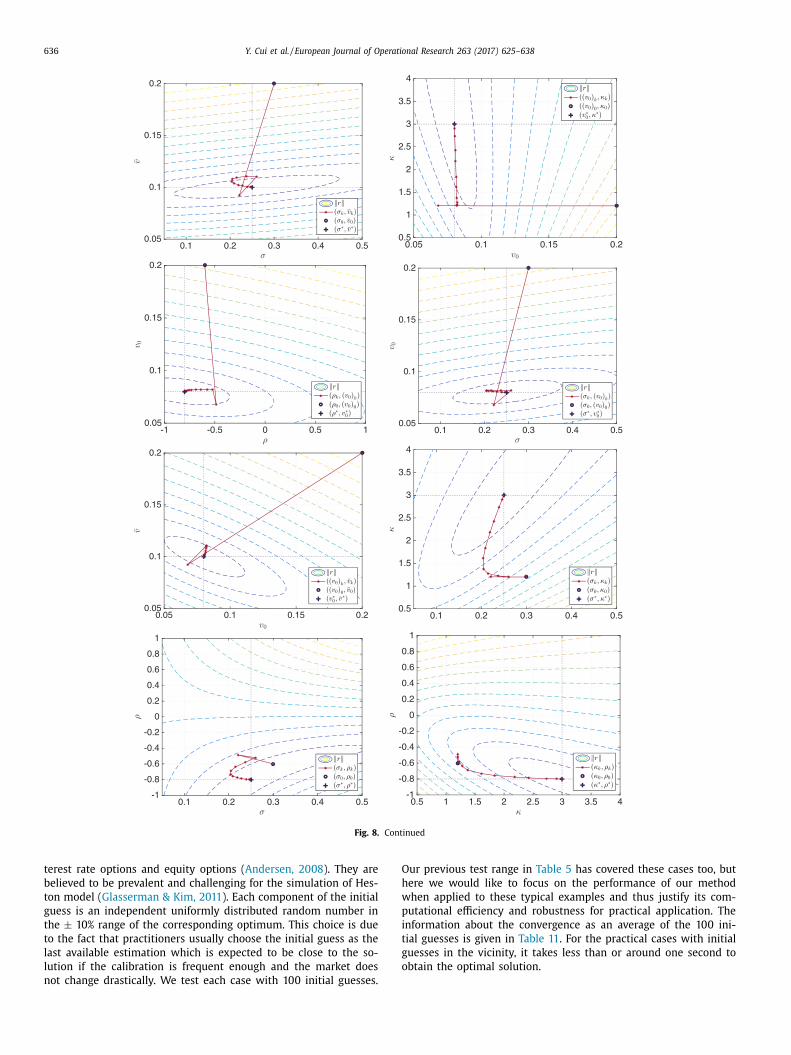
We plot the contours for ‖ r ‖ when varying 2 out of 5 param-

ters. Starting from θ0 , the iteration path is shown with contour

lots in Fig. 8 . The initial point θ0 is marked with a black circle

nd the true solution θ∗ is marked with a black plus symbol. The

ed lines with asterisks are the iteration paths of θk , k = 1 , . . . , 13 .

or almost all pairs, the first step is a long steepest descent step

hat is nearly orthogonal to the contour. The rest are relatively cau-

ious steps with the Gauss–Newton approximation of the Hessian.

he contour plots do not show evidence for local minima, at least

ot in 2-dimensional sections.

The Gauss–Newton approximation of the Hessian matrix at the

ptimal solution is given in Table 8 .

The Hessian matrix is ill-conditioned with a condition number

f 3.98 × 10 6 . The elements ∂ 2 f ( θ∗)/ ∂ κ2 and ∂ 2 f ( θ∗)/ ∂ ρ2 are of

much smaller order than the others. This suggests that the ob-

ective function, when around the optimum, is less sensitive to

hanges of κ and ρ . The effect of κ on the objective function is

eak because option prices depend on the integrated volatility,

hich is little sensitive to the degree of oscillation of volatility;

controls the slope of the smile, so this parameter is difficult to

dentify if a narrow range of moneyness is used for calibration.

In other words, the objective function is more stretched along

hese two axes as can be verified looking at the contours, for

xample in Fig. 8 a and b. The ratio between ∂ 2 f ( θ∗)/ ∂ κ2 and

2 f ( θ∗) /∂ v 2 is of order 10 −6 , which indicates a great disparity

n sensitivity: changing 1 unit of v is comparable to changing 10 6

nits of κ . On the other hand, this explains the so-called local min-

ma reported in previous research. When one starts from a differ-

nt initial point and stops the iteration with a high tolerance, it is

ossible that the iterate lands somewhere in the region where κnd ρ are very different. There are two possible approaches that

ne can seek to deal with this: the first is to scale the parameters

o a similar order and search on a better-scaled objective function;

he second is to decrease the tolerance level for the optimisation

rocess, meaning to approach the very bottom of this objective

unction.

Y. Cui et al. / European Journal of Operational Research 263 (2017) 625–638 635

Fig. 7. Pricing error on the implied volatility surface.

Table 8

Hessian matrix ∇ ∇

�f ( θ∗) at the optimum of the example specified in Table 1 .

∂κ ∂ v ∂σ ∂ρ ∂v 0

∂κ 5 . 26 × 10 −5

∂ v 9 . 65 × 10 −3 2 . 26 × 10 +1

∂σ −5 . 49 × 10 −4 −7 . 66 × 10 −2 7 . 46 × 10 −3

∂ρ 1 . 61 × 10 −4 2 . 00 × 10 −2 −2 . 34 × 10 −3 7 . 56 × 10 −4

∂v 0 5 . 28 × 10 −3 1 . 18 × 10 +1 −3 . 53 × 10 −2 8 . 40 × 10 −3 9 . 69 × 10 −1

Table 9

Performance comparison between solvers.

LMA LMN FPSQP

Stopping criterion ‖ r ( θk ) ‖ ≤ 10 −10 ‖ r ( θk ) ‖ ≤ 10 −10 ‖ �θk ‖ ≤ 10 −6

Iterations 13 22 –

Price evaluations per iteration 1.08 n 1.70 n 6.00 n

a

e

g

a

S

c

u

m

q

m

l

b

a

g

Table 10

Test cases with realistic Heston model

parameters. Case I: long-dated FX op-

tions. Case II: long-dated interest rate

options. Case III: equity options.

Case I Case II Case III

κ∗ 0.50 0.30 1.00

v ∗ 0.04 0.04 0.09

σ ∗ 1.00 0.90 1.00

ρ∗ −0.90 −0.50 −0.30

v ∗0 0.04 0.04 0.09

t

In Table 9 , we present the performance of the LM method with

nalytical gradient (LMA), the LM method with numerical gradi-

nt (LMN), and a feasibility perturbed sequential quadratic pro-

ramming method (FPSQP) ( Gerlich, Giese, Maruhn, & Sachs, 2012 )

dopted in UniCredit bank. As the concrete implementation of FP-

QP is owned by the bank, we only extract their test results. The

omputational cost can be compared through the number of eval-

ations of the pricing function (9) per iteration, expressed as a

ultiple of the number n of options to be calibrated. LMA re-

uires about n pricing function evaluations per step. LMN requires

ore for the gradient approximation, but the difference is not

arge since LMN uses a rank-one update for the subsequent Jaco-

ian matrices. FPSQP requires about 5.5 times more than LMA and

chieves only a lower accuracy for the stopping criterion for the

radient.

r

Fig. 8. Contours of ‖ r ‖ and it

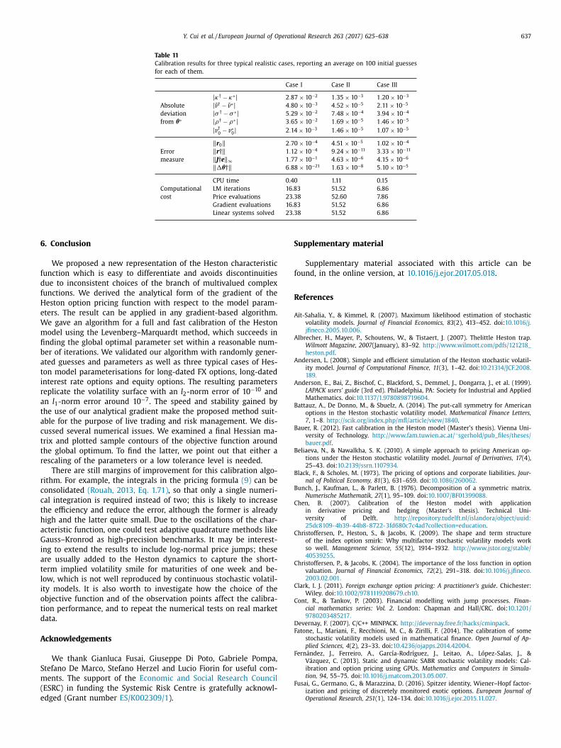
We tested our method also on a few realistic model parame-

erisations. In Table 10 , we present three test cases that are rep-

esentative respectively for long-dated FX options, long-dated in-

eration path for ( θ i , θ j ).

636 Y. Cui et al. / European Journal of Operational Research 263 (2017) 625–638

Fig. 8. Continued

O

h

w

p

i

t

g

o

terest rate options and equity options ( Andersen, 2008 ). They are

believed to be prevalent and challenging for the simulation of Hes-

ton model ( Glasserman & Kim, 2011 ). Each component of the initial

guess is an independent uniformly distributed random number in

the ± 10% range of the corresponding optimum. This choice is due

to the fact that practitioners usually choose the initial guess as the

last available estimation which is expected to be close to the so-

lution if the calibration is frequent enough and the market does

not change drastically. We test each case with 100 initial guesses.

ur previous test range in Table 5 has covered these cases too, but

ere we would like to focus on the performance of our method

hen applied to these typical examples and thus justify its com-

utational efficiency and robustness for practical application. The

nformation about the convergence as an average of the 100 ini-

ial guesses is given in Table 11 . For the practical cases with initial

uesses in the vicinity, it takes less than or around one second to

btain the optimal solution.

Y. Cui et al. / European Journal of Operational Research 263 (2017) 625–638 637

Table 11

Calibration results for three typical realistic cases, reporting an average on 100 initial guesses

for each of them.

Case I Case II Case III

| κ† − κ∗| 2 . 87 × 10 −2 1 . 35 × 10 −3 1 . 20 × 10 −3

Absolute | v † − v ∗| 4 . 80 × 10 −3 4 . 52 × 10 −5 2 . 11 × 10 −5

deviation | σ † − σ ∗| 5 . 29 × 10 −2 7 . 48 × 10 −4 3 . 94 × 10 −4

from θ∗ | ρ† − ρ∗| 3 . 65 × 10 −2 1 . 69 × 10 −5 1 . 46 × 10 −5

| v † 0

− v ∗0 | 2 . 14 × 10 −3 1 . 46 × 10 −5 1 . 07 × 10 −5

‖ r 0 ‖ 2 . 70 × 10 −4 4 . 51 × 10 −5 1 . 02 × 10 −4

Error ‖ r †‖ 1 . 12 × 10 −4 9 . 24 × 10 −11 3 . 33 × 10 −11

measure ‖ J † e ‖ ∞ 1 . 77 × 10 −1 4 . 63 × 10 −6 4 . 15 × 10 −6

‖ �θ†‖ 6 . 88 × 10 −21 1 . 63 × 10 −8 5 . 10 × 10 −5

CPU time 0.40 1.11 0.15

Computational LM iterations 16.83 51.52 6.86

cost Price evaluations 23.38 52.60 7.86

Gradient evaluations 16.83 51.52 6.86

Linear systems solved 23.38 51.52 6.86

6

f

d

f

H

e

W

m

fi

b

a

t

i

r

a

t

a

c

t

t

r

r

c

c

t

h

a

G

i

a

t

l

i

o

t

d

A

S

m

(

e

S

f

R

A

A

A

A

B

B

B

B

B

C

C

C

C

C

D

F

F

F

. Conclusion

We proposed a new representation of the Heston characteristic

unction which is easy to differentiate and avoids discontinuities

ue to inconsistent choices of the branch of multivalued complex

unctions. We derived the analytical form of the gradient of the

eston option pricing function with respect to the model param-

ters. The result can be applied in any gradient-based algorithm.

e gave an algorithm for a full and fast calibration of the Heston

odel using the Levenberg–Marquardt method, which succeeds in

nding the global optimal parameter set within a reasonable num-

er of iterations. We validated our algorithm with randomly gener-

ted guesses and parameters as well as three typical cases of Hes-

on model parameterisations for long-dated FX options, long-dated

nterest rate options and equity options. The resulting parameters

eplicate the volatility surface with an l 2 -norm error of 10 −10 and

n l 1 -norm error around 10 −7 . The speed and stability gained by

he use of our analytical gradient make the proposed method suit-

ble for the purpose of live trading and risk management. We dis-

ussed several numerical issues. We examined a final Hessian ma-

rix and plotted sample contours of the objective function around

he global optimum. To find the latter, we point out that either a

escaling of the parameters or a low tolerance level is needed.

There are still margins of improvement for this calibration algo-

ithm. For example, the integrals in the pricing formula (9) can be

onsolidated (Rouah, 2013, Eq. 1.71) , so that only a single numeri-

al integration is required instead of two; this is likely to increase

he efficiency and reduce the error, although the former is already

igh and the latter quite small. Due to the oscillations of the char-

cteristic function, one could test adaptive quadrature methods like

auss–Kronrod as high-precision benchmarks. It may be interest-

ng to extend the results to include log-normal price jumps; these

re usually added to the Heston dynamics to capture the short-

erm implied volatility smile for maturities of one week and be-

ow, which is not well reproduced by continuous stochastic volatil-

ty models. It is also worth to investigate how the choice of the

bjective function and of the observation points affect the calibra-

ion performance, and to repeat the numerical tests on real market

ata.

cknowledgements

We thank Gianluca Fusai, Giuseppe Di Poto, Gabriele Pompa,

tefano De Marco, Stefano Herzel and Lucio Fiorin for useful com-

ents. The support of the Economic and Social Research Council

ESRC) in funding the Systemic Risk Centre is gratefully acknowl-

dged (Grant number ES/K002309/1 ).

upplementary material

Supplementary material associated with this article can be

ound, in the online version, at 10.1016/j.ejor.2017.05.018 .

eferences

ït-Sahalia, Y., & Kimmel, R. (2007). Maximum likelihood estimation of stochasticvolatility models. Journal of Financial Economics, 83 (2), 413–452. doi: 10.1016/j.

jfineco.20 05.10.0 06 .

lbrecher, H., Mayer, P., Schoutens, W., & Tistaert, J. (2007). Thelittle Heston trap.Wilmott Magazine, 2007 (January), 83–92 . http://www.wilmott.com/pdfs/121218 _

heston.pdf . ndersen, L. (2008). Simple and efficient simulation of the Heston stochastic volatil-

ity model. Journal of Computational Finance, 11 (3), 1–42. doi: 10.21314/JCF.2008.189 .

nderson, E., Bai, Z., Bischof, C., Blackford, S., Demmel, J., Dongarra, J., et al. (1999).

LAPACK users’ guide (3rd ed). Philadelphia, PA: Society for Industrial and AppliedMathematics. doi: 10.1137/1.9780898719604 .

attauz, A., De Donno, M., & Sbuelz, A. (2014). The put-call symmetry for Americanoptions in the Heston stochastic volatility model. Mathematical Finance Letters,

7 , 1–8 . http://scik.org/index.php/mfl/article/view/1840 . auer, R. (2012). Fast calibration in the Heston model (Master’s thesis). Vienna Uni-

versity of Technology. http://www.fam.tuwien.ac.at/ ∼sgerhold/pub _ files/theses/

bauer.pdf . eliaeva, N., & Nawalkha, S. K. (2010). A simple approach to pricing American op-

tions under the Heston stochastic volatility model. Journal of Derivatives, 17 (4),25–43. doi: 10.2139/ssrn.1107934 .

lack, F., & Scholes, M. (1973). The pricing of options and corporate liabilities. Jour-nal of Political Economy, 81 (3), 631–659. doi: 10.1086/260062 .

unch, J., Kaufman, L., & Parlett, B. (1976). Decomposition of a symmetric matrix.

Numerische Mathematik, 27 (1), 95–109. doi: 10.1007/BF01399088 . hen, B. (2007). Calibration of the Heston model with application

in derivative pricing and hedging (Master’s thesis). Technical Uni-versity of Delft. http://repository.tudelft.nl/islandora/object/uuid:

25dc8109- 4b39- 44b8- 8722- 3fd680c7c4ad?collection=education . hristoffersen, P., Heston, S., & Jacobs, K. (2009). The shape and term structure

of the index option smirk: Why multifactor stochastic volatility models work

so well. Management Science, 55 (12), 1914–1932 . http://www.jstor.org/stable/40539255 .

hristoffersen, P., & Jacobs, K. (2004). The importance of the loss function in optionvaluation. Journal of Financial Economics, 72 (2), 291–318. doi: 10.1016/j.jfineco.

20 03.02.0 01 . lark, I. J. (2011). Foreign exchange option pricing: A practitioner’s guide . Chichester:

Wiley. doi: 10.1002/9781119208679.ch10 .

ont, R., & Tankov, P. (2003). Financial modelling with jump processes. Finan-cial mathematics series: Vol. 2 . London: Chapman and Hall/CRC. doi: 10.1201/

9780203485217 . evernay, F. (2007). C/C++ MINPACK. http://devernay.free.fr/hacks/cminpack .

atone, L., Mariani, F., Recchioni, M. C., & Zirilli, F. (2014). The calibration of somestochastic volatility models used in mathematical finance. Open Journal of Ap-

plied Sciences, 4 (2), 23–33. doi: 10.4236/ojapps.2014.42004 . ernández, J., Ferreiro, A., García-Rodríguez, J., Leitao, A., López-Salas, J., &

Vázquez, C. (2013). Static and dynamic SABR stochastic volatility models: Cal-

ibration and option pricing using GPUs. Mathematics and Computers in Simula-tion, 94 , 55–75. doi: 10.1016/j.matcom.2013.05.007 .

usai, G., Germano, G., & Marazzina, D. (2016). Spitzer identity, Wiener–Hopf factor-ization and pricing of discretely monitored exotic options. European Journal of

Operational Research, 251 (1), 124–134. doi: 10.1016/j.ejor.2015.11.027 .

638 Y. Cui et al. / European Journal of Operational Research 263 (2017) 625–638

L

L

M

M

M

P

d

R

Fusai, G., & Roncoroni, A. (2008). Implementing models in quantitative finance:Methods and cases . Berlin; Philadelphia, PA: Springer-Verlag. doi: 10.1007/

978- 3- 540- 49959- 6 . Gatheral, J. (2006). The volatility surface: A practitioner’s guide. Finance: Vol. 357 .

Hoboken, NJ: Wiley. doi: 10.1002/9781119202073 . Gerlich, F., Giese, A. M., Maruhn, J., & Sachs, E. (2012). Parameter identification in

financial market models with a feasible point SQP algorithm. Computational Op-timization and Applications, 51 (3), 1137–1161. doi: 10.1007/s10589-010-9369-8 .

Gilli, M., & Schumann, E. (2012a). Calibrating option pricing models with heuristics.

In A. Brabazon, M. O’Neill, & D. Maringer (Eds.), Natural computing in computa-tional finance . In Studies in computational intelligence: Vol. 380 (pp. 9–37). Berlin:

Springer. doi: 10.1007/978- 3- 642- 23336-4 _ 2 . Gilli, M., & Schumann, E. (2012b). Heuristic optimisation in financial modelling. An-

nals of Operations Research, 193 (1), 129–158. doi: 10.1007/s10479- 011- 0862- y . Glasserman, P., & Kim, K. (2011). Gamma expansion of the Heston stochas-

tic volatility model. Finance and Stochastics, 15 (2), 267–296. doi: 10.1007/

s0 0780-0 09-0115-y . Heston, S. L. (1993). A closed-form solution for options with stochastic volatility

and applications to bond and currency options. Review of Financial Studies, 6 (2),327–343. doi: 10.1093/rfs/6.2.327 .

Hurn, A. S., Lindsay, K. A., & McClelland, A. J. (2015). Estimating the parametersof stochastic volatility models using option price data. Journal of Business and

Economic Statistics, 33 (4), 579–594. doi: 10.1080/07350015.2014.981634 .

Jacquier, A., & Martini, C. (2011). Heston2010. SSRN 1769744. doi: 10.2139/ssrn.1769744 .

Janek, A., Kluge, T., Weron, R., & Wystup, U. (2011). FX smile in the Heston model. InP. Cizek, W. K. Härdle, & R. Weron (Eds.), Statistical tools for finance and insurance

(pp. 133–162). Berlin: Springer. doi: 10.1007/978- 3- 642- 18062- 0 _ 4 . Kahl, C., & Jäckel, P. (2005). Not-so-complex logarithms in the Heston model.

Wilmott Magazine, 2005 (September), 94–103 . http://www.wilmott.com/pdfs/

110208 _ heston.pdf .

ord, R., & Kahl, C. (2010). Complex logarithms in Heston-like models. MathematicalFinance, 20 (4), 671–694. doi: 10.1111/j.1467-9965.2010.00416.x .

Lourakis, M. I. A. (2004). levmar: Levenberg–Marquardt nonlinear least squares al-gorithms in C/C++. http://www.ics.forth.gr/ ∼lourakis/levmar .

ourakis, M. I. A. (2010). Sparse non-linear least squares optimization for geometricvision. In K. Daniilidis, P. Maragos, & N. Paragios (Eds.), Computer vision – ECCV

2010 . In Image processing, computer vision, pattern recognition, and graphics: Vol.6311 (pp. 43–56). Berlin: Springer. doi: 10.1007/978- 3- 642- 15552- 9 _ 4 .

ikhailov, S., & Nögel, U. (2003). Heston’s stochastic volatility model: Implemen-

tation, calibration and some extensions. Wilmott Magazine, 2003 (July), 74–79 .http://www.wilmott.com/pdfs/051111 _ mikh.pdf .

oodley, N. (2009). The Heston model: A practical approach with MATLABcode (Bachelor’s thesis). University of the Witwatersrand. http://math.nyu.edu/∼atm262/fall06/compmethods/a1/nimalinmoodley.pdf .

oré, J. J. (1978). The Levenberg-Marquardt algorithm: implementation and theory.

In G. A. Watson (Ed.), Numerical analysis . In Lecture notes in mathematics: Vol.

630 (pp. 105–116). Berlin: Springer. doi: 10.10 07/BFb0 06770 0 . acati, C., Pompa, G., & Renò, R. (2017). It’s time to relax (the Feller condition).

Working paper, presented at the XVIII Workshop on Quantitative Finance, Mi-lan, Italy, January 25–27, 2017. https://sites.google.com/site/qfw2017 .

el Baño Rollin, S., Ferreiro-Castilla, A., & Utzet, F. (2010). On the density of log-spot in the Heston volatility model. Stochastic Processes and their Applications,

120 , 2037–2063. doi: 10.1016/j.spa.2010.06.003 .

ouah, F. D. (2013). The Heston model and its extensions in Matlab and C# . Hoboken,New Jersey: Wiley. doi: 10.1002/9781118656471 .

Schoutens, W., Simons, E., & Tistaert, J. (2004). A perfect calibration! Now what?Wilmott Magazine, 2004 (March), 66–78 . http://www.wilmott.com/pdfs/070319 _

schoutens.pdf .