European gas hubs price correlation - Oxford Institute for … · CEGH and PSV (%) .....60 Figure...
92
September 2014 OIES PAPER: NG 91 Beatrice Petrovich European gas hubs price correlation: barriers to convergence?
Transcript of European gas hubs price correlation - Oxford Institute for … · CEGH and PSV (%) .....60 Figure...

September 2014
OIES PAPER: NG 91 Beatrice Petrovich
European gas hubs price correlation:
barriers to convergence?

September 2014: European gas hubs price correlation
ii
The contents of this paper are the authors’ sole responsibility. They do not necessarily represent the views of the Oxford Institute for Energy Studies or any of
its members.
Copyright © 2014 Oxford Institute for Energy Studies
(Registered Charity, No. 286084)
This publication may be reproduced in part for educational or non-profit purposes without special permission from the copyright holder, provided acknowledgment of the source is made. No use of this publication may be made for resale or for any other commercial purpose whatsoever without prior permission in writing from the Oxford Institute for Energy Studies.
ISBN 978-1-78467-010-8

September 2014: European gas hubs price correlation
iii
Acknowledgments I am very grateful for the encouragement, support and helpful suggestions from the Oxford Institute for Energy Studies and in particular my grateful thanks go to Howard Rogers and Jonathan Stern. I must also thank the Tankard Parties staff for support through the project. I am really grateful for the insightful comments received during the Gas Programme Sponsors’ Meetings, Flame and workshops where I presented preliminary findings from this work. I also would like to thank Gottfried Steiner, Caterina Miriello, Olly Spinks, Sofya Alterman and John Elkins.
I would like to thank the sponsors of the Natural Gas Research Programme (OIES) for their support and useful remarks.
Thank you to all who supported and encouraged me during this research project.
I am, however, fully responsible for any remaining shortcomings and errors.
admin
Typewritten Text
admin
Typewritten Text
admin
Typewritten Text
admin
Typewritten Text
admin
Typewritten Text
admin
Typewritten Text
admin
Typewritten Text
admin
Typewritten Text
admin
Typewritten Text

September 2014: European gas hubs price correlation
iv
Preface With survey data from the IGU and others continuing to demonstrate the continuing widespread adoption of hub pricing for European gas, and trading volumes growing strongly overall, this paper revisits the issue of hub price correlation. Following from her ground-breaking paper of October 2013 where for the first time in the public domain the analysis of OTC trading data revealed strong trends towards price correlation and convergence at the European gas trading hubs, Beatrice Petrovich in this paper extends the analysis with data to October 2013.
Focussing on price and volatility correlations between Europe’s gas trading hubs, Beatrice identifies those whose trends, either temporarily or on a more sustained basis, are out of line with the ‘core group’ of North West continental hubs. Applying a forensic focus, the underlying causes of such anomalies are, where possible, identified. This involved extensive discussions with system operators, market participants and analysis of infrastructure flow data, where available.
The emerging picture is a positive one in terms of supporting the thesis that European gas hub prices respond to supply and demand forces. However as flow patterns across the European geography change, for example due to LNG being diverted away from Europe towards Asia and with the opening of North Stream, new ‘pinch points’ or bottlenecks emerge which can cause hub prices to de-link. Whether, in a European context, the appropriate incentives are in place to resolve such bottlenecks in a cost effective manner is beyond the scope of this paper. It may be worth reflecting however that despite being a liberalised gas market since the 1980s, the US still has need to reconfigure and debottleneck its gas transmission system as its geographic loci of demand and supply continue to change and evolve.
This paper represents the latest in the body of research undertaken on many aspects of European gas market evolution. I am extremely grateful to Beatrice for her unswerving dedication to testing the numerous and extremely relevant hypotheses in this paper through extensive analysis and interaction with external bodies.
Howard Rogers
Oxford, September 2014

September 2014: European gas hubs price correlation
v
Contents 1. Introduction ....................................................................................................................................... 8
1.1 Background ................................................................................................................................... 8 1.2 Scope of the paper and research questions ................................................................................. 8 1.3 Structure of the paper ................................................................................................................... 9
2. Relevance of the research questions ............................................................................................. 9 3. Related literature ............................................................................................................................. 11 4. Terminology and Methodology ...................................................................................................... 13
4.1 Object of the analysis .................................................................................................................. 13 4.2 Methodology: measuring correlation ........................................................................................... 14 4.3 Methodology: explaining price de-linkages ................................................................................. 19 4.4 Methodology: volatility ................................................................................................................. 23
5. Data ................................................................................................................................................... 25 6. Data overview .................................................................................................................................. 26
6.1 Volumes ...................................................................................................................................... 26 6.2 Prices .......................................................................................................................................... 31
7. Correlation results .......................................................................................................................... 33 7.1 Volatility Correlation .................................................................................................................... 39 7.2 Changes in Correlation ............................................................................................................... 41 7.3 PEGS .......................................................................................................................................... 41 7.4 PEGN .......................................................................................................................................... 46 7.5 CEGH .......................................................................................................................................... 54 7.6 PSV ............................................................................................................................................. 60 7.7 NBP ............................................................................................................................................. 66
8. Volatility Results ............................................................................................................................. 68 8.1 Common trends in price volatility ................................................................................................ 68 8.2 Geographical differences in price volatility.................................................................................. 72 8.3 Spikes in price volatility ............................................................................................................... 73
9. Conclusions ..................................................................................................................................... 77 Appendix I: graphics on day ahead hub prices ............................................................................... 80 Appendix II: data creation: exchange price, flow and capacity data ............................................. 84 Glossary ............................................................................................................................................... 88 Bibliography ........................................................................................................................................ 91
Figures Figure 1: Frequency distribution of trades over the day in 2013, all hubs, DA OTC (%) ...................... 16 Figure 2: Hourly average price as a percentage of daily average price on the same day, OTC DA in 2013 (%) ................................................................................................................................................ 17 Figure 3: Hourly average volume as a percentage of daily volume on the same day, OTC DA in 2013 (%) ......................................................................................................................................................... 17 Figure 4: Simple representation of a bidirectional IP ............................................................................ 20 Figure 5: OTC DA traded volumes (TWh) ............................................................................................. 27 Figure 6: OTC DA and MA traded volumes .......................................................................................... 28 Figure 7: OTC DA prices in 2012 and 2013 (€/MWh) ........................................................................... 31 Figure 8: Box plot for OTC DA prices (€/MWh)..................................................................................... 32 Figure 9: Cross correlations between OTC day ahead daily prices (Pearson coefficients %) ............. 33 Figure 10: Cross correlations between OTC day ahead daily prices (Pearson coefficients %) ........... 34 Figure 11: Group correlations between OTC day ahead daily prices (Pearson coefficients %) .......... 35 Figure 12: Cross correlations between OTC month ahead daily prices (Pearson coefficients %) ....... 36 Figure 13: Cross correlations between OTC day ahead 3 pm WVAP and OTC DA daily prices (Pearson coefficients %) ....................................................................................................................... 37 Figure 14: Cross correlations between OTC day ahead 3 pm WVAP (Pearson coefficients %) .......... 38

September 2014: European gas hubs price correlation
vi
Figure 15: Cross correlations between Exchange day ahead prices and OTC Day ahead prices (Pearson coefficients %) ....................................................................................................................... 38 Figure 16: Cross correlations between Exchange day ahead prices (Pearson coefficients %) ........... 39 Figure 17: Cross correlations between OTC day ahead daily price returns (Pearson coefficients %) . 39 Figure 18: Group correlations between OTC day ahead daily price returns (Pearson coefficients %) 40 Figure 19: Cross correlations between OTC day ahead daily price returns and OTC DA price levels (Pearson coefficients %) ....................................................................................................................... 40 Figure 20: OTC Day ahead prices on TTF, PEG Sud (PEGS) and PEG Nord (PEGN), 2012-2013 (€/MWh) ................................................................................................................................................. 42 Figure 21: Pearson correlation coefficients (%) .................................................................................... 42 Figure 22: Scatterplot OTC Day ahead prices – PEGS and PEGN...................................................... 43 Figure 23: Traded volume on PEGN and PEGS, DA contract (TWh) ................................................. 43 Figure 24: Frequency distribution for the difference between Powernext and OTC daily prices, DA contract .................................................................................................................................................. 44 Figure 25: Correlation coefficients, EX-OTC, DA contract .................................................................... 44 Figure 26: Pearson correlation coefficients (%) .................................................................................... 45 Figure 27: Pearson correlation coefficients – PEGN, TTF and NCG (%) ............................................. 47 Figure 28: OTC Day ahead prices on PEGN, NCG, ZEE 2012 (€/MWh) ............................................. 47 Figure 29: OTC Day ahead prices on PEGN, NCG, ZEE in 2013 (€/MWh) ......................................... 48 Figure 30: OTC Day ahead prices, PEGN-NCG spread over time and frequency distribution (€/MWh,%) ............................................................................................................................................ 48 Figure 31: Scatterplot DA OTC prices – PEGN against NCG and PEGN against ZEE ....................... 49 Figure 32: Pearson correlation coefficients – PEGN, NCG and ZEE ................................................... 49 Figure 33: Simple representation of PEGN interconnections ............................................................... 50 Figure 34: Utilization rate at Obergailbach entry to France, 2012- October 2013 (%) ......................... 51 Figure 35: Utilization rate at Taisnieres B entry to France, 2012- October 2013 (%) ........................... 51 Figure 36: Utilization rate at Taisnieres H entry to France, 2012- October 2013 (%) .......................... 52 Figure 37: Pearson correlation coefficients between NCG and PEGN over different time periods (%) .............................................................................................................................................................. 52 Figure 38: Pearson correlation coefficient between ZEE and PEGN over different time periods (%) .. 53 Figure 39: OTC Day ahead prices on PEGN, NCG, ZEE 2013 (€/MWh) ............................................. 53 Figure 40: OTC Day ahead prices on TTF, CEGH and NCG, 2012-2013 (€/MWh) ............................. 54 Figure 41: Pearson pair-wise correlation coefficients based on OTC Day ahead prices on TTF, CEGH, NCG (%) ................................................................................................................................................ 55 Figure 42: Pearson pair-wise correlation coefficients based on OTC Day ahead prices and OTC MA prices on TTF, CEGH (%) ..................................................................................................................... 55 Figure 43: Pearson pair-wise correlation coefficients based on OTC Day ahead prices and OTC MA prices on NCG, CEGH (%) .................................................................................................................... 56 Figure 44: OTC Day ahead prices, CEGH-NCG spread over time and frequency distribution (€/MWh, %) .......................................................................................................................................................... 56 Figure 45: OTC Day ahead prices, CEGH-TTF spread, frequency distribution (%) ............................. 57 Figure 46: OTC Day ahead prices, CEGH-TTF scatterplot (€/MWh) .................................................. 57 Figure 47: OTC Day ahead prices, CEGH-NCG scatterplot (€/MWh) .................................................. 57 Figure 48: Change in CEGH system in 2013 ........................................................................................ 58 Figure 49: Interconnections between CEGH and NCG and focus on Oberkappel IP .......................... 59 Figure 50: Pearson pair-wise correlation coefficients based on OTC day ahead prices on TTF, NCG, CEGH and PSV (%) .............................................................................................................................. 60 Figure 51: OTC Day ahead prices on TTF, CEGH, PSV and NCG, 2012-2013 (€/MWh) ................... 61 Figure 52: OTC Day ahead prices, PSV-NCG spread and PSV-TTF spread (€/MWh) ....................... 62 Figure 53: OTC Day ahead PSV-NCG spread and PSV-TTF spread, frequency distribution (%) ....... 62 Figure 54: OTC Day ahead prices, PSV-NCG scatterplot (€/MWh) ..................................................... 63 Figure 55: OTC Day ahead prices, PSV-TTF scatterplot (€/MWh)....................................................... 63 Figure 56: Interconnections between NCG and PSV ........................................................................... 64 Figure 57: Utilization rate at Passo Gries entry .................................................................................... 64 Figure 58: OTC DA prices at NBP, ZEE, TTF, NCG (€/MWh) .............................................................. 66 Figure 59: Utilization rate of Interconnector and ZEE-NBP OTC DA price spread (% and €/MWh) .... 67 Figure 60: NBP-ZEE Pearson correlation coefficient over different time periods (%) .......................... 68

September 2014: European gas hubs price correlation
vii
Figure 61: Yearly volatility and yearly average price by hub and year (OTC DA VWAP) .................. 69 Figure 62: Annual mean absolute deviation (MAD) by hub .................................................................. 70 Figure 63: Maximum annual absolute day-on-day change by hub ....................................................... 71 Figure 64: Percentage of trading days when a price spike occurs (%) ................................................ 71 Figure 65: Yearly volatility by year ........................................................................................................ 73 Figure 66: Annualized monthly return volatility by hub ......................................................................... 74 Figure 67: Annualized monthly return volatility in selected months (%) ............................................... 74 Figure 68: Annualized monthly return volatility: focus on volatility spikes specific to NBP (%) ............ 76 Figure 69: Annualized monthly return volatility: focus on volatility spikes specific to PEGS (%) ......... 76 Figure 70: OTC DA daily prices (€/MWh) ............................................................................................. 80 Figure 71: OTC DA daily prices (€/MWh) ............................................................................................. 81 Figure 72: OTC DA daily prices (€/MWh) ............................................................................................. 82 Figure 73: OTC DA daily prices (€/MWh) ............................................................................................. 83
Tables Table 1: Direct physical links between hubs (simplified) ...................................................................... 22 Table 2: Sources for exchange prices used in this study (details in Appendix II) ................................. 26 Table 3: % of trading days when n. deals/product/hub >= 18 (OTC DA) by year ................................. 29 Table 4: Average n. deals/product/hub (OTC DA) by year .................................................................. 30 Table 5: % of trading days when n. deals/product/hub/year >= 18 (OTC MA) .................................... 30 Table 6: Average n. deals/product/hub/year (OTC MA) ....................................................................... 31 Table 7: Delivery points associated with each hub ............................................................................... 85 Table 8: Sources for exchange prices used in this study ..................................................................... 85

September 2014: European gas hubs price correlation
8
1. Introduction
1.1 Background The paper "European Gas Hubs: How Strong is Price Correlation?", published in October 20131, looked at price correlation between European gas trading hubs and concluded that correlation between mature hubs was strong and more generally showed an improving trend from 2007 to 1H2012. Exceptions to this trend fell into two general categories:
Where hubs ‘de-linked’ due to physical pipeline congestion or shutdowns, which was the case in identified periods for NBP and PEGS.
Where hubs were at their very early stage of development and it appeared that low liquidity (and possibly lack of infrastructure linkage to enable arbitrage) resulted in low correlations.
The October 2013 paper findings supported the thesis that considered that European gas hubs are part of an integrated gas market, where hub pricing is driven by demand and supply factors. Closely parallel price movements, in fact, suggest an absence of barriers to trade2 and provide a necessary (but not sufficient) condition for efficient and market-based pricing. Additionally the fact that the driving force behind NBP and PEGS de-linkages was to be found in identifiable physical events (such as physical pipeline congestion or shutdowns) provided some evidence in favour of the argument that prices at the hubs are the result of demand and supply forces. For the hubs in early stage of development, such as PSV and CEGH, the trends in the published paper suggested that correlation was improving over the time period analysed. It was therefore expected that, with data becoming available for 2H2012 and 2013 (up to October)3, these two hubs would show improved correlations.
1.2 Scope of the paper and research questions The scope of this paper is to analyse the more recent evolution (2012 and 2013 up to October) of price correlation across European hubs4. In addition, this study takes price volatility into consideration5. The key research questions are the following:
Has price correlation improved in 2H 2012 and during the first 10 months of 2013? Is correlation still as good as it was in 1H 2012?
Are there any periods of low correlation (“de-linkages”)? May these be explained by physical/contingent factors (using data on pipeline congestion)?
Can we also detect volatility correlation between several European gas hubs? In other words: do relative daily price changes (or “returns”6) feature closely parallel movement across hubs, similar to what happens with daily price levels?
1 Petrovich (2013). Free to download at: http://www.oxfordenergy.org/2013/10/european-gas-hubs-how-strong-is-price-correlation-2/. 2According to the Law of One Price (LOOP), in the absence of barriers to trade and in competitive markets, prices should move in a parallel fashion provided that transaction costs are not highly volatile. We assumed that transaction costs are either a minor or at least a stable source of price movements and therefore use correlation to assess the absence of barriers to trade The relative law of one price: see amongst others: Doane and Spulber (1994), P.488 and Stigler and Sherwin (1985), P.557. 3 This research is supported by data updates on an annual basis. 4 A gas hub is the location, physical or virtual, where a traded market for gas is established 5 Gas price volatility at NBP and Henry Hub has been already analysed within the framework of the OIES Gas Programme - see Alterman (2012).

September 2014: European gas hubs price correlation
9
Are there any geographical differences in volatility7 and common volatility trends? Do periods of high volatility that impact all the hubs relate to macro supply/demand events? Which
hub moves first and why? If individual hubs show exceptional volatility in some periods, is the reason common to that for price
correlation de-linkage?
1.3 Structure of the paper The paper is organizes as follows. The next Chapter discusses the relevance of the research question, Chapter 3 presents related literature. Chapter 4 illustrates the terminology and methodology, while Chapter 5 presents the data. After an overview of data (price and volume patterns) in Chapter 6, Chapter 7 is dedicated to correlation analysis and Chapter 8 presents volatility results. Chapter 9 concludes.
2. Relevance of the research questions Price correlation is a relatively simple metric which tells us something about both the degree of integration between different markets (or hubs) and the extent to which prices in these markets are the result of demand and supply forces8. Evidence on price correlation between European Gas Hubs has been considered in the discussion surrounding the update of the Gas Target Model (GTM) 9 . So it is especially relevant to extend our correlation analysis in the context of updating the GTM, which is essentially a wholesale market model and lists hub-to-hub trading among the main measures to be enacted for the promotion of the Single European Gas Market10. However, although price correlation may shed some light on market integration and efficient pricing, it is worth pointing out that is does not provide the full picture. Price correlation does not necessary imply competitiveness, nor convergence (i.e. “always same price level across hubs”) nor market efficiency and liquidity. Day-ahead or month-ahead price correlation, as well as convergence, is not by itself sufficient evidence of an acceptable level of market functioning and integration, let alone a satisfactory degree of competition. It could be argued that in Europe physical connection, and consequently improved price correlation, was a faster process than the development of functioning and liquid hubs. Price correlation analysis does not explore the causes of interdependence between prices, it just reveals that one price in one hub moves and
6The logarithmic price change or logarithmic return, r, is: r = log (Pt+d /Pt), where Pt is the initial price and Pt+d is the price after one period, for instance after one day. The arithmetic price change or arithmetic return, R, is: R = (Pt+d – Pt)/ Pt. Both the logarithmic return and the arithmetic return measure the price change relative to an initial price. When returns are small these measures are close. Most studies on volatility prefer the logarithmic return to the arithmetic return. 7 Based on price correlation paper (Petrovich (2013)) I expect volatility to be similar across European Gas hubs. 8 For a more detail discussion, including a review of possible limitations of this approach, please refer to Petrovich (2013). 9 Workshop “Updating the Gas Target Model” held in Brussels on March 13 organized by the Florence School of Regulation in collaboration with ACER . Programme available here: http://fsr.eui.eu/Documents/Presentations/Energy/2014/140313UpdatingGasTargetModel/140313-Programme.pdf. Gas Target Model presented in CEER (2011). 10 ACER (2013), P. 176.

September 2014: European gas hubs price correlation
10
price in another hub moves as well. Additionally, price alignment is not necessarily a sign of better allocation of resources. Indeed, there is not a single quantitative coefficient by which one can assess the functioning and efficiency of the gas market11. Market efficiency depends on different factors: concentration, liquidity, absolute size of geographical price differences (locational spreads)12, rather than correlation itself. Price correlation may be a too “simplistic” tool when addressing the issue of market integration. This said, correlation remains a convenient and useful tool to analyse integration and pricing, as only price data are required, the calculation is relatively straight-forward and low correlation values anyway may indicate: lack of market information (and therefore inefficient markets), transport bottlenecks/ barriers to trade and elements of market power. As an extension from NG7913 this study takes volatility into consideration as well, for several reasons. Firstly, in a traded market the level of prevailing volatility is important for participants. For end-users who access supply from hubs (e.g. large industrial users and power generators) volatility may have a direct impact on short term financial performance. Moreover, as wholesale and retail markets are closely integrated, price volatility may impact retail consumers' demand for gas, similarly to what happens with gasoline14. Volatility is also important for natural gas traders for whom it may represent a source of income. It may be also perceived as an adverse indicator of security of supply and there is a general aversion amongst institutions against rapid change in prices15. There are also implications for contracting strategies: the high volatility of gas prices on hubs is often given as a reason why long-term supply contract prices for gas should continue to be linked to oil products, rather than hub-indexed16. Further, volatility drives investments in flexibility: period on period price changes and frequency/ magnitude of price spikes influence the value of flexible gas assets (such as production swing and fast-acting storage) as their value is driven by differences in the value of gas across time periods17. Conversely, low volatility may hamper investments in flexibility. According to the literature, volatility of gas prices is among the highest of energy commodities18, but recently in Europe we have experienced a period of subdued volatility19 so it is of particular interest to explore the drivers behind this.
11 ACER put a considerable effort into defining functioning wholesale gas markets. In February 2014 in the course of the update process of the Gas Target Model ACER distributed a questionnaire to suppliers, traders, large end users etc. of gas to explore the current status of gas forward markets (ACER, Functioning Gas Forward Markets – Questionnaire, available here: http://www.acer.europa.eu/Official_documents/Public_consultations/Lists/Functioning%20Gas%20Forward%20Markets/Item/newifs.aspx 12 For a more detail discussion please refer to Petrovich (2013). 13 Petrovich (2013). 14 Lin and Prince (2013). 15 See Price Instability in the U.S. Natural Gas Industry - Historical Perspective and Overview http://bipartisanpolicy.org/sites/default/files/Introduction%20to%20North%20American%20Natural%20Gas%20Markets_0.pdf, P. 6 16 Alterman (2012), P. 1. 17 Timera, January 6, 2014 “Price spikes and the value of gas flexibility”, article available at: http://www.timera-energy.com/uk-gas/price-spikes-and-the-value-of-gas-flexibility/ 18 Henning et al. (2003), P.11.
September 2014: European gas hubs price correlation
11
Understanding patterns of volatility and their possible demand or supply-side drivers is important to market participants. Where different hubs show differing levels of volatility this may have implications for how well each is regarded for risk management and trading by different participants.
3. Related literature For a literature review of studies on gas price correlation and gas price convergence (convergence not correlation is taken into account in many other works) please refer to the previous paper by this author20. Volatility is a key feature of commodity prices, and the volatility of energy prices is extremely high relative to other commodities and products21. This is due to the fact that demand/supply inelasticity22, the main source of price volatility, is characteristic of many energy commodities23. Historically natural gas is ranked among the highest volatile energy commodity products24. According to EIA(2007) and Henning at al. (2003) this is due to the fact that in this market the ability of producers and consumers to adapt easily to changes in supply or demand is limited and hence prices may be very sensitive to short-term supply and demand shifts. However, while volatility in power markets has been a subject of intense research activity25, there are fewer studies concerning natural gas price volatility. A strand of volatility studies has been developed to characterise volatility for the purpose of predicting price variability to price options for future purchases26. The most relevant studies are: Alterman (2012), EIA (2007), Asche at al (2010). Alterman (2012) analyses differences in volatilities across markets and different fuels (natural gas, Brent, WTI, gasoil, heating oil) over the period from 1997 to 2011. As concerns gas, the author focuses on the month ahead product (in order to perform consistent comparison to crude oil quotations), and focuses on both NBP and Henry Hub prices. NBP prices were sourced from ICE, Henry Hub from EIA data. Alterman analyses the drivers behind patterns in volatility of natural gas prices. The author finds that natural gas volatility is higher than that of crude oil and that NBP price volatility is closely linked to the availability of
19 Timera, September 3, 2012 “The death of gas volatility in Europe?”, article available at http://www.timera-energy.com/uk-gas/the-death-of-gas-volatility-in-europe/ 20 Petrovich (2013) 21 See, among others, Simonsen (2005) and Regnier (2007) where oil and energy price volatilities were compared to the volatility of other commodity prices over a long range period (60 years). 22 See Glossary for a definition of inelasticity. 23 In fact natural gas is one of the most volatile of the widely traded commodities, Henning, at al., (2003) P. 2 and EIA (2007) P.2. 24 EIA (2007), P. 2. 25 Li and Flynn (2004) examined and compared the volatility of 14 deregulated markets through two “price velocity” measures: daily velocity based on overall average price (DVOA), being the ratio between the daily average of the absolute value of price change per hour and the overall average market price; and the daily velocity based on the daily average power price (DVDA), is similar to DVOA, except that the daily average rate of hourly change of price is expressed as a fraction of the average power price on that day. DVDA gives a sense of the uncertainty a consumer experiences in buying price on a given day, i.e. if the consumer buys power at a given hour, how high is the rate of change of price in subsequent hours of that day. Benini et al (2002) provides an analysis of day-ahead spot market price volatility in Spain, California, UK and PJM markets. Electricity prices for the years 1999 and 2000 have been used for the study. The analysis has been carried out on the basis of an original definition of price volatility. 26 Li and Flynn (2004).

September 2014: European gas hubs price correlation
12
supply to meet prevailing demand. She argued that during periods of plentiful supply exogenous supply shocks have a much less pronounced effect on price volatility. EIA (2007) examines volatility on an annual, monthly, and weekly basis using daily settlement prices for Henry Hub, according to the returns methodology27. In addition, EIA (2007) examines the absolute changes in daily price by using the mean absolute deviation (MAD) for a given time period, defined as the mean of the absolute value of changes in daily settlement prices over a given period28. This study argues that various factors may influence the level of natural gas price volatility (natural gas storage levels, seasons, prices, and heating degree days29) and attempts to establish these relationships quantitatively, using a regression analysis. The main findings of the study are: at Henry Hub, there is a seasonal pattern with colder months exhibiting considerably higher volatility levels; price volatility tends to vary between market locations (i.e. at different US hubs), the relative level of natural gas in storage has a significant impact on price volatility30. Asche et al (2010) investigates volatility of natural gas spot prices in UK, the Netherlands, and Belgium compared to long-term supply contract prices in the period 1996-2006. They find that when buying gas in the spot market, the buyer is exposed to considerably more price volatility risk compared to buying by means of long-term supply contracts. They also argue that after 2003, shocks to the oil price created volatility in spot gas prices and argue that increased liquidity and maturity of the spot market, along with higher capacity utilization in the gas infrastructure, might have made the spot gas price more sensitive to shocks in the market for substitutes. Finally they conclude that, although NBP has been cheaper than the Continental gas contract on average, NBP also has a higher probability of high gas prices over long time intervals because of extreme seasonal variations and volatility31. Another stream of literature of interest is the one that illustrates the existing approaches in defining what ‘volatility’ is and presents the different techniques that might be adopted to measure volatility. Henning at al. (2003) summarises different statistical approaches used to measure volatility 32 . In the literature a well-known phenomenon related to volatility is the so-called ‘volatility clustering phenomenon’33, which expresses itself over time as periods of high volatility followed by extended periods of low volatility, so that localized outbursts of volatility are often observed in energy price time series as well as in financial price series34. When it comes to volatility drivers, many empirical studies point to the fact that it is difficult to justify the observed level of variability in asset returns by variations in “fundamental” economic variables. In particular, the occurrence of large (negative or positive) returns is not always explainable by the arrival of new information on the market35.
27 Refer to Chapter 4 where the methodology is explained. 28 EIA (2007), P. 5. 29 The variables included in this regression were limited to data that are collected and reported on a weekly basis (EIA (2007) P.4). 30 EIA (2007) P.2. 31 Although this is not borne out by our data since 2010. 32 P.12 Chapter 1. 33 Simonsen (2005). In econometric time models, time series is said to exhibit heteroskedasticity when there are volatility clusters (periods when prices are rather stable followed by highly volatile periods). 34 Simonsen (2005). 35 Cont (2005).

September 2014: European gas hubs price correlation
13
4. Terminology and Methodology
4.1 Object of the analysis To explain the object of the analysis, first of all, we need to define the prices being examined36 in terms of:
- Geographical market - Product or contract - Time interval of prices
Geographical location. As one of the aims of the paper is exploring whether there are geographical differences in price volatility and different levels of price correlation across Europe, it is important to define which price areas we are considering. We limit our attention to gas traded at the following locations or hubs37: National Balancing Point (NBP), based in Great Britain and quoting prices in pence/therm38 Title Transfer Facility (TTF) , based in the Netherlands and quoting prices in euro/MWh Zeebrugge Hub (ZEE) , based in Belgium and quoting prices in pence/therm39 Central European Gas Hub (CEGH)40 , based in Austria and quoting prices in euro/MWh Gaspool (GSL), based in Germany and quoting prices in euro/MWh Net Connect Germany (NCG) , based in Germany and quoting prices in euro/MWh Points d’Echange de Gaz Nord (PEGN), based in France and quoting prices in euro/MWh Points d’Echange de Gaz Sud (PEGS), based in France and quoting prices in euro/MWh Punto di Scambio Virtuale (PSV), based in Italy and quoting prices in euro/MWh. These hubs were chosen based on Heather (2012), with the exception that PEGS and PEGN have been treated separately, as, starting from 2012 we observed a de-linkage between the two main French hubs41 so they should be considered as separated price areas. Product. Gas may be traded using a wide range of contracts or products differentiated essentially by the future delivery period. In order to avoid time frame inconsistency, when comparing volatility and computing correlation between different hubs, we consider prices that, although implying delivery at different geographical locations, refer to the same delivery timeframe (that is: we use the same contract). We chose two representative contracts42:
1 the “over the counter” contract representing a firm commitment to buy or sell a uniform quantity of gas in the following day (that is: OTC DA contract).
2 the “over the counter” contract representing a firm commitment to buy or sell a uniform quantity of gas in the following month (that is: OTC MA contract).
36 Refer to Petrovich (2013) for further details. 37 A gas hub is a virtual or physical location within the grid where the exchange of gas volumes takes place. In fact a gas hub is a market for gas, where the commodity is traded on a standardized basis between market participants. 38 For purposes of analysis these data are converted to €/MWh prior to correlation and volatility computations using daily exchange rates (refer to Appendix II for details). This suggests that the £/€ exchange rate is implicitly taken into account by traders arbitraging between NBP and continental hubs. 39 For purposes of analysis these data are converted to €/MWh prior to correlation and volatility computations using daily exchange rates (refer to Appendix II for details). The recently launched ZTP quotes prices in €/MWh, so prices for ZTP trades were not converted. This suggests that the £/€ exchange rate is implicitly taken into account by traders arbitraging between NBP and continental hubs. 40 With the launch of the new Austrian Gas Act in January 2013, trading within the Austrian market changed from a flange-based system to an Entry/Exit regime. Trading activities are now centralized at the Virtual Trading Point (VTP), which is operated by CEGH. For the sake of easy comparison to previous papers we simply name it CEGH. 41 Petrovich (2013). 42 Refer to Petrovich (2013) for a detail discussion and references.

September 2014: European gas hubs price correlation
14
These contracts are by and large liquid and frequently traded on all the considered hubs. However, the prices of contracts with delivery at a more distant future date (beyond the following month) may be influenced by the lack of liquidity at the far end of the curve, at least for some hubs which are mainly used for short-term balancing purposes43. We chiefly focus on OTC market data as, in general, OTC remains the predominant source of trading in Europe44, however where relevant we also consider the exchange price (especially in the case of the French energy exchange, Powernext . In general, while the DA contract is used for balancing reasons, the MA contract is also used for hedging purposes. We expect MA correlation to be stronger than DA correlation, however if MA is used for hedging in a portfolio approach it may not necessarily provide a strong correlation between hubs. Our choice is consistent with the literature, refer for instance to Henning (2003). Time interval. We consider a daily time interval by looking at daily weighted average prices (WAP), computed by averaging over all the trades in the sample executed in a given day, weighting them according to the corresponding volume.
4.2 Methodology: measuring correlation Having clarified the object of the analysis, we turn to the methodology chosen to analyse the selected price series. This study principally uses the same methodology as the previous paper 45 in order to facilitate the comparison. Therefore we adopt one of the most widely used measures of market interdependence 46, “simple” (or “linear”) price correlation analysis and the Pearson Product-Moment correlation coefficient as a measure of the degree of correlation, keeping in mind that this methodology is not able to spot causality relationships. Two price series are said to be correlated if a change in one variable is associated with a change in the other. If the two series have a Pearson coefficient of 1 or 100%, they are perfectly correlated: as one moves up, the other one moves up. If they have a Pearson coefficient of –1 or 100% , as one moves up, the other moves down. If the Pearson coefficient is close to zero, they are said to be non-correlated. More specifically, we compute daily volume weighted average prices (VWAP)47 for each contract and hub; compute the sample Pearson Product-Moment correlation coefficients for each pair of daily VWAP (36 pairs) by periods (1H 2012, 2H 2012, January-October 2013). Although this partitioning is somewhat arbitrary, the periods were chosen to represent three possible different phases, consistently with data availability. Following Doane and Spulber48, we performed the correlation calculation once with a window of n days. In our analysis n is equal to 124, 106, 212 market days in 1H 2012, 2H 2012 and January-October 2013 respectively. However we occasionally rely on shorter windows (quarters) to have a clearer picture of the evolution49. Note that an alternative approach would be computing the arithmetic average of the results of performing the correlation calculation using a rolling window of n days.
43Heather (2012) P. 11, ACER (2013), p. 186. 44Heather (2012) P.71, ACER(2013), P. 185. 45 Methodology for correlation has been already explained and its possible limitations have been already discussed in detail in Petrovich (2013). See also Chapter 2 on this. 46 Boisseleau (2004), P.222. 47 A daily average was chosen as many trades for the same contract are concluded every day. 48 Doane and Spulber (1994). 49 Pearson correlation coefficient may be dependent on the number of observations matched, in term of dates, between the two series; that is dependencies tend to be statistically significant if viewed over a wider range of values, i.e. for large samples, it is easy to achieve significance.

September 2014: European gas hubs price correlation
15
Only daily prices for weekdays were considered, in order to eliminate the impact of the seasonality within the week (weekdays /weekend). Seasonality is a factor that occurs on a regular basis (for instance: the price during the weekend is always lower or higher than the price in the weekdays of the corresponding weeks in all markets) and it can strongly influence the results of the analysis. In particular it may happen that a good correlation score between different locations, when calculated using weekday and weekend prices, is in large part determined by the intra-week seasonality50. The resulting 36x3 correlation scores tell us something about the correlation between each pair of hubs in each period. Then, we compute arithmetic averages over groups of scores to determine group correlation scores. By excluding hubs one by one, we separate out the marginal contribution of each to the global correlation in a given period. If all the hubs move in tandem in a given period, we would expect that excluding one does not improve group correlation in that period. Instead in the case where one hub moves differently from the others, we would expect its exclusion to increase group correlation. The first hub to be excluded is the one that, based on the analysis of pairwise correlation results, appears to be the one most “delinked” in more recent data51. One additional clarification is worth noting. By using the Pearson correlation coefficient, we measure only the strength of the linear relationship between two daily price series. This metric is not therefore able to capture any non-linear relationship between prices. However, the theoretical framework52 implies that in the absence of barriers to trade (and transport costs which have low volatility) prices should exhibit closely parallel movements, i.e. perfect linear correlation. Therefore non-linear relationships are beyond the scope of this work. Although we rely on the already adopted methodology for the sake of consistency, some additional refinements of the methodology are needed to further improve the robustness of the approach. In particular, we address the following issues. Bias due to outliers. We take into account the fact that a few outliers can have a very large effect on the Pearson correlation score. Outliers are days when the relationship between two prices does not fit the general trend and may be identified in a scatterplot as “standing alone dots”, set far away from the dot ‘cloud’, which represents the bulk of the observations. Including or excluding an outlier can lead to very different conclusions regarding the data. We check the robustness of our conclusions to possible outliers by inspecting the scatterplots. Additionally it is required that data show homoscedasticity (i.e. variances along the line of best fit remain similar as you move along the line) to have reliable correlation scores. Time mismatch bias. It is worth checking whether correlation results hold even if we consider not daily but rather hourly intervals. We chose to compute, along with daily VWAP, also 3 pm VWAP53, which represents a proxy of the daily End-of-Day or Settlement Prices. We chose 3 pm as this is the hour when there is the highest concentration of day-ahead deals in 2013 based on our sample.
50 For an additional explanation of this methodological choice: Boisseleau (2004), P.217, 51 A similar approach to test the separation of different price areas is used by Boisseleau (2004), P.229. Boisseleau (2004) uses correlation coefficients between different electricity price locations in Europe to investigate which subgroups of locations are more integrated among each other than others. 52 The relative law of one price: see amongst others: Doane and Spulber (1994), P.488 and Stigler and Sherwin (1985), P.557. 53 The time interval considered is from 3 pm to 4 pm on the day of trading.

September 2014: European gas hubs price correlation
16
Figure 1: Frequency distribution of trades over the day in 2013, all hubs, DA OTC (%)
Time (24 hour clock)
Source: Tankard Parties, Author The reason for this is that averaging prices over the day may distort correlation measures. Intuitively, the pattern of trading volumes and prices during the day may be very volatile for hubs that feature few transactions. When few deals are concluded on a day, one large transaction can significantly influence the average price. Suppose that on the same day two trades occur in hub A, the first in the morning featuring a price that is in line with price on hub B and total volume x, the second in the afternoon featuring a very different price but a total volume which is ten times that of the previous transaction. As a result, volume weighted average price at A will be very different from that in B, even though this is due only to one deal concluded on hub A. This test allows us to address also the issue of seasonality within the day. As said above, seasonality is a factor that occurs on a regular basis (for instance: the price at the market closing time is always higher than price in all other hours of the day in all markets) and it can strongly influence the results of the analysis. In particular it may happen that a good correlation score between different locations, when calculated using hourly prices, is in large part determined by the intra-day seasonality54. Additionally, the distribution of price over the day, even for liquid hubs, may change. In our sample, in 2013 we observe that most of trades and volumes concentrate at 3-6 pm. In 2013 price and volume levels are not the same over the day. In the morning prices are lower than the daily simple average, while after 3 pm generally prices show changes with respect to the average at the end of the trading day.
54 For an additional explanation of this methodological choice: Boisseleau (2004), P.217,

September 2014: European gas hubs price correlation
17
Figure 2: Hourly average price as a percentage of daily average price on the same day, OTC DA in 2013 (%)
Time (24 hour clock)
Source: Tankard Parties, Author Figure 3: Hourly average volume as a percentage of daily volume on the same day, OTC DA in 2013 (%)
Time (24 hour clock)
Source: Tankard Parties, Author

September 2014: European gas hubs price correlation
18
Bias due to autocorrelation (serial autocorrelation). Common trends and seasonality may bias the price correlation values upwards, as mentioned above. In fact prices may move together for common reasons, such as general trends55, and a good correlation score may be due in large part to this, even when there is no price arbitrage between the markets. We mainly base the results on daily price levels, rather than daily price changes or returns56, as the findings are more intuitive. Note that using daily price levels instead of daily price returns has a substantial impact on the order of magnitude of the results. The former usually leads to higher correlation scores rather than the latter, due to the presence of serial correlation and common trends. In order to take this into account and control for this bias, we complement the analysis by looking also at correlation between daily price returns (volatility correlation). More specifically, we consider correlation between price changes (returns), rather than between price levels, to rule out the impact of common trends57. This approach is consistent with the definition of a single market found in the literature: “k locations are said to lie within a single (unified or integrated) market, if (small) shocks to supply or demand from any location in the market cause equal price changes at all k locations”58. Volatility correlation also conveys “per se” an interesting message. In fact, especially from a trading and portfolio management point of view it is the relative price movement that matters rather than absolute price. In energy markets time series are often assumed to be correlated in returns59 and the return correlation is used in models for short term risk and hedging calculation. The standard approach in risk management is to model price returns or price differences rather than price levels. Level of significance. We provide a concise measure of the reliability of the scores 60 , reporting the significance level of each correlation coefficient. Confidence intervals are used to show the reliability of the scores, using statistical inference, and, making some assumptions, it is possible to construct the confidence interval around r that has a given probability of containing ρ, the Pearson correlation coefficient for the population the sample is a part of, that is the ideal set of all the trading transactions for the contract we are focusing on. Differences in traded volumes and frequency of trades. Note that volumes behind price series are very different61, however, unless the number of transactions per day per hub per product is considered too low to be significant, we deem that correlation results are still meaningful.
55The presence of serial correlation, that is the dependence of today’s price on yesterday's price, may produce artificially high correlation between prices, refer to Doane and Spulber (1994) and Stigler and Sherwin (1985). 56 The logarithmic price change or logarithmic return, r, is: r = log (Pt+d /Pt), where Pt is the initial price and Pt+d is the price after one period, for instance after one day. The arithmetic price change or arithmetic return, R, is: R = (Pt+d – Pt)/ Pt. Both the logarithmic return and the arithmetic return measure the price change relative to an initial price, when returns are small these measures are close. Most volatility analysis studies consider the logarithmic return over arithmetic return (Zareipour at al. (2007), P.2). 57 An alternative solution would be to eliminate common trends and seasonality from the price series. 58 Stigler and Sherwin (1985) p.557. “The test of a market that we shall employ is the similarity of price movements within the market[…] [However] The criterion could fail to identify a single market if the costs of ‘transportation plus transactions’ were highly volatile between parts of that market, but that is an improbable circumstance”. 59 De Jong and Schneider (2009) P.30. 60 Reliability and confidence here should be understood as a measure to state how well our results, based on a statistical sample (our dataset of Tankard trades), can be extended to the population (the set of all the trades concluded at the considered hubs). 61 In addition, note that this holds whether considering volumes traded over time at the same hub. In fact, the liquidity of a traded gas product varies through the time when it is possible to trade it. For instance few trades for April 13 gas may be concluded in the first week of March 13, while most of April 2013 trades may be concluded in the last week of March. These cycles are typically more important for quarterly and annual product though.

September 2014: European gas hubs price correlation
19
Finally we assume that the impact of seasonality within the year can be ignored as from the OTC DA prices it is not easy to detect clear within-year seasonality patterns, possibly due to the fact that other trends prevail over any summer/winter difference62. Additionally we assume that price series respond one to another without a significant time lag: the daily price in location X is assumed to respond on day d to a change in daily price in location Y occurring on day d. Such an assumption makes sense give the high frequency of trading (see Chapter 6).
4.3 Methodology: explaining price de-linkages After assessing correlation, we test whether correlation decreases when two markets are disconnected/not optimally connected, as predicted by the theory for competitive and well-functioning markets. In fact, the theory predicts that if prices are the result of supply/demand forces then de-linkages should be caused by a combination of physical disconnection and local demand/supply shocks. It follows that, after a price shock, the physical link between the two markets allows arbitrage across them (i.e. flows from the lower-priced hub to the higher-priced hub63) to rapidly eliminate price differences apart from those due to transaction costs, which we assume to be a minor or at least a stable source of price movement. Theoretically, arbitrage ensures a lasting good correlation. Additionally it may be said that if prices were not the result of the interplay between demand and supply forces, but rather for instance a mere reflection of oil-indexed formulas common to all the considered hubs, this would imply that prices were not respondent to physical disconnection. One may argue that, theoretically, if prices were not determined by supply and demand then we should not observe any price de-linkage when an infrastructure bottleneck prevents arbitrage. Based on this theoretical background, we assume that the (temporary) reduction in availability of transport capacity64 between two hubs below the “requested one” may create bottlenecks, which then affect the relationship between the prices in adjacent markets (this relationship may be represented by the wideness of the spread) and consequently their price correlation. In other words, price de-linkages between hubs might be due to temporary lack of capacity - physical or contractual. Physical congestion is defined as where capacity demanded for actual flows is above available transportation capacity in a given infrastructure65. A situation where available transport capacity is below demanded transport capacity is known as contractual congestion66. When this is the case, a revision of commercial arrangements and/or regulatory provisions to use transport capacity is required to alleviate the bottleneck. We therefore need:
to define some measure for the available spare transport capacity between two adjacent hubs; to define some criteria to determine when the available spare interconnecting capacity is below
demanded transport capacity and therefore there is a lack of transport capacity between two adjacent hubs so preventing arbitrage;
to identify which are the physical links between the considered hubs that should be monitored in terms of availability of transport capacity;
62 Petrovich (2013), P. 39. 63 Note that flows between two markets or hubs are not always consistent with price differential. This phenomenon is known as “flows against price differentials” (see for instance ACER (2013) P.211-215). Indeed not all the cross border flows are the result of responsiveness to short term day ahead differential, due to flows relating to LTC for instance. 64 Note that for the aims of this analysis the focus will be on pipeline transport capacity, as considered hubs are actually linked by a network of pipes. 65 ACER (2014) P.14 66ACER (2014), P.14

September 2014: European gas hubs price correlation
20
to identify a methodology to test the hypothesis that temporary lack of capacity may be a driver of reduced price correlation between adjacent hubs.
The maximum available interconnecting capacity is equal to total nominal technical transport capacity offered at the relevant Interconnecting Point (IP). Technical capacity may be offered either on a firm or interruptible basis. Note that capacity determination is a complex process: when establishing the amount of capacity offered the Transmission System Operator (TSO) needs to make some assumptions on network parameters and operational requirements, consequently the total technical capacity offered depends on more or less stringent assumptions67. Each IP has two sides, each managed by one of the adjacent TSOs, and each bidirectional IP has two flow directions for each side which are usually called entry and exit with reference to the corresponding TSO network (Figure 4). Figure 4: Simple representation of a bidirectional IP
Source: Author An indication of the availability of spare transport capacity between two hubs would be the utilization rate, this being the actual physical flows as a percentage of total nominal technical capacity at the IP. More precisely, the denominator should be the amount of capacity that is made available to the market at each of the two IP sides, as it may be that a) a TSO does not make available to the market the whole technical capacity and b) the two sides of an Interconnection Point do not have the same capacity. The utilization rate is usually zero when there is a physical interruption, caused by maintenance or accidental shut down, while it approaches 1 in periods of high demand for that transportation facility. We assume that a utilization rate close to zero and a utilization rate close to 1(we assume > 0.9) both signal that available transport capacity is below demanded transport capacity (and therefore there is congestion), and that this lack of transport capacity may cause price de-linkages as it prevents arbitrage happening. Note that where capacity is auctioned, which is not the case for many IPs68, then the result of the auction gives a clear indication of whether demanded capacity is above that which is available: explicit auctions in fact disclose clearly market demand for interconnecting capacity and the size of the premium on the reserve price indicates a situation where demand for transport capacity exceeds supply and hence parties are ready to bid above the minimum level.
67 ACER (2013), P. 198 68 ACER (2014), P.9-10.Auctions for interconnecting capacity will be mandatory for all IPs in the EU by the end of 2015.

September 2014: European gas hubs price correlation
21
In addition to these “extreme” cases, a utilization rate may be below the optimal one (the one needed to balance prices net of transaction costs) due to unused pre-booked capacity69 which is not returned to the market, producing a “capacity hoarding effect”. Congestion Management Procedures (CMP)70 should ensure that unused capacity can be easily returned to the market so that other shippers can use it, therefore facilitating price convergence 71 . Contracted and utilized values are aligned in some IPs but in others differences exist between contractual and actually utilized capacity72. Where differences exist between contractual and actually utilized capacity, it would be relevant to re-compute the utilization rate using the ratio between actual flows and total nominal capacity net of unused pre-booked to spot contractual congestion. However, this is not feasible due to difficulties in obtaining data. It should be also noted that potential network constraints may not be always observable. So we will first try to explain de-linkages by looking at whether the decrease in correlation occurred at a time when there was physical congestion (interconnecting facility closed for maintenance or near to full capacities, signalled by utilization rate equal either to zero or 1). Then, if we end up having de-linkages without any kind of physical disconnection, one possible conclusion to be drawn would be that there may some issues with contractual capacity. We measure the impact of restricted interconnection on correlation simply by assessing whether the pair-wise correlation coefficient improves once we exclude days where there is some form of lack of transport capacity interconnecting the markets in question, as defined above (the interconnecting infrastructure is shut down for maintenance, utilization rate near to full capacity). Summing up, we have the following predictions to be tested: Prediction 1. If in a period we observe a decrease in price correlation between two hubs and, having excluded dates when utilization rate of the interconnecting capacity was zero or close to 1, we found that consequently the correlation score has increased, then we conclude that the de-linkage is driven by physical disconnection which prevents arbitrage and argue that prices at interconnected hubs are the result of demand and supply forces. Prediction 2. If in a period when we observe a decrease in price correlation between two hubs, we exclude those days when utilization rate of the interconnecting capacity was zero or near to 1 and the correlation score does not increase or there are no days meeting these tests, we infer that there are some “other than physical” barriers to trade (such as contractual congestion) or argue that prices at interconnected hubs were not totally the result of demand and supply forces (there is some form of market power). In order to compute daily utilization rate we rely on data disclosed by transmission operators such as Interconnector, GRTgaz, Snam Rete Gas73. This data collection actually turned out to be rather challenging and initiatives to bring about more transparency and consistency on this are indeed highly commendable74.
69 Capacity allocation procedures at EU cross-border points are being harmonized under a common European methodology (Network Code CAM). 70 Commission Decision on amending Annex I to Regulation (EC) No 715/2009 on conditions for access to the natural gas transmission networks [2012/490/EU, 24/08/2012]. 71 View shared by ACER (2013), P. 199. The implementation of the Balancing Network code may also help fostering within-day price correlation between European hubs. 72 ACER (2013) P.199 73 Details provided in Appendix II. 74 One is the ENTSO-G Transparency Platform, which unfortunately at the time of writing was yet incomplete.

September 2014: European gas hubs price correlation
22
Once we have defined the criteria to assess whether there is some form of disconnection between two hubs, we have to identify which are the physical links between the considered hubs that may be subject to congestion and hence should be monitored. These are represented in Table 1 Table 1: Direct physical links between hubs (simplified)
It is worth highlighting that what we have presented so far is something of a simplification. First, congestion is not sufficient to create misalignment: theoretically if no demand/supply shock occurs (and therefore no price differences greater than those due to transactions costs appear), even when there is a disconnection between the two markets, prices should not be affected. However, when the bottleneck produces either a glut of gas which is not free to flow out of the market or a lack of gas which cannot be satisfied with other sources of supply, then temporary price misalignment and consequent decline in correlation occurs. Second, congestion may not be a necessary condition for misalignment. There may be local factors in a given hub, such as problems with storage, that cause its price to temporarily go up compared to the adjacent
to NBP ZEE TTF GSL NCG PEGN PEGS PSV CEGH
NBP / IUK Bacton no no no no no no no
ZEEIUK
Zeebrugge/
s Gravenvoeren
Zelzate no Eynatten Taisnieres B, H no no no
TTF
Julianadorp
/Balgzand
(BBL)
Hilvarenbeek/
Poppel
Zandvliet
's
Gravenvoeren
Zelzate
/
Oude
Statenzijl/B
unde
Zevenaar
Bocholtz
Winterswijk/Vr
eden
no no no no
GSL noOude
Statenzijl/Bunde/ German grid no no no
via CZ and
SLO
NCG no Eynatten
Zevenaar
Bocholtz
Winterswijk/Vre
den
German grid /Obergailbach/
Medelsheim no
Wallbach+
Passo Gries
via CH
Oberkappel
Überackern
PEGN no Taisnieres H no no no /
North-
South
link
Oltingue+
Passo Gries
via CH
no
PEGS no no no no noNorth-South
link/ no no
PSV no no no no no no no / no
CEGH no no novia Slovakia
and CZvia CZ and SLO no no
Arnoldstein
/Tarvisio /
from

September 2014: European gas hubs price correlation
23
market so resulting in a decrease in correlation. If this increase in the spread is below the transaction costs of market participants (which may be estimated by the cost to book transport capacity between the two hubs75), the temporary price differential between the two markets will not be sufficient to create arbitrage and the prices will not go back to previous “equilibrium” levels until these local factors cease. Third, lack of transport capacity is the natural driver for de-linkages if prices are the result of supply and demand. In fact when this is not the case, it may be argued that a swift change in spread and the consequent decline in correlation may not explained by interconnection factors but rather by the scarcity of trades which result in a not totally reliable price index (i.e. by an illiquid market, where the choice of a single player influences the market price). On a final note, it is important to clarify that we are not stating that de-linkages represent a sign for an infrastructure problem that needs to be addressed, we simply argue that if we are able to relate price de-linkages to temporary physical congestion in connecting infrastructures, then this supports the thesis that prices are the result of supply/demand forces. However if utilization rates were always near to one, this may indicate some need for investment in incremental capacity.
4.4 Methodology: volatility One additional objective of the paper is measuring the volatility of European gas hub prices. So we will here try to disentangle this rather complex issue. ‘Price volatility is not a precisely or easily defined term’ according to Henning76. Basically price volatility is linked to the degree of price variation in the market, which in turn depends on price inelasticity. Market prices respond to shifts in supply and demand and therefore a price variation should indicate that a shift in supply (demand) has occurred and demand (supply) has not promptly reacted to bring the market back to the same price equilibrium. The extent and speed of price response relates to the price elasticity of supply and demand: the more elastic the price, the prompter the reaction. When looking to the gas market, limited short-term price responsiveness of supply (demand) means that natural gas prices will be highly sensitive to market factors such as swings in consumption (supply disruptions)77. Volatility in fact has many different definitions, all somewhat linked to the degree of price variation. Volatility may be:
Realized volatility (observed feature of a sample); Theoretical volatility (actual feature of a population, which is estimated using inference techniques
making assumptions on the frequency distribution); Implied volatility (volatility implied from option pricing which tells what the market expects for future
volatility). Here the focus is always on realized (sample) volatility, as we look at past/historical values. Depending on which elements are considered critical, volatility measures may focus on:
a. Price level evolution in a given time span, measured as the difference between price on day t and the price on day t+n, where n is the number of days in the considered period;
b. Absolute period-on period change (i.e. variation from one period to the following one) in price, measured as a difference between the price today and the price yesterday;
75 Note that for some market participants this may be a sunk cost. 76 Henning at al. (2003) Chapter 1 P.11. 77 EIA 2007, P. 2.

September 2014: European gas hubs price correlation
24
c. Relative period-on period change in price, measured as arithmetic return or logarithmic return (see below).
In the first case volatility is understood as price dispersion, in the second it is often understood as price velocity, while in the third we refer to volatility of returns. Price dispersion. When it focuses on the price level evolution, volatility is understood as price dispersion. It looks at changes in price magnitude in a given time period, in other words it is a measure of how spread the frequency distribution of prices is. This is a measure of absolute price movement from period t to period t+n. Under this approach, a highly volatile market is a market in which average prices are changing rapidly and in which next month's/year’s/week’s prices are likely to be substantially different from current prices. Marked absolute price movements over time can have major impacts on traders and consumers of natural gas78. Measures of price dispersion include: standard deviation of daily absolute prices, coefficient of variation of the price series, IQR of the price series 79 . The interquartile range (IQR), is a measure of statistical dispersion, used also for non-parametric data, being equal to the difference between the upper and the lower quartiles: Q3-Q1. It measures volatility in absolute terms. The coefficient of variation (CV) is a normalized measure of dispersion of a frequency distribution: is the ratio of the standard deviation to the mean. The actual value of the CV is independent of the unit in which the measurement has been taken. It is a dimensionless number, so for comparison between data sets with different units or widely different means, the coefficient of variation is preferred to the standard deviation. Visually, the frequency distribution of price level offers a clear view of how dispersed the price is. Price velocity. When it focuses on the wideness of absolute price change, volatility is understood as price velocity. It looks at the magnitude of absolute price change in a given time interval (daily price changes). Measures of price velocity include the mean absolute deviation (MAD). An increasing monthly MAD means that prices during each month fluctuate more widely over time, while an increasing yearly MAD means that prices during each year fluctuate more widely over time. Visually, the frequency distribution of the absolute price change offers a clear indication of price velocity. Volatility of returns. Finally, volatility may focus on price return80. In the literature the volatility of returns look at changes in price relative to the initial price (on the same hub81 and for the same product) and reflect how different/variable period-on-period relative changes are across periods in a given time span. When the relevant period is the day and the relevant time span is the month, it represents the variance of daily changes in price over the month. Hence this measure relates to the predictability of relative price change in a given time interval, rather than to the wideness of change. Large absolute price movement at higher prices may lead to a comparable level of return volatility as a smaller price movement when natural gas prices are lower82. A highly volatile market in this sense is a market in which the relative movements in prices change significantly over time, i.e. in which price change from t to t+1 is very different from price change from t-1 to t 78 EIA (2007) P.1. 79 Note that most of the statistical techniques for measuring volatility, including the standard deviation and coefficient of variation are best used for evaluating data with a normal, or bell shaped, distribution (Henning 2003 p.13) . 80 The logarithmic price change or logarithmic return, r, is: r = log (Pt+d /Pt), where Pt is the initial price and Pt+d is the price after one period, for instance after one day. The arithmetic price change or arithmetic return, R, is: R = (Pt+d – Pt)/ Pt. Both the logarithmic return and the arithmetic return measure the price change relative to an initial price, when returns are small these measures are close. Most volatility analysis studies consider the logarithmic return over arithmetic return (Zareipour at al. (2007), P.2). 81 In fact we are not considering here locational spreads. One might also compute how different/variable the spread between two gas hubs is across periods in a given time span, but this is a different exercise. 82 EIA (2007), P.1.

September 2014: European gas hubs price correlation
25
(no matter the absolute size) and therefore turns out to be ‘unpredictable’. Large volatility means that returns (that is: the relative price changes) fluctuate over a wide range of outcomes. Price spikes (that is sharp dips and peaks in prices) represent the most extreme example of relative “out-standing” and “unpredictable” period-on-period price change. This type of volatility is affected to the greatest degree by sharp price changes from day to day (price spikes); on the contrary, if prices rise or fall significantly albeit gradually during a month the return method will not produce a high score83. Increasing natural gas prices do not necessarily indicate whether a market is volatile in this sense, as it simply implies high level of price dispersion84. From a visual point of view, the shape of frequency distribution of price returns and in particular the wideness of the bell, are indicators for the degree of return volatility. The volatility of returns, or return volatility, is usually quantified using the method of returns, whereby volatility is calculated by computing the standard deviation of the daily logarithmic price returns85, for all trading days within a certain time period (usually a year or a month86). To get a return volatility score this standard deviation is multiplied by the square root of a standard number of trading days87. When this multiplying coefficient equals √252 88 and the considered period is the month, we obtained an annualized monthly volatility score, which is commonly used by traders. Previous studies of volatility have found that this specification may overstate the actual volatility over a particular time period because of the impact of non-trading days89. This paper mainly focuses on return volatility by computing yearly volatility scores and annualized monthly volatility scores, using daily VWAP, rather than settlement prices90. As it is useful to contrast different measures of volatility, other volatility measures are also occasionally considered, in particular the MAD. Price spikes are also identified, defined for the aim of this analysis, as a price which differs more than 2 standard deviations from the price of the day before.
The methodology can be described as a stage-approach:
we use yearly volatility scores to spot trends and geographical differences; we identify peaks in the monthly annualized volatility series and price spikes across hubs; we identify whether these spikes are common to all or specific to one/ a group of them; we point out key events explaining exceptionally volatility: macro supply/demand factors are
expected to be the driver behind common spikes, isolated bursts of volatility at some hubs are expected to be the consequence of pipeline congestion and barriers to arbitrage.
5. Data Daily weighted average price data were computed, both for the DA and the MA contract, starting from raw data on every trade brokered by the Tankard Parties91. Note that these data are transactional data, not pre-
83 Alterman (2012), P.2. 84 EIA (2007) P.1. 85 Most volatility analysis studies consider the logarithmic return over arithmetic return ((Zareipour at al. (2007), P.2). 86 When looking at daily prices considering the week means computing standard deviations of 5 data points, which is not a reliable score due to a low number of observations. The most frequent time span is the calendar month 87 In EIA (2007) (pP.4) standard number of trading days within a period are: 252 annual, 21 monthly, 5 for weekly 88 252 corresponds to the standard number of trading days in a calendar year. 89 EIA (2007) P.4 footnote. 90 We take into account the fact that in some years there are too few observations for PSV, CEGH and PEGS and consequently volatility scores less significant. 91 Refer to Petrovich (2013) for a detailed discussion regarding data.
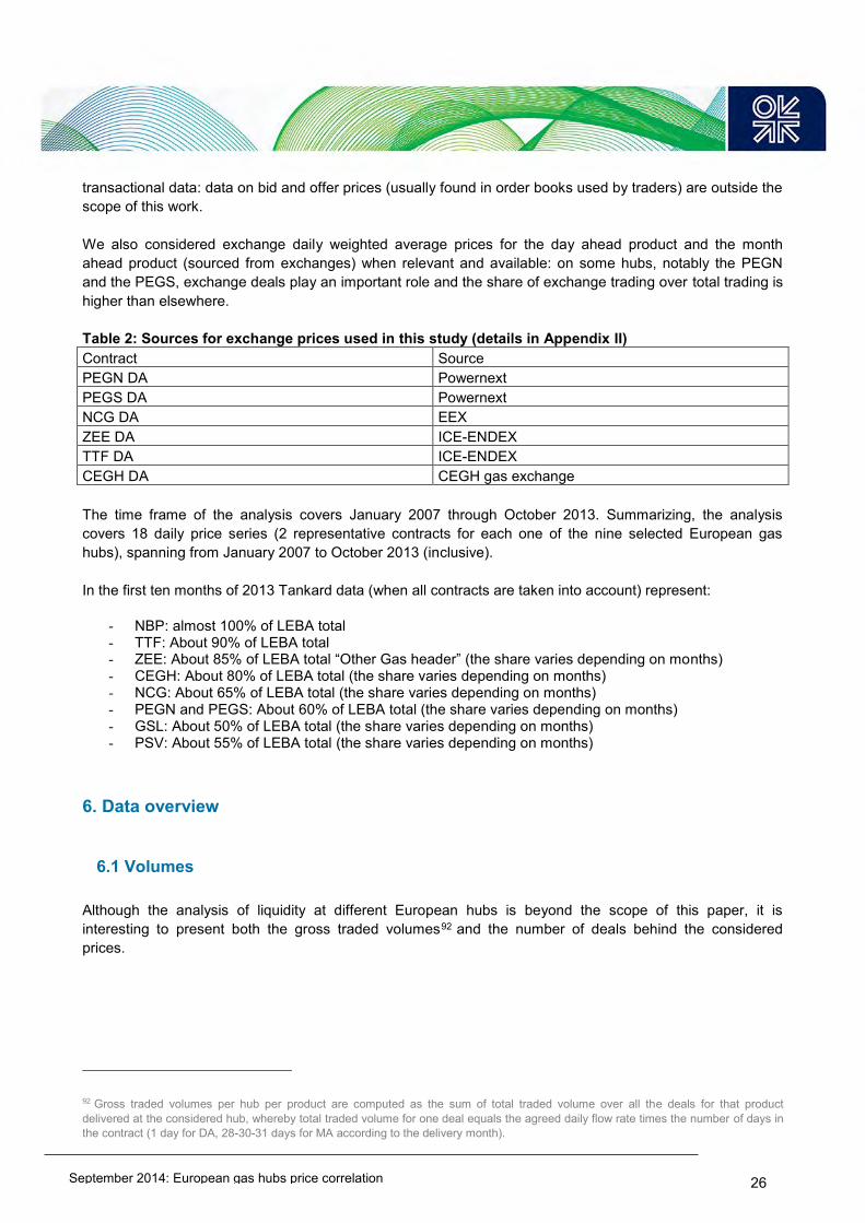
September 2014: European gas hubs price correlation
26
transactional data: data on bid and offer prices (usually found in order books used by traders) are outside the scope of this work. We also considered exchange daily weighted average prices for the day ahead product and the month ahead product (sourced from exchanges) when relevant and available: on some hubs, notably the PEGN and the PEGS, exchange deals play an important role and the share of exchange trading over total trading is higher than elsewhere. Table 2: Sources for exchange prices used in this study (details in Appendix II) Contract Source PEGN DA Powernext PEGS DA Powernext NCG DA EEX ZEE DA ICE-ENDEX TTF DA ICE-ENDEX CEGH DA CEGH gas exchange The time frame of the analysis covers January 2007 through October 2013. Summarizing, the analysis covers 18 daily price series (2 representative contracts for each one of the nine selected European gas hubs), spanning from January 2007 to October 2013 (inclusive). In the first ten months of 2013 Tankard data (when all contracts are taken into account) represent:
- NBP: almost 100% of LEBA total - TTF: About 90% of LEBA total - ZEE: About 85% of LEBA total “Other Gas header” (the share varies depending on months) - CEGH: About 80% of LEBA total (the share varies depending on months) - NCG: About 65% of LEBA total (the share varies depending on months) - PEGN and PEGS: About 60% of LEBA total (the share varies depending on months) - GSL: About 50% of LEBA total (the share varies depending on months) - PSV: About 55% of LEBA total (the share varies depending on months)
6. Data overview
6.1 Volumes Although the analysis of liquidity at different European hubs is beyond the scope of this paper, it is interesting to present both the gross traded volumes92 and the number of deals behind the considered prices.
92 Gross traded volumes per hub per product are computed as the sum of total traded volume over all the deals for that product delivered at the considered hub, whereby total traded volume for one deal equals the agreed daily flow rate times the number of days in the contract (1 day for DA, 28-30-31 days for MA according to the delivery month).

September 2014: European gas hubs price correlation
27
Figure 5: OTC DA traded volumes (TWh)
Note: 2013 data is only for January to October Source: Tankard Parties, author’s analysis In 2012 and 2013 OTC day ahead trading remained very concentrated: in 2012 35% of total annual OTC DA volumes over the 9 selected hubs were traded at NBP, and 22% at TTF; in 201393 these shares were 35% and 28% respectively. NCG ranks third in terms of OTC DA volumes (NCG OTC DA volumes overtook ZEE ones in 2010), but volumes at the German hub remain broadly half those at the Dutch hub. TTF almost caught up with NBP, when considering OTC day ahead trading. In 201394 and in 2012 NBP DA volumes traded on the OTC markets remained stable at the 2011 level, while TTF DA volumes in the first ten months of 2013 grew by over 55% compared to the same period of 2012. In general, all the Continental hubs, but for PEG and ZEE, exhibit a sustained growth from 2007 to 201395. ZEE day ahead trading on the OTC markets was stable in 2011 and 2012, although, it recovered in 2013 (cumulated volumes until October 2013 grew by over +30% compared to the first ten months of 2012). In 2012 four hubs experienced a drop in OTC DA volumes: the French PEGs and two German hubs. However, while GSL and NCG recovered in 2013 totalling in October 50 TWh and almost 125 TWh respectively, PEG DA volumes declined in 2013 (-12% Jan-Oct 12 on Jan-Oct 13). This decrease concerned both the more liquid PEGN and the PEGS and may be related to the recent diversion of LNG towards the more profitable Asian markets96. In 2013 PSV DA volumes boomed and in October totalled almost 6 TWh, a marginal figure compared to other hubs (this is 2% of TTF corresponding volumes) but still over 15 times the figure for 2012. 93 Up to October 2013. 94 Up to October 2013. 95 Up to October 2013. 96 See discussion in Chapter 7.
0
20
40
60
80
100
120
140
2007 2008 2009 2010 2011 2012 2013
TWh
ZEE NCG GSL PEG CEGH PSV
0
50
100
150
200
250
300
350
2007 2008 2009 2010 2011 2012 2013
NBP TTF
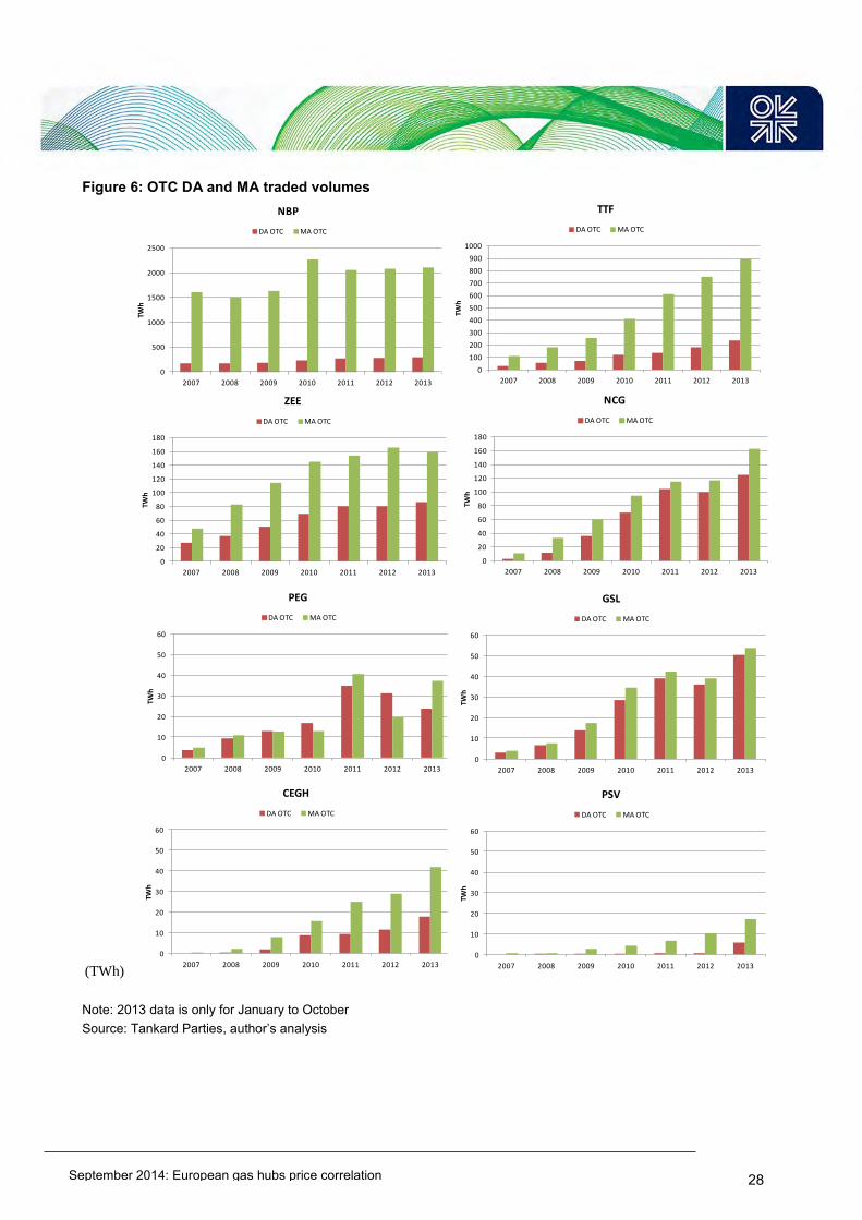
September 2014: European gas hubs price correlation
28
Figure 6: OTC DA and MA traded volumes
(TWh)
Note: 2013 data is only for January to October Source: Tankard Parties, author’s analysis
0
500
1000
1500
2000
2500
2007 2008 2009 2010 2011 2012 2013
TWh
NBP
DA OTC MA OTC
0
20
40
60
80
100
120
140
160
180
2007 2008 2009 2010 2011 2012 2013
TWh
ZEE
DA OTC MA OTC
0
100
200
300
400
500
600
700
800
900
1000
2007 2008 2009 2010 2011 2012 2013
TWh
TTF
DA OTC MA OTC
0
10
20
30
40
50
60
2007 2008 2009 2010 2011 2012 2013
TWh
PEG
DA OTC MA OTC
0
10
20
30
40
50
60
2007 2008 2009 2010 2011 2012 2013
TWh
GSL
DA OTC MA OTC
0
20
40
60
80
100
120
140
160
180
2007 2008 2009 2010 2011 2012 2013
TWh
NCG
DA OTC MA OTC
0
10
20
30
40
50
60
2007 2008 2009 2010 2011 2012 2013
TWh
CEGH
DA OTC MA OTC
0
10
20
30
40
50
60
2007 2008 2009 2010 2011 2012 2013
TWh
PSV
DA OTC MA OTC

September 2014: European gas hubs price correlation
29
OTC month ahead trading remained even more concentrated than DA trading: in 2012 60% of total annual OTC DA volumes over the 9 selected hubs were traded at NBP, and 22% at TTF; in 201397 these shares were 61% and 26% respectively. TTF is approaching NBP in terms of traded volumes, NBP OTC MA volumes stabilized around the 2011 level, while TTF volumes were still growing at a pace of around 20% year on year. In 201398 NCG ranked third and overtook ZEE in terms of OTC month ahead trading, reaching around 160 TWh, which is less than the 20% of TTF volumes in the same year though. TTF, the German hubs, CEGH and PSV overall grew at a sustained rate from 2007 up to 2013. When looking at MA volumes; in 201399 PEG volumes recovered compared to 2012 (in October 2013 cumulative OTC MA volumes more than doubled the figure for the first 10 months of 2012), in contrast to the decline in DA trade. In the course of the process relating to the Target Model Update, ACER defined the concept of the price relevance threshold, that is the minimum number of deals required per product/hub/trading-day in order for price signals to be considered trustworthy. Following a questionnaire100 ACER observed that this minimum number of deals required per product/hub/trading-day should be 18. Based on this, as an indicator for the relevance of considered daily VWAPs, we examined the % of days in our sample in which the number of deals/prod/hub/trading day is higher than 18. Table 3: % of trading days when n. deals/product/hub >= 18 (OTC DA) by year
NBP TTF ZEE NCG GSL CEGH PEGN PEGS PSV 2007 100% 99% 72% 8% 3% 0% 0% 0% 0% 2008 100% 100% 98% 97% 26% 2% 52% 2% 2% 2009 100% 100% 98% 100% 88% 5% 82% 2% 2% 2010 100% 100% 100% 100% 100% 67% 68% 3% 2% 2011 100% 100% 100% 100% 100% 67% 100% 9% 3% 2012 100% 100% 100% 100% 100% 85% 100% 30% 6% 2013 100% 100% 100% 100% 100% 99% 95% 23% 36%
Note: 2013 data is only for January to October Source: Tankard Parties, author’s analysis
97 Up to October 2013. 98 Up to October 2013. 99 Up to October 2013. 100 In this questionnaire one of the question was “How many deals for a specific gas forward product (e.g. a specific quarter or season for a specific hub) need to be concluded on a single trading day so that you would consider the price signal generated on the basis of these deals as trustworthy?” It is not specified whether this indicator include both OTC and exchange deals.

September 2014: European gas hubs price correlation
30
Table 4: Average n. deals/product/hub (OTC DA) by year NBP TTF ZEE NCG GSL CEGH PEGN PEGS PSV
2007 172 84 24 8 6 0 7 0 0 2008 181 133 34 44 13 0 19 1 0 2009 173 151 40 94 28 5 29 5 0 2010 215 214 57 146 55 22 31 2 1 2011 255 205 68 179 63 22 57 10 1 2012 320 276 83 172 61 31 57 14 2 2013 314 280 108 206 88 46 51 13 15
Note: 2013 data is only for January to October Source: Tankard Parties, author’s analysis Considering our sample, in 2013 the number of days in which the number of deals > 18 is below one third in PEGS and PSV, while it is above 95% for all the others. However if we consider DA exchange trades the picture slightly improves for the PEGS. The average number of DA deals for delivery at PEGS concluded through Powernext is 18 in January-October 2013 (the same figure was 13 for OTC) and the share of days in which n° of deals > 18 rises from 23% to about 40%. When turning to PSV, DA exchange deals (GME MGP GAS) concluded in 2013 were only 4101. Table 5: % of trading days when n. deals/product/hub/year >= 18 (OTC MA)
NBP TTF ZEE NCG GSL CEGH PEGN PEGS PSV
2007 100% 40% 1% 0% 0% 0% 0% 0% 0% 2008 102% 74% 7% 4% 2% 2% 2% 2% 2% 2009 102% 93% 12% 12% 2% 2% 2% 2% 2% 2010 102% 100% 17% 34% 4% 2% 2% 2% 2% 2011 103% 103% 37% 41% 6% 3% 5% 3% 3% 2012 106% 106% 40% 42% 9% 7% 7% 6% 6% 2013 100% 100% 30% 56% 9% 4% 2% 0% 0%
Note: 2013 data is only for January to October Source: Tankard Parties, author’s analysis
101 GME (2014), P.86.

September 2014: European gas hubs price correlation
31
Table 6: Average n. deals/product/hub/year (OTC MA) NBP TTF ZEE NCG GSL CEGH PEGN PEGS PSV
2007 224 18 4 2 1 0 1 0 0 2008 223 28 7 5 1 0 1 0 0 2009 230 39 9 9 2 1 2 0 0 2010 305 64 11 14 5 2 1 0 0 2011 269 92 15 17 6 3 4 0 1 2012 294 111 15 17 5 3 2 1 1 2013 239 110 15 22 7 6 3 1 2
Note: 2013 data is only for January to October Source: Tankard Parties, author’s analysis
6.2 Prices The evolution of OTC DA prices for each hub in 2012-2013 is illustrated in Figure 7. A comparison between most recent data and past years is offered by the box plot; complete daily prices time series for each hub are in Appendix I. Figure 7: OTC DA prices in 2012 and 2013 (€/MWh)
Source: Tankard Parties, author’s analysis
20
22
24
26
28
30
32
34
36
38
40
02
-Ja
n-1
2
16
-Ja
n-1
2
30
-Ja
n-1
2
13
-Feb
-12
27
-Feb
-12
12
-Ma
r-1
2
26
-Ma
r-1
2
11
-Ap
r-1
2
25
-Ap
r-1
2
09
-Ma
y-1
2
23
-Ma
y-1
2
07
-Ju
n-1
2
21
-Ju
n-1
2
05
-Ju
l-1
2
19
-Ju
l-1
2
02
-Au
g-1
2
16
-Au
g-1
2
30
-Au
g-1
2
13
-Sep
-12
27
-Sep
-12
11
-Oct
-12
25
-Oct
-12
08
-No
v-1
2
22
-No
v-1
2
06
-Dec
-12
20
-Dec
-12
08
-Ja
n-1
3
22
-Ja
n-1
3
05
-Feb
-13
19
-Feb
-13
05
-Ma
r-1
3
19
-Ma
r-1
3
04
-Ap
r-1
3
18
-Ap
r-1
3
02
-Ma
y-1
3
16
-Ma
y-1
3
31
-Ma
y-1
3
14
-Ju
n-1
3
28
-Ju
n-1
3
12
-Ju
l-1
3
26
-Ju
l-1
3
09
-Au
g-1
3
23
-Au
g-1
3
09
-Sep
-13
23
-Sep
-13
07
-Oct
-13
21
-Oct
-13
NBP ZEE TTF GSL NCG CEGH PSV PEGN PEGS
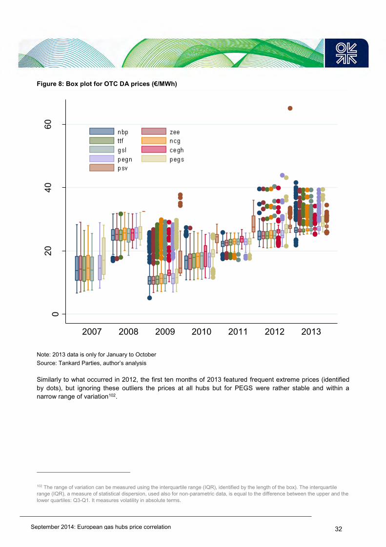
September 2014: European gas hubs price correlation
32
Figure 8: Box plot for OTC DA prices (€/MWh)
Note: 2013 data is only for January to October Source: Tankard Parties, author’s analysis Similarly to what occurred in 2012, the first ten months of 2013 featured frequent extreme prices (identified by dots), but ignoring these outliers the prices at all hubs but for PEGS were rather stable and within a narrow range of variation102.
102 The range of variation can be measured using the interquartile range (IQR), identified by the length of the box). The interquartile range (IQR), a measure of statistical dispersion, used also for non-parametric data, is equal to the difference between the upper and the lower quartiles: Q3-Q1. It measures volatility in absolute terms.
020
4060
2007 2008 2009 2010 2011 2012 2013
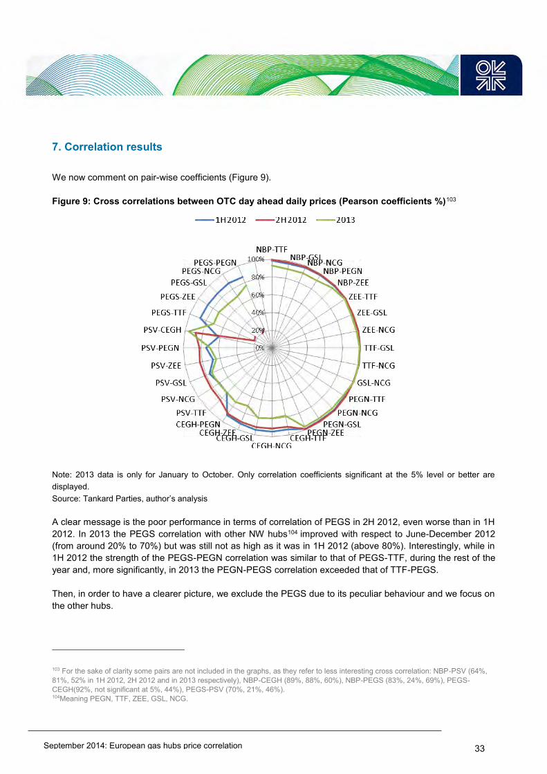
September 2014: European gas hubs price correlation
33
7. Correlation results We now comment on pair-wise coefficients (Figure 9). Figure 9: Cross correlations between OTC day ahead daily prices (Pearson coefficients %)103
Note: 2013 data is only for January to October. Only correlation coefficients significant at the 5% level or better are displayed. Source: Tankard Parties, author’s analysis A clear message is the poor performance in terms of correlation of PEGS in 2H 2012, even worse than in 1H 2012. In 2013 the PEGS correlation with other NW hubs104 improved with respect to June-December 2012 (from around 20% to 70%) but was still not as high as it was in 1H 2012 (above 80%). Interestingly, while in 1H 2012 the strength of the PEGS-PEGN correlation was similar to that of PEGS-TTF, during the rest of the year and, more significantly, in 2013 the PEGN-PEGS correlation exceeded that of TTF-PEGS. Then, in order to have a clearer picture, we exclude the PEGS due to its peculiar behaviour and we focus on the other hubs.
103 For the sake of clarity some pairs are not included in the graphs, as they refer to less interesting cross correlation: NBP-PSV (64%, 81%, 52% in 1H 2012, 2H 2012 and in 2013 respectively), NBP-CEGH (89%, 88%, 60%), NBP-PEGS (83%, 24%, 69%), PEGS-CEGH(92%, not significant at 5%, 44%), PEGS-PSV (70%, 21%, 46%). 104Meaning PEGN, TTF, ZEE, GSL, NCG.
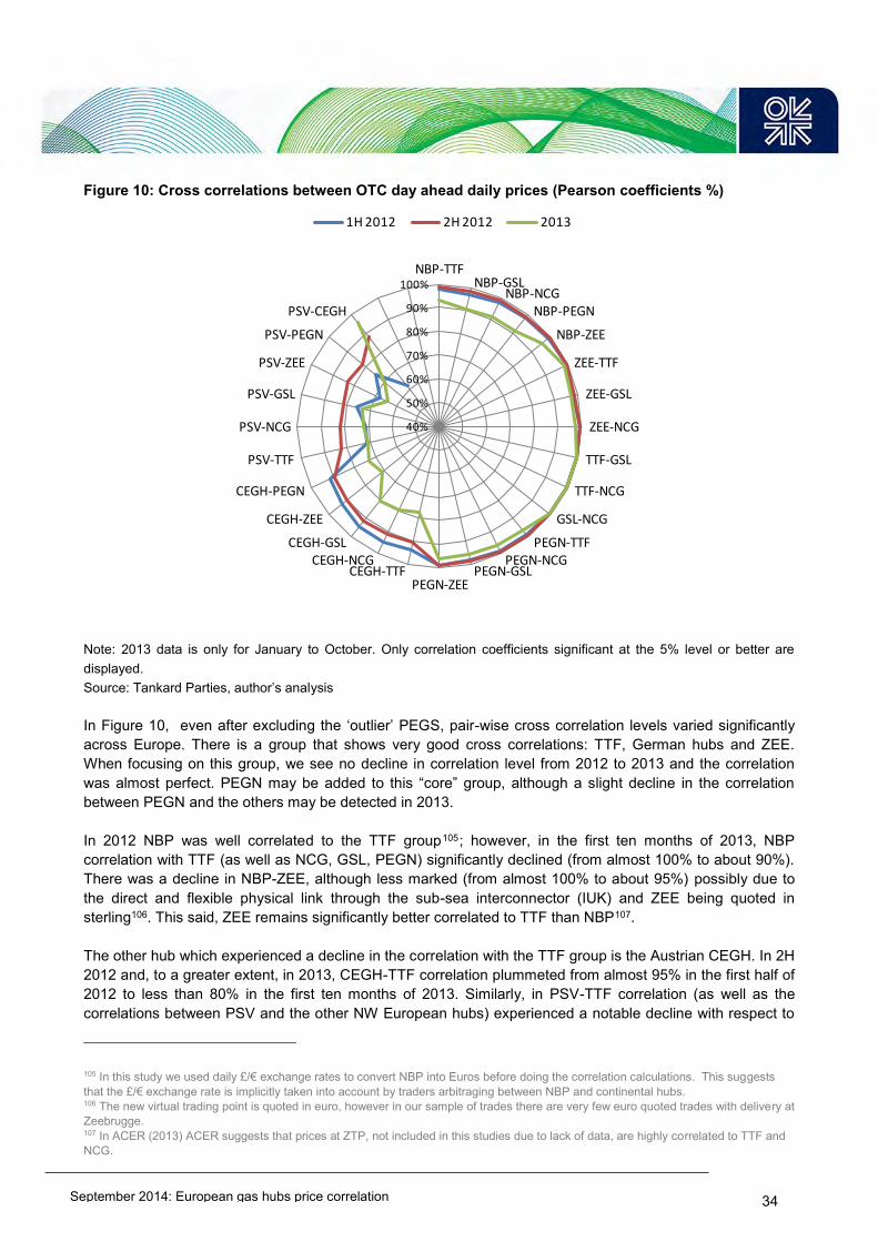
September 2014: European gas hubs price correlation
34
Figure 10: Cross correlations between OTC day ahead daily prices (Pearson coefficients %)
Note: 2013 data is only for January to October. Only correlation coefficients significant at the 5% level or better are displayed. Source: Tankard Parties, author’s analysis In Figure 10, even after excluding the ‘outlier’ PEGS, pair-wise cross correlation levels varied significantly across Europe. There is a group that shows very good cross correlations: TTF, German hubs and ZEE. When focusing on this group, we see no decline in correlation level from 2012 to 2013 and the correlation was almost perfect. PEGN may be added to this “core” group, although a slight decline in the correlation between PEGN and the others may be detected in 2013. In 2012 NBP was well correlated to the TTF group105; however, in the first ten months of 2013, NBP correlation with TTF (as well as NCG, GSL, PEGN) significantly declined (from almost 100% to about 90%). There was a decline in NBP-ZEE, although less marked (from almost 100% to about 95%) possibly due to the direct and flexible physical link through the sub-sea interconnector (IUK) and ZEE being quoted in sterling106. This said, ZEE remains significantly better correlated to TTF than NBP107. The other hub which experienced a decline in the correlation with the TTF group is the Austrian CEGH. In 2H 2012 and, to a greater extent, in 2013, CEGH-TTF correlation plummeted from almost 95% in the first half of 2012 to less than 80% in the first ten months of 2013. Similarly, in PSV-TTF correlation (as well as the correlations between PSV and the other NW European hubs) experienced a notable decline with respect to
105 In this study we used daily £/€ exchange rates to convert NBP into Euros before doing the correlation calculations. This suggests that the £/€ exchange rate is implicitly taken into account by traders arbitraging between NBP and continental hubs. 106 The new virtual trading point is quoted in euro, however in our sample of trades there are very few euro quoted trades with delivery at Zeebrugge. 107 In ACER (2013) ACER suggests that prices at ZTP, not included in this studies due to lack of data, are highly correlated to TTF and NCG.
40%
50%
60%
70%
80%
90%
100%NBP-TTF
NBP-GSLNBP-NCG
NBP-PEGN
NBP-ZEE
ZEE-TTF
ZEE-GSL
ZEE-NCG
TTF-GSL
TTF-NCG
GSL-NCG
PEGN-TTFPEGN-NCG
PEGN-GSLPEGN-ZEE
CEGH-TTFCEGH-NCG
CEGH-GSL
CEGH-ZEE
CEGH-PEGN
PSV-TTF
PSV-NCG
PSV-GSL
PSV-ZEE
PSV-PEGN
PSV-CEGH
1H 2012 2H 2012 2013

September 2014: European gas hubs price correlation
35
2H 2012, when it achieved a level of more than 80%. As a result of this, in 2013 it was back to the level it was at in the first half of 2012 (around 70%). However, the PSV-CEGH correlation improved from 2012 to 2013: from around 60% in the Jan-June 2012 period, to almost 90% in the rest of 2012 and reached 96% in the first ten months of 2013. Interestingly, in 2013 PSV was far better correlated to CEGH than TTF (96% versus 71%), the crossover occurred in 2H 2012 but was less evident (88% versus 83%) in this specific period. Note that the situation was the opposite in 1H 2012 when TTF-PSV scored 72% and CEGH-PSV 62%.
Group coefficients confirm these findings (Figure 11). Figure 11: Group correlations between OTC day ahead daily prices (Pearson coefficients %)
Note: 2013 data is only for January to October. Source: Tankard Parties, author’s analysis The overall group correlation score declines from 1H 2012 to 2H2012 and did not improve in 2013. This said, the 80% correlation score shown by more recent data may be still considered a good one, even if lower than the 89% achieved in 1H 2012. The good overall score might be explained by the likelihood that a reasonable share of contracted gas in Europe has now some form of TTF indexation108. However, although 80% overall remains a good result, correlation is considerably higher when considering sub-groups. In fact, the exclusion of some hubs results in a significant increase (by over 2 percentage points) in the overall score, notably: PSV in all the considered periods, PEGS since 2H 2012, NBP and CEGH in 2013. Excluding the PEGS from the group had virtually no impact in 1H 2012, while in more recent data it results in a notable increase in group correlation: in 2H 2012 group correlation jumps from 81% to 93% and in 2013 from 80% to 85%. The removal of the PSV from the group improves correlation by 5 percentage points in 2H 2012 as well as in 2013, a less strong impact than in 1H 2012, signalling that the impact of PSV on group correlation was less
108See for instance Natural gas contract renegotiation trend boosts spot market volumes, ICIS Heren ,July, 7 2014 available at : http://www.icis.com/resources/news/2014/07/07/9798903/natural-gas-contract-renegotiation-trend-boosts-spot-market-volumes/
89%90%
97%99% 99% 99% 100%
81%
93%
97%
99% 99% 99% 100%
80%
85%
90%
96%98% 99% 99%
40%
50%
60%
70%
80%
90%
100%
all all wo PEGS all wo PEGS and PSV all wo PSV, PEG Sud andCEGH
all wo PSV, PEG Sud,CEGH and NBP
all wo PSV, PEG Sud,CEGH, NBP and PEGN
all wo PSV, PEG Sud,CEGH, NBP, PEGN and ZEE
1H 2012 2H 2012 2013

September 2014: European gas hubs price correlation
36
detrimental in more recent data. The strength of the correlation between Continental hubs excluding PSV and PEGS slightly decreases in 2013 compared to 2012. This is partially due to the already mentioned decline in CEGH correlation coefficients: the exclusion of CEGH allows for a growth of 6 percentage points in the score of the Continental hubs+NBP group. Note that this was not the case in 2012, when the impact of CEGH on group correlation was less detrimental. The exclusion of the British hub from the group, which did not improved group correlation in 2012, in 2013 resulted in a better group correlation score, and this signals the above-mentioned decline in correlation experienced by NBP in the first 10 months of 2013. Similarly, although to a lesser extent, excluding PEGN from the Continental hubs group impacts the correlation score more in 2013 than in 2012, this is a sign of a possible decline in PEGN correlation, which has been already mentioned. Summarising, in most recent data PSV, PEGS, NBP and CEGH proved to be somehow less correlated to the others in 2013. In contrast, TTF, NCG, GSL, ZEE and, although to a lesser extent, PEGN remained very strongly correlated. The same changes in correlation from 2012 to 2013 can be found also when assessing MA correlation scores. Figure 12: Cross correlations between OTC month ahead daily prices (Pearson coefficients %)109
Note: 2013 data is only for January to October. Only correlation coefficients significant at the 5% level or better are displayed. Source: Tankard Parties, author’s analysis
109 For the sake of clarity some pairs are not included in the graphs, as they refer to less interesting cross correlation: NBP-PSV (64%, 81%, 52% in 1H 2012, 2H 2012 and in 2013 respectively), NBP-CEGH (89%, 88%, 60%), NBP-PEGS (83%, 24%, 69%), PEGS-CEGH(92%, not significant at 5%, 44%), PEGS-PSV (70%, 21%, 46%).

September 2014: European gas hubs price correlation
37
3 pm VWAP are very similar to daily VWAP scores except for the PEGS, arguably due to the lower number of observations. Due to this similarity, 3 pm VWAP led to almost identical findings as daily VWAP. One minor difference is that using 3pm data leads to some decline in correlation (1-2%) for PEGN, PSV and CEGH, compared to daily price data. Note that the comparison is partially limited because there were not enough observations in 1H 2012 in order to compute the 3pm correlation for all the hubs.
Figure 13: Cross correlations between OTC day ahead 3 pm WVAP and OTC DA daily prices (Pearson coefficients %)
Note: 2013 data is only for January to October. Only correlation coefficients significant at the 5% level or better are displayed. Source: Tankard Parties, author’s analysis 3pm scores nonetheless confirm the strong link between the “core group”, the 10% decline in correlation between CEGH and other North West Europe hubs (TTF, GSL, NCG, ZEE, PEGN) , the decline in correlation between PSV and TTF (as well as NCG, GSL, ZEE and PEGN), the good and increasing PSV-CEGH correlation in 2013, the slight decline in PEGN-TTF/other NEW hubs in 2013, the decline of NBP-TTF correlation in most recent data.
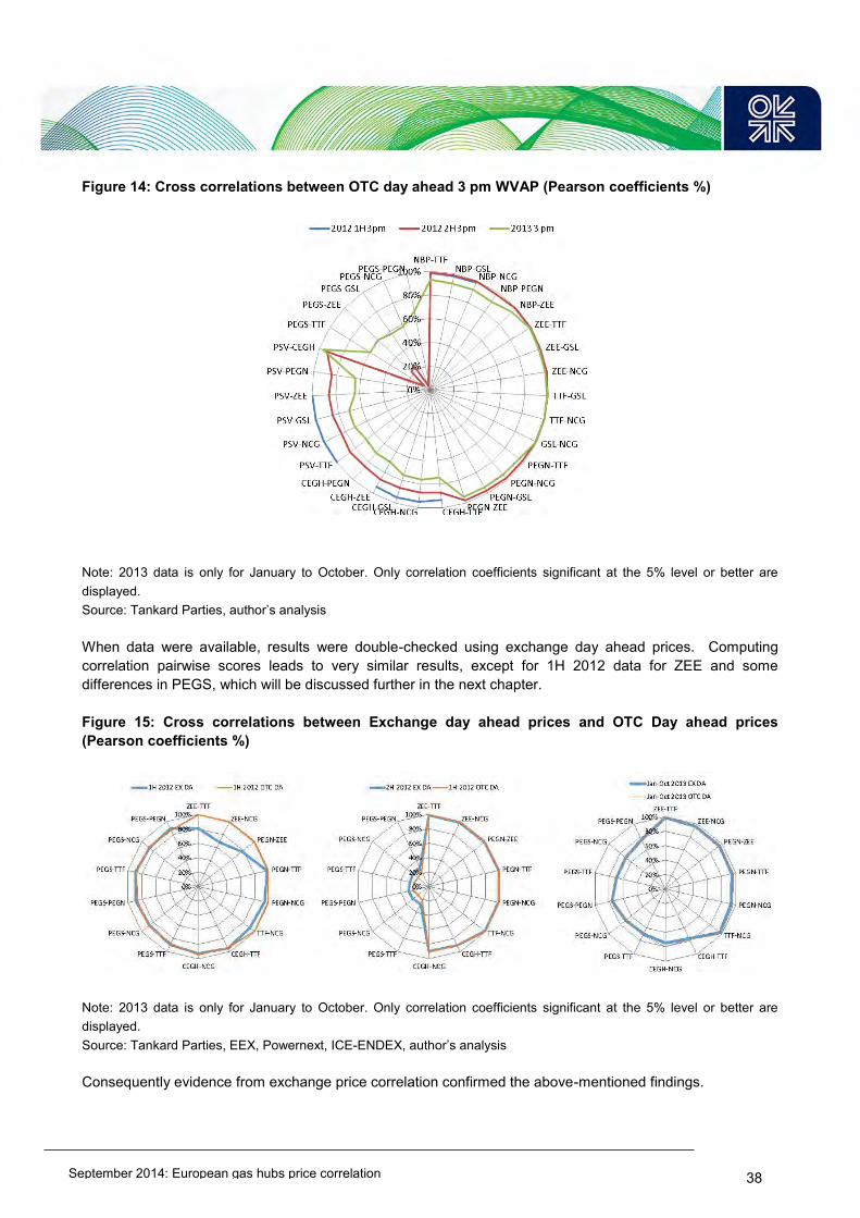
September 2014: European gas hubs price correlation
38
Figure 14: Cross correlations between OTC day ahead 3 pm WVAP (Pearson coefficients %)
Note: 2013 data is only for January to October. Only correlation coefficients significant at the 5% level or better are displayed. Source: Tankard Parties, author’s analysis When data were available, results were double-checked using exchange day ahead prices. Computing correlation pairwise scores leads to very similar results, except for 1H 2012 data for ZEE and some differences in PEGS, which will be discussed further in the next chapter. Figure 15: Cross correlations between Exchange day ahead prices and OTC Day ahead prices (Pearson coefficients %)
Note: 2013 data is only for January to October. Only correlation coefficients significant at the 5% level or better are displayed. Source: Tankard Parties, EEX, Powernext, ICE-ENDEX, author’s analysis Consequently evidence from exchange price correlation confirmed the above-mentioned findings.

September 2014: European gas hubs price correlation
39
Figure 16: Cross correlations between Exchange day ahead prices (Pearson coefficients %)
Note: 2013 data is only for January to October. Only correlation coefficients significant at the 5% level or better are displayed. Source: Tankard Parties, EEX, Powernext, ICE-ENDEX, author’s analysis
7.1 Volatility Correlation As mentioned above, it is important to check the robustness of our finding by looking at return110 or volatility correlation as well. Figure 17: Cross correlations between OTC day ahead daily price returns (Pearson coefficients %)
Note: 2013 data is only for January to October. Only correlation coefficients significant at the 5% level or better are displayed. Source: Tankard Parties, author’s analysis
110 As explained above, returns is one approach to volatility measurement.

September 2014: European gas hubs price correlation
40
Figure 18: Group correlations between OTC day ahead daily price returns (Pearson coefficients %)
Note: 2013 data is only for January to October. Only correlation coefficients significant at the 5% level or better are displayed. Source: Tankard Parties, author’s analysis Using daily price returns leads to lower correlation scores, except for PSV in 1H 2012 and PEGS in 2H 2012, a fact that may be influenced by the relatively lower number of trades per day in these less liquid markets. Lower correlation scores were expected as correlation between hub price volatilities (rather than between price levels) is a stricter condition. In fact daily price levels may move together because of common trends, but have not perfectly aligned daily price changes. Figure 19: Cross correlations between OTC day ahead daily price returns and OTC DA price levels (Pearson coefficients %)
Note: 2013 data is only for January to October. Only correlation coefficients significant at the 5% level or better are displayed. Source: Tankard Parties, author’s analysis

September 2014: European gas hubs price correlation
41
However, volatility correlation scores are rather good and support the hypothesis of –at least- some of these hubs being a single market: shocks to supply or demand from any location in the market cause similar price changes at all k locations. Moreover, although showing a different order of magnitude, volatility correlation scores are consistent with the main findings mentioned above:
the strong link between TTF, NCG, GSL and, to a lesser extent, ZEE: pairs including these hubs show correlation coefficients above 80% in the considered period;
the decline in correlation between CEGH – other North West Europe (NEW) hubs, anticipated in 2H 2012;
the decline in correlation between PSV – other NWE hubs, anticipated in 2H 2012; the good and increasing PSV-CEGH correlation in 2013, which is higher than the PSV-TTF one and
PSV-NCG. the slight decline in PEGN-TTF/other NWE hubs, anticipated in 2H 2012 and more marked in 2013; the decline of NBP-Continental hubs correlation in most recent data.
Having provided some support for our findings, which surmise that ‘something has changed’ in the most recent data, changes in correlation from 2012 to 2013 will be discussed further below.
7.2 Changes in Correlation Summing up, the analysis of pair-wise and group correlation coefficients highlighted some interesting changes in correlation with respect to the situation in 1H 2012:
1) PEGS delinks significantly in 2H 2012, improves correlation in 2013 but is not back to the levels it achieved in the beginning of 2012.
2) PEGN correlation to TTF (as well as NCG, GSL and ZEE) slightly declines in 2013 and the correlation between the Northern and Southern French hubs strengthens in 2013.
3) CEGH correlation to other NW Continental hubs declines in 2H 2012 and, to a greater extent, in 2013.
4) PSV-TTF correlation first improves in 2H 2012 but then in 2013 is down again at 1H 2012 levels; during the same period PSV-CEGH correlation instead increases and becomes strong in 2013.
5) NBP correlation with TTF (as well as ZEE, NCG, GSL, PEGN) significantly declined in 2013 compared to 2012.
We now discuss each of these changes.
7.3 PEGS As opposed to 1Q 2012, from April 2012 the evolution of prices on PEGS became quite unrelated to all other hubs, in particular during the spring/summer period (Figure 20). During the winter of 2012/2013 PEGS followed more closely the other hubs, but from February 2013 spreads grew again and prices in the South of France did not move in line with those in the rest of North West Europe.

September 2014: European gas hubs price correlation
42
Figure 20: OTC Day ahead prices on TTF, PEG Sud (PEGS) and PEG Nord (PEGN), 2012-2013 (€/MWh)
Source: Tankard Parties and author’s analysis As a result, correlation between PEGN and PEGS decreased remarkably in 2H2012; in 2013 it improves but it was not at the level it was in 1H 2012. During 2013 the correlation between the two French markets dropped from 77% in 1Q down to less than 60% in 3Q (Figure 21). Additionally, while in 1H 2012 the strength of PEGS-PEGN correlation was rather similar to that of PEGS-TTF, during the rest of the year and, more significantly, in 2013 the PEGN-PEGS correlation often exceeded that of TTF-PEGS. Figure 21: Pearson correlation coefficients (%)
Source: Tankard Parties, author’s analysis Those correlation coefficients do not appear to be biased by the presence of outliers, as shown in the scatterplot.
20
22
24
26
28
30
32
34
36
38
40
dapricettf dapricepegn dapricepegs

September 2014: European gas hubs price correlation
43
Figure 22: Scatterplot OTC Day ahead prices – PEGS and PEGN
Source: Tankard Parties, author’s analysis However, OTC trading should not be the only evidence to evaluate when drawing conclusions on the French hubs correlation: when it comes to the French market it is important to verify whether findings hold true also when using Powernext spot exchange data. In fact, in France the share of exchange trades is quite large compared to other markets 111 and Powernext prices are often the reference point for the French gas market112. In addition the drop in OTC DA traded volumes in France led to exchange trading overtaking brokered trading in 2013 (Figure 23).
Figure 23: Traded volume on PEGN and PEGS, DA contract (TWh)
Source: Tankard Parties, Powernext, author’s analysis 111 Petrovich (2013) 112The French Energy Regulator (CRE), for instance, closely monitors Powernext prices. Using Powernext data it draws similar conclusions on PEGS de-linkage. Source: Resolution of the French Energy Regulatory Commission (CRE) dated 29 May 2013 on the formation of gas prices in the South of France, p.1, available at: http://www.cre.fr/en/documents/deliberations/communication/formation-of-gas-prices-in-the-south-of-france

September 2014: European gas hubs price correlation
44
Despite the above-mentioned differences in traded volumes, we expect minor differences between OTC and exchange prices, at least for PEGN given the reasonable volume of trades. Differences may be relevant instead for PEGS where fewer trades are executed. In fact, in the period from January 2012 to October 2013, for the DA contract with delivery at PEGN, the average absolute difference between Powernext and OTC daily prices equals 0.12 €/MWh and on 96% of the days the difference was below 0.5 €/MWh. When turning to PEGS, the average absolute difference is slightly higher (0.32 €/MWh) and the absolute difference was higher than 0.5 €/MWh on 20% of the days during the same period. Figure 24: Frequency distribution for the difference between Powernext and OTC daily prices, DA contract
Source: Tankard Parties, Powernext, author’s analysis Reflecting the similarity between PEGN Powernext and OTC prices, OTC-EX correlation is very good for PEGN: in 2012 it is above 99%, although in the more recent quarters the correlation is down at about 98%. Accordingly, EX-OTC correlation is slightly weaker for PEGS, in particular in 2H 2012 and in 2Q 2013. Figure 25: Correlation coefficients, EX-OTC, DA contract
Source: Tankard Parties, Powernext, author’s analysis This suggests that results obtained using OTC PEGN prices may be easily generalized to Powernext prices as well, while some caution should be adopted when using OTC prices for PEGS. This said, the same
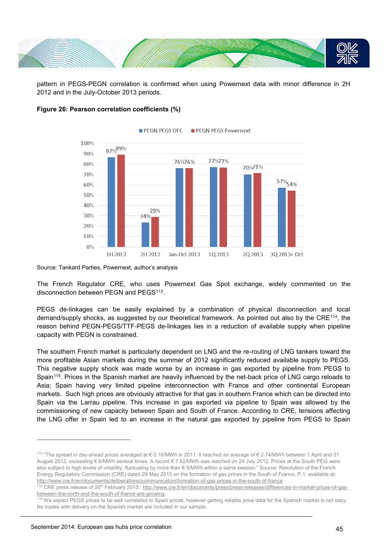
September 2014: European gas hubs price correlation
45
pattern in PEGS-PEGN correlation is confirmed when using Powernext data with minor difference in 2H 2012 and in the July-October 2013 periods. Figure 26: Pearson correlation coefficients (%)
Source: Tankard Parties, Powernext, author’s analysis The French Regulator CRE, who uses Powernext Gas Spot exchange, widely commented on the disconnection between PEGN and PEGS113. PEGS de-linkages can be easily explained by a combination of physical disconnection and local demand/supply shocks, as suggested by our theoretical framework. As pointed out also by the CRE114, the reason behind PEGN-PEGS/TTF-PEGS de-linkages lies in a reduction of available supply when pipeline capacity with PEGN is constrained. The southern French market is particularly dependent on LNG and the re-routing of LNG tankers toward the more profitable Asian markets during the summer of 2012 significantly reduced available supply to PEGS. This negative supply shock was made worse by an increase in gas exported by pipeline from PEGS to Spain115. Prices in the Spanish market are heavily influenced by the net-back price of LNG cargo reloads to Asia; Spain having very limited pipeline interconnection with France and other continental European markets. Such high prices are obviously attractive for that gas in southern France which can be directed into Spain via the Larrau pipeline. This increase in gas exported via pipeline to Spain was allowed by the commissioning of new capacity between Spain and South of France. According to CRE, tensions affecting the LNG offer in Spain led to an increase in the natural gas exported by pipeline from PEGS to Spain
113 “The spread in day-ahead prices averaged at € 0.16/MWh in 2011. It reached an average of € 2.74/MWh between 1 April and 31 August 2012, exceeding € 6/MWh several times. A record € 7.62/MWh was reached on 24 July 2012. Prices at the South PEG were also subject to high levels of volatility, fluctuating by more than € 5/MWh within a same session.” Source: Resolution of the French Energy Regulatory Commission (CRE) dated 29 May 2013 on the formation of gas prices in the South of France, P.1. available at: http://www.cre.fr/en/documents/deliberations/communication/formation-of-gas-prices-in-the-south-of-france 114 CRE press release of 20th February 2013: http://www.cre.fr/en/documents/press/press-releases/differences-in-market-prices-of-gas-between-the-north-and-the-south-of-france-are-growing. 115 We expect PEGS prices to be well correlated to Spain prices, however getting reliable price data for the Spanish market is not easy. No trades with delivery on the Spanish market are included in our sample.

September 2014: European gas hubs price correlation
46
(through the two interconnection points at Larrau and Biriatou), which in turn brought up prices in the South of France. The France-Spain interconnection was used at a very high rate. The impact of exports to Spain on PEGS prices may be demonstrated by the fact that the price spread between PEGN and PEGS dropped significantly during maintenance to the Larrau interconnection from 27 to 31 August and during the strike action at TIGF from 28 September to 2 October 2012116. Following the reduction in Southern France LNG supply and the growing exports to Spain, PEGS was forced to rely on gas coming from the North of France through the GRTgaz North-to-South link. Increasing demand led to the saturation of transportation capacities between the two French zones, especially in summer, when send-out at the Montoir terminal (on the North West French Atlantic coast) heavily reduces the availability of capacity in the North-South link. The French regulator argued that, in summer, send-out at the Montoir terminal heavily reduces the availability of interruptible capacity on the North-South link, as Montoir’s send-out can make up to 190 GWh/day available on the North-to-South link (almost 45% of its technical capacity)117. In addition to the supply tensions in the South of France, CRE has noted a number of specific factors that may have heightened tensions on prices in these zones118. As reported by CRE, the link was saturated for most of the summer of 2012 from North to South, with a 94% rate of use, compared to 61% in 2011. In the first quarter of 2013 the utilization rate of firm capacity reached 94%, while availability rate of interruptible capacity was 44%, compared to 76% observed in 1Q 2012119. The utilization rate of the North-to-South link averaged 97% during Q3 2013120. CRE has undertaken a number of actions to optimise the use of facilities in the short term and set guidelines with a view to merging zones, in order to improve the market conditions in the South of France in the long term121. It is difficult to say whether the North-South congestion is going to persist, it may last until the enlargement of capacity on the North-South link, but supply/demand factors matter as well: a surge of LNG overspill from Asia in the 2018 - 2023 period might resolve the PEGS issue, at least for a while.
7.4 PEGN In 2013 correlation between PEGN and its neighbouring hubs (ZEE and NCG), as well as with TTF, slightly decreased, both when looking at DA and MA. This decline in PEGN correlation in 2013 is not nearly as strong as that of PEGS but is still significant. However, it is worth noting that, while DA prices show a clear decreasing pattern in correlation through January-October 2013 (from 98% and 99% in 1Q 2013 to 88% and 77% in July-October for PEGN-NCG and PEGN-ZEE respectively), there is not a clear negative trend in 2013 when looking at MA prices. This suggests that PEGN and the NWE core group (NCG, ZEE, TTF and GSL) may remain closely correlated in the long run, possibly with TTF being the driver122.
116 Resolution of the French Energy Regulatory Commission (CRE) dated 29 May 2013 on the formation of gas prices in the South of France, p.3. available at: http://www.cre.fr/en/documents/deliberations/communication/formation-of-gas-prices-in-the-south-of-france 117 Resolution of the French Energy Regulatory Commission (CRE) dated 29 May 2013 on the formation of gas prices in the South of France, p.3. available at: http://www.cre.fr/en/documents/deliberations/communication/formation-of-gas-prices-in-the-south-of-france 118 Resolution of the French Energy Regulatory Commission (CRE) dated 29 May 2013 on the formation of gas prices in the South of France. available at: http://www.cre.fr/en/documents/deliberations/communication/formation-of-gas-prices-in-the-south-of-france 119CRE (2013a), P.67. 120CRE (2013c), P.31. 121Resolution of the French Energy Regulatory Commission (CRE) dated 29 May 2013 on the formation of gas prices in the South of France. available at: http://www.cre.fr/en/documents/deliberations/communication/formation-of-gas-prices-in-the-south-of-france 122Petrovich (2013).
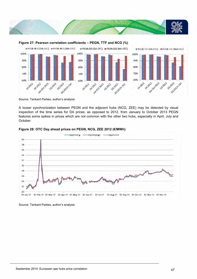
September 2014: European gas hubs price correlation
47
Figure 27: Pearson correlation coefficients – PEGN, TTF and NCG (%)
Source: Tankard Parties, author’s analysis A looser synchronization between PEGN and the adjacent hubs (NCG, ZEE) may be detected by visual inspection of the time series for DA prices: as opposed to 2012, from January to October 2013 PEGN features some spikes in prices which are not common with the other two hubs, especially in April, July and October. Figure 28: OTC Day ahead prices on PEGN, NCG, ZEE 2012 (€/MWh)
Source: Tankard Parties, author’s analysis

September 2014: European gas hubs price correlation
48
Figure 29: OTC Day ahead prices on PEGN, NCG, ZEE in 2013 (€/MWh)
Source: Tankard Parties, author’s analysis Additionally, the median spread between the North of France and Germany rose to about 0.2 €/MWh in January-October 2013, while it was at about 0.1 €/MWh in 2H 2012. In the first 10 months of 2013 the spread of PEGN-NCG also becomes more volatile than in previous months. Figure 30: OTC Day ahead prices, PEGN-NCG spread over time and frequency distribution (€/MWh,%)
Source: Tankard Parties, author’s analysis The price spike occurred on the 10th of April 2013 is the most relevant one. This pushed the premium of PEGN over NCG above 6 €/MWh, a figure which does not fit the general trend.

September 2014: European gas hubs price correlation
49
On this “outlier” day PEGN and PEGS soared, while NCG, ZEE as well as other Continental hubs remained relatively stable. This isolated price spike was caused by supply concerns due to a firm capacity restriction at Dunkirk and the Taisnieres interconnection with Belgium, coupled with temperatures below the seasonal average and low storage levels123. As this day is indeed an exceptional one, not fitting the general trend of observations for 2013, it may lead to an “outlier bias”, distorting downward correlation score, as suggested by the scatterplot. Figure 31: Scatterplot DA OTC prices – PEGN against NCG and PEGN against ZEE
Source: Tankard Parties, author’s analysis If we exclude this “exceptional” day, the correlation score for 2013 increases. Figure 32: Pearson correlation coefficients – PEGN, NCG and ZEE
Source: Tankard Parties, author’s analysis
123Platts Gas Daily Monthly Averages, April 2013, P.2 and CRE (2013b), P.67.

September 2014: European gas hubs price correlation
50
Decline in the correlation PEGN to the rest of Northern Europe seems therefore linked, at least to some extent, to contingent factors (“an exceptional day”) in 2Q 2013. This is not the case for the summer of 2013, though, as we cannot detect such clearly outlying observations. In September 2013 however there is a period in which the spread of PEGN-NCG enlarges and becomes more volatile than in previous months. This was due to the North of France being partially disconnected from NCG (80% of firm capacity interruption at Medelsheim–Obergailbach IP at the France-Germany border), while subject to a reduction in gas supplied from Norway due to a 55% firm capacity interruption at Dunkirk124. We now adopt the more generalized approach illustrated above, aiming at testing whether the decrease in correlation in 2013 may be explained by physical disconnection between PEGN and other NWE hubs. We look for physical pipeline congestion at the DE-FR border, which should affect the NCG-PEGN price correlation, as well as at the BE-FR border, which should affect the ZEE-PEGN price correlation. We therefore consider flows proceeding from NCG and entering the North of France at Obergailbach and flows coming from Belgium and entering France at Taisnieres B and Taisnieres H. Figure 33: Simple representation of PEGN interconnections
Source: Smart GRT gaz website and author 124 Platts Gas Daily Monthly Averages, September 2013, p.1 and CRE (2013c), P.32.

September 2014: European gas hubs price correlation
51
For each relevant IP entry-to-France side, we compute a utilization rate using GRT-gaz data on actual flows entering France and technical effective entry capacity. The latter ranged between 110,000,000 kWh and 675,000,000 kWh in the considered period, with a median value of 640,000,000 kWh. Note that we do not consider the corresponding exit-from-NCG and exit-from-ZEE sides and therefore we assume no bottlenecks on the exit side of the IP. In fact, in the event that entry capacity from Germany/Belgium to France was lower than exit capacity from Germany/Belgium to France, physical congestion at IP may occur even when entry-to-France capacity utilization rate is far below one, provided that exit-from-Germany/Belgium is already saturated. Figure 34: Utilization rate at Obergailbach entry to France, 2012- October 2013 (%)
Source: GRTgaz
Figure 35: Utilization rate at Taisnieres B entry to France, 2012- October 2013 (%)
Source: GRTgaz
0%
20%
40%
60%
80%
100%
120%
Jan
-12
Feb
-12
Mar
-12
Ap
r-1
2
May
-12
Jun
-12
Jul-
12
Au
g-1
2
Sep
-12
Oct
-12
No
v-1
2
Dec
-12
Jan
-13
Feb
-13
Mar
-13
Ap
r-1
3
May
-13
Jun
-13
Jul-
13
Au
g-1
3
Sep
-13
Oct
-13
Utilization rate Obergailbach entry to France
0%
10%
20%
30%
40%
50%
60%
70%
80%
90%
100%
Jan
-12
Feb
-12
Mar
-12
Ap
r-1
2
May
-12
Jun
-12
Jul-
12
Au
g-1
2
Sep
-12
Oct
-12
No
v-1
2
Dec
-12
Jan
-13
Feb
-13
Mar
-13
Ap
r-1
3
May
-13
Jun
-13
Jul-
13
Au
g-1
3
Sep
-13
Oct
-13
Utilization rate Taisnières B entry to France

September 2014: European gas hubs price correlation
52
Figure 36: Utilization rate at Taisnieres H entry to France, 2012- October 2013 (%)
Source: GRTgaz Our analysis shows that when we exclude days in which the utilization rate was either zero or above 0.9 then correlation for 2013 increases. This suggests that at least some de-linkage in 2013 may be the result of lack physical transport capacity. Figure 37: Pearson correlation coefficients between NCG and PEGN over different time periods (%)
. All = all days Wo full = excluding days in which utilization rate was either zero or above 0.9 Source: GRTgaz, Tankard Parties, author’s analysis
0%
10%
20%
30%
40%
50%
60%
70%
80%
90%
100%
Jan
-12
Feb
-12
Mar
-12
Ap
r-1
2
May
-12
Jun
-12
Jul-
12
Au
g-1
2
Sep
-12
Oct
-12
No
v-1
2
Dec
-12
Jan
-13
Feb
-13
Mar
-13
Ap
r-1
3
May
-13
Jun
-13
Jul-
13
Au
g-1
3
Sep
-13
Oct
-13
Utilization rate Taisnières H entry to France
94%
95%
96%
97%
98%
99%
100%
1H2012 2H2012 Jan-Oct 2013
NCG-PEGN all NCG-PEGN wo full
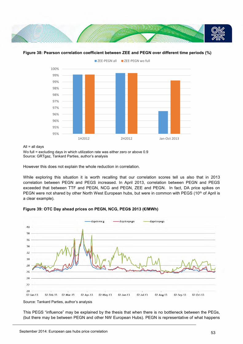
September 2014: European gas hubs price correlation
53
Figure 38: Pearson correlation coefficient between ZEE and PEGN over different time periods (%)
All = all days Wo full = excluding days in which utilization rate was either zero or above 0.9 Source: GRTgaz, Tankard Parties, author’s analysis However this does not explain the whole reduction in correlation. While exploring this situation it is worth recalling that our correlation scores tell us also that in 2013 correlation between PEGN and PEGS increased. In April 2013, correlation between PEGN and PEGS exceeded that between TTF and PEGN, NCG and PEGN, ZEE and PEGN. In fact, DA price spikes on PEGN were not shared by other North West European hubs, but were in common with PEGS (10th of April is a clear example). Figure 39: OTC Day ahead prices on PEGN, NCG, PEGs 2013 (€/MWh)
Source: Tankard Parties, author’s analysis This PEGS “influence” may be explained by the thesis that when there is no bottleneck between the PEGs, (but there may be between PEGN and other NW European Hubs). PEGN is representative of what happens
95%
95%
96%
96%
97%
97%
98%
98%
99%
99%
100%
1H2012 2H2012 Jan-Oct 2013
ZEE-PEGN all ZEE-PEGN wo full
admin
Typewritten Text
admin
Typewritten Text
admin
Typewritten Text

September 2014: European gas hubs price correlation
54
across the entire French market, so some factors which have a significant impact on PEGS may have some impact on PEGN as well (for instance increased demand for LNG in Asia). It may be said that much that happens in France, even in the South, affects prices at PEGN. Moreover PEGS and PEGN are also linked by the fact that LNG terminals in the South of France and those in the North import Algerian gas. Hence any disruptions in Algerian supply affect both PEGS and PEGN. Disruption in Qatari LNG supply instead affects only PEGS. On the basis of data available it has not been possible to prove or disprove the thesis that PEGN is representative of what happens across the entire French market.
7.5 CEGH Turning to CEGH, we see a fairly significant decline in correlation in 2013, almost 10% against the NW hubs. Hereafter we focus on CEGH correlation against TTF, the benchmark hub for Continental European hubs125, and NCG, the adjacent hub to CEGH among the ones considered in this study126. In Q1 2013 there was a slight decline in the CEGH-TTF pair-wise correlation (as well as the NCG-CEGH one) and in summer 2013 correlation scores declined even further. Correlation appeared to be quite good in Q2 2013 however. Figure 40: OTC Day ahead prices on TTF, CEGH and NCG, 2012-2013 (€/MWh)
Source: Tankard Parties, author’s analysis
125 Petrovich (2013). 126 Note that CEGH is indirectly linked to GSL as gas may flow from Germany to Czech Republic and then to Slovakia via the Lanzhot IP and finally from Slovakia to Austria via the Baumgarten IP.

September 2014: European gas hubs price correlation
55
Figure 41: Pearson pair-wise correlation coefficients based on OTC Day ahead prices on TTF, CEGH, NCG (%)
Source: Tankard Parties, author’s analysis
In 2013 data MA correlation falls as well. Interestingly enough, the most significant decline in MA correlation occurs in 2Q 2013 reflecting possibly that trades were pricing differently to gas delivered in subsequent months, including July 2013. Figure 42: Pearson pair-wise correlation coefficients based on OTC Day ahead prices and OTC MA prices on TTF, CEGH (%)
Source: Tankard Parties, author’s analysis

September 2014: European gas hubs price correlation
56
Figure 43: Pearson pair-wise correlation coefficients based on OTC Day ahead prices and OTC MA prices on NCG, CEGH (%)
Source: Tankard Parties, author’s analysis From the beginning of September 2012 to the end of 2012 the spread was very low and from 8/11/2012 to 18/12/2012 the TTF had a small premium on CEGH. In March 2013 low temperatures drove TTF prices up, exceeding the Austrian price; from April 2013 the spread fluctuated around 1 €/MWh. Figure 44: OTC Day ahead prices, CEGH-NCG spread over time and frequency distribution (€/MWh, %)
Source: Tankard Parties, author’s analysis

September 2014: European gas hubs price correlation
57
Figure 45: OTC Day ahead prices, CEGH-TTF spread, frequency distribution (%)
Source: Tankard Parties, author’s analysis We first check whether the decline in 2013 of the NW European Hubs -CEGH correlation is due to outliers. By examining the scatter plots, we observe that dots in 2013 are more widely spread and there are some outlier days, namely the 19-22 March period. Figure 46: OTC Day ahead prices, CEGH-TTF scatterplot (€/MWh)
Figure 47: OTC Day ahead prices, CEGH-NCG scatterplot (€/MWh)
Source: Tankard Parties, author’s analysis As we do not detect other clear outliers in summer 2013, we may say that from July to October 2013 there is a less clear linear relationship between CEGH and the rest of Northern Europe, and this is not linked to special days as in 2Q 2013.
20
25
30
35
40
20 25 30 35 40
TTF
CEGH
1H 2012
20
25
30
20 25 30
TTF
CEGH
2H 2012
20
25
30
35
20 25 30 35
TTF
CEGH
Jan-Oct 201312-22 March
20
25
30
35
20 25 30 35
CEGH
NCG
2013
20
25
30
35
40
20 25 30 35 40
CEGH
NCG
1H 2012
20
25
30
35
20 25 30 35
CEGH
NCG
2H 2012)

September 2014: European gas hubs price correlation
58
Based on our theoretical framework, this evidence suggests that there may be some form of congestion of interconnecting capacity between Austria and the other NW European Hubs – and in particular the adjacent NCG - in the summer 2013 to October 2013 period and in some days in March. As CEGH is physically linked to NCG, we investigated whether this decline in correlation may be explained by CEGH and NCG being physically disconnected. Before presenting this analysis, it is worth mentioning that when comparing 2013 to 2012, some facts should be taken into account:
- In 2013 CEGH changed from being a physical hub to a VTP (virtual trading point) (Figure 48) 127 - In 2013 nominations at CEGH dropped due to the entry fee that has to be paid following the change
to the new system128 - In May 2013 the Slovak TSO Eustream increased Lanzhot entry tariff and this may have prevented
some “indirect” arbitrage between GSL and CEGH129 - In late 2012 Nord Stream was enlarged and changed flows of gas in Europe130.
Figure 48: Change in CEGH system in 2013
Source: CEGH website Following our methodology, we look for some evidence for physical pipeline congestion at the link between NCG and CEGH. The main link between NCG and CEGH is the bidirectional WAG pipeline and Oberkappel is the IP located at the extreme of WAG located on the Germany-Austria border (Figure 49). The other IP located at the Germany-Austria link, Uberackem, was deemed not relevant for this study.
127 Source: http://www.cegh.at/austrian-gas-market-model-2013 128 CEGH presentation April, 23 2013, retrieved at: www.gasconnect.at 129 Slovak transmission system operator Eustream raised the tariff for capacity at Lanzhot at the Slovak-Czech border from €29.36/MWh/day/year to €102.76/MWh/day/year on 2 May 2013, ICIS HEREN ESGM 24 July 2013. See also official documents: Price Decision for 2013 issued by URSO on 2nd of May 2013 and Price Decision issue by URSO on 10th of October 2012 valid till 1st of May 2013 (https://tis.eustream.sk/TIS/#/?nav=gi.trf). 130 Line 1 was completed in June 2011, and gas transport began in mid-November 2011. Construction of Line 2 began in May 2011, and came on stream in October 2012. Source: http://www.nord-stream.com/the-project/

September 2014: European gas hubs price correlation
59
Figure 49: Interconnections between CEGH and NCG and focus on Oberkappel IP
Source: Transparency platform, CEGH, BOG website, author WAG can be used in a flexible way for arbitrage flows. Through WAG Austria can import gas directly from NCG, in addition, gas coming mostly from Russia can also flow through this pipeline in the opposite direction. Gas is typically sold from Austria to NCG in winter and from Germany to Austria in the summer. However Germany-to-Austria border capacity at Oberkappel is lower than Austria-to-Germany border capacity and this can create bottlenecks when sending NCG gas to CEGH131. This disparity between the entry and the exit side is believed to be the cause of the higher premium for CEGH over NCG over the summer132 and this may play a role in the de-linkage observed in Q3 2013. In order to test our hypothesis, historical daily data for WAG pipeline actual flows and available technical capacity at Entry/Exit Oberkappel IP are needed. We could not obtain this set of data, but we suspect that actually there was some congestion preventing arbitrage flows from NCG to CEGH during the summer of 2013. Barriers may have been both physical, fostered by the above-mentioned disparity between the entry and the exit, but also contractual, consistent with the fact that ACER reported some contractual congestion at Austria-Germany border133. Also the Austrian Energy regulator E-control argued that there is a bottleneck
131 International Gas Report Issue 249, May 19,2014, P.6. 132 International Gas Report Issue 249, May 19,2014, P.6. 133 Map in ACER (2014) , P.52

September 2014: European gas hubs price correlation
60
at Oberkappel 134 . Another factor contributing to congestion may be strong Russian flows coming to Continental Europe, crossing Austria and possibly preventing Germany-to-Austria flows. PSV – CEGH correlation will be discussed in the next section.
7.6 PSV Our pairwise results show that PSV/NWE hubs correlation fell significantly in 2013. To analyse this phenomenon, hereafter we focus on PSV correlation against TTF, the benchmark hub for Continental European hubs135, and NCG, a hub, among the ones considered in this study, which is indirectly linked to PSV, via Switzerland. As noticed above, while delinking from NWE hubs, PSV appeared to move more closely to CEGH than TTF: actually since 2H 2012136 PSV/CEGH correlation has been generally stronger than PSV-TTF or PSV-NCG correlation. Figure 50: Pearson pair-wise correlation coefficients based on OTC day ahead prices on TTF, NCG, CEGH and PSV (%)
Source: Tankard Parties, author’s analysis In Q1 2013 the CEGH-PSV correlation was at the highest, presumably because these two markets were less affected by the cold snap hitting Northern Europe at the end of the spring. However from July to October 2013 the gap between the PSV-CEGH correlation score and the PSV-TTF score widened remarkably. The PSV premium significantly fell in 2H2012 and in the beginning of 2013 the spread was very narrow compared to the past. More specifically there was a quite abrupt decrease in the PSV premium to other North West hubs such as the TTF and the NCG in mid-September 2012. Traders suggested that this occurred due to measures allowing more arbitrage activity between Italy and the rest of Europe137. In thisrespect it is worth mentioning that in September 2012 ENI, in response to an antitrust competition inquiry on abuse of market dominance, agreed to free up cross-border capacity on theTENP/Transitgas connecting PSV to North Europe 138 . In July 2013 ENI, the Italian former incumbent, 134 E-Control (2012), P.70-71. 135 Refer to discussion on which is the benchmark hus in Petrovich (2013). 136 We have only 21 observations in for PSV OTC DA in 1H 2012. 137 Platts Gas Daily Monthly Averages, September 2012, P. 1. 138 http://www.icis.com/resources/news/2012/09/07/9593924/italy-s-eni-ups-natural-gas-transport-capacity-offer-to-head-off-antitrust-inquiry/. Official document here: http://www.agcm.it/trasp-statistiche/doc_download/3287-a440chiusura.html.

September 2014: European gas hubs price correlation
61
launched a service allowing flexible access to its unused transport capacity on pipelines bringing gas from other parts or Europe139. While in early spring 2013 day ahead OTC TTF and NCG prices were rapidly escalating above Italian and Austrian prices (possibly also due to better storage endowment140 in the March cold snap), starting from 2Q 2013, the PSV-TTF premium increased, as well as the CEGH –TTF premium. Additionally, the PSV premiums over the German and Dutch hub fluctuated over a wider range of outcomes in 2013. Figure 51: OTC Day ahead prices on TTF, CEGH, PSV and NCG, 2012-2013 (€/MWh)
Source: Tankard Parties, author’s analysis
139 http://www.snam.it/en/Media/energy-morning/news-upload380.html and http://www.eni.com/en_IT/media/press-releases/2013/07/2013-07-11-flexible-access-european.shtml?shortUrl=yes 140 Platts Gas Daily Monthly Averages, March 2013, P. 2
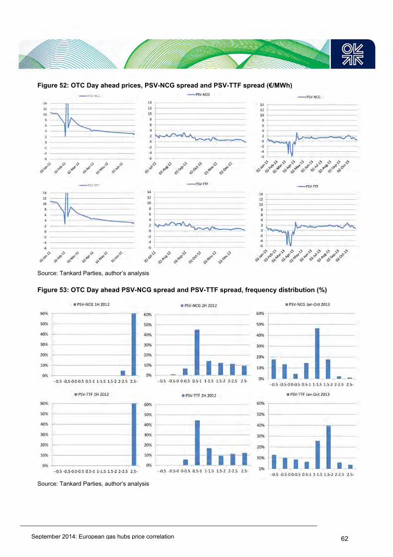
September 2014: European gas hubs price correlation
62
Figure 52: OTC Day ahead prices, PSV-NCG spread and PSV-TTF spread (€/MWh)
Source: Tankard Parties, author’s analysis Figure 53: OTC Day ahead PSV-NCG spread and PSV-TTF spread, frequency distribution (%)
Source: Tankard Parties, author’s analysis

September 2014: European gas hubs price correlation
63
Scatterplots confirm a loose relationship between NCG/TTF and PSV in 1H2012 (also due to the low number of trades for PSV), the abrupt decline in NCG/TTF-PSV spread in mid-September 2012 and a weaker linear relation in the first 10 months of 2013. Figure 54: OTC Day ahead prices, PSV-NCG scatterplot (€/MWh)
Note: red circle indicates days in March 2013 when PSV day ahead prices were below NCG prices Source: Tankard Parties, author’s analysis Figure 55: OTC Day ahead prices, PSV-TTF scatterplot (€/MWh)
Note: red circle indicates days in March 2013 when PSV day ahead prices were below TTF prices Source: Tankard Parties, author’s analysis
Following our methodology, we looked for some evidence for physical pipeline congestion in order to test whether this decline in correlation over 2013 may be explained by PSV and the other Western European Hubs being physically disconnected.
PSV is linked to NCG through the Transitgas pipeline141
. The Transitgas pipeline crosses Switzerland from Wallbach at the German border, where it joins the pipeline system owned by Trans Europa Naturgas Pipeline (TENP), to Passo Gries at the Italian border where it joins the Italian network. TENP runs across the German territory from Bocholtz, at the Dutch border, to the Swiss border, close to Wallbach.
141 Note that PSV is also linked to PEGN as a branch of the Transitgas connects Oltingue on the France-Switzerland border, to Lostorf an interconnection point with the line coming from Wallbach.
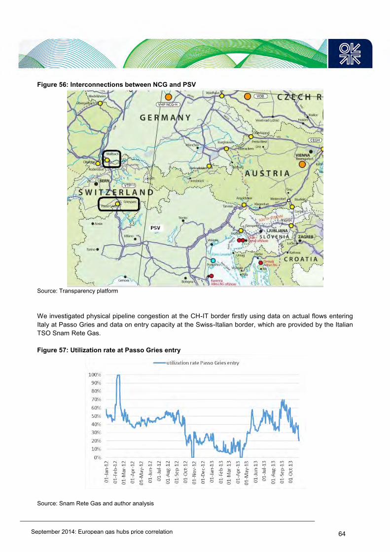
September 2014: European gas hubs price correlation
64
Figure 56: Interconnections between NCG and PSV
Source: Transparency platform We investigated physical pipeline congestion at the CH-IT border firstly using data on actual flows entering Italy at Passo Gries and data on entry capacity at the Swiss-Italian border, which are provided by the Italian TSO Snam Rete Gas. Figure 57: Utilization rate at Passo Gries entry
Source: Snam Rete Gas and author analysis

September 2014: European gas hubs price correlation
65
Over the considered period, Passo Gries interconnection was running at full capacity only few days during the February 2012 crisis, when the OTC day ahead PSV exceeded 50 €/MWh and gained an extraordinary premium to other NWE hubs, making arbitrage extremely profitable. In 2013, apart from a flow interruption from 10 April to 16 April, utilization rate was never critical, ranging from 10% to 70%. The pattern in the utilization rate shows a clear relationship between the amount of imports to Italy and the PSV premium over NCG/TTF: in those periods when the spread is lower imports are less, while gas flows to PSV increase as the premium widens. This is apparent by looking at the reduction in utilization rate in mid-September when the PSV-NCG/TTF spread almost halved. It is widely recognised that spot volumes originating from North West Europe flow through Passo Gries to Italy142. Market players report that every time the spread between TTF and PSV exceeds 1.5 €/MWh, that is roughly the transportation cost from TTF to PSV, there is an increase in spot volumes imported through Passo Gries143. Excluding those few days in the January-October 2013 period when physical congestion (as defined according to our methodology) occurred at Passo Gries, the NCG-PSV correlation did not improve, so does not provide an explanation for the observed de-linkage. Alternative explanations may be found in:
1) the existence of physical/contractual congestion before gas enters Italy and in particular at Wallbach IP. In this regard, ACER reported some contractual congestion at the NCG exit at Wallbach IP144.
2) If 1) does not apply, then the decline in correlation may signal non-efficient market prices or prices not being entirely the result of market forces. In this regard, market players still recognize that the PSV is not liquid (few traders influence the price by timely execution of their trading decisions) and Italy is still an “isolated market”, with no possibility for gas to flow out from the country towards the North145.
Unfortunately we could not test hypothesis 1) due to lack of consistent data. In fact there is no single source for physical flows and capacity data at Wallbach: as the TENP-Transitgas was a transit pipe built in joint venture by several European energy incumbents, as many others in Europe, it is now run by a joint venture between two TSOs, OGE and Fluxys TENP, formerly ENI Deutschland GmbH. Every TSO markets its own capacity share and publishes data on the technical capacity only in its website, but OGE is the only one which publishes total physical flow it on its website. Our results highlight also the fact that PSV and CEGH began to move more closely in 2013. Some factors may have contributed to this:
a better allocation of transport capacity rights between the two markets, in fact : o No congestion between Italy and Austria (Tarvisio-Arnoldstein IP) is occurring, as noted
by ACER146. o There was a release of capacity on the TAG pipeline, allowing more players to trade
between the two hubs.147 o Since October 2013, a day ahead use it or lose it mechanism (UIOLI) is in place at the
Tarvisio-Arnoldstein IP therefore more capacity to flow gas is potentially available.148
142 http://img.en25.com/Web/ICIS/gas-20130130.pdf?cmpid=EMC%7cCHEM%7cCHLEG-2013-01-30-Free-Content_Gas_email1_P1%7c&sfid=701200000008rMp. 143 See for instance: Platts, International Gas Report, Issue 751, 16 June 2014, P.9. 144 ACER (2014) P.19,47,52. 145 For a detailed analysis of the Italian market see Honorè (2013) and for discussion about PSV maturity see Heather (2012). 146 ACER (2014), P.14, Figure 3 147 http://www.icis.com/resources/news/2012/09/07/9593924/italy-s-eni-ups-natural-gas-transport-capacity-offer-to-head-off-antitrust-inquiry/. Official document here: http://www.agcm.it/trasp-statistiche/doc_download/3287-a440chiusura.html

September 2014: European gas hubs price correlation
66
Many participants in CEGH are Italian gas companies149 who may source gas in Austria and import it to Italy. Even if these companies move small volumes compared to Russian long term contract flows, this means that some arbitrage may take place.
In 2013 there was a change in the Italian gas mix: most flows came from Austria (Russian gas), gas originating from NW Europe was less important150 .
Over 2012 and 2013 the price of LTC to Italy was revised and aligned to European hub prices.151
7.7 NBP As mentioned above, the NBP correlation with ZEE (as well as TTF, NCG, GSL, PEGN) significantly declined in 2013 compared to 2012 (from almost 100% to about 90%). The decline in NBP-ZEE was there, although less marked (from almost 100% to about 95%). On the contrary, our scores show that in 2012 NBP was definitely well correlated to the TTF group. On this point ACER commented that in 2012 TTF and NBP price spreads were significantly in line, mainly reflecting GB-NL transmission costs and currency bets and hedges between sterling and the euro152. Figure 58 focuses on de-linkages occurring in the 2H 2012- 2013 period. Figure 58: OTC DA prices at NBP, ZEE, TTF, NCG (€/MWh)
Source: Tankard Parties, author’s analysis
148 AEEG Resolution 411/2013/R/gas, available at: http://www.autorita.energia.it/it/docs/13/411-13.htm 149 http://www.cegh.at/members 150 SnamRete Gas data on flows, see Appendix II for details. 151 Honorè (2013) P.37-42. 152 ACER (2013), P.187.

September 2014: European gas hubs price correlation
67
In winter 2012/13 NBP prices escalated above West Europe hub prices following a reduction in supply (a fall in Norwegian imports due to outages at Ormen Lange and Troll fields, plus erratic LNG flows153) combined with an early cold winter and low utilization of import capacity to GB due to owners of storage gas on the Continent feeling reluctant to withdraw gas so early in the season154. In March 2013, NBP prices increased, triggered by the cold snap, low storage levels, limited LNG imports and, again, a temporary lack of interconnecting capacity, due to outages at a main entry point: Interconnector was down stopping imports from Belgium to UK155. In the May-June period the Interconnector was closed down for maintenance and the prices reacted to this. These facts suggest that a reduction in ZEE-NBP correlation is strongly related to a lack of a physical linkage between the two markets preventing price arbitrage. In particular, based on the assumption that the NBP day-ahead prices respond closely to market fundamentals156, we expected the decrease in NBP correlation to occur during IUK maintenance or when there is scarcity of available spare transport capacity between the two markets. Thus we hypothesise that correlation between ZEE and NBP is generally lower when IUK is shut down for maintenance or when is near to its full capacity. During the 2012/13 winter, GB imported constantly from the Continent and ZEE was on average less expensive than NBP. During the cold snap of March 2013 IUK utilization was near to full capacity (Figure 59). In June 2013 a 13 day maintenance took place preventing the flow of gas between GB and Belgium. The spread between ZEE and NBP, connected directly by the IUK, clearly spiked in March 2013 (when NBP was dearer than ZEE) and during the summer shutdown the NBP was at significant discount to ZEE.
Figure 59: Utilization rate of Interconnector and ZEE-NBP OTC DA price spread (% and €/MWh)
Source: Interconnector, Tankard Parties, author’s analysis
153 CRE Report Q4, Platts Gas Monthly, November 2012. 154 Platts, European Gas Daily, Volume 17 / Issue 214 / November, 5 2012. 155 Platts, Gas Monthly, March 2013. 156 NBP day-ahead contract is widely considered to closely respond to demand and supply forces, as noticed for instance in ACER (2013), P. 186.
-6
-5
-4
-3
-2
-1
0
1
2
3
4
5
-120%-100%
-80%-60%-40%-20%
0%20%40%60%80%
100%120%
IUK flows as a % of full capacity zee-nbp

September 2014: European gas hubs price correlation
68
The availability of spare transport capacity (utilization rate) appears to affect the relationship between ZEE and NBP, as it influences the spread size and direction. As expected, the 2013 correlation between ZEE and NBP improved when excluding those days when IUK was shut down for maintenance or when was near to its full capacity (Figure 60). Figure 60: NBP-ZEE Pearson correlation coefficient over different time periods (%)
Source: Interconnector, Tankard Parties, author’s analysis
8. Volatility Results
8.1 Common trends in price volatility In Figure 61 annual return volatility over the years 2007 to 2013 is compared to the average yearly price level. In general, since 2009 there was a decline in historical yearly volatility levels based on day-ahead price, as opposed to a positive trend in average day ahead prices. 2007 and 2009 generally appear the most volatile years. Although they are similar in terms of volatility level, in 2007 prices were on the rise, while in 2009 the volatility is produced by the rapid fall in prices (at that time prices were falling after the crisis as the market presumably did not know where the 'floor' was). Year 2012 was in general slightly more volatile than 2011, although significantly less volatile than 2008-2010. 2013 (up to October) was the lowest in terms of yearly return volatility for all the hubs but for NBP and the French PEGs. Not only in most recent data the price returns fluctuated over a narrower range of outcomes than in the past, therefore being more ‘predictable’, but also on average these outcomes were lower than in the past: the absolute day-on-day amplitude of price change (MAD) decreased, especially for North West Continental hubs (Figure 62). In fact, the average absolute daily change in price, a measure for “price velocity”, indicates that on average the widest change in prices, above 0.8 €/MWh from one day to the next, occurred at NBP and ZEE in 2008 (CEGH 2008 value is not representative due to a low number of corresponding trades in our sample). In
93%
94%
95%
96%
97%
98%
99%
100%
1H 212 2H 2012 2013 Jan Oct 2013 no Junemaintenance
2013 no Junemaintenance+no March full
capacity
NBP-ZEE
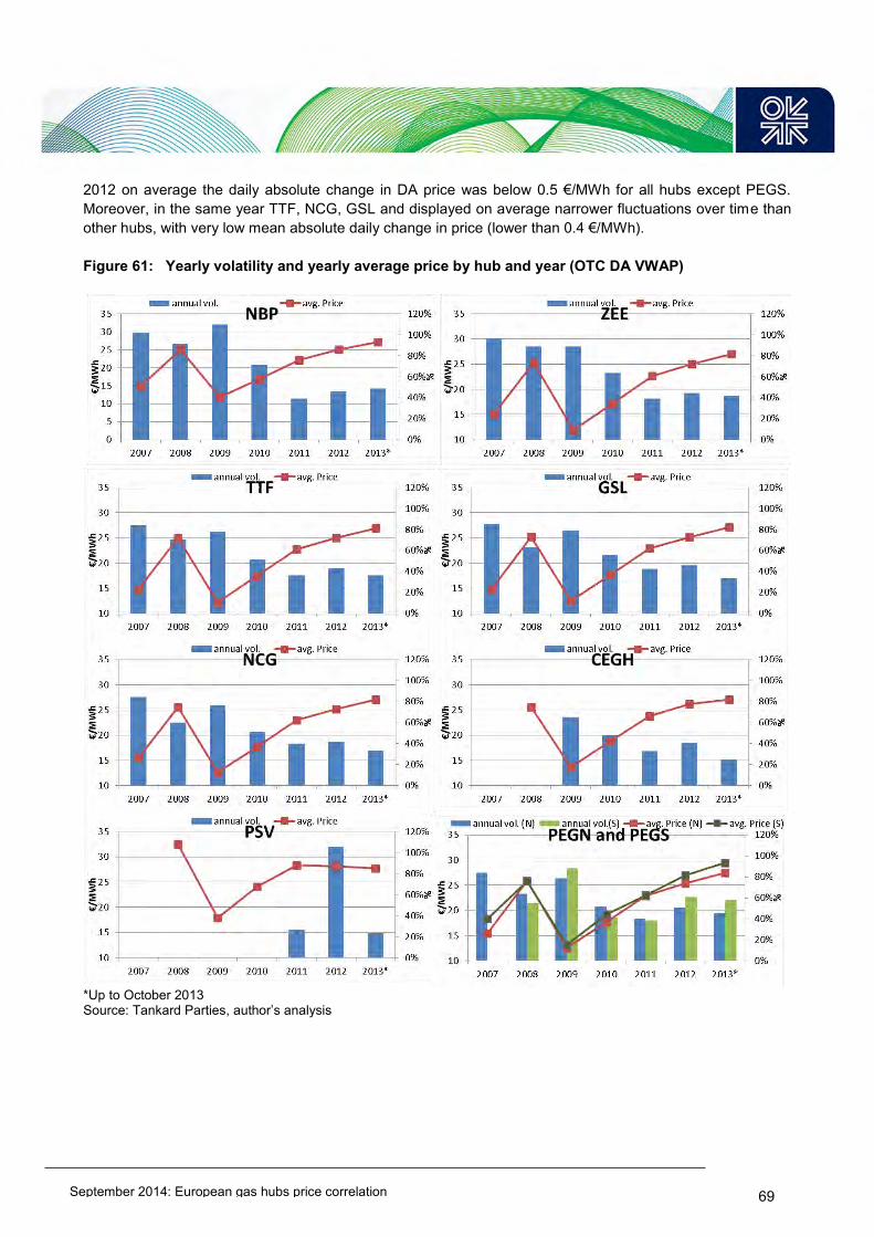
September 2014: European gas hubs price correlation
69
2012 on average the daily absolute change in DA price was below 0.5 €/MWh for all hubs except PEGS. Moreover, in the same year TTF, NCG, GSL and displayed on average narrower fluctuations over time than other hubs, with very low mean absolute daily change in price (lower than 0.4 €/MWh). Figure 61: Yearly volatility and yearly average price by hub and year (OTC DA VWAP)
*Up to October 2013 Source: Tankard Parties, author’s analysis

September 2014: European gas hubs price correlation
70
Figure 62: Annual mean absolute deviation (MAD) by hub
* January-October Source: Tankard Parties, author’s analysis In the most recent data the average absolute daily price change fell even further, achieving record low levels (about 0.3 €/MWh or even less), except for the two sterling quoted hubs and the French hubs. Summing up, the general trend in recent years has been towards lower volatility, although day ahead volatility rebounded in 2012-2013 on the French and British hubs. In very general terms, it might be said that the European and particularly the UK market situation has markedly changed since the mid 2000s. As UK domestic production declined, the North West European market was becoming perceptively ’tight’ with regard to supply, with events such as the Rough outage in the 2005/6 winter creating substantial price escalation. The onset of higher Norwegian imports and LNG provided new supply but also required market participants to include many more variables, including quite possibly the late realisation that Norway (and later the Netherlands) would ‘profile’ their supply to the UK with a winter peak. The lower volatility and the relative higher stability of prices may be explained by the fact that the European gas market moved from a 'tight' situation to the post-2008 phase featuring stagnant demand and a confidence by market players that supply (including storage inventory) in normal times was more than adequate to meet demand. After the crisis there was a surplus of flexibility tools (LNG terminals, pipeline swing, storage) compared to a stagnant outlook for consumption. Such a trend of falling volatility might have been expected to end due to the higher reliance of Europe on Russian supplies in 2014 and 2015 as LNG volumes continue to be diverted to Asia prior to new LNG projects starting up in Australia and Papua New Guinea. However a mild winter in Europe and a mild winter and spring in Asia appears to have created a market in 1H 2014 which is very long in supply relative to demand and high storage inventories in Europe and limited demand for spot LNG in Asia. Paradoxically, although background volatility in the most recent data was indeed subdued across all the hubs compared to the 2007-2010 period, it appears that very extreme spikes have become more frequent than in the past. In other words, prices normally fluctuate less than in the past, but when a shock did occur, the change in price was rather exceptional compared to the rest of the year.
0.0
0.1
0.2
0.3
0.4
0.5
0.6
0.7
0.8
0.9
1.0
NBP ZEE TTF GSL NCG CEGH PSV PEGN PEGS
€/M
Wh
2007 2008 2009 2010 2011 2012 2013*

September 2014: European gas hubs price correlation
71
In fact, the maximum absolute daily change in price, contrary to the MAD, did not reduce over years, but rather showed higher levels in 2012 and 2013 than in previous years (Figure 63). Figure 63: Maximum annual absolute day-on-day change by hub
* January-October Source: Tankard Parties, author’s analysis Additionally, the percentage of trading days when we observe a price spike, defined as a day when the price rises or falls by more than a given threshold157 with respect to the day before, became more frequent (Figure 64). In fact, while from 2007 to 2010 we observe virtually no price spikes, they become common to all hubs in 2012 and to all hubs but for the NBP in 2013. Figure 64: Percentage of trading days when a price spike occurs (%)
* January-October No bar means zero % Source: Tankard Parties, author’s analysis
157 This threshold is defined as twice the yearly standard deviation of prices.
0
1
2
3
4
5
6
7
8
9
10
NBP ZEE TTF GSL NCG CEGH PSV PEGN PEGS
2007 2008 2009 2010 2011 2012 2013*

September 2014: European gas hubs price correlation
72
Note that the NBP is not counted as having a price spike in early 2013, despite the peak in March 2013 (Figure 7). This is explained by the fact on this occasion the daily change in NBP price was indeed larger than in the previous days, but still lower than twice the NBP standard deviation in January-October 2013, which was the highest among the considered hubs.
8.2 Geographical differences in price volatility When we compare the hubs in terms of volatility, it turns out that from 2007 to 2010, the NBP was the most volatile, followed by ZEE; however, in 2011158 the difference in terms of volatility between NBP and the other Continental hubs essentially disappears: volatility is relatively low and similar across European hubs (Figure 65). In 2012 hubs have very similar levels of volatility but for PSV, whose volatility increases significantly (mostly during the February 2012 crisis), PEGS and, to a lesser extent, PEGN. In the January-October 2013 period the differences in terms of volatility between the two sterling quoted hubs and TTF-NCG-GSL enlarge: while the former show yearly volatility scores above 40%, the latter range between 33% and 36%. In 2013 PSV and CEGH volatility was extremely low (<30%), while the French hubs featured the most volatile day ahead prices. The higher level of volatility recorded in the South of France may be linked to PEGS being more dependent on supply coming from regasification terminals in a period of tight LNG market. In 2012 and 2013 lower LNG imports created tensions in areas of Europe which are very dependent on these cargoes and are relatively little interconnected with other European hubs, such as PEGS and Spain159. This though could be temporary. If we move again into a period of LNG supply plenty in the future then volatility at PEGS may decrease.
158 Note that 2010 and 2011 were the years of peak European LNG imports, distributed in North and Southern Europe. This supply availability may have influenced volatility levels. 159 Due to the lack of day-ahead prices for the Spanish market in our data we did not analyse volatility in this market.
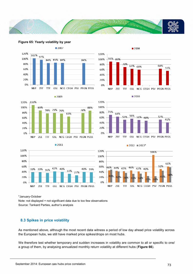
September 2014: European gas hubs price correlation
73
Figure 65: Yearly volatility by year
*January-October Note: not displayed = not significant data due to too few observations Source: Tankard Parties, author’s analysis
8.3 Spikes in price volatility As mentioned above, although the most recent data witness a period of low day ahead price volatility across the European hubs, we still have marked price spikes/drops on most hubs.
We therefore test whether temporary and sudden increases in volatility are common to all or specific to one/ a group of them, by analysing annualized monthly return volatility at different hubs (Figure 66).

September 2014: European gas hubs price correlation
74
Figure 66: Annualized monthly return volatility by hub
Source: Tankard Parties, author’s analysis The chart confirms that since 2010 day ahead volatility declines. Most of the time in 2010 NBP volatility was below 100%, and since 2011 NBP volatility has been below 50%. However, against a background of declining volatility starting from 2010, some isolated spikes stand out. Most of them are common to all the hubs: day ahead price volatility increased dramatically at all the considered markets in February 2012 and in March 2013160. As expected, macro supply/demand factors explain these periods of exceptionally volatility which are shared by all the hubs: the February 2012 crisis161, featuring peak consumption and lack of sufficient Russian supply, and in March 2013 a cold snap combined with low storage levels in Northern Europe. Hubs reacted quite differently to these shocks though (Figure 67). Figure 67: Annualized monthly return volatility in selected months (%)
Source: Tankard Parties, author’s analysis
160 Note that we found no clear relationship between volatility and traded volumes. However at TTF there were more deals in February 2012 and in March 2013 compared to the previous month. 161 Henderson and Heather (2012).
0%
50%
100%
150%
200%
250%
Jan
-07
Ap
r-0
7
Jul-
07
Oct
-07
Jan
-08
Ap
r-0
8
Jul-
08
Oct
-08
Jan
-09
Ap
r-0
9
Jul-
09
Oct
-09
Jan
-10
Ap
r-1
0
Jul-
10
Oct
-10
Jan
-11
Ap
r-1
1
Jul-
11
Oct
-11
Jan
-12
Ap
r-1
2
Jul-
12
Oct
-12
Jan
-13
Ap
r-1
3
Jul-
13
Oct
-13
TTF NBP ZEE GSL NCG CEGH PSV PEGN PEGS
0%
20%
40%
60%
80%
100%
120%
140%
160%
180%
200%
NBP ZEE TTF GSL NCG CEGH PSV PEGN PEGS
Feb 2012 Mar 2013
758%

September 2014: European gas hubs price correlation
75
PSV recorded an extremely high volatility during the February 2012 crisis162, followed by PEGN, PEGS and GSL. Higher volatility at some hubs, and therefore higher price spikes, may be explained by constraints to the free flow of gas from the lower priced markets to the higher priced ones, as is the case with France. During the cold spell import capacity available at Obergailbach and Taisnières H (input capacities to France from Germany and Belgium, respectively) had not been fully utilised, despite the high price differential between the PEGN and neighbouring hubs163. More specifically, the French Energy Regulator CRE noted that 20% of the subscribed entry capacities went unused164. Based on this evidence, the CRE investigated the behaviour of the three main players active on the French wholesale market, who did not fully use their subscribed import capacities at the entry points during the period when the price spikes occurred. The parties mentioned some economic and technical constraints to gas inflows to France, including, among others: the decision by the Italian Government to force the maximization of imports of gas to Italy165 boosting exports from France via Oltingue; and non-availability of firm entry capacities into France as these capacities could be interrupted upon the exit side of the German network166. In the cold early spring of 2013 the UK was more impacted: in a context of low UK storage inventories and concerns over supply due to outages at Norwegian production fields, NBP day ahead prices had to rise substantially and rapidly to encourage pipe imports from the Continent, eventually record IUK flows from the Continent to the UK led to pipeline congestion and the de-linkage discussed in Chapter 7.6. In contrast, South East Europe hubs (PSV, CEGH) were less affected as they were better equipped with storage reserves, which it was not possible to flow towards higher priced markets possibly due to the above discussed barriers to arbitrage flows (Chapter 7.4 and 7.5). Spikes in volatility which are specific to some hubs are closely related to the same factors driving de-linkages:
Starting from 2H 2012 the PEGS volatility pattern diverged from that of other hubs due to the already discussed supply restrictions (Chapter 7.3)
In mid June the sudden drop in NBP prices was due to the outage of IUK which trapped potential gas exports resulting in a gas glut in UK (Chapter 7.6)
162 The exceptional volatility spike for PSV in February 2012 is due to one day priced at 65 (the 8th of Feb 2012) followed by a day (9th of February) with price down at 33.5 €/MWh. On the 8th of February the within day product at PSV was traded at 72 €/MWh. 163 CRE deliberation 26 June 2012, P.2, available at: https://www.google.it/?gfe_rd=cr&ei=TfbIU_TBJMed_waikoDICA&gws_rd=ssl#q=CRE+26+June+2012+deliberation 164 ditto 165 Italian Ministry for Industry communication dated 6 February 2012, http://www.sviluppoeconomico.gov.it/index.php?option=com_content&view=article&viewType=1&idarea1=593&idarea2=0&idarea3=0&idarea4=0&andor=AND§ionid=0&andorcat=AND&partebassaType=0&idareaCalendario1=0&MvediT=1&showMenu=1&showCat=1&showArchiveNewsBotton=0&idmenu=2263&id=2022357 166 CRE deliberation 26 June 2012, P.3, available at: https://www.google.it/?gfe_rd=cr&ei=TfbIU_TBJMed_waikoDICA&gws_rd=ssl#q=CRE+26+June+2012+deliberation
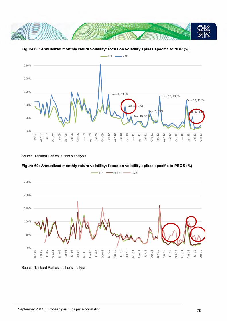
September 2014: European gas hubs price correlation
76
Figure 68: Annualized monthly return volatility: focus on volatility spikes specific to NBP (%)
Source: Tankard Parties, author’s analysis Figure 69: Annualized monthly return volatility: focus on volatility spikes specific to PEGS (%)
Source: Tankard Parties, author’s analysis
Jan-10, 141%
Sep-10, 97%
Dec-10, 58%
Sep-11, 78%
Feb-12, 135%
Mar-13, 119%
Jun-13, 55%
0%
50%
100%
150%
200%
250%
Jan
-07
Ap
r-0
7
Jul-
07
Oct
-07
Jan
-08
Ap
r-0
8
Jul-
08
Oct
-08
Jan
-09
Ap
r-0
9
Jul-
09
Oct
-09
Jan
-10
Ap
r-1
0
Jul-
10
Oct
-10
Jan
-11
Ap
r-1
1
Jul-
11
Oct
-11
Jan
-12
Ap
r-1
2
Jul-
12
Oct
-12
Jan
-13
Ap
r-1
3
Jul-
13
Oct
-13
TTF NBP
0%
50%
100%
150%
200%
250%
Jan
-07
Ap
r-0
7
Jul-
07
Oct
-07
Jan
-08
Ap
r-0
8
Jul-
08
Oct
-08
Jan
-09
Ap
r-0
9
Jul-
09
Oct
-09
Jan
-10
Ap
r-1
0
Jul-
10
Oct
-10
Jan
-11
Ap
r-1
1
Jul-
11
Oct
-11
Jan
-12
Ap
r-1
2
Jul-
12
Oct
-12
Jan
-13
Ap
r-1
3
Jul-
13
Oct
-13
TTF PEGN PEGS
September 2014: European gas hubs price correlation
77
9. Conclusions Our October 2013 paper ’European Gas Hubs: How Strong is Price Correlation?’, suggested that integration of main European gas hubs appeared to have been more or less accomplished and supported the argument that prices at these hubs are the result of demand and supply forces. Hubs in the early stage of development, such as PSV and CEGH, in fact, were becoming more aligned over the time period analysed and it was therefore expected that, with more recent data becoming available, correlation scores would improve. New evidence for 2H 2012 and January to October 2013 167 unexpectedly showed a drop in global correlation, casting some doubts on whether the integration of the main European gas wholesale markets was in fact in place and that all hub price signals could be viewed as reliable. Correlation pair-wise coefficients showed periodical dis-alignments of some hubs and some market segmentation (i.e. a subgroup of hubs which feature closely parallel price movements without being in line with those of the other hubs). In particular, there is a group of geographically proximate hubs that shows very good cross correlations: TTF, German hubs and ZEE. When focusing on this region, we see no decline in correlation from 2012 to 2013 and the correlation remains almost perfect. Correlation against this “core group” decreases however for:
PEGS in 2H 2012, the correlation improves in 2013 but not back to the levels achieved in the beginning of 2012
PEGN, slightly in 2013 CEGH in 2H 2012 and, to a greater extent, in the summer of 2013. PSV, whose correlation with TTF in 2013 is down again at 1H 2012 levels NBP in 2013.
Moreover, the correlation between the Northern and Southern French hubs strengthens in 2013, and more interestingly, PSV-CEGH correlation increases in 2H 2012 and becomes strong in 2013. Returns volatility analysis also detects, even in a context of broadly common volatility patterns across hubs, some spikes in volatility which are specific to some hubs, which are closely related to the same factors driving de-linkages. Is this evidence of a slowing down in the process of wholesale market integration? De-linkages “per se” do not represent hard evidence of a lack of integration and market pricing. Periods of extraordinary low correlation would not be an issue if they could be explained by a combination of local demand/supply shocks and identifiable temporary physical events preventing gas to flow from one hub to the other, such as planned maintenance. We argue that if there is a temporary shock to fundamentals in a market at the same time as physical disconnection and prices consequently delink, then this supports the thesis that prices are the result of supply/demand forces. However, some issues are raised when either the physical congestion is long-lasting or when the driving force behind de-linkages cannot be identified in shutdowns of the connecting infrastructure.
167 This research is supported by data updates on an annual basis.
September 2014: European gas hubs price correlation
78
In the former situation, there may be an infrastructure problem that needs to be addressed and possibly has not been undertaken due to high investment costs. If utilization rates were always near to 1, this may indicate some un-met need for investment in incremental capacity. In this case, price integration is not observed simply because the markets are not interconnected. The problem may also be due to non-physical barriers to cross-border trade. Such barriers are market imperfections that influence players’ behaviours leading to suboptimal use of cross-border interconnection capacities which in turn prevents market players responding effectively to price differentials and eventually restoring good price correlation after a supply/demand shock. Non-physical barriers include: * inconsistency in the adjacent market systems (for instance definition of interruptible and firm capacities not harmonised either side of the borders); * market power abuse (for instance capacity hoarding practices); * too high transaction costs or information asymmetry (for instance lack of transparency in the capacity allocation procedures, including possibly insufficient disclosure to market players regarding available capacity). When this is the case, a revision of commercial arrangements and/or regulatory provisions to use transport capacity is required to alleviate the bottleneck. Among the identified de-linkages those affecting NBP and PEGN proved to be the consequence of identifiable temporary lack of physical connections and so do not indicate a slowdown in the integration process. PEGS mis-alignment is instead the result of sub-optimal infrastructural physical capacity, suggesting that here pipeline capacity needs to be expanded to achieve integration, but perhaps there is no incentive or framework to do so. As mentioned previously, the need of further investment in the network has been identified and addressed. Lack of reliable and consistent data on gas flows prevent us firmly concluding that non-physical barriers to integration and, in particular issues with capacity accessibility, were the driving force behind CEGH and PSV de-linkages. However, some evidence points in this direction. This being the case, we should consider whether further policy measures are needed to achieve the declared EU goal of gas wholesale market integration168. In this debate, it is key to decide first whether a perfect correlation is needed to achieve the EU objectives and whether other metrics may be more adequate or desirable169. We argue that if all de-linkages may be explained by temporal physical constraints, ensuring constant alignment may come at too high a cost for society in terms of transport facilities. However, price de-linkages that persist due to market inefficiencies represent a poor use of assets for which investment has been made in the past, with consumers suffering a financial burden for such inefficiencies. We suspect this may be case with the CEGH and PSV de-linkages. Therefore, if good price correlation is desirable, we pose the question as to whether the current EU initiatives for the Single Gas Market will solve these problems, by creating adequate incentives to expand interconnecting capacity and/or by solving contractual congestion problems and other non-physical barriers to trade.
168 We do not discuss here he advantages of integration, as this is beyond the scope of the paper. 169 As extensively discussed in Chapter 2.

September 2014: European gas hubs price correlation
79
We argue that the precondition to answering this question is having access to reliable evidence in terms of gas flows and interconnecting capacity at IPs. Some effort seems to be needed in this direction. Only reliable data and transparency allows the correct identification of these problems and consequently what is required to address them. It appears quite probable (but not proven) that the changing scale and geographic pattern of LNG imports into Europe over the past four years and (possibly) the start-up of Nord Stream are triggers or at least mitigating factors in creating/exposing such bottlenecks and their expression in the form of price de-linkages. It is quite possible therefore that a return to an equally well LNG-supplied Europe in the future could alleviate such bottlenecks, at least for a while. However, debottlenecking intervention and remedy perhaps should be viewed as a necessary ongoing cost to allowing arbitrage to function in an inevitably evolving supply pattern situation. The EU Regulators and system operators may still have work to do to eliminate barriers to cross-border trade, in particular the non-physical ones.
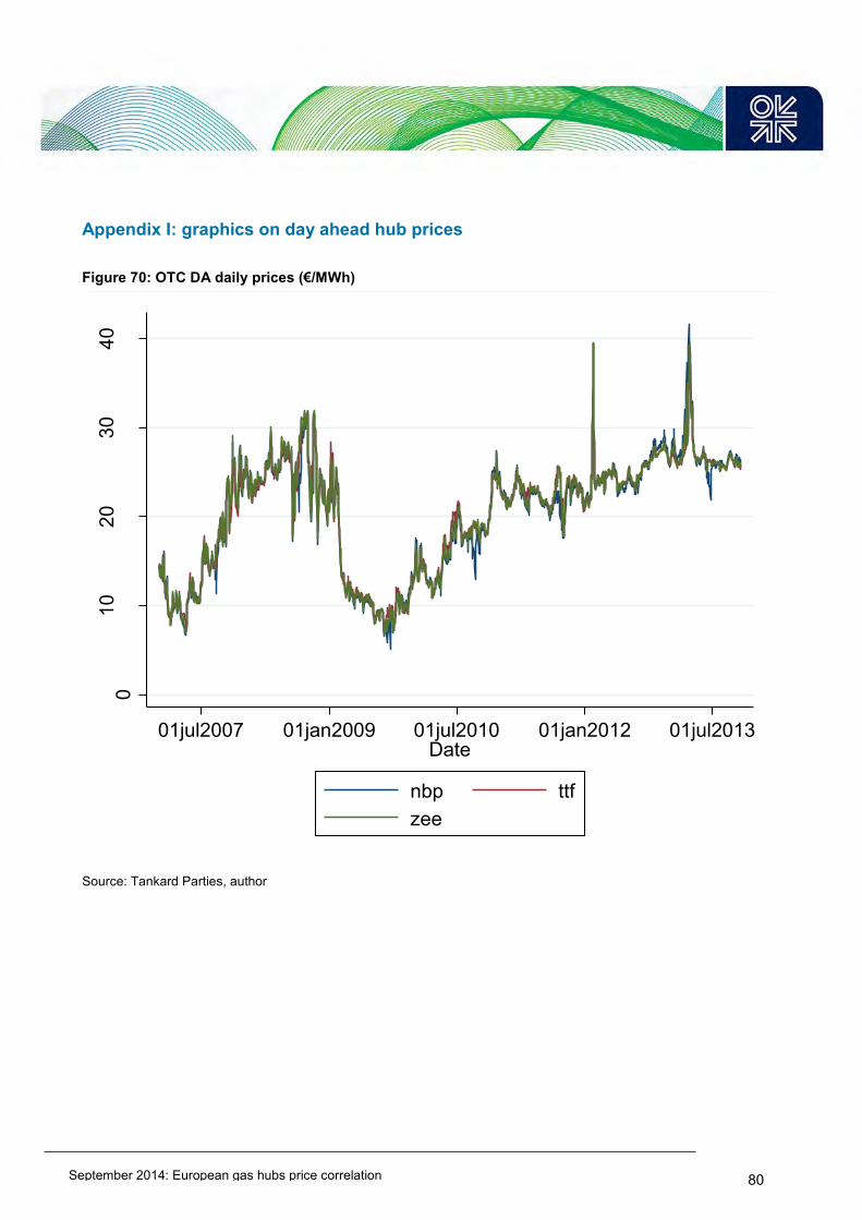
September 2014: European gas hubs price correlation
80
Appendix I: graphics on day ahead hub prices Figure 70: OTC DA daily prices (€/MWh)
Source: Tankard Parties, author
010
2030
40
01jul2007 01jan2009 01jul2010 01jan2012 01jul2013Date
nbp ttfzee

September 2014: European gas hubs price correlation
81
Figure 71: OTC DA daily prices (€/MWh)
Source: Tankard Parties, author
1020
3040
01jul2007 01jan2009 01jul2010 01jan2012 01jul2013Date
ttf gslncg

September 2014: European gas hubs price correlation
82
Figure 72: OTC DA daily prices (€/MWh)
Source: Tankard Parties, author
1020
3040
50
01jul2007 01jan2009 01jul2010 01jan2012 01jul2013Date
ttf pegnpegs

September 2014: European gas hubs price correlation
83
Figure 73: OTC DA daily prices (€/MWh)
Source: Tankard Parties, author
020
4060
01jul2007 01jan2009 01jul2010 01jan2012 01jul2013Date
ttf ceghpsv
September 2014: European gas hubs price correlation
84
Appendix II: data creation: exchange price, flow and capacity data Data creation Raw data from brokers (specifically the Tankard Parties) and exchange websites were assembled and sampled to obtain streams of daily historical price data and related total daily traded volumes for the selected traded contracts, building up a database of prices and volumes prevailing at the main European gas trading hubs. The data set has separate daily price series for exchange traded and OTC traded products, to check for any difference when comparing broadly equivalent contracts. Note that exchange cleared OTC transactions were excluded (so called “given up for clearing” OTC trades or “OTC broker give up”) from OTC trades, as although they are recorded by brokers these trades effectively occurred via exchanges. Computation of daily average prices The daily price was computed as the volume-weighted average of the prices of the transactions occurring in a day. However, this average may be computed averaging over either: (1) prices of trades executed within a restricted time period (the so called “settlement window”) at the end of the trading day (obtaining an End of Day Price also known as Settlement Price) or (2) all the orders executed within the whole trading day (obtaining a Daily Average Price). We chose a Daily Weighted Average Price rather than a Settlement price. It is worth noticing that the latter is usually considered as a price reference by Price Reporting Agencies and settlement prices are published by exchanges (EEX for instance). Traded volume Please note that one trade volume is the daily flow rate volume multiplied by the number of days in the contract. For instance if two parties conclude a Calendar Year 2014 contract and commit to the delivery of a daily lot size of 240 MWh/d , we count the corresponding total traded volume as 240*365 MWh. Selected hubs The market hubs considered correspond to those extensively described in Heather (2012). Before 2009 transactions ascribed to Gaspool (GPL) and NCG correspond to the hubs that were subsequently merged to form GPL and NCG respectively. Points of delivery were grouped into hubs as follows:

September 2014: European gas hubs price correlation
85
Table 7: Delivery points associated with each hub
Source: Author Unit of measurement and conversion factor All price data is in €/MWh and volumes are in MWh. NBP and ZEE prices, originally expressed in pence/therm, were converted to €/MWh assuming a conversion factor of 29.3071 MWh/1000 therms. The recently launched ZTP quotes prices in €/MWh, so prices for ZTP trades were not converted. We converted pence/therm prices into €/MWh prices using the daily average euro/ GB sterling exchange rate as published by OANDA170. The relevant exchange rate is the daily average euro/ GB sterling exchange rate of the day of the trade for all products. Identification of month ahead product As the month ahead contract may not be explicitly identified in the raw data, when necessary the following assumption is made: trading for the month ahead contract ceases on the last business day of the month. Exchange price data The sources are the following. Table 8: Sources for exchange prices used in this study Contract Source PEGN DA Powernext PEGS DA Powernext NCG DA EEX ZEE DA ICE-ENDEX TTF DA ICE-ENDEX CEGH DA CEGH gas exchange Source: Author
TTF DA exchange price From 2 January 2006 to 31 Dec 2011: APX ENDEX (former ICE-ENDEX) TTF All Day Index data (prices quoted in €/MWh, volumes in MWh). The APX TTF All-day Index is a volume-weighted average price of all single day trades on TTF executed between 06:00 CET and 18:00 CET on the day prior to settlement (for example, if the index is to be calculated for 4th May, eligible trades will be those made on 3rd May). If there are no trades on TTF within the time period specified above, a default procedure is employed to generate a default index value, for the day in question. 170 http://www.oanda.com/currency/historical-rates/
NBP TTF CEGH ZEE PSV PEGS GASPOOL NCG
NBP TTF G + 44.4 BAUMGARTEN Zeebrugge Hub PSV PEG NORD_H BEB_VEP-H EGT_VP_MID_H GAS
TTF Hi Cal 51.6 BAUMGARTEN MS 2 ZTP PEG Est BEB_VEP-L EGT_VP_NORTH_H GAS
BAUMGARTEN MS 3 PEG Sud GASPOOL EGT_VP_SOUTH_H GAS
BAUMGARTEN ITAB PEG ouest ONTRAS_VP EGT_VP-H
Baumgarten (TAG) PEG GSO EGT_VP-L
Baumgarten (WAG) PEG-TIGF EGT_VP-MID-H
ITAB (Baumgarten) EGT_VP-NORTH-H
VTP EGT_VP-SOUTH-H
NCG
NCG L
September 2014: European gas hubs price correlation
86
On 16 January 2012 APX-ENDEX ceased publication of the APX TTF All-day Index and replaced it with the APX TTF Day-Ahead Index. From 1 Jan 2012 onwards: ICE-ENDEX TTF Day-Ahead Index (prices quoted in €/MWh, volumes in MWh). The APX TTF Day-Ahead Index is a volume-weighted average price of all orders which are executed on the gas day before the day of delivery and consists of two indices:
1. The APX TTF Next-Day Index for next-day delivery on working days: This index is the volume-weighted average price of all TTF Day contracts which are concluded on Monday through Friday for delivery on the next working day. The APX TTF Day-Ahead Index for Monday is based on the trades concluded on the Friday before.
2. The APX TTF Weekend Index for delivery on Saturday and Sunday: This index is the volume-weighted average price of all TTF Day and TTF Weekend contracts which are concluded on Friday for delivery on Saturday and/or Sunday.
We considered the daily index only when it corresponds to an actual trade (i.e. corresponding total daily volumes are greater than zero). The index refers to a daily average price, rather than to a Closing or End of Day price. We did not use a list of transaction prices (which was not available) but rather a daily average price as computed by the Exchange operator. For the Day-Ahead and Within-Day products, the ICE Report Center offers a 7-day price history, while full price index history is available via the Download Center in xls format. ICE ENDEX website offers free data access, historical data is provided free of charge. We did not consider ICE, EEX, or Powernext quotations for TTF contracts, although they exist.
PEGN and PEGS DA exchange price
These data are based on Powernext exchange data (prices quoted in €/MWh, volumes in MWh) 171 : Powernext Gas Spot Daily Prices (Daily Average Price). The Powernext website provides historical data on all the trades executed each day on Powernext.
NCG DA exchange price These are volume-weighted averages over EEX Gas Spot Market settlement prices172 for contracts “next day 10 MW” and “next day 1 MW”, for delivery at NCG, provided that the delivery day is the day after the trading day. The settlement window is 5-5:15 pm.
ZEE DA exchange price From 1 January 2007 to 30 Sep 2012: APX endex All Day index Zeebrugge Since 1 October 2012: ZTPH Natural Gas day-ahead index. We considered the daily index only when it corresponds to an actual trade (i.e. corresponding total daily volumes are greater than zero). The index refers to a daily average price, rather than to a Closing or End of Day price. We did not use a list of transaction prices (which was not available) but rather a daily average price as computed by the Exchange operator.
171 Powernext data, including the comprehensive record of all the trades concluded on the spot and future market, are free to download on the website http://www.powernext.com/#sk;tp=app;n=market;f=listMarketTable;t=layout/gasSpot;fp=system_name:gasSpot;lang=en_US;m=Market_Data. 172 EEX historical price and volume data are available on a fee basis. EEX publishes every day on its website daily price and volumes for the traded contracts.

September 2014: European gas hubs price correlation
87
For the Day-Ahead and Within-Day products, the ICE Report Center offers a 7-day price history, while full price history is available via the Download Center in xls format. Both websites offer free data access.
CEGH DA exchange price
We considered the daily CEGH Spot Index CEGHIX173. We consider the index only when corresponding total daily volumes are greater than zero. CEGH started publishing CEGHIX index in February 2012. On its website CEGH publishes Gas Exchange Market Data of the last seven days.
Flow data
Obergailbach IP entry to France, Taisnieres H IP entry to France, Taisnieres B IP entry to France:
Physical flows (in kWh 25°C) as published by GRTgaz (http://www.smart.grtgaz.com/en/flux_physiques/PIR) Technical effective capacity (in kWh 25°C) as published by GRTgaz (http://www.smart.grtgaz.com/en/flux_commerciaux/PIR)
Passo Gries IP entry to Italy Daily physical flows (in mcm) as published by Snam Rete Gas (http://www.snamretegas.it/it/servizi/Quantita_gas_trasportato/2_Andamento_dal_2005/?formindex=1&archive_year=2013) Firm technical available capacity (59 mcm/d) as published by Snam Rete Gas (for Gas Year 2012: http://www.snamretegas.it/it/servizi/Anno-termico_2012_2013/Capacita_trasporto/index.html)
Bacton/Zeebrugge IP entry to UK and exit from UK Interconnector pipeline daily physical flows (in kWh) as published by Interconnector (http://www.interconnector.com/operational-data/historical-data/data-downloads/) Technical capacity considered to be: import to UK 69.9 mcm/d, export from UK 54.79 mcm/d
173 See http://www.cegh.at/ceghix for more details.

September 2014: European gas hubs price correlation
88
Glossary Bcm: One billion cubic metres. Box-plot: A box-plot is a way of summarizing a set of data measured on an interval scale. It is often used in exploratory data analysis. It is a type of graph which is used to show the shape of the distribution, its central value, and variability. Box plots have a main rectangular body (the box itself) and lines extending vertically from the box (so called whiskers). The bottom and top of the box are the first and third quartiles, and the band inside the box is the median; the ends of the whiskers represent the upper and lower adjacent values: the largest value smaller or equal to upper quartile + 1.5 IQR (where IQR is the interquartile range, a measure of statistical dispersion, being equal to the difference between the upper and lower quartiles, IQR = Q3 − Q1) and the smallest value greater or equal to the lower quartile - 1.5 IQR. Any points more extreme then the upper and lower adjacent values are represented as dots. The length of the box represents the IQR and helps indicate the degree of dispersion (volatility) in the data: the more stretched the box is, the more variable prices are within the year. The length of the whiskers is another measure of dispersion; while dots identify outliers, i.e. isolated price peaks or troughs that do not fit the general trend. Broker: a party who intermediates and facilitates bilateral contracts to be concluded between a buyer and a seller. CAM: capacity allocation mechanism CEGH: Central Europe Gas Hub CMP: congestion management procedures Coefficient of variation (CV): normalized measure of dispersion of a frequency distribution: the ratio of the standard deviation to the mean. The actual value of the CV is independent of the unit in which the measurement has been taken, so it is a dimensionless number and, for comparison between data sets with different units or widely different means, the coefficient of variation is preferred to the standard deviation. Co-integration analysis: econometric technique developed for the analysis of time series. Contract settlement: resolution of a contract at its expiry. A contract may be settled through physical delivery, by cash settlement or by settling the payment and “giving up the volume” to an exchange that is by tendering the quantity of gas on an exchange platform for whatever price it can be sold for. Correlation: (see Pearson Product-Moment Correlation coefficient) Day ahead (DA) contract/product: contract for the purchase or sale of gas to be delivered the day after the trading date. Delivery/net physical delivery: the moment when a player makes a nomination to the system operator, who in turn uses this input to compute the total volume to be injected/withdrawn into the grid. Nomination is made before gas has to be injected/withdrawn in the grid. In the UK nomination has to be made for gas to be injected/withdrawn into the grid the following day (day d). A player nomination is computed by netting off all the traded volumes relating to the day ahead. Elasticity: the measurement of how responsive a variable is to a change in another. An elastic variable is one which responds more than proportionally to changes in other variables. In contrast, an inelastic variable is one which changes less than proportionally in response to changes in other variables. Entry-exit system a system where gas can be traded independently of its location in the pipeline system, with the possibility for network users to book entry and exit capacity independently, creating gas transport through zones instead of along contractual paths. Exchange trade: anonymous and regulated trade whereby the buyer and the seller of gas have the exchange operator as a central counterparty operating as a clearing house. Financial trade: trade which is settled without the actual delivery of gas but rather through a cash payment, normally of the difference between the agreed price and the outturn spot price. Forward gas contract: contract for the purchase or sale of gas to be delivered on a future agreed date (delivery date).

September 2014: European gas hubs price correlation
89
Gross traded volumes (traded volumes): the total gas amounts that are traded on each hub which are usually a multiple of the physical quantity that is actually delivered on the grid. Traded volumes can exceed consumed physical volumes in a commodity market as quantities can be bought and sold many times prior to delivery. GSL: Gaspool, gas hub based in Germany. GTM (Gas Target Model): conceptual model for the single European gas markets developed by CEER in 2011, it is currently subject to an update. H-gas: High-calorific gas (also called H-gas or high gas) is the highest quality natural gas due to its high methane content (between 87% and 99%). HHV: The higher heating value (HHV: also known as the gross calorific value or gross energy) of a fuel is defined as the amount of heat released by a specified quantity (initially at 25 °C) once it is combusted and the products have returned to a temperature of 25 °C. It thus includes the latent heat of condensation of water in the combustion products. Hub (gas hub): a virtual or physical location within the grid where the exchange of gas volumes takes place. In fact a gas hub is a market for gas, where the commodity is traded on a standardized basis between market participants.In this paper each hub represents a different price area. Inelasticity: (see Elasticity) Interconnection Point: Means a location, whether it is physical or virtual, between two or more EU Member States as well as between two adjacent entry-exit-systems within the same Member State, where the pipeline systems of the two adjacent Member States or entry exit system join. Interconnector (IUK): the bi-directional pipeline allowing the flow of gas from Britain to Belgium and vice versa. Interquartile range (IQR): a measure of statistical dispersion, used also for non parametric data, being equal to the difference between the upper and the lower quartiles: Q3-Q1. It measures volatility in absolute terms. kWh: A unit of energy equivalent to a Kilowatt of power for the duration of one hour. LEBA volume report: regular monthly volume report covering the main gas, power, coal and emission markets, published by LEBA. LEBA volume data are available from January 2011. LEBA: the London Energy Brokers’ Association, is the industry association representing the FSA regulated wholesale market brokers in the over the counter (OTC) and the exchange traded UK and liberalised European energy markets. The major products that they deal in include crude oil and refined petroleum products, gas, electricity and emissions. L-gas: Low-calorific gas (L-gas or low gas) is natural gas with a lower methane content of between 80% and 87%. LTC: long term contract for the sale and purchase of natural gas. MAD: mean absolute deviation, mean of absolute daily change in price in a given period. mcm: One million cubic metres. Month ahead (MA) or front month contract/product: contract for the purchase or sale of gas to be delivered in the month after the trading date. MWh: A unit of energy equivalent to a Megawatt of power for the duration of one hour. NBP: National Balancing Point, gas hub based in Great Britain. NCG: Net Connect Germany, gas hub based in Germany. OTC (over the counter) trades: bilateral non-regulated trade however involving standardized physical and financial deals. Such trades are based on standard agreements defining the point of delivery for gas along with other technical and legal terms. They can be for standard volumes of clip sizes of gas and multiples thereof. Pearson Product-Moment Correlation coefficient (Pearson coefficient, r): statistical metric which measures the strength of the linear relationship (linear correlation) between two data series. The correlation coefficient always takes a value between -1 and 1, with 1 or -1 indicating perfect correlation (all points would lie along a straight line in this case). A positive correlation indicates a positive association between the

September 2014: European gas hubs price correlation
90
variables (increasing values in one variable correspond to increasing values in the other variable), while a negative correlation indicates a negative association between the variables (increasing values in one variable correspond to decreasing values in the other variable). A correlation value close to 0 indicates no association between the variables. PEG: Points d’Echange de Gaz including Peg Nord (Peg North), Peg Sud (Peg South) and Peg TIGF hubs, based in France. Physical trade: trade which is settled at expiry by the actual delivery of gas. Price correlation: when prices move closely in parallel over time. Price de-linkage: period of low correlation. PSV: Punto di Scambio Virtuale, the Italian gas hub. Relative law of one price: in a competitive market the price of a homogeneous good should tend towards uniformity, allowances being made for transportation and other transaction costs. Return: The logarithmic price change or logarithmic return, r, is: r = log (Pt+d /Pt), where Pt is the initial price and Pt+d is the price after one period, for instance after one day. The arithmetic price change or arithmetic return, R, is: R = (Pt+d – Pt)/ Pt. Both the logarithmic return and the arithmetic return measure the price change relative to an initial price, when returns are small these measures are close. Scatter plot: useful summary of a set of bivariate data (two variables), usually drawn before working out a linear correlation coefficient or fitting a regression line. It is a mathematical diagram using Cartesian coordinates plotting one variable against the other. It gives a good visual picture of the relationship between the two variables, and aids the interpretation of the correlation coefficient or regression model. Each unit contributes one point to the scatterplot, on which points are plotted but not joined. The resulting pattern indicates the type and strength of the relationship between the two variables. Significance level: In statistics and probability theory, is the low probability of obtaining at least as extreme results given that the null hypothesis is true Standard deviation: In statistics and probability theory, the standard deviation (SD) (represented by the Greek letter sigma, σ) measures the amount of variation or dispersion from the average. A low standard deviation indicates that the data points tend to be very close to the mean (also called expected value); a high standard deviation indicates that the data points are spread out over a large range of values. Tankard Parties: Tankard is an industry initiative created and developed by ICAP Energy Limited (ICAP), Marex Spectron Group (Marex Spectron) and Tullett Prebon Group Limited (Tullett Prebon). TENP: the gas pipeline that runs across the German territory from Bocholtz, at the Dutch border, to the Swiss border, close to Wallbach, where it joins Transitgas. Transitgas: the gas pipeline that crosses Switzerland from Wallbach at the German border to Passo Gries (Gries Pass) at the Italian border. At Wallbach Transitgas joins the Trans Europa Naturgas Pipeline (TENP), at Passo Gries it joins the Italian network. Transmission System Operator (TSO): the company responsible for the transmission system operation. Some countries have one gas TSO, others have several TSOs. TTF: Title Transfer Facility, gas hub based in the Netherlands, Volatility: see Chapter 4 WAG: bidirectional pipeline running from Oberkappel to Baumgarten, Austria. Oberkappel is the IP located at the extreme of WAG located on the Germany-Austria border, Baumgerten is the IP located at the extreme of WAG located on the Austria-Slovakia border. WAG can be used in a flexible way for arbitrage flows. Through WAG Austria can import gas directly from NCG, in addition, gas coming mostly from Russia can also flow through this pipeline in the opposite direction. WAP: weighted average price ZEE: Zeebrugge, gas hub based in Belgium.

September 2014: European gas hubs price correlation
91
Bibliography ACER (2013): ACER Annual Market Monitoring Report 2013 http://www.acer.europa.eu/Official_documents/Acts_of_the_Agency/Publication/ACER%20Market%20Monitoring%20Report%202013.pdf
ACER (2014): ACER Annual report on congestion at interconnection points in Q4/2013, http://www.acer.europa.eu/Official_documents/Acts_of_the_Agency/Publication/ACER%20Gas%20Contractual%20Congestion%20Report%202014.pdf
Alterman (2012): Alterman, Sofya, Natural Gas Price Volatility in the UK and North America, NG 60, OIES, February 2012. http://www.oxfordenergy.org/2012/02/natural-gas-price-volatility-in-the-uk-and-north-america/ Asche et al. (2010) : Asche, F., Øglend, A., Osmundsen P., and M. Sikveland (2010), Volatility and risk sharing in European gas markets, proceedings, International Association for Energy Economics (IAEE), Vilnius, 26-28 august. Benini et al. (2002): Benini, M.; Marracci, M.; Pelacchi, P.; Venturini, A. Day-ahead market price volatility analysis in deregulated electricity markets. In Proceedings of the IEEE Power Engineering Society Summer Meeting, Chicago, IL, USA, 25 July 2002; Volume 3, pp. 1354–1359. Boisseleau (2004): Boisseleau, F. The role of power exchanges for the creation of a single European electricity market: market design and market regulation, Phd Dissertation Thesis, Université Paris IX Dauphine, France, http://repository.tudelft.nl/view/ir/uuid%3Aadaa3685-ff74-4ad6-b765-752f1a673c4c/ CEER (2011): CEER Vision for a European Gas Target Model. Conclusions Paper, Ref: C11-GWG-82-03, 1 December 2011. Available at http://www.energy-regulators.eu/portal/page/portal/EER_HOME/EER_PUBLICATIONS/CEER_PAPERS/Gas/Tab/C11-GWG-82-03_GTM%20vision_Final.pdf Cont (2005): Cont, Rama, Volatility Clustering in Financial Markets: Empirical Facts and Agent-Based Models. Available at SSRN: http://ssrn.com/abstract=1411462 or http://dx.doi.org/10.2139/ssrn.1411462 CRE (2013a): CRE, Electricity and Gas Market Observatory 1Q 2013 available at: http://www.cre.fr/en/markets/electricity-and-gas-market-observatory CRE (2013b): CRE, Electricity and Gas Market Observatory 2Q 2013 available at: http://www.cre.fr/en/markets/electricity-and-gas-market-observatory CRE (2013c): CRE, Electricity and Gas Market Observatory 3Q 2013 available at: http://www.cre.fr/en/markets/electricity-and-gas-market-observatory
De Jong and Schneider (2009): Cyriel de Jong (KYOS) and Stefan Schneider (EON Energy Trading) “Cointegration between gas and power spot prices” Journal of Energy Markets, Fall 2009
Doane and Spulber (1994): Doane, J. M. and Spulber D. F. (1994). ‘Open access and the evolution of the U.S. spot market for natural gas’ Journal of Law and Economics, Vol. 37, No. 2, pp. 477-517.

September 2014: European gas hubs price correlation
92
E-Control (2012): E-Control, Annual Report 2012, http://www.e-control.at/portal/page/portal/medienbibliothek/publikationen/dokumente/pdfs/e-control-annual-report-2012.pdf
EIA (2007): EIA An analysis of price volatility in Natural Gas Markets, 2007, http://www.eia.gov/dnav/ng/ng_pub_analysis_pri.asp GME (2014): Gestore Mercati Energetici (GME), Annual Report 2013, available at: https://www.mercatoelettrico.org/en/GME/Biblioteca/RapportiAnnuali.aspx Heather (2012): Heather, Patrick, Continental European Gas Hubs: are they fit for purpose?, NG 63, OIES, June 2012. http://www.oxfordenergy.org/2012/06/continental-european-gas-hubs-are-they-fit-for-purpose/ Henderson and Heather (2012): Henderson,J and Heather,P, Oxford Energy Comment “Lessons from the February 2012 European gas “crisis”, April 2012. http://www.oxfordenergy.org/2012/04/lessons-from-the-february-2012-european-gas-%e2%80%9ccrisis%e2%80%9d/ Henning et al (2003): Henning, B., Sloan M. and De Leon, M., Natural Gas and Energy Price Volatility, American Gas Foundation, 2003. http://www.gasfoundation.org/ResearchStudies/volatility.htm Honorè (2013): Honorè, Anouk, The Italian Gas Market - challenges and opportunities, NG76, OIES, June 2013. http://www.oxfordenergy.org/2013/06/the-italian-gas-market-challenges-and-opportunities-2/ Li and Flynn (2004): Li, Y.; Flynn, P.C. Deregulated power prices: Comparison of volatility. Energy Policy 2004, 32, 1591–1601. Lin and Prince (2013): Cynthia Lin and Lea Prince “Gasoline price volatility and the elasticity of demand for gasoline”, Energy Economics, Volume 38, July 2013, Pages 111–117 Petrovich (2013): Petrovich, Beatrice, European gas hubs: how strong is price correlation?, NG79, OIES, October 2013. http://www.oxfordenergy.org/2013/10/european-gas-hubs-how-strong-is-price-correlation-2/ Regnier (2007): Regnier, E. Oil and energy price volatility. Energy Econ. 2007, 29, 405–427. Ruiz et al. (2012): Ruiz at al. A New Approach to Measure Volatility in Energy Markets, Entropy 2012, 14, 74-9 Simonsen (2005): Simonsen, I. Volatility of power markets. Phys. Stat. Mech. Appl. 2005, 335, 10–20. Stigler and Sherwin (1985): Stigler, G. J., and Sherwin, R. A, ‘The Extent of the Market’ Journal of Law and Economics 28, pp. 555-585. Zareipour at al. (2007): Zareipour, H.; Bhattacharya, K.; Canizares, C. Electricity market price volatility: The case of Ontario. Energy Policy 2007, 35, 4739–4748.