EUROPEAN COMMISSION DIRECTORATE … Research Centre/jrc...List of national elements attending the...

EUROPEAN COMMISSION

DIRECTORATE GENERAL JRC

JOINT RESEARCH CENTRE

Institute of Environment and Sustainability

WFD Intercalibration Phase 2: Milestone 6 report

Water category/GIG/BQE/

horizontal activity: Rivers/ Mediterranean GIG/ Macrophytes

Information provided by: Francisca Aguiar

1. Organisation

1.1. Responsibilities

Indicate how the work is organised, indicating the lead country/person and the list of involved

experts of every country:

The Mediterranean GIG met once or twice every year, under the coordination of Maria Teresa

Ferreira. On these annual meetings the progression of the BQE was discussed, either at the BQE

level or collectively. Some independent BQE meetings also took place and other relevant

meetings were attended by the BQE leaders.

The BQE macrophyte working group leader was Francisca Aguiar, Portugal, responsible for the

reception and homogeneization, data analyses, harmonisation and reporting. List of national elements attending the meetings (not necessarily all meetings):

Cyprus: Paraskevi Manolaki (macrophyte expert), Eva Papastergiadou (macrophyte expert),

Gerald Dörflinger, Iakovos Tziortzis

France: Christian Chauvin (macrophyte expert), Martial Férreol, Laurence Blanc, Michael

Cagnant, Nicolas Roset, François Delmas, Juliette Rosebery, Yorik Reyjol

Greece: Paraskevi Manolaki (macrophyte expert), Eva Papastergiadou (macrophyte expert), ,

Stamatis Zogaris, Phoebe Vayanou, Michalis Maroulakis, Ioannis Karavokris

Italy: Maria Rita Minciardi (macrophyte expert), Simone Ciadamidaro, Laura Mancini, Camilla

Puccinelli, Stefania Marcheggiani, Stefania Erba, Andrea Buffagni

Slovenia: Mateja Germ (macrophyte expert), Gorazd Urbanič, Nina Stupnikar, Vesna Petkovska

Spain: Jaume Cambra (macrophyte expert), Jose Luis Moreno (macrophyte expert), Narcis Part,

Sergi Sabater, Elisabet Tormes, Nuno Caiola, Antoni Munné, Ana Lara, Fernando Gurucharri,

Irene Carrasco

Portugal: Maria Teresa Ferreira, Maria João Feio, Salomé Fernandes, Pedro Segurado, Francisca

Aguiar (macrophyte expert), João Ferreira

1.2. Participation

Indicate which countries are participating in your group. Are there any difficulties with the

participation of specific Member States? If yes, please specify:

Seven Member States are participating in the Med GIG macrophytes – Portugal, Spain,

Greece, Cyprus, Italy, France and Slovenia.

The Greek participation is insured voluntarily by the Patras University. The official participation

of Patras University in the macrophytes Med GIG group is under discussion with the Greek

Ministry of Environment.

Malta did not rely to e-mails and contacts.

On 24-05-2011, there was an e-mail contact from the water administration of Bulgaria,

expressing interest to follow our group activities. It was too late to be able to incorporate these

results because it would require time for data collection (environment, pressure, biotic) similar to

the one performed during the first two years of the IC2 exercise. Bulgaria was informed of the

Med GIG activities and invited to present the organization of the national WFD monitoring at the

Mediterranean GIG meeting in 19-20 September 2011 in Madrid.

1.3. Meetings

List the meetings of the group:

1st Mediterranean GIG General Meeting, Lisbon, Portugal, June 2008

Mediterranean macrophyte meeting, Barcelona, Spain, January 2009 2

nd Mediterranean GIG General Meeting, Lisbon, Portugal, January 2009

2nd

Central-Baltic GIG Macrophyte Meeting, Copenhagen, Denmark, April 2009

3rd

Mediterranean GIG General Meeting, Nikosia, Cyprus, September 2009

4th Mediterranean GIG General Meeting, Lisbon Portugal, March 2010

3rd

Central-Baltic GIG Macrophyte Meeting, Bordeaux, France, May 2010

5th Mediterranean GIG General Meeting, Ljubljana, Slovenia, September 2010

6th Mediterranean GIG General Meeting, Rome, Italy, March 2011

4th Central-Baltic GIG Macrophyte Meeting, Torino, Italy, May 2011

7th Mediterranean GIG General Meeting, Madrid, Spain, October 2011

2. Overview of Methods to be intercalibrated

Identify for each MS the national classification method that will be intercalibrated and the status

of the method

1. finalized formally agreed national method,

2. intercalibratable finalized method,

3. method under development,

4. no method developed

MS Method Abb. Status WISER

Cyprus Multimetric Macrophyte

Index

MMI 2 No

Biological Macrophytes

Index for Rivers

IBMR 2 No

France Biological Macrophytes

Index for Rivers

IBMR 2 Yes

Greece Biological Macrophytes

Index for Rivers

IBMR 2 No

Italy Biological Macrophytes

Index for Rivers

IBMR 1 Yes

Portugal Biological Macrophytes

Index for Rivers

IBMR 1 No

Slovenia River Macrophyte Index RMI 1 Yes

Spain Biological Macrophytes

Index for Rivers

IBMR 1 No

Make sure that the national method descriptions meet the level of detail required to fill in the

table 1 at the end of this document !

National method descriptions for Med GIG macrophyte intercalibration

MS National method Reference conditions setting at National level

Cyprus

Biological Macrophyte Index for Rivers.

Described in:

Haury, J., Peltre M.-C., Trémolières M., Barbe J.,

Thiebaut, G., Bernez, I., Daniel, H., Chatenet, P.,

Haan-Archipof, P., Mulller, S., Dutartre, A.,

Laplace-Treyture, C., Cazaubon, A. & Lambert-

Servien, E. 2006. A new method for assess water

trophy and organic pollution – The Macrophyte

Biological Index for Rivers (IBMR) : its application

to different types of rivers and pollution.

Hydrobiologia 570 : 153-158.

Metrics:

K = abundance (translated in 5 classes) CS = trophic

score (0-20) E = stenoecy coefficient (1-3) IBMR =

Σ(K.CS.E)/Σ(K.E)

A pressure gradient based on hydromorphological

variables and land use was obtained from seven

variables: Channel profile (cross section alteration),

Channel morphological alteration, Stream hydrology,

Dam influence, Water abstraction, Corine

landcover/land use, Urban and industrial areas in the

immediate vicinity of sites. Multivariate PCA was used

to determine the national reference sites used.

Cyprus Multimetric Macrophyte Index

Metrics: Number of nitrophyllous species, log (No

of Gramineae), Number of Helophytes_herb,

species richness, mean cover of green algae

(categorical)

Information from:

Papastergiadou E., P. Manolaki. 2011. MedGIG

Report: R-M5 IC river types of Cyprus.

Developing an Assessment system of R-M5 river

types for Cyprus. Patras University, Greece, 21 pp.

(not published)


France Biological Macrophyte Index for Rivers (IBMR)

Described in:





Servien, E. (2006) A new method for assess water





Web page describing the national method: https://hydrobio-dce.cemagref.fr/

Metrics:

K = abundance (translated in 5 classes) CS = trophic score

(0-20) E = stenoecy coefficient (1-3) IBMR = Σ(K.CS.E)/Σ(K.E)

Based on existing near-natural reference sites, Expert

knowledge, Least Disturbed Conditions.

1) base: national reference network (first ref cond

guidance criteria)

2) qualitative criteria's list at the basin, reach, site scale

evaluated by local experts.

3) GIS criteria based on Corine Land Cover data

(artificial, intensive agriculture, agriculture in the

watershed).

Greece Biological Macrophyte Index for Rivers

(IBMR)

Described in:










Metrics:

K = abundance (translated in 5 classes) CS = trophic score

(0-20) E = stenoecy coefficient (1-3) IBMR =

Σ(K.CS.E)/Σ(K.E)

A pressure gradient based on hydromorphological data

was obtained using PCA. Unstressed sites were chosen

using the site position on the PCA axes.


Italy Biological Macrophytes Index for Rivers (IBMR)

Described in:










Web page describing the national method:

www.sintai.sinanet.apat.it/view/index.faces

Metrics:



Σ(K.CS.E)/Σ(K.E)

EQR are calculated dividing the observed IBMR

value for the IBMR reference value for the proper

macrotype.

The references sites have been selected on the basis of

pressures analysis (land use, hydro dynamism,

morphological alteration, physical and chemical

features) at site, water body and catchment scales; in

sampling sites also macrophythe communities have

been detected to evaluate structural likeness with

references type-specific communities and to evaluate

presence and abundance of alien species, intensity and

presence of natural disturbances.

Portugal

Biological Macrophytes Index for Rivers (IBMR)

Described in:










Metrics:



Σ(K.CS.E)/Σ(K.E)

Reference conditions followed the guidelines and

pressure screening criteria provided by the Working

Group 2.3 – REFCOND and described on CIS WFD

Guidance Document Nº 10 - Rivers and Lakes –

Typology, Reference Conditions and Classification

Systems. The applied methodology included spatial

analysis, historical data analysis and expert judgment.

Semi-quantitative analysis was used in order to assess

the magnitude of 9 pressure variables (Land Use,

Riparian Zone, Sediment Load, Hydrological Regime,

Acidification and Toxicity, Morphological Condition,

Organic Matter Contamination and Nutrient

Enrichment, River Continuity) a procedure adapted

from European Project FAME - Development,

Evaluation and Implementation of a Fish-based

Assessment Method for the Ecological Status of

European Rivers. A Contribution to the Water

Framework Directive (Contract EVK1-CT-2001-

00094). This procedure was applied according to the

specificities of the different river types and lack of true

reference sites in some river types lead to the selection

of “best available sites”. A final biological screening

was also made..


Slovenia River Macrophyte Index (RMI)

Described in:

Kuhar, U., Germ, M., Gaberščik,A., Urbanič, G. 2011.

Development of a River Macrophyte Index (RMI)

for assessing river ecological status. Limnologica

41:235-243.

Web page describing the national method:

http://www.mop.gov.si/si/delovna_podrocja/direkto

rat_za_okolje/sektor_za_vode/ekolosko_stanje_povr

sinskih_vod a/

RMI was calculated according to the following

equation: The RMI was calculated using the

following equation:

where QAi = abundance of the taxa i from the group A, QABi = abundance of the taxa i from the group AB, QBCi = abundance of the taxa i from the group BC, QCi = abundance of the taxa i from the group C, QSi = abundance of taxa i from all groups (group A, AB, B, BC, C; taxa from the group ABC are not considered), nA = total number of taxa in group A, nAB = total number of taxa in group AB, nBC = total number of taxa in group BC, nC = total number of taxa in group C, nS = total number of taxa in all groups (group A, AB, B, BC, C; taxa from the group ABC are not considered).

The criteria for the selection of the potential reference

sites in the rivers include hydromorphological and

physico-chemical condition of the site, riparian

vegetation, floodplain and land use properties, saprobic

index values, and some pressures presence. Potential

reference sites were defined without considering the

criteria of biotic pressures that includes allochthonous

species and fishery management.

Spain

Biological Macrophytes Index for Rivers (IBMR)

Described in:









Hydrobiologia 570: 153-158.

Metrics:



Σ(K.CS.E)/Σ(K.E)

Based on near-natural reference sites. Selected by

expert knowledge. The selection followed the

REFCOND guidance and GIGs criteria (1st phase).

http://www.mop.gov.si/si/delovna_podrocja/direktorat_za_okolje/sektor_za_vode/ekolosko_stanje_povrsinskih_vod%20a/



3. Checking of compliance of national assessment methods with the WFD requirements

(April 2010 + update in October 2010)

Do all national assessment methods meet the requirements of the Water Framework Directive?

(Question 1 in the IC guidance)

Do the good ecological status boundaries of the national methods comply with the WFD

normative definitions? (Question 7 in the IC guidance)

List the WFD compliance criteria and describe the WFD compliance checking process and results

(the table below lists the criteria from the IC guidance, please add more criteria if needed)

Compliance criteria Compliance checking conclusions

1. Ecological status is classified by one of five classes (high,

good, moderate, poor and bad).

Cyprus, France, Greece, Italy,

Portugal, Slovenia, Spain – yes

2. High, good and moderate ecological status are set in line

with the WFD’s normative definitions (Boundary setting

procedure)

Cyprus – the median value of

Multimetric Macrophyte Index of the

unstressed sites (0.880) was set as the

numerical boundary between H/G

ecological status. The rest of the range

was divided into four equal classes; for

RM4, IBMR class boundaries were

estimated by dividing by four the 25th

percentile value of unstressed sites

(0.795) using IBMR normalized values;

thus the class boundaries range 0.199.

France – Boundaries were defined using

a reference dataset collected on reference

sites, meeting the "reference condition"

criteria given form the EU Guidance. For

each group of river national types, the

base for defining boundaries is the

percentile 25 of reference values for H/G

boundary. The G/M boundary is derived

from equidistant division of the rest.

These values were adjusted from expert

judgment to balance the lack of data (few

reference data or no data for several river

types). Boundaries will be adjusted in the

limit of IC results, from the data collected

into the reference and monitoring

networks.

Greece – the median of the IBMR

normalised value of the unstressed sites

was used as a boundary for the high/good

ecological class (0.75). The other quality

classes were obtained by dividing the

higher value of the normalized index by

4.

Italy - boundary setting has been

identified using data from sites belonging

to different quality level assessed on

expert judgement, others BQE

(macrobenthos), historical series of

pressure data (land use, hydrological,

morphological and chemical features).

The HG boundary has been identified

also by assessing IBMR variability range

in references sites for each considered

river typology. Boundaries for RM5 are

not final.

Slovenia – Reference value was

determined as a median value of the index

RMI at the reference sites. This value is

0.72. Boundary values for the five classes

of the ecological status were determined

on the basis of the changing of portion of

the frequency of so called “good” and

“bad” RMI taxa. Portions were calculated

on the basis of the frequency of the taxa.

Taxa from the group A and AB were

taken as “good” and taxa from the group

C and BC as “bad”. Boundary value

between high and good ecological status

was determined where so called “bad”

taxa started to appear. Boundary value

between good and moderate status was

determined where there was a similar

portion of “good” and “bad” taxa.

Boundary value between moderate and

poor ecological status was determined

where the portion of “bad” taxa started to

exceed the portion of “good” taxa, and

boundary value between poor and bad

status where “good” taxa do not appear

anymore.

Spain – The HG boundary has been

identified by assessing IBMR variability

range in references sites for each river

type, the value of the 25th

percentile of

references was used. The remaining

gradient was divided by the other four

classes.

Portugal – The HG boundary has been

identified by assessing IBMR variability

range in references sites for each river

type, the value of the 25th

percentile of

references was used. The remaining

gradient was divided by the other four

classes. RM5 have different boundaries

from the RM1 and RM2.

3. All relevant parameters indicative of the biological

quality element are covered (see Table 1 in the IC

Guidance). A combination rule to combine parameter

assessment into BQE assessment has to be defined. If

parameters are missing, Member States need to

Cyprus - taxonomic composition and

relative abundance; vascular plants,

bryophytes and macroalgae (genus level)

France - taxonomic composition and

relative abundance; aquatic vascular

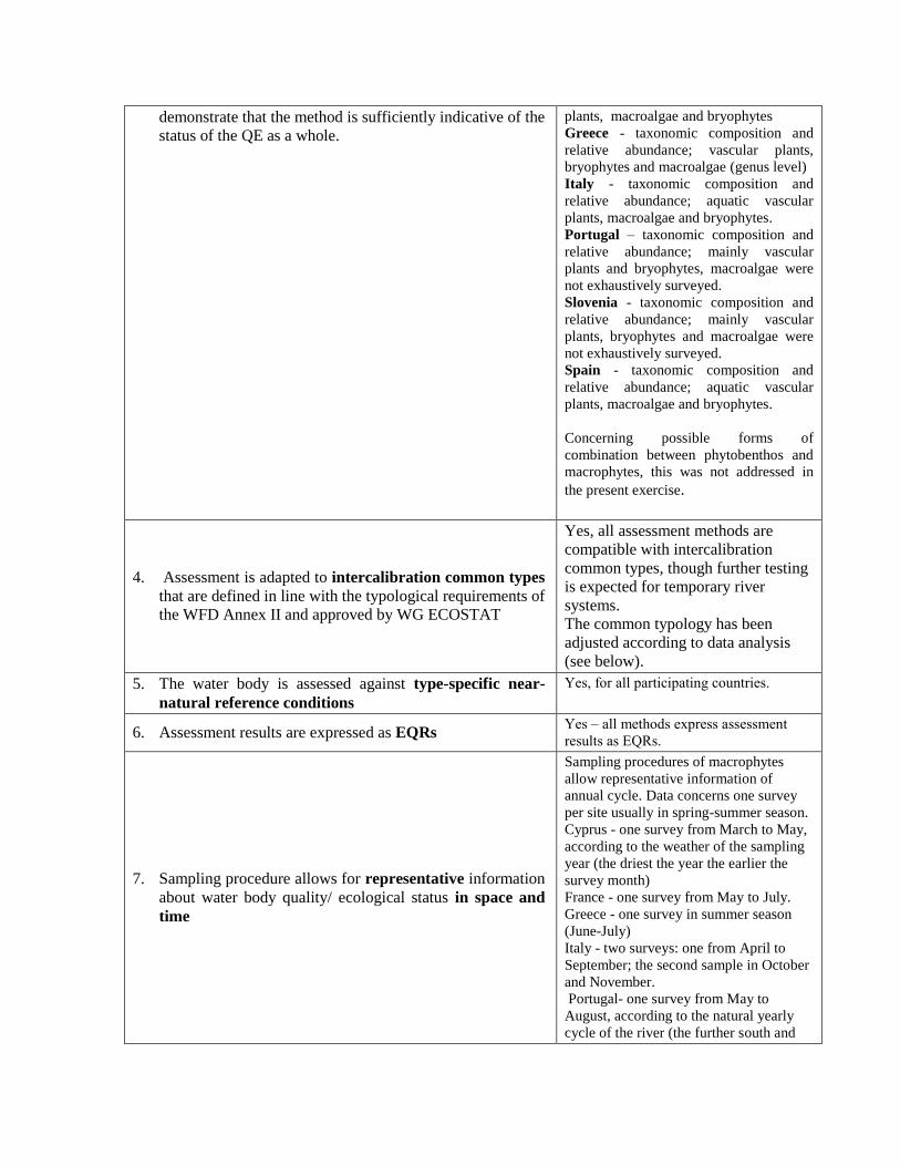
demonstrate that the method is sufficiently indicative of the

status of the QE as a whole.

plants, macroalgae and bryophytes

Greece - taxonomic composition and

relative abundance; vascular plants,

bryophytes and macroalgae (genus level)

Italy - taxonomic composition and


plants, macroalgae and bryophytes.

Portugal – taxonomic composition and

relative abundance; mainly vascular

plants and bryophytes, macroalgae were

not exhaustively surveyed.

Slovenia - taxonomic composition and

relative abundance; mainly vascular

plants, bryophytes and macroalgae were

not exhaustively surveyed.

Spain - taxonomic composition and


plants, macroalgae and bryophytes.

Concerning possible forms of

combination between phytobenthos and

macrophytes, this was not addressed in

the present exercise.

4. Assessment is adapted to intercalibration common types

that are defined in line with the typological requirements of

the WFD Annex II and approved by WG ECOSTAT

Yes, all assessment methods are

compatible with intercalibration

common types, though further testing

is expected for temporary river

systems.

The common typology has been

adjusted according to data analysis

(see below).

5. The water body is assessed against type-specific near-

natural reference conditions

Yes, for all participating countries.

6. Assessment results are expressed as EQRs Yes – all methods express assessment

results as EQRs.

7. Sampling procedure allows for representative information

about water body quality/ ecological status in space and

time

Sampling procedures of macrophytes

allow representative information of

annual cycle. Data concerns one survey

per site usually in spring-summer season.

Cyprus - one survey from March to May,

according to the weather of the sampling

year (the driest the year the earlier the

survey month)

France - one survey from May to July.

Greece - one survey in summer season

(June-July)

Italy - two surveys: one from April to

September; the second sample in October

and November.

Portugal- one survey from May to

August, according to the natural yearly

cycle of the river (the further south and

higher altitude the site, the earlier the

survey).

Spain – one survey from July to

September.

Slovenia - one survey from July to

September

8. All data relevant for assessing the biological parameters

specified in the WFD’s normative definitions are covered

by the sampling procedure

Both relevant parameters of BQE are

covered (i.e. species composition and

abundance). Bryophytes and macroalgae

were only diagnostically assessed in some

cases. Sampling is performed at the peak

growth period thus insuring a good

representative image of the site.

9. Selected taxonomic level achieves adequate confidence

and precision in classification

Species level is required for most of taxa,

which is considered adequate to achieve

confidence and precision in classification.

Genus level is accepted only for

macroalgae due to a limited existence of

taxonomic keys in many cases.

Clarify if there are still gaps in the national method descriptions information.

Summarise the conclusions of the compliance checking:

There is yet some work to be done concerning taxonomy and individual response to

pressures with macroalgae and bryophytes in Mediterranean regions, contrarily to

vascular plants. More basic research has to be conducted in order to have fully

operational methods including macroalgae and also bryophytes. Macroalgae includes

various categories of algae e.g. Charophytes (Chara sp.), red algae (Batrachosperum sp.),

green algae and filamentous algae (e.g. Cladophora sp., Chaetomorpha sp.). Macroalgae

react differently in time and space comparing to angiosperms and some of them are able

to tolerate the drought event. Generally the higher taxonomic plants (angiosperms) react

within years to changes in degradation whereas algae can react within days or even hours.

This characteristic of the green algae can be especially relevant in the evaluation of the

ecological status of temporary Mediterranean rivers (type RM5) where the water course

can partially or totally dry out during the warm period. The presence of vast amounts of

green filamentous algae, occupying the habitats of vascular plants only occur in poor and

bad conditions, therefore can be assumed irrelevant in the present exercise.

There are technical difficulties for determining absolute abundance during sampling, and

relative abundances are generally judged adequate, namely in methods already used for

many years, such as the IBMR method that most countries are using in the present

exercise.

The assessment methods of the MS were considered compliant and ready for

intercalibration.

4. Methods’ intercalibration feasibility check

Do all national methods address the same common type(s) and pressure(s), and follow a similar

assessment concept? (Question 2 in the IC guidance)

4.1. Typology

Describe common intercalibration water body types and list the MS sharing each type

Common IC type Type characteristics MS sharing IC common type

RM1 catchment <100 km2; mixed

geology (except non-

siliceous); highly seasonal

France, Italy, Portugal, Slovenia, Spain

RM2 catchment 100-1000 km2 ;

mixed geology (except non-


France, Greece, Italy, Portugal, Slovenia,

Spain

RM3 catchment 1000-10000 km2 ;

mixed geology (except


Greece, Portugal, Spain

This type cannot be intercalibrated

because present methods do not cover this

type RM4 non-siliceous streams; highly

seasonal

Cyprus, France, Greece, Italy, Spain

RM5 temporary rivers Cyprus, Italy, Portugal, Slovenia, Spain

Note: The borders of the types were redefined for a better adjustment to the ecological reality.

The redefinition was based on ordination data treatment, and presented, discussed and agreed in

the General Mediterranean GIG meetings. The biological analysis of macrophytes revealed a poor

segregation between types RM1, RM2 and RM4, both for the reference sites (Global R of

ANOSIM =0,263; significance level=0,1%) and for the all sites (Global R of ANOSIM =0,218;

significance level=0,1%). Therefore these types were treated together throughout the IC process.

Mediterranean temporary rivers revealed large structural and functional differences [Aguiar FC,

Cambra J, Chauvin C, Ferreira T, Germ M, Kuhar U, Manolaki P, Minciardi MR, Papastergiadou

E. 2010. Floristic and functional gradients of river plant communities: a biogeographycal study

across the Mediterranean Basin. XV Congress of the Iberian Association of Limnology, 5-7 July

2010, Azores: 55], such as richness of hygrophytes, ratio hydrophytes/helophytes and species

diversity and will be subject to a separate data treatment.

What is the outcome of the feasibility evaluation in terms of typology? Are all assessment

methods appropriate for the intercalibration water body types, or subtypes?

Method Appropriate for IC types / subtypes

RMI Appropriate to types RM1, RM2 and RM5

IBMR Appropriate to all types, exceptions: RM3, RM5 of Cyprus.

MMI Appropriate to type RM5

Conclusion Is the Intercalibration feasible in terms of typology?

1 – feasible. Methods can be implemented for all common types, except for RM3.

4.2. Pressures

Describe the pressures addressed by the MS assessment methods. Note: the information for this

Table was provided by each MS, or collected from the WISER report in the cases where the

method was reported.

Method Pressure Remarks

RMI (Slovenia) Catchment land use, Eutrophication

IBMR (Cyprus, Greece,

France, Italy, Portugal,

Spain)

Cyprus –hydrological,

morphological, land-use and

physico-chemical degradation.

Greece - hydrological,

morphological, land use and


France - Eutrophication, General

degradation, Hydromorphological

degradation; Italy –Eutrophication, General

degradation, Pollution by organic

matter;

Portugal – Eutrophication, General

degradation.

Spain - Eutrophication, General

degradation.

MMI (Cyprus) Cyprus – hydrological,

morphological, land use and


Conclusion Is the Intercalibration feasible in terms of pressures addressed by the methods?

IBMR, RMI and MMI address similar types of pressures; however with MedGIG database national

methods have a general low correlation with eutrophic pressures.

The above table refers to the information gathered in WISER report or provided by each MS to

the Mediterranean rivers GIG coordination.

For common data, the Mediterranean GIG database was used to test the response of the each

metric to: individual types of pressures and to a general degradation gradient (obtained from

PCA axes scores). The existence of many gaps in the quantitative data prejudiced the analysis

of relations to pressure, especially concerning physico-chemical variables.

For RM1,2,4 type, the PCA based on pressure data of morphological variables and land-use of

the MedGIG showed that the PCA axis 1 explain 56.4% of the total variation (100% for the

first three axes), and the Pearson correlation coefficient is 0.55 (p<0.000001).

Responses to individual gradients are illustrated bellow:

Fig.1 Response of assessment methods (IC types RM1,2,4) to individual pressures

For RM5, the PCA based on pressure data of morphological variables, hydrological variables

and pH showed that the PCA axis 1 explain 57.7% of the variation, the Pearson correlation

coefficient is 0.58 (p<0.000001). Concerning individual pressures the R (p<0.0001), for

“upstream dams” = -0.63, R “water abstraction” =-0.54; Stream hydrology =0.44, habitat

alteration= -0.38.

4.3. Assessment concept

Do all national methods follow a similar assessment concept?

Examples of assessment concept:

Different community characteristics - structural, functional or physiological - can be

used in assessment methods which can render their comparison problematic. For

example, sensitive taxa proportion indices vs species composition indices.

Assessment systems may focus on different lake zones - profundal, littoral or

sublittoral - and subsequently may not be comparable.

Additional important issues may be the assessed habitat type (soft-bottom sediments

versus rocky sediments for benthic fauna assessment methods) or life forms (emergent

macrophytes versus submersed macrophytes for lake aquatic flora assessment

methods)

1 2 3 4

habitat alteration

0,0

0,4

0,8

1,2

1,6

1 2 3 4

urbanisation

0,0

0,4

0,8

1,2

1,6

1 2 3 4

channelisation

0,0

0,4

0,8

1,2

1,6

assessm

ent m

eth

od

0,0 22,5 45,0 67,5 90,0

extensive agriculture (%)

0,0

0,4

0,8

1,2

1,6

ass

ess

me

nt

me

tho

d

3,5 27,6 51,8 75,9 100,0

semi-natural areas (%)

0,0

0,4

0,8

1,2

1,6

ass

ess

me

nt

meth

od

1 2 3 4

agriculture

0,0

0,4

0,8

1,2

1,6

assessm

ent m

eth

od

Method Assessment concept Remarks

RMI Indicator species based Multihabitat sampling, channel and inner banks

IBMR Indicator species based Multihabitat sampling, channel and inner banks

MMI Based in functional plant

groups

Multihabitat sampling, all channel and inner banks

Conclusion

Is the Intercalibration feasible in terms of assessment concepts?

The intercalibration is feasible in terms of assessment concepts. However, RMI and IBMR has

similar assessment concept concerning the sampling method, though for RMI the indicator species

are mainly spermatophytes and pteridophytes. The indicator value of the species (score) is derived

from presence and abundance of species that showed a correlation with pressure gradient. The MMI

has a different concept (based on functional plant groups), though sampling has the same conceptual

basis, and the index can be applied to other countries.

5. Collection of IC dataset

Describe data collection within the GIG. This description aims to safeguard that compiled data

are generally similar, so that the IC options can reasonably be applied to the data of the Member

States.

Table 5.1 Total number of sites provided by Member States (including RM3):

Member State Biological data Physico- chemical data Other pressure

data

Value of the

assessment

method and

classification

Cyprus 57 57 57 57 France 37 33 37 37

Greece 43 42 43 32

Italy 83 83 83 83

Portugal 120 120 120 90 Slovenia 25 19 25 25

Spain 108 114 114 108

Sum 473 468 479 432

Table 5.2 Total number of national reference sites provided by Member States:

Member State RM1 RM2 RM4 RM5 Total

Cyprus - - 3 8 11

France 10 - 17 - 27

Greece - 13 1 - 14

Italy 5 0 12 0 17

Portugal 10 10 - 9 29

Slovenia 0 0 - 0 0

Spain 10 1 28 0 39

Sum 35 24 61 17 137

Table 5.3 Number of sites provided for each IC common type (Note: some samples collected too

late during growth season were discarded).

IC type Member

State

Biological data

and classification

Physico-

chemical data

Other

pressure data

RM1 France 12 10 12

Italy 25 25 25

Portugal 30 30 30

Slovenia 6 6 6

Spain 10 10 10

Sum 83 81 83

RM2 Greece 31 34 35

Italy 9 9 9

Portugal 30 30 30

Slovenia 15 9 15

Spain 10 11 11

Sum 95 93 100

RM3 Greece 7 7 7

Portugal 30 30 30

Spain 20 20 20

Sum 57 57 57

RM4 Cyprus 14 14 14 France 25 23 25 Greece 1 1 1 Italy 36 36 36 Spain 64 64 64

Sum 140 138 140

RM5 Cyprus 43 43 43 Italy 13 13 13 Portugal 30 30 30 Slovenia 4 4 4 Spain 4 9 9

Sum 94 99 99

List the data acceptance criteria used for the data quality control and describe the data acceptance

checking process and results

Data acceptance criteria Data acceptance checking

Data requirements (obligatory and

optional)

All countries delivered geographical location and river

typology, as well as biological and environmental data, and

also pressure data. The data was organized under the same

agreed frame. Checking included the assessment of the

“mediterranicity” of the sites, that is, the degree of water

availability during summer.

Reference dataset for most of countries is reasonably

complete in pressure and environmental data. There were however gaps in the database, notably in

physico-chemical data. Also for some sites in most

countries, the physico-chemical data is qualitative or if

quantitative, the value is referred just as below or above the

LD; gaps on pressures vary in the type of parameter between

countries and within countries.

The sampling and analytical

methodology

Sampling methods are similar for most countries, however

the inner bank may or may not be included in the surveys;

other differences detected concern the inclusion or not of

bryophytes and macroalgae.

Level of taxonomic precision

required and taxalists with codes

All vascular plants were identified at the species level.

However, the number of species related to water is very

small when compared to helophytes and other waterlogged

species, depending on the country and increasing with

latitude and temporality of the system.

All the biological information and lists of species provided

by the MS had to be compared, harmonized and the final

result agreed by all MS in the GIG meetings.

The procedure was as followed:

All MS delivered taxa lists with similar taxonomic precision

(species level for most of the species), codes and synonymy

were defined at the coordination level. Preparatory included

the harmonization of the database, especially concerning

problems in synonym, and the harmonization of the cover

scale (three different cover scales for the seven countries).

All countries assigned a floristic group for each species

(algae, bryophyte moss, bryophyte hepatic, pteridophyte,

spermatophyte, lichen, heterotrophic organism (fungi &

bacteria) and attributed an “aquaticity” level for all taxa

recorded [C. Chauvin in Birk S., N Willby, C Chauvin, HC

Coops, L. Denis, D. Galoux, A. Kolada, K. Pall, I. Pardo, R. Pot,

D. Stelzer. 2007. Report on the Central Baltic River GIG

Macrophyte Intercalibration Exercise, June 2007].

MedGIG macrophyte coordination harmonized the

classification done by MS for common species. For data

treatment only species with aquaticity level 5 or lower were

accepted, in order to achieve comparable biological

information. From the 736 species gathered in the original

MedGIG, around 40% were eliminated (woody riparian

species, brackish water or salty marsh species, terrestrial

ruderals and grasses). Species codes were attributed using

the CEMAGREF codes in order to be included in the CEN

database. New codes were assigned and suggested; the

information was delivered to CEMAGREF-Bordeaux.

The minimum number of sites /

samples per intercalibration type

Minimum of 15 sites per IC type are available.

Sufficient covering of all relevant All 5 quality classes are represented. However, the database

quality classes per type included few sites classified as poor and bad quality classes,

especially for the RM1,2,4 type.

Fig. 5.1. Distribution of MedGIG macrophyte database samples by

quality class (5 classes) taking into account national EQR values

per type. RM1, RM2, RM4 are shown together.

6. Benchmarking: Reference conditions or alternative benchmarking

In section 2 of the method description of the national methods above, an overview has to be

included on the derivation of reference conditions for the national methods. In section 6 the

checking procedure and derivation of reference conditions or the alternative benchmark at the

scale of the common IC type has to be explained to ensure the comparability within the GIG.

Clarify if you have defined

- common reference conditions (Y)

- or a common alternative benchmark for intercalibration (N)

6.1. Reference conditions

Does the intercalibration dataset contain sites in near-natural conditions in a sufficient number

to make a statistically reliable estimate? (Question 6 in the IC guidance)

- Summarize the common approach for setting reference conditions (true reference sites or

indicative partial reference sites, see Annex III of the IC guidance):

Spatially-based reference sites exist in the common data base for all IC types, except RM3;

the reference sites were those non or minimally disturbed found in the Mediterranean region.

The common reference conditions approach will be used.

- Give a detailed description of reference criteria for screening of sites in near-natural

conditions (abiotic characterisation, pressure indicators):

The Mediterranean GIG has developed common reference conditions. Following data

treatment by Maria João Feio, a proposal for reference conditions thresholds was brought to

the General GIG meetings, and intensively discussed till a final collective decision was made.

All quality values from all countries were then recalculated to comply with these common

thresholds. The same and common thresholds were used for the BQEs macroinvertebrates,

phytobenthos and macrophytes.

For the common approach in the GIG, the selection of IC reference sites was done through a

3 step procedure. Steps 1 and 2, up to the establishment of reference thresholds, were

exclusively performed with the original MS reference sites provided to the MedGIG database.

We used sites supplied to the MedGIG for invertebrates, diatoms and macrophytes databases.

The global database was composed of a total of 919 member states reference samples

distributed through the 4 IC river types (RM1, RM2, RM4, RM5) and 7 MS (Cyprus, France,

Greece, Italy, Portugal, Slovenia, Spain).

Step 1. Reference sites are chosen if all their categorical variables have only class 1, no

impact or minimal impact.

Step 2. Reference thresholds are calculated for numerical pressure variables, based on

reference sites selected in Step 1 and for each IC type. Extreme values for each pressure

variable and IC type were previously excluded after histograms and boxplots inspection.

These observed ranges characterize the pressure levels existent in the minimally disturbed

sites, for each IC type, in the Mediterranean region.

A unique value for each pressure variable (Reference thresholds) was afterwards calculated

for all IC types, corresponding to the maximum pressure acceptable overall Mediterranean

types, in order to reach a common tolerance level. However, for RM5, the temporary rivers,

different ranges for water oxygenation were established for low water periods.

The following table describes the thresholds established and applied:

Table 6.1. Common thresholds established for each pressure variable and used by the

MEDGIG phytobenthos for IC. The values are common to all IC types except for O2, with a

different limit for RM5.

References are accepted if

Pressure variables RM1+RM2+RM4 RM5

General Morphology (Classes 1-3)

General Hydrology (Classes 1-3) ≤ 2

Riparian Vegetation (Classes 1-3)

DO (mg/L) 1 6,39-13,70

O2 (%) 73,72-127,92 60,34-127,92

N-NH4+

(mg/L) ≤0,09

N-NO3- (mg/L) ≤1,15

P-Total (mg/L) ≤0,07

P-PO43-

(mg/L) ≤0,06

% Artificial areas (catchm) ≤1

% Intensive agriculture (catchm) ≤11

% Extensive agriculture (catchm) ≤32

% Semi-natural areas (catchm) ≥68

% Urbanisation (reach) 2

≤1

% Land use (reach) 2 ≤20

% Agriculture (reach) 2 ≤20

1 for macrophytes only, instead of O2 (%)

2 for diatoms only, instead of land use in the catchment

Step 3. Final abiotic screening of reference sites. Potential reference sites, left out in Step I,

are rescreened and those with categorical variables in class 2 (any number) but

simultaneously with numerical variables values within the thresholds defined in Step II are

chosen and added to the reference set of Step 1.

Finally, in order to recover samples for the macrophyte reference database, the entire

database was rescreened for all MS and all types. If samples passed the thresholds for an IC

reference they were also included in the set of benchmarks.

- Identify the reference sites/samples for each Member State in each common IC type.

Table 6.2 Number of IC reference samples selected abiotically using the described procedure, for

intercalibration for macrophytes from entire macrophyte data base and percentage of samples

retained in relation to the total reference samples provided by the MS.

Member

State RM1 RM2 RM4 RM5 Total

Cyprus - - - - 3 100% 5 63% 8 73%

France 6 60% - - 10 59% - - 16 59%

Greece - - 9 69% 1 100% - - 10 71%

Italy 4 80% - - 11 92% - - 15 88%

Portugal 8 80% 5 50% - - 3 33% 16 55%

Slovenia 0 - 0 - - - 0 - - -

Spain 5 50% 0 0% 16 57% 0 0% 21 54%

Sum 23 66% 14 58% 41 67% 8 47% 86 63%

Identify the reference sites for each Member State in each common IC type. Is their number

sufficient to make a statistically reliable estimate?

River types RM1, RM2 and RM4 will be gathered for the intercalibration, and a sufficient

number of reference sites are available to make a statistically reliable estimate. For RM5 the

number of available reference sites can be insufficient (8 sites for the overall database).

- Explain how you have screened the biological data for impacts caused by pressures not

regarded in the reference criteria to make sure that true reference sites are selected:

In order to be sure that the reference sites selected were not influenced by pressures we ran

Spearman rank correlations between pressure variables and EQR values for reference sites,

assuming that these correlations should be low. For RM5 the analyses are not statistically

steadfast for the MedGIG reference dataset; i.e. values of the correlations for pressure

variables for the RM5 reference sites are low both for qualitative and quantitative variables.

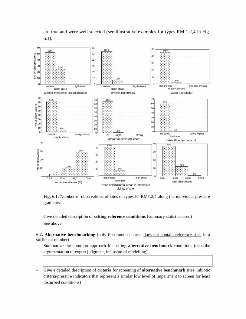
- Further screening data proceed. The high percentage of observations that indicates no

or low alterations in morphological and hydrological pressures, and low values for

eutrophication variables (Spearman rho, p<0.001 <0.18) indicates that reference sites

98%

2%

no dykeslow impact

strong impact

dykes (flood protection)

0

10

20

30

40

50

60

70

No o

f obs

99%

1%

no sligth strong

upstream dams influence

0

10

20

30

40

50

60

70

80

No o

f observ

ations

96%

4%

not affectedsligthly affected

strongly affected

water abstraction

0

10

20

30

40

50

No o

f observ

ations

74%

24%

2%

0,004 0,036 0,068 0,100

total phosphorus

0

10

20

30

40

No o

f observ

ations

are true and were well selected (see illustrative examples for types RM 1,2,4 in Fig.

6.1).

-

-

-

-

-

-

-

-

-

-

-

-

-

-

-

-

-

-

-

Fig. 6.1. Number of observations of sites of types IC RM1,2,4 along the individual pressure

gradients.

Give detailed description of setting reference conditions (summary statistics used)

See above

6.2. Alternative benchmarking (only if common dataset does not contain reference sites in a

sufficient number)

- Summarize the common approach for setting alternative benchmark conditions (describe

argumentation of expert judgment, inclusion of modelling)

- Give a detailed description of criteria for screening of alternative benchmark sites (abiotic

criteria/pressure indicators that represent a similar low level of impairment to screen for least

disturbed conditions)

89%

11%

unalteredslightly altered

highly altered

channel morphology

0

10

20

30

40

50

60

No o

f observ

ations

68%

32%

unalteredsligthtly altered

highly altered

Channel profile/cross section alteration

0

10

20

30

40

50

60

No o

f observ

ations

94%

6%

naturalslightly altered

strongly altered

stream hydrology

0

10

20

30

40

50

60

70

80

No o

f observ

ations

85%

15%

not presentlow effect

high effect

Urban and industrial areas in immediatevicinity of site

0

10

20

30

40

No o

f observ

ations

7%

24%

69%

72,9 82,0 91,0 100,0

semi-natural areas (%)

0

10

20

30

40

No o

f observ

ations

- Identify the alternative benchmark sites for each Member State in each common IC type

- Describe how you validated the selection of the alternative benchmark with biological data

- Give detailed description how you identified the position of the alternative benchmark on the

gradient of impact and how the deviation of the alternative benchmark from reference

conditions has been derived

Describe the biological communities at reference sites or at the alternative benchmark,

considering potential biogeographical differences:

See section 8.2

7. Design and application of the IC procedure

7.1. Please describe the choice of the appropriate intercalibration option.

Which IC option did you use?

For the types RM1, RM2 and RM4 (intercalibrated together):

- IC Option 1 - Same assessment method, same data acquisition, same numerical evaluation

(Y)

- IC Option 2 - Different data acquisition and numerical evaluation (N)

- IC Options 3 - Similar data acquisition, but different numerical evaluation (BQE sampling

and data processing generally similar, so that all national assessment methods can reasonably

be applied to the data of other countries) (Y)

Explanation for the choice of the IC option:

We performed the IC Option 1 for six countries of the Mediterranean rivers GIG macrophytes

(Cyprus, France, Greece, Italy, Portugal, Spain) that use the same assessment method (IBMR,

Biological Macrophyte Index for Rivers), same data acquisition and same numerical evaluation.

Then the IC Options 3 - Similar data acquisition, but different numerical evaluation (BQE

sampling and data processing generally similar, so that all national assessment methods can

reasonably be applied to the data of other countries) was performed for the national method of

Slovenia (River Macrophyte Index), using the fixed Median value of the H/G boundary of the

countries intercalibrated previously. This alternative was followed since the RMI cannot be

computed to all sites of the database due to low number of indicator taxa, which specially

occurred for the database of France, Cyprus and Spain. The regression of RMI and the IBMR was

made using sites from Greece, Portugal and Italy (n=103).

The correlation coefficient of the RMI and the IBMR was r=0,6770; p=0.000001.

In case of IC Option 2, please explain the differences in data acquisition

Not applicable

For the type RM5:

Italy, Cyprus, Spain, Slovenia, and Portugal share this intercalibration type. We considered that

only Portugal, Cyprus and Italy had a representative number of sites to intercalibrate (Spain and

Slovenia have only 4 sites). The r value of MMI (Cyprus national method) with the other national

methods (IBMR) was very low (see table below) and did not allow the direct comparison. The

bad correlation between MMI and IBMR was to be expected at least in the Cyprus case, as the

IBMR had been shown not applicable to Cyprus R-M5 using CY data.

Member State/Method r p

Cyprus/ MMI vs. IBMR (IT, CY, PT) 0.045 0.6824

Cyprus/ MMI vs. IBMR (CY, PT) 0.001 0.9376

Cyprus/ MMI vs. IBMR (IT, CY) 0.071 0.6008

The intercalibration procedures described for Option 1 of RM1,2,4 were applied for Italy and

Portugal, and results are presented in Anex 1, however it was agreed that the results are not

reliable, since the database has a small number of sites (30 for Portugal and 13 for Italy) and the

number of reference sites is also low (3 reference sites, all from Portugal). It was concluded that

the intercalibraton was considered not feasible, during the 7th Mediterranean meeting (Madrid,

10-11 October).

7.2. IC common metrics (When IC Options 2 or 3 are used)

Describe the IC Common metric:

Not applicable

Are all methods reasonably related to the common metric(s)? (Question 5 in the IC guidance)

Please provide the correlation coefficient (r) and the probability (p) for the correlation of each

method with the common metric (see Annex V of IC guidance).

Member State/Method r p

Explain if any method had to be excluded due to its low correlation with the common metric:

Not applicable

8. Boundary setting / comparison and harmonization in common IC type

Clarify if

- boundaries were set only at national level (Y)

- or if a common boundary setting procedure was worked out at the scale of the common IC

type (N)

In section 2 of the method description of the national methods above, an overview has to be

included on the boundary setting procedure for the national methods to check compliance with

the WFD. In section 8.1 the results of a common boundary setting procedure at the scale of the

common IC type should be explained where applicable.

8.1. Description of boundary setting procedure set for the common IC type

Summarize how boundaries were set following the framework of the BSP:

Provide a description how you applied the full procedure (use of discontinuities, paired

metrics, equidistant division of continuum)

Not applicable

Provide pressure-response relationships (describe how the biological quality element

changes as the impact of the pressure or pressures on supporting elements increases)

Not applicable

Provide a comparison with WFD Annex V, normative definitions for each QE/ metrics

and type

Not applicable

8.2. Description of IC type-specific biological communities representing the “borderline”

conditions between good and moderate ecological status, considering possible biogeographical

differences (as much as possible based on the common dataset and common metrics).

RM1, RM2 & RM4

In these rivers types, the major changes in the floristic communities between the good and the

moderate ecological status are associated with the decrease of species richness (median in G sites

=12; M sites=7), and an increase in cover and frequency of pondweed taxa, such as Potamogeton

pectinatus and P. nodosus, macroalgae (e.g. Enteromorpha sp., Cladophora sp.), and other

hydrophyes (for instance Lemna gibba), and of some emergent species, such as Schoenoplectus

lacustris. In opposition, there is a loss and/or decrease in cover of bryophytes (both mosses and

liverworts), mainly Rhynchostegium riparioides, Fontinalis antipyretica, Fissidens crassipes,

Eurhynchium praelongum, Lunularia cruciata and Amblistegium riparium, and of some

amphibious and hygrophyte species (Lotus pedunculatus, Carex elata, Carex pendula).

Some infrequent species in the data base, bryophytes (Bryum sp.) , isoetids, Juncus sp., Myosotis

sp. were only observed in sites classified in Good ecological status. Some alien invasive species

also raise their abundance due the raise of pressures, this is the case of Azolla sp.

8.3. Boundary comparison and harmonisation

Describe comparison of national boundaries, using comparability criteria (see Annex V of IC

guidance).

8.3.1 Procedures for the IC of types RM1,2,4

We performed the following steps for translating the national boundaries, define a harmonisation

guideline, evaluation the level of boundary bias, harmonising class boundaries and analyse the

class agreement.

1. Calculate the EQR site values for Mediterranean GIG (MedGIG EQR), using the IBMR

absolute values divided by the median of the IBMR values of MedGIG reference sites

(previously screened with MedGIG criteria; section 6.1).

2. Convert boundaries to IC EQR using regression analyses per MS: MedGIG EQR vs.

National EQR IBMR reference sites.

3. Boundary harmonization using option 1: all countries except SI, IC types RM1, 2, 4. The

boundary bias criterion was used: boundary bias should be less than a quarter of the

width of a class. We used the median of the boundaries to compute the boundary bias.

We changed iteratively the values of the boundaries that did not meet the criteria until the

median of the boundaries was included within the quarter of the class (High or Good).

Convert all harmonized boundaries at the scale of IC EQR IBMR into the absolute IBMR

values (product between IC EQR and the median value of IBMR at MedGIG reference

sites).

4. Boundary harmonization using option 3

4.1 Whenever possible, RMI (Slovenia National Method) was computed for the entire

database. The IBMR was also computed for the Slovenian sites.

4.2 The IBMR was regressed against RMI in order to check the relatedness of indices

and to convert RMI boundaries into the IBMR scale. Only sites from Greece, Italy,

Portugal and Slovenia were used in the regression (Spain, Cyprus and France were

not considered because the RMI was computed for a very small number of sites).

4.3 The boundary bias of RMI (after conversion to the IC EQR IBMR scale using the

regression equation) was computed using the median values after option 1 boundary

harmonization. In case the RMI boundaries did not meet the criteria (boundary bias

lower than a quarter of a class), these were moved until the median of the boundaries

(computed in step 3) was included within a quarter of a class.

4.4 Convert the harmonized boundaries at the IC EQR IBMR scale into RMI values

using the inverse function of the regression equation.

5. Class agreement was computed for all pair combination of National method. Only sites

that were classified as H, G or M according to both National Methods were used to

compute class agreement. First, a piecewise transformation of the IC EQR IBMR values

was performed using the formula:

MinT – ((X – Min)*0.2) / (Max – Min)

, where MinT – Minimum of the new transformed class (0.6 for G and 0.8 for H), X –

index value, Min –theoretical index minimum, Max – theoretical index maximum.

Class agreement was computed as the mean absolute difference between the index values

after piecewise transformation divided by 0.2 (the width of each class after piecewise

transformation). Class agreement should be less than 1 (meaning that the mean

differences should be less than the width of 1 class).

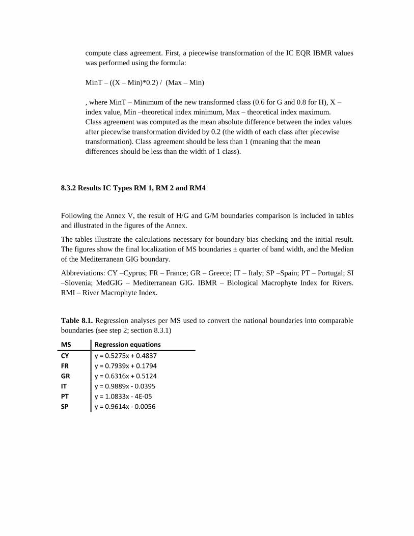
8.3.2 Results IC Types RM 1, RM 2 and RM4

Following the Annex V, the result of H/G and G/M boundaries comparison is included in tables

and illustrated in the figures of the Annex.

The tables illustrate the calculations necessary for boundary bias checking and the initial result.

The figures show the final localization of MS boundaries ± quarter of band width, and the Median

of the Mediterranean GIG boundary.

Abbreviations: CY –Cyprus; FR – France; GR – Greece; IT – Italy; SP –Spain; PT – Portugal; SI

–Slovenia; MedGIG – Mediterranean GIG. IBMR – Biological Macrophyte Index for Rivers.

RMI – River Macrophyte Index.

Table 8.1. Regression analyses per MS used to convert the national boundaries into comparable

boundaries (see step 2; section 8.3.1)

MS Regression equations

CY y = 0.5275x + 0.4837

FR y = 0.7939x + 0.1794

GR y = 0.6316x + 0.5124

IT y = 0.9889x - 0.0395

PT y = 1.0833x - 4E-05

SP y = 0.9614x - 0.0056

Table 8.2. Boundary values used for boundary harmonization; original national boundary values

are in Anex 1.

CY FR GR IT PT SP

Max 1.0112 1.3935 1.1440 1.2263 1.4435 1.3859 H/G 0.9031 0.9177 0.9861 0.8505 0.9966 0.9077 G/M 0.7981 0.8066 0.8661 0.7516 0.7474 0.6770 M/P 0.6931 0.7034 0.7461 0.6033 0.4983 0.4463 P/B 0.5881 0.5922 0.6324 0.4550 0.2491 0.2251

Table 8.3. IC results Option 1 with original boundaries for H/G and G/M boundary (values of

original boundaries were regressed using MedGIG reference data values for each MS). High Max

- maximum of national EQR.

CY FR GR IT PT SP

Max 1.011 1.393 1.144 1.226 1.443 1.386

MedGIG_H/G 0.903 0.918 0.986 0.851 0.997 0.908

MedGIG_G/M 0.798 0.807 0.866 0.752 0.747 0.677

MedGIG_M/P 0.693 0.703 0.746 0.603 0.498 0.446

MedGIG_P/B 0.588 0.592 0.632 0.455 0.249 0.225

H width to Max 0.11 0.48 0.16 0.38 0.45 0.48

G width 0.10 0.11 0.12 0.10 0.25 0.23

M width 0.10 0.10 0.12 0.15 0.25 0.23

H/G bias -0.01 0.00 0.07 -0.06 0.08 0.00

G/M bias 0.02 0.03 0.09 -0.02 -0.03 -0.10

H/G bias_CW -0.09 0.04 0.61 -0.17 0.34 -0.01

G/M bias_CW 0.22 0.31 0.76 -0.23 -0.11 -0.42

Table 8.4 Median value of the MedGIG MS using IBMR as national method for H/G and G/M

boundaries

Median MedGIG

H/G 0.9127

G/M 0.7749

Fig. 8.1 Illustrative results of boundary comparison 8.1a) H/G original Boundaries; 8.1b) G/M

original Boundaries (converted using MedGIG reference data)

Table 8.5. IC results Option 1 with harmonized boundaries for H/G and G/M boundary (values of


- maximum of national EQR.

CY FR GR IT PT SP

Max 1.011 1.393 1.144 1.226 1.443 1.386

MedGIG_H/G 0.903 0.918 0.928 0.851 0.967 0.908

MedGIG_G/M 0.774 0.771 0.757 0.752 0.747 0.709

MedGIG_M/P 0.693 0.703 0.746 0.603 0.498 0.446

MedGIG_P/B 0.588 0.592 0.632 0.455 0.249 0.225

H width to Max 0.108 0.476 0.216 0.376 0.476 0.478

G width 0.129 0.147 0.171 0.099 0.220 0.199

M width 0.081 0.068 0.011 0.148 0.249 0.263

H/G bias -0.010 0.005 0.015 -0.062 0.054 -0.005

G/M bias 0.020 0.017 0.003 -0.003 -0.007 -0.045

H/G bias_CW -0.09 0.03 0.09 -0.17 0.25 -0.01

G/M bias_CW 0.24 0.25 0.25 -0.03 -0.03 -0.23

Table 8.6. Median value of the MedGIG MS using IBMR as national method for H/G and G/M

boundaries

Median MedGIG

H/G 0.9127

G/M 0.7543

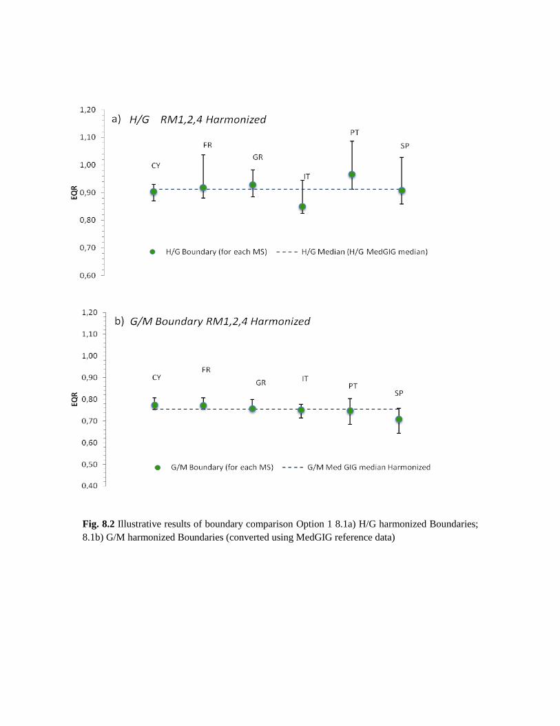
Fig. 8.2 Illustrative results of boundary comparison Option 1 8.1a) H/G harmonized Boundaries;

8.1b) G/M harmonized Boundaries (converted using MedGIG reference data)

Table 8.7 Conversion to the national boundary values (using the regression equations).

CY: x=( - 0.4837)/0.5275); FR: x = (y- 0.1794)/0.7939; GR: x = (y - 0.5124)/0.6316; PT: x= (y +

4E-05)/1.0833; SP: x=(y+0.0056)/0.9614.

CY FR GR IT PT SP

Harmonized boundaries (MedGIG scale)

H/G 0.9031 0.9177 0.9861 0.8505 0.9966 0.9077 G/M 0.7981 0.8066 0.8661 0.7516 0.7474 0.6770

Harmonized boundaries (national scale)

H/G 0.795 0.93 066 0.90 0.89 0.95 G/M 0.550 0.75 0.39 0.80 0.69 0.74

Boundary comparison and harmonization is summarized in Table 9.1, as well as a summary of

results.

For the intercalibration of national method of Slovenia for the BQE macrophytes (River

Macrophyte Index, RMI), Option 3 was used. Figure 8.3 shows the regression of EQR values of

IBMR calculated with MedGIG reference data (EQR_IBMR_MedGIG) and EQR values of RMI

calculated with MedGIG reference data (EQR_RMI_MedGIG). Sites values used are from

Greece, Italy, Portugal and Slovenia; n=103.

Fig. 8.3 Scatterplot showing the regression of EQR values of IBMR calculated with MedGIG

reference data (EQR_IBMR_MedGIG) and EQR values of RMI calculated with MedGIG

reference data (EQR_RMI_MedGIG).

Table 8.8 Boundary values used for boundary harmonization; original national boundary values

are in Anex 1. RMI_BS (benchmark standardized - RMI boundary values calculated with the

median values of the MedGIG reference data. RMI_reg IBMR

RMI RMI_BS RMI_reg IBMR

Max 1.1925 H/G 1.4454 0.8814 G/M 0.9412 0.7363 M/P 0.7059 0.5910 P/B 0.4706 0.4459 Min 0.2353 0.3007

Table 8.9 IC results Option 1 with harmonized boundaries for H/G and G/M boundary (values of


- maximum of national EQR. The harmonized Median value H/G and G/M (see table 8.6) was

fixed to intercalibrate RMI.

SI

Max 1.1925 MedGIG_H/G 0.8814 MedGIG_G/M 0.7363 MedGIG_M/P 0.5910 MedGIG_P/B 0.4459

H width to Max 0.311

G width 0.145

M width 0.145

H/G bias -0.031

G/M bias -0.018

H/G bias_CW -0.101

G/M bias_CW -0.125

Fig. 8.4 Illustrative results of boundary comparison Option 1 8.1a) H/G harmonized Boundaries;

8.1b) G/M harmonized Boundaries (converted using MedGIG reference data)

Do all national methods comply with these criteria ? (N)

If not, describe the adjustment process:

Some national methods did not comply with the comparability criteria. Boundary bias is exceeded

by the methods of:

Greece: H/G boundary (too stringent)

Portugal: H/G boundary (too stringent)

Cyprus: G/M boundary (too stringent)

Greece: G/M boundary (too stringent)

France: G/M boundary (too stringent)

Spain: G/M boundary (too relaxed)

The boundary bias criterion was used: boundary bias should be less than a quarter of the width of

a class. We used the median of the boundaries to compute the boundary bias. We changed

iteratively the values of the boundaries that did not meet the criteria until the median of the

boundaries was included within the quarter of the class (High or Good).

The required boundary adjustments are specified in the table below. Spain agreed to raise the H/G

boundary to comply with the comparability criteria. The countries (Cyprus, Greece, Portugal and

France) can lower the national boundaries, but preferred to maintain the original national values

before the harmonization. The average absolute class difference after boundary adjustment meets

the comparability criteria for all national methods.

9. IC results

Provide H/G and G/M boundary EQR values for the national methods for each type in a table

Table 9.1 National class boundaries and boundaries bias adjustment (adjusted boundaries if bias

>|0.25|). Proposed adjustments: ↑ boundary to be raised, ↓ boundary can be lowered. Final

accepted boundaries for MS.

RM1,2,4

Original

Adjusted Final agreed national boundaries

H/G G/M H/G

G/M

H/G G/M

Cyprus Boundary 0.795 0.596

0.550 ↓ 0.795 0.596

Bias CW -0.09 0.22

0.24

France Boundary 0.93 0.79

0.745 ↓ 0.93 0.79

Bias CW 0.04 0.31

0.25

Greece Boundary 0.75 0.56 0.66 ↓ 0.39 ↓ 0.75 0.56

Bias CW 0.61 0.76 0.09

0.25

Italy Boundary 0.90 0.80

0.90 0.80

Bias CW -0.17 -0.23

Portugal Boundary 0.92 0.69 0.89 ↓

0.92 0.69

Bias CW 0.34 -0.11 0.25

Spain Boundary 0.95 0.71

0.74 ↑ 0.95 0.71*

Bias CW -0.01 -0.42

-0.23

Slovenia Boundary 0.80 0.60

0.80 0.60

Bias CW -0.101 -0.125

*waiting for final official agreement; agreement of macrophyte experts and national

representatives

Present how common intercalibration types and common boundaries will be

transformed into the national typologies/assessment systems (if applicable)

We converted the harmonized boundaries at the IC EQR IBMR original boundaries using the

regression equation obtained. Final boundaries were computed for the MS that have boundary

adjustments to comply with the harmonization criteria.

At the MS level, the harmonized values will be adapted to the original national assessment

methods.

Indicate gaps of the current intercalibration. Is there something still to be done?

All goals for intercalibration work programme 2008-2011 dated from 24th September 2008,

were achieved, namely translation of IC results into national systems, refinement of criteria

for setting reference conditions between MS, intercalibration of national methods,

intercalibration of most pressures, the differences of macrophyte communities and its

importance in temporary rivers.

However, large rivers (RM3) and temporary rivers (RM5) were not intercalibrated. See

sections 4.1 and 7.1, respectively.

Annex 1. Original national boundaries of MS. IBMRBiological Macrophytes Index for

Rivers; RMI – River Macrophyte Index

Method IBMR RMI

MS CY FR GR IT PT SP SI

Max 1 1.5292 1 1.2800 1.3325 1.4474 1

H/G 0.795 0.93 0.75 0.90 0.92 0.95 0.80

G/M 0.596 0.79 0.56 0.80 0.69 0.71 0.60

M/P 0.397 0.66 0.37 0.65 0.46 0.47 0.40

P/B 0.198 0.52 0.19 0.50 0.23 0.24 0.20

Anex 2. Results IC Option 1 RM5

Anex 2.1 Boundaries for countries that share RM5 IC type.

Method MMI IBMR RMI

MS CY IT PT SI

H/G 0.880 0.90 0.93 0.80

G/M 0.660 0.80 0.70 0.60

M/P 0.440 0.65 0.46 0.40

P/B 0.220 0.50 0.23 0.20

Anex 2.2

Original boundaries (national scale and regressed).Regression analyses per MS used to convert

the national boundaries into comparable boundaries.´- IT: Y=0.8674x+0.1655; PT:

0.9999+0.0002

Boundaries Original Original MedGIG

IT PT IT PT

Max 1.1240 1.1538 1.1405 1.1535

H/G 0.90 0.93 0.946 0.930

G/M 0.80 0.70 0.859 0.700

M/P 0.65 0.46 0.729 0.460

P/B 0.50 0.23 0.599 0.230

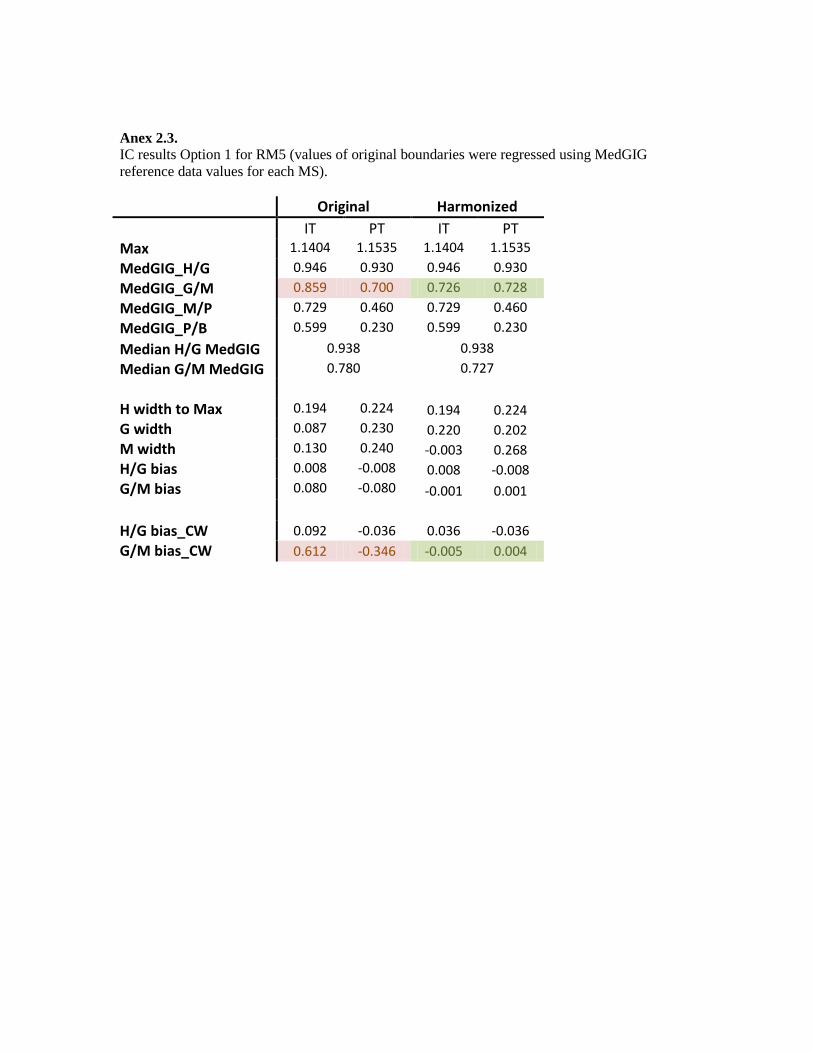
Anex 2.3.

IC results Option 1 for RM5 (values of original boundaries were regressed using MedGIG

reference data values for each MS).

Original Harmonized

IT PT IT PT Max 1.1404 1.1535 1.1404 1.1535

MedGIG_H/G 0.946 0.930 0.946 0.930

MedGIG_G/M 0.859 0.700 0.726 0.728

MedGIG_M/P 0.729 0.460 0.729 0.460

MedGIG_P/B 0.599 0.230 0.599 0.230

Median H/G MedGIG 0.938 0.938

Median G/M MedGIG 0.780 0.727

H width to Max 0.194 0.224 0.194 0.224

G width 0.087 0.230 0.220 0.202

M width 0.130 0.240 -0.003 0.268

H/G bias 0.008 -0.008 0.008 -0.008

G/M bias 0.080 -0.080 -0.001 0.001

H/G bias_CW 0.092 -0.036 0.036 -0.036

G/M bias_CW 0.612 -0.346 -0.005 0.004

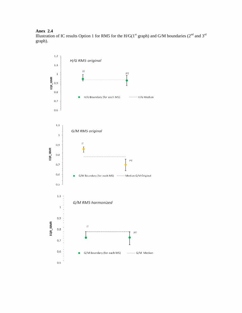
Anex 2.4

Illustration of IC results Option 1 for RM5 for the H/G(1st graph) and G/M boundaries (2

nd and 3

rd

graph).

Anex 2.4. National class boundaries and boundaries bias adjustment for RM5 IC type (adjusted

boundaries if bias >|0.25|). Proposed adjustments: ↑ boundary to be raised, ↓ boundary can be

lowered.

RM5

Original Adjusted

Final agreed national boundaries

H/G G/M H/G

G/M

H/G G/M

Italy Boundary 0,946 0,859

0.726 ↓ Not accepted due to the

small database Bias CW 0.092 0.612

-0.005

Portugal Boundary 0,930 0,700

0.728 ↑ Not accepted due to the

small database Bias CW -0.036 -0.346

0.004

Anex 2.5. Conversion to the national boundary values (using the regression equations).

IT PT

Harmonized boundaries (MedGIG scale)

H/G 0.946 0.929 G/M 0.726 0.728

Harmonized boundaries (national scale)

H/G 0.90 0.93 G/M 0.65 0.73

EUROPEAN COMMISSION DIRECTORATE … Research Centre/jrc...List of national elements attending the...

Documents

Transcript of EUROPEAN COMMISSION DIRECTORATE … Research Centre/jrc...List of national elements attending the...