EULER INTEGRATION OF GAUSSIAN RANDOM FIELDSAND PERSISTENT HOMOLOGYOMER BOBROWSKI & MATTHEW STROM BORMAN

Presented by Roei Zohar

THE EULER INTEGRAL- REASONING

As we know, the Euler characteristic is an additive operator oncompact sets:

which reminds us of a measure

That is why it seems reasonable to define an integral with respect to this “measure”.

BABABA

THE EULER INTEGRAL- DRAWBACK

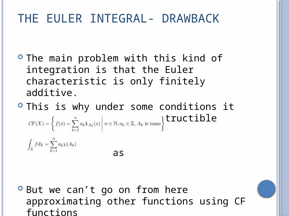
The main problem with this kind of integration is that the Euler characteristic is only finitely additive.

This is why under some conditions it can be defined for “constructible functions”

as

But we can’t go on from here approximating other functions using CF functions

EULER INTEGRAL - EXTENSIONS

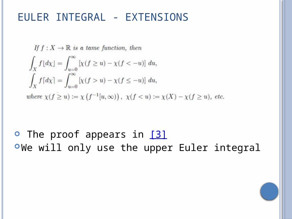
We shall define another form of integration that will be more useful for calculations:

For a tame function the limits are well defined, but generally not equal.

This definition enable us to use the following useful proposition

EULER INTEGRAL - EXTENSIONS

The proof appears in [3]We will only use the upper Euler integral

EULER INTEGRAL - EXTENSIONS

We continue to derive the following Morse like expression for the integral:

FURTHER HELPFUL DEVELOPMENT

GAUSSIAN RANDOM FIELDS AND THE GAUSSIAN KINEMATIC FORMULA

Now we turn to show the GK formula which is

an explicit expression for the mean value of

all Lipschitz-Killing curvatures of excursion

sets for zero mean, constant value variance,

c², Gaussian random fields. We shall not go

into details, you can take a look in [2].

The metric here, under certain conditions is

Under this metric the L-K curvatures are computed in the GKF, and in it the manifold M is bounded

0 Where

,

xfExm

tfsfEtmtfsmsfEtsC TT

When taking we receive and:

Now we are interested in computing the Euler integral of a Gaussian random field:

Let M be a stratified space and let be a Gaussian or Gaussian related random field.We are interested in computing the expected value of the Euler integral of the field g over M.

0i **0

DmMDfE jj

M

j

j

2 dim

12

1

Mg :

Theorem: Let M be a compact d-dimensional stratified space, and let be a k-dimensional Gaussian random field satisfying the GKF conditions. For piecewise c² functionlet setting , we have

kMf :

kG :.fGg

uGDu ,1

mean.constant a has Where

2 1

2

g(t)g

duDmMgEMdgE ujj

d

j

j

M

The proof:

The difficulty in evaluating the expression above lies in computing the Minkowski functionals

In the article few cases where they have been computed are presented, which allows us to simplify , I will mention one of them

Real Valued Fields:

dxxxgxfgf

ex

xdx

dxxH

GGsignHMgEMdgE

x

n

nn

n

j

jj

j

d

j

j

M

,

2

1

2

)(,1

22/1

1

2

1

1

2

And if G is strictly monotone:

d

j j

j

j

M

j

j

j

d

j

j

M

GHMdgE

GHMdgE

02

20

2

, :Decreasing

2

,1 :Increasing

WEIGHTED SUM OF CRITICAL VALUES

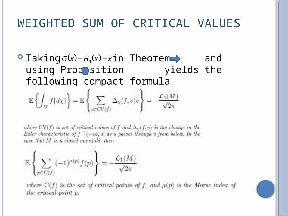
Taking in Theorem and using Proposition yields the following compact formula

xxHxG 1

WEIGHTED SUM OF CRITICAL VALUES

The thing to note about the last result, is that

the expected value of a weighted sum of the

critical values scales like , a 1-

dimensional measure of M and not the

volume , as one might have expected. Remark: if we scale the metric by , then

scales by

M1

Md

Md

k

WE’LL NEED THIS ONE UP AHEAD

The proof relies on

INTRODUCTION : PERSISTENT HOMOLOGY

Have a single topological space, X

Get a chain complex

For k=0, 1, 2, …

compute Hk(X)Hk=Zk/Bk

Ck(X) C1(X) C0(X)Ck-1(X) 0∂ ∂∂ ∂ ∂ ∂

The Usual Homology

INTRODUCTION : PERSISTENT HOMOLOGY

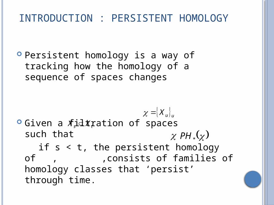
Persistent homology is a way of tracking how the homology of a sequence of spaces changes

Given a filtration of spaces such that

if s < t, the persistent homology of , ,consists of families of homology classes that ‘persist’ through time.

uuXts XX

*PH

INTRODUCTION : PERSISTENT HOMOLOGY

o Explicitly an element of is a family of homology classesfor

o The map induced by the inclusion , maps

kPH t tkt XHbat where,],[

tksk XHXH ts XX

. to ts

Given a tame function

.in elements of sdeath time andbirth tocorespond will valuescritical

hen thefunction t Morse a is iffor theory,Morse oftion generaliza a

asseen becan :function tamea ofhomology persistent The

.,

., spaces of filtration associatedan is there,:

*

1**

1

fPH

f

Xf

ufPHfPH

ufXf

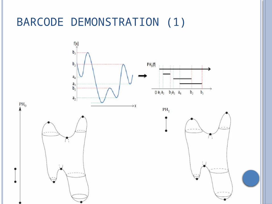
BARCODE DEMONSTRATION (1)

BARCODE DEMONSTRATION (2)

INTRODUCTION : PERSISTENT HOMOLOGY

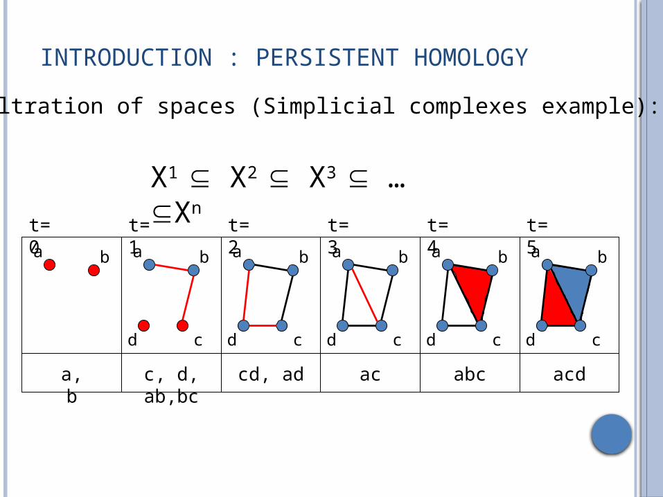
X1 X2 X3 …Xn

a b a b

cd

a b

cd

a b

cd

a b

cd

a b

cd

a, b c, d, ab,bc cd, ad ac abc acd

t=0 t=1 t=2 t=3 t=4 t=5

A filtration of spaces (Simplicial complexes example):

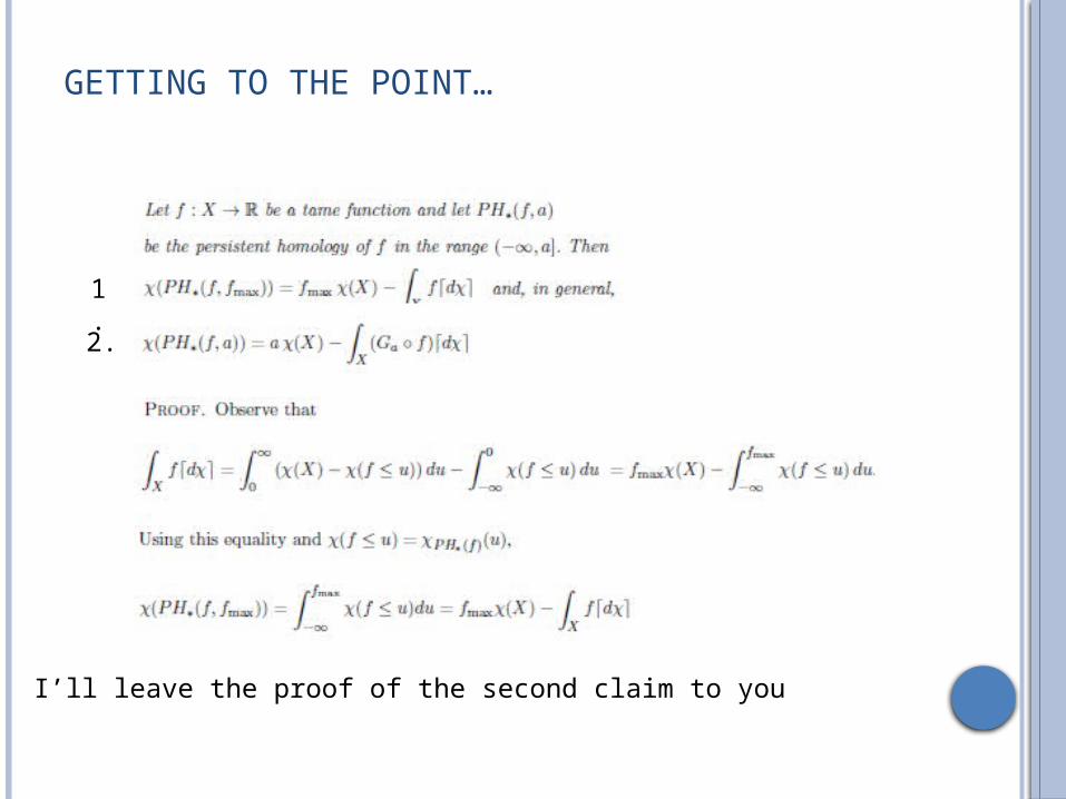
GETTING TO THE POINT…

I’ll leave the proof of the second claim to you

1.

2.

THE EXPECTED EULER CHARACTERISTIC OF THE PERSISTENT HOMOLOGY OF AGAUSSIAN RANDOM FIELD

In light of the connection between the

Euler

integral of a function and the Euler

characteristic of the function’s persistent

homology in place, we will now reinterpret

our computations about the expected Euler

integral of a Gaussian random field

1.

2.

The proof makes use of the following two expressions we saw before:

Computing is not usually possible, but in the case of a real random Gaussian field we can get around it and it comes out that:

max gE

AN APPLICATION – TARGET ENUMERATION

THE END

DEFINITIONS

A “tame” function :

finite. always is ,f of ypehomotopy t theif is

sticcharacteriEuler finite a with X space ltopologica

compact aon X : ffunction continuousA

1- u

tame

REFERENCES

1. Paper presented here, by Omer Bobrowski & Matthew Strom Borman

2. R.J. Adler and J.E. Taylor. Random Fields and Geometry. Springer, 2007.

3. Y . Baryshikov and R. Ghrist. Euler integration over definable functions. In print, 2009.