CHAPTER 1

EUCLIDEAN SPACETIME AND NEWTONIAN PHYSICS

Absolute, true, and mathematicaltime, of itself, and from its ownnature, flows equably withoutrelation to anything external . . .

Isaac NewtonScholium of the Principia

The purpose of this chapter is to remind you the basic features of the Galilean spacetime and itssymmetries, which are closely related to the form taken by Newton’s laws as seen by inertial observers.Although ideas presented in this chapter will be all familiar to you, the way of looking at them willbe probably new. We will introduce some tensorial notation that will be useful in the future. Indeed,local differential geometry can be understood as a refinement of the tensorial methods presented here.

1.1 Galilean Relativity

Newtonian mechanics is based in two basic axioms:

1. Principle of Relativity : The laws of physics are the same in all the inertial frames: No experimentcan measure the absolute velocity of an observer; the results of any experiment do not dependon the speed of the observer relative to other observers not involved in the experiment.

2. There exists an absolute time, which is the same for any observer.

1.2 Euclidean spacetime: old wine in a new bottle

When formulating mechanics in an axiomatic form, Newton, based on everyday experience1, assumedthe spacetime to be Euclidean E1 × E3, i.e. an intrinsically flat and orientable metric space withtrivial topology and well-defined distances and angles. A physical process in this spacetime (suchas the collision of two particles) is called an event and it is independent of the particular choice of

1This is, at velocities much smaller than the velocity of light.

1.2 Euclidean spacetime: old wine in a new bottle 3

t

e 1

e 2

Futu

re

Past

Worl

dline

Past

Future

Worl

dline

Inert

ial obse

rver

Figure 1.1: Galilean spacetime.

coordinates used for its description. The spatial location of the event can be specified in Cartesiancoordinates (x, y, z), in spherical coordinates (r, θ, φ), or making use of any 3 independent numbersobtained by a well-defined coordinate transformation. However, among all the coordinates systemsthat can be used in Newtonian physics, the inertial coordinate systems are privileged (and least forNewton and Galileo). An inertial frame is a frame moving freely in spacetime, free of any force, whichcarries ideal clocks and measuring rods forming an orthonormal Cartesian coordinate system. In sucha frame, a particular event P is characterized by 4 coordinates: its position2

{xi} = {x, y, z} = {x1, x2, x3} , (1.1)

and the time t at which it happens.

Time

Physical time is absolute (up to affine changes, see below) and it is used to characterize particletrajectories xi(t). The temporal separation dt between two events is well-defined, independently oftheir spatial separation (see below). Simultaneous events are characterized by equal time surfacesseparating the future and the past of the events. Any event may cause any simultaneous or laterevent.

Space

For each spatial coordinate we define a set of orthonormal basis vectors along the xi coordinatedirection

ei = {ex, ey, ez} = {e1, e2, e3} , ei · ej = δij , (1.2)

with δij the 3 dimensional Kronecker delta

δij =

1 0 00 1 00 0 1

= diag(1, 1, 1) . (1.3)

2We emphasize here that we do not consider {xi} to be a vector since the homogeneity of space makes the choice ofan origin completely arbitrary. The distance between points is the only significant quantity. On top of that, coordinateswill no longer behave as a vector in the presence of gravity.

1.2 Euclidean spacetime: old wine in a new bottle 4

The infinitesimal displacement vector dX between two points (as any other vector in E3) can beexpanded in terms of the basis vectors ei as

dX =

3∑i=1

dxi ei = dx1 e1 + dx2 e2 + dx3 e3 , (1.4)

with dxi the so-called contravariant components of the vector in that orthonormal basis.

Einstein summation conventionNote the way in which we have located the indices in the previous equation. From now on, anindex appearing twice in a product (in a superscript-subscript combination) will be understoodto be automatically summed on or contracted. A quantity with no free tensor indices is saidto be fully contracted The name of the pair of contracted indices (latin indices (i, j, k, . . .) forthe spatial coordinates or greek ones (µ, ν, ρ, . . .) in 3+1 spacetime dimensions) is completelyarbitrary and can be changed at will. For this reason, these indices are called dummy indices.Expressions with more than two repeated indices should never occur, being necessary in somecases to relabel them in order to avoid ambiguities. Non repeated indices are called free indicesand must appear at the same level at both sides of the equations, for each independent term.As you will see, these rules are very useful, since they will allow us to reconstruct equationswithout any memorization, just by properly setting the indices up or down in the equation. Ontop of that, we will save a lot of time when writing expressions in General Relativity, whichtypically contain lots of indices. Using this convention, Eqs. (1.4) can be written as

dX =

3∑i=1

dxi ei → dX = dxi ei . (1.5)

ExerciseWhich of the following expressions do not make sense or are ambiguous according to the previousrules? Why? Restore the sums on dummy indices in the rest of equations.

xi = AijB

jkx

k , xi = AjkB

klx

l , Dij = Ai

kBkkC

kj , Di

j = AikB

klC

lj ,

xi = Aijx

j +Bikx

k , xi = Aijx

j +Bijx

j , Dij = Ai

kBklC

li .

The orthonormality of the basis vectors allows us to compute the contravariant components dxi

as the scalar product of the vector dX and the corresponding basis vector ei

dX · ei =(dxjej

)· ei = dxj (ej · ei) = dxjδji ≡ dxi , (1.6)

where in the last step we have defined the so-called covariant components dxi

dxi ≡ δijdxj . (1.7)

The 3 dimensional Kronecker delta δij allows therefore to lower (or raise) spatial indices. The definitionof covariant vectors is done only for notational brevity, there is nothing deep on it. The location ofthe indices in Euclidean space is just a clever way of keeping into account the summation conventionand does not give rise to any change in the numerical value of the different components

dxi = +dxi . (1.8)

1.3 Euclidean space isometry group 5

As we will see in the next chapters, this is not the general case in a non-Cartesian reference frame orin other spacetimes with undefined metric, such as the Minkowski spacetime, where the distinctionbetween the temporal components of a covariant and contravariant vector becomes important.

The square of the infinitesimal spatial distance between two points in E3 is given by

|dX|2 ≡ dX2 = δijdxidxj = dxidxi = dx2 + dy2 + dz2 , (1.9)

where δij plays the role of a metric in E3, for an orthonormal basis. The line element dX2 is positive-definite.

1.3 Euclidean space isometry group

Requiring coordinate transformations between two inertial frames to leave the spatial (dX2) andtemporal (dt2) distances unchanged, uniquely determines the form of these transformations. Thecoordinates in different frames will be distinguished by a bar over the kernel, i.e xk. Let us start byshowing that the transformation must be linear. Using the chain rule, we have

dxk =∂xk

∂xidxi , (1.10)

which, imposing the invariance of line element dX2 = dX2, implies

δij =∂xk

∂xi∂xl

∂xjδkl . (1.11)

Differentiating the previous expression with respect to xp, and taking into account that δij is a constantmatrix, we get

δkl

(∂2xk

∂xi∂xp∂xl

∂xj+∂xk

∂xi∂2xl

∂xp∂xj

)= 0 . (1.12)

Permuting ipj to pji and jip we obtain two equations

δkl

(∂2xk

∂xp∂xj∂xl

∂xi+∂xk

∂xp∂2xl

∂xj∂xi

)= 0 , (1.13)

δkl

(∂2xk

∂xj∂xi∂xl

∂xp+∂xk

∂xj∂2xl

∂xi∂xp

)= 0 . (1.14)

Subtracting (1.13) from (1.12), adding (1.14), and taking into account the symmetry of the metricand the fact that the usual derivatives conmute, we get

∂Rki

∂xpδklR

lj = 0 , (1.15)

where we have defined the matrix3

Rij ≡

∂xi

∂xj. (1.16)

Since the transformation Rij is required to be have an inverse4, we must conclude that

∂Rki

∂xp= 0 , (1.17)

3The first index in Rij labels rows and the second one labels columns.

4The system x is not at all privileged.

1.4 Tensors in Euclidean space 6

which implies that the transformation must be linear

xi = Rijx

j + di , (1.18)

with di some real and arbitrary integration constants and Rij independent of the coordinates. Substi-

tuting back Eq.(1.18) into (1.11) we obtain the similarity transformation

δij = RkjR

ljδkl . (1.19)

which is nothing else than the indexed version of the orthogonality condition RT IR = RTR = I fora 3× 3 matrix. Ri

j is an O(3) matrix! (as you probably expected). Taking the determinant at bothsides of the orthogonality condition, we conclude that the determinant of an orthogonal matrix cantake two different values, namely detR = ±1. Since we will be interested in rotations connected withthe identity, we will restrict ourselves to proper rotations with determinant detR = +1, i.e orientationpreserving transformations

SO(3) = {R| RT IR = I ,detR = 1} . (1.20)

Rotations with detR = −1 can be obtained by applying a parity transformation P ij = −I in E3,

which is also an orthogonal matrix PTP = I.The laws of Newtonian mechanics are required to be covariant, i.e. to have the same form in

each inertial frame of reference. In order to achieve so, we will make use of tensors, in this caseCartesian tensors, which have well defined transformation properties from frame to frame. As youwill realize soon, these objects are the cornerstone of modern physics theories, such as Special orGeneral Relativity. We will use them repeatedly in this course, so pay attention! We will startour trip using a concrete and familiar context for the introduction of the tensor notions: rotationsxi = Ri

jxj in Euclidean space.

1.4 Tensors in Euclidean space

1.4.1 Scalars

A scalar is single number that does not transform under a coordinate transformations (in this case ro-tations). Some particular examples of Galilean scalars are the spatial line element (dX), the temporalline element (dt), the 3-volume d3x ≡ |dx dy dz|, the Lagrangian, the mass of a particle, its charge orany numerical constant.

Exercise

Show that the 3-volume is indeed a scalar under rotations.

If we can associate a number to all the points in some spacetime region, as for instance happens withthe value of the temperature in the different points of the Earth, we say that we are dealing with ascalar field. Under coordinate transformations, it transforms as

φ (t, x) = φ (t,x) , or φ (t,x) = φ(t, R−1x

). (1.21)

1.4.2 Vectors

What is a vector? A vector V (in this case Cartesian) is an absolute geometrical object with a partic-ular length and direction which does not depend on the choice of coordinates. The same happens withthe rules of vector calculus. Concepts as the angle between two vectors can be defined independently

1.4 Tensors in Euclidean space 7

e

2

e

1

e

1

e

2

V

2

V

1

V

2

V

1

Figure 1.2: A rotation: transformation of the basis vectors and components.

of the coordinates. Even though there is no need of introducing the concept of components of a vectorin a given basis, doing it is sometimes useful. Let us see what happens when we do it. Consider twoorthonormal frames related for instance by a rotation of angle θ around the z axis, as illustrated inFig 1.2. The vector V can be expanded in terms of the two set of basis vectors associated to thiscoordinate systems. In terms of the basis ei, the vector V has components V i

V = V i ei = V 1 e1 + V 2 e2 + V 3e3 , (1.22)

while, in terms of the rotated basis ei, it has different components V i

V = V i ei = V 1 e1 + V 2e2 + V 3e3 , (1.23)

but the vector itself (V) does not change. The relation between the basis vector ei and ei can beeasily read from the figure to get e1

e2

e3

T

=

e1

e2

e3

T cos θ − sin θ 0sin θ cos θ 0

0 0 1

. (1.24)

Using this relation, it is easy to write V in terms of the original basis vectors ei and identify fromthere the transformation of the components. We obtain V1

V2

V3

=

cos θ sin θ 0− sin θ cos θ 0

0 0 1

V1

V2

V3

(1.25)

The previous exercise can be easily generalized to an arbitrary rotation, giving rise to the followingtransformation rules5

V i = RijV

j , ei =(R−1

)ji ej . (1.27)

which, in a much powerful notation, can be written as

V i =∂xi

∂xjV j , ei =

∂xi

∂xjej . (1.28)

5The example has been presented using the passive viewpoint, in which the same vector ends up with differentcomponents when the reference frame is changed. The expression

V i = RijV

j , (1.26)

can also describe the active viewpoint in which a given vector is mapped to a different vector under the same basischoice.

1.4 Tensors in Euclidean space 8

In conclusion, a vector V remains unchanged under (in this case) rotations due to the simultaneousand opposite change of its components V i and the basis ei

V = V iei =

(∂xi

∂xjV j

)(∂xk

∂xiek

)= V jδkj ek = V kek = V . (1.29)

From now on, and in a clear abuse of language, we will frequently employ a standard shorthand andwill refer to V i as a vector instead of saying the components of a vector V. A vector is said to becontravariant if it transforms as the displacement vector dxi (cf. Eq. (1.10))

V i =∂xi

∂xjV j . (1.30)

On the other hand, a vector is said to be covariant if it transforms as the basis vectors ei (cf. Eq.(1.29))

Vi =∂xi

∂xjVj . (1.31)

A particular example of an object with the previous transformation properties is the gradient of ascalar function

∂f

∂xi=∂xj

∂xi∂f

∂xj(1.32)

The gradient is the difference of the function per unit distance in the direction of the basis vector.When the basis vector “shrink” the gradient must “shrink” too.

You maybe think that I am being a bit pedantic here. For you the gradient was, till now, a re-gular vector, as good as the displacement vector. Now I am giving them two different names andtwo ‘different” transformation rules! Indeed. . . you are right. . . I am being quite pedantic. . . but

just to prepare the notation for the future. Note the matrix(R−1

)ji is just an index notation

for (R−1)T , which for the particular case of an orthogonal matrix, is equal to the transformationmatrix R itself. As we already said in Section (1.2), there is no clear difference between covariantand contravariant components as long as one transforms between Euclidean orthonormal basis.However, this is not the case in general coordinate systems (such as polar coordinates) or inSpecial Relativity. Be patient.

ExerciseShow that

• the 3-divergence of a vector field ∂iVi transforms as a scalar field.

• the Laplacian operator ∇2 = ∂i∂i transforms as a Galilean scalar operator.

1.4.3 Tensors: linear machines

The previous examples are just particular cases of a general class of quantities that transform witha linear and homogeneous transformation law under coordinate transformation: tensors. In order toget some intuition, let us start by considering in detail the transformation laws of rank-2 tensors. Inthe same way that a vector V can be expanded in terms on the basis ei, a geometric Cartesian tensorT can be expanded as

T = T ijei ⊗ ej . (1.33)

1.4 Tensors in Euclidean space 9

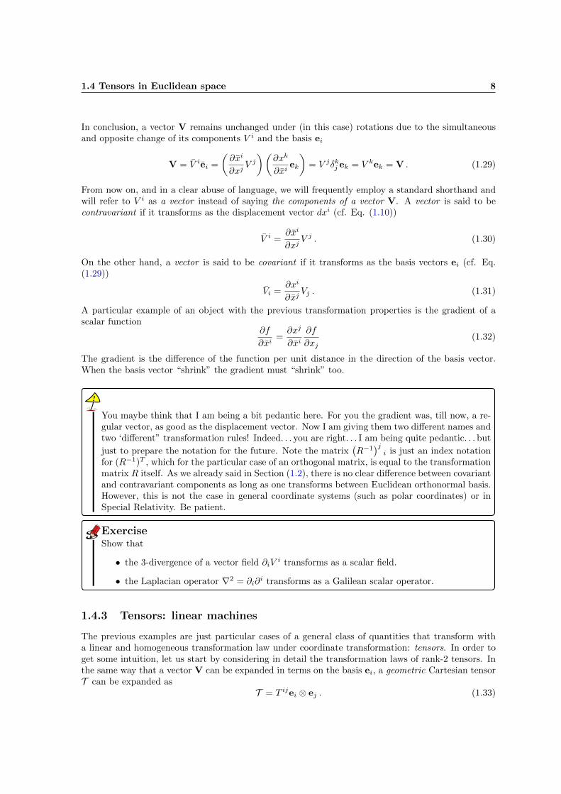
Rotations ∂xi

∂xj ≡ Rij are constants!

Scalar φ = φ

Contravariant vector V i = ∂xi

∂xj Vj

Covariant vector Vi = ∂xj

∂xi Vj

Contravariant rank-2 tensor T ij = ∂xi

∂xk∂xj

∂xl Tkl

Covariant rank-2 tensor Tij = ∂xk

∂xi∂xl

∂xj Tkl

Mixed rank-2 tensor T ij = ∂xi

∂xk∂xl

∂xj Tkl

Table 1.1

where ⊗ denotes the direct product. The transformation property of the different components T ij

under a rotation follows immediately from the previous expresion: T ij transform as the product oftwo contravariant vectors Ai and Bj

AiBj = RikR

jlA

kAl −→ T ij = RikR

jlT

kl . (1.34)

As we did in the previous section, we can define the covariant tensor Tij , which transform as theproduct of two covariant vectors

AiBj =(R−1

)ki

(R−1

)ljAkAl −→ Tij =

(R−1

)ki

(R−1

)ljTkl . (1.35)

As before, in a clear abuse of language, we will refer to these tensor components as tensors. Particularexamples of rank-2 Cartesian tensor are the inertia tensor

Iij =

∫d3x ρ(x)

(r2δij − xixj

)(1.36)

or the quadrupole tensor (1.57) (cf. Section 1.5.1).

ExerciseShow that the inertia tensor Iij is indeed a rank-(2,0) tensor.

Generalizing the transformation laws (1.34) and (1.35) we can define the transformations propertiesfor arbitrary mixed tensors of contravariant rank m and covariant rank n

T i1...imj1...jn =

(m∏

p=1

∂xip

∂xkp

n∏q=1

∂xlq

∂xjq

)T k1...km

l1...ln (1.37)

=[Ri1

k1 . . . Rim

km

] [(R−1)l1 j1 . . . (R

−1)ln jn

]T k1...km

l1...ln . (1.38)

Tensors (components) are objects with any number of indices. They share the same transformationproperties as vectors and can be classified according to the number of upper or lower indices. Forinstance, we say that a scalar is a rank-0 tensor and a contravariant (or covariant) vector is a con-travariant (or covariant) rank-1 tensor. In general, a tensor with m upper indices and n lower indicesis called a rank-(m,n) tensor.

1.4 Tensors in Euclidean space 10

A tensor is not just a quantity carrying indices. It is the transformation law what defines atensor (see below). Not all quantities with indices are tensors.

1.4.4 Some useful properties

Let me present some useful properties and definitions regarding tensors:

1. The sum (or difference) of two like-tensors is a tensor of the same kind. The proof of this isstraightforward. Imagine we take sum or difference of two general tensors T i1...im

j1...jn andRi1...im

j1...jn and apply the transformation rule (1.37), we will get

Si1...imj1...jn ≡ T i1...im

j1...jn ± Ri1...imj1...jn

=

(m∏

p=1

∂xip

∂xkp

n∏q=1

∂xlq

∂xjq

)T k1...km

l1...ln ±

(m∏

p=1

∂xip

∂xkp

n∏q=1

∂xlq

∂xjq

)Rk1...km

l1...ln

=

(m∏

p=1

∂xip

∂xkp

n∏q=1

∂xlq

∂xjq

)(T k1...km

l1...ln ±Rk1...kml1...ln

)=

(m∏

p=1

∂xip

∂xkp

n∏q=1

∂xlq

∂xjq

)Si1...im

j1...jn . (1.39)

2. Given two tensors of rank s and t, the product transforms as a tensor of rank (s+ t).

3. If the expression T ...... = R...

...S...

... is invariant under coordinate transformations and T ...... and

R...... are tensors, then S...

... is a tensor.

ExerciseProve this for the particular case Ti = RjS

ji.

4. A tensor contraction occurs when one of a tensor’s free covariant indices is set equal to oneof its free contravariant indices6. A sum is understood to be performed on the now repeatedindices. For instance, Tij

j is a contraction on the second and third indices of the tensor Tijk.

5. The contraction of a rank-2 tensor is a scalar (its trace) whose value is independent of thecoordinate system chosen.

If all the components of a Cartesian tensor T i1...imj1...jn in a given inertial reference frame are

zero, they will be zero in any other inertial reference frame.

6Note the words covariant and contravariant. A contraction is never done between two covariant or two contravariantindices.

1.4 Tensors in Euclidean space 11

1.4.5 Symmetric and antisymmetric tensors

An arbitrary rank-2 tensor can be decomposed into a completely symmetric and a completely anti-symmetric part

Tij = T(ij) + T[ij] , (1.40)

where we have used the common notation (, ) and [, ] to denote respectively symmetrization andantisymmetrization over the indices included inside, i.e.

T(ij) ≡1

2(Tij + Tji) , T[ij] ≡

1

2(Tij − Tji) . (1.41)

Completely symmetric and antisymmetric rank-2 tensors satisfy Tij = ±Tji, where the plus sign standsfor the symmetric and the minus sign for the antisymmetric one. Particular examples of symmetrictensors are the inertia tensor (1.36) or the quadrupole tensor (1.57) (cf. Section 1.5.1).

ExerciseProve that the trace of a tensor is invariant under rotations. Show that a tensor Tij in ndimensions has three separately invariant parts

Tij =1

nT k

kδij + T(ij) +

(T[ij] −

1

nT k

kδij

). (1.42)

ExerciseWrite down the explicit expressions for the completely symmetric and antisymmetric parts of arank-3 tensor Tijk.

1.4.6 Permutation tensor

The Levi-Civita or permutation tensor7 of rank 3

εijk = εijk

+1, if ijk is an even permutation of 123

+1, if ijk is an odd permutation of 123

0, otherwise

(1.43)

flips the sign upon the interchange of any pair of indices and vanishes when two of the indices areequal. Most of the basic identities of vector algebra and vector calculus can be easily proved by usingan important relation between the metric tensor δij and εijk, the contracted epsilon identity8

εijkεilm = δjlδkm − δjmδkl . (1.44)

You will deal with this expression in the exercises.

7Technically, I should say that it is a psedotensor, but we are not interested in introducing this concept here. Wewill only deal with rotations.

8In most of the books you will find this expression with all indices down. Remember that the index convention wechose is just a way of keeping track of the sums that can be easily extended to the Minkowski case. For Cartesiantensors the position of the indices makes no difference.

1.5 Covariance and Classical Mechanics 12

1.5 Covariance and Classical Mechanics

The main property of tensors is that their transformation law is linear and homogeneous. Eachcomponent of a tensor, in this case Cartesian, is a linear combination of the components of the tensorin the original frame, namely

T i1...imj1...jn =

(m∏

p=1

∂xip

∂xkp

n∏q=1

∂xlq

∂xjq

)T k1...km

l1...ln . (1.45)

In order to ensure that fundamental equations satisfy the Galilean Principle of Relativity the onlything we have to do is to write tensorial equations. For instance, if two quantities Sij

k and T ijk

transform as rank-(2, 1) Cartesian tensors, a fundamental law of the kind

Sijk = T ij

k , (1.46)

will retain its form in any inertial reference frame, since both sides of the equation transform in thesame way under coordinate transformations (in this case rotations). The fundamental equation (1.46)is then said to be covariant and the transformation is said to be a symmetry of the physical theory.

1.5.1 Newton’s theory of gravity

A physical example of the previous discussion is the Newtonian theory of gravity published by Netwonin 1687 within the Philosophiae Naturalis Principia Mathematica. In such a theory, the gravitationalforce Fi exerted on a gravitational test mass mG

Fi = −mG ∂iΦ . (1.47)

is determined by a single function9, the gravitational potential Φ, which depends on the matter dis-tribution through the so-called Poisson equation10

∇2Φ(t, xi) = 4πGρ(t, xi) . (1.49)

Eqs. (1.47) and (1.49) are respectively a vector and a scalar covariant equation. If they are valid ina given inertial frame, they will be automatically valid in any inertial frame, since their form will bepreserved under rotations and translations.

Exercise: Cosmological constantGalilean invariance allows for an additional constant Λ in the Poisson equation, which becomes

∇2Φ(t,x) + Λ = 4πGρ(t,x) . (1.50)

Observations of galaxies with typical masses of 1030M�, and intergalactic separations of order1 Mly do not show any significant deviation from Newton’s inverse square. law. Assuming thisdeviation to be smaller than 1%, determine an upper bound on the magnitude of Λ.

9Eqs. (1.47) and (1.49) are left unaltered by the addition to Φ of an arbitrary function of time f(t), namely

Φ(t,x)→ Φ(t,x) + f(t) . (1.48)

Since the transformation affects only the field Φ and not the coordinates, the invariance of Eqs. (1.47) and (1.49) under(1.48) is referred as an internal or gauge symmetry. The gravitational field Φ(t,x) has no dynamical degrees of freedom.Eq. (1.49) is not a dynamical equation for the determination of the potential, but rather a constraint on the initialspatial distribution of the potential, which must apply at all times.

10No value of the proportionality Newton’s gravitational constant G was available to Newton. Its numerical value wasfirstly determined by Cavendish in 1797 using a torsion balance, being the result reasonably close to present laboratorymeasurements, G = 6.673(10) × 10−11N m2/ kg2. The gravitational constant remains the most uncertain of all thefundamental constants of physics.

1.5 Covariance and Classical Mechanics 13

x'

x

x- x'

P

O

Figure 1.3: Multipolar expansion.

The solution of the Poisson equation can be worked out in the same way that you did for theelectromagnetic potential in your Classical Electrodynamics course. The only difference (albeit fun-damental) is the sign of the matter distribution. A formal solution of the Poisson’s equation for anarbitrary mass distribution can be obtained by applying the superposition principle or using Greenfunctions to obtain

Φ(x) = −G∫

ρ(x′)

|x− x ′|d3x′ , (1.51)

where x = xiei is the radius vector of the point at which the gravitational potential is computed,and x′ = x′iei is an arbitrary point in the matter distribution. Note that the Newtonian potential isnegative, as expected for an attractive force.

Exercise: Green’s functions (*)Use the Green’s function method to prove Eq.(1.51).

The previous expression becomes the usual −GM/r only for a spherical mass distribution. Thegeneral result for a non-spherical distribution is slightly more complicated. As any distribution func-tion, the essential features of the matter distribution can be be characterized by its moments. For anobserver sufficiently far away from the object we can perform a Taylor expansion around x′ = 0 toobtain

1

|x− x′|= e−x

′·∇ 1

r=

1

r− (x′ · ∇)

1

r+

1

2(x′ · ∇)2 1

r+ . . .+

(−1)n

n!(x′ · ∇)n

1

r+ . . . (1.52)

=1

r+x′kxkr3

+

(3x′kx′l − r′2δkl

)xkxl

2r5+ . . . , (1.53)

where we have used the standard expression for the exponential ex =∑∞

n=0(−1)n

n! xn and defined thedistance r2 = xkxk. Inserted back in Eq.(1.51), we realize that the potential created by the matterdistribution

Φ(x) = −G[M

r+Dkxkr3

+Qklxkxl

2r5+ . . .

], (1.54)

can be organized in a series whose individual terms contain information on the spatial structure at anincreasing level of detail while decaying the more rapidly in space the higher the information contentis. The quantities

M =

∫ρ(x′) d3x′ , (1.55)

Dk =

∫ρ(x′)x′kd3x′ , (1.56)

and

Qkl =

∫ρ(x′)

(3x′kx′l − r′2δkl

)d3x′ , (1.57)

1.5 Covariance and Classical Mechanics 14

are respectively the total mass of the system, the mass dipole moment and the mass quadrupole mo-ment tensor. The dipole moment can be eliminated by simply choosing the origin of coordinates ofthe center of mass. The quadrupole moment is the second moment of the mass distribution with itstrace removed. It is proportional to 1/r3, which gives rise to a deviation from the inverse square lawof the form 1/r4.

Exercise: Multipole expansion• Prove Eq. (1.52).

• Prove that the quadrupole tensor for a spherical distribution vanishes.

• Prove that a change of the origin modifies the quadrupole tensor by only adding a constant.