ETSI TR 103 257-1 V1.1.1 (2019-05)

Intelligent Transport Systems (ITS); Access Layer;

Part 1: Channel Models for the 5,9 GHz frequency band

TECHNICAL REPORT

ETSI

ETSI TR 103 257-1 V1.1.1 (2019-05)2

Reference DTR/ITS-00437-1

Keywords ITS, radio, V2X

ETSI

650 Route des Lucioles F-06921 Sophia Antipolis Cedex - FRANCE

Tel.: +33 4 92 94 42 00 Fax: +33 4 93 65 47 16

Siret N° 348 623 562 00017 - NAF 742 C

Association à but non lucratif enregistrée à la Sous-Préfecture de Grasse (06) N° 7803/88

Important notice

The present document can be downloaded from: http://www.etsi.org/standards-search

The present document may be made available in electronic versions and/or in print. The content of any electronic and/or print versions of the present document shall not be modified without the prior written authorization of ETSI. In case of any

existing or perceived difference in contents between such versions and/or in print, the prevailing version of an ETSI deliverable is the one made publicly available in PDF format at www.etsi.org/deliver.

Users of the present document should be aware that the document may be subject to revision or change of status. Information on the current status of this and other ETSI documents is available at

https://portal.etsi.org/TB/ETSIDeliverableStatus.aspx

If you find errors in the present document, please send your comment to one of the following services: https://portal.etsi.org/People/CommiteeSupportStaff.aspx

Copyright Notification

No part may be reproduced or utilized in any form or by any means, electronic or mechanical, including photocopying and microfilm except as authorized by written permission of ETSI.

The content of the PDF version shall not be modified without the written authorization of ETSI. The copyright and the foregoing restriction extend to reproduction in all media.

© ETSI 2019.

All rights reserved.

DECTTM, PLUGTESTSTM, UMTSTM and the ETSI logo are trademarks of ETSI registered for the benefit of its Members. 3GPPTM and LTETM are trademarks of ETSI registered for the benefit of its Members and

of the 3GPP Organizational Partners. oneM2M™ logo is a trademark of ETSI registered for the benefit of its Members and

of the oneM2M Partners. GSM® and the GSM logo are trademarks registered and owned by the GSM Association.

ETSI

ETSI TR 103 257-1 V1.1.1 (2019-05)3

Contents

Intellectual Property Rights ........................................................................................................................ 5

Foreword ..................................................................................................................................................... 5

Modal verbs terminology ............................................................................................................................ 5

1 Scope ................................................................................................................................................ 6

2 References ........................................................................................................................................ 6

2.1 Normative references ................................................................................................................................ 6

2.2 Informative references ............................................................................................................................... 6

3 Definition of terms, symbols and abbreviations ............................................................................... 8

3.1 Terms ......................................................................................................................................................... 8

3.2 Symbols ..................................................................................................................................................... 8

3.3 Abbreviations ............................................................................................................................................ 8

4 Introduction .................................................................................................................................... 10

4.1 Wave propagation.................................................................................................................................... 10

4.2 Common channel models ........................................................................................................................ 11

4.3 Usage of channel models ......................................................................................................................... 13

4.4 The 5,9 GHz frequency band and V2X communication ......................................................................... 13

4.5 Scenarios ................................................................................................................................................. 13

4.5.1 Introduction........................................................................................................................................ 13

4.5.2 Urban ................................................................................................................................................. 14

4.5.3 Rural .................................................................................................................................................. 15

4.5.4 Highway ............................................................................................................................................. 15

4.5.5 Tunnels .............................................................................................................................................. 15

4.5.6 LOS probability ................................................................................................................................. 16

4.6 Summary ................................................................................................................................................. 16

5 Channel models .............................................................................................................................. 16

5.1 Introduction ............................................................................................................................................. 16

5.2 Path loss models ...................................................................................................................................... 16

5.2.1 Free space path loss model ................................................................................................................ 16

5.2.2 Two-way ground reflection model ..................................................................................................... 17

5.2.3 Log-distance path loss model............................................................................................................. 18

5.3 Tapped delay line model ......................................................................................................................... 18

5.4 Geometry-based stochastic channel model .............................................................................................. 19

5.4.1 Introduction........................................................................................................................................ 19

5.4.2 General parameters ............................................................................................................................ 19

5.4.2.1 Introduction .................................................................................................................................. 19

5.4.2.2 Step 1 - Set scenario ..................................................................................................................... 20

5.4.2.3 Step 2 - LOS/NLOS/NLOSv ........................................................................................................ 20

5.4.2.4 Step 3 - Path loss and shadowing ................................................................................................. 21

5.4.2.4.1 Path loss models and vehicle blockage loss............................................................................ 21

5.4.2.4.2 Shadow fading ........................................................................................................................ 22

5.4.2.5 Step 4 - Large scale correlated scatterers ..................................................................................... 23

5.4.3 Small scale parameters ....................................................................................................................... 25

5.4.3.1 Introduction .................................................................................................................................. 25

5.4.3.2 Step 5 - Generate delays ............................................................................................................... 25

5.4.3.3 Step 6 - Generate cluster powers .................................................................................................. 26

5.4.3.4 Step 7 - Generate arrival and departure angles ............................................................................. 26

5.4.3.5 Step 8 - Perform random coupling of rays ................................................................................... 28

5.4.3.6 Step 9 - Generate XPRs ................................................................................................................ 28

5.4.4 Coefficient generation ........................................................................................................................ 28

5.4.4.1 Introduction .................................................................................................................................. 28

5.4.4.2 Step 10 - Draw initial random phases .......................................................................................... 29

5.4.4.3 Step 11 - Generate channel coefficients ....................................................................................... 29

5.4.4.4 Step 12 - Apply path loss and shadowing .................................................................................... 31

5.5 Channel Models for Link Level Simulations........................................................................................... 31

ETSI

ETSI TR 103 257-1 V1.1.1 (2019-05)4

5.5.1 Cluster Delay Line Models ................................................................................................................ 31

5.5.1.1 Introduction .................................................................................................................................. 31

5.5.1.2 CDL parameters for LLS ............................................................................................................. 32

5.5.2 Map-based hybrid channel model (Alternative channel model methodology) .................................. 34

5.5.2.1 Overview ...................................................................................................................................... 34

5.5.2.2 Coordinate system ........................................................................................................................ 34

5.5.2.3 Scenarios ...................................................................................................................................... 34

5.5.2.4 Antenna modelling ....................................................................................................................... 34

5.5.2.5 Channel generation....................................................................................................................... 35

5.5.2.5.1 Introduction ............................................................................................................................ 35

5.5.2.5.2 Step 1: Set environment and import digitized map ................................................................. 35

5.5.2.5.3 Step 2: Set network layout and antenna array parameters ...................................................... 35

5.5.2.5.4 Step 3: Apply ray-tracing to each pair .................................................................................... 36

5.5.2.5.5 Step 4: Generate large scale parameters ................................................................................. 37

5.5.2.5.6 Step 5: Generate delays for random clusters .......................................................................... 37

5.5.2.5.7 Step 6: Generate powers for random clusters ......................................................................... 38

5.5.2.5.8 Step 7: Generate arrival angles and departure angles ............................................................. 38

5.5.2.5.9 Step 8: Merge deterministic clusters and random clusters ...................................................... 39

5.5.2.5.10 Step 9: Generate ray delays and ray angle offsets .................................................................. 40

5.5.2.5.11 Step 10: Generate power of rays in each cluster ..................................................................... 41

5.5.2.5.12 Step 11: Generate XPRs ......................................................................................................... 41

5.5.2.5.13 Step 12: Draw initial random phases ...................................................................................... 41

5.5.2.5.14 Step 13: Generate channel coefficients ................................................................................... 41

Annex A: Mahler model for tracking multipath components .................................................... 44

Annex B: LOS probability and transition probability curves ................................................... 45

Annex C: Coordinate system ......................................................................................................... 48

C.1 Definition ....................................................................................................................................... 48

C.2 Local and global coordinate systems .............................................................................................. 48

C.3 Transformation from a LCS to a GCS ............................................................................................ 48

C.4 Transformation from an LCS to a GCS for downtilt angle only .................................................... 52

Annex D: Ensuring Spatial consistency in GBSCM models ....................................................... 54

Annex E: Bibliography .................................................................................................................. 57

History ...................................................................................................................................................... 59

ETSI

ETSI TR 103 257-1 V1.1.1 (2019-05)5

Intellectual Property Rights

Essential patents

IPRs essential or potentially essential to normative deliverables may have been declared to ETSI. The information pertaining to these essential IPRs, if any, is publicly available for ETSI members and non-members, and can be found in ETSI SR 000 314: "Intellectual Property Rights (IPRs); Essential, or potentially Essential, IPRs notified to ETSI in respect of ETSI standards", which is available from the ETSI Secretariat. Latest updates are available on the ETSI Web server (https://ipr.etsi.org/).

Pursuant to the ETSI IPR Policy, no investigation, including IPR searches, has been carried out by ETSI. No guarantee can be given as to the existence of other IPRs not referenced in ETSI SR 000 314 (or the updates on the ETSI Web server) which are, or may be, or may become, essential to the present document.

Trademarks

The present document may include trademarks and/or tradenames which are asserted and/or registered by their owners. ETSI claims no ownership of these except for any which are indicated as being the property of ETSI, and conveys no right to use or reproduce any trademark and/or tradename. Mention of those trademarks in the present document does not constitute an endorsement by ETSI of products, services or organizations associated with those trademarks.

Foreword This Technical Report (TR) has been produced by ETSI Technical Committee Intelligent Transport Systems (ITS).

Modal verbs terminology In the present document "should", "should not", "may", "need not", "will", "will not", "can" and "cannot" are to be interpreted as described in clause 3.2 of the ETSI Drafting Rules (Verbal forms for the expression of provisions).

"must" and "must not" are NOT allowed in ETSI deliverables except when used in direct citation.

ETSI

ETSI TR 103 257-1 V1.1.1 (2019-05)6

1 Scope The present document provides a set of channel models describing how signals in the 5,9 GHz frequency band are perturbed by the mobile radio environment in different use cases.

2 References

2.1 Normative references Normative references are not applicable in the present document.

2.2 Informative references References are either specific (identified by date of publication and/or edition number or version number) or non-specific. For specific references, only the cited version applies. For non-specific references, the latest version of the referenced document (including any amendments) applies.

NOTE: While any hyperlinks included in this clause were valid at the time of publication, ETSI cannot guarantee their long term validity.

The following referenced documents are not necessary for the application of the present document but they assist the user with regard to a particular subject area.

[i.1] I. Tan, W. Tang, K. Labertaux and A. Bahai: "Measurement and analysis of wireless channel impairments in DSRC vehicular communications", in Proc. Of International Conference on Communications (ICC '08), Beijing, China, May 2008, pp. 4882-4888. .

[i.2] P. Alexander, D. Haley, and A. Grant: "Cooperative intelligent transport systems: 5.9 GHz field trials", in Proceedings of the IEEE, vol. 99, no. 7, pp. 1213-1235, July 2011. .

[i.3] L. Bernado, T. Zemen, F. Tufvesson, A. F. Molisch and C. F. Mecklenbräuker: "Delay and Doppler spreads of non-stationary vehicular channels for safety relevant scenarios", in IEEE Transactions on Vehicular Technology, vol. 63, no. 1, pp. 82-93, January 2014. .

[i.4] T. S. Rappaport, Wireless Communications: "Principles and Practice", Prentice Hall, 1996.

[i.5] M. Boban, J. Barros and O. Tonguz: "Geometry-based vehicle-to-vehicle channel modeling for large-scale simulation", in IEEE Transactions on Vehicular Technology, vol. 63. No. 9, pp. 4146-4164, November 2014.

[i.6] M. Boban, T. T. V. Vinhoza, M. Ferreira, J. Barros and O. K. Tonguz: "Impact of vehicles as obstacles in vehicular ad hoc networks", in IEEE Journal on Selected Areas in Communications, vol. 29, no. 1, pp. 15-28, January 2011.

[i.7] K. Mahler, W. Keusgen, F. Tufvesson, T. Zemen and G. Caire: "Measurement-Based Wideband Analysis of Dynamic Multipath Propagation in Vehicular Communication Scenarios", in IEEE Transactions on Vehicular Technology, October 2016.

[i.8] M. Boban, W. Viriyasitavat and O.K. Tonguz: "Modeling vehicle-to-vehicle line of sight channels and its impact on application-layer performance", in Proceeding of the 10th ACM international workshop on Vehicular inter-networking, systems, and applications (VANET 13), Taipei, Taiwan, June 2013, pp. 91-94. .

[i.9] J. Karedal, N. Czink, A. Paier, F. Tufvesson and A. Molisch: "Path loss modelling for vehicle-to-vehicle communications", in IEEE Transactions on Vehicular Technology, vol. 60, no. 1, pp. 323-328, January 2011.

[i.10] Recommendation ITU-R P.526: "Propagation by diffraction", International Telecommunication Union Radiocommunication Sector, Geneva, November 2013. .

ETSI

ETSI TR 103 257-1 V1.1.1 (2019-05)7

[i.11] M. Boban, X. Gong and W. Xu: "Modeling the evolution of line-of-sight blockage for V2V channels", in Proceedings of the 2016 IEEE 84th Vehicular Technology Conference (VTC2016-Fall), Montréal, Canada, September 2016, pp. 1-6.

[i.12] ETSI TR 102 638 (V1.1.1) (2009-06): "Intelligent Transport Systems (ITS); Vehicular Communications; Basic Set of Applications; Definitions".

[i.13] ETSI TR 138 901 (V14.0.0) (2017-03): "5G; Study on channel model for frequencies from 0.5 to 100 GHz (3GPP TR 38.901 version 14.0.0 Release 14)".

[i.14] B. Aygun, M. Boban, J.P. Vilela and A.M. Wyglinski: "Geometry-Based Propagation Modeling and Simulation of Vehicle-to-Infrastructure Links", in Proceedings of the 2017 IEEE 83th Vehicular Technology Conference (VTC2016-Spring), Nanjing, China, May 2016, pp. 1-5.

[i.15] T. Mangel, O. Klemp and H. Hartenstein: "5.9 GHz inter-vehicle communication at intersections: a validated non-line-of-sight path-loss and fading model", in EURASIP Journal on Wireless Communications and Networking 2011, 2011:182 DOI: 10.1186/1687-1499-2011-182.

[i.16] WINNER Project Board: "D5.4 v1.4 - Final Report on Link Level and System Level Channel Models", 18 November 2005.

NOTE: Available at https://www.researchgate.net/publication/229031750_IST-2003-507581_WINNER_D5_4_v_14_Final_Report_on_Link_Level_and_System_Level_Channel_Models.

[i.17] WINNER Project Board: "D1.1.2 V1.2 - WINNER II Channel Models", 30 09 2007.

NOTE: Available at https://www.cept.org/files/8339/winner2%20-%20final%20report.pdf.

[i.18] WINNER Project Board: "D5.3 - WINNER+ Final Channel Models", 30 06 2010.

NOTE: Available at https://www.researchgate.net/publication/261467821_CP5-026_WINNER_D53_v10_WINNER_Final_Channel_Models.

[i.19] 3GPP TR 37.885 (2018-05): "Study on evaluation methodology of new Vehicle-to-Everything V2X use cases for LTE and NR".

[i.20] 3GPP TR 36.885: "Study on LTE-based V2X services".

[i.21] L. Liu, C. Oestges, J. Poutanen, K. Haneda, P. Vainikainen, F. Quitin and P. De Doncker: "The COST 2100 MIMO channel model", in IEEE Wireless Communications, vol. 19, no. 6, pp. 92-99, December 2012.

[i.22] RESCUE project deliverable D4.3: "Report on channel analysis and modeling".

NOTE: Available at https://cordis.europa.eu/docs/projects/cnect/5/619555/080/deliverables/001-D43v10FINAL.pdf.

[i.23] M. Walter, D. Shutin and U.-C. Fiebig: "Delay-Dependent Doppler Probability Density Functions for Vehicle-to-Vehicle Scatter Channels", in IEEE Transactions on Antennas and Propagation, vol. 62, no. 4, pp. 2238-2249, April 2014.

[i.24] M. Walter, T. Zemen and D. Shutin: "Empirical relationship between local scattering function and joint probability density function", 2015 IEEE 26th Annual International Symposium on Personal, Indoor, and Mobile Radio Communications (PIMRC), Hong Kong, 2015, pp. 542-546.

[i.25] H. Friis: "A note on a simple transmission formula", in Proceedings of the IRE, vol. 34, no. 5, pp. 254-256, May 1946.

[i.26] Glassner, A S: "An introduction to ray tracing", Elsevier, 1989.

[i.27] R.G. Kouyoumjian and P.H. Pathak: "A uniform geometrical theory of diffraction for an edge in a perfectly conducting surface", in Proceedings of IEEE, vol. 62, no. 11, pp. 1448-1461, November 1974.

ETSI

ETSI TR 103 257-1 V1.1.1 (2019-05)8

[i.28] P. H. Pathak, W. Burnside and R. Marhefka: "A Uniform GTD Analysis of the Diffraction of Electromagnetic Waves by a Smooth Convex Surface", in IEEE Transactions on Antennas and Propagation, vol. 28, no. 5, pp. 631-642, 1980.

[i.29] J. W. McKown, R. L. Hamilton: "Ray tracing as a design tool for radio networks", in IEEE Network, vol. 5, no. 6, pp. 27-30, November 1991.

[i.30] ICT-317669-METIS/D1.4: "METIS channel model", METIS 2020, February 2015.

[i.31] W. Tomasi: "Electronic Communication Systems - Fundamentals Through Advanced", Pearson. pp. 1023.

[i.32] J. Deygout: "Multiple knife-edge diffraction of microwaves", in IEEE Transactions on Antennas and Propagation, vol. 14, no. 4, 1966, pp .480-489.

3 Definition of terms, symbols and abbreviations

3.1 Terms Void.

3.2 Symbols For the purposes of the present document, the following symbols apply:

GRX Antenna Gain Receiver GTX Antenna Gain Transmitter KR Ricean K factor LRC parameter denoting the number of random clusters LRT parameter denoting the number of deterministic clusters

3.3 Abbreviations For the purposes of the present document, the following abbreviations apply:

AOA Angle of Arrival AOD Angle of Departure B2R Base station to road side unit C-ITS Cooperative ITS DUT Device Under Test ITS Intelligent Transport Systems LOS Line-Of-Sight LSP Large-Scale-Parameters MAC Medium Access Control MD Mobile Discrete MPC MultiPath Component NGSM Non-Geometry Stochastic Model NLOS Non-LOS caused by objects other than vehicles NLOSv Non-LOS caused by vehicles P2B Pedestrian to base station P2P Pedestrian to pedestrian PAS Power angular spread PDF Probability Density Function PL Path Loss R2R Road side unit to road side unit RMS Root Mean Squared RSU Road side unit RX Receiver

ETSI

ETSI TR 103 257-1 V1.1.1 (2019-05)9

SD Static Discrete SF Shadow Fading TDL Tapped Delay Line TX Transmitter US Uncorrelated Scatterers V2B Vehicle to base station V2I Vehicle-to-Infrastructure V2P Vehicle to pedestrian V2V Vehicle-to-Vehicle V2R Vehicle to road side unit V2X Vehicle-to-X VANET Vehicular ad hoc networks WSS Wide Sense Stationary XPR Cross Polarization power Ratios ZOA Zenith angles Of Arrival ZOD Zenith angles Of Departure ZSD Zenith angle Spreads at Departure GBDM Geometry-based deterministic model NS Network Simulator PHY Physical Layer FSPL Free Space Path Loss GBSCM Geometry-based stochastic channel model SLS System Level Simulations LLS Link Level Simulations DS Delay Spread ASA Azimuth angle Spread of Arrival ASD Azimuth angle Spread of Departure ZSA Zenith angle Spread of Arrival FIR Finite Impuls Response BS-UT Base Station-User Terminal GCS Global Coordinate System CDL Cluster Delay Line SCM Stochastic Channel Model NR New Radio UTD Uniform Theory of Diffraction TOA Time Of Arrival BS Base Station UT User Terminal LCS Local Coordinate System PDP Probability Density Plot WIM WINNER Channel Model WIM-SC WIM-Spatial Consistency

ETSI

ETSI TR 103 257-1 V1.1.1 (2019-05)10

4 Introduction

4.1 Wave propagation Channel models, also called propagation models, are an important part when designing and evaluating wireless systems from the reception at the antenna all way up to the end user application. Channel models aim at mimic the perturbation signals undergo when travelling between transmitter (TX) and receiver (RX). The different effects that can be seen in a wireless channel are attenuation, reflection, transmission, diffraction, scattering, and wave guiding. The signal strength is decaying as the distance increases between TX and RX, i.e. the signal gets attenuated. Wave guiding is an effect that actually preserves the signal strength due to the fact that the signal is restricted in its expansion. It can occur for example in urban canyons and tunnels. In Figure 1, reflection, transmission, scattering, and diffraction, are illustrated. Reflection occurs on smooth surfaces, whereas transmission is when the signal penetrates the object. Scattering spreads the signal in several directions, which occurs on rough surfaces, and diffraction is when the signal is bending around a sharp edge. Smooth, rough, large, and small, are all relative to the wavelength in question. Increased carrier frequency implies smaller wavelength (e.g. 5,9 GHz is equal to a wavelength of 5 cm), more optical propagation, smaller antennas, and higher attenuation (the signal strength is decaying faster with distance).

Figure 1: Different effects on the signal: transmission, reflection, scattering and diffraction

In wireless channels several replicas of the same signal can reach RX, which have bounced off different objects during propagation; and if TX and/or RX are moving there will be Doppler effects. This is relative movement of the TX/RX that shifts the frequency of the signal and makes it different at the receiver from the one that was originally transmitted. Figure 2 provides an example where RX receives one line-of-sight (LOS) component and two replicas of the signal that have bounced off objects (a multipath scenario).

Reflection

Transmission

Scattering

Diffraction

ETSI

ETSI TR 103 257-1 V1.1.1 (2019-05)11

Figure 2: Multipath scenario, where several replicas of the signal besides the LOS component reach RX

The multipath components (MPC) will travel longer distances and will therefore arrive later than the LOS component. These delayed copies of the signal give rise to self-interference at RX, which could be constructive or destructive, see Figure 3. The worst case of destructive interference is when two equally strong signals are shifted 180 degrees (see Figure 3(b)).

Figure 3: Constructive (a) and destructive self-interference (b)

4.2 Common channel models There is a diverse set of channel models, which increase in complexity when more details about the propagation environment are added. The simplest channel models are deterministic path loss models, where the attenuation of the signal is based on a predetermined formula using the carrier frequency and distance between TX and RX as input. In other words, this kind of models will always result in the same result when the frequency and the distance is the same. Two well-known path loss models are the free-space path loss model and the two-ray ground reflection model. Free-space only assumes a LOS component, whereas the two-ray ground reflection model is consisting of one LOS component and one ground reflection (one MPC). There exist more advanced path loss models where parameters are derived from real-world channel measurements for the LOS as well as for the situation when the LOS is blocked by another vehicle or building.

A path loss model is always present regardless of how complex the channel model is, since this deterministically decides the signal strength based on TX-RX separation, carrier frequency, and possible obstruction of LOS component. Path loss models suitable for V2X communication are further detailed in clause 5.2.

Statistical models add a fading component to the path loss model. Fading is the fluctuation of the signal strength and it is often modelled as a random process. Fading could either be due to multipath propagation (a.k.a. small-scale fading) or shadowing from obstacles affecting the propagation (a.k.a. large-scale fading). Small-scale fading is due to multipath propagation effect as mentioned earlier (see Figure 2) and gives rise to a certain amount of either constructive or destructive self-interference (see Figure 3). If there is a LOS component, this is usually very dominant since this contains the most energy compared to other copies of the signal (MPCs). Large-scale fading captures fluctuations on a larger scale above 10 wavelengths as opposed to small-scale fading, which is within a wavelength.

Building Building

TX RX

Line-of-sight

MPCs

MPC = Multipath component

+ = + =

(a) Constructive interference (b) Destructive interference

ETSI

ETSI TR 103 257-1 V1.1.1 (2019-05)12

Well-known statistical models for small-scale fading are Rayleigh, Rician, and Nakagami. In short, Rician distribution is used when the communication contains a LOS component and Rayleigh in absence of LOS. Nakagami captures both when there is a LOS and when this is absent. Nakagami is often used for protocol simulations of vehicular networks. Large-scale fading (shadowing) is very often represented by a Gaussian process.

In tapped delay line (TDL) models, individual MPCs are treated separately. Each MPC ("tap") will have its own fading statistics (e.g. Rician, Rayleigh) and phase shift, to cover phase differences between MPCs. Each tap may feature an individual Doppler spectrum. TDLs add better accuracy to the channel model by treating arriving MPC individually compared to when only using for example a Rician fading model (which could be regarded as only one signal hitting the RX). However, TDLs do not address the specific environment surrounding the vehicle such as buildings or objects that appear in different scenarios (however, a TDL could be tailored to a specific scenario).

TDLs and statistical models belong to the group of channel models that is called non-geometry based stochastic channel models (NGSM), which describe the paths between TX and RX by only statistical parameters without reference to the geometry.

Geometry-based stochastic channel models (GBSCM), on the other hand, also account for the environment such as buildings and vehicles, which are denoted scatterers. The geometry of the propagation environment is randomly generated according to specified statistical distributions. Dedicated vehicular radio channel measurements at 5 GHz show that the main contributions to the signal reception are LOS, deterministic scattering, and diffuse scattering components. The LOS component has high gain as long as there is a direct path from TX to RX. The LOS component's gain decreases whenever an interacting object obstructs the direct path (shadowing). The diffuse scattering contribution, stemming from surrounding buildings, other structures along the road, or foliage, forms a fairly large fraction of the overall channel gain.

Geometry-based deterministic model (GBDM) uses pure ray tracing or ray launching to determine the channel's characteristics. It needs 2.5D or 3D building data to search for all possible paths from TX to RX to find transmissions, reflections, diffraction, and scattering objects. Its result is deterministic. Searching for propagation paths is complex and it is computationally expensive. The complexity increases dramatically with the order of transmission and reflection, i.e. the number of possible interactions with objects. With increasing frequency band (decreasing wave length) the accuracy and hence reliability of ray tracing or launching based models decrease since impacts from material parameterization and small object detail modelling becomes more pronounced. Therefore, it is not a good choice to use it for a general channel model. Anyway, its deterministic approach can be used to create/parameterize new channel models as an alternative to time consuming real-world measurement campaigns. However, ray tracing allows for investigation of critical situations in which a statistical approach is not sufficient.

Table 1 summarizes the mentioned channel models and what aspects of the channel impairments each class of models try to address.

Table 1: Summary and description of different channel models

Channel model Path loss Fading Doppler Environment Description

Path loss X

Path loss models are integral in all channel models describing the deterministic signal attenuation based on TX-RX distance and carrier frequency.

Statistical models X X Adds a fading component (both small-scale and large-scale) to the path loss. Models only one received signal component.

TDL X X X Models several MPCs individually using statistics but can also add Doppler effects due to speed differences between TX and RX.

Geometry-based stochastic models

X X X X

Addresses also the environment by modelling potential scatterers according to statistical distributions which affect MPCs. Further, it addresses also the temporal evolution of the channel and thus considers correlations in time and space.

Geometry-based deterministic models

X X X X

Addresses the whole propagation environment in a deterministic way by generating each MPC and its interaction with the environment (including for example material of buildings, street signs, foliage, etc.). Very scenario specific and computational expensive.

ETSI

ETSI TR 103 257-1 V1.1.1 (2019-05)13

4.3 Usage of channel models A channel model is selected based on what part of the communication system that is going to be studied. For network level simulations, where communication protocols including medium access control (MAC) are studied, a statistical model (e.g. Rician, Rayleigh, and Nakagami) is the predominant channel model type to keep computational time down. These simulations usually consist of many vehicles to stress the network and protocols and to find weaknesses of the system as a whole. Well-known network simulators for vehicular ad hoc networks (VANET) are NS-2, NS-3, Veins, OMNET++, and OPNET. Statistical channel models found in the literature for VANETs are parameterized for specific scenarios such as urban and highway.

For physical (PHY) layer simulations more details about the channel is necessary to understand how a certain PHY is affected by for example delay and Doppler spreads due to multipath propagation. More details about the scenario itself needs to be present in PHY layer simulations. TDLs and geometry-based stochastic and deterministic channel models are for obvious reasons the preferred channel models for this kind of simulations.

4.4 The 5,9 GHz frequency band and V2X communication The 5,9 GHz band is a challenging frequency band for vehicle-to-vehicle (V2V) and vehicle-to-infrastructure (V2I) communications, collectively known as V2X communication, due to the high carrier frequency resulting in a wavelength of 5 cm. This frequency band provides a rich multipath environment especially in urban areas (many MPCs will arrive at RX). The LOS will often be blocked by other vehicles or buildings since the antennas are approximately on the same height especially in the V2V case. This results in many scatterers (both static and mobile) affecting the wave propagation especially in urban scenarios. Further, in highway scenarios high relative speeds can be achieved resulting in high Doppler. For communication with smart infrastructure (V2I), one node might be stationary and the antenna might be elevated resulting in a slightly better reception environment for moving vehicles but this is totally dependent on what kind of smart infrastructure that has been V2X enabled. The propagation channel for V2X is difficult to resemble due to the rich multipath environment.

4.5 Scenarios

4.5.1 Introduction

The selected V2X scenario has a major impact on the wave propagation and thus the channel model. There are three major scenarios: urban, rural, and highway, with the special case of tunnels. As the vehicle density increases in the different scenarios, the probability for the blockage of the LOS component increases and then strong MPCs needs to contribute to a successful reception of a transmission. Good reflectors are street signs and scatterers that are made of metallic structures with a smooth surface. However, good reflectors that are too far away can also cause a large delay spread resulting in inter-symbol interference and decoding problems when LOS is blocked. Delay spread is the delay between the first signal component arriving at the receiver and the last for a given symbol that is transmitted. Higher vehicle speeds can result in Doppler effect. In Figure 4, the scenarios detailed in subsequent clauses are illustrated.

Figure 4: V2X scenarios

ETSI

ETSI TR 103 257-1 V1.1.1 (2019-05)14

4.5.2 Urban

The urban scenario is defined as single-lane or multi-lane city streets used either for one-way or for two-way traffic in densely populated areas. There can be road signs, streetlights, traffic signs and traffic signals, single- to multi-story buildings situated along the roadsides and a multitude of traffic. The propagation channel in such a scenario is considered to have a rich scattering environment since there are many objects (both static as well as mobile) affecting the wave propagation and the antennas are situated at almost the same height close to the ground. The urban scenario will have a higher probability for blockage of the LOS component. Thus the successful reception of transmissions is based on strong MPCs. The Doppler effect will be small or zero since vehicles move with modest speeds in this scenario.

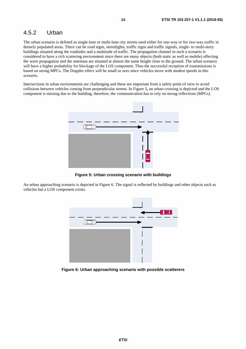
Intersections in urban environments are challenging and these are important from a safety point of view to avoid collisions between vehicles coming from perpendicular streets. In Figure 5, an urban crossing is depicted and the LOS component is missing due to the building, therefore, the communication has to rely on strong reflections (MPCs).

Figure 5: Urban crossing scenario with buildings

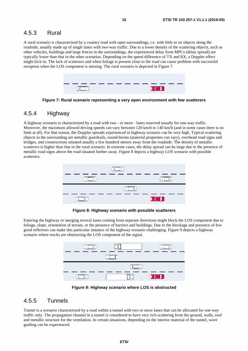
An urban approaching scenario is depicted in Figure 6. The signal is reflected by buildings and other objects such as vehicles but a LOS component exists.

Figure 6: Urban approaching scenario with possible scatterers

ETSI

ETSI TR 103 257-1 V1.1.1 (2019-05)15

4.5.3 Rural

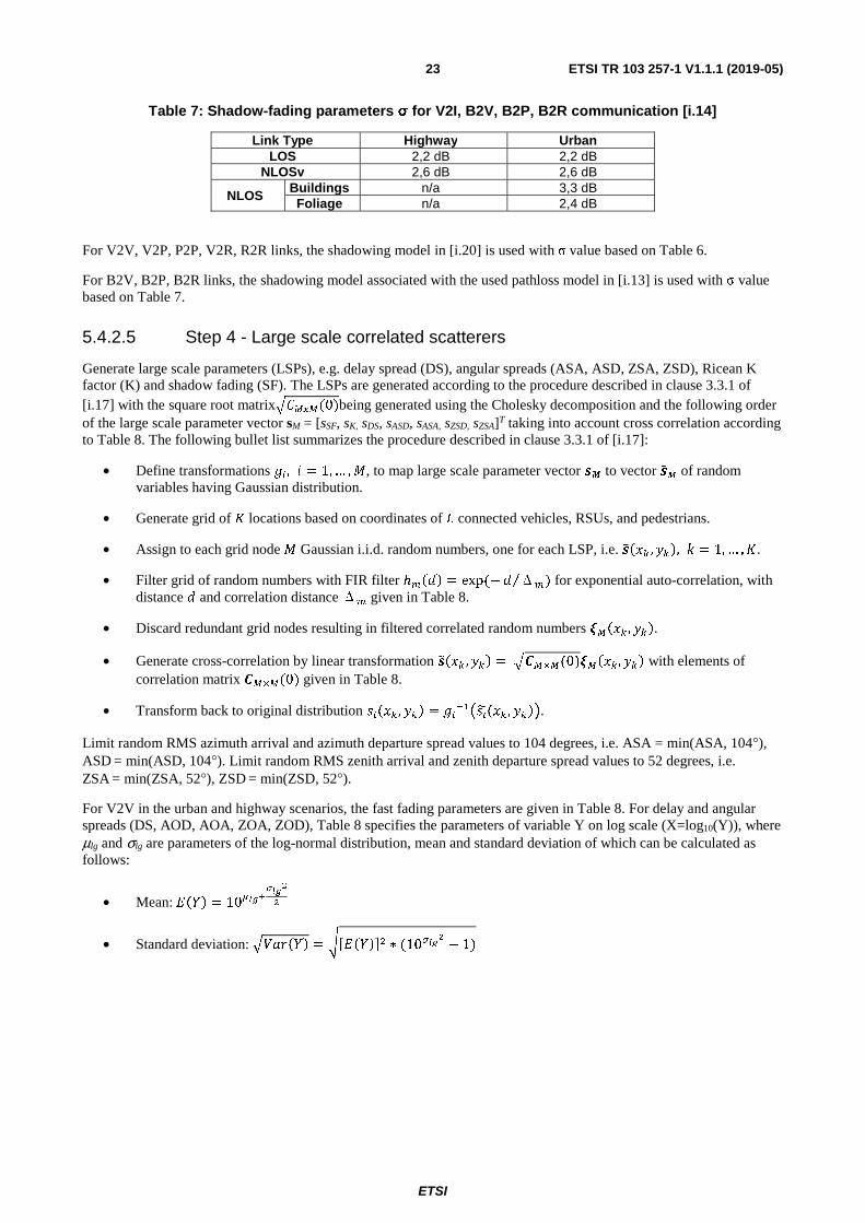
A rural scenario is characterized by a country road with open surroundings, i.e. with little to no objects along the roadside, usually made up of single lanes with two-way traffic. Due to a lower density of the scattering objects, such as other vehicles, buildings and large fences in the surroundings, the experienced delay from MPCs (delay spread) are typically lower than that in the other scenarios. Depending on the speed difference of TX and RX, a Doppler effect might kick-in. The lack of scatterers and when foliage is present close to the road can cause problem with successful reception when the LOS component is missing. The rural scenario is depicted in Figure 7.

Figure 7: Rural scenario representing a very open environment with few scatterers

4.5.4 Highway

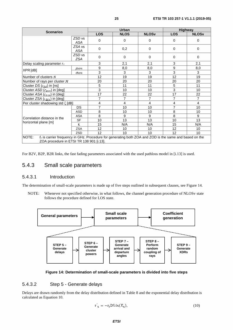
A highway scenario is characterized by a road with two - or more - lanes reserved usually for one-way traffic. Moreover, the maximum allowed driving speeds can vary between 120 km/h to 140 km/h (and in some cases there is no limit at all). For that reason, the Doppler spreads experienced in highway scenario can be very high. Typical scattering objects in the surrounding are metallic guardrails, sound-berms (material properties can vary), overhead road signs and bridges, and constructions situated usually a few hundred meters away from the roadside. The density of metallic scatterers is higher than that in the rural scenario. In extreme cases, the delay spread can be large due to the presence of metallic road signs above the road situated further away. Figure 8 depicts a highway LOS scenario with possible scatterers.

Figure 8: Highway scenario with possible scatterers

Entering the highway or merging several lanes coming from separate directions might block the LOS component due to foliage, slope, orientation of terrain, or the presence of barriers and buildings. Due to the blockage and presence of few good reflectors can make this particular instance of the highway scenario challenging. Figure 9 depicts a highway scenario where trucks are obstructing the LOS component of the signal.

Figure 9: Highway scenario where LOS is obstructed

4.5.5 Tunnels

Tunnel is a scenario characterized by a road within a tunnel with two or more lanes that can be allocated for one-way traffic only. The propagation channel in a tunnel is considered to have very rich scattering from the ground, walls, roof and metallic structure for the ventilation. In certain situations, depending on the interior material of the tunnel, wave guiding can be experienced.

ETSI

ETSI TR 103 257-1 V1.1.1 (2019-05)16

4.5.6 LOS probability

The blockage of the LOS component can be modelled statistically over time and space for V2V. When a blockage of LOS occurs between a specific TX-RX pair, this blockage might be persistent causing communication failures depending on the scenario. Realistic LOS blockage realization facilitates an appropriate parameter setting of path loss, small-scale, as well as large-scale fading parameters over time and space. Another way of finding the LOS blockage might be to look into every TX-RX pair in a mobility model and determine whether the communication between a specific TX-RX pair has LOS blockage or not and after that apply correct parameter setting for path loss and fading. Depending on the simulation scenario and the number of vehicles, the latter can quickly be very computational expensive and then a statistical model is preferred. In Annex B, more information about LOS probabilities is provided.

4.6 Summary Channel models for V2X communication are very complex due to the high carrier frequency resulting in a multipath propagation environment and road traffic safety/efficiency applications are very diverse in their nature, where the majority of applications are of broadcast nature (one transmission can be interesting to several recipients). This adds complexity when evaluating the system as a whole and since vehicles are moving everything depends on time and space. Scenarios need to be specific since small details determine the outcome of a possible simulation but too details will add unnecessary complexity. It is a balancing act to find the right channel model for supposed simulation scenario.

5 Channel models

5.1 Introduction This clause provides specific parameter settings for four different types of channel models:

1) deterministic path loss models;

2) statistical models;

3) tapped delay line models; and

4) geometry-based stochastic model.

5.2 Path loss models

5.2.1 Free space path loss model

The free space path loss model is the resulting loss in signal strength when the electromagnetic wave traverses from TX to RX through free space, without any obstacles nearby that could cause reflections or diffractions. The free space path loss FSPL is given by Equation 1.

(1)

where d is the distance between the transmitter and receiver, f is the carrier frequency, GTX and GRX is the gain of the transmitting and receiving antenna, respectively. Free space is a theoretical model which by itself does not model well the path loss for V2X channels since, at the very least, there are perturbations of the free space signal by the reflections coming from the road on which the vehicles travel.

ETSI

ETSI TR 103 257-1 V1.1.1 (2019-05)17

5.2.2 Two-way ground reflection model

The free space propagation model assumes the existence of only the LOS ray. However, due to the inherent structure of the environment where V2V communication occurs - over the face of road surface - in case of LOS communication the propagation characteristics are most often influenced by at least two dominant rays: LOS ray and ground-reflected ray. Two-way ground reflection model with appropriately adjusted reflection coefficient was shown as a very good path loss model for LOS V2V channels [i.8], [i.9]. It is based on a single street with one TX and one RX, neglecting obstacles. In this scenario, the LOS path interferes with the ground reflected path. The two rays arrive at the receiver with a different phase and a different power.

Figure 10: The two-ray ground reflection model

The different phase leads to constructive and destructive interference depending on the distance, dlos, between the receiver and the transmitter, as shown in Figure 10. When increasing the distance between the transmitter and the receiver, the alternating pattern of constructive and destructive interference stops at break point, db. From this distance onwards, the length difference between the two rays is smaller than half the wavelength and the small angle of arrival (AoA) on the ground causes a phase shift of 180° for the reflected wave, leading to destructive interference.

For these two rays and referring to Figure 10, the resulting E-field is equal to [i.8] and outlined in Equation 2.

E��� = E��� + E���� = ������

cos �ω� �t −������ + R����

�������

cos �ω� �t −����

��� (2)

where Eground is the E-field of the ground-reflected ray, Rground is the ground reflection coefficient, and dground is the propagation distance of the ground-reflected ray, where ht and hr is the height of the transmitting and receiving antenna, respectively, and dlos is the ground distance between the antennas see Figure 10. The parameter is defined in Equation 3:

� ����� = ��ℎ�� + ℎ�

�+ ����� ��

��� �

����� ��� (3)

Note that using the exact height of the antennas (ht and hr) is important, since a small difference in terms of either ht or hr results in significantly different interference relationship between the LOS and ground-reflected ray. When the originating medium is free space, the reflection coefficient R is calculated as follows for vertical and horizontal polarization respectively (see Chapter 4.6 in [i.4]). See Equation 4 and Equation 5.

R|| =� ��

�� ��� ��

����� ����

�� ��� ��

����� �� (4)

and

R⟘ =�� ��� ��

����� ���� ��� ��

����� �� (5)

where �i is the incident angle, and ϵr is the relative permittivity of the material. From E-fields in Equation 2, the ensuing received power Pr (in watts) is calculated as outlined in Equation 6 (assuming unit antenna gain at the receiver).

P� =|����|�!�

"#$ (6)

where λ is the wavelength and η is the intrinsic impedance (η = 120πohms in free space). Appropriate reflection coefficient needs to be used to match the measurements. To that end, in [i.8] curve fitting of the above model to measurement data yielded a ϵr value of 1,003 as the best fit (note that remaining parameters in the calculation of reflection coefficient are dependent on geometry only).

dlos

ETSI

ETSI TR 103 257-1 V1.1.1 (2019-05)18

5.2.3 Log-distance path loss model

Log-distance path loss is an extension of the free space path loss, where the path loss exponent does not necessarily equal two (as is the case in free space propagation), but is a function of the environment surrounding TX and RX.

Log-distance path loss model is formally expressed as outlined in Equation 7.

PL(d) = PL(d0) + 10γlog(d/d0) + Xσ (7)

where PL is the total path loss measured in decibel (dB), PL(d0) is the path loss at the reference distance d0, d is the distance between TX and RX, γ is the path loss exponent and Xσ describes the random shadowing effects. Finally, in Equation 8 the received power Pr is calculated.

Pr = Pt + Gt + Gr - PL(d) (8)

where Pt is the transmit power and Gt and Gr are antenna gains in dBi. Log-distance path loss with appropriate path loss exponent and shadowing deviation was experimentally shown to model well the path loss for V2V links in non-LOS cases but only for a limited set of scenarios [i.9], [i.5]. For V2V links at 5,9 GHz, the following values can be used [i.5]:

• d0 = 1 meter,

• PL(d0) = 47,8649,

• γ = 2,5 (slight obstruction by building),

• γ = 3 (strong obstruction by building).

Log-distance path loss is a simple model that requires as inputs a minimum number of parameters. If additional information about the environment and geometric relationships of the objects in environment, more complex models, ones that take into account specifics of the environment, can be employed. One such model was developed by Mangel et. al in [i.15] for NLOS path loss in the 5,9 GHz band and more details can be found in Annex A.

5.3 Tapped delay line model The tapped delay line models outlined in present clause are derived from the following [i.1], [i.2] and [i.3].

In Table 2, TDL models for several scenarios are provided.

Table 2: TDL models for a set of scenarios

Power [dB] Delay [ns] Doppler [Hz] Profile

Urban approaching LOS

Tap 1 0 0 0 Static Tap 2 -8 117 236 HalfBT Tap 3 -10 183 -157 HalfBT Tap 4 -15 333 492 HalfBT

Urban crossing NLOS

Tap 1 0 0 0 Static Tap 2 -3 267 295 HalfBT Tap 3 -4 400 -98 HalfBT Tap 4 -10 533 591 HalfBT

Rural LOS Tap 1 0 0 0 Static Tap 2 -14 83 492 HalfBT Tap 3 -17 183 -295 HalfBT

Highway LOS

Tap 1 0 0 0 Static Tap 2 -10 100 689 HalfBT Tap 3 -15 167 -492 HalfBT Tap 4 -20 500 886 HalfBT

Highway NLOS

Tap 1 0 0 0 Static Tap 2 -2 200 689 HalfBT Tap 3 -5 433 -492 HalfBT Tap 4 -7 700 886 HalfBT

ETSI

ETSI TR 103 257-1 V1.1.1 (2019-05)19

5.4 Geometry-based stochastic channel model

5.4.1 Introduction

The present document uses the geometry-based stochastic model developed by 3GPP [i.13], which in turn is based on WINNER [i.16], WINNER II [i.17] and WINNER + [i.18] channel model frameworks. The channel realizations are obtained by a step-wise procedure. The procedure contains three high-level steps (see Figure 11), which determine:

1) general parameters (clause 5.4.2);

2) small scale parameters (clause 5.4.3); and

3) coefficient generation (clause 5.4.4).

Geometry-based stochastic channel model (GBSCM), in addition to providing more details on the propagation environment, can also consider antenna diagrams and multi-antenna systems/configurations due to the utilization of clusters and rays to setup a channel.

It has to be noted that GBSCM, unlike the geometry-based deterministic channel models, does not directly take the geometry of the scenarios into account. However, the geometric description of the environment is used to derive the channel parameters used by the model. In the following GBSCM, the geometric description does cover arrival angles from the last bounce scatterers and respectively departure angles to the first scatterers interacted from the transmitting side. The propagation between the first and the last interaction is not defined. Thus, this approach can model also multiple interactions with the scattering media. This indicates that e.g. the delay of a multipath component cannot be determined by the geometry. However, geometry-based deterministic models such as ray-tracing and finite element methods could be used whenever a more detailed description of any specific scenario is required.

V2X-specific channel modelling parameters for each of the steps are specified in what follows. V2X-specific parameters from [i.19] are used as baseline and modified as necessary. Additionaly, to ensure spatial consistency in GBSCM models, Annex D describes a model to generate correlated large scale parameters (LSPs) for transmissions between closely located vehicles and to ensure the evolution of the channel as the vehicles are moving along a trajectory.

The model described in clauses 5.4.1 to 5.4.4 is intended for system level simulations (SLS), whereas clause 5.5 describes the models for link level simulations (LLS).

Figure 11: Overview on the generation of parameters for the GBSCM model

5.4.2 General parameters

5.4.2.1 Introduction

The determination of general parameters is made up of four steps outlined in subsequent clauses, see Figure 12.

General parameters Small scale parameters

Coefficient generation

ETSI

ETSI TR 103 257-1 V1.1.1 (2019-05)20

Figure 12: Determination of general parameters is divided into four steps

5.4.2.2 Step 1 - Set scenario

Scenarios that can be chosen are 'Urban', 'Highway', and 'Rural'. Full parameterization is available for 'Urban' and 'Highway', whereas for 'Rural' only TDL models exist. Therefore, for all remaining parameters, either 'Urban' or 'Highway' parameters need to be reused.

5.4.2.3 Step 2 - LOS/NLOS/NLOSv

The V2V channel is modeled according to the following three states as outlined in Table 3.

Table 3: Describing the three states a vehicle can be in during a transmission

State Description

LOS A V2V link is in LOS state if the two vehicles are in the same street and the LOS path is not blocked by vehicles.

NLOS LOS path blocked by buildings. A V2V link is in NLOS state if the two vehicles are on different streets.

NLOSv LOS path blocked by vehicles. A V2V link is in NLOSv state if the two vehicles are in the same street and the LOS path is blocked by vehicles.

A link between two vehicles in the same street is either in LOS state or NLOSv state. The probability of LOS and NLOSv is provided in Table 4.

Table 4: Probability of LOS and NLOSv states (d denotes the distance between TX and RX)

Highway LOS If d � 475m, PLOS � min�1, � ∗ �� � � ∗ � � ��

where a � 2.1013 ∗ 10��, b � !0.002andc � 1.0193 If d $ 475%, PLOS � max�0, 0.54 ! 0.001 ∗ � ! 475 �

NLOSv PNLOSv� � 1 P�LOS� Urban

LOS P�LOS� � min�1, 1.05 ∗ exp�0.0114 ∗ ��� NLOSv P�NLOSv� � 1 P�LOS�

Vehicle location is updated every 100 ms. Baseline is that the state transition to/from NLOS is checked for each link at each location update during the system level simulator's runtime. Furthermore, the state is not updated between LOS and NLOSv at each state. But evaluation with state update between LOS and NLOSv is not precluded. In case it is used, state transition between LOS and NLOSv is updated every 1 second (details as to why can be found in [i.11]). At each state, each link uses pathloss, shadowing, and fast fading parameters corresponding to the state as described in the subsequent clauses.

General parameters Small scale parameters

Coefficient generation

STEP 1 – Set scenario, network

layout, and antenna

parameters

STEP 2 – Assign

propagation condition

(LOS/NLOS/NLOSv)

STEP 3 – Calculate path loss

and shadow fading

STEP 4 – Generate correlated large scale parameters

ETSI

ETSI TR 103 257-1 V1.1.1 (2019-05)21

5.4.2.4 Step 3 - Path loss and shadowing

5.4.2.4.1 Path loss models and vehicle blockage loss

Pathloss model for V2V links is provided in Table 5 and these can be reused for the following links as well: V2P, P2P, V2R, and R2R. For modelling the path loss for communication with base stations (i.e. V2B, P2B and B2R links), the models described in [i.18] can be used.

Table 5: Pathloss for V2V links

State Pathloss [dB]

LOS, NLOSv For Highway case, PL = 32,4 + 20log10(d) + 20log10(fc) (fc is in GHz and d is in meters) For Urban case, PL= 38,77 + 16,7log10(d) + 18,2log10(fc) (fc is in GHz and d is in meters)

NLOS PL= 36,85 + 30log10(d) + 18,9log10(fc) (fc is in GHz and d is in meters) where d is the Euclidean distance between TX and RX

When a V2V link is in NLOSv (i.e. when vehicles are causing the blockage of the LOS link), they induce additional blockage loss. To calculate the additional loss, one of the two following options can be employed. Option 1 is preferred when precise per-link loss is needed (e.g. in case of emergency message exchange or platooning), whereas Option 2 can be used when simulation speed is of importance. The two options are described below.

Option 1 is a deterministic way of determining the vehicle blockage loss. A model for vehicles-as-obstacles is described in [i.6], where vehicles are modelled using the (multiple) knife-edge diffraction. The model calculates additional attenuation due to each of the vehicles blocking the LOS link. The determination of whether a link is blocked is performed geometrically: if a line connecting the antennas of the two vehicles intersects any vehicle in the 3-dimensional space, the link is considered NLOSv. Geometric determination also allows for calculating the location and size of the blockers needed for loss calculation. The process and relevant parameters are described in [i.5], [i.6]. Attenuation (in dB) due to a single vehicle, Ask, abstracted as a knife-edge obstacle is obtained using Equation 9.

(9)

where v =21/2H/rf , H is the difference between the height of the obstacle and the height of the straight line that connects

TX and RX, and rf is the Fresnel ellipsoid radius (as shown in Figure 13), which for any point P between TX and RX can be approximated as follows [i.31]:

�� � �������

�����

where �� is the nth Fresnel zone radius,�� and �� are the distances from P to TX and RX respectively and � is the wavelength.

Figure 13: Vehicles-as-obstacles loss model i.6

To calculate the attenuation due to multiple vehicles, ITU-R multiple-knife diffraction method is employed [i.10] (see clause 4: Diffraction over isolated obstacles or a general terrestrial path) or a similar method (e.g. in [i.32]).

ETSI

ETSI TR 103 257-1 V1.1.1 (2019-05)22

Option 2 is a stochastic way of determining the vehicle blockage loss. The blocker height is the vehicle height which is randomly selected out of the three vehicle types according to the portion of the vehicle types in the simulated scenario. Three vehicle types are defined as follows:

• Type 1 (passenger vehicle with lower antenna position): length 5 meters, width 2,0 meters, height 1,6 meters, antenna height 0,75 meters

• Type 2 (passenger vehicle with higher antenna position): length 5 meters, width 2,0 meters, height 1,6 meters, antenna height 1,6 meters

• Type 3 (truck/bus): length 13 meters, width 2,6 meters, height 3 meters, antenna height 3 meters

When a V2V link is in NLOSv, additional vehicle blockage loss is added as follows:

• The blocker height is the vehicle height which is randomly selected out of the three vehicle types according to the portion of the vehicle types in the simulated scenario.

• The additional blockage loss is max {0 dB, a log-normal random variable}.

• Case 1: Minimum antenna height value of TX and RX > Blocker height:

- No additional blockage loss

• Case 2: Maximum antenna height value of TX and RX < Blocker height:

- Mean: 9 + max(0, 15*log10(d)-41), standard deviation: 4,5 dB

• Case 3: Otherwise:

- Mean: 5 + max(0, 15*log10(d)-41) dB, standard deviation: 4 dB

Pathloss equation of V2V is reused for that of V2P, P2P, V2R, R2R.

5.4.2.4.2 Shadow fading

Log-normal distribution is often assumed for shadow fading process, including in [i.13], with zero mean and standard deviationσ. The value of σ can be adjusted so that it better describes a specific environment and the link type. For V2V links, [i.5] contains a detailed measurement-based analysis of σ for both highway and urban environments. The values of σ for based on [i.5] are shown in Table 6.

Table 6: Shadow-fading parameter σ for V2V, V2P, P2P, V2R, R2R communication [i.5]

Link Type Highway Urban LOS 3,3 dB 5,2 dB

NLOSv 3,8 dB 5,3 dB NLOS n/a 6,8 dB

Due to the differences in terms of antenna height, scatterer density, and relative speed, V2I links exhibit different propagation characteristics compared to V2V links. Of particular importance is a subset of V2I links where the infrastructure end of a link is a roadside unit (RSU), since these links are distinguished compared to well-studied cellular V2I links. Aygun et al. [i.14] used measurement data collected in the urban environment of Bologna to evaluate the shadow fading for four propagation conditions of RSUs V2I links: LOS, NLOS due to vehicles, NLOS due to foliage, and NLOS due to buildings. The authors extract the resulting mean, minimum, and maximum of σ, the standard deviation of the shadow fading process. The results are shown in Table 7, with following remarks:

a) for highway environment, NLOSb state is not applicable;

b) LOS and NLOSv results for urban environment are reused for highway as well.

ETSI

ETSI TR 103 257-1 V1.1.1 (2019-05)23

Table 7: Shadow-fading parameters σ for V2I, B2V, B2P, B2R communication [i.14]

Link Type Highway Urban LOS 2,2 dB 2,2 dB

NLOSv 2,6 dB 2,6 dB

NLOS Buildings n/a 3,3 dB Foliage n/a 2,4 dB

For V2V, V2P, P2P, V2R, R2R links, the shadowing model in [i.20] is used with σ value based on Table 6.

For B2V, B2P, B2R links, the shadowing model associated with the used pathloss model in [i.13] is used with σ value based on Table 7.

5.4.2.5 Step 4 - Large scale correlated scatterers

Generate large scale parameters (LSPs), e.g. delay spread (DS), angular spreads (ASA, ASD, ZSA, ZSD), Ricean K factor (K) and shadow fading (SF). The LSPs are generated according to the procedure described in clause 3.3.1 of [i.17] with the square root matrix�����(0)being generated using the Cholesky decomposition and the following order of the large scale parameter vector sM = [sSF, sK, sDS, sASD, sASA, sZSD, sZSA]T taking into account cross correlation according to Table 8. The following bullet list summarizes the procedure described in clause 3.3.1 of [i.17]:

• Define transformations �� , � = 1, … ,�, to map large scale parameter vector �� to vector ��� of random variables having Gaussian distribution.

• Generate grid of � locations based on coordinates of connected vehicles, RSUs, and pedestrians.

• Assign to each grid node � Gaussian i.i.d. random numbers, one for each LSP, i.e. ���� , �� , � = 1, … ,�.

• Filter grid of random numbers with FIR filter ℎ�� = exp (−� Δ�⁄ ) for exponential auto-correlation, with distance � and correlation distance Δ� given in Table 8.

• Discard redundant grid nodes resulting in filtered correlated random numbers ���� , �� . • Generate cross-correlation by linear transformation ���� , �� = ���×�(0)���� , �� with elements of

correlation matrix ���(0) given in Table 8.

• Transform back to original distribution ���� , �� = ��������� , �� �.

Limit random RMS azimuth arrival and azimuth departure spread values to 104 degrees, i.e. ASA = min(ASA, 104°), ASD = min(ASD, 104°). Limit random RMS zenith arrival and zenith departure spread values to 52 degrees, i.e. ZSA = min(ZSA, 52°), ZSD = min(ZSD, 52°).

For V2V in the urban and highway scenarios, the fast fading parameters are given in Table 8. For delay and angular spreads (DS, AOD, AOA, ZOA, ZOD), Table 8 specifies the parameters of variable Y on log scale (X=log10(Y)), where μlg and σlg are parameters of the log-normal distribution, mean and standard deviation of which can be calculated as follows:

• Mean: �� = 10���

����

�

• Standard deviation: ����� = ���� �� ∗ (10 ���

− 1)

ETSI

ETSI TR 103 257-1 V1.1.1 (2019-05)24

Table 8: Fast fading parameters for V2V link

Scenarios Urban Highway

LOS NLOS NLOSv LOS NLOSv

Delay spread (DS) lgDS=log10(DS/1s)

μlgDS -0,2 log10(1+

fc) - 7,5 -0,3 log10(1+

fc) - 7 -0,4 log10(1+

fc) - 7 -8,3 -8,3

σlgDS 0,1 0,28 0,1 0,2 0,3

AOD spread (ASD) lgASD=log10(ASD/1°)

μlgASD -0,1 log10(1+

fc) + 1,6

-0,08 log10(1+ fc) +

1,81

-0,1 log10(1+ fc) + 1,7 1,4 1,5

σlgASD 0,1 0,05 log10(1+ fc) + 0,3 0,1 0,1 0,1

AOA spread (ASA) lgASA=log10(ASA/1°)

μlgASA -0,1 log10(1+

fc) + 1,6

-0,08 log10(1+ fc) +

1,81

-0,1 log10(1+ fc) + 1,7 1,4 1,5

σlgASA 0,1 0,05 log10(1+ fc) + 0,3

0,1 0,1 0,1

ZOA spread (ZSA) lgZSA=log10(ZSA/1°)

μlgZSA -0,1 log10(1+

fc) + 0,73 -0,04 log10(1+

fc) + 0,92 -0,04 log10(1+

fc) + 0,92 -0,1 log10(1+

fc) + 0,73

-0,04 log10(1+ fc) +

0,92

σlgZSA -0,04 log10(1+

fc) + 0,34 -0,07 log10(1+

fc) + 0,41 -0,07 log10(1+

fc) + 0,41

-0,04 log10(1+ fc) +

0,34

-0,07 log10(1+ fc) +

0,41

ZOD spread (ZSD) lgZSD=log10(ZSD/1°)

μlgZSD -0,1 log10(1+ fc) + 0,73

-0,04 log10(1+ fc) + 0,92

-0,04 log10(1+ fc) + 0,92

-0,1 log10(1+ fc) + 0,73

-0,04 log10(1+ fc) +

0,92

σlgZSD -0,04 log10(1+ fc) + 0,34

-0,07 log10(1+ fc) + 0,41

-0,07 log10(1+ fc) + 0,41

-0,04 log10(1+ fc) +

0,34

-0,07 log10(1+ fc) +

0,41

K-factor (K) [dB] μK 3,48 N/A 0 9 0 σK 2 N/A 4,5 3,5 4,5

Cross-Correlations

ASD vs DS 0,5 0 0,5 0,5 0,5

ASA vs DS

0,8 0,4 0,8 0,8 0,8

ASA vs SF -0,4 -0,4 -0,4 -0,4 -0,4

ASD vs SF -0,5 0 -0,5 -0,5 -0,5

DS vs SF

-0,4 -0,7 -0,4 -0,4 -0,4

ASD vs ASA 0,4 0 0,4 0,4 0,4

ASD vs Κ

-0,2 N/A

-0,2 -0,2 -0,2

ASA vs Κ

-0,3 N/A

-0,3 -0,3 -0,3

DS vs Κ -0,7 N/A -0,7 -0,7 -0,7 SF vs Κ 0,5 N/A 0,5 0,5 0,5

Cross-Correlations

ZSD vs SF

0 0 0 0 0

ZSA vs SF 0 0 0 0 0

ZSD vs K 0 N/A 0 0 0

ZSA vs K 0 N/A 0 0 0

ZSD vs DS 0 -0,5 0 0 0

ZSA vs DS 0,2 0 0,2 0,2 0,2

ZSD vs ASD 0,5 0,5 0,5 0,5 0,5

ZSA vs ASD 0,3 0,5 0,3 0,3 0,3

ETSI

ETSI TR 103 257-1 V1.1.1 (2019-05)25

Scenarios Urban Highway

LOS NLOS NLOSv LOS NLOSv ZSD vs

ASA 0 0 0 0 0

ZSA vs ASA 0 0,2 0 0 0

ZSD vs ZSA 0 0 0 0 0

Delay scaling parameter rτ 3 2,1 2,1 3 2,1

XPR [dB] μXPR 9 8,0 8,0 9 8,0 σXPR 3 3 3 3 3

Number of clusters � 12 19 19 12 19 Number of rays per cluster � 20 20 20 20 20 Cluster DS (���) in [ns] 5 11 11 5 11 Cluster ASD (����) in [deg] 3 10 10 3 10 Cluster ASA (����) in [deg] 17 22 22 17 22 Cluster ZSA (����) in [deg] 7 7 7 7 7 Per cluster shadowing std ζ [dB] 4 4 4 4 4

Correlation distance in the horizontal plane [m]

DS 7 10 10 7 10 ASD 8 10 10 8 10 ASA 8 9 9 8 9 SF 10 13 13 10 13 Κ 15 N/A N/A 15 N/A

ZSA 12 10 10 12 10 ZSD 12 10 10 12 10

NOTE: fc is carrier frequency in GHz. Procedure for generating both ZOA and ZOD is the same and based on the ZOA procedure in ETSI TR 138 901 [i.13].

For B2V, B2P, B2R links, the fast fading parameters associated with the used pathloss model in [i.13] is used.

5.4.3 Small scale parameters

5.4.3.1 Introduction

The determination of small-scale parameters is made up of five steps outlined in subsequent clauses, see Figure 14.

NOTE: Whenever not specified otherwise, in what follows, the channel generation procedure of NLOSv state follows the procedure defined for LOS state.

Figure 14: Determination of small-scale parameters is divided into five steps

5.4.3.2 Step 5 - Generate delays

Delays are drawn randomly from the delay distribution defined in Table 8 and the exponential delay distribution is calculated as Equation 10.

� ′

� � ��DS ������, (10)

General parameters Small scale parameters

Coefficient generation

STEP 5 – Generate

delays

STEP 6 – Generate cluster powers

STEP 7 – Generate

arrival and departure

angles

STEP 8 – Perform random

coupling of rays

STEP 9 – Generate

XDRs

ETSI

ETSI TR 103 257-1 V1.1.1 (2019-05)26

where rτ is the delay distribution proportionality factor, Xn ~ uniform(0,1), and cluster index n = 1,…,N. With uniform delay distribution the delay values � ′

� are drawn from the corresponding range. Normalize the delays by subtracting the minimum delay and sort the normalized delays to ascending order according to Equation 11.

�� = sort�� ′

� − ����� ′

���, (11)

In the case of LOS condition, additional scaling of delays is required to compensate for the effect of LOS peak addition to the delay spread. The heuristically determined Ricean K-factor dependent scaling constant is received in Equation 12.

�� = 0,7705 − 0,0433� + 0,0002�� + 0,000017��, (12)

where K [dB] is the Ricean K-factor as generated in Step 4. The scaled delays outlined in Equation 13:

����� = ��/��, (13)

are not to be used in cluster power generation.

5.4.3.3 Step 6 - Generate cluster powers

Cluster powers are calculated assuming a single slope exponential power delay profile. Power assignment depends on the delay distribution defined in Table 8. With exponential delay distribution the cluster powers are determined by Equation 14.

, (14)

where � ~ �0, ��� is the per cluster shadowing term in dB. Normalize the cluster powers so that the sum of all cluster powers is equal to one through Equation 15.

�� =�′

�

∑ �′

�����

, (15)

In the case of LOS condition an additional specular component is added to the first cluster. Power of the single LOS ray is calculated as in Equation 16.

�,��� =��

���, (16)

and the cluster powers are not normalized as in Equation 14, but instead follows Equation 17.

�� =

���

�′

�

∑ �′

�����

+ �� − 1��,���, (17)

where δ(.) is Dirac's delta function and KR is the Ricean K-factor as generated in Step 4 converted to linear scale. These power values are used only in Equation 18 and Equation 23, but not in Equation 29.

Assign the power of each ray within a cluster as Pn / M, where M is the number of rays per cluster.

Remove clusters with less than -25 dB power compared to the maximum cluster power. The scaling factors need not be changed after cluster elimination.

5.4.3.4 Step 7 - Generate arrival and departure angles

The composite power angular spread (PAS) in azimuth of all clusters is modelled as wrapped Gaussian. The AOAs are determined by applying the inverse Gaussian function (Equation (18)) with input parameters Pn and RMS angle spread ASA as defined in Equation 18.

�′

�, � =�(ASA/.�)�� ����� �������⁄ �

�� (18)

with �� defined as in Equation 19.

�� = ���NLOS ⋅ �1,1035 − 0,028� − 0,002�� + 0,0001��� for LOS

��NLOS for NLOS (19)

1010DS

1exp

n

r

rP nn

Ζ−

⋅

−−=′τ

ττ

ETSI

ETSI TR 103 257-1 V1.1.1 (2019-05)27

where ��NLOS is defined as a scaling factor related to the total number of clusters and is given in Table 9.

Table 9: Scaling factors for AOA, AOD generation

# clusters 4 5 8 10 11 12 14 15 16 19 20 ��NLOS 0,779 0,860 1,018 1,090 1,123 1,146 1,190 1,211 1,226 1,273 1,289

In the LOS case, constant �� also depends on the Ricean K-factor K in [dB], as generated in Step 4. Additional scaling of the angles is required to compensate for the effect of LOS peak addition to the angle spread.

Assign positive or negative sign to the angles by multiplying with a random variable Xn with uniform distribution to the discrete set of {1,-1}, and add component �� ~ �0, �ASA 7⁄ ��� to introduce random variation through Equation 20.

��, � = ���′

�, � + �� + ����, � (20)

where ϕLOS,AOA is the LOS direction defined in the network layout description, see Annex C.

In the LOS case, substitute Equation 20 by Equation 21 to enforce the first cluster to the LOS direction ϕLOS, AOA , see Equation 21.

��, � = ����′

�, � + ��� − ���′

, � + � − ����, � � (21)

Finally add offset angles αm from Table 10 to the cluster angles as shown in Equation 22.

��,�, � = ��, � + � � �� (22)

where cASA is the cluster-wise rms azimuth spread of arrival angles (cluster ASA) in Table 8.

Table 10: Ray offset angles within a cluster, given for rms angle spread normalized to 1

Ray number m Basis vector of offset angles αm 1,2 ±0,0447 3,4 ±0,1413 5,6 ±0,2492 7,8 ±0,3715

9,10 ±0,5129 11,12 ±0,6797 13,14 ±0,8844 15,16 ±1,1481 17,18 ±1,5195 19,20 ±2,1551

The generation of AOD (��,�, ��) follows a procedure similar to AOA as described above.

The generation of ZOA assumes that the composite PAS in the zenith dimension of all clusters is Laplacian (see Table 8). The ZOAs are determined by applying the inverse Laplacian function (23) with input parameters Pn and RMS angle spread ZSA

� ′

�,�� = −ZSA ����� �������⁄ �

��, (23)

with �� defined as in Equation 24.

�� = ���NLOS ⋅ �1,3086 + 0,0339� − 0,0077�� + 0,0002��� for LOS

��NLOS for NLOS (24)

Where ��NLOS is a scaling factor related to the total number of clusters and is given in Table 11.

ETSI

ETSI TR 103 257-1 V1.1.1 (2019-05)28

Table 11: Scaling factors for ZOA, ZOD generation

# clusters 8 10 11 12 15 19 20 ��NLOS 0,889 0,957 1,031 1,104 1,1088 1,184 1,178

In the LOS case, constant �� also depends on the Ricean K-factor K in dB, as generated in Step 4. Additional scaling of the angles is required to compensate for the effect of LOS peak addition to the angle spread.

Assign positive or negative sign to the angles by multiplying with a random variable Xn with uniform distribution to the discrete set of {1,-1}, and add component �� ~ �0, �ZSA 7⁄ ��� to introduce random variation.

��,�� = ��� ′

�,�� + �� + ��� (25)

where ��� = 90° if the BS-UT link is O2I and ��� = ����,�� otherwise. The LOS direction is defined in the network layout description, see Annex C.

In the LOS case, substitute Equation 25 by Equation 26 to enforce the first cluster to the LOS direction θLOS,ZOA see Equation 26.

��,�� = ���� ′

�,�� + ��� − ��� ′

,�� + � − ����,�� � (26)

Finally add offset angles αm from Table 8 to the cluster angles

��,�,�� = ��,�� + ��� ��, (27)

where cZSA is the cluster-wise rms spread of ZOA (cluster ZSA) in Table 8. Assuming that ��,�,�� is wrapped within [0, 360°], if ��,�,�� ∈ [180°, 360°], then��,�,�� is set to (360° − ��,�,�� ).

The generation of ZOD follows the same procedure as ZOA described above for all states (LOS, NLOS, NLOSv).

5.4.3.5 Step 8 - Perform random coupling of rays

Couple randomly AOD angles φn,m,AOD to AOA angles φn,m,AOA within a cluster n, or within a sub-cluster in the case of two strongest clusters (see Step 11 and Table 8). Couple randomly ZOD angles, ��,�,���, with ZOA angles,

��,�,�� using the same procedure. Couple randomly AOD angles, φn,m,AOD with ZOD angles ��,�,���within a cluster n or within a sub-cluster in the case of two strongest clusters.

5.4.3.6 Step 9 - Generate XPRs

Generate the cross-polarization power ratios (XPR) κ for each ray m of each cluster n. XPR is log-Normal distributed. Draw XPR values as in Equation 28:

��,� = 10��,�/� (28)

where ��,� ~ (�XPR,�XPR� ) is Gaussian distributed with �XPR and �XPR from Table 8.

NOTE: ��,� is independently drawn for each ray and each cluster.

The outcome of Steps 1-9 are identical for all the links from co-sited sectors to an ITS station.

5.4.4 Coefficient generation

5.4.4.1 Introduction

The coefficient generation is made up of three steps outlined in subsequent clauses, see Figure 15.

ETSI

ETSI TR 103 257-1 V1.1.1 (2019-05)29

Figure 15: Coefficient generation is divided into three steps

5.4.4.2 Step 10 - Draw initial random phases

Draw random initial phase for each ray m of each cluster n and for four different polarization

combinations (θθ, θϕ, ϕθ, ϕϕ). The distribution for initial phases is uniform within (-π,π).

5.4.4.3 Step 11 - Generate channel coefficients

The method described below is used at least for drop-based evaluations irrespective of vehicle speeds. Relevant cases for drop-based evaluations are:

• Case 1: For low complexity evaluations.

• Case 2: To compare with earlier simulation results.

• Case 3: When none of the additional modelling components are turned on.

• Case 4: When spatial consistency and/or blockage is modeled for MU-MIMO simulations.

• Other cases are not precluded.

For the N-2 weakest clusters, say n = 3, 4,…, N, the channel coefficients are given by:

��,�,�

������� � ���� ∑ ���,,���, ,��� , �, ,������,,���, ,��� , �, ,�����

�� �� � exp��,

�� � ���, �� exp��, �� �

���, �� exp��, �� � exp��,

�� � �

���,�,���, ,��� , �, ,������,�,���, ,��� , �, ,����� exp ������̂��,�,������,��

��exp ������̂�,�,�����,�

�� exp�2���, �� (29)

where Frx,u,θ and Frx,u,ϕ are the field patterns of receive antenna element u and in the direction of the spherical basis

vectors, and respectively, Ftx,s,θ and Ftx,s,ϕ are the field patterns of transmit antenna element s in the direction of the

spherical basis vectors, and respectively. Note that the patterns are given in the GCS and therefore include

transformations with respect to antenna orientation as described in Annex C. is the spherical unit vector with

azimuth arrival angle ϕn,m,AOA and elevation arrival angle θn,m,ZOA, given by:

(30)

{ }φφφθθφθθmnmnmnmn ,,,, ,,, ΦΦΦΦ

θ̂ φ̂θ̂ φ̂

mnrxr ,,ˆ

=

ZOAmn

AOAmnZOAmn

AOAmnZOAmn

mnrxr

,,

,,,,

,,,,

,,

cos

sinsin

cossin

ˆ

θφθφθ

General parameters Small scale parameters

Coefficient generation

STEP 10 – Draw

random initial

phases

STEP 11 – Generate channel

coefficients

STEP 12 – Apply path loss and

shadowing

ETSI

ETSI TR 103 257-1 V1.1.1 (2019-05)30

where n denotes a cluster and m denotes a ray within cluster n. is the spherical unit vector with azimuth departure

angle ϕn,m,AOD and elevation departure angle θn,m,ZOD, given by:

(31)

where n denotes a cluster and m denotes a ray within cluster n. Also, is the location vector of receive antenna

element u and is the location vector of transmit antenna element s, κn,m is the cross polarization power ratio in

linear scale, and λ0 is the wavelength of the carrier frequency. If polarization is not considered, the 2x2 polarization matrix can be replaced by the scalar and only vertically polarized field patterns are applied.

For sidelink, dual mobility is modeled as follows with the parameters defined in [i.13]:

• Doppler for the LOS path:

���� = �̂��,���

�������̂��,���

�����

�

• Doppler for the delayed paths:

�,� =�̂��,,�

∙������̂��,,�

∙������ ,�,

�

where �,� is a random variable with uniform distribution from −������ to ������, ������ is the maximum speed of the vehicle in the layout, and �,� (0 ≤ �,� ≤ 1) is a random variable with uniform distribution. Evaluation using other distribution for �,� is not precluded.

For up- and downlink connections to RSUs, the above equations for Doppler frequency components simplify due to fixed location of the RSUs as ��� = 0 or ��� = 0, respectively.

For the two strongest clusters, say n = 1 and 2, rays are spread in delay to three sub-clusters (per cluster), with fixed delay offset. The delays of the sub-clusters are

(32)

where is cluster delay spread specified in Table 8. When intra-cluster delay spread is unspecified (i.e. N/A) the

value 3,91 ns is used; it is noted that this value results in the legacy behaviour with 5 and 10 ns sub-cluster delays.

Twenty rays of a cluster are mapped to sub-clusters as presented in Table 12 below. The corresponding offset angles are taken from Table 10 with mapping of Table 12.

mntxr ,,ˆ

=

ZODmn

AODmnZODmn

AODmnZODmn

mntxr

,,

,,,,

,,,,

,,

cos

sinsin

cossin

ˆ

θφθφθ

urxd ,

stxd ,

( )mnj ,exp Φ

[ ]Trxvrxvrxvrxvrxvrxrx vv ,,,,, cossinsincossin θφθφθ=

[ ]Ttxvtxvtxvtxvtxvtxtx vv ,,,,, cossinsincossin θφθφθ=

DSnn

DSnn

nn

c

c

2.56

1.28

3,

2,

1,

+=+=

=

ττττττ

DSc

ETSI

ETSI TR 103 257-1 V1.1.1 (2019-05)31

Table 12: Sub-cluster information for intra cluster delay spread clusters

sub-cluster #

mapping to rays

Power

delay offset

10/20 0

6/20 1,28

4/20 2,56

Then, the channel impulse response is given by:

(33)

where is given in Equation (29) and defined as:

��,�,,����� ��� = �

����,�,�� ,�,��� ,�,�,�������,�,�� ,�,���,�,�,�����

� � exp���,��� � ���,��� exp���,�

�� ����,��� exp���,�

�� � exp���,��� � �

����,,���,�,�� , �,�, ������,,���,�,�� , �,�, ���� exp ������̂��,�,�

�����,����

exp ������̂��,�,������,�

�� exp��2���,��� (34)

In the LOS case, determine the LOS channel coefficient by:

��,,���� ��� = ����,�,�����,� , ���, � ����,�,�����,� , ���, � ��

� �1 00 −1

� ����,,�����,�� , ���, ������,,�����,�� , ���, ����

exp �−�2� ����

� exp ��2� �̂��,� ������,�

��� exp ��2� �̂��,� �

�����,

��� exp��2������� (35)

where δ(.) is the Dirac's delta function and KR is the Ricean K-factor as generated in Step 4 converted to linear scale.

Then, the channel impulse response is given by adding the LOS channel coefficient to the NLOS channel impulse

response and scaling both terms according to the desired K-factor as

(36)

5.4.4.4 Step 12 - Apply path loss and shadowing

In the last step, path loss and shadowing are applied.

5.5 Channel Models for Link Level Simulations

5.5.1 Cluster Delay Line Models

5.5.1.1 Introduction

This clause describes the channel models used for link level simulations (LLS) for different link types. Tables 13 to 17 contain the parameters required to represent a cluster delay line (CDL) model derived from the V2X SCM channel model in [i.19]. The procedure for generating the channel using the CDL model is defined in [i.13].

iiR MRi nin ττ −,

1=i { }20,19,8,7,6,5,4,3,2,11 =R2=i { }18,17,12,11,10,92 =R DSc

3=i { }16,15,14,133 =R DSc

)()()()(),(3

NLOS,,

2

1

3

1,

NLOS,,,

NLOS, n

N

nnsu

n i Rminmnsusu tHtHtH

i

ττδττδτ −+−= == = ∈

)(NLOS,, tH nsu )(NLOS

,,, tH mnsu

RK

( ) ( )1LOS

1,,NLOS,

LOS, )(

1,

1

1),( ττδττ −

++

+= tH

K

KtH

KtH su

R

Rsu

Rsu

ETSI

ETSI TR 103 257-1 V1.1.1 (2019-05)32

5.5.1.2 CDL parameters for LLS

Table 13 shows the parameters required to generate the Urban LOS channel for NR V2X simulation, whereas Tables 14, 15, 16 and 17 show the CDL models for Urban NLOS, Urban NLOSv and Highway LOS and NLOSv channels, respectively.

Table 13: CDL model for Urban LOS V2X channel

Cluster # Delay [ns] Power in [dB] AOD in [°] AOA in [°] ZOD in [°] ZOA in [°]

1 0,0000 -0,12 0,0 0,0 90,0 90,0 0,0000 -15,52 0,0 0,0 90,0 90,0

2 6,4000 -17,7 0,0 0,0 90,0 90,0 3 12,8000 -19,5 0,0 0,0 90,0 90,0 4 11,0793 -15,9 93,2 128,2 75,1 57,8 5 21,9085 -14,6 85,4 128,1 76,6 119,7 6 29,6768 -9,1 -49,9 -83,2 84,8 100,0 7 36,0768 -11,3 -49,9 -83,2 84,8 100,0 8 42,4768 -13,1 -49,9 -83,2 84,8 100,0 9 68,4085 -19,3 -97,1 142,5 107,3 130,3 10 82,2944 -20,0 108,5 134,3 107,7 130,3 11 115,4173 -16,3 -90,7 -122,7 104,0 58,1 12 143,2963 -17,9 105,5 137,9 107,0 52,5 13 146,4136 -25,4 127,1 162,4 68,4 36,9 14 183,1925 -26,9 127,0 -161,4 67,2 145,1 15 214,1501 -22,9 -101,5 -159,4 69,4 42,8 16 326,7825 -25,3 125,2 160,9 112,0 141,6

Per-Cluster Parameters Parameter cASD in [°] cASA in [°] cZSD in [°] cZSA in [°] XPR in [dB]

Value 3 17 7 7 9

Table 14: CDL model for Urban NLOS V2X channel

Cluster # Delay (ns) Power in [dB] AOD in [°] AOA in [°] ZOD in [°] ZOA in [°] 1 0 -4,8 -53 144 79,7 12,5 2 6,466311 -0,8 -2,7 17,5 89,3 73,3 3 11,6926 -3 -2,7 17,5 89,3 73,3 4 16,91889 -4,8 -2,7 17,5 89,3 73,3 5 19,49782 0 -30,3 93 93,6 73,7 6 20,64838 -0,8 -28 100,3 85,3 121,2 7 38,74579 -0,9 28,3 91,4 96 119,6 8 48,75469 -0,8 0,5 -36,4 91,3 92,9 9 53,98099 -3 0,5 -36,4 91,3 92,9 10 59,20728 -4,8 0,5 -36,4 91,3 92,9 11 62,18983 -6,3 -80 -173,7 79,8 175,1 12 68,71579 -4 60 121,8 81,1 29,4 13 70,33887 -8,1 -75,7 160,1 102,9 159 14 74,461 -8 -76,8 -157 103,2 168,3 15 105,954 -7 59,4 151,3 77,5 6,9 16 117,9043 -8,3 72,6 174,6 77,2 168 17 137,072 -1,7 42,3 97,2 95,5 134,6 18 210,5223 -7,6 57,3 157,6 100,5 21,4 19 218,8232 -16,2 -93,9 -123,8 111,2 84,2 20 232,2158 -4,2 -37,8 -147,1 80 171 21 289,6542 -18,2 106,7 123 64,3 110,2 22 357,7905 -21,8 107,5 76,7 119,9 39,6 23 380,2389 -19,9 -95 -111,6 117 127,9

Per-Cluster Parameters Parameter cASD in [°] cASA in [°] cZSD in [°] cZSA in [°] XPR in [dB]

Value 10 22 7 7 8

ETSI

ETSI TR 103 257-1 V1.1.1 (2019-05)33

Table 15: CDL model for Urban NLOSv V2X channel

Cluster # Delay [ns] Power in [dB] AOD in [°] AOA in [°] ZOD in [°] ZOA in [°]

1 0,0000 -0,14 0,0 0,0 90,0 90,0 0,0000 -14,93 0,0 0,0 90,0 90,0

2 20,1752 -8,9 36,0 -41,6 84,1 81,1 3 34,2552 -11,2 36,0 -41,6 84,1 81,1 4 48,3352 -12,9 36,0 -41,6 84,1 81,1 5 34,3633 -17,9 -45,7 100,1 74,2 118,1 6 37,1866 -14,8 60,7 94,9 76,4 117,3 7 52,1209 -11,9 53,6 79,4 77,3 71,3 8 52,7982 -10,2 -34,5 60,5 97,4 103,0 9 66,8782 -12,5 -34,5 60,5 97,4 103,0 10 80,9582 -14,2 -34,5 60,5 97,4 103,0 11 53,2168 -11,1 48,4 76,5 99,7 108,7 12 53,2285 -15,5 -45,8 -87,5 105,6 63,7 13 55,2847 -13,8 56,0 -99,3 76,6 67,0 14 65,8409 -12,5 55,7 -79,3 76,9 109,3 15 79,0272 -20,2 -48,9 110,6 71,3 125,9 16 90,9391 -11,7 51,1 -78,8 77,9 108,3 17 91,0347 -19,0 62,7 -111,0 71,6 58,4 18 105,4760 -17,1 -43,0 -93,5 73,9 119,8 19 118,7946 -17,5 62,4 -88,5 72,4 119,9 20 166,1280 -18,1 -50,6 103,4 72,7 120,3 21 253,7053 -22,2 -57,0 111,9 110,7 54,1 22 293,5444 -16,4 -43,1 -97,3 104,6 62,1 23 471,3768 -19,8 -50,1 118,2 108,6 56,4

Per-Cluster Parameters Parameter cASD in [°] cASA in [°] cZSD in [°] cZSA in [°] XPR in [dB]

Value 10 22 7 7 8

Table 16: CDL model for Highway LOS V2X channel

Cluster # Delay [ns] Power in [dB] AOD in [°] AOA in [°] ZOD in [°] ZOA in [°]

1 0,0000 -0,07 0,0 0,0 90,0 90,0 0,0000 -18,08 0,0 0,0 90,0 90,0

2 2,1109 -19,9 63,4 99,8 83,8 75,0 3 2,9528 -13,9 50,0 -81,4 86,9 98,4 4 17,0328 -16,2 50,0 -81,4 86,9 98,4 5 31,1128 -17,9 50,0 -81,4 86,9 98,4 6 9,1629 -14,5 55,2 -106,9 85,1 78,1 7 10,6761 -21,3 -62,6 115,7 97,3 73,7 8 11,0257 -18,7 56,0 -114,3 96,3 105,4 9 18,5723 -14,9 53,3 89,1 85,3 79,1 10 19,8875 -16,2 -51,1 -95,5 94,4 79,4 11 33,9675 -18,5 -51,1 -95,5 94,4 79,4 12 48,0475 -20,2 -51,1 -95,5 94,4 79,4 13 25,7370 -17,1 -56,1 -108,7 95,5 77,4 14 36,2683 -13,8 58,4 98,5 86,2 80,4 15 66,7093 -28,4 74,7 -138,6 81,1 68,1 16 139,9695 -27,4 -71,5 137,4 99,4 111,8

Per-Cluster Parameters Parameter cASD in [°] cASA in [°] cZSD in [°] cZSA in [°] XPR in [dB]

Value 3 17 7 7 9

ETSI

ETSI TR 103 257-1 V1.1.1 (2019-05)34

Table 17: CDL model for Highway NLOSv V2X channel

Cluster # Delay [ns] Power in [dB] AOD in [°] AOA in [°] ZOD in [°] ZOA in [°]

1 0,0000 -0,2927 0,0 0,0 90,0 90,0 0,0000 -11,8594 0,0 0,0 90,0 90,0

2 5,5956 -12,5090 -52,3 60,0 99,2 61,5 3 19,6756 -14,7274 -52,3 60,0 99,2 61,5 4 33,7556 -16,4884 -52,3 60,0 99,2 61,5 5 21,7591 -11,8681 66,4 65,4 77,2 54,8 6 21,8113 -11,3289 -46,7 -83,5 78,6 56,1 7 27,2207 -17,8834 89,8 -103,0 106,8 34,8 8 39,3242 -9,9943 -56,8 55,3 81,2 120,7 9 51,0232 -12,7302 75,9 -86,9 102,1 119,9 10 51,4828 -13,9120 85,4 -91,8 103,7 48,7 11 53,3659 -16,8781 88,9 -99,3 74,0 136,9 12 65,1775 -12,9647 -46,2 -85,6 100,0 56,9 13 79,2575 -15,1832 -46,2 -85,6 100,0 56,9 14 93,3375 -16,9441 -46,2 -85,6 100,0 56,9 15 67,9841 -10,7858 -50,9 -81,9 100,2 121,1 16 70,7561 -12,3875 -54,3 80,7 77,7 121,6 17 73,9980 -17,3827 88,3 -113,2 73,8 141,6 18 75,8665 -14,7254 78,0 -88,5 103,8 131,1 19 84,3678 -13,5863 73,5 71,6 104,8 51,1 20 90,1654 -20,9080 -69,7 90,4 69,4 147,1 21 91,6154 -15,5653 -62,1 -95,6 103,2 46,7 22 142,9312 -19,7098 -70,3 98,2 109,1 32,2 23 158,4339 -24,7824 -84,5 110,4 113,8 157,3

Per-Cluster Parameters Parameter cASD in [°] cASA in [°] cZSD in [°] cZSA in [°] XPR in [dB] Value 10 22 7 7 8

5.5.2 Map-based hybrid channel model (Alternative channel model methodology)

5.5.2.1 Overview

Map-based hybrid model is composed of a deterministic component following, e.g. in [i.30] and a stochastic component following mainly the model described in clause 5.4 of the present document. The channel model methodology described in this clause is an alternative to the methodology specified in clauses 5.4 and 5.5.1 and can be used if:

• The system performance is desired to be evaluated or predicted with the use of digital map to take into account the impacts from environmental structures and materials.

The map-based hybrid model defined in this clause is not calibrated.

5.5.2.2 Coordinate system

The coordinate system as defined in Annex C is applied.

5.5.2.3 Scenarios

The same scenarios as in clause 5.4 can be applied.

5.5.2.4 Antenna modelling

The same antenna modelling as defined in clause 5.4 can be applied.

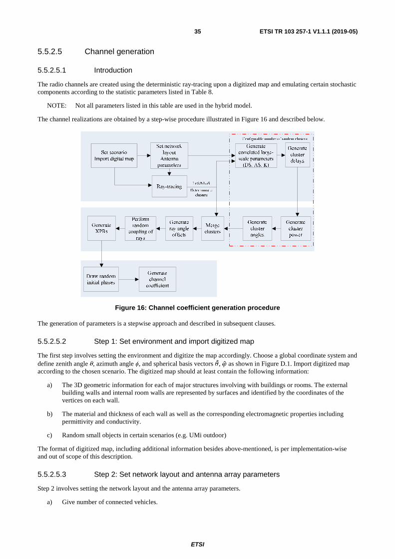
ETSI

ETSI TR 103 257-1 V1.1.1 (2019-05)35

5.5.2.5 Channel generation

5.5.2.5.1 Introduction

The radio channels are created using the deterministic ray-tracing upon a digitized map and emulating certain stochastic components according to the statistic parameters listed in Table 8.

NOTE: Not all parameters listed in this table are used in the hybrid model.

The channel realizations are obtained by a step-wise procedure illustrated in Figure 16 and described below.

Figure 16: Channel coefficient generation procedure

The generation of parameters is a stepwise approach and described in subsequent clauses.

5.5.2.5.2 Step 1: Set environment and import digitized map

The first step involves setting the environment and digitize the map accordingly. Choose a global coordinate system and define zenith angle θ, azimuth angle ϕ, and spherical basis vectors �, �� as shown in Figure D.1. Import digitized map according to the chosen scenario. The digitized map should at least contain the following information:

a) The 3D geometric information for each of major structures involving with buildings or rooms. The external building walls and internal room walls are represented by surfaces and identified by the coordinates of the vertices on each wall.

b) The material and thickness of each wall as well as the corresponding electromagnetic properties including permittivity and conductivity.

c) Random small objects in certain scenarios (e.g. UMi outdoor)

The format of digitized map, including additional information besides above-mentioned, is per implementation-wise and out of scope of this description.

5.5.2.5.3 Step 2: Set network layout and antenna array parameters

Step 2 involves setting the network layout and the antenna array parameters.

a) Give number of connected vehicles.

ETSI

ETSI TR 103 257-1 V1.1.1 (2019-05)36

b) Give 3D locations of connected vehicles, and calculate LOS AOD (ϕLOS,AOD), LOS ZOD (θLOS,ZOD), LOS AOA (ϕLOS,AOA), LOS ZOA (θLOS,ZOA) of each TX and RX pair in the global coordinate system

c) Give TX and RX antenna field patterns Frx and Ftx in the global coordinate system and array geometries

d) Give TX and RX array orientations with respect to the global coordinate system. TX array orientation is defined by three angles ΩTX,α (TX bearing angle), ΩTX,β (TX downtilt angle) and ΩTX,γ (TX slant angle). RX array orientation is defined by three angles ΩRX,α (RX bearing angle), ΩRX,β (RX downtilt angle) and ΩRX,γ (RX slant angle). Give rotational motion of RX in terms of its bearing angle, downtilt angle and slant angle if RX rotation is modelled.

e) Give speed and direction of motion of RX in the global coordinate system for virtual motion.

f) Give system centre frequency/frequencies and bandwidth(s) for each of the connected vehicle links

If the bandwidth (denoted as �) is greater than c/D Hz, where c is the speed of light and D is the maximum antenna aperture in either azimuth or elevation, the whole bandwidth is split into �� equal-sized frequency bins, where

�� ≥ � �� �⁄ is a per-implementation parameter taking into account the channel constancy as well as other potential

evaluation needs, and the bandwidth of each frequency bin is !� =���

. Within k-th frequency bin, the channel power

attenuation, phase rotation, Doppler are assumed constant, whose corresponding values are calculated based on the

centre frequency of k-th frequency bin" = "� −���� !�

� !� for 1 ≤ # ≤ ��, where "� is the centre frequency of the

corresponding TX-RX link.

5.5.2.5.4 Step 3: Apply ray-tracing to each pair

In this step ray-tracing is applied to each pair of link ends (i.e. end-to-end propagation between pair of TX/RX arrays).

a) Perform geometric calculations in ray-tracing to identify propagation interaction types, including LOS, reflections, diffractions, penetrations and scattering (in case the digitized map contains random small objects), for each propagation path. In general, some maximum orders of different interaction types can be set.

The theoretical principles and procedures of geometric tracing calculations can be found in [i.24], [i.13] and references therein. This description does not intend to mandate new concepts and/or procedures to the conventional ray-tracing algorithms; on the other hand, the implementation-based variations aiming to reduce computation complexity are allowed within limits of acceptable calibration tolerances.

The same geometric calculation is shared among all �� frequency bins.

b) Perform electric field calculations over propagation path, based on identified propagation interaction types (LOS, reflection, diffraction, penetration and scattering) and centre frequencies of frequency bins.

The details of electric field calculation can be found in [i.24], [i.13] and references therein.

The modelling algorithms in geometry and electric field calculations for different propagation interactions are summarized in Table 18.

Table 18: Principles applied in ray-tracing

Geometry calculation Electric field calculation LOS Free space LOS Friis equation [i.24]

Reflection Snell's law with image-based method [i.25] Fresnel equation [i.25] Diffraction Fermat's principle [i.26] UTD [i.27] Penetration Snell's law for transmission through slab [i.28] Fresnel equation [i.25]

Scattering (upon small objects)

Isotropic scattering [i.24] RCS-based scattering coefficient [i.29]

NOTE: For reasons of simplicity and simulation speed, the maximum order of reflection on a path without diffraction is configurable from {1,2,3}; the maximum order of diffraction on a path without reflection is configurable from {1,2}; the path containing both reflection and diffraction has 1-order reflection and 1-order diffraction, besides any potential penetrations; and the maximum order of penetration on a path is configurable, with the recommended value equal to 5.

ETSI

ETSI TR 103 257-1 V1.1.1 (2019-05)37

The outputs from Step 3 should at least contain the following for each pair of link ends:

a) the LOS/NLOS flag to indicate whether a LOS propagation mechanism exists;

b) the number of deterministic propagation paths $"� (also referred as deterministic clusters in Step 8. To avoid the unnecessary computation complexity, these $"�deterministic paths only include those paths whose powers are higher than 25 dB below the maximum deterministic path power, where the path power is denoted as %#��"�,�$%# and defined below);

c) for each deterministic path (&"�-th path sorted in ascending order of path delay):

i) the flag indicating whether the deterministic path is generated with scattering upon random small objects;

ii) the normalized path delay ( )RT

RTRTRT l

ll

RTl τττ ′−′= min and the first arrival absolute delay'()�*�′� (with * ′

#��

to be the real absolute propagation delay of the path);

iii) angles of arrival and departure [i.17];

iv) the power %#��, "�,�$%# for k-th frequency bin, and the path power %#��"�,�$%# =

���

∑ %#��, "�,�$%#��

&�

v) the XPR �#��"� of the path, where �#��"� =���

∑ �#��, "���

&� with �#��, "� being the XPR for k-th frequency bin.

vi) to support for true motion, i.e. the case when a trajectory is specified for both TX and RX, a path ID is associated for each deterministic path. The same ID is associated for a path across a number of TX and RX locations as far as 1) it has same interaction types in the same order and 2) its interactions occur in same walls or other surfaces.

The $"� deterministic paths are sorted by normalized path delay (*#��"� ) in ascending order. That is to say, *�"�= 0.

If $"�=0 for a pair of link ends, the channel gain for this pair of link ends is assumed to be zero and the remaining steps are skipped with none of random cluster.

5.5.2.5.5 Step 4: Generate large scale parameters

Generate large scale parameters such as delay spread, angular spreads and Ricean K factor for random clusters.

The generation of large scale parameters takes into account cross correlation according to Table 1 and uses the procedure described in clause 3.3.1 of [i.17] with the square root matrix�,'�'(0)being generated using the Cholesky decomposition and the following order of the large scale parameter vector: sM = [sK, sDS, sASD, sASA, sZSD, sZSA]T. Limit random RMS azimuth arrival and azimuth departure spread values to 104 degrees, i.e. ASA= min(ASA ,104°), ASD = min(ASD ,104°). Limit random RMS zenith arrival and zenith departure spread values to 52 degrees, i.e. ZSA = min(ZSA,52°), ZSD = min(ZSD,52°). For the parameter selection from Table 1, the LOS/NLOS condition determined in Step 3 is applied.

5.5.2.5.6 Step 5: Generate delays for random clusters

Generate delays (denoted as {*"(}) for random clusters.

Delays are drawn randomly according to the exponential delay distribution

* ′

� = −-)"( &)�.�� (37)

where -)"( = '/0 1-) ,�

���∑ *#��"����#��&� 2, Xn ~ uniform(0,1), and cluster index n = 0,…, $*"( with $*"( to be

configurable. A recommended value for $′

"( is the number of clusters given in Table 1.

-) = 3)DS +���

�′

��!��3)DS −

����

∑ *#��"����#��&� �, where rτ is the delay distribution proportionality factor given in Table 8.

Normalize the delays by subtracting the minimum delay and sort the normalized delays to ascending order:

*� = sort�* ′

� − '()�* ′

��� ,)⁄ (38)

ETSI

ETSI TR 103 257-1 V1.1.1 (2019-05)38

where ,) is the additional scaling of delays to compensate for the effect of LOS peak addition to the delay spread, and is depending on the heuristically determined Ricean K-factor [dB] as generated in Step 4:

,) = 10,7705 − 0,0433� + 0,0002�� + 0,000017�+ LOS condition1 NLOS condition

(39)

For the delay used in cluster power generation in Step 6, the scaling factor �� is always 1.

The n-th random cluster is removed if n=0 or ��� − ������ � < ��ℎ for any of 1≤lRT≤LRT, where τth is given by ��ℎ =

��⋅′���∑ ��� − �����′����� , and 0p is the configurable probability for cluster inter-arrival interval to be less than τth. For

example, set 0p =0,2 to obtain τth=0,223 RCτμ .

Denote ���� for 1≤n≤LRC as the delays of the LRC random clusters that remain after the cluster removal.

5.5.2.5.7 Step 6: Generate powers for random clusters

Generate powers (denoted as realRCiP , for 1≤i≤LRC) for random clusters.

Cluster powers for the random clusters are calculated assuming a single slope exponential power delay profile. First, the virtual powers (denoted as � ��,� ����� for 1≤i≤LRC) of random clusters and virtual powers (denoted as ����,� ����� for 1≤j≤LRT) of deterministic clusters are calculated as following.

Denote:

�� = �� −� �� �����DS� ⋅ 10���,��� (40)

��� = �� −���� �����DS� ⋅ 10��,��

� (41)

where Ζi,RC and Ζj,RT are the per cluster shadowing terms in [dB] and meet distribution of N(0, ζ2 ). Then,

� �� ,� ����� =���� ⋅

����∑ ���������� �∑ ������

��

(42)

����,� ����� =���� ⋅

���∑ ���������� �∑ ������

��

+���� ⋅ ��� − 1� (43)

In the case of LOS condition, A=KR with KR being the Ricean K-factor obtained in Step 4 and converted to linear scale; otherwise, A=0. The real power (including effects of pathloss) per random cluster in k-th frequency bin is given by:

� ,��� ,���� =∑ �,

��,���������∑ ���,����������

��

⋅ � �� ,� ����� (44)

for 1≤i≤LRC and 1 ≤ � ≤ ��. Similar to path power of deterministic cluster, the path power of i-th random cluster is calculated as:

� �� ,���� =���∑ � ,��� ,��������� (45)

5.5.2.5.8 Step 7: Generate arrival angles and departure angles

Generate arrival angles and departure angles for both azimuth and elevation, for each random cluster.

For azimuth angles of the n-th random cluster, the composite PAS in azimuth of all random clusters is modelled as wrapped Gaussian (see Table 1). The AOAs are determined by applying the inverse Gaussian function with input parameters ���� ,����and RMS angle spread ASA:

�′�,��� =

�(ASA/�.�)� �������,���� �!�,"����,����

,���,����#$ %�� (46)

ETSI

ETSI TR 103 257-1 V1.1.1 (2019-05)39

with constant �& defined as:

�& = ��&NLOS ⋅ �1,1035 − 0,028� − 0,002�� + 0,0001�'� for LOS�&NLOS for NLOS (47)

where �&NLOS is defined as a scaling factor related to the total number of clusters and is given in Table 9.

In the LOS case, constant �& also depends on the Ricean K-factor K in [dB], as generated in Step 4. Additional scaling of the angles is required to compensate for the effect of LOS peak addition to the angle spread.

Assign positive or negative sign to the angles by multiplying with a random variable Xn with uniform distribution to the discrete set of {1,-1}, and add component �� ~� �0, �ASA 7⁄ ��� to introduce random variation:

��,��� = ���′�,��� + �� + �(�����,��� (48)

where �(�����,���is calculated as:

�(�����,��� = arg�∑ ����,���� ⋅ ������,����� ������ � (49)

Note that ��,����� are given in radians here.

The generation of AOD (φn,AOD) follows a procedure similar to AOA as described above.

For zenith angles of the n-th random cluster, the generation of ZOA assumes that the composite PAS in the zenith dimension of all random clusters is Laplacian (see Table 8). The ZOAs are determined by applying the inverse Laplacian function with input parameters ���� ,���� and RMS angle spread ZSA

� ′�,)�� = −ZSA �������,���� �!

�,"����,����

,���,����#$ %�� (50)

with �* defined as:

�* = ��*NLOS ⋅ �1,3086 + 0,0339� − 0,0077�� + 0,0002�'� for LOS�*NLOS for NLOS (51)

where �*NLOS is a scaling factor related to the total number of clusters and is given in Table 11.

In the LOS case, constant �* also depends on the Ricean K-factor K in [dB], as generated in Step 4. Additional scaling of the angles is required to compensate for the effect of LOS peak addition to the angle spread.

Assign positive or negative sign to the angles by multiplying with a random variable Xn with uniform distribution to the discrete set of {1,-1}, and add component �� ~� �0, �ZSA 7⁄ ��� to introduce random variation

��,)�� = ��� ′�,)�� + �� + �)�� (52)

where �)�� = �(�����,)�� and �(�����,)�� is calculated as:

�(�����,)�� = ����∑ ����,���� ⋅ ������,)���� ������ � (53)

Note that ��,)���� are given in radians here.

The generation of ZOD follows the same procedure as ZOA described above for all states (LOS, NLOS, NLOSv).

5.5.2.5.9 Step 8: Merge deterministic clusters and random clusters

This step involves merging deterministic clusters and random clusters.

First, remove any deterministic or random cluster with less than -25 dB power compared to max{����,���� , realRCiP , } for

all 1≤j≤LRT and 1≤i≤LRC. Then, simply put the remaining deterministic clusters and random clusters into single set of clusters, and meanwhile maintain an attribute for each cluster to indicate whether the cluster is a deterministic cluster or a random cluster.

ETSI

ETSI TR 103 257-1 V1.1.1 (2019-05)40

5.5.2.5.10 Step 9: Generate ray delays and ray angle offsets

Generate ray delays and ray angle offsets inside each cluster, where the cluster can be either random or deterministic.

Denote M as the number of rays per cluster, where M=1 if the cluster corresponds to n=1 in the LOS case, otherwise the value of M is given in Table 1.

When �� = 1:

The relative delay of m-th ray within n-th cluster is given by � ′�, = 0 for m = 1,…, M.

The azimuth angle of arrival (AOA) for the m-th ray in n-th cluster is given by:

��, ,��� = ��,��� + ��+� (54)

where ��+� is the cluster-wise rms azimuth spread of arrival angles (cluster ASA) in Table 1, and offset angle αm is given in Table 10. ��,��� equals to the AOA angle output from Step 3 if n-th cluster is deterministic cluster, and equals to the AOA angle (48) in Step 7 if n-th cluster is random cluster.

The generation of AOD (φn,m,AOD) follows a procedure similar to AOA as described above.

The ZOA for the m-th ray in n-th cluster is given by:

��, ,)�� = ��,)�� + �)+� (55)

where �)+� is the cluster-wise rms spread of ZOA (cluster ZOA) in Table 1 and offset angle αm is given in Table 10. Assuming that ��, ,)�� is wrapped within [0, 360°], if ��, ,)�� ∈ [180°, 360°], then��, ,)��is set to (360° − ��, ,)��). ��,)�� equals to the ZOA angle output from Step 3 if n-th cluster is deterministic cluster, and equals to the ZOA angle (52) in Step 7 if n-th cluster is random cluster.

The generation of ZOD follows the same procedure as ZOA described above.

When �� > 1:

The relative delay of m-th ray within n-th cluster is given by �,�, = sort �-�, − !"#�. ./$�-�, %� that are sorted in

ascending order, where �-�, ~& nif�0,2�DS�, with the cluster delay spread as given in Table 1. unif��, '� denotes the continuous uniform distribution on the interval (�, '). Note that �″�, will be independently generated.

The azimuth angles (AOA and AOD) and zenith angles (ZOA and ZOD) for the m-th ray in n-th cluster in each frequency bin is given by:

ZODmnZODnZODmn

ZOAmnZOAnZOAmn

AODmnAODnAODmn

AOAmnAOAnAOAmn

,,,,,

,,,,,

,,,,,

,,,,,

θθθθθθφφφφφφ

′+=

′+=

′+=

′+=

(56)

for m = 1,…,M, where ��,{���|��0}and ��,{)��|)�0} equal to the {AOA,AOD} and {ZOA, ZOD} angle outputs from Step 3 if n-th cluster is deterministic cluster, and equal to the {AOA,AOD} and {ZOA, ZOD} angle in Step 7 if n-th cluster is random cluster; and

�,�, ,��� ~ 2 �ASAunif�−1,1� �,�, ,��0 ~ 2 �ASDunif�−1,1� �,�, ,)�� ~ 2 �ZSAunif�−1,1�

�,�, ,)�0 ~ 2 �ZSDunif�−1,1� (57)

with the respective cluster angular spreads as given in Table 1.

Assuming that ��, ,)��is wrapped within [0, 360°], if ��, ,)�� ∈ [180°, 360°], then��, ,)��is set to (360° − ��, ,)��).

ETSI

ETSI TR 103 257-1 V1.1.1 (2019-05)41

5.5.2.5.11 Step 10: Generate power of rays in each cluster

Generate power of rays in each cluster, where coupling of rays within a cluster for both azimuth and elevation could be needed.

Given ��,� as the real power in k-th frequency bin for the n-th cluster (either deterministic or random) obtained from Step 8 (see clause 5.5.2.5.9).

When �� = 1, couple randomly AOD angles φn,m,AOD to AOA angles φn,m,AOA within a cluster n. Couple randomly ZOD angles ��, ,)�0 with ZOA angles ��, ,)��using the same procedure. Couple randomly AOD angles φn,m,AOD with ZOD angles ��, ,)�0within a cluster n.

The power of m-th ray in n-th cluster and in k-th frequency bin is given by ��, ,� = ��,� *⁄ for m = 1,…,M.

When �� > 1, the power of m-th ray in n-th cluster and in k-th frequency bin is given by ��, ,� = ��,� ⋅�′

�,�∑ �′�,�����

for

m = 1,…,M, where:

′−

′−⋅

′−

′−

′−=′

ZSD

,,

ZSA

,,

ASD

,,

ASA

,,

DS

,,

2exp

2exp

2exp

2expexp

cc

cccP

ZODmnZOAmn

AODmnAOAmnmnmn

θθ

φφτ

(58)

and �DS, �ASA, �ASD, and �ZSA are respectively the intra-cluster delay spread and the corresponding intra-cluster angular spreads that are given in Table 1. The cluster zenith spread of departure corresponds to �ZSA.

5.5.2.5.12 Step 11: Generate XPRs

Generate the cross polarization power ratios (XPR) κ for each ray m of each cluster n. XPR is log-Normal distributed. Draw XPR values as:

+�, = 101�,�/�2 (59)

where ��, ~� (,XPR,-XPR� ) is Gaussian distributed with -XPR given from Table 1. If n-th cluster is a deterministic cluster, , = 10 ./��2 +����� ; otherwise, , = ,XPR is given in Table 1.

NOTE: ��, is independently drawn for each ray and each cluster.

5.5.2.5.13 Step 12: Draw initial random phases

Draw random initial phase $0�, ** ,0�, *& ,0�, &* ,0�, && % for each ray m of each cluster n and for four different polarization combinations (θθ, θϕ, ϕθ, ϕϕ). The distribution for initial phases is uniform within (-π,π).

In the LOS case, calculate an initial phase 032 λπ DLOS d−=Φ for both θθ and ϕϕ polarizations, where d3D is the 3D

distance between transmitter and receiver and λ0=c/fc is the wavelength of the modelled propagation link.

5.5.2.5.14 Step 13: Generate channel coefficients

Generate channel coefficients for each cluster n and each receiver and transmitter element pair u, s.

In case of NLOS, the channel coefficients of ray m in cluster n for a link between Rx antenna u and Tx antenna s at time t in k-th frequency bin can be calculated as: 1�,3,�, ,�4�+ �2�

= 34�!,�,*���, ,)�� ,5�, ,����4�!,�,5���, ,)��,5�, ,����6�

7889 exp���, ** � �+�, � exp���, *5 ��+�, � exp���, 5* � exp���, 55 � :;

;< 34�!,3,*���, ,)�0 ,5�, ,��0�4�!,3,5���, ,)�0 ,5�, ,��0�6

ETSI

ETSI TR 103 257-1 V1.1.1 (2019-05)42

=>��, ,� 10�����,�(� )����,�(� ,�)�

? exp @�2A 6 ( ��̂�!,�, �C�̅!,� + �̂�!,�, �C�̅!,3�E exp��2AF�, ,�2� (60)

where Frx,u,θ and Frx,u,ϕ are the receive antenna element u field patterns in the direction of the spherical basis vectors, �G and �H respectively, Ftx,s,θ and Ftx,s,ϕ are the transmit antenna element s field patterns in the direction of the spherical basis vectors, �G and �H respectively. Note that the patterns are given in the GCS and therefore include transformations with respect to antenna orientation as described in Annex C. The delay (TOA) for ray m in cluster n for a link between Rx antenna u and Tx antenna s is given by:

��,3,�, = �� + � ′�, −�( �̂�!,�, � .CI�!,� −

�( �̂�!,�, � .CI�!,3 (61)

For the m-th ray within n-th cluster, �̂�!,�, is the spherical unit vector with azimuth arrival angle ��, ,��� and elevation arrival angle ��, ,)��, given by:

�̂�!,�, = JK"#��, ,)�� �/K��, ,���K"#��, ,)�� K"#��, ,����/K��, ,)��L (62)

�̂�!,�, is the spherical unit vector with azimuth departure angle ��, ,��0 and elevation departure angle ��, ,)�0, given by:

�̂�!,�, = JK"#��, ,)�0 �/K��, ,��0K"#��, ,)�0 K"#��, ,��0�/K��, ,)�0L (63)

Also, CI�!,�is the location vector of receive antenna element u and CI�!,3is the location vector of transmit antenna element s, κn,m is the cross polarization power ratio in linear scale. If polarization is not considered, the 2x2 polarization matrix can be replaced by the scalar ����0�, � and only vertically polarized field patterns are applied.

The Doppler frequency component is calculated from the angles of TX and scatterer and RX and scatterer. Furthermore, the velocity vector of the TX and the velocity vector of the RX.

For sidelink, dual mobility is modeled as follows with the parameters defined in [i.13]:

a) Doppler for the LOS path:

F�+,� = 6 ( ��̂�!,�+�M̅�! + �̂�!,�+�M̅�!�

b) Deterministic calculation of Doppler for the delayed paths:

M�, ,� =6 ( ��̂�!,�, � ∙ M̅�! + �̂�!,�, � ∙ M̅�! + 2 �, N�, �

where N�, is a random variable with uniform distribution from −M3(��� to M3(���, M3(��� is the maximum speed of the vehicle in the layout, and �, (0 ≤ �, ≤ 1) is a random variable with uniform distribution. Evaluation using other distribution for �, is not precluded.

c) Stochastic calculation of Doppler for the delayed paths [i.23]:

i) Definition of scatter belts Δi, i=1,…, 4 indicated in blue in Figure 17. This is the geometric area, where the scatterers are randomly distributed.

ii) Select discrete delay range (ellipse in Figure 18 represents one specific delay).

iii) Compute delay-dependent Doppler pdf for each selected delay.

iv) Randomly draw M�, ,� from the pdf computed in the previous step.

[ ]Trxvrxvrxvrxvrxvrxrx vv ,,,,, cossinsincossin θφθφθ=

[ ]Ttxvtxvtxvtxvtxvtxtx vv ,,,,, cossinsincossin θφθφθ=

ETSI

ETSI TR 103 257-1 V1.1.1 (2019-05)43

Figure 17: Definition of coordinate system and scatter belts

As an example for the rural V2V communication channel, measurement based parameters of the scatter belts are provided in Table 19.

Table 19: Scatter belt values for a rural scenario extracted from measurement data [i.24]

Scatter Belt Value [m] Δ1 3,75 Δ2 11,25 Δ3 3,75 Δ4 11,25

For up- and downlink connections to RSUs, the above equations for Doppler frequency components simplify due to fixed location of the RSUs as M�! = 0 or M�! = 0, respectively.

In case of LOS, the channel coefficient is calculated in the same way as in Equation (60) except for n = 1:

1�,3,���,��+ �2� = 34�!,�,*���+,)�� ,5�+,����4�!,�,5���+,)�� ,5�+,����6� Oexp���+� 0

0 − exp��Φ�+�P 34�!,3,*���+,)�0 ,5�+,��0�4�!,3,5���+,)�0 ,5�+,��0�6 =>��,� 10

�����,���(� )����,���(� ,�)� ? exp @�2A 6 ( ��̂�!,�, �C�̅!,� + �̂�!,�, �C�̅!,3�E exp��2AF�+,�2� (64)

where the corresponding delay (TOA) for cluster n=1 for a link between RX antenna, u, and TX antenna, s, is given by ��,3,��� = �� −�( �̂�!,�+� .CI�!,� −

�( �̂�!,�+� .CI�!,3. The Equation (60) and Equation (64) oxygen absorption loss, OLn,m(f), for each ray, m, in cluster, n, at carrier frequency, f, is modelled as

OLn,m(f) = α(f)/1000 · c · O�� + � ′�, + !"#��� �� ′����P [dB] (65)

where α(f) is the frequency dependent oxygen loss per distance (dB/km), c is speed of light (m/s), and nτ is the delay

(s) obtained from Step 3 for deterministic clusters and from Step 5 (see clause 5.5.2.5.6) for random clusters. !"#���′� is from the output of Step 3 (see clause 5.5.2.5.4).

In Equation (60) and Equation (64) blockage modelling is an add-on feature. If the blockage model is applied, the blockage loss, BLn,m(f,t) in unit of dB, for each ray m in cluster n at carrier frequency f and time t is modelled in the same way as given in clause 5.4.2.4.1; otherwise BLn,m(f,t) = 0 dB for all f and t.

ETSI

ETSI TR 103 257-1 V1.1.1 (2019-05)44

Annex A: Mahler model for tracking multipath components The Mahler model described in [i.7] was first published in 2016. It is a NGSM model based on an intensive measurement campaign made around Berlin, Germany. The channel sounder used for the measurements at a centre frequency at 5,7 GHz had a measurement bandwidth of 1 GHz. This allowed detecting and tracking MPCs with a local resolution of 30 cm. Measurements were done for seven of the proposed scenarios plus measurements for tunnel convoy traffic as presented in Table A.1.

Table A.1: Scenario Matrix for the Mahler channel model

Mahler Urban Rural Highway Oncoming X X X

Convoy X X X RSU X

Further Scenarios: Tunnel convoy Traffic

The number of MPCs and the MPC birth rate (number of new-born MPCs per meter travelled) are both modelled with a distance-dependent Poisson distribution, as shown in Equation A.1.

���|�2, ��, ��,C� =78�8�∙9�8!∙9 :"!! ∙ �� �−��2 + �� ∙ C + �3 ∙ C��� (A.1)

where the set of parameters p0, p1 and p2 is individually defined for all scenarios.

The MPC lifetime is modelled with a Birnbaum-Saunders distribution as shown in Equation A.2.

���|Q, R� =�√�< ∙ S=! >? => !?�@! T ∙ �� U−

A=! >? => !? B �@ V (A.2)

where x > 0 and the set of parameters Q and R is defined individually for all scenarios.

The relative Doppler frequency of new-born MPCs is modelled with a Weibull distribution, as shown in Equation A.3.

M��|W, +� =CD !D�C� ∙ �� − !D�C� (A.3)

where x>0, the parameter W determines the scale and the parameter κ the shape of the curve.

These comprehensive statistics defined in the Mahler channel model allow creating MPCs valid for a certain amount of time. As a result, the Mahler channel model represents correlated scatterer as it can be considered for V2X channels.

ETSI

ETSI TR 103 257-1 V1.1.1 (2019-05)45

Annex B: LOS probability and transition probability curves In relation to define LOS/NLOS conditions in the different scenarios, there exists a need to model the transitions between different states as described in [i.11]. Realistic LOS blockage realization is required to assign the appropriate path loss, shadowing, small-scale, and large-scale parameters over time and space. LOS blockage modelling is particularly important for V2X communication, because of:

• high mobility, possibly on both sides of the link (e.g. in the case of V2V communication), resulting in more dynamic LOS blockage;

• have low antenna heights, resulting in more frequent LOS blockage;

• V2X communication will be used for applications related to safety, either directly (e.g. emergency braking, intersection collision avoidance application [i.12], etc.) or indirectly (e.g. platooning, lane-change manoeuvres, etc.).

The work described in [i.11] designs a time and space consistent model for LOS blockage of V2V channels. It models the evolution of states using Markov chain. The three-state discrete-time Markov chain was used, comprised of the following states:

i) Line-of-Sight (LOS);

ii) non-LOS due to static objects, e.g. buildings, trees, etc. (NLOSb); and

iii) non-LOS due to mobile objects (vehicles) (NLOSv).

Results presented in [i.11] showed significant difference compared to standard cellular models for LOS blockage, thus emphasizing the need for bespoke modelling of blockage for V2X links, see Figure B.1.

Figure B.1: Markov chain for modelling the time evolution of V2V links

According to [i.11] the propagation condition of V2V links can be modelled using three states:

i) LOS;

ii) NLOSb - non-LOS due to static objects (e.g. buildings, trees, etc.); and

iii) NLOSv - non-LOS due to mobile objects (vehicles).

A Markov chain comprised of three states (LOS, NLOSb, NLOSv) is proposed for system level simulations to ensure time consistent modelling of V2V channels.

To provide a tractable model for generation of time-evolved V2V links, in [i.11] curve fitting was performed for LOS and transition probabilities. The main curves are shown in Annex B. This resulted in two sets of equations, one from LOS probabilities curves (Table II in [i.11]) and the second set for transition probabilities (Table III in in [i.11]), see Table B.1.

ETSI

ETSI TR 103 257-1 V1.1.1 (2019-05)46

Table B.1: LOS probability equations for highway and urban environment, medium density

NOTE: For transition probabilities, the equations listed in Table III in [i.11] can be applied.

Figure B.2, Figure B.3, Figure B.4 and Figure B.5 show the LOS probability and transition probability curves for Markov model as derived in [i.11].

Figure B.2: LOS probabilities in urban environment, medium density

Figure B.3: LOS probabilities on highway, medium density

ETSI

ETSI TR 103 257-1 V1.1.1 (2019-05)47

Figure B.4: Transition probabilities in urban environment, medium density

Figure B.5: Transition probabilities on A6 highway, medium density

ETSI

ETSI TR 103 257-1 V1.1.1 (2019-05)48

Annex C: Coordinate system

C.1 Definition A coordinate system is defined by the x, y, z axes, the spherical angles and the spherical unit vectors as shown in Figure C.1. Figure C.1 defines the zenith angle � and the azimuth angle� in a Cartesian coordinate system. Note that � = 0points to the zenith and � = 90�points to the horizon. The field component in the direction of �� is given by ��and the field component in the direction of �� is given by ��.

n̂

θ̂

φ̂θ

z

x

yφ

Figure C.1: Definition of spherical angles and spherical unit vectors in a Cartesian coordinate system, where��is the given direction, � and � are the spherical basis vectors

C.2 Local and global coordinate systems A Global Coordinate System (GCS) is defined for a system comprising multiple vehicles, RSUs, pedestrians and BSs. An array antenna for a BS or a UT can be defined in a Local Coordinate System (LCS). An LCS is used as a reference to define the vector far-field that is pattern and polarization, of each antenna element in an array. It is assumed that the far-field is known in the LCS by formulae. The placement of an array within the GCS is defined by the translation between the GCS and a LCS. The orientation of the array with respect to the GCS is defined in general by a sequence of rotations (described in subsequent clause). Since this orientation is in general different from the GCS orientation, it is necessary to map the vector fields of the array elements from the LCS to the GCS. This mapping depends only on the orientation of the array and is given by the equations in subsequent clause. Note that any arbitrary mechanical orientation of the array can be achieved by rotating the LCS with respect to the GCS.

C.3 Transformation from a LCS to a GCS A GCS with coordinates (x, y, z, �, �) and unit vectors (��, ��) and an LCS with "primed" coordinates (x', y', z', �′, �′) and "primed" unit vectors (��′, �� ′) are defined with a common origin in Figures C.2 and C.3. Figure C.3 illustrates the sequence of rotations that relate the GCS (gray) and the LCS (blue). Figure C.4 shows the coordinate direction and unit vectors of the GCS (gray) and the LCS (blue). Note that the vector fields of the array antenna elements are defined in the LCS. In Figure C.3 an arbitrary 3D-rotation of the LCS with respect to the GCS given by the angles α, β, γ is considered. The set of angles α, β, γ can also be termed as the orientation of the array antenna with respect to the GCS.

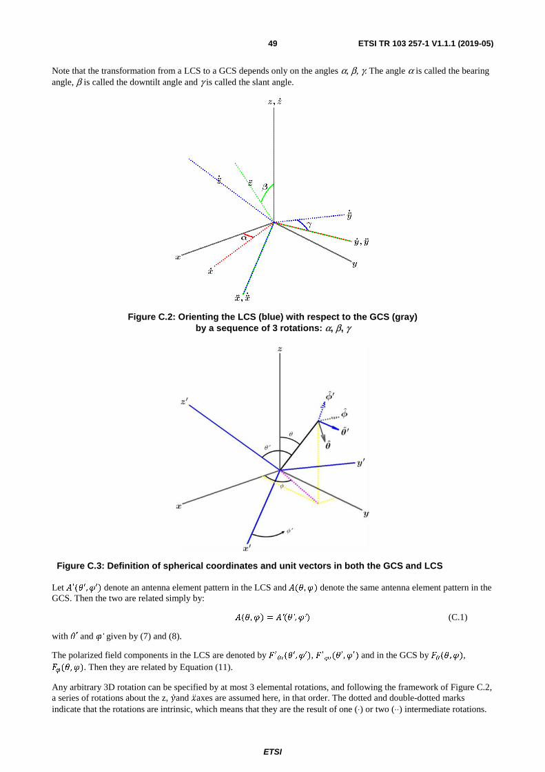
ETSI

ETSI TR 103 257-1 V1.1.1 (2019-05)49

Note that the transformation from a LCS to a GCS depends only on the angles α, β, γ. The angle α is called the bearing angle, β is called the downtilt angle and γ is called the slant angle.

Figure C.2: Orienting the LCS (blue) with respect to the GCS (gray) by a sequence of 3 rotations: α, β, γ

Figure C.3: Definition of spherical coordinates and unit vectors in both the GCS and LCS

Let �′��′, �′� denote an antenna element pattern in the LCS and ���, �� denote the same antenna element pattern in the GCS. Then the two are related simply by:

���, �� � �′��′, �′� (C.1)

with �′ and �′ given by (7) and (8).

The polarized field components in the LCS are denoted by �����′, �′�,

�����′, �′� and in the GCS by ���, ��,

���, ��. Then they are related by Equation (11).

Any arbitrary 3D rotation can be specified by at most 3 elemental rotations, and following the framework of Figure C.2, a series of rotations about the z, �and � axes are assumed here, in that order. The dotted and double-dotted marks indicate that the rotations are intrinsic, which means that they are the result of one (⋅) or two (⋅⋅) intermediate rotations.

ETSI

ETSI TR 103 257-1 V1.1.1 (2019-05)50

In other words, the �� axis is the original y axis after the first rotation about z, and the � axis is the original x axis after the first rotation about z and the second rotation about�� . A first rotation of α about z sets the antenna bearing angle (i.e. the sector pointing direction for a BS antenna element). The second rotation of β about �� sets the antenna downtilt angle. Finally, the third rotation of γ about � sets the antenna slant angle. The orientation of the x, y and z axes after all three rotations can be denoted as �, �� and ��. These triple-dotted axes represents the final orientation of the LCS, and for notational purposes denoted as the x', y' and z' axes (local or "primed" coordinate system).

In order to establish the equations for transformation of the coordinate system and the polarized antenna field patterns between the GCS and the LCS, it is necessary to determine the composite rotation matrix that describes the transformation of point (x, y, z) in the GCS into point (x', y', z') in the LCS. This rotation matrix is computed as the product of three elemental rotation matrices. The matrix to describe rotations about the z,��and � axes by the angles α, β and γ respectively and in that order is defined as:

� = ��������������� = �+ ��� � − ��� � 0+ ��� � + ��� � 0

0 0 1��+ ��� � 0 + ��� �

0 1 0− ��� � 0 + ��� ���

1 0 00 + ��� � − ��� �0 + ��� � + ��� ��(C.2)

The reverse transformation is given by the inverse of R, which is also equal to the transpose of R since it is orthogonal.

��� = ���−�����−�����−�� = � (C.3)

The simplified forward and reverse composite rotation matrices are given by:

� = ���� � ��� � ��� � ��� � ��� � − ��� � ��� � ��� � ��� � ��� � + ��� � ��� ���� � ��� � ��� � ��� � ��� � + ��� � ��� � ��� � ��� � ��� � − ��� � ��� �− ��� � ��� � ��� � ��� � ��� � � (C.4)

and

��� = � ��� � ��� � ��� � ��� � − ��� ���� � ��� � ��� � − ��� � ��� � ��� � ��� � ��� � + ��� � ��� � ��� � ��� ���� � ��� � ��� � + ��� � ��� � ��� � ��� � ��� � − ��� � ��� � ��� � ��� �� (C.5)

These transformations can be used to derive the angular and polarization relationships between the two coordinate systems.

To establish the angular relationships, consider a point (x, y, z) on the unit sphere defined by the spherical coordinates (ρ=1, θ, φ), where ρ is the unit radius, θ is the zenith angle measured from the +z-axis, and φ is the azimuth angle measured from the +x-axis in the x-y plane. The Cartesian representation of that point is given by:

�� = � �� = ���� � ��� ���� � ��� ���� � � (C.6)

The zenith angle is computed as !"������� ⋅ �̂� and the azimuth angle as !"$( � ⋅ �� + %�� ⋅ ��), where �, �� and �̂ are the Cartesian unit vectors. If this point represents a location in the GCS defined by θ and φ, the corresponding position in the LCS is given by �����, from which local angles θ' and φ' can be computed. The results are given in Equations (C.7) and (C.8).

�′��,�, � ;� ,�� = !"���� &'001( �����) = acos���� � ��� � ��� � + ���� � ��� � ����� − �� −

��� � ����� − ��� ��� �� (C.7)

�′��,�, � ;� ,�� = !"$ &'1%0

( �����) =

arg * ���� � ��� � ����� − �� − ��� � ��� �� +%���� � ��� � ��� � + ���� � ��� � ����� − �� + ��� � ����� − ��� ��� ��+ (C.8)

These formulae relate the spherical angles (θ, φ) of the GCS to the spherical angles (θ', φ') of the LCS given the rotation operation defined by the angles (α, β, γ).

ETSI

ETSI TR 103 257-1 V1.1.1 (2019-05)51

The polarized field components are denoted by ��(�,�), ��(�,�) in the GCS and ��(�′,�′), �′

�′(�′,�′) in the LCS.

These are related by:

*����,������,��+ = �����,����� ′�� ′,�′� ����,����� ′�� ′,�′�����,����� ′�� ′,�′� ����,����� ′�� ′,�′� ��′

�′�� ′,�′��′

�′�� ′,�′� (C.9)

In this equation, �� and �� represent the spherical unit vectors of the GCS, and �� and �� ′are the representations in the LCS. The forward rotation matrix R transforms the LCS unit vectors into the GCS frame of reference. These pairs of unit vectors are orthogonal and can be represented as shown in Figure C.4.

Figure C.4: Rotation of the spherical basis vectors by an angle ψ due to the orientation of the LCS with respect to the GCS

Assuming an angular displacement of ψ between the two pairs of unit vectors, the rotation matrix of Equation (C.9) can be further simplified as:

�����,����� ′�� ′,�′� ����,����� ′�� ′,�′�����,����� ′�� ′,�′� ����,����� ′�� ′,�′� = * ��� , ����- 2⁄ + ,�����- 2⁄ − ,� ��� , + = *+ ��� , − ��� ,+ ��� , + ��� ,+

(C.10)

and Equation (C.9) can be written as:

*����,������,��+ = *+ ��� , − ��� ,+ ��� , + ��� ,+ ��′

�′�� ′,�′��′

�′�� ′,�′� (C.11)

The angle ψ can be computed in numerous ways from Equation (C.10), with one such way approach being:

, = !"$ /����,����� ′�� ′,�′� + %����,����� ′�� ′,�′�0 (C.12)

The dot products are readily computed using the Cartesian representation of the spherical unit vectors. The general expressions for these unit vectors are given by:

�� = ���� � ��� ���� � ��� �− ��� � � (C.13)

and

�� = �− ��� �+ ��� �

0� (C.14)

ETSI

ETSI TR 103 257-1 V1.1.1 (2019-05)52

The angle ψ can be expressed as a function of mechanical orientation (α, β, γ) and spherical position (θ, φ), and is given by:

, = !"$ �1��� � ��� � ����� − �� + ��� � ���� � ��� � − ��� � ��� � ����� − ���2 +%���� � ����� − �� + ��� � ��� � ����� − ��� (C.15)

It can be shown that��� ,and��� ,can be expressed as:

��� , =�� � �� � �� ��� �� � �� � �� ������ �� � �������� �� �

������ � �� � �� ��� �� � �� � �� ������ �� � �������� �� ��� (C.16)

��� , = �� � �� � �������� �� � �� �����

������ � �� � �� ��� �� � �� � �� ������ �� � �������� �� ��� (C.17)

C.4 Transformation from an LCS to a GCS for downtilt angle only

In this clause equations are provided for the transformation from LCS to GCS assuming that the orientation of the LCS (with respect to the GCS) is such that the bearing angle α=0, the downtilt angle β is non-zero and the slant angle γ=0. In other words the y'-axis of the LCS is parallel to the y-axis of the GCS. Considering a BS antenna element the x-axis of the GCS is aligned with the pointing direction of the sector. Mechanical downtilt is modelled as a rotation of the LCS around the y-axis. For zero mechanical downtilt the LCS coincides with the GCS.

This transformation relates the spherical angles (�,�) in the global coordinate system to spherical angles (�′,�′) in the local (antenna-fixed) coordinate system and is defined as follows:

�′ = !"�������� � ��� � ��� � + ��� � ��� �� (C.18)

�′ = !"$���� � ��� � ��� � − ��� � ��� � + % ��� � ��� �� (C.19)

where � is the mechanical tilt angle around the y-axis as defined in Figure C.5. Note that Equations (C.7) and (C.8) reduce to Equations (C.18) and (C.19), if both α and γ are zero.

The antenna element pattern 3(�,�) in the GCS is related to the antenna element pattern 3′(�′,�′) in the LCS by the relation:

3��,�� = 3′��′,�′� (C.20)

with �′ and �′given by Equations (C.18) and (C.19).

n̂

θ̂

φ̂

ψ

'φ̂

'θ̂y

z

x

n̂

β

β

'φ̂

'θ̂θ̂

φ̂

'x

'θ

'y

'z

'φ

Figure C.5: Definition of angles and unit vectors when the LCS has been rotated an angle 4 around the y-axis of the GCS

ETSI

ETSI TR 103 257-1 V1.1.1 (2019-05)53

For a mechanical tilt angle �, the global coordinate system field components ��(�,�) and ��(�,�), are calculated from the field components ��(�′,�′) and �′

�′(�′,�′) of the radiation pattern in the local (antenna-fixed) coordinate system

as:

��(�,�) = �′

�′(�′,�′) ��� , − �′

�′(�′,�′) ��� , (C.21)

��(�,�) = �′

�′(�′,�′) ��� , + �′

�′(�′,�′) ��� , (C.22)

where �′ and �′ are defined as in Equations (C.18) and (C.19), and , is defined as:

, = !"$���� � ��� � − ��� � ��� � ��� � + % ��� � ��� ��. (C.23)

Note that the Equation (C.15) is reduced to equation (C.23) if both α and γ are zero.

As an example, in the horizontal cut, i.e. for � = 90°, Equations (C.18), (C.19) and (C.23) become

�′ = !"�������� � ��� �� (C.24)

�′ = !"$���� � ��� � + % ��� �� (C.25)

, = !"$���� � + % ��� � ��� �� (C.26)

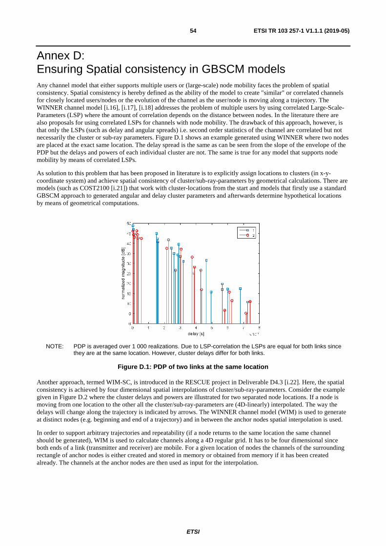
ETSI

ETSI TR 103 257-1 V1.1.1 (2019-05)54

Annex D: Ensuring Spatial consistency in GBSCM models Any channel model that either supports multiple users or (large-scale) node mobility faces the problem of spatial consistency. Spatial consistency is hereby defined as the ability of the model to create "similar" or correlated channels for closely located users/nodes or the evolution of the channel as the user/node is moving along a trajectory. The WINNER channel model [i.16], [i.17], [i.18] addresses the problem of multiple users by using correlated Large-Scale-Parameters (LSP) where the amount of correlation depends on the distance between nodes. In the literature there are also proposals for using correlated LSPs for channels with node mobility. The drawback of this approach, however, is that only the LSPs (such as delay and angular spreads) i.e. second order statistics of the channel are correlated but not necessarily the cluster or sub-ray parameters. Figure D.1 shows an example generated using WINNER where two nodes are placed at the exact same location. The delay spread is the same as can be seen from the slope of the envelope of the PDP but the delays and powers of each individual cluster are not. The same is true for any model that supports node mobility by means of correlated LSPs.

As solution to this problem that has been proposed in literature is to explicitly assign locations to clusters (in x-y-coordinate system) and achieve spatial consistency of cluster/sub-ray-parameters by geometrical calculations. There are models (such as COST2100 [i.21]) that work with cluster-locations from the start and models that firstly use a standard GBSCM approach to generated angular and delay cluster parameters and afterwards determine hypothetical locations by means of geometrical computations.

NOTE: PDP is averaged over 1 000 realizations. Due to LSP-correlation the LSPs are equal for both links since they are at the same location. However, cluster delays differ for both links.

Figure D.1: PDP of two links at the same location

Another approach, termed WIM-SC, is introduced in the RESCUE project in Deliverable D4.3 [i.22]. Here, the spatial consistency is achieved by four dimensional spatial interpolations of cluster/sub-ray-parameters. Consider the example given in Figure D.2 where the cluster delays and powers are illustrated for two separated node locations. If a node is moving from one location to the other all the cluster/sub-ray-parameters are (4D-linearly) interpolated. The way the delays will change along the trajectory is indicated by arrows. The WINNER channel model (WIM) is used to generate at distinct nodes (e.g. beginning and end of a trajectory) and in between the anchor nodes spatial interpolation is used.

In order to support arbitrary trajectories and repeatability (if a node returns to the same location the same channel should be generated), WIM is used to calculate channels along a 4D regular grid. It has to be four dimensional since both ends of a link (transmitter and receiver) are mobile. For a given location of nodes the channels of the surrounding rectangle of anchor nodes is either created and stored in memory or obtained from memory if it has been created already. The channels at the anchor nodes are then used as input for the interpolation.

ETSI

ETSI TR 103 257-1 V1.1.1 (2019-05)55

Figure D.2: PDPs of two links at different locations (with correlated LSPs)

An example of the surrounding rectangle is depicted in Figure D.3. Instead of the full four-dimensional rectangle only a two-dimension subset is shown but the principle is the same for all four dimensions.

Figure D.3: Exemplary network layout of WIM with one mobile-station and associated interpolation grid-points

Figure D.4 shows an example comparing the output of using the WINNER channel model and WIM-SC. The data for the WINNER model was generated by placing multiple users along a 10 meter trajectory since WINNER does not support node mobility. The delay spreads are highly correlated but the cluster delays evolve in a non-spatial-consistent fashion. On the right-hand side of Figure D.4 the output of WIM-SC can be seen. It is apparent that the cluster delays now progress spatial-consistent as the node is moving along the trajectory.

ETSI

ETSI TR 103 257-1 V1.1.1 (2019-05)56

NOTE: Left naive approach using WINNER. Right result using WIM-SC.

Figure D.4: Cluster delays along 10 m trajectory

The overall scheme of how channels are generated in WIM-SC I s depicted in Figure D.5. It can be seen that WIM-SC is built around the WIM implementation and uses its code as much as possible thus reducing the effort of implementing a spatial consistent model. Given that the GBSCM model described in clause 5.4 follows the same implementation principle as WIM, the procedure described in this clause can be used as part of the SLS model clause 5.4.

Figure D.5: Scheme of generating spatial consistent channels

ETSI

ETSI TR 103 257-1 V1.1.1 (2019-05)57

Annex E: Bibliography

• D. Dhoutaut, A. Regis, and F. Spies: "Impact of radio propagation models in vehicular ad hoc networks simulations", in Proceedings of the 3rd International Workshop on Vehicular Ad Hoc Networks (VANET 06), pp. 40-49, Los Angeles, CA, US, September 2006.

• L. Cheng, B. E. Henty, D. D. Stancil, F. Bai and P. Mudalige: "Mobile vehicle-to-vehicle narrow-band channel measurement and characterization of the 5.9 GHz dedicated short range communication (DSRC) frequency band", in IEEE Journal on Selected Areas in Communications, vol. 25, no. 8, pp. 1501-1516, October 2007.

• J. Maurer, T. Fugen, T. Schafer and W. Wiesbeck: "A new inter-vehicle communications (IVC) channel model", in Proceedings of the 60th IEEE Vehicular Technology Conference (VTC2004-Fall), September 2004, pp. 9-13.

• J. Karedal, F. Tufvesson, N. Czink, A. Paier, C. Dumard, T. Zemen, C. Mecklenbrauker, and A. Molisch: "A geometry-based stochastic MIMO model for vehicle-to-vehicle communications", in IEEE Transactions on Wireless Communications, vol. 8, no. 7, pp. 3646-3657, July 2009.

• X. Cheng, C.-X. Wang, D. I. Laurenson, S. Salous, and A. V. Vasilakos: "An adaptive geometry-based stochastic model for non-isotropic MIMO mobile-to-mobile channels", in IEEE Transactions on Wireless Communications, vol. 8, no. 9, pp. 4824-4835, October 2009.

• R. He, O. Renaudin, V.-M. Kolmonen, K. Haneda, Z. Zhong, B. Ai and C. Oestges: "A Dynamic Wideband Directional Channel Model for Vehicle-to-Vehicle Communications", in IEEE Transactions on Industrial Electronics, vol. 62, no. 12, p. 7870-7882, December 2015.

• A. F. Molish: "Wireless Communications", Second Edition, Wiley, 2011.

• H. Boeglen, B. Hilt, P. Lorenz, J. Ledy and A. M. Poussard: "A survey of V2V channel 57odelling for VANET simulations", in Proceedings of 2011 Eighth International Conference on Wireless On-Demand Network Systems and Services (WONS 2011), Bardonecchia, Italy, January 2011, pp. 117-123.

• I. Sen and D. W. Matolak: "Vehicle-vehicle channel models for the 5 GHz band", in IEEE Transactions on Intelligent Transportation Systems, vol. 9, no. 2, pp. 235-245, June 2008.

• L.-C. Wang, W.-C. Liu, and Y.-H. Cheng: "Statistical analysis of a mobile-to-mobile Rician fading channel model", in IEEE Transactions on Vehicular Technology, vol. 58, no. 1, pp. 32-38, January 2009.

• A. Zajic, G. Stuber, T. Pratt, and S. Nguyen: "Wideband MIMO mobile-to-mobile channels: Geometry-based statistical modeling with experimental verification", in IEEE Transactions on Vehicular Technology, vol. 58, no. 2, pp. 517-534, February 2009.

• M. Patzold, B. O. Hogstad, ad N. Youssef: "Modeling, analysis, and simulation of MIMO mobile-to-mobile fading channels", in IEEE Transactions on Wireless Communications, vol. 7, no. 2, February 2008.

• A. G. Zajic and G. L. Stuber: "Space-time correlated mobile-to-mobile channels: Modelling and simulation", in IEEE Transaction on Vehicular Technology, vol. 57, no. 2, pp. 715-726, March 2008.

• A. Paier et al.: "Car-to-car radio channel measurements at 5 GHz: Path loss, power-delay profile, and delay-Doppler spectrum," in the Proceedings of the 4th International Symposium on Wireless Communication Systems, Trondheim, Norway, October 2007, pp. 224-228.

• J. Maurer, T. Fugen, and W. Wiesbeck: "Narrowband measurement and analysis of the inter-vehicle transmission channel at 5.2 GHz", in Proceedings of the 2002 IEEE 55th Vehicular Technology Conference (VTC Spring 2002), Birmingham, AL, US, August 2002, pp. 1274-1278.

• J. Maurer, T. Fugen, T. Schafer, and W. Wiesbeck: "A new inter-vehice communications (IVC) channel model", in Proceedings of the 2004 IEEE 60th Vehicular Technology Conference (VTC2004-Fall), Los Angeles, CA, US, April 2004, pp. 6-9.

ETSI

ETSI TR 103 257-1 V1.1.1 (2019-05)58

• W. Wiesbeck and S. Knorzer: "Characteristics of the mobile channel for high velocities", in Proceedings of the 2007 International Conference on Electromagnetics in Advanced Applications (ICEAA 2007), Torino, Italy, September 2007, pp. 116-120.

• A. Molisch, F. Tufvesson, J. Karedal, and C. Mecklenbrauker: "A survey on vehicle-to-vehicle propagation channels", in IEEE Wireless Communications, vol. 16, no. 6, pp. 12-22, 2009.

• T Abbas, K Sjöberg, J Karedal, F Tufvesson: "Measurement based shadow fading model for vehicle-to-vehicle network simulations", arXiv preprint, arXiv:1203.3370v2, 2012.

• G. Acosta-Marum and M. A. Ingram: "Six time- and frequency- selective empirical channel models for vehicular wireless LANs", in IEEE Vehicular Technology Magazine, vol. 2, nr. 4, p. 4-11, December 2007.

• M. Nilsson, et al.: "A Measurement Based Multilink Shadowing Model for V2V Network Simulations of Highway Scenarios", IEEE Transactions on Vehicular Technology (2017).

• RESCUE project deliverable D4.3: "Report on channel analysis and modeling".

NOTE: Available at: https://cordis.europa.eu/docs/projects/cnect/5/619555/080/deliverables/001-D43v10FINAL.pdf.

• Schneider, Christian et al.: "Directional analysis of multipath propagation in vehicle-2-vehicle channels", in IEEE Xplore digital library, 2016.

• M. Walter, T. Zemen and D. Shutin: "Empirical relationship between local scattering function and joint probability density function", 2015 IEEE 26th Annual International Symposium on Personal, Indoor, and Mobile Radio Communications (PIMRC), Hong Kong, 2015, pp. 542-546.

• M. Walter, D. Shutin and A. Dammann: "Time-Variant Doppler PDFs and Characteristic Functions for the Vehicle-to-Vehicle Channel", in IEEE Transactions on Vehicular Technology, vol. 66, no. 12, pp. 10748-10763, Dec. 2017.

• M. Walter, D. Shutin and U. C. Fiebig: "Delay-Dependent Doppler Probability Density Functions for Vehicle-to-Vehicle Scatter Channels", in IEEE Transactions on Antennas and Propagation, vol. 62, no. 4, pp. 2238-2249, April 2014.

ETSI

ETSI TR 103 257-1 V1.1.1 (2019-05)59

History

Document history

V1.1.1 May 2019 Publication