Ethnicity, Community and Local Public Good …ices.gmu.edu/wp-content/uploads/2010/07/Spring2010...1...
42
0 Ethnicity, Community and Local Public Good Provision Angela C. M. de Oliveira 1 *, Catherine C. Eckel 2 and Rachel T. A. Croson 2 1 University of Massachusetts Amherst, 2 University of Texas at Dallas This Draft: 4/15/10 This is a very early draft, please do not cite without the authors’ permission. Abstract: Ethno-linguistic diversity (or fractionalization) has been found to negatively impact public goods provision, however many underlying causes may exist for the observed impact. We conduct a field experiment in three low-income, minority neighborhoods to investigate the impacts of ethnicity and community-level ethnic heterogeneity on the voluntarily provision of local public goods. Participants make provision decisions to organizations that are active in the improvement efforts of their community (health services, children’s education, and job training). We complement the existing literature by providing a “deep” view of several communities and by including variables not traditionally included in the analysis due to data limitations (including preferences, perceptions, and beliefs). We examine the likelihood of contributing and amount contributed and find that ethnic heterogeneity negatively impacts the individual decision to provide local public goods in our baseline model, but that (contrary to the previous literature) it loses significance once a richer set of variables are taken into account. Further, the key variables leading to the observed differences between Hispanics and African Americans in our sample are differences in beliefs and patience across the two samples. Keywords: Public Goods, Ethnicity, Community Characteristics, Poverty, Cooperation JEL Classifications: C93, H41, D64 *Corresponding author. [email protected] or [email protected], Department of Resource Economics, Isenberg School of Management, University of Massachusetts Amherst, 212G Stockbridge Hall, 80 Campus Center Way, Amherst, MA 01003 Ph: 413-545-5716. Fax: 413-545-5853. ‡ We would like to thank Sherry Xin Li, Tammy Leonard, Natalia Candelo Londoño, Wayra Rodriguez, Beth Pickett and Cathleen Johnson for assistance at various stages of the design and implementation. Thanks to Nathan Berg, Chetan Dave, Cary Deck, Jason Delaney, James Murdoch, Alexander Smith, and participants at the 2009 Economic Science Association North American Regional Meetings and the 2009 Southern Economic Association Annual meetings for helpful comments on previous versions of this manuscript. Funding for this project was provided by the John D. and Catherine T. MacArthur Foundation and National Science Foundation SES #0752855. Any errors remain our own.
Transcript of Ethnicity, Community and Local Public Good …ices.gmu.edu/wp-content/uploads/2010/07/Spring2010...1...

0
Ethnicity, Community and Local Public Good Provision
Angela C. M. de Oliveira1*, Catherine C. Eckel
2 and Rachel T. A. Croson
2
1University of Massachusetts Amherst,
2University of Texas at Dallas
This Draft: 4/15/10
This is a very early draft, please do not cite without the authors’ permission.
Abstract:
Ethno-linguistic diversity (or fractionalization) has been found to negatively impact public
goods provision, however many underlying causes may exist for the observed impact. We
conduct a field experiment in three low-income, minority neighborhoods to investigate the
impacts of ethnicity and community-level ethnic heterogeneity on the voluntarily provision of
local public goods. Participants make provision decisions to organizations that are active in the
improvement efforts of their community (health services, children’s education, and job training).
We complement the existing literature by providing a “deep” view of several communities and
by including variables not traditionally included in the analysis due to data limitations (including
preferences, perceptions, and beliefs). We examine the likelihood of contributing and amount
contributed and find that ethnic heterogeneity negatively impacts the individual decision to
provide local public goods in our baseline model, but that (contrary to the previous literature) it
loses significance once a richer set of variables are taken into account. Further, the key variables
leading to the observed differences between Hispanics and African Americans in our sample are
differences in beliefs and patience across the two samples.
Keywords: Public Goods, Ethnicity, Community Characteristics, Poverty, Cooperation
JEL Classifications: C93, H41, D64
*Corresponding author. [email protected] or [email protected],
Department of Resource Economics, Isenberg School of Management, University of
Massachusetts Amherst, 212G Stockbridge Hall, 80 Campus Center Way, Amherst, MA 01003
Ph: 413-545-5716. Fax: 413-545-5853.
‡ We would like to thank Sherry Xin Li, Tammy Leonard, Natalia Candelo Londoño, Wayra
Rodriguez, Beth Pickett and Cathleen Johnson for assistance at various stages of the design and
implementation. Thanks to Nathan Berg, Chetan Dave, Cary Deck, Jason Delaney, James
Murdoch, Alexander Smith, and participants at the 2009 Economic Science Association North
American Regional Meetings and the 2009 Southern Economic Association Annual meetings for
helpful comments on previous versions of this manuscript. Funding for this project was provided
by the John D. and Catherine T. MacArthur Foundation and National Science Foundation SES
#0752855. Any errors remain our own.

1
Ethnicity, Community and Local Public Good Provision
1. Introduction
In observational data, ethno-linguistic diversity (or fractionalization) has been found to
negatively impact public goods provision. For example, Alesina, Baqir and Easterly (1999) find
that cities provide lower levels of public goods when the city is more ethnically heterogeneous.
However, the underlying causal mechanism for observed differences in provision could come
from several sources. For example, taxpayers may desire different goods, value the same goods
differently, or prefer to pay for goods that benefit their own group rather than other groups.1 At
the community level, ethnic fractionalization reduces individual response rates to the Census
(Vigdor 2004), reduces individual participation in social activities (Alesina and La Ferrara 2000),
and reduces the funding of local schools by parents (Miguel 2001; Miguel and Gugerty 2005).
These fractionalization studies frequently find a negative relationship between
heterogeneity and government public good provision, including social fragmentation remaining
from the caste system reducing access to public goods (Banerjee et al. 2005). Further, the impact
of decreased public good provision from fractionalization can reduce national growth rates
(Easterly and Levine 1997).
However, increased diversity does not necessarily imply negative impacts on social
welfare or efficiency. As argued in Alesina and La Ferrara (2005), diversity can have both
positive (via productivity gains) and negative (via decreased funding) impacts on public good
provision. This logic is confirmed for the case of national defense spending by Gaibulloev and
Murdoch (2007).
1 For a review of the costs and benefits of ethno-linguistic diversity in the economy, see Alesina and La Ferrara (2005).
Additionally, Costa and Kahn (2003) review the literature on the impacts of community heterogeneity on civic engagement.

2
The ever growing diversity in the United States and elsewhere makes this issue especially
important. However, as previously noted, many underlying causes may exist for the observed
impact of heterogeneity. This makes the control available through experimentation particularly
useful in studying this problem. We, therefore, apply the tools of experimental economics to
investigate the impacts of ethnicity and community-level ethnic heterogeneity on the ability of
communities to elicit voluntarily provision of local public goods.
Specifically, we report on a study of 571 low-income, self-identified, African-American
and Hispanic subjects from three communities (two low-income, N1 and N2, and one middle
income, N3) in Dallas, Texas. Communities were chosen such that one community was majority
African-American (N1), one community was majority Hispanic (N2), and one community where
neither group was in the majority (N3). We focus on low-income individuals in two communities
with similar economic characteristics (N1 and N2 both have median per capita income less than
$10K and have 39.2% and 34.9% of families below the poverty level respectively) and a third
that in a better economic situation (median per capita income is $23K and only 6.9% of families
are below the poverty level).2
We conduct an field experiment - or lab experiment with a non-standard population -
which allows a combination of the control of the lab and the preferences and context of the field.
Participants make provision decisions to organizations that are well-known and active in the
improvement efforts of their community (the local public goods provide health services,
children’s education, and job training – all of which impact neighborhood quality, particularly in
these low-income communities). Money contributed by participants goes to those organizations
to provide local public goods.
2 Income and poverty level statistics are from the 2000 U. S. Census. http://factfinder.census.gov. (accessed March 26, 2009).
3
With our unique dataset, we are able to examine the impact of heterogeneity on
individual decision making, rather than on aggregated individual decisions or on decisions made
at the community, state, or national level, as has been done in previous studies. Further, since we
collect the data, we have a richer set of variables than is traditionally available to researchers,
even those that focus on individual decision making. In this manner we are able to complement
the existing literature by offering a deep view of several communities rather than a broad view of
many communities or nation-states.3
Additionally, we are able to control for variables not traditionally included in the analysis
due to data limitations. These variables include: individual preferences (risk, time, pro-social),
beliefs, and perceptions of their neighbors (fair, helpful, trustworthy), in addition to the more
traditional valuation and socio-demographic variables. We examine the likelihood of
contributing and amount contributed as a function of these variables, using three measures of
heterogeneity: the traditional fractionalization index, ethnic polarization, and a simplified
measure of heterogeneity that interacts own-ethnicity with the share of co-ethnics in your
community.4
We find that ethnic heterogeneity (or fractionalization) and polarization negatively
impact the individual decision to provide local public goods in our baseline model, but that
(contrary to the previous literature) they lose significance once a richer set of variables
(including perceptions, preferences, and beliefs) are taken into account. Observed differences in
provision are driven by differences in the likelihood of contributing, rather than the amount
3 There is some evidence to suggest that it may be important to understand both the local and global impacts of
heterogeneity. For example, Clark and Kim (2009) find that ignoring the small neighborhood impacts when
examining the impact of heterogeneity biases the estimated impact. 4 The fractionalization index is traditionally used in this type of analysis, see for example Alesina, Baquir and
Easterly (1999). Ethnic polarization is traditionally used in the literature on ethnic conflict, see for example
Montalvo and Reynal-Querol (2005).

4
contributed (conditional on giving). Further, the key variables leading to the observed differences
between Hispanics and African Americans in our sample are differences in beliefs and patience
across the two samples.
Results have important implications for development and growth in the US. Specifically,
results suggest that the observed negative impacts of ethnic fractionalization may be overcome
with policies that promote inter-ethnic social networks (to facilitate the use of social norms as a
commitment device, as in Habyarimana (2007), and thus increase beliefs about the contributions
of others) as well as policies that allow for heterogeneity in discount rates across populations.
The following section describes the design, implementation, and sample. We then
provide the descriptive results and econometric analysis, followed by the closing discussion.
2. Design & Implementation
When investigating the impact of individual decisions on the community, we face a trade-
off between what we can estimate using either observational or survey data versus experimental
data, driven by both data availability and cost constraints. Observational and survey data
collected by third parties provides a breadth of information about a large number of
communities, allowing the estimation of a number of community-level effects on individual or
government behavior. This is the approach taken by much of the literature (see e.g. Alesina,
Baqir and Easterly 1999). However, the trade-off for this breadth of information at the
community-level is a lack of depth in terms of individual-level preference data.
On the other hand, experiments combined with experimenter-administered surveys
provide the ability to collect a deep amount of data at the individual level, including controls for
cooperation, risk, and time preferences. However, due to cost-constraints, experimental studies

5
do not have the breadth of communities that are available using observational data. This is
sometimes solved by going to remote locations and developing countries, where the cost of
running the experiment is lower than in the developed world (as in Habyarimana et al. 2007).
Though, even in these instances, the number of communities that can be studied using
experiments with traditional budgets is often dwarfed by the number available in studies using
observational data, which have a relatively low per-observation cost.
Therefore, a key design choice for this experiment was where to run the experiments, and
how many communities to include in the sample. Since our interest is in the policy-relevant
sample of US, low-income minorities, we chose to focus on these types of communities (which
we will describe in more detail below). Additionally, since the majority of the literature on the
impacts of diversity on public good provision has been conducted with observational data, we
chose to supplement the literature with an in-depth study of a limited number of communities.5
We will now discuss the key design considerations for implementing our study, followed
by a discussion of the implementation.
a. Designing Experiments for Low-Literacy Populations
In designing this study, there were several factors that we had to consider that do not
necessarily arise when dealing with the convenience sample of university undergraduates. First,
we are dealing with a low-literacy population. According to the 2000 Census, only 53.6% of
individuals in NH1 and 34.3% of individuals in NH2 graduated high school (see Table 1). From
a design standpoint, this indicates that it is necessary to design measures that are very visual,
5 We believe that this approach complements the existing literature by approaching the same issue from a different
angle, but as with all economic research, additional studies are needed to test the robustness of our results.

6
with minimal writing. In order to facilitate this concrete visualization of the games, the strategy
space was simplified to a discrete number of options, described in more detail below.
Since our primary interest in this study is to use behavior in these games as a measure of
an individual’s revealed preference, low literacy and education levels also indicate a need to
clearly and explicitly explain the strategic incentives in the games. The instructions are available
in Appendix B.
Another key consideration for the field implementation involved appropriately setting the
stakes for the show-up fee and the games. The show-up fee of $20 was set by asking community
leaders for an amount that would encourage individuals to participate and compensate them for
their travel time and expenses (like bus fare) without exerting undue influence. Stakes were set
such that subjects would earn an additional $60 in expectation, or approximately one and a half
days wages at a minimum wage job.6
The final key consideration for the field implementation included finding locations that
were readily accessible and recognizable to the subjects. We chose locations that were on bus
routes, and when possible were on multiple bus routes. We intentionally avoided running the
sessions in churches to avoid demand effects in the VCM and Donations experiments. However,
in these neighborhoods, most locations were associated with religious organizations in some
manner. In NH1, sessions were run at a location owned by a church but used as a rental property
for wedding receptions and business meetings as well as a youth home (on the upper floors). In
NH2, sessions were run at the local chamber of commerce. In NH3, sessions were run at a
community center.
6 At the time, minimum wage was $5.15 per hour. Including the show-up fee, our stakes were almost two days work
at minimum wage.
7
b. The Games
For this study the key games are the VCM and the Donations experiments. The script of
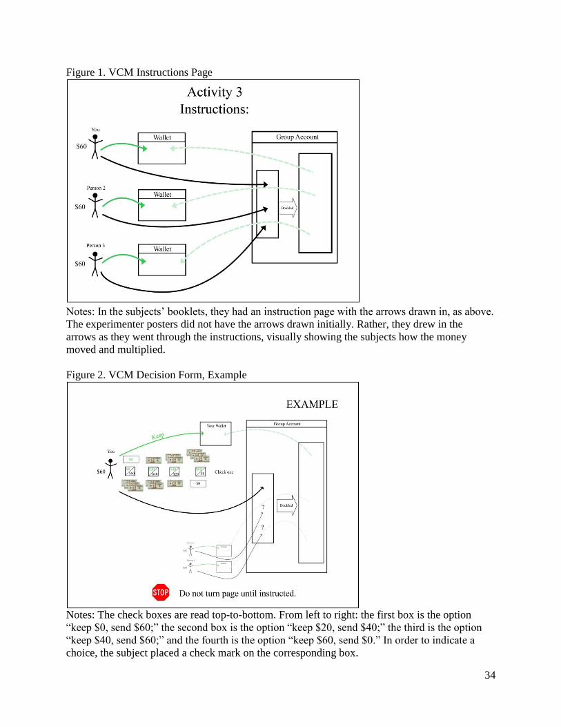
the instructions for both games is available in Appendix B. Figures 1 and 2 show the pictorial
representation of the instructions and the decision form for the VCM. Note that we are using the
more concrete “wallet” rather than the more abstract “private account” language – This was done
in the interest of clarity.
[Insert figures 1 & 2]
The arrows on the instructions page show the money starting at the person, and then
going into either the wallet and/or group account. All of the money in the group account is
doubled, and then split evenly between all three people, no matter what they choose to do.
Subjects then go through a series of examples, including the Nash Equilibrium, the Social
Optimum, and an intermediate case where every person does something different.
The decision form is just a modification of the instructions page. The decision maker has
been enlarged and given some choice options. The other two players have been shrunk down, so
as to make them less dominant, something that cannot be influenced, but still present.
Subjects had one of four possible choices: Keep $0/Send$60, Keep $20/Send$40,
Keep$40/Send$20, or $Keep $60/Send$0. To mark their choice, the subject just placed a check
mark on the box corresponding to their most preferred option. This simplification of the choice
space was necessary to have a visual representation, using money, without making the page too
cluttered and overwhelming. However, this our results may be understated because of the small
and discrete choice space.
Figure 3 and 4 present the instructions page and the example decision form for the
Donations experiments. Note that the form is similar to the VCM, except that now all of the

8
doubled dollars in the group account are donated to an organization rather than being split evenly
between the players.
[Insert Figures 3 & 4]
Similarly, subjects have the same four options, and select their choice by putting a
checkmark on the corresponding box.
c. Implementation Details
Data for this study come from the Preferences and Poverty Traps project, which is
described de Oliveira, Croson and Eckel (2009) and Croson et al (2010). We recruited 712
subjects from three communities (two low-income, N1 and N2, and one middle-income, N3) in
Dallas, Texas and a convenience sample of university undergraduates. To address the research
question of interest, we restrict the sample for this study to focus on the 571 self-identified
African-American and Hispanic subjects in the communities, of which 228 completed the
protocol in Spanish (instructions and booklets). Participants were recruited using flyers at homes,
local businesses and community centers as well as by recruiters hired to work in the community.
Participants arrived at a separate, local site for each community.
Sessions were run between June 2007 and August 2008 in either English or Spanish.
Individuals could participate only once. The 2-3 hour protocol included experimental tasks to
measure preferences (in order) for risk (Eckel and Grossman 2002, 2008), time (similar to Eckel,
Johnson and Montmarquette 2005) and cooperation (using a VCM, Ledyard 1995), as well as
willingness to provide local public goods, in this case charitable contributions to providers of
health, children’s education and job training in the community. The VCM always preceded the
Donations experiments, but the order of the charities was randomized. The risk and time games
9
are described in more detail in Croson et al (2010), and the VCM and Donations experiments are
described in more detail above. One of these six experimental tasks was chosen randomly for
payment, with no feedback between tasks.
After the experimental tasks were completed, beliefs about how much the other members
of their group would contribute to the group account for the VCM and to the charities were
elicited. Subjects then completed a series of social network, perception, and socio-demographic
surveys. Average earnings were $59.90, paid in private at the end of the session plus a $20 show-
up fee paid upon arrival.7
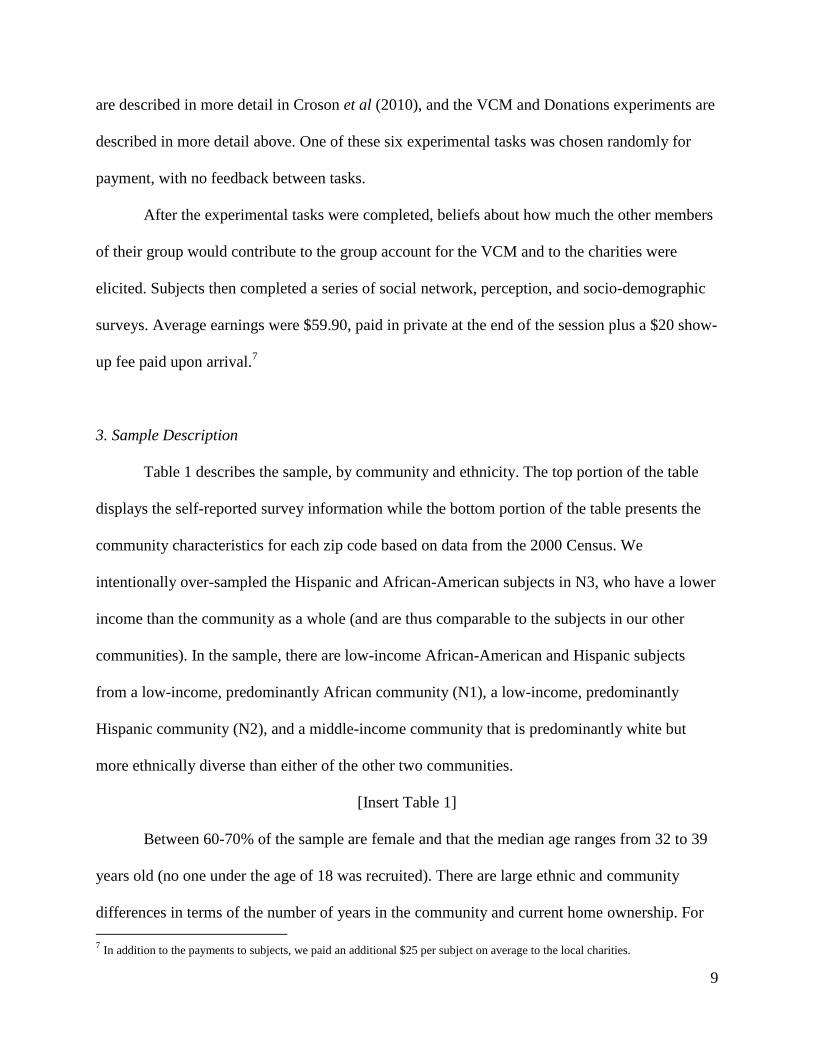
3. Sample Description
Table 1 describes the sample, by community and ethnicity. The top portion of the table
displays the self-reported survey information while the bottom portion of the table presents the
community characteristics for each zip code based on data from the 2000 Census. We
intentionally over-sampled the Hispanic and African-American subjects in N3, who have a lower
income than the community as a whole (and are thus comparable to the subjects in our other
communities). In the sample, there are low-income African-American and Hispanic subjects
from a low-income, predominantly African community (N1), a low-income, predominantly
Hispanic community (N2), and a middle-income community that is predominantly white but
more ethnically diverse than either of the other two communities.
[Insert Table 1]
Between 60-70% of the sample are female and that the median age ranges from 32 to 39
years old (no one under the age of 18 was recruited). There are large ethnic and community
differences in terms of the number of years in the community and current home ownership. For
7 In addition to the payments to subjects, we paid an additional $25 per subject on average to the local charities.

10
N1 and N3, the ethnic differences for the years in the community are highly significant (t-test,
p<0.001) whereas this difference is only marginal for N2 (t-test, p=0.08). Pooling across
ethnicities, there are significantly different tenures in the communities (t-test, all p<0.05), though
this is mainly due to different proportions of immigrants. There is a significantly higher
proportion of home ownership among Hispanics in N2 (proportions test, p<0.001), though the
other within-community differences are not statistically significant (proportions test, both
p>0.10). A smaller portion of the subjects from N1 are homeowners (proportions test, both
p<0.01) and there is no statistical difference between the proportion of homeowners in our
sample between N2 and N3. We also see large differences in terms of marriage rates across the
ethnicities, with 50-70% of the Hispanic sample reporting that they are married versus 15-17%
of the African-American sample (proportions test for each community, all p<0.001).
Turning to employment status, there are some interesting, though not altogether
surprising, differences at the community level. There are higher rates of full-time employment in
N3 (proportions test, both p<0.05) while N1 and N2 look very similar to each other (proportions
test, p=0.25) and there are no ethnic differences within the communities (proportions test, all
p>0.3). The proportion of subjects reporting that they have been unemployed in the last year is
similar across all three communities (a higher proportion in N1 than N2, p=0.006, but no
differences between N1 and N3, p=0.40, or N2 and N3, p=0.27, proportions tests). Additionally,
there are no significant differences in rates of job hunting (proportions test, all p>0.10) and part
time work (proportions test, all p>0.6).
Although subjects from all three of our communities have low levels of education, the
Hispanic subjects in all three communities have extremely low rates of completing high school,
ranging from 15–32%. There are higher rates of college attendance and graduation among the

11
African-American subjects (attendance 8.6% versus 30.6%, p=0.00; graduation 5.1% versus
9.2%, p=0.056, proportions tests).
4. Descriptive Results
We next turn to the descriptive results from the experimental tasks. We begin by
discussing differences in the proportion of the populations that contribute to the local public
goods before turning to the level of provision. We will then discuss the differences between
actual behavior and beliefs before turning to the econometric analysis.
a. Proportion of Contributors
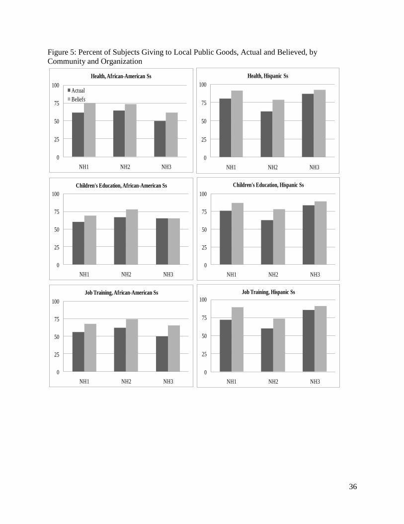
Figure 5 shows the percent of subjects who choose to contribute each of the local public
goods, by community and ethnicity. Columns 1, 2 and 3 present results for N1, N2 and N3
respectively. The top row presents the results for the health public good, the middle row is
children’s education, and the bottom row is job training.
[Insert Figure 5]
For N2 there are no differences between the proportion of African-American and
Hispanic subjects contributing to any of the three local public goods (proportions test, all
p>0.45). For N1 and N3, Hispanic subjects are significantly more likely to contribute toward
these goods (proportions test, N1, all p≤0.05; N3, p<0.001 for health and job training and p<0.10
for children’s education). There are no significant differences across communities for any of the
three local public goods for the African-American sample (proportions tests, all p>0.18).
However, the proportion of Hispanics who choose to provide these public goods does
vary significantly by community. This proportion is smallest in N2, which is the only community
in the sample that has Hispanics as the largest ethnic group in the community. The proportion of

12
Hispanic contributors in N1 and N3 is generally not significantly different (proportions test,
p>0.34 for health and children’s education, p=0.09 for job training). The proportion of
contributors are higher in N1 than N2 for the health public good (proportions test, p<0.05),
marginally higher for the children’s education (proportions test, p=0.08) and not significantly
different for job training (proportions test, p=0.13); whereas the proportion of contributors in N3
is always higher than the proportion in N2 (proportions test, all p<0.01). This seems to indicate
that the Hispanic population in the sample is responsive to community characteristics when
deciding whether to contribute. Further, it indicates that we have the best chance at estimating
the impacts of ethnicity and heterogeneity for the Health charity, since it has the most variation.
b. Amount Contributed
We next turn to the level of provision. Table 2 provides an overview of the contributions
to the lab VCM, the local health, children’s education, and job training public goods for each
community and ethnicity. Based on our previous work (de Oliveira, Croson and Eckel 2009), we
will use the VCM in our econometric analysis as a measure of the individual’s cooperative
preferences, in this case, their willingness to cooperate with their neighbors. We will discuss it
briefly here for clarity. Individuals had a $60 endowment to allocate between either their private
or public account. Anything placed in the private account was kept. Anything placed in the
public account was doubled. For the VCM, this doubled amount was then split evenly between
the three group members, regardless of the provision choice made. For the local public goods,
this doubled amount was sent to the local charity.8
8 Again, only one experimental task was chosen for payment, randomly and at the end of the session. There was no feedback
between tasks, and subjects only received feedback about the activity that was chosen for payment at the end of the session when
they were being paid individually, in private. Descriptions of all three organizations were read aloud before any of the local
public good decisions were made in order to minimize any potential order effects.
13
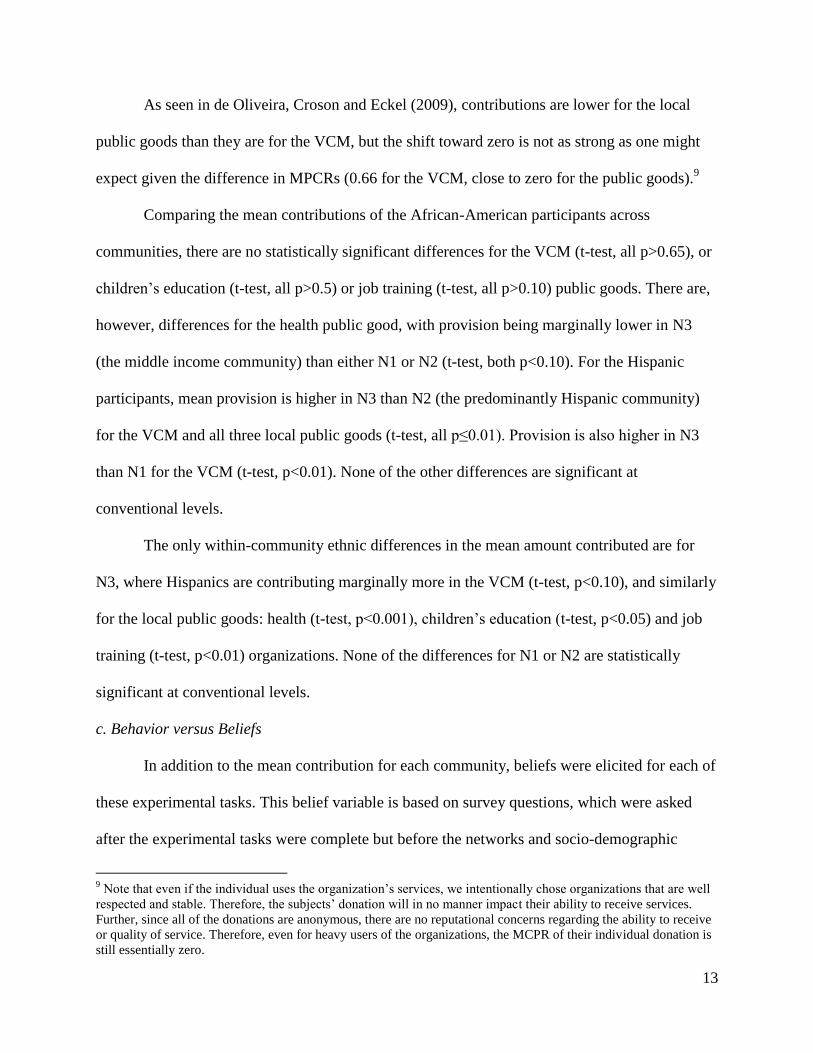
As seen in de Oliveira, Croson and Eckel (2009), contributions are lower for the local
public goods than they are for the VCM, but the shift toward zero is not as strong as one might
expect given the difference in MPCRs (0.66 for the VCM, close to zero for the public goods).9
Comparing the mean contributions of the African-American participants across
communities, there are no statistically significant differences for the VCM (t-test, all p>0.65), or
children’s education (t-test, all p>0.5) or job training (t-test, all p>0.10) public goods. There are,
however, differences for the health public good, with provision being marginally lower in N3
(the middle income community) than either N1 or N2 (t-test, both p<0.10). For the Hispanic
participants, mean provision is higher in N3 than N2 (the predominantly Hispanic community)
for the VCM and all three local public goods (t-test, all p≤0.01). Provision is also higher in N3
than N1 for the VCM (t-test, p<0.01). None of the other differences are significant at
conventional levels.
The only within-community ethnic differences in the mean amount contributed are for
N3, where Hispanics are contributing marginally more in the VCM (t-test, p<0.10), and similarly
for the local public goods: health (t-test, p<0.001), children’s education (t-test, p<0.05) and job
training (t-test, p<0.01) organizations. None of the differences for N1 or N2 are statistically
significant at conventional levels.
c. Behavior versus Beliefs
In addition to the mean contribution for each community, beliefs were elicited for each of
these experimental tasks. This belief variable is based on survey questions, which were asked
after the experimental tasks were complete but before the networks and socio-demographic
9 Note that even if the individual uses the organization’s services, we intentionally chose organizations that are well
respected and stable. Therefore, the subjects’ donation will in no manner impact their ability to receive services.
Further, since all of the donations are anonymous, there are no reputational concerns regarding the ability to receive
or quality of service. Therefore, even for heavy users of the organizations, the MCPR of their individual donation is
still essentially zero.

14
surveys began (or any feedback was received). For the VCM, participants were asked: “Think
back to Activity 3 where you and two other people made a decision about how much to keep and
how much to donate to the group. The money donated was doubled and then split evenly among
you. How much money do you think the other two people donated? Check ONE for EACH
person,” with possible responses of $0, $20, $40 or $60. For the local public goods, participants
were asked: “Think back to [insert activity number] where you and two other people made a
decision about how much to keep and how much to donate to the group. The money was doubled
and then donated to [insert organization’s name here]. How much money do you think the other
two people donated? Check ONE for EACH person,” again with possible responses of $0, $20,
$40 or $60. Since subjects answered this question for each of their two group members,
responses are averaged to get the belief variable that used in this analysis.
Comparing the believed and actual contributions for the same population and item,
beliefs are never significantly less than actual contributions. Thus participants were either well-
calibrated or optimistic about others’ contributions. In N1, beliefs are greater than actual
contributions for Hispanics in the VCM (t-test, p=0.02), for both the African-American and
Hispanic subjects for health (t-test, both p<0.05) and job training public goods (t-test, both
p<0.05), and marginally for the children’s education (t-test, both p<0.10).
Additionally, beliefs are greater than contributions for the Hispanic sample in N2 for all
three of the local public goods (t-test, all p<0.01) but not for the VCM. All other comparisons are
not statistically significant (t-test, all p>0.15).
When comparing beliefs for each ethnic group within a community for the VCM,
Hispanics hold higher beliefs than African-Americans in N1 (t-test, p<0.05) but not for the other
two communities (t-test, both p>0.15). This same relationship holds for the health (t-test, N1,
15
p<0.05; N2, p<0.10; N3, p<0.001), and for the children’s education (t-test, p<0.05) and job
training organizations (t-test, p<0.01) in N3 only (t-test, all other p>0.15).
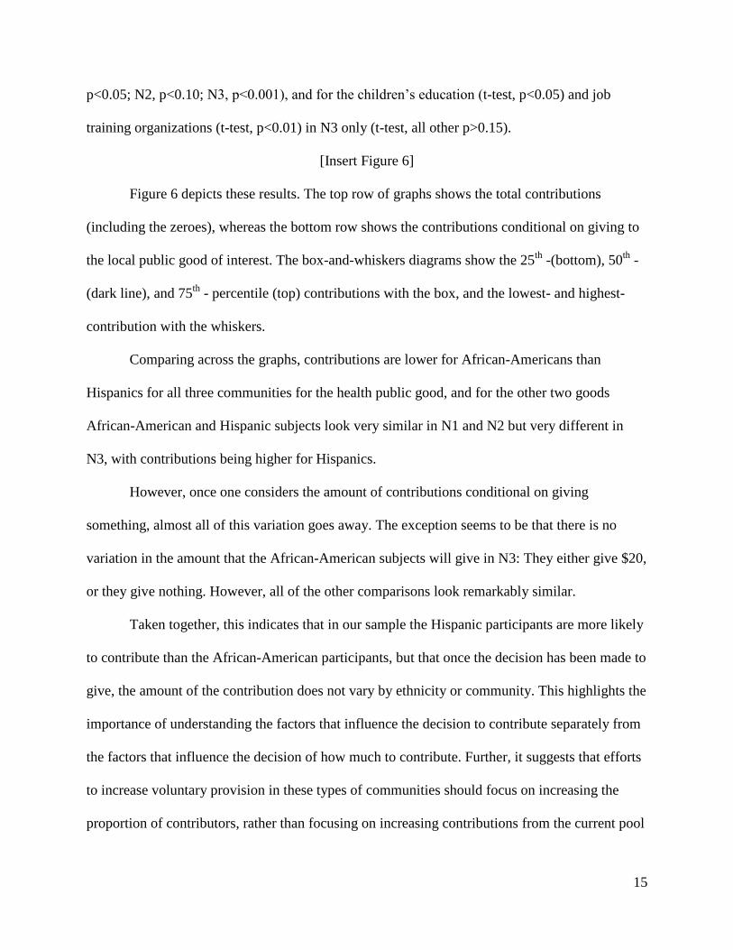
[Insert Figure 6]
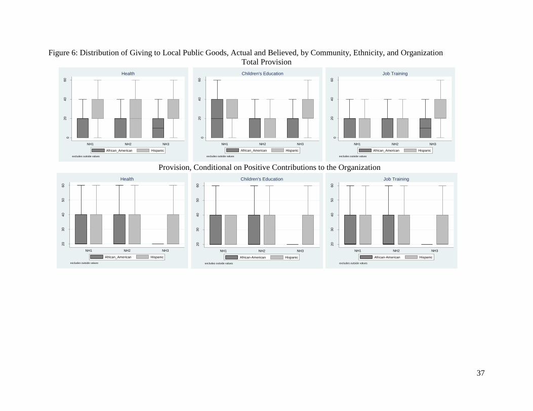
Figure 6 depicts these results. The top row of graphs shows the total contributions
(including the zeroes), whereas the bottom row shows the contributions conditional on giving to
the local public good of interest. The box-and-whiskers diagrams show the 25th
-(bottom), 50th
-
(dark line), and 75th
- percentile (top) contributions with the box, and the lowest- and highest-
contribution with the whiskers.
Comparing across the graphs, contributions are lower for African-Americans than
Hispanics for all three communities for the health public good, and for the other two goods
African-American and Hispanic subjects look very similar in N1 and N2 but very different in
N3, with contributions being higher for Hispanics.
However, once one considers the amount of contributions conditional on giving
something, almost all of this variation goes away. The exception seems to be that there is no
variation in the amount that the African-American subjects will give in N3: They either give $20,
or they give nothing. However, all of the other comparisons look remarkably similar.
Taken together, this indicates that in our sample the Hispanic participants are more likely
to contribute than the African-American participants, but that once the decision has been made to
give, the amount of the contribution does not vary by ethnicity or community. This highlights the
importance of understanding the factors that influence the decision to contribute separately from
the factors that influence the decision of how much to contribute. Further, it suggests that efforts
to increase voluntary provision in these types of communities should focus on increasing the
proportion of contributors, rather than focusing on increasing contributions from the current pool

16
of contributors, though additional studies are required to test the robustness of this result across
other communities and ethnic groups. We now turn to the econometric analysis to further
investigate this issue.
5. Likelihood of Contributing
Since our descriptive results indicate that most of the action will be on the decision to
contribute, we examine the determinants of the likelihood of contributing to these local public
goods.10
We begin by modeling the likelihood of contributing to each organization as a function of
ethnicity and our community-heterogeneity variables, as shown in Table 3. For our base models,
we include ethnicity and whether or not an individual is in the ethnic majority of their
neighborhood as well as one of our three measures of heterogeneity. The first is the traditional
ethnic fractionalization index, which is employed by the majority of the literature. This variable
takes on a (theoretical) value of one for perfectly heterogeneous communities and a value of zero
for perfectly homogeneous communities.11
The second measure is ethnic polarization, a key
variable in the ethnic conflict literature (see e.g. Montavalo and Reynal-Querol 2005; Reynal-
Querol 2002). In this literature, the (½, 0, 0, …, 0, ½) distribution is the one thought to product
the most conflict, so this variable measures how far a population is from a 50/50 split. It takes on
a value of 1 if the population has two groups, each comprising 50% of the distribution, and the
value decreases toward zero as the population becomes less polarized. The third heterogeneity
measure is an interaction effect between being a member of our two main ethnic groups and the
10
Since we have a sample of volunteers, we focus on the direction and significance of impacts rather than their
magnitudes per se. 11
Shares of the population are taken from the 2000 census for each zip code.
17
percentage of your co-ethnics in your neighborhood.12
These interaction effects are meant to
capture the idea that different ethnic groups may have an asymmetric response to the distribution
of ethnic groups in their community.
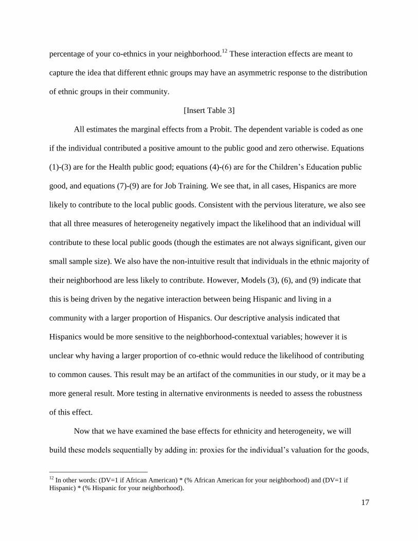
[Insert Table 3]
All estimates the marginal effects from a Probit. The dependent variable is coded as one
if the individual contributed a positive amount to the public good and zero otherwise. Equations
(1)-(3) are for the Health public good; equations (4)-(6) are for the Children’s Education public
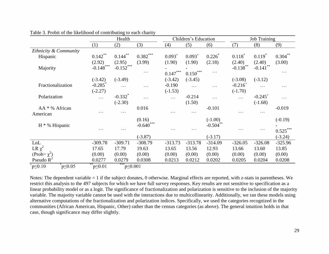
good, and equations (7)-(9) are for Job Training. We see that, in all cases, Hispanics are more
likely to contribute to the local public goods. Consistent with the pervious literature, we also see
that all three measures of heterogeneity negatively impact the likelihood that an individual will
contribute to these local public goods (though the estimates are not always significant, given our
small sample size). We also have the non-intuitive result that individuals in the ethnic majority of
their neighborhood are less likely to contribute. However, Models (3), (6), and (9) indicate that
this is being driven by the negative interaction between being Hispanic and living in a
community with a larger proportion of Hispanics. Our descriptive analysis indicated that
Hispanics would be more sensitive to the neighborhood-contextual variables; however it is
unclear why having a larger proportion of co-ethnic would reduce the likelihood of contributing
to common causes. This result may be an artifact of the communities in our study, or it may be a
more general result. More testing in alternative environments is needed to assess the robustness
of this effect.
Now that we have examined the base effects for ethnicity and heterogeneity, we will
build these models sequentially by adding in: proxies for the individual’s valuation for the goods,
12
In other words: (DV=1 if African American) * (% African American for your neighborhood) and (DV=1 if
Hispanic) * (% Hispanic for your neighborhood).

18
socio-demographics, perceptions of neighbors, preference measures (from the experimental
data), and beliefs about whether or not anyone else in the subject’s experimental group would
donate to the organization. These results are presented in Table 4, panels a (for Health), b (for
Children’s Education) and c (for Job Training).13
[Insert Table 4]
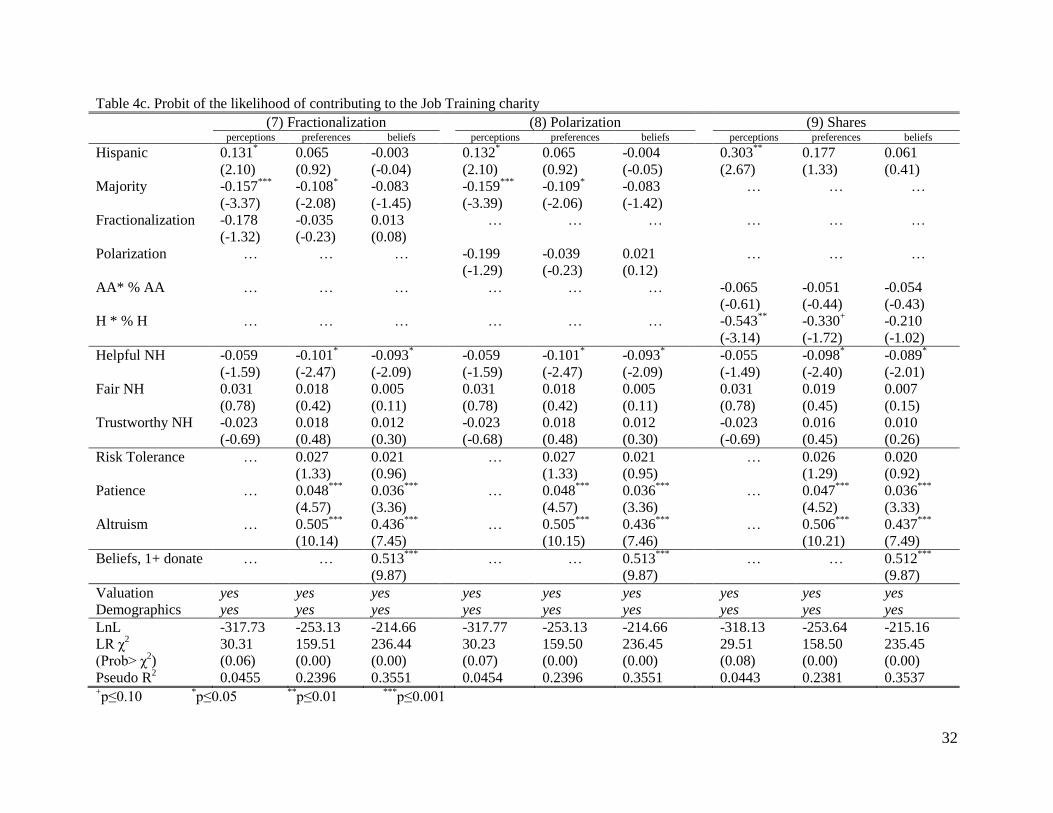
The main result from adding this richer set of perception and preference variables to the
model is that, with the exception of the negative interaction between being Hispanic and the
percentage of Hispanics in your community, the heterogeneity measures are no longer even
approaching statistical significance. We believe this indicates that the negative impact of
Fractionalization or Polarization previously found in the literature may just be serving as a proxy
for differences in perceptions, preferences, and beliefs. If true, this is positive news for policy
makers who cannot force communities to become more homogeneous, but may be able to impact
the other dimensions. We will now briefly discuss some of the interesting effects found in this
richer variable set before going on to the concluding discussion.
The first sets of variables added to the models are the “perception” variables. These
questions are adapted from the World Values Survey (WVS) and measure how helpful, fair, and
trustworthy you believe your neighbors are. We see that individuals view helpful neighbors are a
substitute for their own contributions: If you believe people in your neighborhood are very
helpful you are less likely to contribute to neighborhood causes. We do not see a relationship
between the perception that your neighbors are fair and your likelihood of contributing, and the
relationship between trust and likelihood of giving is positive but not very robust.
13
In the interest of brevity, the estimates of the “valuation” and demographic variables have been suppressed. A full
list of the variables in available in the footnote to the table, and the estimates are available in the supplement to this
paper upon request from the authors.
19
The second sets of variables added to the models are the “preferences” variables: Risk
tolerance, patience, and altruism or cooperation. We see a strong impact of the preference
variables on the likelihood of giving. The risk and patience measures are discussed in more detail
in Croson et al (2010), but will be summarized here for clarity. The risk measure is a version of
the one put forward by Eckel and Grossman (2002, 2008). Subjects see a series of 50/50 gambles
that begin with a sure thing of $80 (coded 1) and then increase an risk and return space up to an
expected value maximizing point ($0 / $240, coded 5) and continue to increase in standard
deviation while holding the expected value constant (-$20 / $260, coded 6). Therefore, higher
numbers of this variable indicate than an individual is more risk tolerant.14
We hypothesized that
contributing to neighborhood public goods might be a risky decision, since you may never
benefit from the organization’s services. However, we do not see a relationship between risk
tolerance and the likelihood of contributing.
The patience measure is similar to the one in Eckel, Johnson and Montmarquette, (2005).
Subjects make a series of choices between smaller and sooner (SS) and larger and later (LL)
options. The SS payment is always $60 tomorrow. The LL payment varies by waiting time (1
month or 5 months) and annual simple interest rate (20-160%).15
Patience is defined as the total
number of times and individual is willing to wait for the LL payoff. We hypothesized that more
patient individuals would be more likely to contribute to the local public goods, since the
contributions are an investment in their community – an investment that will take time to pay off.
14
In Croson et al (2010), we found that there no significant difference between communities, gender, or ethnicity in
terms of the average gamble choice or the distribution of observed choices. 15
Though there is not a significant difference in the mean number of patient choices, there is a substantial difference
in terms of the proportion of subjects who are willing to wait for the LL payoff, with N3 exhibiting the highest
willingness to wait and Hispanics being significantly more willing to wait (almost 70% of African-Americans refuse
to ever wait for the LL payoff versus only 50% of Hispanics; Croson et al 2010).
20
We see a very strong and robust relationship between patience and contributions for the Health
and Job Training public goods, and a smaller/less robust relationship for Children’s Education.
Our third preference measure comes from the VCM contributions, and is meant to proxy
an individual’s altruism or willingness to cooperate with their neighbors, as previously described
and as seen in de Oliveira, Croson and Eckel (2009). The VCM is a discrete ($0, $20, $40, $60)
choice, with groups of size of 3 and MPCR=0.66. Since we are examining the likelihood of
contributing to the local public goods, we construct a variable equal to one if the subject
contributed to the VCM group account and zero otherwise. We hypothesized that more altruistic
individuals would be more likely to contribute to the public goods, as is confirmed by the results.
The final variable added is whether or not an individual believes that any of the others in
their group will choose to contribute to the local public goods.16
We see a strong positive
relationship between beliefs and behavior, even controlling for preferences and demographics.
Further, we see that once preferences and beliefs are controlled for, the Hispanic main effect is
no longer statistically significant. However, the Hispanic*%Hispanic interaction is (generally)
still statistically significant. This suggests that the observed differences between the ethnicities
and communities in our sample are largely driven by differences in preferences and beliefs
between the populations, with some of the effect still coming though the greater sensitivity of
Hispanics to their relative size in the community.
6. Closing Comments
The current economic reality is a world of tightening government budgets with a
simultaneous increase in the need of government services. It is becoming increasingly difficult
16
Again, only one experimental task was chosen for payment, randomly and at the end of the session. There was no feedback
between tasks, and subjects only received feedback about the activity that was chosen for payment at the end of the session when
they were being paid individually, in private.

21
for city and state governments to provide services and public goods that are essential for quality
of life and local economic growth, particularly in low-income communities. At the same time,
these communities are becoming ever-more diverse. Unfortunately, previous research suggests
that this increased diversity will make the provision of these services more difficult, even as they
are needed most (see e.g. Alesina and La Ferrara 2000; Alesina, Baqir and Easterly 1999). In
order to understand and address this disconnect between the need for public services and the
ability of governments to provide them, it is important to understand the impacts of both
individual characteristics and community characteristics (including this diversity) on public good
provision and to investigate alternative funding sources, such as the voluntary provision (by
residents) of these local public goods.
To investigate potential avenues for increasing voluntary provision of local public goods,
and to examine the impacts of ethnicity and heterogeneity on individual decision making, we
conducted a field experiment with a new (to experimental economics) and policy relevant
sample, low-income Hispanic and African-American subjects.
We begin by confirming the negative impact of heterogeneity on voluntary provision of
local public goods, and then examine a richer set of variables not generally considered in this
literature due to the data limitations inherent in large-scale survey data. We complement existing
studies by focusing on a small number of communities and subjects (reducing the breadth of the
study), but collecting a wealth of information not typically available to the econometrician
(increasing depth).
We find that, once preferences and beliefs have been taken into account neither the ethnic
fractionalization nor polarization indices are statistically significant. A somewhat more crude
22
measure, an interaction between your own ethnicity and the share of co-ethnics in your
community remains (generally) statistically significant.
Taking the evidence together seems to indicate that the observed differences between
communities and the African-Americans and Hispanics in our sample are largely driven by
differences in preferences and beliefs across the two populations. However, as observed in the
descriptive analysis, the beliefs people hold are not correct. Exactly why these beliefs are over-
optimistic and how they are sustainable is an interesting question for future research.
In all, the results suggest that policies aimed at changing individuals’ beliefs about the
potential contribution behavior of their neighbors is likely to substantially impact the individual
willingness to voluntarily provide local public goods. Additionally, these results suggest that
policies that either impact individual’s willingness to delay instant gratification or, at minimum,
take into account that discount rates may vary by culture, will have a greater probability of
success when it comes to encouraging the voluntary provision of local public goods. Additional
studies are needed to test the robustness and generality of these results for policy analysis. This is
especially important in a world of ever-tightening governments and increasing diversity. As
diversity increases, provision preferences change. Additionally, city and state governments are
less able to fund these quality-of-life public goods. Finding ways to increase voluntary provision
of important services, while allowing diverse communities to have the power to support the
services that they value, may help alleviate some of the current tension between the need for
these vital public goods and the lack of government funding.

23
References:
Alesina, Alberto, Reza Baqir and William Easterly. 1999. “Public Goods and Ethnic Divisions.”
Quarterly Journal of Economics. 114.4: 1243-1284.
Alesina, Alberto and Eliana La Ferrara. 2005. “Ethnic Diversity and Economic Performance.”
Journal of Economic Literature. 43: 762-800.
Alesina, Alberto and Eliana La Ferrara. 2000. “Participation in Heterogeneous Communities.”
Quarterly Journal of Economics. 115.3: 847-904.
Banerjee, Abhijit, Lakshmi Iyer and Rohini Somanathan. 2005. “History, Social Divisions, and
Public Goods in Rural India.” Journal of the European Economic Association. 3.2-3:
639-647.
Clark, Jeremy and Bonggeun Kim. 2009. “The Effect of Neighorhood Diverity on Volunteering:
Evidence from New Zeland.” Working paper.
Costa, Dora L. and Matthew E. Kahn. 2003. “Civic Engagement and Community Heterogeneity:
An Economist’s Perspective.” Perspectives on Politics. 1.1: 103-111.
Croson, Rachel T. A., Angela C. M. de Oliveira, Catherine Eckel, Philip J. Grossman, Cathleen
Johnson, Sherry Xin Li. 2010. “Preferences for Risk and Time among Low-Income
Minorities.” Working Paper.
de Oliveira, Angela C. M., Rachel T. A. Croson and Catherine Eckel. 2009. “Are Preferences
Stable Across Domains? An Experimental Investigation of Social Preferences in the
Field.” CBEES Working Paper #2008-3.
Easterly, William and Ross Levine. 1997. “Africa’s Growth Tragedy: Policies and Ethnic
Divisions.” Quarterly Journal of Economics. 112.4: 1203-1250.

24
Eckel, Catherine and Philip J. Grossman. 2008. “Forecasting Risk Attitudes: An Experimental
Study Using Actual and Forecast Gamble Choices.” Journal of Economic Behavior and
Organization. 68.1: 1-17.
Eckel, Catherine and Philip J. Grossman. 2002. “Sex Differences and Statistical Stereotyping in
Attitudes Toward Financial Risk.” Evolution and Human Behavior. 23.4: 281-295.
Eckel, Catherine, Cathleen A. Johnson and Claude Montmarquette. 2005. “Saving Decisions of
the Working Poor: Short- and Long-term Horizons.” Research in Experimental
Economics, Volume 10: Field Experiments in Economics. Edited by Jeff Carpenter,
Glenn W. Harrison, and John A. List. Greenwich, CT: JAI Press: 219-260.
Gaibulloev, Khusrav and James Murdoch. 2007. “Impact of Fractionalization on the Provision of
International Public Goods: The Case of National Defense.” Working Paper.
Habyarimana, James, Macartan Humphreys, Daniel N. Posner, and Jeremy M. Weinstein. 2007.
“Why Does Ethnic Diversity Undermine Public Goods Provision?” American Political
Science Review. 101.4: 709-725.
Ledyard, John. 1995. “Public Goods: A Survey of Experimental Research”, in: Handbook of
Experimental Economics, ed. by John Kagel and Alvin Roth, Princeton University Press.
Miguel, Edward. 2001. “Ethnic diversity and school funding in Kenya.” UC-Berkeley CIDER
WP #C01-119.
Miguel, Edward and Mary Kay Gugerty. 2005. “Ethnic Diversity, Social Sanctions, and Public
Goods in Kenya.” Journal of Public Economics. 89.11-12: 2325-2368.
Montalvo, José G. and Marta Reynal-Querol. 2005. “Ethnic Polarization, Potential Conflict, and
Civil Wars.” American Economic Review. 95.3: 796-816.
25
Reynal-Querol, Marta. 2002. “Ethnicity, Political Systems, and Civil wars.” Journal of Conflict
Resolution. 46.1: 29-54.
Vigdor, Jacob L. 2004. “Community Composition and Collective Action: Analyzing Initial Mail
Response to the 2000 Census.” Review of Economics and Statistics. 86.1: 303-312.

26
Table 1: Sample & Community Descriptions
Variable
N 1 N2 N3
African-
American
Hispanic African-
American
Hispanic African-
American
Hispanic
Sample Characteristics, N 186 46 82 176 26 55
Demographics
Female, % 60.75 69.57 69.51 62.29 69.23 68.52
Foreign Born, % 1.09 91.30 0.00 63.95 0.00 90.91
Median Age, in years 39 32 39 37 36.5 32
Kids in HH 1.25 2.39 1.84 1.70 1.08 2.48
Years in NH 17.6 7.53 23.52 19.59 17.06 8.42
Home Owner, % 15.93 6.52 20.25 43.10 38.46 25.45
Religious, 1+/week, % 51.08 43.48 50.00 49.43 61.54 67.27
Marital Status, % a
Single 57.53 15.22 65.85 28.98 53.85 5.45
Married 16.13 73.91 17.07 52.27 15.38 72.73
Divorced 20.97 10.87 14.63 10.80 26.92 16.36
Widow 4.84 0.00 2.44 7.39 3.85 5.45
Employment, % a
FT Job 20.21 19.57 15.85 17.61 38.46 29.09
PT Job 9.68 13.04 9.76 12.50 7.69 12.73
Temp Job 33.87 19.57 24.39 22.16 19.23 23.64
Retired 4.84 0.00 3.66 8.52 7.69 3.64
No Job 34.95 47.83 50.00 47.73 34.62 34.55
Job Hunting 33.33 15.22 30.49 21.59 34.62 14.55
Unemployed in last year 60.75 48.89 57.32 40.80 57.69 50.91
Education, % a
HS Dropout (or less) 23.66 84.78 34.15 67.61 7.69 70.91
HS Grad 33.87 6.52 36.59 11.93 30.77 16.36
Some College 31.72 4.35 24.39 10.80 42.31 5.45
College Grad (or more) 10.22 2.17 3.66 5.11 19.23 7.27

27
Table 1, Continued
Variable
N 1 N2 N3
African-
American
Hispanic African-
American
Hispanic African-
American
Hispanic
Sample Characteristics, N 186 46 82 176 26 55
Session
Spanish Book, % 0.00 95.65 0.00 75.57 0.00 92.73
# Ss Know 1.03 4.55 1.65 2.85 2.58 1.15
# Ss Recognize 1.37 6.45 2.63 3.50 3.36 1.68
Community Characteristics b
N, Zip Code 18,731 22,173 37,371
Female, % 52.8 50.9 48.5
African-American, % 85.3 34.2 8.1
Hispanic, % 11.8 62.1 27.4
Foreign Born, % 7.7 24.9 21.9
Median Age 34.4 24.9 31.2
Median HH Income 16,043 22,555 54,000
Median Per Capita Income 9,411 8,534 23,040
Labor Force Participation, % 47.0 47.7 75.3
Families < Poverty Level, % 39.2 34.9 6.9
High School Grad +, % 53.6 34.3 79.5
College Grad +, % 6.4 2.3 27.9 a Results may not sum to 100 due to rounding and/or because categories are not mutually exclusive
b Community data from the 2000 Census, zip codes 75215, 75212, 75074 respectively.

28
Table 2: Mean Provision and Beliefs by Community and Ethnicity, VCM and Charities, in Dollars
VCM Health Children’s Education Job Training
Population
µ
(Std. dev) Belief
µ
(Std. dev) Belief
µ
(Std. dev) Belief
µ
(Std. dev) Belief
N1
African-
American
24.9 24.2 18.3 21.5 18.6 21.2 16.3 20.4
(20.9) (18.9) (18.3) (17.9) (18.7) (19.0) (17.4) (18.7)
Hispanic 23.5 30.7 23.0 28.5 21.3 25.4 19.6 24.6
(17.0) (16.1) (15.8) (14.9) (14.8) (15.9) (15.5) (14.7)
N2
African-
American
25.4 25.1 17.8 19.9 19.3 21.6 18.0 19.8
(19.6) (19.4) (16.6) (16.8) (17.1) (17.1) (17.9) (16.1)
Hispanic 26.3 28.3 19.3 24.3 17.1 21.7 16.4 20.8
(22.1) (18.0) (18.6) (18.2) (16.6) (16.7) (16.5) (17.5)
N3
African-
American
26.9 29.6 11.5 15.4 16.9 17.7 12.3 15
(21.9) (21.8) (12.9) (15.6) (15.7) (16.8) (15.0) (15.6)
Hispanic 35.6 33.5 26.5 28.7 26.2 28.2 23.3 26.1
(20.3) (17.6) (15.9) (15.2) (17.2) (16.9) (14.3) (14.8)
29
Table 3. Probit of the likelihood of contributing to each charity
Health Children’s Education Job Training
(1) (2) (3) (4) (5) (6) (7) (8) (9)
Ethnicity & Community
Hispanic 0.142**
0.144**
0.382***
0.093+ 0.093
+ 0.226
* 0.118
* 0.119
* 0.304
**
(2.92) (2.95) (3.99) (1.90) (1.90) (2.18) (2.40) (2.40) (3.00)
Majority -0.148***
-0.152***
…
-
0.147***
-
0.150***
…
-0.138**
-0.141**
…
(-3.42) (-3.49) (-3.42) (-3.45) (-3.08) (-3.12)
Fractionalization -0.285* … … -0.190 … … -0.216
+ … …
(-2.27) (-1.53) (-1.70)
Polarization … -0.332* … … -0.214 … … -0.245
+ …
(-2.30) (1.50) (-1.68)
AA * % African
American … …
0.016 … …
-0.101 … …
-0.019
(0.16) (-1.00) (-0.19)
H * % Hispanic … …
-0.640***
… …
-0.504**
… …
-
0.525***
(-3.87) (-3.17) (-3.24)
LnL -309.78 -309.71 -308.79 -313.73 -313.78 -314.09 -326.05 -326.08 -325.96
LR χ2
(Prob> χ2)
17.65
(0.00)
17.79
(0.00)
19.63
(0.00)
13.65
(0.00)
13.56
(0.00)
12.93
(0.00)
13.66
(0.00)
13.60
(0.00)
13.85
(0.00)
Pseudo R2 0.0277 0.0279 0.0308 0.0213 0.0212 0.0202 0.0205 0.0204 0.0208
+p≤0.10
*p≤0.05
**p≤0.01
***p≤0.001
Notes: The dependent variable = 1 if the subject donates, 0 otherwise. Marginal effects are reported, with z-stats in parentheses. We
restrict this analysis to the 497 subjects for which we have full survey responses. Key results are not sensitive to specification as a
linear probability model or as a logit. The significance of fractionalization and polarization is sensitive to the inclusion of the majority
variable. The majority variable cannot be used with the interactions due to multicollinearity. Additionally, we ran these models using
alternative computations of the fractionalization and polarization indices. Specifically, we used the categories recognized in the
communities (African American, Hispanic, Other) rather than the census categories (as above). The general intuition holds in that
case, though significance may differ slightly.

30
Table 4a. Probit of the likelihood of contributing to the Health charity
(1) Fractionalization (2) Polarization (3) Shares perceptions preferences beliefs perceptions preferences beliefs perceptions preferences beliefs
Hispanic 0.214**
0.166* 0.091 0.0215
** 0.167
* 0.091 0.403
*** 0.316
** 0.178
(3.05) (2.16) (1.04) (3.05) (2.18) (1.05) (3.84) (2.62) (1.25)
Majority -0.198***
-0.169***
-0.183***
-0.201***
-0.171***
-0.184***
… … …
(-4.30) (-3.43) (-3.45) (-4.35) (-3.46) (-3.44)
Fractionalization -0.261* -0.156 -0.086 … … … … … …
(-1.96) (-1.10) (-0.56)
Polarization … … … -0.300* -0.185 -0.099 … … …
(-1.96) (-1.13) (-0.55)
AA * % AA … … … … … … -0.096 -0.111 -0.222+
(-0.84) (-0.91) (-1.67)
H * % H … … … … … … -0.713***
-0.578**
-0.529**
(-4.10) (-3.07) (-2.58)
Helpful NH -0.092* -0.130
*** -0.134
*** -0.092
* -0.130
*** -0.134
*** -0.090
* -0.128
*** -0.133
***
(-2.54) (-3.41) (-3.25) (-2.54) (-3.41) (-3.25) (-2.48) (-3.36) (-3.21)
Fair NH 0.013 0.00 0.010 0.013 0.000 0.010 0.013 0.001 0.010
(0.34) (0.01) (0.22) (0.33) (0.01) (0.22) (0.35) (0.03) (0.24)
Trustworthy NH 0.034 0.073* 0.061 0.034 0.073
* 0.061 0.033 0.072
* 0.059
(1.03) (2.09) (1.61) (1.04) (2.09) (1.61) (1.01) (2.06) (1.58)
Risk Tolerance … 0.023 0.024 … 0.023 0.024 … 0.023 0.024
(1.18) (1.17) (1.18) (1.17) (1.16) (1.18)
Patience … 0.049***
0.033**
… 0.049***
0.033**
… 0.049***
0.033**
(4.69) (3.06) (4.69) (3.06) (4.62) (3.02)
Altruism … 0.441 0.378***
… 0.442***
0.378***
… 0.444***
0.381***
(8.13)***
(6.18) (8.14) (6.18) (8.21) (6.24)
Beliefs, 1+ donate … … 0.545***
… … 0.545***
… … 0.543***
(9.75) (9.74) (9.69)
Valuation yes yes yes yes yes yes yes yes yes
Demographics yes yes yes yes yes yes yes yes yes
LnL -295.79 -239.78 -198.43 -295.79 -239.74 -198.43 -295.99 -240.02 -199.05
LR χ2
(Prob> χ2)
45.64
(0.00)
157.67
(0.00)
240.35
(0.00)
45.64
(0.00)
157.73
(0.00)
240.35
(0.00)
45.24
(0.00)
157.18
(0.00)
239.11
(0.00)
Pseudo R2 0.0716 0.2474 0.3772 0.0716 0.2475 0.3772 0.0710 0.2467 0.3752
+p≤0.10
*p≤0.05
**p≤0.01
***p≤0.001

31
Table 4b. Probit of the likelihood of contributing to the Children’s Education charity
(4) Fractionalization (5) Polarization (6) Shares perceptions preferences beliefs perceptions preferences beliefs perceptions preferences beliefs
Hispanic 0.054 0.010 -0.055 0.055 0.011 -0.055 0.200+ 0.104 0.020
(0.88) (0.15) (-0.76) (0.89) (0.16) (-0.76) (1.71) (0.80) (0.14)
Majority -0.165***
-0.135**
-0.138**
-0.168***
-0.136**
-0.139**
… … …
(-3.68) (-2.76) (-2.64) (-3.70) (-2.77) (-2.64)
Fractionalization -0.189 -0.103 -0.114 … … … … … …
(-1.44) (-0.73) (-0.75)
Polarization … … … -0.215 -0.119 -0.128 … … …
(-1.42) (-0.73) (-0.73)
AA* % AA … … … … … … -0.121 -0.128 -0.152
(-1.15) (-1.14) (-1.22)
H * % H … … … … … … -0.556***
-0.417* -0.412
*
(-3.28) (-2.27) (-2.12)
Helpful NH -0.104**
-0.146***
-0.147***
-0.104**
-0.146***
-0.147***
-0.101**
-0.144***
-0.145***
(-2.86) (-3.79) (-3.50) (-2.86) (-3.79) (-3.50) (-2.79) (-3.74) (-3.46)
Fair NH 0.014 0.009 0.003 0.014 0.009 0.003 0.014 0.009 0.003
(0.37) (0.22) (0.06) (0.37) (0.22) (0.06) (0.37) (0.23) (0.06)
Trustworthy NH 0.040 0.076* 0.094
** 0.040 0.076
* 0.094
** 0.039 0.075
* 0.093
*
(1.23) (2.22) (2.57) (1.23) (2.22) (2.57) (1.21) (2.19) (2.55)
Risk Tolerance … 0.007 -0.004 … 0.007 -0.004 … 0.007 -0.004
(0.38) (-0.21) (0.38) (-0.21) (0.37) (-0.21)
Patience … 0.028**
0.013 … 0.028**
0.013 … 0.028**
0.012
(2.95) (1.27) (2.95) (1.27) (2.92) (1.24)
Altruism … 0.463***
0.424***
… 0.463***
0.424***
… 0.464***
0.426***
(8.79) (7.13) (8.79) (7.13) (8.83) (7.17)
Beliefs, 1+ donate … … 0.541***
… … 0.541***
… … 0.542***
(10.18) (10.18) (10.20)
Valuation yes yes yes yes yes yes yes yes yes
Demographics yes yes yes yes yes yes yes yes yes
LnL -301.06 -253.43 -209.95 -301.08 -253.43 -209.97 -301.45 -253.73 -210.18
LR χ2
(Prob> χ2)
39.00
(0.01)
134.25
(0.00)
221.20
(0.00)
38.95
(0.01)
134.25
(0.00)
221.17
(0.00)
38.22
(0.01)
133.66
(0.00)
220.75
(0.00)
Pseudo R2 0.0608 0.2094 0.3450 0.0608 0.2094 0.3450 0.0596 0.2085 0.3443
+p≤0.10
*p≤0.05
**p≤0.01
***p≤0.001
32
Table 4c. Probit of the likelihood of contributing to the Job Training charity
(7) Fractionalization (8) Polarization (9) Shares perceptions preferences beliefs perceptions preferences beliefs perceptions preferences beliefs
Hispanic 0.131* 0.065 -0.003 0.132
* 0.065 -0.004 0.303
** 0.177 0.061
(2.10) (0.92) (-0.04) (2.10) (0.92) (-0.05) (2.67) (1.33) (0.41)
Majority -0.157***
-0.108* -0.083 -0.159
*** -0.109
* -0.083 … … …
(-3.37) (-2.08) (-1.45) (-3.39) (-2.06) (-1.42)
Fractionalization -0.178 -0.035 0.013 … … … … … …
(-1.32) (-0.23) (0.08)
Polarization … … … -0.199 -0.039 0.021 … … …
(-1.29) (-0.23) (0.12)
AA* % AA … … … … … … -0.065 -0.051 -0.054
(-0.61) (-0.44) (-0.43)
H * % H … … … … … … -0.543**
-0.330+ -0.210
(-3.14) (-1.72) (-1.02)
Helpful NH -0.059 -0.101* -0.093
* -0.059 -0.101
* -0.093
* -0.055 -0.098
* -0.089
*
(-1.59) (-2.47) (-2.09) (-1.59) (-2.47) (-2.09) (-1.49) (-2.40) (-2.01)
Fair NH 0.031 0.018 0.005 0.031 0.018 0.005 0.031 0.019 0.007
(0.78) (0.42) (0.11) (0.78) (0.42) (0.11) (0.78) (0.45) (0.15)
Trustworthy NH -0.023 0.018 0.012 -0.023 0.018 0.012 -0.023 0.016 0.010
(-0.69) (0.48) (0.30) (-0.68) (0.48) (0.30) (-0.69) (0.45) (0.26)
Risk Tolerance … 0.027 0.021 … 0.027 0.021 … 0.026 0.020
(1.33) (0.96) (1.33) (0.95) (1.29) (0.92)
Patience … 0.048***
0.036***
… 0.048***
0.036***
… 0.047***
0.036***
(4.57) (3.36) (4.57) (3.36) (4.52) (3.33)
Altruism … 0.505***
0.436***
… 0.505***
0.436***
… 0.506***
0.437***
(10.14) (7.45) (10.15) (7.46) (10.21) (7.49)
Beliefs, 1+ donate … … 0.513***
… … 0.513***
… … 0.512***
(9.87) (9.87) (9.87)
Valuation yes yes yes yes yes yes yes yes yes
Demographics yes yes yes yes yes yes yes yes yes
LnL -317.73 -253.13 -214.66 -317.77 -253.13 -214.66 -318.13 -253.64 -215.16
LR χ2
(Prob> χ2)
30.31
(0.06)
159.51
(0.00)
236.44
(0.00)
30.23
(0.07)
159.50
(0.00)
236.45
(0.00)
29.51
(0.08)
158.50
(0.00)
235.45
(0.00)
Pseudo R2 0.0455 0.2396 0.3551 0.0454 0.2396 0.3551 0.0443 0.2381 0.3537
+p≤0.10
*p≤0.05
**p≤0.01
***p≤0.001

33
Notes: The dependent variable = 1 if the subject donates, 0 otherwise. Marginal effects are reported, with z-stats in parentheses. We
restrict this analysis to the 497 subjects for which we have full survey responses. Key results are not sensitive to specification as a
linear probability model, as a logit, or to omission of insignificant variables.
Estimates of the valuation variables and socio-demographics are suppressed in interest of clarity, but are available in the supplement to
this paper at http://cbees.utdallas.edu or upon request from the authors. The valuation variables are indices that indicate how much the
subject believes their neighborhood needs organizations that provide the same type of service as our charities, and how much the
subject trusts organizations that provide that type of service. Socio-demographic variables include gender, age, age2, marital status,
frequent attendance of religious services, number of children under 18 living in the household, home ownership, years in the
neighborhood, whether the subject was unemployed in the last 12 months, and education.
34
Figure 1. VCM Instructions Page
Notes: In the subjects’ booklets, they had an instruction page with the arrows drawn in, as above.
The experimenter posters did not have the arrows drawn initially. Rather, they drew in the
arrows as they went through the instructions, visually showing the subjects how the money
moved and multiplied.
Figure 2. VCM Decision Form, Example
Notes: The check boxes are read top-to-bottom. From left to right: the first box is the option
“keep $0, send $60;” the second box is the option “keep $20, send $40;” the third is the option
“keep $40, send $60;” and the fourth is the option “keep $60, send $0.” In order to indicate a
choice, the subject placed a check mark on the corresponding box.

35
Figure 3. Donations Experiments Instructions Page
Notes: As with the VCM, the arrows appear in the subjects’ booklets and were drawn in on the
experimenters’ posters throughout the course of the instructions.
Figure 4. Donations Experiments Decision Form, Example
Notes: As with the VCM, the check boxes are read top-to-bottom. Each charity had their own
form. On the top of the form was the charity name as well as a description of the organization.
The charity name was repeated where the example page says “donated to an organization.”
36
Figure 5: Percent of Subjects Giving to Local Public Goods, Actual and Believed, by
Community and Organization
0
25
50
75
100
NH1 NH2 NH3
Health, African-American Ss
Actual
Beliefs
0
25
50
75
100
NH1 NH2 NH3
Health, Hispanic Ss
0
25
50
75
100
NH1 NH2 NH3
Children's Education, African-American Ss
0
25
50
75
100
NH1 NH2 NH3
Children's Education, Hispanic Ss
0
25
50
75
100
NH1 NH2 NH3
Job Training, African-American Ss
0
25
50
75
100
NH1 NH2 NH3
Job Training, Hispanic Ss
37
Figure 6: Distribution of Giving to Local Public Goods, Actual and Believed, by Community, Ethnicity, and Organization
Total Provision
Provision, Conditional on Positive Contributions to the Organization
02
04
06
0
dhe
alth
_C
H
NH1 NH2 NH3
excludes outside values
Health
African_American Hispanic
02
04
06
0
dchild
_e
d_
CH
NH1 NH2 NH3
excludes outside values
Children's Education
African_American Hispanic
02
04
06
0
djt_C
H
NH1 NH2 NH3
excludes outside values
Job Training
African_American Hispanic
20
30
40
50
60
dhe
alth
_C
H
NH1 NH2 NH3
excludes outside values
Health
African_American Hispanic
20
30
40
50
60
dchild
_e
d_
CH
NH1 NH2 NH3
excludes outside values
Children's Education
African-American Hispanic
20
30
40
50
60
djt_C
H
NH1 NH2 NH3
excludes outside values
Job Training
African-American Hispanic
38
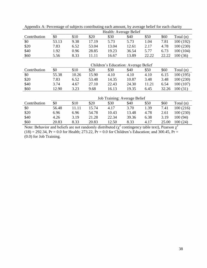
Appendix A: Percentage of subjects contributing each amount, by average belief for each charity
Health: Average Belief
Contribution $0 $10 $20 $30 $40 $50 $60 Total (n)
$0 53.13 9.38 17.19 5.73 5.73 1.04 7.81 100 (192)
$20 7.83 6.52 53.04 13.04 12.61 2.17 4.78 100 (230)
$40 1.92 0.96 28.85 19.23 36.54 5.77 6.73 100 (104)
$60 5.56 8.33 11.11 16.67 13.89 22.22 22.22 100 (36)
Children’s Education: Average Belief
Contribution $0 $10 $20 $30 $40 $50 $60 Total (n)
$0 55.38 10.26 15.90 4.10 4.10 4.10 6.15 100 (195)
$20 7.83 6.52 53.48 14.35 10.87 3.48 3.48 100 (230)
$40 3.74 4.67 27.10 22.43 24.30 11.21 6.54 100 (107)
$60 12.90 3.23 9.68 16.13 19.35 6.45 32.26 100 (31)
Job Training: Average Belief
Contribution $0 $10 $20 $30 $40 $50 $60 Total (n)
$0 56.48 11.11 15.74 4.17 3.70 1.39 7.41 100 (216)
$20 6.96 6.96 54.78 10.43 13.48 4.78 2.61 100 (230)
$40 4.26 3.19 21.28 22.34 39.36 6.38 3.19 100 (94)
$60 20.83 8.33 20.83 12.50 8.33 4.17 25.00 100 (24)
Note: Behavior and beliefs are not randomly distributed (χ2 contingency table text), Pearson χ
2
(18) = 292.34, Pr = 0.0 for Health; 273.22, Pr = 0.0 for Children’s Education; and 300.45, Pr =
(0.0) for Job Training.
39
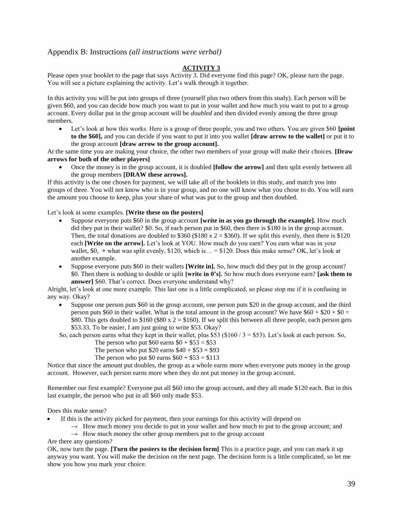
Appendix B: Instructions (all instructions were verbal)
ACTIVITY 3
Please open your booklet to the page that says Activity 3. Did everyone find this page? OK, please turn the page.
You will see a picture explaining the activity. Let’s walk through it together.
In this activity you will be put into groups of three (yourself plus two others from this study). Each person will be
given $60, and you can decide how much you want to put in your wallet and how much you want to put to a group
account. Every dollar put in the group account will be doubled and then divided evenly among the three group
members.
Let’s look at how this works. Here is a group of three people, you and two others. You are given $60 [point
to the $60], and you can decide if you want to put it into you wallet [draw arrow to the wallet] or put it to
the group account [draw arrow to the group account].
At the same time you are making your choice, the other two members of your group will make their choices. [Draw
arrows for both of the other players]
Once the money is in the group account, it is doubled [follow the arrow] and then split evenly between all
the group members [DRAW these arrows].
If this activity is the one chosen for payment, we will take all of the booklets in this study, and match you into
groups of three. You will not know who is in your group, and no one will know what you chose to do. You will earn
the amount you choose to keep, plus your share of what was put to the group and then doubled.
Let’s look at some examples. [Write these on the posters]
Suppose everyone puts $60 in the group account [write in as you go through the example]. How much
did they put in their wallet? $0. So, if each person put in $60, then there is $180 is in the group account.
Then, the total donations are doubled to $360 ($180 x 2 = $360). If we split this evenly, then there is $120
each [Write on the arrow]. Let’s look at YOU. How much do you earn? You earn what was in your
wallet, $0, + what was split evenly, $120, which is… = $120. Does this make sense? OK, let’s look at
another example.
Suppose everyone puts $60 in their wallets [Write in]. So, how much did they put in the group account?
$0. Then there is nothing to double or split [write in 0’s]. So how much does everyone earn? [ask them to
answer] $60. That’s correct. Does everyone understand why?
Alright, let’s look at one more example. This last one is a little complicated, so please stop me if it is confusing in
any way. Okay?
Suppose one person puts $60 in the group account, one person puts $20 in the group account, and the third
person puts $60 in their wallet. What is the total amount in the group account? We have $60 + $20 + $0 =
$80. This gets doubled to $160 ($80 x 2 = $160). If we split this between all three people, each person gets
$53.33. To be easier, I am just going to write $53. Okay?
So, each person earns what they kept in their wallet, plus $53 ($160 / 3 = $53). Let’s look at each person. So,
The person who put $60 earns $0 + $53 = $53
The person who put $20 earns $40 + $53 = $93
The person who put $0 earns $60 + $53 = $113
Notice that since the amount put doubles, the group as a whole earns more when everyone puts money in the group
account. However, each person earns more when they do not put money in the group account.
Remember our first example? Everyone put all $60 into the group account, and they all made $120 each. But in this
last example, the person who put in all $60 only made $53.
Does this make sense?
If this is the activity picked for payment, then your earnings for this activity will depend on
→ How much money you decide to put in your wallet and how much to put to the group account; and
→ How much money the other group members put to the group account
Are there any questions?
OK, now turn the page. [Turn the posters to the decision form] This is a practice page, and you can mark it up
anyway you want. You will make the decision on the next page. The decision form is a little complicated, so let me
show you how you mark your choice.
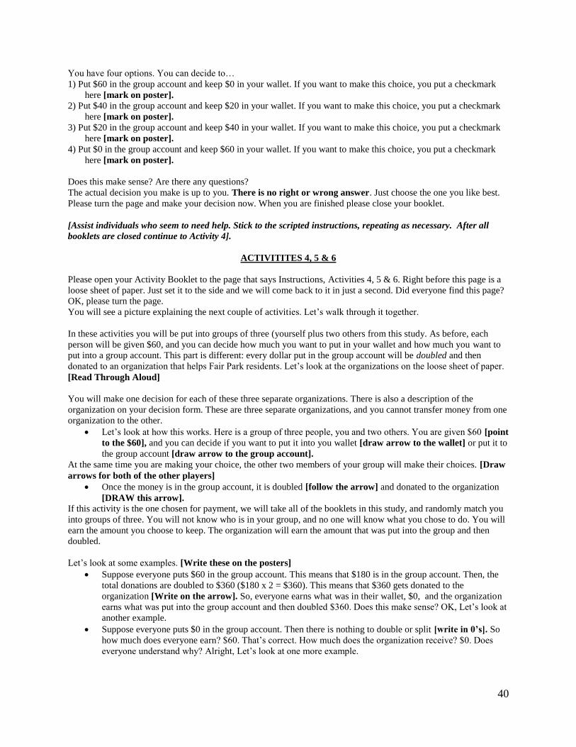
40
You have four options. You can decide to…
1) Put $60 in the group account and keep $0 in your wallet. If you want to make this choice, you put a checkmark
here [mark on poster].
2) Put $40 in the group account and keep $20 in your wallet. If you want to make this choice, you put a checkmark
here [mark on poster].
3) Put $20 in the group account and keep $40 in your wallet. If you want to make this choice, you put a checkmark
here [mark on poster].
4) Put $0 in the group account and keep $60 in your wallet. If you want to make this choice, you put a checkmark
here [mark on poster].
Does this make sense? Are there any questions?
The actual decision you make is up to you. There is no right or wrong answer. Just choose the one you like best.
Please turn the page and make your decision now. When you are finished please close your booklet.
[Assist individuals who seem to need help. Stick to the scripted instructions, repeating as necessary. After all
booklets are closed continue to Activity 4].
ACTIVITITES 4, 5 & 6
Please open your Activity Booklet to the page that says Instructions, Activities 4, 5 & 6. Right before this page is a
loose sheet of paper. Just set it to the side and we will come back to it in just a second. Did everyone find this page?
OK, please turn the page.
You will see a picture explaining the next couple of activities. Let’s walk through it together.
In these activities you will be put into groups of three (yourself plus two others from this study. As before, each
person will be given $60, and you can decide how much you want to put in your wallet and how much you want to
put into a group account. This part is different: every dollar put in the group account will be doubled and then
donated to an organization that helps Fair Park residents. Let’s look at the organizations on the loose sheet of paper.
[Read Through Aloud]
You will make one decision for each of these three separate organizations. There is also a description of the
organization on your decision form. These are three separate organizations, and you cannot transfer money from one
organization to the other.
Let’s look at how this works. Here is a group of three people, you and two others. You are given $60 [point
to the $60], and you can decide if you want to put it into you wallet [draw arrow to the wallet] or put it to
the group account [draw arrow to the group account].
At the same time you are making your choice, the other two members of your group will make their choices. [Draw
arrows for both of the other players]
Once the money is in the group account, it is doubled [follow the arrow] and donated to the organization
[DRAW this arrow]. If this activity is the one chosen for payment, we will take all of the booklets in this study, and randomly match you
into groups of three. You will not know who is in your group, and no one will know what you chose to do. You will
earn the amount you choose to keep. The organization will earn the amount that was put into the group and then
doubled.
Let’s look at some examples. [Write these on the posters]
Suppose everyone puts $60 in the group account. This means that $180 is in the group account. Then, the
total donations are doubled to $360 ($180 x 2 = $360). This means that $360 gets donated to the
organization [Write on the arrow]. So, everyone earns what was in their wallet, $0, and the organization
earns what was put into the group account and then doubled $360. Does this make sense? OK, Let’s look at
another example.
Suppose everyone puts $0 in the group account. Then there is nothing to double or split [write in 0’s]. So
how much does everyone earn? $60. That’s correct. How much does the organization receive? $0. Does
everyone understand why? Alright, Let’s look at one more example.

41
Suppose one person puts $60 in the group account, one person puts $20 in the group account, and the third
person puts $60 in their wallet. What is the total amount in the group account? We have $60 + $20 + $0 =
$80. This gets doubled to $160 ($80 x 2 = $160).
Each person earns what they kept in their wallet
The person who put $60 in the group account earns $0
The person who put $20 in the group account earns $40
The person who put $0 in the group account earns $60
The organization receives $160
Notice that since the amount put doubles, the organization earns more when everyone puts money in the group
account. However, each person earns more when they do not put money in the group account.
Remember our first example? Everyone put all $60 into the group account, and they all made $0 each, and the
organization made $360. But in this last example, the person who put in all $60 made $0 and the organization
received $160.
Does this make sense?
If this is the activity chosen for payment, then your earnings for this activity will be determined by
→ How much money you decide to put in your wallet and how much to put to the group account;
→ Money sent to the group account will be donated to an organization that provides one of the following
services for Fair Park residents: Healthcare, Childcare, or Job training.
→ The organization earns the amount donated to the group account, including the amount doubled.
If you want, you can wait until everyone is paid and watch us write the check for the organization. You can even go
with us to the mailbox if you like. Are there any questions?
OK, now turn the page. [Turn the posters to the decision form] Let me show you how you mark your choice.
As before, you have four options. You can decide to… [Ask them some]
1) Put $60 in the group account and keep $0 in your wallet. If you want to make this choice, you put a checkmark
here [mark on poster].
2) Put $40 in the group account and keep $20 in your wallet. If you want to make this choice, you put a checkmark
here [mark on poster].
3) Put $20 in the group account and keep $40 in your wallet. If you want to make this choice, you put a checkmark
here [mark on poster].
4) Put $0 in the group account and keep $60 in your wallet. If you want to make this choice, you put a checkmark
here [mark on poster].
Does this make sense? Are there any questions?
The actual decision you make is up to you. There is no right or wrong answer. Just choose the one you like best.
You will place a checkmark in the box next to your choice. Raise your hand if you have a question and one of our
monitors will come to help you.
Before you make your decisions, I need to read out loud the descriptions of the organizations. The 3 organizations
are the following: [Read the insert out loud – The insert has the names and short description of each organization]
Please turn the page to Activity 4. You can now make your decision for activities 4, 5 and 6.
When you are finished with activity 6, there are a couple of short questions about what you did in Activities 3 -6. If
you have any questions, please raise your hand and one of our monitors will come by to help you. When you are
done with everything, please close your booklet.
[Assist individuals who seem to need help. Stick to the scripted instructions, repeating as necessary. After all
booklets are closed continue to Belief Elicitation].