Ethiopian Wheat Yield and Yield Gap Estimation:

A Small Area Integrated Data Approach

25 March 2015

Michael Mann James Warner

International Food Policy Research Institute (IFPRI) Addis Ababa, Ethiopia

INTERNATIONAL FOOD POLICY RESEARCH INSTITUTE

The International Food Policy Research Institute (IFPRI) was established in 1975. IFPRI is one of 15 agricultural research centers that receives principal funding from governments, private foundations, and international and regional organizations, most of which are members of the Consultative Group on International Agricultural Research (CGIAR).

RESEARCH FOR ETHIOPIA’S AGRICULTURE POLICY (REAP): ANALYTICAL SUPPORT FOR THE AGRICULTURAL TRANSFORMATION AGENCY (ATA)

IFPRI gratefully acknowledges the generous financial support from the Bill and Melinda Gates Foundation (BMGF) for REAP, a five-year project led by the International Food Policy Research Institute (IFPRI). REAP provides policy research support to the Ethiopian Agricultural Transformation Agency (ATA) to identify issues, design programs, track progress, and document best practices as a global public good. The ATA is an innovative quasi-governmental agency with the mandate to test and evaluate various technological and institutional interventions to raise agricultural productivity, enhance market efficiency, and improve food security in Ethiopia.

DISCLAIMER

This report has been prepared as an output for REAP and has not been reviewed by IFPRI’s Publication Review Committee. Any views expressed herein are those of the authors and do not necessarily reflect the policies or views of IFPRI.

AUTHORS

Michael Mann, George Washington University Assistant Professor, Geography Department mmann1123@email.gwu.edu James Warner, International Food Policy Research Institute Research Coordinator, Markets, Trade, and Institutions Division, Addis Ababa j.warner@cgiar.org

i

Table of Contents Abstract ........................................................................................................................................................ iv

1 Introduction .......................................................................................................................................... 5

1.1 Project Description ........................................................................................................................ 5

1.2 Combining Remote Sensing with Survey Data—Data Integration ............................................... 6

2 Methods ................................................................................................................................................ 8

2.1 Objectives and overview ............................................................................................................... 8

2.2 Data ............................................................................................................................................... 9

2.2.1 Survey Variables: ................................................................................................................... 9

2.2.2 Climate/Weather Variables: ............................................................................................... 10

2.2.3 Spatial Variables: ................................................................................................................. 11

2.2.4 Remotely Sensed Data: ....................................................................................................... 12

2.3 Econometric Methods ................................................................................................................. 15

2.3.1 Wheat Yield Model Estimation: .......................................................................................... 15

2.3.2 Model Tests: ........................................................................................................................ 16

2.3.3 Out-Of-Sample Performance: ............................................................................................. 17

2.3.4 Yield Gap Estimation Introduction: ..................................................................................... 17

2.3.5 Yield Gap Methodology: ..................................................................................................... 18

2.4 Results ......................................................................................................................................... 19

2.4.1 Wheat Output per Hectare: ................................................................................................ 19

2.4.2 Yield Gap Analysis: .............................................................................................................. 28

2.5 Discussion .................................................................................................................................... 31

2.5.1 Panel Wheat Output per Hectare Results ........................................................................... 31

2.5.2 Yield Gap Results ................................................................................................................. 33

2.5.3 Model Improvements ......................................................................................................... 34

2.5.4 Future Applications ............................................................................................................. 35

3 References .......................................................................................................................................... 37

3.1 Appendix A .................................................................................................................................. 40

3.2 Appendix B .................................................................................................................................. 43

ii

Table of Figures

Figure 1: Calculation of Climatic Water Deficit by Month .......................................................................... 10 Figure 2: EVI Time series examples by land cover class .............................................................................. 13 Figure 3: Example relating EVI time series to wheat yields ........................................................................ 14 Figure 4: Yield Gap Methodology ............................................................................................................... 17 Figure 5 Wheat output per hectare in quintals by woreda ........................................................................ 20 Figure 6: Effect of a hectare of chemical fertilizer application on wheat yield .......................................... 21 Figure 7: Effect of % of land planted as wheat on yields ............................................................................ 22 Figure 8: Effect of maximum EVI value on wheat yield .............................................................................. 23 Figure 9: Effect of area under the declining portion of the EVI curve on wheat yield ............................... 23 Figure 10: Effect of elevation on wheat yield ............................................................................................. 24 Figure 11: Effect of terrain slope on wheat yield ........................................................................................ 24 Figure 12: The effects of climatic water deficit on wheat yields ................................................................ 25 Figure 13: The effects of distance to Addis Ababa on wheat yields ........................................................... 25 Figure 14: The effects of population density on wheat yields .................................................................... 26 Figure 15: Spatial distribution of yield gaps as determined by climate clusters ........................................ 29 Figure 16 Distribution of yield gaps as determined by climate clusters ..................................................... 30

iii

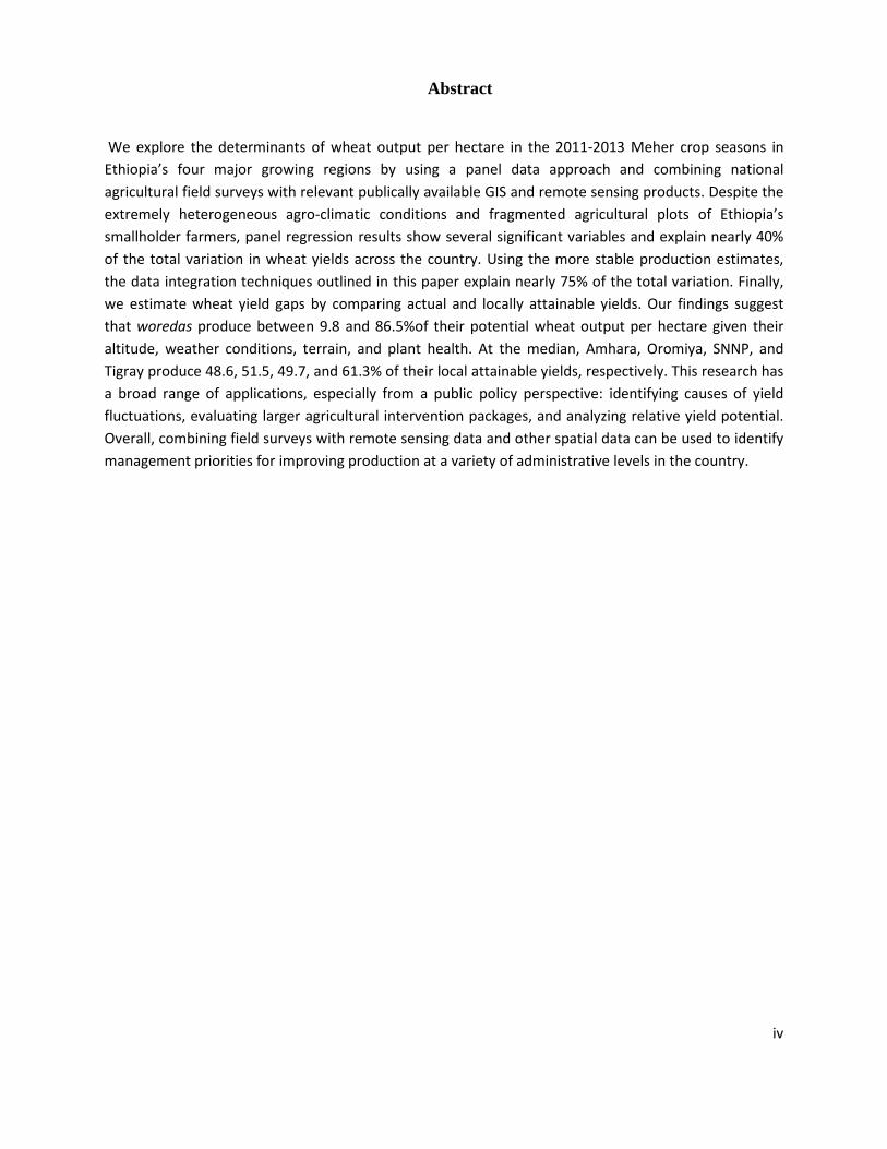
Abstract

We explore the determinants of wheat output per hectare in the 2011-2013 Meher crop seasons in Ethiopia’s four major growing regions by using a panel data approach and combining national agricultural field surveys with relevant publically available GIS and remote sensing products. Despite the extremely heterogeneous agro-climatic conditions and fragmented agricultural plots of Ethiopia’s smallholder farmers, panel regression results show several significant variables and explain nearly 40% of the total variation in wheat yields across the country. Using the more stable production estimates, the data integration techniques outlined in this paper explain nearly 75% of the total variation. Finally, we estimate wheat yield gaps by comparing actual and locally attainable yields. Our findings suggest that woredas produce between 9.8 and 86.5%of their potential wheat output per hectare given their altitude, weather conditions, terrain, and plant health. At the median, Amhara, Oromiya, SNNP, and Tigray produce 48.6, 51.5, 49.7, and 61.3% of their local attainable yields, respectively. This research has a broad range of applications, especially from a public policy perspective: identifying causes of yield fluctuations, evaluating larger agricultural intervention packages, and analyzing relative yield potential. Overall, combining field surveys with remote sensing data and other spatial data can be used to identify management priorities for improving production at a variety of administrative levels in the country.

iv

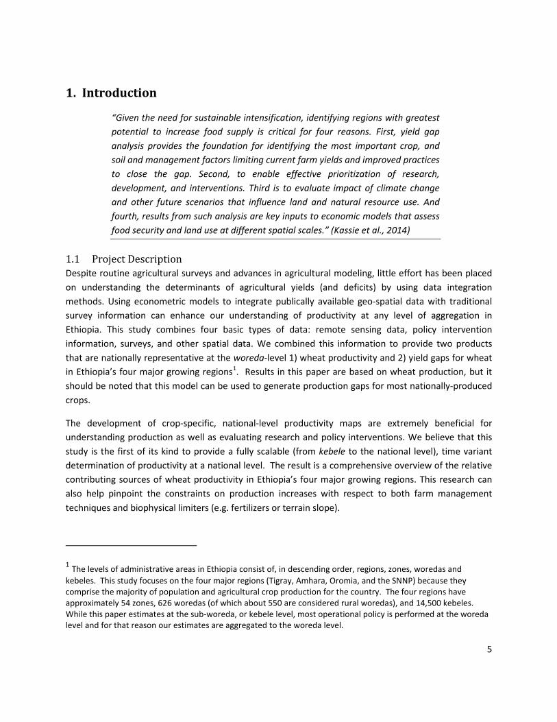
1. Introduction

“Given the need for sustainable intensification, identifying regions with greatest potential to increase food supply is critical for four reasons. First, yield gap analysis provides the foundation for identifying the most important crop, and soil and management factors limiting current farm yields and improved practices to close the gap. Second, to enable effective prioritization of research, development, and interventions. Third is to evaluate impact of climate change and other future scenarios that influence land and natural resource use. And fourth, results from such analysis are key inputs to economic models that assess food security and land use at different spatial scales.” (Kassie et al., 2014)

1.1 Project Description Despite routine agricultural surveys and advances in agricultural modeling, little effort has been placed on understanding the determinants of agricultural yields (and deficits) by using data integration methods. Using econometric models to integrate publically available geo-spatial data with traditional survey information can enhance our understanding of productivity at any level of aggregation in Ethiopia. This study combines four basic types of data: remote sensing data, policy intervention information, surveys, and other spatial data. We combined this information to provide two products that are nationally representative at the woreda-level 1) wheat productivity and 2) yield gaps for wheat in Ethiopia’s four major growing regions1. Results in this paper are based on wheat production, but it should be noted that this model can be used to generate production gaps for most nationally-produced crops.

The development of crop-specific, national-level productivity maps are extremely beneficial for understanding production as well as evaluating research and policy interventions. We believe that this study is the first of its kind to provide a fully scalable (from kebele to the national level), time variant determination of productivity at a national level. The result is a comprehensive overview of the relative contributing sources of wheat productivity in Ethiopia’s four major growing regions. This research can also help pinpoint the constraints on production increases with respect to both farm management techniques and biophysical limiters (e.g. fertilizers or terrain slope).

1 The levels of administrative areas in Ethiopia consist of, in descending order, regions, zones, woredas and kebeles. This study focuses on the four major regions (Tigray, Amhara, Oromia, and the SNNP) because they comprise the majority of population and agricultural crop production for the country. The four regions have approximately 54 zones, 626 woredas (of which about 550 are considered rural woredas), and 14,500 kebeles. While this paper estimates at the sub-woreda, or kebele level, most operational policy is performed at the woreda level and for that reason our estimates are aggregated to the woreda level.

5

There has been significant local interest in the creation of a production ‘gap map’ at the national level that displays actual yields versus potential yields. In this report, we present estimates of wheat yield gaps. These estimates are critical to understand the production potential of the agricultural sector as well as to provide information to guide interventions, both locally and nationally. Creating a production-gap map for Ethiopia is challenging for two reasons: there are extreme variations in agro-climatic conditions and the small size of farmers’ plots. Significant improvements in satellite technology and computing power in recent years, however, have made data processing and analysis for smallholder agriculture much more attainable and realistic. While not covered in this paper, future models could be developed to demonstrate the impact of climate change on production and the effectiveness of scaled-up policy interventions (e.g. blended fertilizers).

Traditional data analysis can be enhanced by using non-traditional data sources and more sophisticated algorithms along with a willingness to undertake interdisciplinary research. For example, freely accessible remote sensing data can provide real-time and retrospective information about plant characteristics, including plant health or water availability. Additionally, crowd-sourced data, like road maps on Open Street Map, can provide the first comprehensive look at Ethiopia’s complex and ever evolving transportation network. When combined with representative survey data, these non-traditional data sources can provide insight into the underlying human and natural systems that determine agricultural productivity and opens up new fields of inquiry. While this form of analysis has been developed in more economically developed nations with larger agricultural crop planting areas and more homogenous agro-ecological climates (Fontana 2005, Randall 2011), there has been relatively little work focusing on the smallholder African farmer.

1.2 Combining Remote Sensing with Survey Data—Data Integration

“Remote sensing thus offers a chance to increase the quantity and quality of survey data needed to identify on-farm yield constraints” (Nin-Pratt et al., 2011)

One of the principal objectives of this paper is to generate a unique integration of data previously unused in econometric analysis of smallholder agriculture. We believe that this general methodology has potentially far-reaching implications for research and analysis. The model in this paper relies on remote sensed data, survey data as well as other quantitative data. In addition, it is flexible enough to incorporate a wide variety of additional information. The goal is to enhance our understanding of the complex sources of agricultural productivity across Ethiopia’s diverse agro-ecological landscape. Further, advancements in this methodology, within the context of interdisciplinary work between soil scientists, economists, geographers and others, would provide additional refinements to this analysis.

Current academic and applied work in remote sensing is generally assessed at the pixel level, either at the macro (ie. Global, regional, state) or local scale (individual field) (Ferenz et al., 2004; Liu et al., 2005; Moran, Inoue, & Barnes, 1997; Prasad, Chai, Singh, & Kafatos, 2006; Serrano, Filella, & Peñuelas, 2000). Global studies rely on broad remote sensing tools, and the generalizations are, understandably, across multiple countries and agro-ecological zones (e.g. Licker et al., 2011). Field-level studies rely on localized

6

agricultural plots (of larger multi-hectare fields) and are combined with spatially consistent satellite imagery that creates relatively accurate yield estimates (Ferenz et al., 2004; Serrano et al., 2000). Typically, these farm-level research projects have taken place in more developed nations where agricultural plots are significantly larger (Moran et al., 1997; Swinton & Lowenberg-Deboer, 2001). To our knowledge, the type of national level analysis presented here, particularly for African smallholder farmers, has not been performed to date. In addition, most research of this kind has relied on crop models that use a relatively limited number of variables and are developed from an agro-ecological perspective. Here, the use of econometrics integrated with household surveys allows for increased flexibility and a better understanding of what influences Ethiopian farmers’ yields—estimates recorded by household and nationally representative surveys. In particular, we believe that we can better discern the influences of agro-climatic and economic factors for determining wheat productivity (Nin-Pratt et al., 2011). In this way, we hope to provide both researchers and policymakers with improved information to enhance analysis and interventions for the country.

Most developing nations engage in large annual crop surveys to provide an assessment of the current state of the agricultural sector, monitor progress of various interventions, as well as provide data for more detailed analysis by researchers. Ethiopia is an exceptional example of this and the Central Statistics Authority (CSA) engages in a massive annual survey, the Agricultural Sample Survey (AgSS), of over 45,000 rural households, which includes basic demographics, land size, input usage, as well as crop choice and output marketing. Rather than rely on the more common “farmer recollection” methodology, the survey includes crop cuts from sample fields. As far as we know, this crop cut methodology is unique to Sub-Saharan Africa. The AgSS is approximately ten times larger (in terms of sample households) than any other administered agricultural survey in the nation. For purposes here, a relatively large data set provides the most methodologically consistent and extensive coverage of the country available.

It is important to note that even though AgSS is the largest survey data in Ethiopia, remotely sensed and GIS data can be scaled to almost any level. As a result, the AgSS survey serves as the limiting data constraint in our analysis. Put another way, while the AgSS interviews approximately 45,000 households on an annual basis, the remote sensed data (e.g. enhanced vegetation index) includes about 44 million observations every 16 days (or about 1 billion data points annually). While there may be a temptation to rely on remote sensing data as the prominent method for evaluating production in agriculture, we believe, for reasons identified below, that the combination of survey and remote sensed data provides a superior analysis for productivity estimation.

Remote sensing can cover all areas of interest at a fairly detailed level. In this way, it can be combined with almost any survey, at any level of interest. Within the context of field-level analysis, remote sensing has at least three principal benefits. These benefits include bypassing or augmenting ground collected field measurements, allowing for yield estimates “at a range of spatial scales,” and reducing sampling error, which is usually associated with traditional surveys (Lobell, Ortiz-Monasterio, G., Naylor, & Falcon, 2005). The benefits of remote sensing, however, can be oversold, and care should be used to understand the methodology of using remote sensing information for data analysis purposes (Moran et al., 1997).

7

We do not see this as an either-or proposition, but rather, a synergy of data that enhances traditional research methods. While there are benefits and drawbacks to both, combining them can be superior to many types of data analysis. For example, conventional agricultural surveys have some subjectivity in responses and implementation can be expensive and relatively time-consuming; meanwhile remote sensing can provide an objective, standardized, and possibly cheaper information in a more timely fashion to aid growth, monitoring, and yield predictions (Ahmad et al., 2014; Lobell et al., 2005). On the other hand, surveys provide detailed information on farm labor, input choice, extension access, and other key determinants of productivity. Remote sensing is subject to aggregation issues (especially in areas of small farmer plots with extensive multi-cropping), cloud cover (especially during the rainy season), methodological choices by the researcher (eg. estimated planting time) as well as other drawbacks. Both methods have weaknesses and strengths, but by combing both, we can exploit a broader and more flexible set of data to model the determinants of wheat productivity.

There are a variety of data that can be combined with traditional survey studies to enhance our understanding of production and productivity in the agriculture sector. Because this relatively new field has few routinized methodologies (Ferenz et al., 2004), we welcome suggestions or critiques concerning our specific methods. This paper asserts that currently available remote sensing products cannot be exclusively used for most African smallholder agriculture modeling. However, if combined with other data, remote sensing provides additional information that is critical for estimating yields and yield gaps.

2. Methods

2.1 Objectives and overview The paper has two objectives, 1) to better understand the determinants of wheat yields for all wheat producing regions, and 2) to estimate yield gaps—the difference between a farmer’s actual yields and potential yields, given weather and edaphic conditions. We divide the potential determinant of wheat productivity into the following categories: agroecological, weather, farm management, policy and administration, infrastructure, and population. The econometric model described below uses a variety of data including satellite information, geo-spatial (distance to Addis Ababa, road density), elevation, hydrological data, terrain characteristics, agro-climatic data, administrative boundaries, population density (using census data divided by estimated hectares per kebele) as well as household survey variables from Ethiopia’s AGSS. Variables from the AgSS include chemical fertilizer, self-reported damage estimates, as well as the percentage of land dedicated to wheat. Spline functions are used to capture non-linear responses better. Because AgSS collects data for the same enumeration area (EA) for three years2, a lagged yield for that EA is also used. A dummy variable was also used to determine the effects of the Agricultural Growth Program (AGP) on identified relevant kebeles. While the EA is a sub-set of a kebele, we assume that the EA is representative of the kebele and make projections at the

2 An enumeration area (EA) is a sample area at the sub-kebele level. It is important to note that these EAs do not cross kebele boundaries and while they are a subset of the kebele we assume that they are representative of the kebele itself. This is a simplifying assumption that would benefit from additional analysis.

8

kebele level (other analysis, not included here, has been performed to demonstrate the relative homogeneity of the kebele-level administrative area). Much of the spatial data was collected at the 250 square meter resolution (6.25 hectares) and then summarized to the kebele administrative boundary.

2.2 Data “Geographic factors such as agroecological conditions, population distribution, and production and market locations and infrastructure are much more important in agricultural development strategy than in the development of other sectors of the economy” (Nin-Pratt et al., 2011)

This paper draws on eleven data sources in four major categories, including remote sensed data, survey data, mapping data (with GIS), and identified policy intervention woredas. It is important to stress that no primary data was collected, and, therefore, this model was generated with relatively little cost. Supplementing this model with either primary data or additional secondary data would improve its accuracy. The use of several additional sources of information such as weather-related data from the National Meteorological Agency (NMA), localized agricultural information from the respective Regional Bureaus of Agriculture, and additional remote sensing products, including higher resolution, might be used. Of particular importance is that whatever data is used, synergies are created when more traditional data is combined with satellite information.

2.2.1 Survey Variables: Primary data is obtained from the AGSS (2013). Survey data includes productivity and farm management variables covering three years of agricultural data (2011/2012 – 2013/2014 Meher crop seasons). The CSA takes a random sample of enumeration areas (EAs) that exist at the sub-kebele level, which are then weighted to estimate zones in their respective regions. Kebele population sampling weights were derived using the 2007 Ethiopian population census data (Population Census Commission, 2008) and adjusted over time using the World Bank’s annual agricultural population growth rates for Ethiopia (The World Bank, 2013). It is also important to emphasize that approximately 97% of the same EAs are sampled for a three-year period (this allows for a kebele panel data set to be used). For purposes here, we reconfigured the estimated areas to the individual kebele level, which means using the 20 households interviewed per EA and projecting this sample to cover the entire kebele. Field productivity is measured as the mean output per hectare (wheatOPH) in quintals per hectare and is an aggregated sample of between three and five crop cuts at the EA level. Areas with less than three samples per EA were dropped from the analysis to enhance stability of the estimates. Population density is measured as the total population per hectare (Popden). Other statistics on wheat production include the total hectares of chemical fertilizer application in a kebele (Wheatchemfert); total hectares of wheat irrigation (Irrigation); total hectares of wheat damaged by weather, pests or other external events (Damage); and the percentage of total area planted with wheat (LandWheat)3.

3 Total hectares planted might be considered an endogenous variable and evidence from the production model suggests that last year’s productivity has a positive impact on area planted. However, there are a variety of other

9

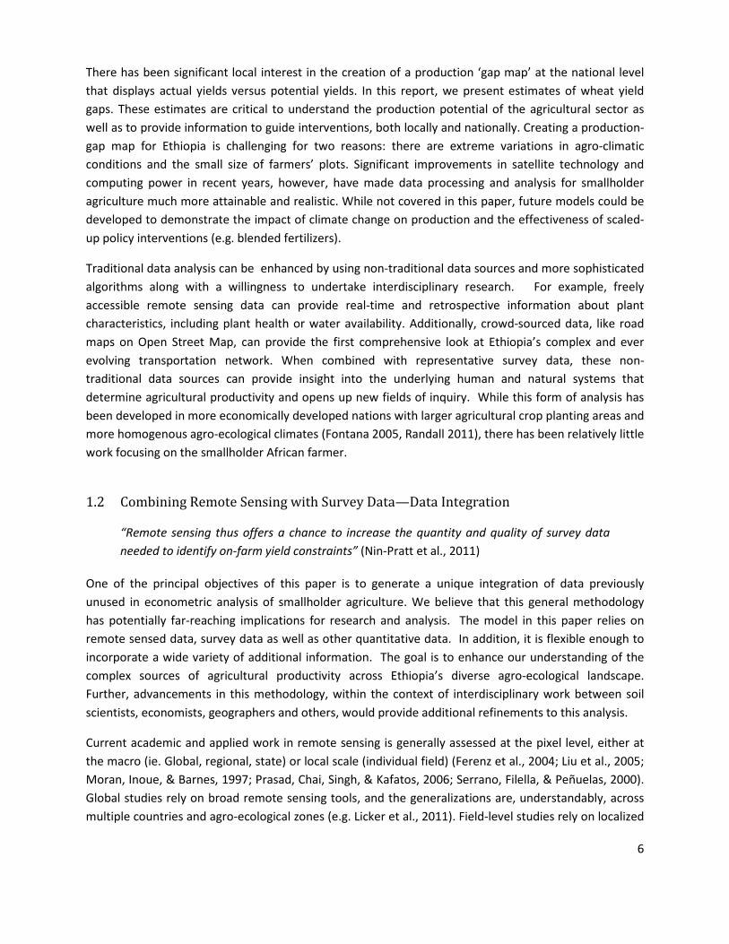
2.2.2 Climate/Weather Variables: Climatic Water Deficit (CWD) is retrieved at 0.5-degree resolution (a pixel 0.5 decimal degrees or approximately 50 kilometers on a side) and is an indicator of water available to plants (Willmott & Matsuura, 2001). CWD data is accessed via the University of Delaware’s web-based, Water-Budget, Interactive Modeling Program. Delaware’s monthly water budgets were estimated from a gridded monthly average temperature and total precipitation fields according to the Willmott et al. (C. J. Willmott, Rowe, & Mintz, 1985) version of the Thornthwaite water-budget procedure. Climatic water deficit (CWD) is the difference between actual evapotranspiration (AET) 4 and potential evapotranspiration (PET)5 (Major, 1967). A visual representation as seen in Figure 1, demonstrates that the amount of water moved through the ecosystem (AET-actual evapotranspiration) is determined by water supply (SUPPLY, through precipitation) and water demanded (PET-potential evapotranspiration, through evaporation from soils and plants). PET is determined not by the water supply but by the evaporative demand based on temperatures and plant and soil characteristics, if water is not a limiting factor. The climate deficit is the difference between the amount of water that could be moved through the system, if water was not limited, and the amount moved (Deficit).

Figure 1: Calculation of Climatic Water Deficit by Month

independent variables that control for traditionally productive areas and given the relative variability of output per hectare (weather, etc.), we believe that current productivity has a limited direct impact on actual area planted.

1. 4 The process by which water is transferred from the land to the atmosphere by evaporation from the soil and other surfaces and by transpiration from plants. 5PET is the level evapotranspiration by plants when water is a not limiting factor.

10

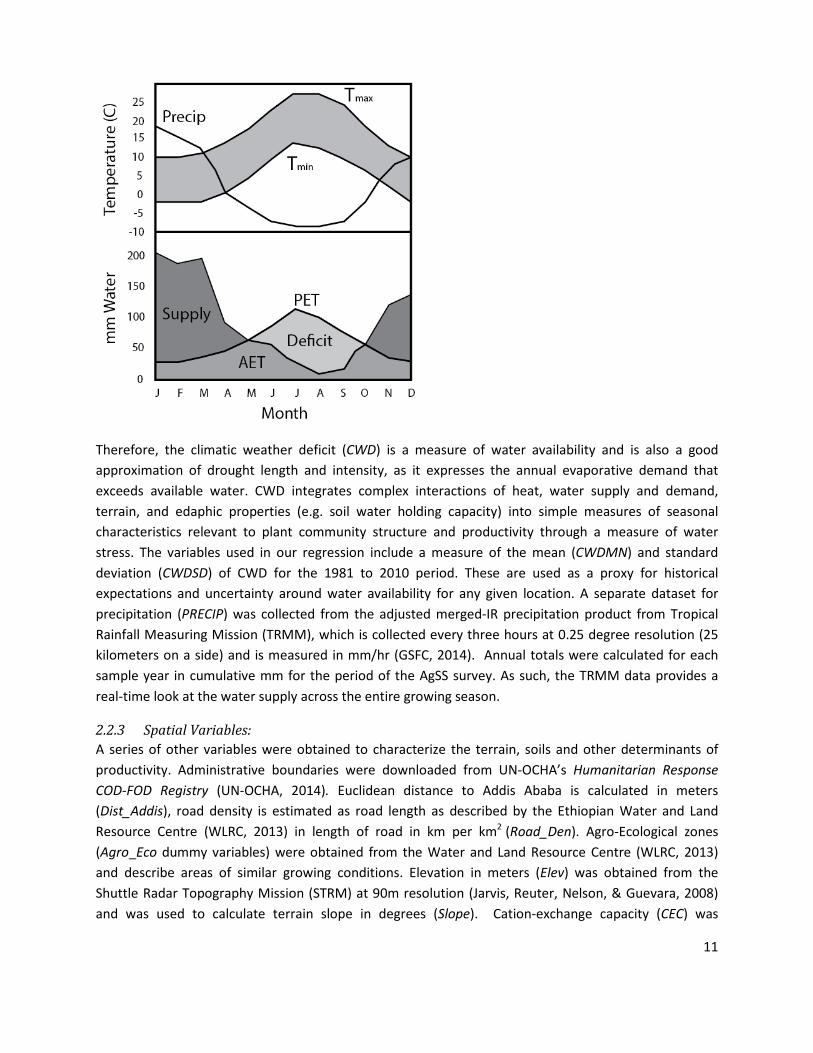
Therefore, the climatic weather deficit (CWD) is a measure of water availability and is also a good approximation of drought length and intensity, as it expresses the annual evaporative demand that exceeds available water. CWD integrates complex interactions of heat, water supply and demand, terrain, and edaphic properties (e.g. soil water holding capacity) into simple measures of seasonal characteristics relevant to plant community structure and productivity through a measure of water stress. The variables used in our regression include a measure of the mean (CWDMN) and standard deviation (CWDSD) of CWD for the 1981 to 2010 period. These are used as a proxy for historical expectations and uncertainty around water availability for any given location. A separate dataset for precipitation (PRECIP) was collected from the adjusted merged-IR precipitation product from Tropical Rainfall Measuring Mission (TRMM), which is collected every three hours at 0.25 degree resolution (25 kilometers on a side) and is measured in mm/hr (GSFC, 2014). Annual totals were calculated for each sample year in cumulative mm for the period of the AgSS survey. As such, the TRMM data provides a real-time look at the water supply across the entire growing season.

2.2.3 Spatial Variables: A series of other variables were obtained to characterize the terrain, soils and other determinants of productivity. Administrative boundaries were downloaded from UN-OCHA’s Humanitarian Response COD-FOD Registry (UN-OCHA, 2014). Euclidean distance to Addis Ababa is calculated in meters (Dist_Addis), road density is estimated as road length as described by the Ethiopian Water and Land Resource Centre (WLRC, 2013) in length of road in km per km2 (Road_Den). Agro-Ecological zones (Agro_Eco dummy variables) were obtained from the Water and Land Resource Centre (WLRC, 2013) and describe areas of similar growing conditions. Elevation in meters (Elev) was obtained from the Shuttle Radar Topography Mission (STRM) at 90m resolution (Jarvis, Reuter, Nelson, & Guevara, 2008) and was used to calculate terrain slope in degrees (Slope). Cation-exchange capacity (CEC) was

11

measured as the maximum quantity of total cations measured in meq+/100g dry soil, that a soil is capable of holding, at a given pH value, available for exchange with the soil solution. CEC was used as a measure of fertility and nutrient retention capacity (Leenaars, 2013). This data was accessed via the Africa Soils Profiles Database v 1.1. Other edaphic properties were also downloaded from the Africa Soils Database but were dropped from the final model due to statistical insignificance. The Agricultural Growth Program (AGP) interventions indicate whether or not the AgSS surveyed-areas operated under the AGP program during the sample period. The AGP intervention is a large-scale (83 initial woredas) project, funded by the World Bank, designed to increase productivity and marketization within high-potential areas. Intervention woredas were obtained from the ESSP II’s baseline report (IFPRI, 2013).

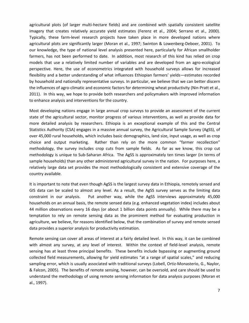
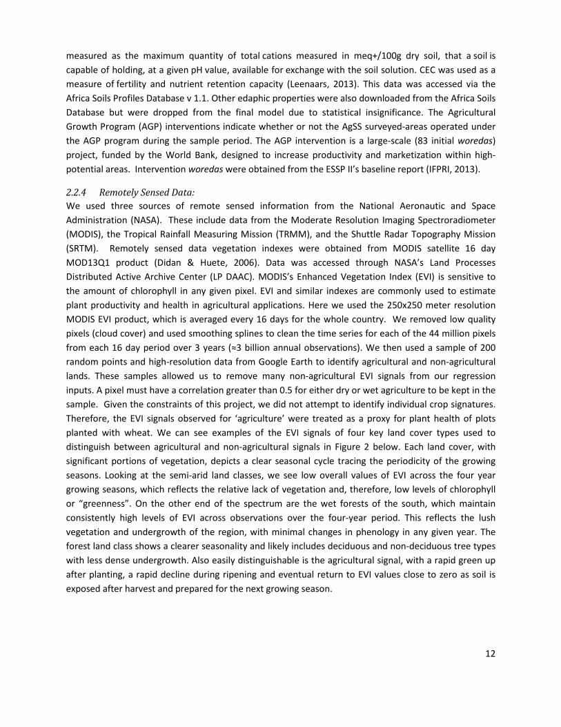
2.2.4 Remotely Sensed Data: We used three sources of remote sensed information from the National Aeronautic and Space Administration (NASA). These include data from the Moderate Resolution Imaging Spectroradiometer (MODIS), the Tropical Rainfall Measuring Mission (TRMM), and the Shuttle Radar Topography Mission (SRTM). Remotely sensed data vegetation indexes were obtained from MODIS satellite 16 day MOD13Q1 product (Didan & Huete, 2006). Data was accessed through NASA’s Land Processes Distributed Active Archive Center (LP DAAC). MODIS’s Enhanced Vegetation Index (EVI) is sensitive to the amount of chlorophyll in any given pixel. EVI and similar indexes are commonly used to estimate plant productivity and health in agricultural applications. Here we used the 250x250 meter resolution MODIS EVI product, which is averaged every 16 days for the whole country. We removed low quality pixels (cloud cover) and used smoothing splines to clean the time series for each of the 44 million pixels from each 16 day period over 3 years (≈3 billion annual observations). We then used a sample of 200 random points and high-resolution data from Google Earth to identify agricultural and non-agricultural lands. These samples allowed us to remove many non-agricultural EVI signals from our regression inputs. A pixel must have a correlation greater than 0.5 for either dry or wet agriculture to be kept in the sample. Given the constraints of this project, we did not attempt to identify individual crop signatures. Therefore, the EVI signals observed for ‘agriculture’ were treated as a proxy for plant health of plots planted with wheat. We can see examples of the EVI signals of four key land cover types used to distinguish between agricultural and non-agricultural signals in Figure 2 below. Each land cover, with significant portions of vegetation, depicts a clear seasonal cycle tracing the periodicity of the growing seasons. Looking at the semi-arid land classes, we see low overall values of EVI across the four year growing seasons, which reflects the relative lack of vegetation and, therefore, low levels of chlorophyll or “greenness”. On the other end of the spectrum are the wet forests of the south, which maintain consistently high levels of EVI across observations over the four-year period. This reflects the lush vegetation and undergrowth of the region, with minimal changes in phenology in any given year. The forest land class shows a clearer seasonality and likely includes deciduous and non-deciduous tree types with less dense undergrowth. Also easily distinguishable is the agricultural signal, with a rapid green up after planting, a rapid decline during ripening and eventual return to EVI values close to zero as soil is exposed after harvest and prepared for the next growing season.

12

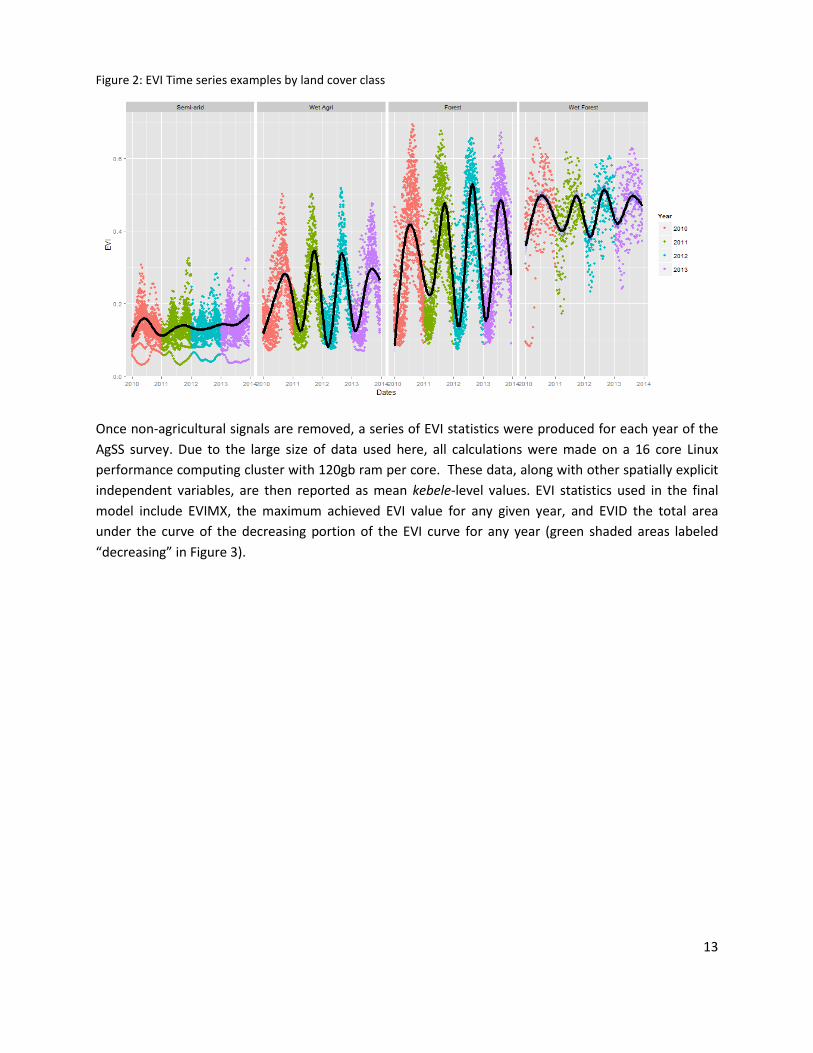
Figure 2: EVI Time series examples by land cover class

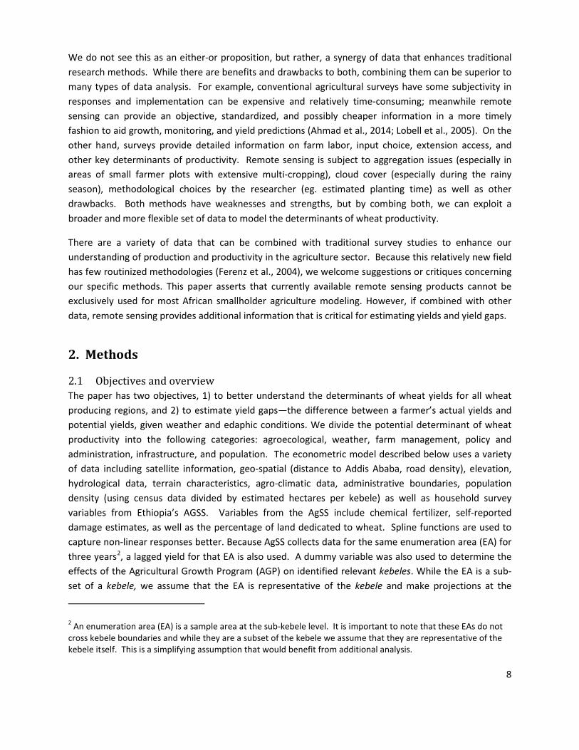
Once non-agricultural signals are removed, a series of EVI statistics were produced for each year of the AgSS survey. Due to the large size of data used here, all calculations were made on a 16 core Linux performance computing cluster with 120gb ram per core. These data, along with other spatially explicit independent variables, are then reported as mean kebele-level values. EVI statistics used in the final model include EVIMX, the maximum achieved EVI value for any given year, and EVID the total area under the curve of the decreasing portion of the EVI curve for any year (green shaded areas labeled “decreasing” in Figure 3).

13

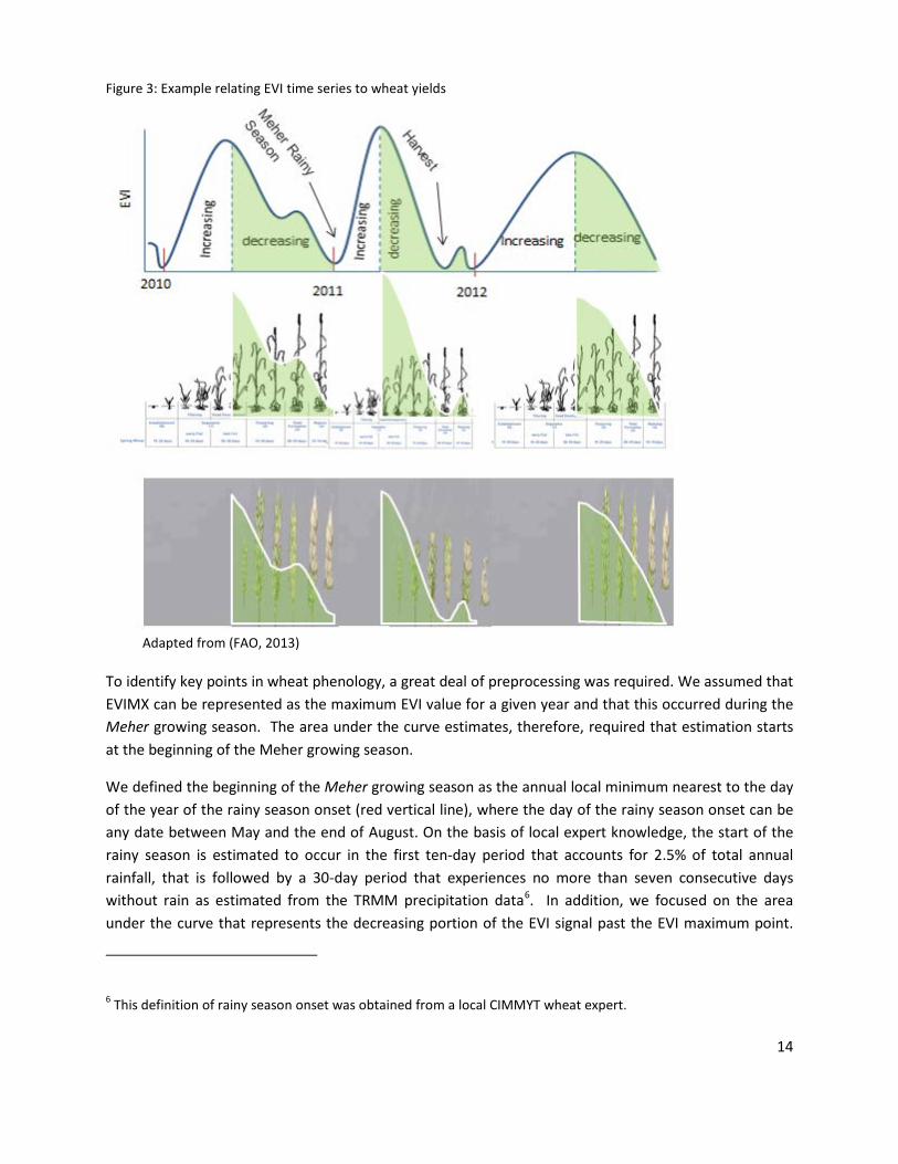
Figure 3: Example relating EVI time series to wheat yields

Adapted from (FAO, 2013) To identify key points in wheat phenology, a great deal of preprocessing was required. We assumed that EVIMX can be represented as the maximum EVI value for a given year and that this occurred during the Meher growing season. The area under the curve estimates, therefore, required that estimation starts at the beginning of the Meher growing season.

We defined the beginning of the Meher growing season as the annual local minimum nearest to the day of the year of the rainy season onset (red vertical line), where the day of the rainy season onset can be any date between May and the end of August. On the basis of local expert knowledge, the start of the rainy season is estimated to occur in the first ten-day period that accounts for 2.5% of total annual rainfall, that is followed by a 30-day period that experiences no more than seven consecutive days without rain as estimated from the TRMM precipitation data6. In addition, we focused on the area under the curve that represents the decreasing portion of the EVI signal past the EVI maximum point.

6 This definition of rainy season onset was obtained from a local CIMMYT wheat expert.

14

This period of the phenological cycle matches roughly with the head development and yield formation in the plant. Therefore, inadequate water availability during these periods have been shown to strongly affect yields (FAO, 2013). A stylized example is provided in Figure 3, where the top panel traces the ‘greenup’ of plants after planting until the reach some peak ‘greeness’ as maximal levels of chlorophyll and leaf area are reached. Greenness then declines as the heading periods gives way to ripening. Future refinements could include more careful calibration of the EVI index to the phenological growth of wheat or contrasting EVI signatures to other crops.

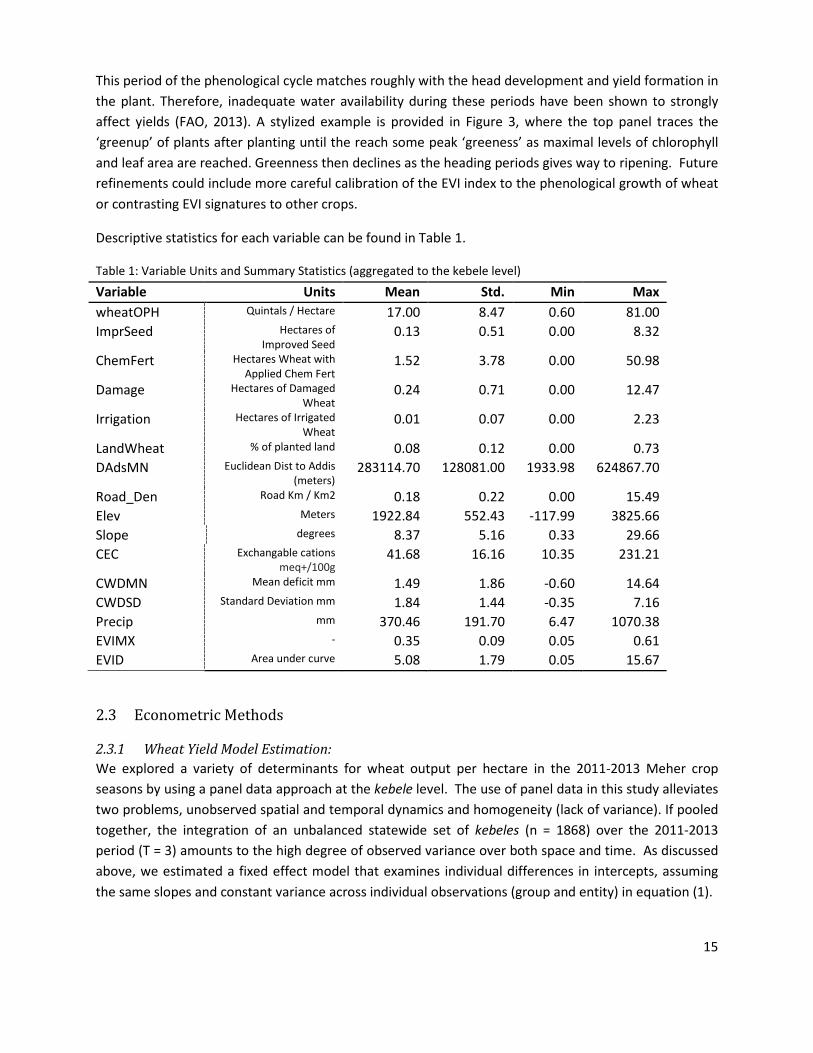
Descriptive statistics for each variable can be found in Table 1.

Table 1: Variable Units and Summary Statistics (aggregated to the kebele level)

Variable Units Mean Std. Min Max wheatOPH Quintals / Hectare 17.00 8.47 0.60 81.00 ImprSeed Hectares of

Improved Seed 0.13 0.51 0.00 8.32

ChemFert Hectares Wheat with Applied Chem Fert

1.52 3.78 0.00 50.98

Damage Hectares of Damaged Wheat

0.24 0.71 0.00 12.47

Irrigation Hectares of Irrigated Wheat

0.01 0.07 0.00 2.23

LandWheat % of planted land 0.08 0.12 0.00 0.73 DAdsMN Euclidean Dist to Addis

(meters) 283114.70 128081.00 1933.98 624867.70

Road_Den Road Km / Km2 0.18 0.22 0.00 15.49 Elev Meters 1922.84 552.43 -117.99 3825.66 Slope degrees 8.37 5.16 0.33 29.66 CEC Exchangable cations

meq+/100g 41.68 16.16 10.35 231.21

CWDMN Mean deficit mm 1.49 1.86 -0.60 14.64 CWDSD Standard Deviation mm 1.84 1.44 -0.35 7.16 Precip mm 370.46 191.70 6.47 1070.38 EVIMX - 0.35 0.09 0.05 0.61 EVID Area under curve 5.08 1.79 0.05 15.67

2.3 Econometric Methods

2.3.1 Wheat Yield Model Estimation: We explored a variety of determinants for wheat output per hectare in the 2011-2013 Meher crop seasons by using a panel data approach at the kebele level. The use of panel data in this study alleviates two problems, unobserved spatial and temporal dynamics and homogeneity (lack of variance). If pooled together, the integration of an unbalanced statewide set of kebeles (n = 1868) over the 2011-2013 period (T = 3) amounts to the high degree of observed variance over both space and time. As discussed above, we estimated a fixed effect model that examines individual differences in intercepts, assuming the same slopes and constant variance across individual observations (group and entity) in equation (1).

15

(1) 𝑦𝑦𝑖𝑖𝑖𝑖 = (𝛼𝛼 + 𝜇𝜇𝑤𝑤) + 𝛽𝛽𝛽𝛽𝑖𝑖𝑖𝑖 + δ𝑊𝑊𝑖𝑖𝑖𝑖 + ω𝑀𝑀𝑖𝑖𝑖𝑖 + φ𝑃𝑃𝑖𝑖𝑖𝑖 + γ𝐼𝐼𝑖𝑖𝑖𝑖 + ρ𝑃𝑃𝑖𝑖𝑖𝑖 + 𝜃𝜃𝑦𝑦𝑖𝑖 𝑖𝑖−1 + 𝑣𝑣𝑖𝑖𝑖𝑖 Where 𝑦𝑦𝑖𝑖𝑖𝑖 is wheat output per hectare for kebele i in time t. 𝛽𝛽𝛽𝛽𝑖𝑖𝑖𝑖 is a Kx1 vector of regression coefficients (𝛽𝛽 ) for descriptive variables 𝛽𝛽𝑖𝑖𝑖𝑖 , where K is the number of descriptive variables. 𝛽𝛽𝛽𝛽𝑖𝑖𝑖𝑖 includes relevant exogenous agroecological (Elev, Slope, CEC, AgEcoFactor) determinants of wheat productivity, δ𝑊𝑊𝑖𝑖𝑖𝑖includes weather and climate (Precip, Damage, CWDMN, CWDSD, EVIMX, EVID), ω𝑀𝑀𝑖𝑖𝑖𝑖 includes management variables (ImprSeed, ChemFert, Irrigation, LandWheat), φ𝑃𝑃𝑖𝑖𝑖𝑖 contains a policy and administration variable (AGP), γ𝐼𝐼𝑖𝑖𝑖𝑖 represents infrastructure variables (DAdsMN, Road_Den), and ρ𝑃𝑃𝑖𝑖𝑖𝑖 controls for effects of population (Popden). 𝜇𝜇𝑤𝑤 is a vector of zone-level fixed effects constants that controls for unobserved characteristics of each woreda w7. 𝜃𝜃𝑦𝑦𝑖𝑖 𝑖𝑖−1 is a vector of regression coefficients for temporally lagged values of y for period t – 1 (i.e. last Meher’s output per hectare in the same kebele), and 𝑣𝑣𝑖𝑖𝑖𝑖 is a N × T matrix of disturbances. Controlling for both time and zonal fixed effects allows us to disentangle the effect of temporal and spatial heterogeneity of omitted variables. To control for potential heteroskedasticity, we estimate eq (1) using Huber-White sandwich estimators (Huber, 1967; White, 1980). The statistical significance of each variable is tested and is reported in the text as a p-value with estimates with p < 0.05 being considered statistically significant, and p > 0.05 being insignificant.

Model Tests:

Pre-estimation: In order to choose between Pooled, Fixed Effects (FE), Random Effects (RE) models, we used an F-test, Breusch-Pagan LM test, and Hausman Test. We tested if individual specific variance components were zero (𝐻𝐻𝑜𝑜: 𝜎𝜎𝑢𝑢2 = 0) with the Breusch-Pagan Lagrange multiplier (BPLM) test adjusted for unbalanced panels (Sosa-Escudero & Bera, 2008). The adjusted BPLM test does not reject the null (p>0.09) and concluded that the RE model is not able to handle heterogeneity better than pooled OLS (ie inconsistent). We tested for Fixed Effects using an F-test (𝐻𝐻𝑜𝑜:𝜇𝜇1 = ⋯ = 𝜇𝜇𝑛𝑛−1 = 0), we then rejected the null hypothesis that all woreda-level dummy variables are zero (p<0.01) and concluded that there is a significant fixed effect. We reinforced the use of FE with the use of the Hausman test (Hausman, 1978), where we tested if the individual effects are uncorrelated with a regressor in the model. Here, we rejected the null (p<0.01) and concluded that individual effects 𝜇𝜇𝑖𝑖 are significantly correlated with at least one regressor. Therefore, the use of RE is problematic.

Post-estimation: We tested for global spatial autocorrelation in the error term with the use of an augmented Moran’s I Test for model residuals (Cliff & Ord, 1981). We could not reject the null of no spatial autocorrelation in the residual (p>0.36).

7 A recent research study of yields at the global-level acknowledged that crop yield patterns do follow administrative boundaries (Licker et al., 2011). This points to the relative importance of nationally directed crop management practices over just biophysical areas determining relative yields. Therefore, we incorporate zonal level administrative dummy variables to depict potential variations in administrative capacity in facilitating agricultural implementations and other varying institutional issues.

16

2.3.2 Out-Of-Sample Performance: The use of environmental along with topology and remotely sensed data enabled us to estimate wheat output per hectare out-of-sample (outside of the original AgSS survey). In order to predict kebeles outside of the AgSS survey, survey specific questions were dropped from (1) with predictions being made from the simplified regression (results in Table 2 - Out-of-Sample). These can be used to estimate yields or yield gaps on a kebele-by-kebele, year-by-year basis. We used a k-fold cross-validation on the final model to evaluate the model's ability to fit out-of-sample data (Lachenbruch & Mickey, 1968). This procedure splits the data randomly into k partitions. Then for each partition, it fits the specified model using the other k-1 groups and uses the resulting parameters to predict out-of-sample the dependent variable in the unused group. Accuracy metrics are then reported for each out-of-sample prediction in Appendix A, Table A1.

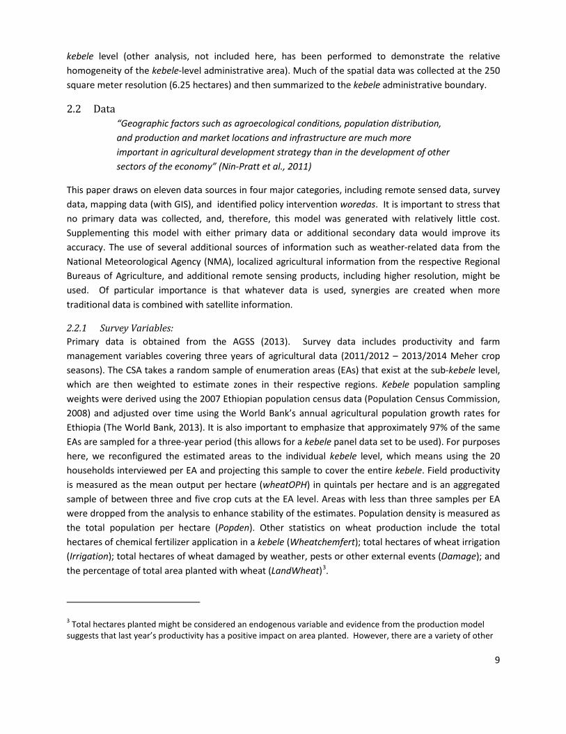
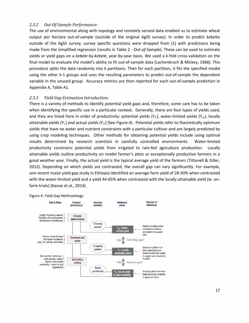
2.3.3 Yield Gap Estimation Introduction: There is a variety of methods to identify potential yield gaps and, therefore, some care has to be taken when identifying the specific use in a particular context. Generally, there are four types of yields used, and they are listed here in order of productivity: potential yields (YP), water-limited yields (Yw), locally attainable yields (YL) and actual yields (YA) (See Figure 4). Potential yields refer to theoretically optimum yields that have no water and nutrient constraints with a particular cultivar and are largely predicted by using crop modeling techniques. Other methods for obtaining potential yields include using optimal results determined by research scientists in carefully controlled environments. Water-limited productivity constrains potential yields from irrigated to rain-fed agriculture production. Locally attainable yields outline productivity on model farmer’s plots or exceptionally productive farmers in a good weather year. Finally, the actual yield is the typical average yield of the farmers (Tittonell & Giller, 2012). Depending on which yields are contrasted, the overall gap can vary significantly. For example, one recent maize yield gap study in Ethiopia identified an average farm yield of 28-30% when contrasted with the water-limited yield and a yield 44-65% when contrasted with the locally attainable yield (ie. on-farm trials) (Kassie et al., 2014).

Figure 4: Yield Gap Methodology

17

(Tittonell & Giller, 2012)

In this study, we used a variation of (YL-YA) comparing actual yields to locally attainable yields as defined by the productivity of the 90th percentile kebele within an agro-ecologically similar cluster. Broadly speaking, we wanted to compare aggregated locally attainable yields with actual yields from other comparable kebeles with similar growing conditions. We identified kebeles with similar growing conditions, as described in more detail in the next section, through a clustering algorithm that groups kebeles with similar elevation, climate norms, and water availability. These clusters are time-variant, so a kebele’s membership will change year to year with growing conditions. We believe these clusters provide relatively homogenous weather and agroecological conditions, which are required for realistic comparisons of actual and attainable yields (Nin-Pratt et al., 2011).

These gaps should be slightly less than what is typically presented as a yield gap for at least two reasons. First, YL is obtained from yields reported by farmers in the AgSS survey, and not the experimental farm or water-limited yields. Second, our methodology aggregates to the kebele level, thereby reducing high individual productive outliers. The result is a lower, but more generalizable production gap. One advantage of the methodology is that it can be generally assumed that the reference technologies are similar across all producers, so closing these gaps are reasonably attainable with appropriate interventions. Put another way, contrasting potential yields with actual yields would create an unattainable gap, given the current level of access to technology, at least in the near term. The estimated gaps provided here are most likely to be closed by providing greater access to improved agro-economic management practices (Nin-Pratt et al., 2011).

2.3.4 Yield Gap Methodology: We explored methods that characterized potential yields based on real-world observations in Ethiopia, rather than on expectations based on idealized or simulated conditions. Here we assumed that the 90th percentile is the locally attainable yield which can be contrasted with actual yields of the other comparable areas (YL-YA).

We identified eight kebele groupings, with similar agroecological characteristics using a multidimensional clustering algorithm. K-means clustering partitions multidimensional data into k clusters of similar data (k=8). Distance to the multidimensional cluster mean determines a kebele’s membership in any cluster. Clusters are iteratively determined with new memberships assigned to observations (i.e. kebeles) until no observations switch memberships. At this point, eq (2) will reach its minimum value. In other words, given a set of observations (x1, x2,.., xn) where each observation is a multidimensional vector (containing information about climate, weather etc.), the K-mean algorithm aims to partition the n observations into k sets S = {S1, S2,…, Sk} in order to minimize within the cluster variance (sum of squares) as described by:

(2) min𝑠𝑠 ∑ ∑ |𝑥𝑥 − 𝜌𝜌𝑖𝑖|2𝑥𝑥∈𝑆𝑆𝑖𝑖𝑘𝑘𝑖𝑖=1

Where 𝜌𝜌𝑖𝑖 is the mean value of observations in cluster Si. Here we partition the data based on four weather and agroecological categories and a total of five variables. These variables include: elevation (Elev), precipitation (Precip), greenness during the late season (EVID), mean climatic water deficit

18

(CWDMN), and standard deviation of climatic water deficit (CWDSD). These variables were chosen as key determinants from the estimation of equation (1) and can be considered representative of climate, weather, and topography. Equation (2) is estimated as a panel with cluster membership varying year to year given changes in time-variant conditions (precipitation, greenness). Yield performance of any kebele can then be compared to the distribution of yields from kebeles with similar climate, weather, and terrain on a year-to-year basis. Wheat yield gaps are calculated as follows:

(3) −100 �1 − 𝑌𝑌𝐴𝐴𝑌𝑌𝐿𝐿�

Where 𝑌𝑌𝐴𝐴 is actual yields as estimated out-of-sample from the panel regression estimated in eq (1), and 𝑌𝑌𝐿𝐿 is local attainable yields, defined as the 90th percentile of the distributions described by a kebele’s cluster membership described above. Due to interest that these gaps be reported at the woreda level, kebele level estimates are aggregated to the woreda level using an area weighted sum.

2.4 Results

2.4.1 Wheat Output per Hectare: The following section outlines the results of the panel regression by estimating wheat output per hectare8 . Regression estimates are reported in Table 2, and estimates of output hectare are presented in Figure 5 below. Given the large sample area and aggregation to the kebele, initial results are promising with all coefficients displaying the correct sign and statistical significance and an overall R-square of almost 0.40 for the model. Given stability of growing areas, the comparatively easier task of estimating total production at the kebele level, our model captured nearly 75% of variation (Table B1, Appendix B).

8 A more in-depth discussion concerning causes and implications is provided in Section 3.3.

19

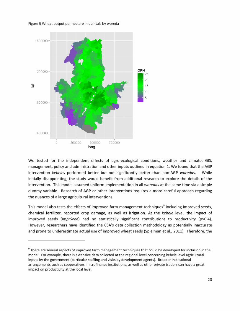
Figure 5 Wheat output per hectare in quintals by woreda

We tested for the independent effects of agro-ecological conditions, weather and climate, GIS, management, policy and administration and other inputs outlined in equation 1. We found that the AGP intervention kebeles performed better but not significantly better than non-AGP woredas. While initially disappointing, the study would benefit from additional research to explore the details of the intervention. This model assumed uniform implementation in all woredas at the same time via a simple dummy variable. Research of AGP or other interventions requires a more careful approach regarding the nuances of a large agricultural interventions.

This model also tests the effects of improved farm management techniques9 including improved seeds, chemical fertilizer, reported crop damage, as well as irrigation. At the kebele level, the impact of improved seeds (ImprSeed) had no statistically significant contributions to productivity (p>0.4). However, researchers have identified the CSA’s data collection methodology as potentially inaccurate and prone to underestimate actual use of improved wheat seeds (Spielman et al., 2011). Therefore, the

9 There are several aspects of improved farm management techniques that could be developed for inclusion in the model. For example, there is extensive data collected at the regional level concerning kebele level agricultural inputs by the government (particular staffing and visits by development agents). Broader Institutional arrangements such as cooperatives, microfinance institutions, as well as other private traders can have a great impact on productivity at the local level.

20

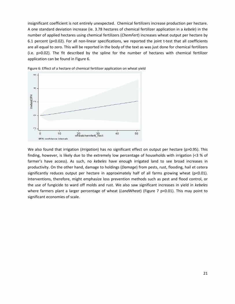
insignificant coefficient is not entirely unexpected. Chemical fertilizers increase production per hectare. A one standard deviation increase (ie. 3.78 hectares of chemical fertilizer application in a kebele) in the number of applied hectares using chemical fertilizers (ChemFert) increases wheat output per hectare by 6.1 percent (p<0.02). For all non-linear specifications, we reported the joint t-test that all coefficients are all equal to zero. This will be reported in the body of the text as was just done for chemical fertilizers (i.e. p>0.02). The fit described by the spline for the number of hectares with chemical fertilizer application can be found in Figure 6.

Figure 6: Effect of a hectare of chemical fertilizer application on wheat yield

We also found that irrigation (Irrigation) has no significant effect on output per hectare (p>0.95). This finding, however, is likely due to the extremely low percentage of households with irrigation (<3 % of farmer’s have access). As such, no kebeles have enough irrigated land to see broad increases in productivity. On the other hand, damage to holdings (Damage) from pests, rust, flooding, hail et cetera significantly reduces output per hectare in approximately half of all farms growing wheat (p<0.01). Interventions, therefore, might emphasize loss prevention methods such as pest and flood control, or the use of fungicide to ward off molds and rust. We also saw significant increases in yield in kebeles where farmers plant a larger percentage of wheat (LandWheat) (Figure 7 p<0.01). This may point to significant economies of scale.

21

Figure 7: Effect of % of land planted as wheat on yields

We found that higher yields in the previous season are correlated with increases in the current Meher season (lnwheatOPH_t-1). While this seems to be a relatively obvious result, it should be emphasized that the size of the coefficient is not that large. Therefore, we can posit that while productivity is influenced by historical forces, this is not the critical component as many of the other variables have a significant impact (at least measured by standardized variables). A one standard deviation (approximately 8.5) increase in the previous year’s output per hectare is related to an 8.8% increase in yields the year following (p<0.01). Put another way, a one unit increase in last year’s OPH has an approximate 0.17 OPH increase in the current output per hectare.

All of these effects are estimated holding critical environmental determinants constant. For instance, we control for elevation (Elev), slope (Slope), agroecological zones (AgroEco), edaphic properties (i.e., CEC), climatic water deficit (CWDMN), and precipitation (Precip). We also control for plant health through critical periods of the growing season through the use of the Enhanced Vegetation Index (EVI). EVIMAX correlates well with leaf area and total growth from establishment to the flowering period. EVID proxy’s plant health and water availability during the critical head development or ‘grain filling’ period. EVI maximum values (EVIMX) and area under the declining portion of the EVI curve of (EVID) both significantly correlates with output per hectare (p<0.06 and p<0.05, respectively). In the discussion below, the effects of these environmental variables are briefly outlined.

EVIMAX remains small and positive until very high levels and then dramatically decreases output per hectare (Figure 8). As such, EVIMAX is capturing increases in productivity due to total growth and leaf area until this declines with the wettest areas of the south, which have extremely high EVI values and low wheat productivity that were not properly screened out (as described in Section 3.1.4 Remotely Sensed Data).

22

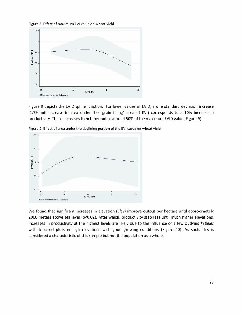
Figure 8: Effect of maximum EVI value on wheat yield

Figure 9 depicts the EVID spline function. For lower values of EVID, a one standard deviation increase (1.79 unit increase in area under the “grain filling” area of EVI) corresponds to a 10% increase in productivity. These increases then taper out at around 50% of the maximum EVID value (Figure 9).

Figure 9: Effect of area under the declining portion of the EVI curve on wheat yield

We found that significant increases in elevation (Elev) improve output per hectare until approximately 2000 meters above sea level (p<0.02). After which, productivity stabilizes until much higher elevations. Increases in productivity at the highest levels are likely due to the influence of a few outlying kebeles with terraced plots in high elevations with good growing conditions (Figure 10). As such, this is considered a characteristic of this sample but not the population as a whole.

23

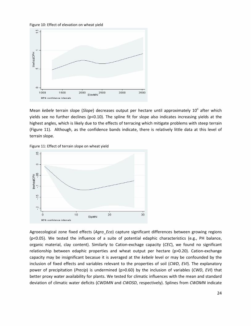
Figure 10: Effect of elevation on wheat yield

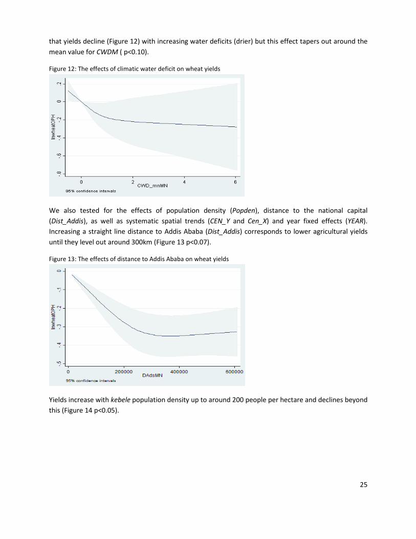
Mean kebele terrain slope (Slope) decreases output per hectare until approximately 10o after which yields see no further declines (p<0.10). The spline fit for slope also indicates increasing yields at the highest angles, which is likely due to the effects of terracing which mitigate problems with steep terrain (Figure 11). Although, as the confidence bands indicate, there is relatively little data at this level of terrain slope.

Figure 11: Effect of terrain slope on wheat yield

Agroecological zone fixed effects (Agro_Eco) capture significant differences between growing regions (p<0.05). We tested the influence of a suite of potential edaphic characteristics (e.g., PH balance, organic material, clay content). Similarly to Cation-exchage capacity (CEC), we found no significant relationship between edaphic properties and wheat output per hectare (p>0.20). Cation-exchange capacity may be insignificant becasue it is averaged at the kebele level or may be confounded by the inclusion of fixed effects and variables relevant to the properties of soil (CWD, EVI). The explanatory power of precipitation (Precip) is undermined (p>0.60) by the inclusion of variables (CWD, EVI) that better proxy water availability for plants. We tested for climatic influences with the mean and standard deviation of climatic water deficits (CWDMN and CWDSD, respectively). Splines from CWDMN indicate

24

that yields decline (Figure 12) with increasing water deficits (drier) but this effect tapers out around the mean value for CWDM ( p<0.10).

Figure 12: The effects of climatic water deficit on wheat yields

We also tested for the effects of population density (Popden), distance to the national capital (Dist_Addis), as well as systematic spatial trends (CEN_Y and Cen_X) and year fixed effects (YEAR). Increasing a straight line distance to Addis Ababa (Dist_Addis) corresponds to lower agricultural yields until they level out around 300km (Figure 13 p<0.07).

Figure 13: The effects of distance to Addis Ababa on wheat yields

Yields increase with kebele population density up to around 200 people per hectare and declines beyond this (Figure 14 p<0.05).

25

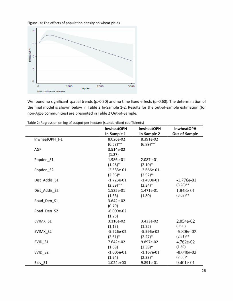
Figure 14: The effects of population density on wheat yields

We found no significant spatial trends (p>0.30) and no time fixed effects (p>0.60). The determination of the final model is shown below in Table 2 In-Sample 1-2. Results for the out-of-sample estimation (for non-AgSS communities) are presented in Table 2 Out-of-Sample.

Table 2: Regression on log of output per hectare (standardized coefficients)

lnwheatOPH In-Sample 1

lnwheatOPH In-Sample 2

lnwheatOPH Out-of-Sample

lnwheatOPH_t-1 8.026e-02 8.391e-02 (6.58)** (6.89)** AGP 3.514e-02 (1.27) Popden_S1 1.986e-01 2.087e-01 (1.96)* (2.10)* Popden_S2 -2.533e-01 -2.666e-01 (2.36)* (2.52)* Dist_Addis_S1 -1.723e-01 -1.490e-01 -1.776e-01 (2.59)** (2.34)* (3.28)** Dist_Addis_S2 1.525e-01 1.471e-01 1.848e-01 (1.56) (1.80) (3.02)** Road_Den_S1 3.642e-02 (0.79) Road_Den_S2 -6.009e-02 (1.25) EVIMX_S1 3.116e-02 3.433e-02 2.054e-02 (1.13) (1.25) (0.90) EVIMX_S2 -5.726e-02 -5.596e-02 -5.806e-02 (2.31)* (2.27)* (2.81)** EVID_S1 7.642e-02 9.897e-02 4.762e-02 (1.68) (2.38)* (1.39) EVID_S2 -1.005e-01 -1.167e-01 -8.040e-02 (1.94) (2.33)* (2.35)* Elev_S1 1.024e+00 9.891e-01 9.401e-01

26

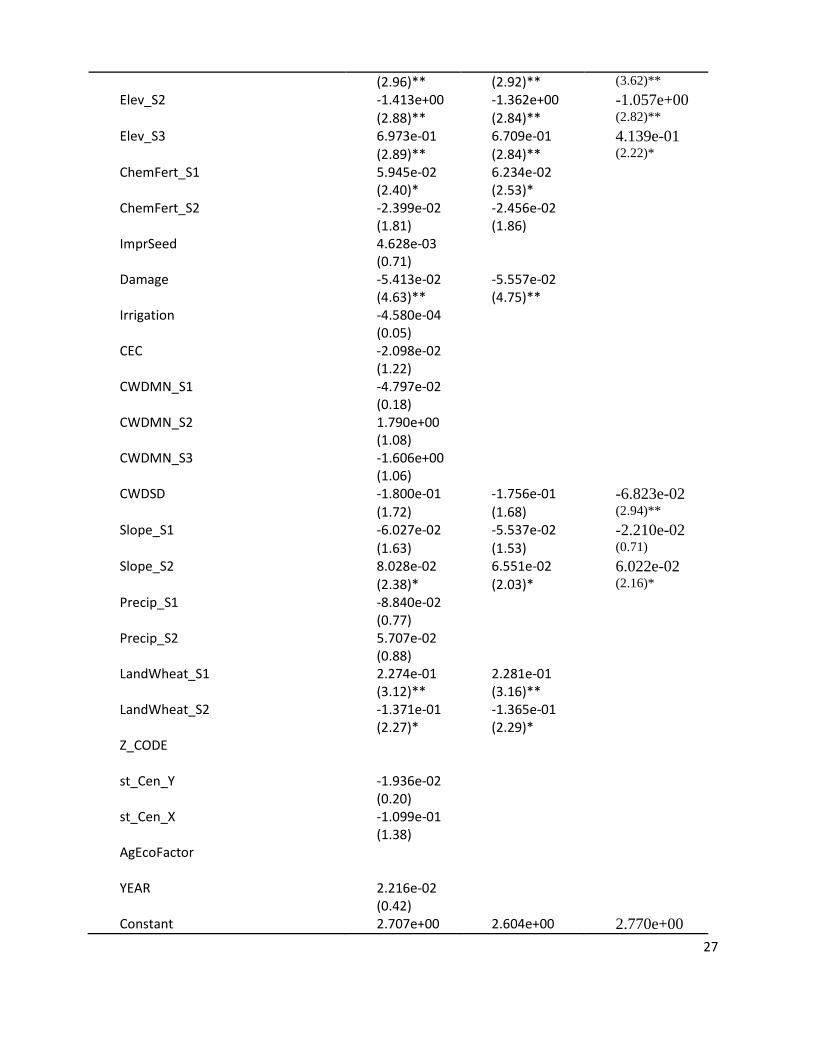
(2.96)** (2.92)** (3.62)** Elev_S2 -1.413e+00 -1.362e+00 -1.057e+00 (2.88)** (2.84)** (2.82)** Elev_S3 6.973e-01 6.709e-01 4.139e-01 (2.89)** (2.84)** (2.22)* ChemFert_S1 5.945e-02 6.234e-02 (2.40)* (2.53)* ChemFert_S2 -2.399e-02 -2.456e-02 (1.81) (1.86) ImprSeed 4.628e-03 (0.71) Damage -5.413e-02 -5.557e-02 (4.63)** (4.75)** Irrigation -4.580e-04 (0.05) CEC -2.098e-02 (1.22) CWDMN_S1 -4.797e-02 (0.18) CWDMN_S2 1.790e+00 (1.08) CWDMN_S3 -1.606e+00 (1.06) CWDSD -1.800e-01 -1.756e-01 -6.823e-02 (1.72) (1.68) (2.94)** Slope_S1 -6.027e-02 -5.537e-02 -2.210e-02 (1.63) (1.53) (0.71) Slope_S2 8.028e-02 6.551e-02 6.022e-02 (2.38)* (2.03)* (2.16)* Precip_S1 -8.840e-02 (0.77) Precip_S2 5.707e-02 (0.88) LandWheat_S1 2.274e-01 2.281e-01 (3.12)** (3.16)** LandWheat_S2 -1.371e-01 -1.365e-01 (2.27)* (2.29)* Z_CODE st_Cen_Y -1.936e-02 (0.20) st_Cen_X -1.099e-01 (1.38) AgEcoFactor YEAR 2.216e-02 (0.42) Constant 2.707e+00 2.604e+00 2.770e+00

27

(10.05)** (11.83)** (14.34)** R2 0.37 0.37 0.23 N 1,726 1,726 2,907

T-statistics in parentheses. * 95% level of significance, ** 99% level of significance

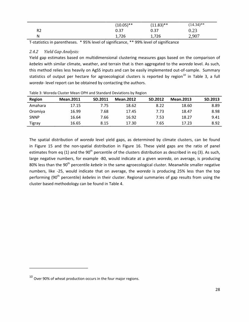
2.4.2 Yield Gap Analysis: Yield gap estimates based on multidimensional clustering measures gaps based on the comparison of kebeles with similar climate, weather, and terrain that is then aggregated to the woreda level. As such, this method relies less heavily on AgSS inputs and can be easily implemented out-of-sample. Summary statistics of output per hectare for agroecological clusters is reported by region10 in Table 3, a full woreda- level report can be obtained by contacting the authors.

Table 3: Woreda Cluster Mean OPH and Standard Deviations by Region

Region Mean.2011 SD.2011 Mean.2012 SD.2012 Mean.2013 SD.2013 Amahara 17.15 7.75 18.62 8.22 18.60 8.89 Oromiya 16.99 7.68 17.45 7.73 18.47 8.98 SNNP 16.64 7.66 16.92 7.53 18.27 9.41 Tigray 16.65 8.15 17.30 7.65 17.23 8.92

The spatial distribution of woreda level yield gaps, as determined by climate clusters, can be found in Figure 15 and the non-spatial distribution in Figure 16. These yield gaps are the ratio of panel estimates from eq (1) and the 90th percentile of the clusters distribution as described in eq (3). As such, large negative numbers, for example -80, would indicate at a given woreda, on average, is producing 80% less than the 90th percentile kebele in the same agroecological cluster. Meanwhile smaller negative numbers, like -25, would indicate that on average, the woreda is producing 25% less than the top performing (90th percentile) kebeles in their cluster. Regional summaries of gap results from using the cluster based methodology can be found in Table 4.

10 Over 90% of wheat production occurs in the four major regions.

28

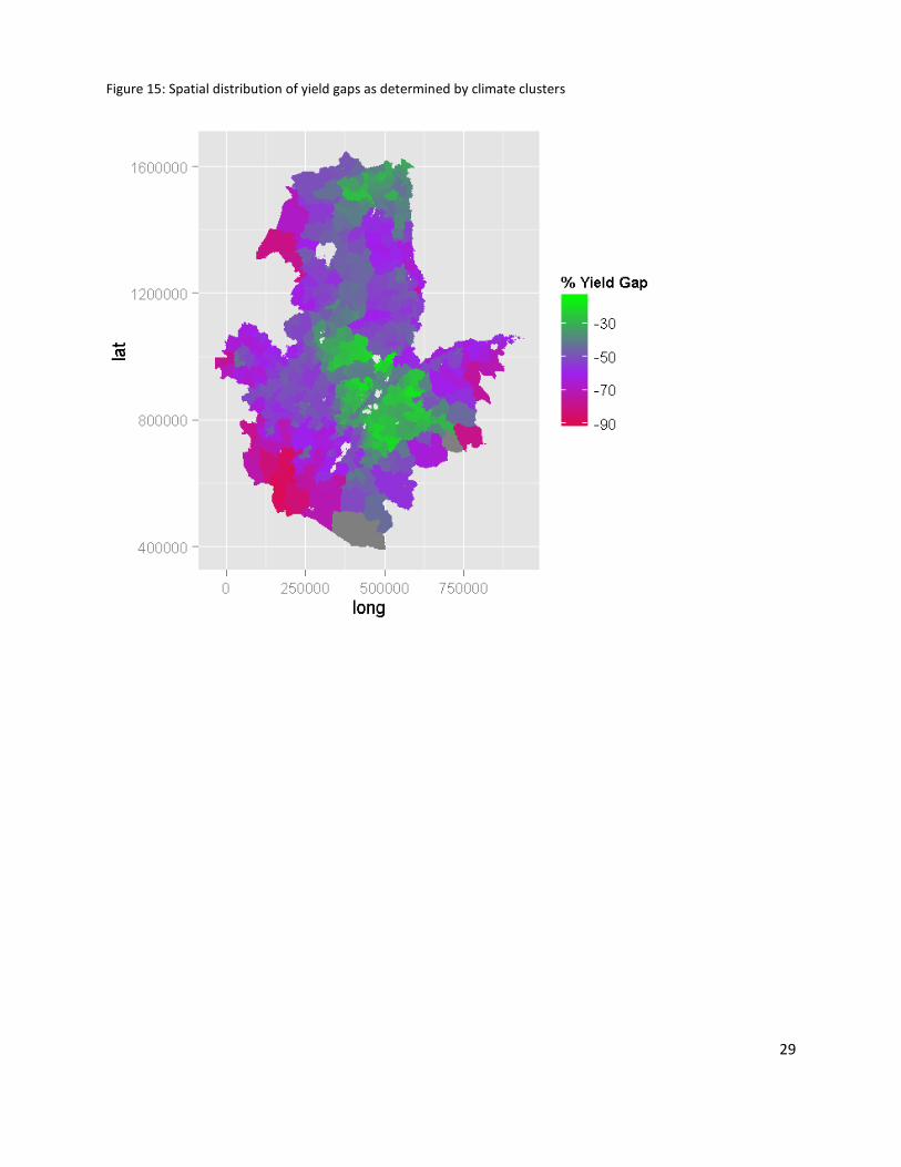
Figure 15: Spatial distribution of yield gaps as determined by climate clusters

29

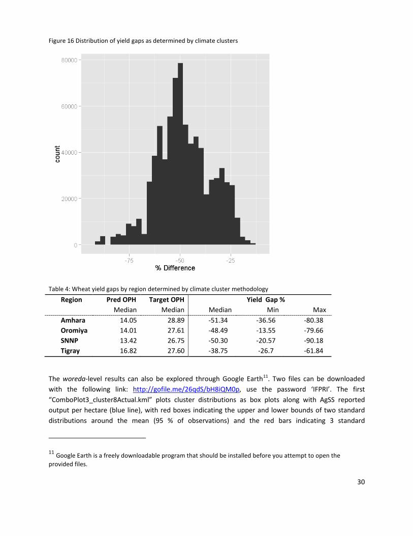
Figure 16 Distribution of yield gaps as determined by climate clusters

Table 4: Wheat yield gaps by region determined by climate cluster methodology

Region Pred OPH Target OPH Yield Gap % Median Median Median Min Max Amhara 14.05 28.89 -51.34 -36.56 -80.38 Oromiya 14.01 27.61 -48.49 -13.55 -79.66 SNNP 13.42 26.75 -50.30 -20.57 -90.18 Tigray 16.82 27.60 -38.75 -26.7 -61.84

The woreda-level results can also be explored through Google Earth11. Two files can be downloaded with the following link: http://gofile.me/26qdS/bH8iQM0p, use the password ‘IFPRI’. The first “ComboPlot3_cluster8Actual.kml” plots cluster distributions as box plots along with AgSS reported output per hectare (blue line), with red boxes indicating the upper and lower bounds of two standard distributions around the mean (95 % of observations) and the red bars indicating 3 standard

11 Google Earth is a freely downloadable program that should be installed before you attempt to open the provided files.

30

distributions (99%). “ComboPlot3_cluster8Estimate.kml” compares the cluster distribution with out-of-sample fixed effects estimates (orange line) estimated from equation (1).

2.5 Discussion

2.5.1 Panel Wheat Output per Hectare Results Given Ethiopia’s multi-cropping smallholder agriculture and the spatial heterogeneity of agro-ecological zones, the initial R-squares for wheat output per hectare of approximately 40% seem promising, and, we believe, justifies further development of this approach.

The Agricultural Growth Project (AGP), run by the Ministry of Agriculture and The World Bank, aims to increase agricultural productivity and market access for key crops and livestock products in targeted woredas (Policy & Bank, 2011). One of its two primary objectives is to increase agricultural yields for participating households. Controlling for other determinants in eq (1), we see a positive, yet statistically insignificant, increase in output per hectare for wheat (p<0.8). The coefficient estimates that AGP participating kebeles yields are 3.6% higher than non-AGP kebeles (for those kebeles both in the AgSS and AGP interventions), which is compared to the findings of the AGP baseline report of a 3.3% increase (IFPRI & EDRI, 2013). The high level of agreement between this study and the AGP baseline report lends credence to both the AgSS crop cut as well as the methods studied here. The statistical insignificance of this coefficient may reflect the ongoing nature of the AGP program and the particular intersection of the AgSS and AGP sample communities, rather than actual performance.

The AgSS also allows for the control of a variety of input and management relevant variables. We find that the self-reported application of improved seeds has no significant influence on wheat yields (p>0.40). While disappointing, the coefficients may not be significant for a variety of potential reasons. For example, there may not be widespread diffusion of those improved seeds most relevant to farmers’ challenges (e.g. rust resistant strains). It is advisable to, “Reduc[e] the area currently occupied by susceptible wheat varieties ... It is highly advisable to release and promote varieties that have durable adult plant resistance or have effective race-specific resistance genes in combinations to prevent further evolution and selection of new virulences that lead to boom-and-bust cycles of production” (Singh et al., 2011). This is echoed in the results on damages to agricultural holdings, where we find consistent and significant losses due to pests, rust, flooding and other risks to crops. For the 2012-2013 period, for instance, we find that 11% (3,948/35,844) of farmers and 9.3% (st. dev. = 20%) of all land planted experienced losses for one of these listed reasons. Interventions, therefore, might emphasize loss prevention methods such as pest and flood control, or the use of fungicide and improved seeds to ward off molds and rust. Finally, as previously mentioned, data collection methodology may underestimate actual improved seed use. As expected, chemical fertilizers significantly increase output per hectare. We find that the application of 3.7 additional hectares of chemical fertilizer in a kebele increases wheat production per hectare by 6.8%. This speaks to the significant gains that can be obtained through improved inputs and management. Although irrigation is likely a critical component of increasing and maintaining high productivity, we are currently unable to estimate its effects at the kebele level, which is likely due to the low percentage of households with access to even small-scale irrigation (less than 3% of households) and relatively good growing conditions for the sample period. That being said, the findings

31

of this report still point to a high level of sensitivity to changes in weather and climate. Irrigation, therefore, should and will play a significant role in food security and climate adaptation going forward. We also see significant increases in productivity from increasing the percentage of land devoted to wheat production. For a one standard deviation increase in the percentage of land planted (+12%) in wheat, we see a 25% increase in output per hectare. The government’s new cluster strategy may facilitate increased yields in the proposed wheat cluster areas. The relative importance of this variable should be tempered by its likely endogenous nature, with higher yields encouraging higher emphasis on wheat, and vice versa. That being said, this finding likely points to significant economies of scale for many suitable wheat producing regions, as increased scale brings with it lower input and transaction costs, and more capital investment, amongst others.

Year to year we see substantial volatility in the AgSS measures of output per hectare. One of the primary goals of this study was to evaluate whether or not these changes were due to measurement error or driven by the erratic nature of the small-scale rain-fed agricultural systems. In order to tease out potential weather-related effects, we control for a set of potential determinants of inter-annual variability. These time-variant controls include measures of rainfall, water availability, and plant health observed from satellites. We used measures of the enhanced vegetation index (see Section 3.1 Data and Methods for more detail) as a proxy for water availability and crop health at two critical periods of plant growth. The first, the area under the declining portion of the EVI curve, is a valuable measure of plant health and water availability through some of the most critical phases of head development and yield formation. With increases in EVID, we see substantial increases in productivity because of favorable conditions for plant growth. Here every one standard deviation increase (1.79 units) in EVID corresponds to a 10.4% increase in yields per hectare. This finding indicates that even in this challenging, small-scale heterogeneous environment, traditional satellite measures of plant health can be applied. It also suggests that despite favorable rains across much of the country during this period, there is substantial variation in productivity due to changes in water availability and, therefore, plant health. The slight declines in productivity (and substantial variability around these levels) for high levels of EVID may point to the effects of late rains, which increase the likelihood of molds and other diseases late in the growing season. The second EVI index, the maximum annual EVI value, is reached as the maximum levels of chlorophyll and leaf area are reached during the growing season. Here pixels with healthy productive plants with high leaf areas will have large maximum values. Alternatively pixels with a mixture of agricultural and non-agricultural vegetation will have very high EVI maximum values (see Figure 2: EVI Time series examples by land cover). Although productivity increases slightly with the EVI maximum, this variable more likely helps to screen out or penalize the productivity of pixels with a mixture of agricultural and non-agricultural lands. Looking at Figure 2, we can see that even wet agricultural areas rarely have maximum EVI values above 0.4. Looking at Figure 8, we can see that productivity declines rapidly in plots with EVI max values over this level. This is very likely because these pixels contain a higher percentage of tree cover. Additional processing of the data could reduce the noise associated with mixed EVI signatures.

We also include time-invariant measures of historical climate and climate variability, terrain characteristics, edaphic properties, and fixed effects indicators such as agroecological zones. Historical climate is proxied with the plant relevant metric of climatic water deficits, which provides a good

32

approximation of historical water availability. We see consistent declines in productivity in areas with historically high water deficits. Because CWD integrates information about precipitation along with soil characteristics and topography, it is a long-term indicator of conditions favorable for plant growth. For instance, sandy soils with steep slopes will likely have high CWD measures and be generally unfavorable for plant growth while flat loamy soils will likely have the opposite effect. As such, CWD likely captures some of the critical soils (edaphic) and terrain properties that were found insignificant in these regressions, such as CEC and a suite of other edaphic properties from AfriSIS data (e.g., pH balance, organic matter, clay content). Additionally, it is an indicator of climate expectations of farmers and will likely influence choices such as crop planting type. The inclusion of climatic variability (CWDSD) captures some of the effects of climate uncertainty on wheat productivity. Farmers in areas with higher variability in rainfall and relatively unfavorable soil and topographic characteristics (higher CWDSD) would be unlikely to make longer-term investments that might boost productivity. Significant fixed effects controls at the zonal and agroecological level speak to the effects of omitted variables, as well as the effects of policy choices and expected growing season length.

Topography, demographics, and distance to key cities also affect productivity. From Figure 10 and Figure 11 we can see that elevation enhances productivity up to a point. The specific relationship between productivity and elevation needs careful attention as the spline function indicates. While both extremely high elevation and increasing terrain slope decreases productivity, this need not be a death knell to productivity. This is likely a testament to the Ethiopian people as they terrace and plant in areas not traditionally suitable for agriculture. Even high elevations do not necessarily imply inhospitable climates and growing conditions (Ethiopia is a parable itself as it is one of the highest elevation crop producing countries in the world). Instead variation in topography and localized conditions in Ethiopia may allow for small pockets of rarified ideal conditions.

Beyond topography, the model explores some basic distance and population demographic effects. The model demonstrates that output productivity declines with greater distances from Addis Ababa (Figure 13). This finding likely speaks to the effects of limited access to inputs, investment and therefore capital accumulation. Productivity also varies according to population density with productivity initially increasing with population density, which is likely tied to improved access to inputs, labor, or capital, and declines thereafter as rural landscapes transition to more urban ones.

2.5.2 Yield Gap Results Yield gaps estimated by the ratio of eq (1) estimates and 90th percentile of kebeles in a climate cluster, mirrors the results from the in-sample methodology (see Appendix A). Looking at Table 4, we see substantial gaps between median woreda-level performances relative to the 90% kebeles in each climate cluster12. At the median, Oromiya and Tigray have the lowest gaps, averaging around 40% less than the top yielding kebeles in their climate clusters. The range of yield gaps is quite high, with some

12 Note that no woreda is producing at or above the 90th percentile kebele. This is because mean woreda productivity is being compared to the distribution of kebele productivity. Therefore, as discussed in the yield gap methodology section, mean woreda performance should be expected to lag behind top performing kebeles.

33

woredas in Oromiya producing between 79 and 13% less (on average) than the best performing kebeles. Potential variables driving these differences might be access to credit, inputs not included in this model, capital investment or agricultural extensions. Amhara and SNNP median gaps lag slightly behind, with median gaps around 50%. These results most likely reflect the difficult growing conditions in some of the areas. We see relatively smaller gaps in the central highlands centered around Addis Ababa and extending into central Oromia (Figure 15). This is the area typically considered the “wheat belt” that has benefited from some recent mechanization interventions. As seen in-sample, central to North West Tigray has higher productivity than other areas with similar climate, water availability, and terrain. The relative successes in Tigray points to potential power of agricultural interventions to broadly increase yields in Ethiopia, even in the most challenging environments.

The gap maps produced here can be used to evaluate the efficacy of ongoing interventions at an aggregate scale for the 2011-2013 period. Interventions in top performing woredas (green in Figure 15, and Appendix Figure A2) should be identified and likely emulated elsewhere. Policy makers might then target woredas with intermediate yield gaps, as they narrowly lag top performing areas. Looking at Figure 15, interventions might focus on woredas shown in dark purple allowing them to catch up to the better performing woredas. Successful interventions applied in top performing woredas will likely address pressing agricultural issues that we identified in the first section of this paper, such as addressing rusts and molds (Singh et al., 2011), improving access to fertilizer, and expanding irrigation in weather sensitive areas .

2.5.3 Model Improvements Moving forward, a number of improvements could be made to increase the accuracy of the models described here. First and foremost, models could be used with household-level productivity estimates. Aggregation at the kebele level, while highly desirable relative to woreda or zonal level estimates, obscure key sources variance that can be observed at only the farm or plot level. The inter-annual noise observed in AgSS crop cut data may be forced by causes other than measurement error. For instance, catastrophic losses due to disease or pests on even five of the 20 households sampled in the kebele could significantly decrease estimates. A more spatially explicit examination of the data may allow us to understand the determinants successful and unsuccessful years better. In lieu of household data sets, the inclusion of additional AgSS years could help differentiate real changes in productivity from noise.

The current model could also be augmented with additional spatial data. For instance, the 250m resolution MODIS data used in this study could be downscaled using the 30m Landsat products. This method would allow for the delineation of individual plot level attributes not currently distinguishable in this report. Additionally, improvements to core spatial data such as road maps, currently under development by the WLRC, will be a significant upgrade to currently available data (WLRC, 2013). The current soil sampling initiative, EthioSIS, led by both the Ministry of Agriculture and the Agricultural Transformation Agency, would be extremely valuable in augmenting productivity within this modeling structure. The development of an Ethiopia-specific land cover, land use product would also significantly contribute to the total area planted estimates, as well as the masking of non-agricultural signals.

34

The model could also be significantly improved by further collaboration with local and regional experts. This should include further discussions with local agronomists, policymakers, academics, as well as other economists. Additionally, the integration of crop growth models for the estimation of spatially explicit ‘potential yields’ could be used to enhance estimated gap models further.

2.5.4 Future Applications In order to create the initial EVI land use classes, a random sample of 200 pixels were chosen and then compared to high resolution Google Earth imagery for confirmation of actual terrain characteristics (eg. semi-arid, wet agriculture, see Figure 2). From this sample, a simplified methodology was created to determine basic land cover usages, primarily to roughly exclude non-agricultural lands. Carefully reexamining these methods could create more accurate land use maps. If coupled with higher resolution imagery, this analysis could provide land use maps at up to 30m resolution. Updating this map could provide a detailed look at the current land use patterns and could augment many types of agricultural research.

While the difficulty of creating this prototype was fairly time-consuming, creating this type of analysis for other crops could be done in a timely manner. Contrasting this model with other crops could also provide insight into varying crop management practices, weather-related impacts, as well as differing geophysical impacts based on crop types. This work could also confirm the overall applicability of the model.

As the last section indicated, downscaling the model to the field level (using greater resolution pixels or unmanned aerial vehicles (i.e. “drones”)) would provide insight into the determinants of productivity, and enhance accuracy that may have been lost in kebele-level aggregation. If coupled with field visits, this high-resolution look could explore crop specific attributes, management practices, as well as the farmers’ climate sensitivity. In other words, studying localized crop production would give the model the potential for better aggregation or a more detailed analysis in a smaller area, high value, crop applications (e.g.,. sesame cluster).

While there is much interest in climate change, much of it seems to be focused on studying changing annualized precipitation and temperature patterns. Even though precipitation is important to understand, metrics relevant to plant growth such as CWD and EVI integrate information about both water supply and demand. Considering the extreme heterogeneity of Ethiopia’s climate, soils, and terrain, integrating this information will likely prove critical to understanding Ethiopia’s climate history and future. Put simply, metrics like EVI capture current plant health given water availability while CWD could be used to estimate longer-term impacts of a changing climate. Together, these types of products could provide critical information for potential climate change impact (including variables such changes in plantable area, effects on productivity, shifts in species distribution, relative temperature changes as well as water availability).

A potential application of remote sensed products is for crop insurance interventions. For example, a cataloged historical EVI “greenness” index could be created at almost any scale at very low cost. If the current EVI drops below some acceptable reference level, then a possible insurance payment could be made. At the very least, this type of research could augment the typical adjuster’s evaluation.

35

While this work has been undertaken outside the scope of CSA’s data collection activities, integrating this data with CSA could better inform crop production and crop productivity estimates. While we are anecdotally aware that the CSA may be testing remote sensing for sampling design, some of the data presented here could be used in closer collaboration with national agricultural data collection.

An agricultural index could be created that measures the relative variability of agricultural potential within each woreda. Because the woreda is the basic unit for policy implementation, interventions could be better targeted with an improved understanding of how each woreda varies in terms of agricultural potential and risk. Looking at the model presented here, as an example, future studies should likely focus on the kebele as the unit of analysis. Kebeles provide a more homogenous unit of analysis (less variability in weather, soils, etc). Studies focusing at this level can, therefore, better capture the heterogeneity of the Ethiopian landscape.

These data techniques also necessitate a multidisciplinary approach. Understanding crop phenology, particularly within the context of the crop growing cycle, is important for productivity analysis. A better understanding of these cycles should help us differentiate specific crop types and their productivity remotely. Further, advancements of this methodology, within the context of interdisciplinary work between soil scientists, economists, geographers and others, will help us better understand and model these challenging local environments.

36

3. References

AGSS. (2013). Ethiopian Agricultural Sample Survey. Addis Ababa: Central Statistical Agency of Ethiopia. Retrieved from www.csa.gov.et/

Ahmad, I., Ghafoor, A., Muhammad Iftikhar Bhatti, M. I., Akhtar, I. H., Ibrahim, M., & Rehman, O. (2014). Satellite Remote Sensing and GIS based Crops Forecasting & Estimation System in Pakistan. Islamabad, Pakistan: Space Applications and Research Complex, Pakistan Space and Upper Atmosphere Research Commission. Retrieved from http://www.fao.org/fileadmin/templates/rap/files/Project/Expert_Meeting__17Feb2014_/P22_Satellite_Remote_Sensing_and_GIS_based_Crops_Forecasting___Estimation_System_in_Pakistan.pdf

Cliff, A., & Ord, J. (1981). Spatial Processes: models and applications. (Anonymous, Ed.). London: Pion.

Didan, K., & Huete, A. (2006). MODIS Vegetation Index Product Series Collection 5 Change Summary. Tucson, Arizona. Retrieved from https://lpdaac.usgs.gov/products/modis_products_table/mod13q1

FAO. (2013). Crop Water Information: Wheat. Retrieved from http://www.fao.org/nr/water/cropinfo_wheat.html

Ferenz, C. P., Bognar, J., Lichtenberger, D., Hamar, G., Tarcsai, G., Timar, G., … Ferencz-Arkos, I. (2004). Crop yield estimation by satellite remote sensing. International Journal of Remote Sensing, 25(20), 4113–4149.

GSFC. (2014). Tropical Rainfall Measurement Mission Project (TRMM) , Daily TRMM and Others Rainfall Estimate (3B42 V7 derived) , version 7 ,. Retrieved from http://disc.sci.gsfc.nasa.gov/recipes/?q=datacollection/TRMM_3B42_daily.007/description

Hausman, J. A. (1978). Specification tests in econometrics. Econometrica: Journal of the Econometric Society, 1251–1271.

Huber, P. (1967). The behavior of maximum likelihood estimates under nonstandard conditions. Proceedings of the Fifth Berkeley Symposium on Mathematical Statistics and Probability, 1, 221–233.

IFPRI. (2013). AGRICULTURAL GROWTH PROGRAM (AGP) OF ETHIOPIA - BASELINE REPORT 2011 - ESSP II. Washington DC.

IFPRI, & EDRI. (2013). AGRICULTURAL GROWTH PROGRAM (AGP) OF ETHIOPIA — BASELINE REPORT 2011 (p. 16). Addis Ababa.

37

Jarvis, A., Reuter, H. I., Nelson, A., & Guevara, E. (2008). Hole-filled SRTM for the globe Version 4, available from the CGIAR-CSI SRTM 90m Database. Retrieved from http://srtm.csi.cgiar.org

Kassie, B. T., Van Ittersum, M. K., Hengsdijk, H., Asseng, S., Wolf, J., & Rötter, R. P. (2014). Climate-induced yield variability and yield gaps of maize (Zea mays L.) in the Central Rift Valley of Ethiopia. Field Crops Research, 160, 41–53.

Lachenbruch, P., & Mickey, M. (1968). Estimation of error rates in discriminant analysis. Technometrics, 10(1), 1–12.

Leenaars, J. G. B. (2013). ISRIC report 2013/03. Africa Soil Profiles Database, Version 1.1. A compilation of geo-referenced and standardized legacy soil profile data for Sub Saharan Africa (with dataset). (W. ISRIC – World Soil Information the Netherlands., Ed.). Africa Soil Information Service (AfSIS) project. Retrieved from http://www.isric.org/data/africa-soil-profiles-database-version-01-1

Licker, R., Johnston, M., Foley, J., Barford, C., Kucharik, C., Monfreda, C., & Ramankutty, N. (2011). Mind the gap: how do climate and agricultural management explain the “yield gap” of croplands around the world? Global Ecol Biogeogr, 19, 769–782.

Liu, J., Liu, M., Tian, H., Zhuang, D., Zhang, Z., Zhang, W., … Deng, X. (2005). Spatial and temporal patterns of China’s cropland during 1990–2000: An analysis based on Landsat TM data. Remote Sensing of Environment, 98(4), 442–456. doi:http://dx.doi.org/10.1016/j.rse.2005.08.012

Lobell, D. B. J., Ortiz-Monasterio, J., G., A., Naylor, R., & Falcon, W. (2005). WHEAT—Combining Field Surveys, Remote Sensing, and Regression Trees to Understand Yield Variations in an Irrigated Wheat Landscape. Agronomy Journal, 97, 241–249.

Major, J. (1967). Potential evapotranspiration and plant distribution in western states with emphasis on California. AMER ASSOC ADVANCE SCI PUBL, 86(93-126).

Moran, M. S., Inoue, Y., & Barnes, E. M. (1997). Opportunities and limitations for image-based remote sensing in precision crop management. Remote Sensing of Environment, 61(3), 319–346. doi:http://dx.doi.org/10.1016/S0034-4257(97)00045-X

Nin-Pratt, A., Johnson, M., Magalhaes, E., You, L., Diao, X., & Chamberlin, J. (2011). Yield Gaps and Potential Agricultural Growth in West and Central Africa (pp. 1–158). Washington D.C.

Policy, M. of A., & Bank, T. W. (2011). ETHIOPIA - AGRICULTURAL GROWTH PROJECT (AGP) PROJECT INFORMATION DOCUMENT (PID).

Population Census Commission. (2008). Summary and Statistical Report of the 2007 Population and Housing Census: Population Size by Sex and Age. Addis Ababa, Ethiopia.

38

Prasad, A. K., Chai, L., Singh, R. P., & Kafatos, M. (2006). Crop yield estimation model for Iowa using remote sensing and surface parameters. International Journal of Applied Earth Observation and Geoinformation, 8(1), 26–33. doi:http://dx.doi.org/10.1016/j.jag.2005.06.002

Serrano, L., Filella, I., & Peñuelas, J. (2000, May). Remote Sensing of Biomass and Yield of Winter Wheat under Different Nitrogen Supplies. Retrieved from https://dl.sciencesocieties.org/publications/cs/abstracts/40/3/723

Singh, R. P., Hodson, D. P., Huerta-Espino, J., Jin, Y., Bhavani, S., Njau, P., … Govindan, V. (2011). The Emergence of Ug99 Races of the Stem Rust Fungus is a Threat to World Wheat Production. Annual Review of Phytopathology, 49, 465–481.

Sosa-Escudero, W., & Bera, A. K. (2008). Tests for unbalanced error-components models under local misspecification. Stata Journal, 8(1), 68–78. Retrieved from http://www.stata-journal.com/article.html?article=sg164_1

Swinton, S. M., & Lowenberg-Deboer, J. (2001). Global adoption of precision agriculture technologies: Who, when and why. In Proceedings of the 3rd European Conference on Precision Agriculture (pp. 557–562).

The World Bank. (2013). World Development Indicators: Country Level Data for Ethiopia. Retrieved from http://data.worldbank.org/country/ethiopia

Tittonell, P., & Giller, K. (2012). When yield gaps are poverty traps: The paradigm of ecological intensification in African smallholder agriculture. Field Crops Research, 143, 76–90.

UN-OCHA. (2014). Humanitarian Response COD-FOD Registry. Retrieved October 09, 2014, from http://www.humanitarianresponse.info/operations/ethiopia/dataset/ethiopia-admin-level-1-boundaries-admin-level-2-boundaries-admin-level-3

White, H. (1980). A heteroskedasticity-consistent covariance matrix estimator and a direct test for heteroskedasticity. Econometrica1, 48, 817–830.

Willmott, C. J., & Matsuura, K. (2001). Terrestrial Water Budget Data Archive: Monthly Time Series (1950 - 1999) Version 1.02. Retrieved from http://climate.geog.udel.edu/~climate/html_pages/README.wb_ts2.html

Willmott, C. J., Rowe, C. M., & Mintz, Y. (1985). Climatology of the Terrestrial Seasonal Water Cycle. Journal of Climatology, 5, 589–606.

WLRC. (2013). Ethio GIS 2 . (W. and L. R. Centre, Ed.). Addis Ababa. Retrieved from http://www.wlrc-eth.org/

39

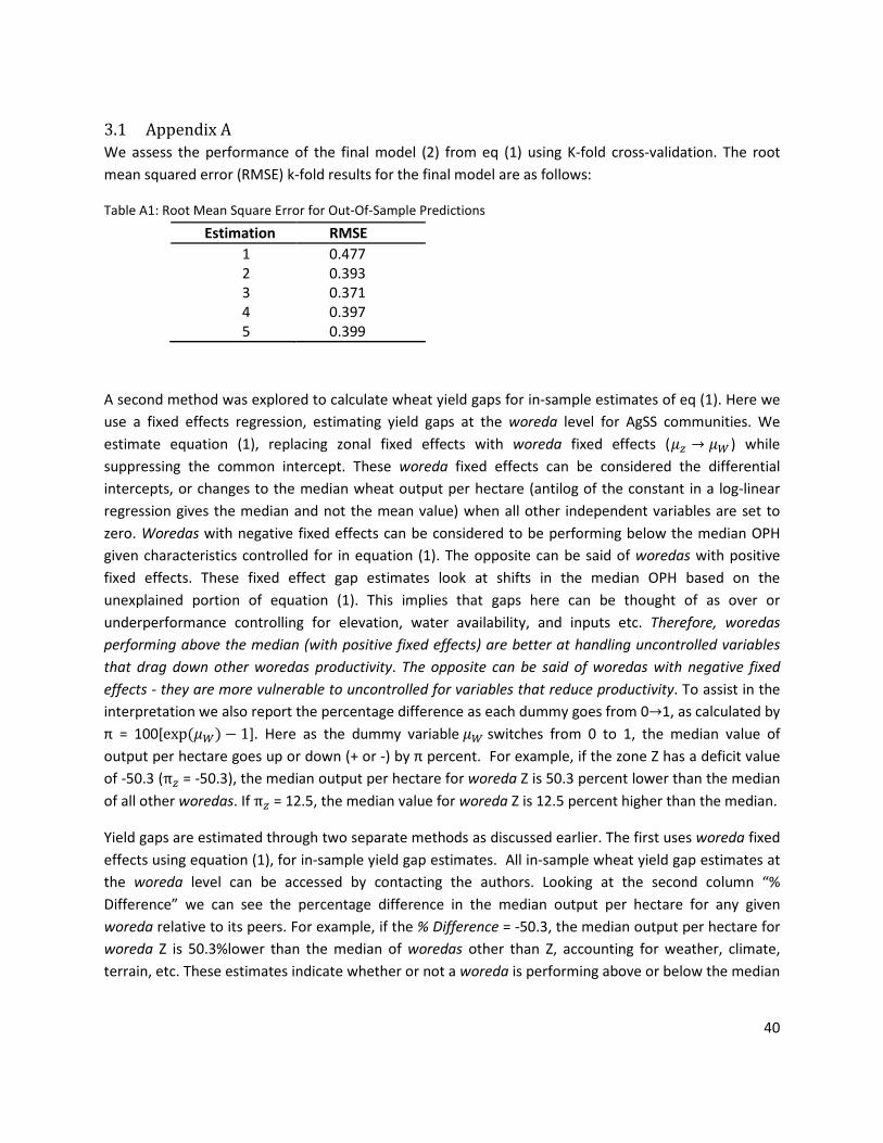
3.1 Appendix A We assess the performance of the final model (2) from eq (1) using K-fold cross-validation. The root mean squared error (RMSE) k-fold results for the final model are as follows:

Table A1: Root Mean Square Error for Out-Of-Sample Predictions

A second method was explored to calculate wheat yield gaps for in-sample estimates of eq (1). Here we use a fixed effects regression, estimating yield gaps at the woreda level for AgSS communities. We estimate equation (1), replacing zonal fixed effects with woreda fixed effects (𝜇𝜇𝑧𝑧 → 𝜇𝜇𝑊𝑊 ) while suppressing the common intercept. These woreda fixed effects can be considered the differential intercepts, or changes to the median wheat output per hectare (antilog of the constant in a log-linear regression gives the median and not the mean value) when all other independent variables are set to zero. Woredas with negative fixed effects can be considered to be performing below the median OPH given characteristics controlled for in equation (1). The opposite can be said of woredas with positive fixed effects. These fixed effect gap estimates look at shifts in the median OPH based on the unexplained portion of equation (1). This implies that gaps here can be thought of as over or underperformance controlling for elevation, water availability, and inputs etc. Therefore, woredas performing above the median (with positive fixed effects) are better at handling uncontrolled variables that drag down other woredas productivity. The opposite can be said of woredas with negative fixed effects - they are more vulnerable to uncontrolled for variables that reduce productivity. To assist in the interpretation we also report the percentage difference as each dummy goes from 0→1, as calculated by π = 100[exp (𝜇𝜇𝑊𝑊) − 1]. Here as the dummy variable 𝜇𝜇𝑊𝑊 switches from 0 to 1, the median value of output per hectare goes up or down (+ or -) by π percent. For example, if the zone Z has a deficit value of -50.3 (π𝑧𝑧 = -50.3), the median output per hectare for woreda Z is 50.3 percent lower than the median of all other woredas. If π𝑧𝑧 = 12.5, the median value for woreda Z is 12.5 percent higher than the median.

Yield gaps are estimated through two separate methods as discussed earlier. The first uses woreda fixed effects using equation (1), for in-sample yield gap estimates. All in-sample wheat yield gap estimates at the woreda level can be accessed by contacting the authors. Looking at the second column “% Difference” we can see the percentage difference in the median output per hectare for any given woreda relative to its peers. For example, if the % Difference = -50.3, the median output per hectare for woreda Z is 50.3%lower than the median of woredas other than Z, accounting for weather, climate, terrain, etc. These estimates indicate whether or not a woreda is performing above or below the median

Estimation RMSE 1 0.477 2 0.393 3 0.371 4 0.397 5 0.399

40

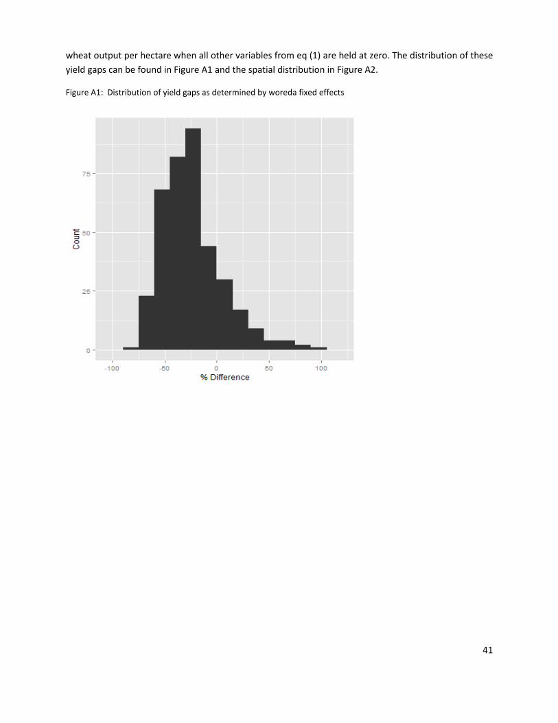
wheat output per hectare when all other variables from eq (1) are held at zero. The distribution of these yield gaps can be found in Figure A1 and the spatial distribution in Figure A2.

Figure A1: Distribution of yield gaps as determined by woreda fixed effects

41

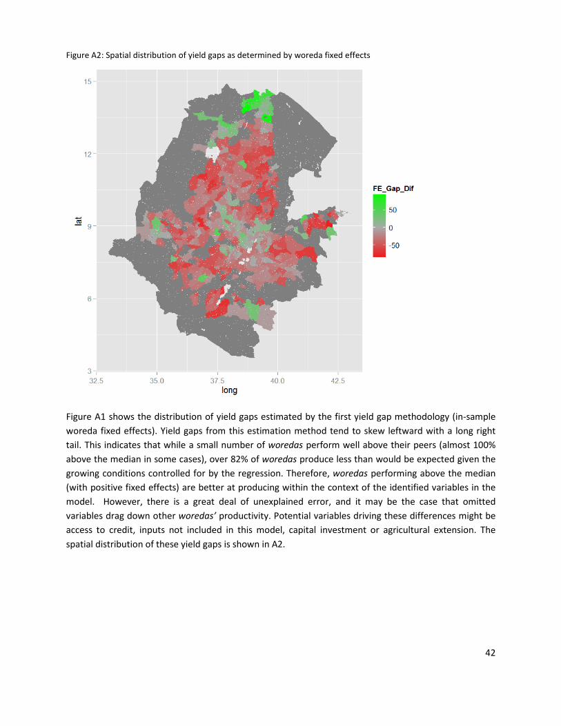
Figure A2: Spatial distribution of yield gaps as determined by woreda fixed effects

Figure A1 shows the distribution of yield gaps estimated by the first yield gap methodology (in-sample woreda fixed effects). Yield gaps from this estimation method tend to skew leftward with a long right tail. This indicates that while a small number of woredas perform well above their peers (almost 100% above the median in some cases), over 82% of woredas produce less than would be expected given the growing conditions controlled for by the regression. Therefore, woredas performing above the median (with positive fixed effects) are better at producing within the context of the identified variables in the model. However, there is a great deal of unexplained error, and it may be the case that omitted variables drag down other woredas’ productivity. Potential variables driving these differences might be access to credit, inputs not included in this model, capital investment or agricultural extension. The spatial distribution of these yield gaps is shown in A2.

42

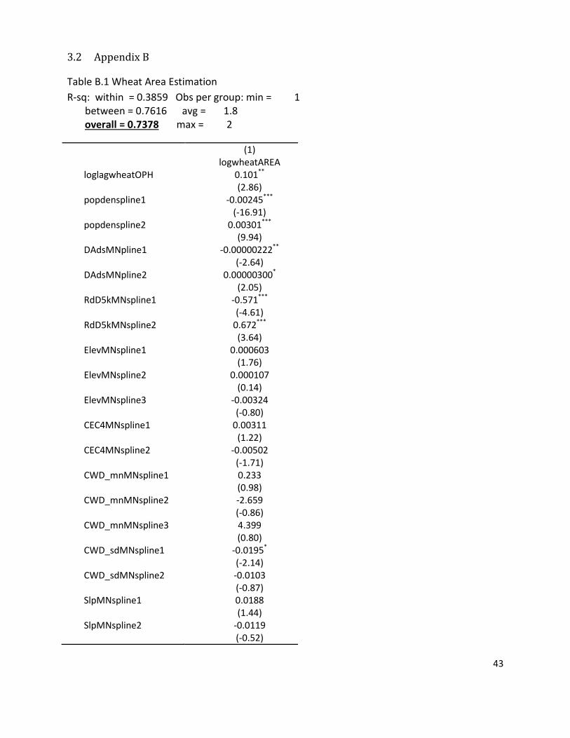
3.2 Appendix B

Table B.1 Wheat Area Estimation R-sq: within = 0.3859 Obs per group: min = 1 between = 0.7616 avg = 1.8 overall = 0.7378 max = 2

(1) logwheatAREA loglagwheatOPH 0.101** (2.86) popdenspline1 -0.00245*** (-16.91) popdenspline2 0.00301*** (9.94) DAdsMNpline1 -0.00000222** (-2.64) DAdsMNpline2 0.00000300* (2.05) RdD5kMNspline1 -0.571*** (-4.61) RdD5kMNspline2 0.672*** (3.64) ElevMNspline1 0.000603 (1.76) ElevMNspline2 0.000107 (0.14) ElevMNspline3 -0.00324 (-0.80) CEC4MNspline1 0.00311 (1.22) CEC4MNspline2 -0.00502 (-1.71) CWD_mnMNspline1 0.233 (0.98) CWD_mnMNspline2 -2.659 (-0.86) CWD_mnMNspline3 4.399 (0.80) CWD_sdMNspline1 -0.0195* (-2.14) CWD_sdMNspline2 -0.0103 (-0.87) SlpMNspline1 0.0188 (1.44) SlpMNspline2 -0.0119 (-0.52)

43

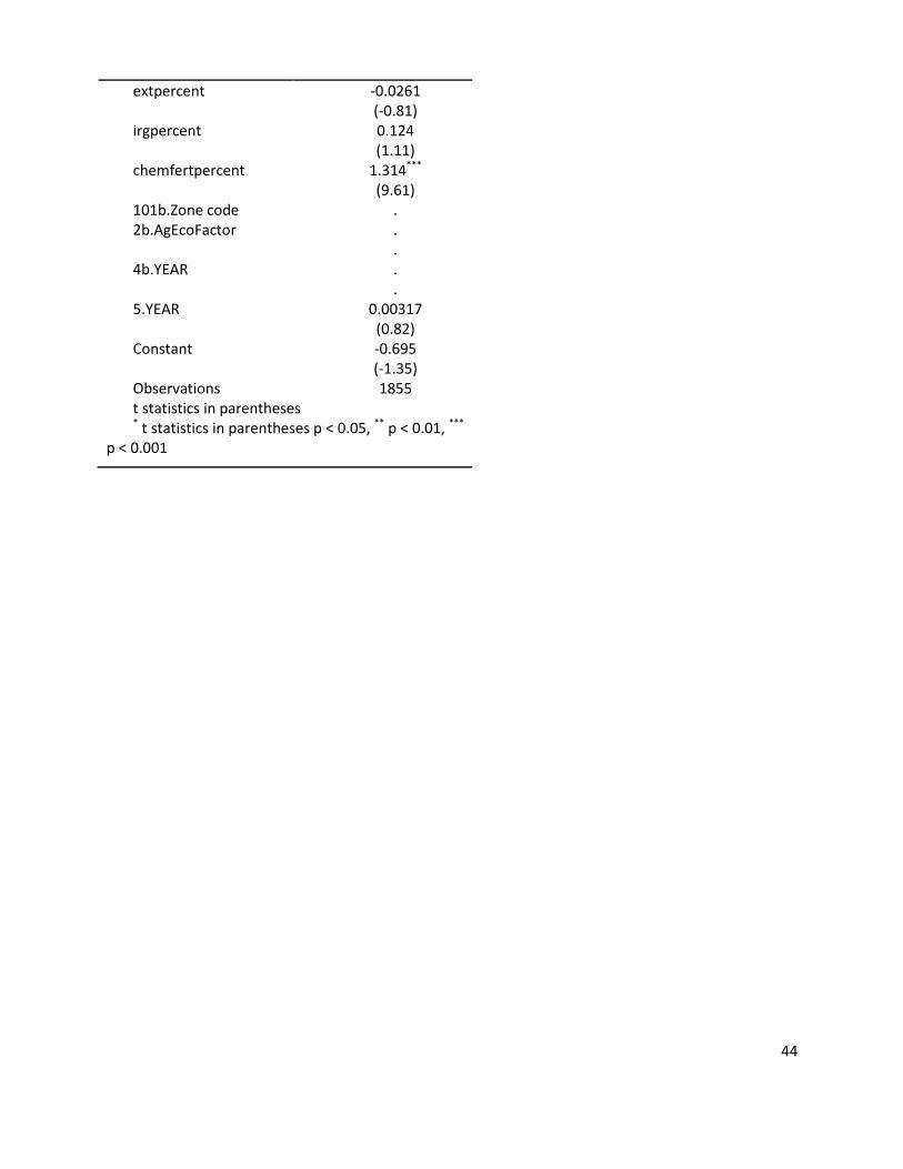
extpercent -0.0261 (-0.81) irgpercent 0.124 (1.11) chemfertpercent 1.314*** (9.61) 101b.Zone code . 2b.AgEcoFactor . . 4b.YEAR . . 5.YEAR 0.00317 (0.82) Constant -0.695 (-1.35) Observations 1855 t statistics in parentheses * t statistics in parentheses p < 0.05, ** p < 0.01, ***

p < 0.001

44