ET 2021 82 2

European Transport \ Trasporti Europei (2021) Issue 82, Paper n° 2, ISSN 1825-3997

https://doi.org/10.48295/ET.2021.82.2

Modelling of Activity-Travel Pattern with Support Vector Machine

Anu P. Alex 1, Manju V. S.2, Kuncheria P. Isaac3

1Associate Professor, College of Engineering Trivandrum, Kerala, India-695016 2Professor, College of Engineering Trivandrum, Kerala, India-695016

3Vice Chancellor, Hindustan Institute of Technology and Science, Chennai, India-603103 Abstract

Activity based travel demand modelling involves lot of uncertainty due to the complex and varying decision making behaviour of each individual. This study contributes to the literature by assessing the suitability of Support Vector Machine (SVM) in modelling the activity pattern and travel behaviour of workers. Activity and travel behaviour of workers consists of decision outcomes, which can be modelled as classification and regression problems. SVM is a good classifier and regressor with good testing and learning capability, hence the present study used SVM for modelling. It was found that support vector machine models are well performing to predict the activity pattern and travel behaviour of workers. The SVM models developed in the study predicts the temporal variation of mode wise work activity generation. Prediction of temporal mode share of commuters is advantageous to policy makers to experiment the implementation of temporary Travel Demand Management (TDM) actions effectively. Keywords: Transportation planning, mathematical modelling, Support Vector Machine, activity-travel pattern, activity based travel demand modelling

1. Introduction

The idea of demand and supply are elementary to economic theory and is extensively used in the field of transport economics. The concept could be applied in the area of travel demand and the supply of transport infrastructure. Modelling of demand implies a procedure for predicting the travel decisions of people. It is used to predict the future travel patterns and demands based on the changes in the transportation system, land use and demographic features. There are mainly two approaches in travel demand modelling; traditional statistically-oriented trip based modelling approach and more behaviourally-oriented activity-based modelling approach. The activity-based approach views travel as a derived demand; derived from the need to pursue activities distributed over space (Axhausen and Gärling, 1992; Kitamura, 1988; Pas, 1985). This approach concentrates on the chains of activities, with time segments as the analysis unit. By predicting what activities are performed when and where, activity based models forecast the trips, their timing and locations. The various approaches for activity-based modelling are Corresponding author: Anu P. Alex ([email protected])


2

constraints-based modelling, computational process modelling, micro simulation modelling and utility-maximizing models. The roots of constraints-based models are in time geography, whereas, computational process models are motivated by psychological decision process theories and utility-maximizing models are based on microeconomic theory (Timmermans et al. 2002). These studies exposed that activity based travel demand modelling involves lot of uncertainty due to the complex and varying decision making behaviour of each individual. The selection of modelling technique is very important due to this complexity. This leads to a research investigating the modelling of activity based travel demand using machine learning technique, which is very much fruitful to model the human behaviour. Machine learning paradigm, based on the theory of statistical learning, is a rapid advancement in data mining in recent decades. This has focussed engineering research towards modelling of natural phenomena in a realistic nature. Machine learning techniques can learn from data, identify patterns and make decisions with minimum human intervention. The iterative aspect of machine learning is very much important, since they learn from past computations, produce reliable and most accurate decisions. By developing precise models, the system has a better chance of avoiding unknown risks.

Support Vector Machine is a supervised machine learning technique, which has become extremely popular during the past years due to its applicability in classification and regression problems. Kernel trick is the major strength of SVM and it is not solved for local optima as in neural networks. The risk of overfitting is also less in SVM. This technique is successfully applied in various fields viz; protein structure prediction, intrusion detection, handwriting recognition, detecting steganography in digital images and breast cancer diagnosis. It has been successfully applied to model different civil and other engineering systems also (Dibike et al., 2001; Chuan and Yu, 2011; Yang and Zhao, 2013; Kim, 2014; Lam et al., 2010; Liu and Yao, 2017; Gui et al., 2017; Weng, 2018). In this context, the present study contributes to the literature by modelling the activity-travel pattern of workers using SVM, since this modelling consists of classification and regression problems, in which commuters decide the choices among outcomes and travel modes.

2. Activity-travel pattern of workers

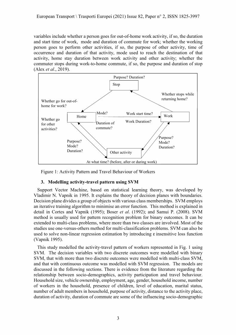
The study area selected to model the activity pattern and travel behaviour of workers is Thiruvananthapuram Corporation, the capital city of Kerala, the southernmost state in India. The city has considerable working population and they depend on public transport system and own vehicles to commute. Questionnaire survey was the main source of primary data collection. As it is not feasible to interview the whole population, sampling was resorted to. It was ensured that the sample was a true representation of the population. A total of 9530 persons were interviewed from 2521 households, which includes people from various socio-economic backgrounds. 41% of the sample population were workers, which included the employees in Government sector, private sector and self-employed. The distribution of activity-travel patterns of workers, obtained from the collected data, shows that 97.51% of the workers perform either ‘work activity only’ or ‘work activity + one other activity (before/ after/ during work or other activity stop during work to home commute)’ patterns. Hence, only these two activity-travel patterns of workers are modelled in this study. These two patterns are represented in Fig. 1. These patterns are modelled by identifying a number of decision variables as shown in Fig.1.The decision


3

Work

Other activity

Home Mode?

Duration of commute?

Whether go for out-of-home for work?

Whether go for other activities?

Purpose? Mode? Duration?

Purpose? Mode? Duration?

At what time? (before, after or during work)

Stop

Whether stops while returning home?

Purpose? Duration?

Work start time?

Work Duration?

variables include whether a person goes for out-of-home work activity, if so, the duration and start time of work, mode and duration of commute for work; whether the working person goes to perform other activities, if so, the purpose of other activity, time of occurrence and duration of that activity, mode used to reach the destination of that activity, home stay duration between work activity and other activity; whether the commuter stops during work-to-home commute, if so, the purpose and duration of stop (Alex et al., 2019).

Figure 1: Activity Pattern and Travel Behaviour of Workers

3. Modelling activity-travel pattern using SVM

Support Vector Machine, based on statistical learning theory, was developed by Vladimir N. Vapnik in 1995. It explains the theory of decision planes with boundaries. Decision plane divides a group of objects with various class memberships. SVM employs an iterative training algorithm to minimise an error function. This method is explained in detail in Cortes and Vapnik (1995); Boser et al. (1992); and Samui P. (2008). SVM method is usually used for pattern recognition problem for binary outcomes. It can be extended to multi-class problems, where more than two classes are involved. Most of the studies use one-versus-others method for multi-classification problems. SVM can also be used to solve non-linear regression estimation by introducing ε insensitive loss function (Vapnik 1995).

This study modelled the activity-travel pattern of workers represented in Fig. 1 using SVM. The decision variables with two discrete outcomes were modelled with binary SVM, that with more than two discrete outcomes were modelled with multi-class SVM, and that with continuous outcome was modelled with SVM regression. The models are discussed in the following sections. There is evidence from the literature regarding the relationship between socio-demographics, activity participation and travel behaviour. Household size, vehicle ownership, employment, age, gender, household income, number of workers in the household, presence of children, level of education, marital status, number of adult members in household, purpose of activity, distance to the activity place, duration of activity, duration of commute are some of the influencing socio-demographic


4

and activity based factors of activity participation and travel behaviour of individuals (Bhat, 2004; Yagi and Mohammadian, 2009). Variables with high correlations were eliminated and input parameters were finalized based on performance of the models. Notations used for influencing parameters, which are in the developed models are given in Table 1.

Table 1: Parameters and Notations

Notation Variables Notation Variables

H Household size mw Mode of commute for work

vo Vehicle ownership dc_w Duration of commute for work

g Gender pur_oth Purpose of other activities

ag Age group stop Whether stop during work-to-home commute

ms Marital status pur_stop Purpose of stop

emp Employment t_oth Time of occurrence of other activities

edu Level of education m_oth Mode used for other activities

HH Head of household d_oth Duration of other activities

wd Work duration st_oth Home stay duration

wst Work start time dur_stop Duration of stop

d Distance to work

3.1 Binary SVM A classification problem in binary is assessed with a group of training vectors (V) given

in Eq. (1), which belongs to two separate classes. 𝑉 = {(𝑥 , 𝑦 ), (𝑥 , 𝑦 ), … … … … … … … … . . , (𝑥 , 𝑦 )} (1) x ϵ RN,

Where x ϵ RN is an N-dimensional data vector with each sample belongs to either of the two classes, . The objective is to obtain a generalized classifier which can classify the two groups (-1, + 1) from the training set. In the current context of classifying decision variables, ‘selection of out-of-home work activity’ and ‘whether stop during work-to-home commute’, two classes were labeled as (-1, +1) and it means (yes, no). The ‘selection of out-of-home work activity’ depends on household size, vehicle ownership, employment, gender, marital status, age group, level of education, and whether the person is head of the household. ‘Whether stop during work-to-home commute’ depends on gender, marital status, mode of commute for work, duration of commute for work, distance to work place, age group, vehicle ownership, employment, level of education. So, x = [H, vo, g, ag, ms, emp, edu, HH] is the input data set used for selection of out-of-home work activity’ and x = [g, ms, mw, dw, d, ag, vo, emp, edu] is the data set used for ‘whether stop during work-to-home commute’. This means a linear hyper plane defined by Eq. (2) can classify the two classes of decision variables, where w ϵ Rn determines the orientation of the hyperplane and b ϵ R is a bias. Pictorial representation of a hyperplane is given in Fig. 2. 𝑓(𝑥) = 𝑤. 𝑥 + 𝑏 = 0 (2)


5

The separating hyperplane for the two classes can be defined as Eq. (3). 𝑦 (𝑤. 𝑥 + 𝑏) ≥ 1 − 𝜉 (for yi = 1, Yes) (3) 𝑦 (𝑤. 𝑥 + 𝑏) ≤ 1 − 𝜉 (for yi = -1, No)

Figure 2: Concept of SVM classification

Where, 𝜉 > 0 are slack variables, which are used to incorporate the effects of misclassification. The perpendicular distance between origin and the plane 𝑤. 𝑥 + 𝑏 =

−1 is | |

|| || and that to the plane 𝑤. 𝑥 + 𝑏 = 1 is

| |

|| ||. The margin (∂ (w,b)) between the

planes is given by (Eq(4)).

∂ (w,b) = || ||

(4)

The margin between two classes will be maximised and optimal hyperplane is located at the maximum (Fig. 2). Thereby error is minimized. This leads to the constrained optimization problem given in Eq. (5).

Minimize:𝑍 = |𝑤| + 𝐶 ∑ 𝜉 (5)

Subjected to: 𝑦 (𝑤. 𝑥 + 𝑏) ≥ 1 − 𝜉 The constant C, which lies between 0 and ∞, explains the transaction between the misclassifications in the training set and the maximization of margin. A large value of C minimizes error with lower generalization, whereas a small value of C minimizes error with higher generalization. When C goes to infinitely large, it results in a complex SVM model without allowing the occurrence of any error. If C goes to zero, the result would be less complex model with large amount of errors (Samui P., 2008). The optimization problem given in Eq (5) can be solved with following Lagrangian construction (Eq (6)) with multipliers α and β.

𝑤. 𝑥 + 𝑏= 0

𝑤. 𝑥 + 𝑏= −1

𝑤. 𝑥 + 𝑏= +1

𝑀𝑎𝑟𝑔𝑖𝑛 =2

||𝑤||

𝑆𝑢𝑝𝑝𝑜𝑟𝑡 𝑉𝑒𝑐𝑡𝑜𝑟𝑠


6

𝐿(𝑤, 𝑏, 𝛼, 𝛽, 𝜉) =|| ||

+ 𝐶 ∑ 𝜉 − ∑ 𝛼 {[(𝑤. 𝑥 + 𝑏)]𝑦 − 1 + 𝜉 } −

∑ 𝛽 𝜉 Lagrangian function has to be minimized with respect to w, b and ξ to obtain the saddle point. By differentiating L (w, b, α, β, ξ) with respect to w, band ξ and equating to zero, three conditions given in Eq. (7) were obtained:

𝜕𝐿(𝑤, 𝑏, 𝛼, 𝛽, 𝜉)

𝜕𝑤= 0, 𝑔𝑖𝑣𝑒𝑠 𝑤 = 𝛼 𝑦 𝑥

𝜕𝐿(𝑤, 𝑏, 𝛼, 𝛽, 𝜉)

𝜕𝑏= 0, 𝑔𝑖𝑣𝑒𝑠 𝛼 𝑦 = 0

𝜕𝐿(𝑤, 𝑏, 𝛼, 𝛽, 𝜉)

𝜕𝜉= 0, 𝑔𝑖𝑣𝑒𝑠 𝛼 + 𝛽 = 𝐶

Hence from Eqns. (6) and (7) the optimization problem can be expressed as in Eq. (8) (Osuna et al, 1997).

Maximize: 𝛼 − 1

2𝛼 𝛼 𝑦 𝑦 (𝑥 . 𝑥 )

𝑆𝑢𝑏𝑗𝑒𝑐𝑡𝑒𝑑 𝑡𝑜 ∶ 𝛼 𝑦 = 0 𝑎𝑛𝑑 0 ≤ 𝛼𝑖 ≤ 𝐶, 𝑖 = 1, 2, … … , 𝑁

Lagrange multipliers would be obtained by solving Eq. (8) with constraints. The multipliers may be non-zero or zero. Some of the multipliers will be zero according to the Karush–Kuhn–Tucker (KKT) optimality condition (Fletcher 1987). The non-zero multipliers are called support vectors, which are the data points lie on the optimal hyperplane and are difficult to classify. The values of w and b are obtained from 𝑤 =

∑ 𝑦 𝛼 𝑥 and 𝑏 = − 𝑤 [𝑥 + 𝑥 ], where x+1 and x-1 are the support vectors of

classes +1 (Yes) and -1 (No), respectively. The classifier can be formed as in Eq. (9): 𝑓(𝑥) = 𝑠𝑖𝑔𝑛(𝑤. 𝑥 + 𝑏) (9) Where sign (.) is the signum function. It gives -1 (No), if the element is less than zero and +1 (Yes), if it is greater than or equal to zero. If linear hyper plane is inappropriate, SVM maps input data into a high-dimensional feature space through some non-linear mapping (Boser et al. 1992). When x is replaced by its mapping in the feature space ϕ(x ), the optimization problem becomes Eq. (10).

Maximize: 𝛼 − 1

2𝛼 𝛼 𝑦 𝑦 (𝜙(𝑥 ), . 𝜙(𝑥 ))

Subjected to ∶ 𝛼 𝑦 = 0 𝑎𝑛𝑑 0 ≤ 𝛼𝑖 ≤ 𝐶, 𝑖 = 1, 2, … … , 𝑁

(8)

(6)

(7)


7

Instead of feature space 𝛷(𝑥 ), Kernel function 𝐾 𝑥 . 𝑥 = 𝛷(𝑥 ). 𝛷(𝑥 ) has been used to lessen computational requirement (Cristianini and Shawe-Taylor 2000; Cortes and Vapnik 1995). Radial basis function was used as kernel functions in the current study. The above discussed binary classification model was implemented in this study to model the decision outcomes of activity pattern and travel behaviour of workers. i.e; to predict whether a person goes for out-of-home work activity (yes/no) and to predict whether he/she stops during work to home commute (yes/no). The decision variables and classes are given in Table 2.

Table 2: Decision Variables and Outcomes of Binary SVM Models

Sl. No. Decision Variables Outcome Classes SVM Model Type

1 Whether go for out-of-home work activity

Yes No

+1 -1

Binary Classification

2 Whether stop during work-to-home commute

Yes No

+1 -1

Binary Classification

Separate training data and testing data sets were used for constructing and testing the performance of the models. Different values of hyper-parameters were tried and the parameters that yielded the best accuracy on the models were used. The hyper-parameters which gave better cross validation results and minimum number of support vectors were capacity constant, C= 10 and epsilon = 0.10. Kernel function used for transferring the data points to feature space was Radial Basis Function (RBF). The input parameters which gave better validation results were also selected by trial and error. The selected input parameters are shown in Table 4.

3.2 Multi-Class SVM

Higher level multi-class SVM methods are usually used for more than two classes, which utilizes binary classification as the basics. ‘One-versus-others method’ was used in this study. It is an effective and simple method for multi-class classification problems (Dubchak et al., 1999). Assume there are M classifications in the problem. It is converted into a binary classification problem, i.e; one class contains datapoints in one ‘true’ class and the ‘others’ class combines data in all other categories. A binary classifier is trained for this two-class problem. Then the M classes are partitioned into another binary classification problem. The same process is replicated for each of the M classes, which results in M binary trained classifiers.

Multi-class SVM method is used in the present study to model the decision variables with more than two outcomes. i.e: to predict the mode of commute for work, purpose of other activities, time of occurrence of other activities, mode used for other activities and purpose of stop. The decision variables and classes used for each are given in Table 3. As in binary classification, a training data set and testing data set were used for constructing and testing the models. The hyper-parameters which gave better cross validation results and minimum number of support vectors were capacity constant, C= 10 and epsilon = 0.10. Kernel function used for transferring the data points to feature space was Radial Basis Function (RBF). The input parameters which gave better validation results are shown in Table 4.

(10)


8

Table 3: Decision Variables and Outcomes of Multi-class SVM Models

Sl. No. Decision Variables Outcome Classes SVM Model Type

1 Mode of commute for work

Walk / cycle Two wheeler Car Bus Train

0 1 2 3 4

Multi-class SVM

2 Purpose of other activity

No activity Personal business and recreation Shopping Eat out

0 1 2 3

Multi-class SVM

3 Purpose of stop Care for children/spouse/elderly Shopping Personal business and recreation

0 1 2

Multi-class SVM

4 Time of occurrence of other activities

Before work After work Work based

0 1 2

Multi-class SVM

5 Mode used for other activities

Walk / cycle Two wheeler Car Bus

0 1 2 3

Multi-class SVM

Table 4: Input Variables and Performance of SVM Models

Sl. No

Attributes Input Variables Training Perf. (%)

Testing Perf. (%)

1 Whether go for out-of-home work activity

H, vo, g, ag, ms, emp, edu, HH 99.23 97.15

2 Work duration H, vo, g, ag, ms, emp, edu 82.35 81.65

3 Work start time wd, g, ag, edu 88.42 87.11

4 Mode of commute for work vo, g, ag, ms, emp, HH, wd, wst 73.25 70.41

5 Duration of commute for work wd, wst, d, vo, g, ag, emp, mw 75.36 74.13

6 Purpose of other activities wd, dc_w, d, H, vo, emp, mw, HH, edu, ag, g, ms

75.80 74.25

7 Whether stop during work-to-home commute

g, ms, mw, dc_w, d, ag, vo, emp, edu 95.12 94.47

8 Purpose of stop dc_w, emp, ag, H, g, ms 92.45 91.26

9 Time of occurrence of other activities

wd, wst, vo, ms, emp, edu, mw, pur_oth

85.28 84.89

10 Mode used for other activities vo, g, ag, pur_oth, t_oth 75.87 73.57

11 Duration of other activities wd, pur_oth, m_oth, t_oth 84.76 83.14

12 Home stay duration t_oth, wst, dc_w, pur_oth, H, wd, vo, g, d_oth, mw, emp, ag, ms

82.51 81.90

13 Duration of stop wd, dc_w, d, vo, g, ag, edu, pur_stop 90.52 89.48


9

3.3 SVM Regression The dependence of a variable y on a set of independent variables x can be estimated in SVM regression using an alternative loss function (Smola, 1996). Regression estimates are found out by a set of linear functions. These linear functions are defined in a high dimensional space in the first phase (Samui, P., 2008). Using Vapnik’s ε-insensitive loss function, risk is measured and it is minimized in the second step for carrying out estimation of regression. In the third step, regression SVM uses a risk function, which consists of a regularization term and empirical error. It is obtained from structural risk minimization (SRM) principle (Samui P., 2008). The concept of SVM regression is shown in Fig. 3.

Figure 3: Concept of SVM Regression

Assume that the dataset consists of{(𝑥 , 𝑦 ), (𝑥 , 𝑦 ), … … … … … … … … . . , (𝑥 , 𝑦 )}, where, 𝑥 is the input and 𝑦 is the output. Let us assume alinear function Eq. (11). 𝑓(𝑥) = (𝑤. 𝑥) + 𝑏 (11) where, w ϵ RN and b ϵ r; RN = N-dimensional vector space; b= scalar threshold; w = adjustable weight vector; and r = one dimensional vector space. The objective of SVM regression is to find a function 𝑓(𝑥) that gives a difference ε from the true output (y). The optimization problem involves Eq. (12) and (13):

Minimize: 𝑍 = |𝑤| + 𝐶 ∑ (𝜉 + 𝜉∗) (12)

Subjected to: 𝑦 − {(𝑤. 𝑥 + 𝑏)} ≤ 𝜀 + 𝜉 , 𝑖 = 1, 2, 3, … … … … 𝑁 {(𝑤. 𝑥 + 𝑏)} − 𝑦 ≤ 𝜀 + 𝜉 , 𝑖 = 1, 2, 3, … … … … 𝑁

𝜉 ≥ 0 𝑎𝑛𝑑 𝜉∗ ≥ 0 , 𝑖 = 1, 2, 3, … … … … 𝑁

The optimization problem given in Eq. (12) can be solved with the following Lagrangian construction (Eq (14)) with multipliers α, α*, γ and γ*.

𝐿(𝑤, 𝜉, 𝜉∗, 𝛼, 𝛼∗, 𝛾, 𝛾∗) =|𝑤|

2+ 𝐶[ (𝜉 + 𝜉∗)] − 𝛼 [𝜀 + 𝜉 − 𝑦 + (𝑤. 𝑥 + 𝑏)]

− ∑ 𝛼∗[𝜀 + 𝜉∗ + 𝑦 − (𝑤. 𝑥 ) − 𝑏] − ∑ 𝛾 𝜉 + 𝛾∗ 𝜉∗ (14)

(13)

+ε

-ε

ξ

y

x


10

Lagrangian function has to be minimized with respect to w, b, ξ and ξ* to obtain the saddle point. By differentiating 𝐿(𝑤, 𝜉, 𝜉∗, 𝛼, 𝛼∗, 𝛾, 𝛾∗) with respect to w, b, ξ and ξ* and equating to zero, the following four conditions were obtained Eq. (15):

= 0, 𝑔𝑖𝑣𝑒𝑠 𝑤 = ∑ 𝑥 (∝ −∝∗)

𝜕𝐿

𝜕𝑏= 0, 𝑔𝑖𝑣𝑒𝑠 ∝ = ∝∗

𝜕𝐿

𝜕𝜉= 0, 𝑔𝑖𝑣𝑒𝑠 𝛾 = (𝐶 −∝ )

𝜕𝐿

𝜕𝜉∗ = 0, 𝑔𝑖𝑣𝑒𝑠 𝛾𝑖 ∗

𝑁

𝑖=1

= (𝐶 −∝𝑖∗)

𝑁

𝑖=1

Hence from Eqs. (14) and (15) the optimization problem becomes Eq. (16) and (17):

𝑀𝑎𝑥𝑖𝑚𝑖𝑧𝑒: −𝜀 ∑ (𝛼∗ + 𝛼 ) + ∑ 𝑦 (𝛼∗ − 𝛼 ) − ∑ ∑ (𝛼∗ −

𝛼 )((𝛼∗ − 𝛼 )(𝑥 . 𝑥 )

Subjected to ∶ ∑ 𝛼 = ∑ 𝛼∗ , 0 ≤ 𝛼 ≤ 𝐶, 𝑎𝑛𝑑 0 ≤ 𝛼∗ ≤ 𝐶 𝑖 = 1, 2, … … , 𝑁 The coefficients α and α∗ can be found out by resolving the optimization problem in Eq. (16). Zero Lagrange multipliers means sparseness in the training objects. Training objects with non-zero Lagrange multipliers are the support vectors. Prediction errors of these objects will be larger than ±ε. In the case of inappropriateness of linear hyper plane, some non-linear mapping is done in SVM, where input data is mapped into a high-dimensional feature space (Boseret al. 1992). Optimization problem becomes Eq. (18) and (19), when feature space 𝜙(𝑥 ) replaces x by its mapping.

Maximize: −𝜀 (𝛼∗ + 𝛼 ) + 𝑦 (𝛼∗ − 𝛼 )

− 1

2(𝛼∗ − 𝛼 )((𝛼∗ − 𝛼 )(𝛷(𝑥 ). 𝛷(𝑥 ))

Subjected to ∶ 𝛼 = 𝛼∗ , 0 ≤ 𝛼𝑖 ≤ 𝐶, 𝑎𝑛𝑑 0 ≤ 𝛼𝑖 ∗ ≤ 𝐶 𝑖

= 1, 2, … … , 𝑁 Kernel function𝐾 𝑥 . 𝑥 = 𝛷(𝑥 ). 𝛷(𝑥 )is introduced as a replacement for feature space 𝛷(𝑥 ) to lessen the computational requirement (Cortes and Vapnik 1995; Cristianini and Shawe-Taylor 2000). Fig. 4 shows the architecture of SVM regression.

(15)

(17)

(16)

(18)

(19)


11

Figure 4: Architecture of SVM Regression

The above discussed SVM regression model was applied in this study to model the work duration, work start time, duration of commute for work, duration of other activities, home stay duration and duration of stop. A training data set and testing data set are used for constructing the model and testing the performance. The hyper-parameters which gave better cross validation results and minimum number of support vectors were capacity constant, C= 10 and epsilon = 0.10. Kernel function used was Radial Basis Function (RBF). The input parameters which gave better validation results are shown in Table 4.

4. Results and discussion

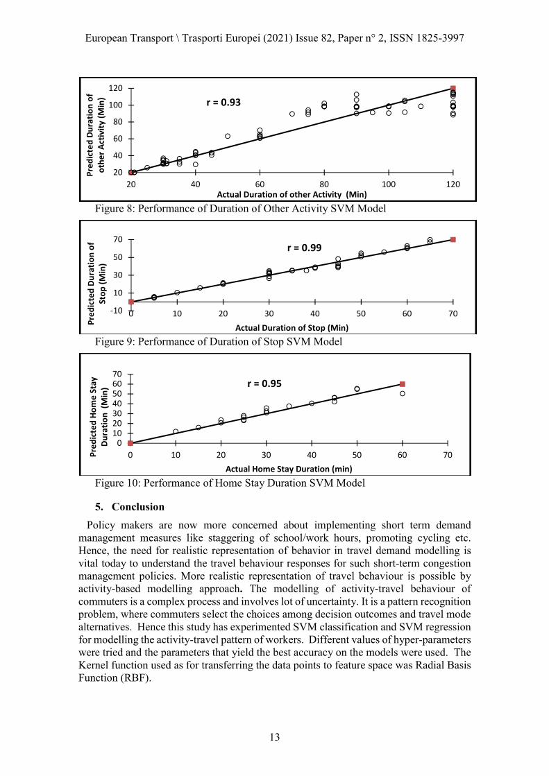
Model performances are represented in terms of training performance and testing performance in SVM models. The training and testing performance of the classification models are found out using Eq. (20) and those of regression models are calculated using Eq. (21). Table 4 represents the performance of the models. Higher training and testing performance shows that the models are good. The SVM classification and regression models were validated, to evaluate their performance, with new set of data, which are not used for training. The performance of the SVM classifications models, given in Table 5, shows that the prediction accuracy of the SVM classification models are above 70%. The performance of regression models are shown in Figs. 5 to 10, in which actual and predicted values are plotted. The correlation coefficient (r) obtained in all the cases are greater than 0.90. Hence it is proved that the developed models are capable of predicting the activity-travel pattern of workers. This is due to the training and learning capability of SVM. Training or Testing performance (%) 𝑜𝑓 𝑐𝑙𝑎𝑠𝑠𝑖𝑓𝑖𝑐𝑎𝑡𝑖𝑜𝑛 𝑚𝑜𝑑𝑒𝑙𝑠

=𝑁𝑢𝑚𝑏𝑒𝑟 𝑜𝑓 𝑑𝑎𝑡𝑎 𝑝𝑟𝑒𝑑𝑖𝑐𝑡𝑒𝑑 𝑎𝑐𝑐𝑢𝑟𝑎𝑡𝑒𝑙𝑦

𝑇𝑜𝑡𝑎𝑙 𝑛𝑢𝑚𝑏𝑒𝑟 𝑜𝑓 𝑑𝑎𝑡𝑎∗ 100

(20)

𝑥

𝑥

𝑥

𝑥

𝐾(𝑥, 𝑥 )

𝐾(𝑥, 𝑥 )

𝐾(𝑥, 𝑥

𝐾(𝑥, 𝑥 )

𝑓(𝑥)= (𝑤. 𝑥) + 𝑏

𝑦

Input Hidden Layer of

Bias

Output


12

Training or Testing performance (%) 𝑜𝑓 𝑟𝑒𝑔𝑟𝑒𝑠𝑠𝑖𝑜𝑛 𝑚𝑜𝑑𝑒𝑙𝑠

= 100 −𝐴𝑐𝑡𝑢𝑎𝑙 𝑣𝑎𝑙𝑢𝑒 − 𝑃𝑟𝑒𝑑𝑖𝑐𝑡𝑒𝑑 𝑉𝑎𝑙𝑢𝑒

𝐴𝑐𝑡𝑢𝑎𝑙 𝑉𝑎𝑙𝑢𝑒∗ 100

Table 5: Results of Validation of SVM Classification Models

Attributes Sample Size SVM Models

Correctly Predicted Prediction Accuracy (%)

Whether go for out-of-home work activity 777 753 96.88

Mode of commute for work 700 494 70.57

Purpose of other activities 700 523 74.67 Whether stop during work-to-home commute

700 650 92.87

Purpose of stop 306 281 91.89 Time of occurrence of other activities 259 215 83.12

Mode used for other activities 259 189 73.12

Figure 5: Performance of Work Duration SVM Model

Figure 6: Performance of Work Start Time SVM Model

Figure 7: Performance of Duration of Commute for Work SVM Model

350

400

450

500

550

600

350 400 450 500 550 600

Pred

icte

d W

ork

Dur

atio

n (M

in)

Actual Work Duration (Min)

01020304050

0,00 10,00 20,00 30,00 40,00 50,00

Pred

icte

d Co

mm

ute

Dur

atio

n (M

in)

Actual Commute Duration (Min)

r = 0.92

350

400

450

500

350 370 390 410 430 450 470 490

Pred

icte

d W

ork

Star

t Ti

me

(Min

)

Actual Work Start Time (Min)

r = 0.94

(21)


13

Figure 8: Performance of Duration of Other Activity SVM Model

Figure 9: Performance of Duration of Stop SVM Model

Figure 10: Performance of Home Stay Duration SVM Model

5. Conclusion

Policy makers are now more concerned about implementing short term demand management measures like staggering of school/work hours, promoting cycling etc. Hence, the need for realistic representation of behavior in travel demand modelling is vital today to understand the travel behaviour responses for such short-term congestion management policies. More realistic representation of travel behaviour is possible by activity-based modelling approach. The modelling of activity-travel behaviour of commuters is a complex process and involves lot of uncertainty. It is a pattern recognition problem, where commuters select the choices among decision outcomes and travel mode alternatives. Hence this study has experimented SVM classification and SVM regression for modelling the activity-travel pattern of workers. Different values of hyper-parameters were tried and the parameters that yield the best accuracy on the models were used. The Kernel function used as for transferring the data points to feature space was Radial Basis Function (RBF).

20

40

60

80

100

120

20 40 60 80 100 120

Pred

icte

d D

urat

ion

of

othe

r Act

ivity

(Min

)

Actual Duration of other Activity (Min)

r = 0.93

-10

10

30

50

70

0 10 20 30 40 50 60 70

Pred

icte

d D

urat

ion

of

Stop

(Min

)

Actual Duration of Stop (Min)

r = 0.99

010203040506070

0 10 20 30 40 50 60 70Pred

icte

d H

ome

Stay

D

urat

ion

(Min

)

Actual Home Stay Duration (min)

r = 0.95


14

The present study contributes to the literature by developing support vector machine models for activity-travel pattern. It is proved that SVM classification and regression models developed for predicting the activity-travel pattern of workers are well performing. The prediction accuracy of SVM classification models are more than 70% and SVM regression models gave good results (r> 0.90). This is due to the training capability and learning ability of SVM. The study proves that SVM is a powerful tool for modelling the activity pattern and travel behaviour of workers. Even though statistical check is not possible for SVM models, it is easy to transfer the model. It can be concluded from the study that the developed SVM models represent real life activity-travel pattern of workers. Hence it can be used for predicting the activity-travel pattern and thereby the modes used by workers. This will eventually help to analyse the temporal mode share of workers.

References

Alex, A.P., Manju V. S., Isaac, K. P. (2019) “Modelling of Travel Behaviour of Students using Artificial Intelligence”, Archives of Transport, Vol. 51. Issue 3, pg: 7 – 19. doi: 10.5604/01.3001.0013.6159

Axhausen, K. and Gärling, T. (1992) “Activity-based approaches to travel analysis: conceptual frameworks, models and research problems”, Transport Reviews, 12, 324-341.doi:10.1080/01441649208716826

Boser B. E., Guyon I. M., Vapnik V. N. (1992) “A training algorithm for optimal margin classifier” In: Proceedings of the Fifth Annual ACM Workshop on Computational Learning Theory, Pittusburgh, PA, USA. 27–29

Chuan, J. and Yu, X. (2011) “Travel mode choice analysis using support vector machines”, 11th International Conference of Chinese Transportation Professionals (ICCTP). pp: 360-371.

Cortes, C., Vapnik V. N. (1995) “Support-vector networks”. Machine Learning 20(3):273–97.doi:10.1007/bf00994018

Cristianini, N., Shawe-Taylor (2000) An introduction to support vector machine. London: Cambridge University press

Dibike, Y. B., Velickov, S., Solomatine, D. and Michael B. (2001) “Abbott model induction with support vector machines: introduction and applications”, Journal of Computing in Civil Engineering, Vol 15 issue 3.doi:10.1061/(asce)0887-3801(2001)15:3(208)

Dubchak, I., Muchnik, I., Mayor, C., Dralyuk, I., Kim, S. H. (1999) “Recognition of a protein fold in the context of the SCOP classification”, Proteins: Structure, Function, and Genetics, vol. 35, no. 4, pp. 401-407. doi:10.1002/(sici)1097-0134(19990601)35:4 < 401: aid-prot3>3.0.co;2-k

Fletcher, R. (1987) Practical Methods of Optimization, John Wiley and Sons, New York. Gui, G., Pan, H., Lin, Z., Li, Y., and Yuan, Z. (2017) “Data-driven support vector

machine with optimization techniques for structural health monitoring and damage detection”, KSCE Journal of Civil Engineering, 21(2), 523–534. doi:10.1007/s12205-017-1518-5

Kim, J., Kim, S., and Tang, L., (2014) “Case Study on the Determination of Building Materials Using a Support Vector Machine”, Journal of Computing in Civil Engineering, Volume 28, Issue 2 (315-326). doi:10.1061/(asce)cp.1943-5487.0000259


15

Kitamura, R. (1988) “An evaluation of activity-based travel analysis.” Transportation,15, 9-34.doi:10.1007/bf00167973

Lam, K. C., Lam, M. C. K., and Wang, D. (2010) “Efficacy of using support vector machine in a contractor prequalification decision model”, Journal of Computing in Civil Engineering, Volume 24, Issue 3 (273 - 280). doi:10.1061/(ASCE)cp.1943-5487.0000030

Liu, S., and Yao, E. (2017) “Holiday passenger flow forecasting based on the modified least square support vector machine for the metro system”, Journal of Transportation Engineering, Part A: Systems, Volume 143(2). doi:10.1061/jtepbs.0000010

Osuna E., Freund R., and Girosi F. (1997) “An improved training algorithm for support vector machines”. In Principe J., Gile L., Morgan N., and Wilson E. (Eds.), Neural Networks for Signal Processing VII—Proceedings of the 1997 IEEE Workshop, pp. 276–285, NY.

Pas, E. I. (1985) “State of the art and research opportunities in travel demand: another perspective”, Transportation Research: Part A, 19A: 460-464. doi:10.1016/0191-2607(85)90048-2

Samui, P. (2008) “Support vector machine applied to settlement of shallow foundations on cohesionless soils”. Computers and Geotechnics, 35(3), 419–427.doi: 10.1016/j.compgeo.2007.06.014

Smola A. J., Scholkopf B. (2004) “A tutorial on support vector regression”. StatComput;14:199–222.doi:10.1023/b:stco.0000035301.49549.88

Timmermans, H., Arentze, T., Joh, C-H. (2002) “Analysing space-time behaviour: new approaches to old problems.” Progress in Human Geography 26(2), 175–190.doi:10.1007/bf00165706

Vapnik V. N. (1995) The nature of statistical learning theory. New York: Springer Weng, J., Tu, Q., Yuan, R., Lin, P., (2018) “Modeling mode choice behaviors for public

transport commuters in Beijing”, Journal of Urban Planning and Development. Volume 144, Issue 3.doi:10.1061/(asce)up.1943-5444.0000459

Yagi, S., Mohammadian, A. (2009) “An activity-based microsimulation model of travel demand in the Jakarta metropolitan area.” Journal of Choice Modelling, 3(1), 32-57. doi:10.1016/s1755-5345(13)70028-9

Yang, J., and Zhao, J. (2013) “Road traffic safety prediction based on improved SVM”, Fourth International Conference on Transportation Engineering. pp:107-114. doi:10.1061/9780784413159

Acknowledgements The authors acknowledge the support provided by Kerala State Council for Science, Technology and Environment (KSCSTE) Government of Kerala, under the grant ETP/09/2012.

ET 2021 82 2

Documents

Transcript of ET 2021 82 2