ESTIMATION, VALIDATION, AND FORECASTS OF REGIONAL COMMERCIAL MARINE VESSEL

INVENTORIES Tasks 3 and 4: Forecast Inventories for 2010 and 2020

Final Report

Submitted by James J. Corbett, P.E., Ph.D.

University of Delaware

Coauthored by Chengfeng Wang, Ph.D.,

California ARB

ARB Contract Number 04-346

Prepared for the California Air Resources Board

and the California Environmental Protection Agency

8 December 2006

i

Disclaimer

The statements and conclusions in this Report are those of the contractor and not necessarily those of the California Air Resources Board. The mention of commercial products, their source, or their use in connection with material reported herein is not to be construed as actual or implied endorsement of such products.

ii

Acknowledgments

This Report was submitted in partial fulfillment of contract number 04-346, Estimation, Validation, and Forecasts of Regional Commercial Marine Vessel Inventories, by the University of Delaware under the partial sponsorship of the California Air Resources Board (ARB). Work on Tasks 3 and 4 of the project was completed as of October 2006. This work benefited from significant in-kind support from member of the North American SOx Emission Control Area (SECA) team and their contractors. In particular, this work was shared with Research Triangle Institute (RTI), at the direction of the United States Environmental Protection Agency (U.S. EPA) and ARB. RTI developed a trade-based model forecasting energy demand from commercial ships, and the forecasts described in this work are a product of coordination with this EPA-funded effort. Necessarily, we cite these communications in this study, although we may cite the RTI report to EPA when that report can be referenced.

In particular, we thank John Callahan of the Research & Data Management Services of the University of Delaware for his help applying the GIS tools. We acknowledge with appreciation the significant review comments, and contributions by ARB staff (including Dongmin Luo, Todd Sax, Andy Alexis, Michael Benjamin, and Kirk Rosenkranz); the work greatly benefited from their guidance. We acknowledge collaborative discussions with the North American SECA team, including representatives of Environment Canada (Joanna Bellamy, Naomi Katsumi (who provided the Canada data), Patrick Cram, Andrew Green, Veronique Bouchet, and Morris Mennell), the Council on Environmental Cooperation (Paul Miller, now at NESCAUM, who obtained the Mexico data on our behalf), and the U.S. Environmental Protection Agency (Barry Garelick, Penny Carey, and others). In addition, we acknowledge the work and review of fellow SECA contractors, including Brewster Boyd at Ross and Associates, Louis Browning at ICF, and Chris Lindhjem at Environ. We acknowledge the good work products and collaborative discussions regarding forecast results with Mike Gallagher and Martin Ross at RTI and with Dave St. Amand at Navigistics Consulting. We thank the U.S. EPA and RTI for providing their forecast data prior to its publication.

iii

Table of Contents

Disclaimer ........................................................................................................................................ i Acknowledgments........................................................................................................................... ii Table of Contents........................................................................................................................... iii List of Figures ................................................................................................................................ iv List of Tables ................................................................................................................................. iv ABSTRACT.................................................................................................................................... v ABSTRACT.................................................................................................................................... v EXECUTIVE SUMMARY ........................................................................................................... vi INTRODUCTION .......................................................................................................................... 1

Tasks 3 and 4 Questions & Research Objectives........................................................................ 1 Background................................................................................................................................. 2 Summary of Significance............................................................................................................ 2

MATERIALS AND METHODS.................................................................................................... 3 Baseline: Ship Traffic Energy and Environmental Model (STEEM) Description ..................... 3 Forecasting principles ................................................................................................................. 4 Installed power as first-order trend indicator for commercial marine emissions ....................... 5 Other freight energy and emissions forecasts ............................................................................. 7

Economic forecasting of goods movement............................................................................. 8 Activity-based modeling of freight transportation.................................................................. 8 Emissions and energy forecasting of goods movement........................................................ 10

Validation of power-based trends ............................................................................................. 11 RESULTS ..................................................................................................................................... 14

Review of hypothetical SECA region and baseline domain..................................................... 15 Future Emissions without SECA region (Task 3)..................................................................... 16 Future Emissions with Potential SECA (Task 4)...................................................................... 17

SUMMARY AND CONCLUSIONS ........................................................................................... 19 Uncertainty and Bounding ........................................................................................................ 20

Base-Year Uncertainty.......................................................................................................... 21 Uncertainty in Trend Extrapolation ...................................................................................... 22 Incorporation of additional detail among drivers affecting change ...................................... 22 Incorporation of planned or proposed signals to modify technological change trends ........ 22 Inclusion of fleet action in response to potential action ....................................................... 23 Spatial Limitations and Opportunities for Improvement ...................................................... 23

REFERENCES ............................................................................................................................. 24 LIST OF ACRONYMS ................................................................................................................ 29 APPENDIX: Comparison with other SECA-team forecasts........................................................ 30

iv

List of Figures

Figure ES-1. In-year reductions of 2020 SOx emissions with hypothetical SECA, and cross-year increases in SOx emissions comparing 2020 with SECA to base-year 2002 inventory.......................................................................................................................…viii

Figure 1. West Coast Pacific USACE Foreign Cargo Ship Traffic (includes AK, CA, HI, OR, WA)......................................................................................................................................... 6

Figure 2. Container statistics from U.S. Maritime Administration and American Association of Port Authorities (47, 48). ........................................................................................................ 9

Figure 3. South Coast (South Pacific) growth rates derived from historic data (1997-2003), showing upper-bound (exponential), lower-bound (linear), and average trends.. ................ 12

Figure 4. US container growth trends from data extrapolation (1997-2003) and from draft RTI trade-energy model. .............................................................................................................. 13

Figure 5. Global trend indices for seaborne trade, ship energy/fuel demand, and installed power................................................................................................................................................ 14

Figure 6. Model domain showing hypothetical with-SECA region and baseline 2002 model results. ................................................................................................................................... 16

Figure 7. Illustration of 2020 ship SOx emissions without SECA reductions.............................. 17 Figure 8. Illustration of 2020 ship SOx emissions with hypothetical SECA region. .................. 18 Figure 9. Forecast reduction in 2020 of annual SOx emissions due to hypothetical SECA......... 19 Figure 10. Forecast increases from base-year 2002 inventory in SOx emitted in 2020 with SECA.

............................................................................................................................................... 20 Figure 11. Comparison of trends with and without IMO-compliant SECA, and with 0.5% SECA

............................................................................................................................................... 21 Figure 12. North American growth in installed power and in percent (from 2002) using installed

power from ships in USACE foreign commerce data, Lloyds movement data for Canada and Mexico............................................................................................................................ 30

Figure 13. Comparison of North America trends using extrapolation from installed power data (this work) with fuel use trends from trade-energy model for U.S. (RTI draft work).......... 31

List of Tables

Table 1. Power-based growth rate summary for commercial ships 2002 -2020 (CAGR)............ 15

v

ABSTRACT

This report presents results of Tasks 3 and 4 of a project to develop and deliver commercial marine emissions inventories for cargo traffic in shipping lanes serving U.S. continental coastlines. A primary objective of this project is to describe a regional scale methodology for estimating commercial marine vessel (CMV) emissions in coastal waters (i.e., the Exclusive Economic Zone or EEZ) that is consistent with port-based inventory methods. Using average growth trends describing trade and energy requirements for North American cargo and passenger vessels, we produce an unconstrained forecast applying a common growth trend to forecast a business as usual (BAU) scenario without sulfur controls (Task 3), and a with-SECA scenario assuming IMO-compliant reductions in fuel sulfur to 1.5% by weight for all activity within the Exclusive Economic Zone (200 nautical miles) of North American nations (Task 4). Methodologies and validation developed in this work will provide better regional inventories of commercial marine emissions for North America that supports the California Air Resources Board (ARB), Commission for Environmental Cooperation in North America (CEC), western regional states, United States federal, and multinational efforts to quantify and evaluate potential air pollution impacts from shipping in U.S, Canadian, and Mexican coastal waters.

vi

EXECUTIVE SUMMARY

This report is intended to assist the role of the California Air Resources Board (ARB) and other agencies evaluating the feasibility and extent of a North American Sulfur Emissions Control Area (SECA) as defined by the International Maritime Organization (IMO) in terms of potential impact to air quality and human health by oceangoing commercial marine vessels in transit. A primary objective of this project is to describe a regional scale methodology for estimating commercial marine vessel (CMV) emissions in coastal waters (i.e., the Exclusive Economic Zone or EEZ) that is consistent with port-based inventory methods. Fundamental methodology for current (base-year) inventories was addressed in large part through Tasks 1 and 2, for a base year of 2002. Tasks 3 and 4 contribute to this objective by adjusting the 2002 North American inventory for future years to allow a comparison of scenarios with and without sulfur emissions control, specifically:

Task 3 Forecast how baseline emissions may change in future years. Future emissions will be dependent in part upon the changes in emission factors (due to MARPOL Annex VI, other policy, and other changes in engine characteristics), changes in vessel size and number. Additionally, changes may occur in vessel activity patterns and trade routes, and changes in fuel quality (especially sulfur content) – from a mix of technology, economic, and/or policy drivers.

Task 4 Forecast future-year ship emissions under a potential SECA designation. Modification of future-year baseline emissions are made using MARPOL Annex VI requirements that requires the sulfur content of marine fuel used by marine engines within a SECA be equal to or less than 1.5% S by weight.

Using average growth trends describing trade and energy requirements for North American cargo and passenger vessels, we produce two classes of forecasts: 1) an unconstrained forecast applying a common growth trend to forecast a business as usual (BAU) scenario without sulfur controls; and 2) a with-SECA scenario assuming IMO-compliant reductions in fuel sulfur to 1.5% by weight for all activity within the Exclusive Economic Zone (200 nautical miles) of North American nations. This report summarizes the baseline model, presents an empirically representative growth rate based on the observed trend in installed power by ships calling on North America. We employ a comparative analysis of several forecasting approaches to validate power-based trends, and discuss the implications of the inventories with and without SECA reductions.

For this project, we evaluate various sources of growth projections for commercial marine activity and energy use, ultimately choosing an adjusted extrapolation scenario from historic trends in installed power on ships calling on North American ports. This scenario compares reasonably well all available energy and fuel usage trends and with trends describing growth in trade volume. We grow the baseline inventory to geospatially represent energy and emissions under this forecast scenario. We geographically characterize future ship emissions for North America, including the United States, Canada, and Mexico, both with and without a hypothetical Sulfur Emission Control Area (SECA) chosen to conform to the Exclusive Economic Zones of these nations.

Our growth trends are also lower than have been reported since 2002 by major US ports. We identify no systemic bias in our forecasts, especially given that other forecast results vary through alternate input assumptions within expected bounds to bound our estimates. These bounding comparisons are of similar magnitude to regional variability within the power-based

vii

trends themselves. We interpret this to mean that our trend is generally representative as a BAU forecast of ocean shipping emissions for North America. While available trade-based extrapolations of energy use by ships may describe more explicitly the pattern of change informed by trade economics, our extrapolation conforms more closely to recent past observations in installed power trends.

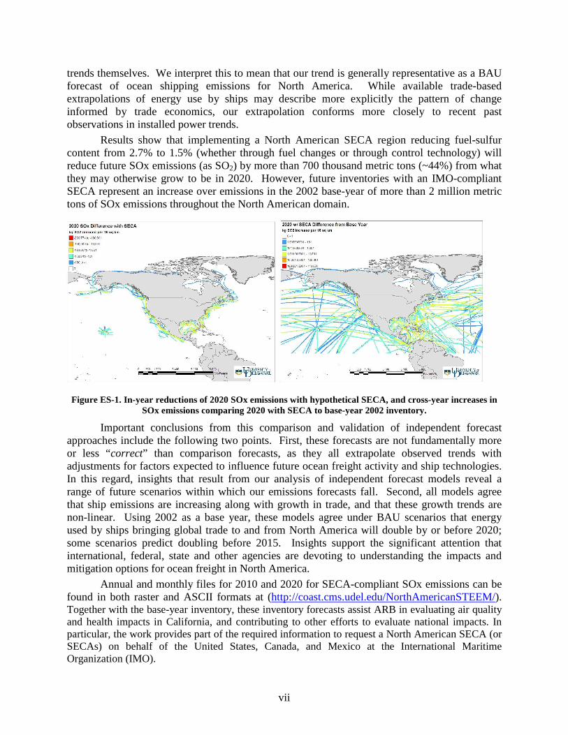
Results show that implementing a North American SECA region reducing fuel-sulfur content from 2.7% to 1.5% (whether through fuel changes or through control technology) will reduce future SOx emissions (as SO2) by more than 700 thousand metric tons (~44%) from what they may otherwise grow to be in 2020. However, future inventories with an IMO-compliant SECA represent an increase over emissions in the 2002 base-year of more than 2 million metric tons of SOx emissions throughout the North American domain.

Figure ES-1. In-year reductions of 2020 SOx emissions with hypothetical SECA, and cross-year increases in SOx emissions comparing 2020 with SECA to base-year 2002 inventory.

Important conclusions from this comparison and validation of independent forecast approaches include the following two points. First, these forecasts are not fundamentally more or less “correct” than comparison forecasts, as they all extrapolate observed trends with adjustments for factors expected to influence future ocean freight activity and ship technologies. In this regard, insights that result from our analysis of independent forecast models reveal a range of future scenarios within which our emissions forecasts fall. Second, all models agree that ship emissions are increasing along with growth in trade, and that these growth trends are non-linear. Using 2002 as a base year, these models agree under BAU scenarios that energy used by ships bringing global trade to and from North America will double by or before 2020; some scenarios predict doubling before 2015. Insights support the significant attention that international, federal, state and other agencies are devoting to understanding the impacts and mitigation options for ocean freight in North America.

Annual and monthly files for 2010 and 2020 for SECA-compliant SOx emissions can be found in both raster and ASCII formats at (http://coast.cms.udel.edu/NorthAmericanSTEEM/). Together with the base-year inventory, these inventory forecasts assist ARB in evaluating air quality and health impacts in California, and contributing to other efforts to evaluate national impacts. In particular, the work provides part of the required information to request a North American SECA (or SECAs) on behalf of the United States, Canada, and Mexico at the International Maritime Organization (IMO).

1

INTRODUCTION

This report is intended to assist the role of the California Air Resources Board (ARB) and other agencies evaluating the feasibility and extent of a North American Sulfur Emissions Control Area (SECA) as defined by the International Maritime Organization (IMO) in terms of potential impact to air quality and human health by oceangoing commercial marine vessels in transit. Using a spatially-resolved, activity-based inventory of North American shipping activity derived from 172,000 port calls in 2002 to Canada, Mexico, and the United States, we adjust the base-year inventory to estimate emissions from commercial marine vessels for 2010 and 2020. Using observed trends in installed power by cargo and passenger vessels calling on North America, we produce two classes of forecasts: 1) an unconstrained forecast applying a common growth trend to forecast a business as usual (BAU) scenario without sulfur controls; and 2) a with-SECA scenario assuming IMO-compliant reductions in fuel sulfur to 1.5% by weight for all activity within the Exclusive Economic Zone (200 nautical miles) of North American nations. This report summarizes the baseline model, presents an empirically representative growth rate based on a comparative analysis of several forecasting approaches, and discusses the implications of the inventories with and without SECA reductions.

Tasks 3 and 4 Questions & Research Objectives

A primary objective of this project is to describe a regional scale methodology for estimating commercial marine vessel (CMV) emissions in coastal waters (i.e., the Exclusive Economic Zone or EEZ) that is consistent with port-based inventory methods. Methodology for current (base-year) inventories was addressed in large part through Tasks 1 and 2, for a base year of 2002. Tasks 3 and 4 contribute to this objective by adjusting the 2002 North American inventory for future years to allow a comparison of scenarios with and without sulfur emissions control, specifically: Task 3 Forecast how baseline emissions may change in future years. Future emissions will be dependent

in part upon the changes in emission factors (due to MARPOL Annex VI, other policy, and other changes in engine characteristics), changes in vessel size and number. Additionally, changes may occur in vessel activity patterns and trade routes, and changes in fuel quality (especially sulfur content) – from a mix of technology, economic, and/or policy drivers.

Task 4 Forecast future-year ship emissions under a potential SECA designation. Modification of future-year baseline emissions are made using MARPOL Annex VI requirements that requires the sulfur content of marine fuel used by marine engines within a SECA be equal to or less than 1.5% S by weight.

This project will support ARB efforts to understand the significance of ship emissions, by providing forecasts of CMV emissions under assumptions that describe trade-driven fleet growth, technological changes, and potential designation of special areas under the IMO’s MARPOL Annex VI convention, called SOx Emission Control Areas (SECAs). We derive emissions forecast trends directly from aggregate installed power of ships calling on North American ports; this is because emissions are directly proportional to engine power and load, which for at-sea conditions is highly correlated with total installed power on commercial ships.1 To validate our power-based extrapolation assumptions, we employ a comparison of historic trends and forecast indicators related to maritime trade and energy to provide reasonable insight

1 This direct proportionality of stack emissions to engine power is implicit in the use of power-based emissions factors in activity-based inventory best practices.

2

into a range of feasible forecasts. Individually, none of these comparison forecasts can be considered more correct than another, as they represent different assumptions about the relationship between transportation energy, trade, and North American port activity. However, taken together, they reveal a bounded range of trends with common insights useful in comparing sulfur controls with no action. Our analysis confirms that power-based trends are representative at several scales (port, region, coastal, and national) and informed by historic data, producing a forecast of North American ship emissions with and without IMO-compliant sulfur reductions.

Background

Air pollutants from marine vessels account for a non-negligible portion of the emissions inventory and contribute to air quality, human health and climate change issues at local, regional and global levels (1-23). According to the U.S. EPA, heavy duty truck, rail, and water transport together account for more than 25% of U.S. CO2 emissions, about 50% of NOx emissions, and nearly 40% of PM emissions from all mobile sources (24, 25). In Europe, freight modes together generate more than 30% of the transportation sector’s CO2 emissions (26). In California, marine vessel ship emissions are a significant concern with regard to state implementation of federal air quality requirements (http://www.arb.ca.gov/msprog/offroad/marinevess/marinevess.htm), particularly for air districts (19, 27)) and for major ports (http://www.portoflosangeles.org/ and http://www.polb.com/).

Better estimation of current and future emissions inventories, including spatial representation, is needed for atmospheric scientists, pollution modelers, and policy makers to evaluate and mitigate the impacts of ship emissions on the environment and human health. In fact, understanding the nature of commercial marine (e.g., cargo) vessel activity and energy use serves both environmental and goods movement goals for the State of California and the nation. This is particularly true for major ports which represent the node connecting imported and exported ship cargoes with road and rail freight transportation serving the U.S. and global economies.

Summary of Significance

This work forecasts emissions from commercial marine vessels (CMVs) in California and across North American regions (including U.S., Canada and Mexico). Power-based growth trends were validated through comparison with other marine vessel and oceangoing forecasts at global, national, and regional scales, including major ports in California. We also compared forecasts for other freight modes, compared draft results of a trade-energy model developed for the U.S. EPA by RTI International as part of the North American SECA team activities. Our BAU results conclude that ship energy use and emissions will grow significantly through 2020, with doubling from the 2002 base year inventory before 2020. We adjust for a slightly lower growth rate for NOx due to IMO-compliant engines diffusing into the fleet through new vessel orders or major conversions of existing vessels. Spatially resolved inventories represent national average growth scenarios; power-based growth rates for selected regions are summarized (see Table 1). Data support extended work producing maps using regionally-specific growth rates; however, additional modeling is needed beyond the scope of this project (discussed in the Uncertainty and Bounding part of the Summary section).

Results of this research will support ARB efforts to develop effective measures to reduce ship emissions, and provides information needed to request a North American SECA (or several SECAs) at IMO.

3

MATERIALS AND METHODS

This section describes principles, methods, and data used to produce future emissions inventory scenarios for North America. Three critical questions for forecasting freight activity and environmental impacts include:

1. Baseline Conditions: What are freight energy and activity patterns? 2. Rates of Change: What is forecast trend in energy needed? 3. Patterns of Change: Where is future freight activity located?

While interrelated, these questions may be validated with some independence. In this

work, additional complexity involves understanding the spatial nature of the forecasted seaborne trade, energy use, and emissions. In particular, a spatially allocated baseline estimate must include identification of major trade routes, and make adjustments for routes on which the most energy-demanding vessels operate. The spatially allocated forecast would ideally consider how asymmetric growth among commodities and vessel types may affect the spatial dimensions of the forecast, and would include adjustments for emissions control measures as existing or forecasted policies begin to take effect.

We use the baseline inventory from ARB project Tasks 1 and 2 (28), partly funded by the Council on Environmental Cooperation. We derive emissions forecast trends directly from aggregate installed power of ships calling on North American ports; this is because emissions are directly proportional to engine power and load, which for at-sea conditions is highly correlated with total installed power on commercial ships.2 To validate our power-based extrapolation assumptions, we explore a range of forecasts and trends that derive from trade flows, marine energy consumption estimates, available sales statistics, and detailed scenarios about possible future fleet activity. Our analysis is pluralistic in its inclusion of forecast trends, looking for robust forecast trends rather than attempting to conform to a single likely scenario. We evaluate how power-based trends differ across North American, U.S., and West Coast regions to help illustrate expected asymmetry of faster-growing major trade routes with global average trends. This ensures that our power-based extrapolation provides a representative forecast path within the bounded range of potential trends from which to produce spatially resolved forecasts for 2010 and 2020. This helps us begin to consider how spatial representation of future ship energy and emissions in North America may differ from other sources and regions. Our emissions trends are consistent with available backcast trends in installed power and with independent forecasts for major ports. Lastly, this comparison leads us to identify remaining limitations in these spatial forecasts and future improvements to provide additional insights.

Baseline: Ship Traffic Energy and Environmental Model (STEEM) Description

By applying advanced GIS tools and using better data sets, STEEM adopts the strengths of both top-down and bottom-up approaches and attempts to overcome the weaknesses in each approach and improves ship emissions inventory both mathematically and theoretically. First, the model builds an empirical waterway network based on shipping routes revealed from observed historical ship locations. The spatial allocation is more accurate than a bottom-up approach, which uses speculative routes, and than a top-down approach, which uses biased spatial proxies.

2 This direct proportionality of stack emissions to engine power is implicit in the use of power-based emissions factors in activity-based inventory best practices.

4

Second, as in a bottom-up approach, this model estimates energy use and emissions using complete historical ship movements, ship attributes, and the distances of routes. The calculations are expected to be more accurate than a top-down approach, which relies on the statistics of the world fleet and its operating profiles. Third, the automation of repetitive processes makes this method capable of producing global energy and emissions inventories, which is a daunting task with existing bottom-up approaches. Fourth, since the network can be updated, modified, re-used, and shared among users, STEEM is perhaps more cost-effective than both the top-down and the bottom-up approaches. STEEM improves the baseline emissions inventory for North American shipping in the following ways:

1. STEEM employs an emprical global waterway network derived from 20-year International Comprehensive Ocean-Atmosphere Data Set (ICOADS) data;

2. The model estimates emissions from nearly complete historical North American shipping activities (some 172,000 trips in U.S. Foreign Commerce Entrances and Clearances data set and Lloyds’ Movement data set) and individual ship attributes while a top-down approach estimates emissions based on statistical analysis;

3. The model is constructed using advanced GIS network analyst technology to solve the most probable route for each individual trip on a global scale;

4. STEEM establishes explicit mathematical relationships among trips, ships, routes, pairs of ports, and segments of the waterway network using a matrix approach;

5. STEEM uses actual lengths of routes, together with service speed of each individual ship, to calculate hours of operation while top-down approaches estimate annual hours of operation based on fleetwide statistics;

6. STEEM follows best practice to estimate emissions based on ship installed power, service speed, and traveling distance for each trip;

7. STEEM assigns emissions based on the locations of solved routes while earlier bottom-up approaches drew straight lines between origins and destinations manually and top-down approaches allocate global emissions based on biased proxies;

8. STEEM captures transit traffic which contributes to local air quality problems in some areas like Santa Barbara, CA, while port-wide inventories have often ignored or been unable to quantify these effects.

Forecasting principles

Forecasts can differ depending on their purposes and scales. Some forecasts look to reveal where timely investment and action at a local scale or by a single firm can produce the most benefit (e.g., profit). Validity of insights is determined by whether recommended actions produce expected outcomes for a given decision, not whether the forecast trend or future value is realized. Other forests are intended to be conservative or aggressive; that is, they intend to be biased to serve the decision makers’ value and tolerance for risk and surprise. This may describe large scale forecasts such as emissions or trade trends. One challenging class of forecasts may be considered “difference” forecasts, where alternative scenarios illustrate how “a path taken” may differ from “a path not taken” rather than to determine which is most probable. These kinds of forecasts are common in policy domains, such as energy, environment, and economics (e.g., IPPC scenarios). Certainly, freight forecasting presents one challenging example, especially at the international or multinational scales, and especially when considering policy actions like a SOx Emissions Control Area (SECA) under IMO MARPOL Annex VI (29).

5

Admittedly, the quality of forecasts of maritime shipping and trade is limited (30), and thus forecasting of environmental impact from shipping is constrained by the quality of shipping and trade forecasts. Rather than attempt to define one forecast path among many conditional events determining future ship emissions, we employ a comparison of historic trends and forecast indicators related to maritime trade and energy to provide reasonable insight into a range of feasible forecasts. Individually, none of these forecasts can be considered more correct than another, as they represent different assumptions about the relationship between transportation energy, trade, and North American port activity. However, taken together, they reveal a bounded range of trends with common insights useful in comparing sulfur controls with no action. We look for converging growth trends that are representative at several scales (port, region, coastal, and national) and informed by historic data. These lead to a set of principles for describing how freight transport emissions may change:

1. Define the forecast domain broadly through multiple perspectives on freight and economy. 2. Compare global, large regional forecasts with local efforts for converging insights, perhaps

allowing for probabilistic assessment. 3. Include the rear-view mirror in forecasting (i.e., compare with persistence). 4. Consider first principles involving energy and environment: Some work-energy relationship

must hold if fuel price matters to freight. 5. Make extrapolation adjustments as simple as possible, but no simpler: Assumptions inter-

relating energy, economy, and technology should be checked for potential inconsistencies. 6. Look for surprise, avoid overconfidence: Recognize heterogeneity at all scales; use detailed

scenarios to help broaden or delineate the forecast range, but do not rely on them as likely.

Installed power as first-order trend indicator for commercial marine emissions

Given that energy used and emissions produced during goods movement increases at a rate correlated to growth in activity, a number of proxies may be used to estimate inventory growth rates. These include: economic activity (GDP and imports/exports value), trade activity (tons and ton-miles), fuel usage (sales and estimates). All of these are indirect proxies (second or higher order) of the activity that produces emissions. Except for fuel usage statistics, none directly describe power requirements for shipboard power plants (propulsion and auxiliary engine systems). Best practices for CMV emissions inventories typically use power-based (or fuel-based) emissions factors, because of the implicit proportionality between engine load and pollutant emissions – especially for uncontrolled sources (31, 32). Therefore, we derive emissions trends directly from installed power data for ships calling on North American ports.

Assumptions we must make to use trends in installed power are rather simple: 1) commercial marine vessels in cargo service generally design power systems to satisfy trade route speed and cargo payload requirements; in other words, there is no economic reason to design propulsion systems for containerships, tankers, etc., with more power than their cargo transport operation requires; 2) commercial marine vessels operate under duty cycles that are well understood, especially at sea speeds; these speeds utilize the majority of installed power as reflected in best practice methodologies for activity based inventories of energy and emissions from ships; 3) ships in commercial cargo service on major trade routes (to a major and growing market like North America) reflect the best fit of ship design to service requirements; in other words, the trends revealed in installed power of ships calling on North American ports directly reveals the trend in speed and size for these routes. With these assumptions, trends in installed power reveal the correlated trend in energy use by ships.

6

We used installed power data associated with port calls from USACE and Lloyds Registry (for U.S. activity) and from LMIU data (for Canada and Mexico). We used historic data as far back as 1997, where installed power data characteristics were provided. Where data were missing in the installed power field for some vessels, we used linear regression statistics within each vessel type associating gross registered tonnage (GRT) and rated power to fill data gaps.

Depending on change in energy intensity and/or emissions through investments in economies of scale, fuel conservation measures, or emissions control measures, the rate of change in energy and emissions could be a modified growth curve from the growth in cargo activity. If so, this should be observable directly in different rates of change for installed power on ships providing goods movement compared to changes in cargo volume. In other words, if a fleet of ships can carry more cargo without a proportional increase in installed power, then it must be adopting improved technologies (e.g., hull forms, engine combustion systems, plant efficiency designs) or innovating its cargo operations (e.g., payload utilization).

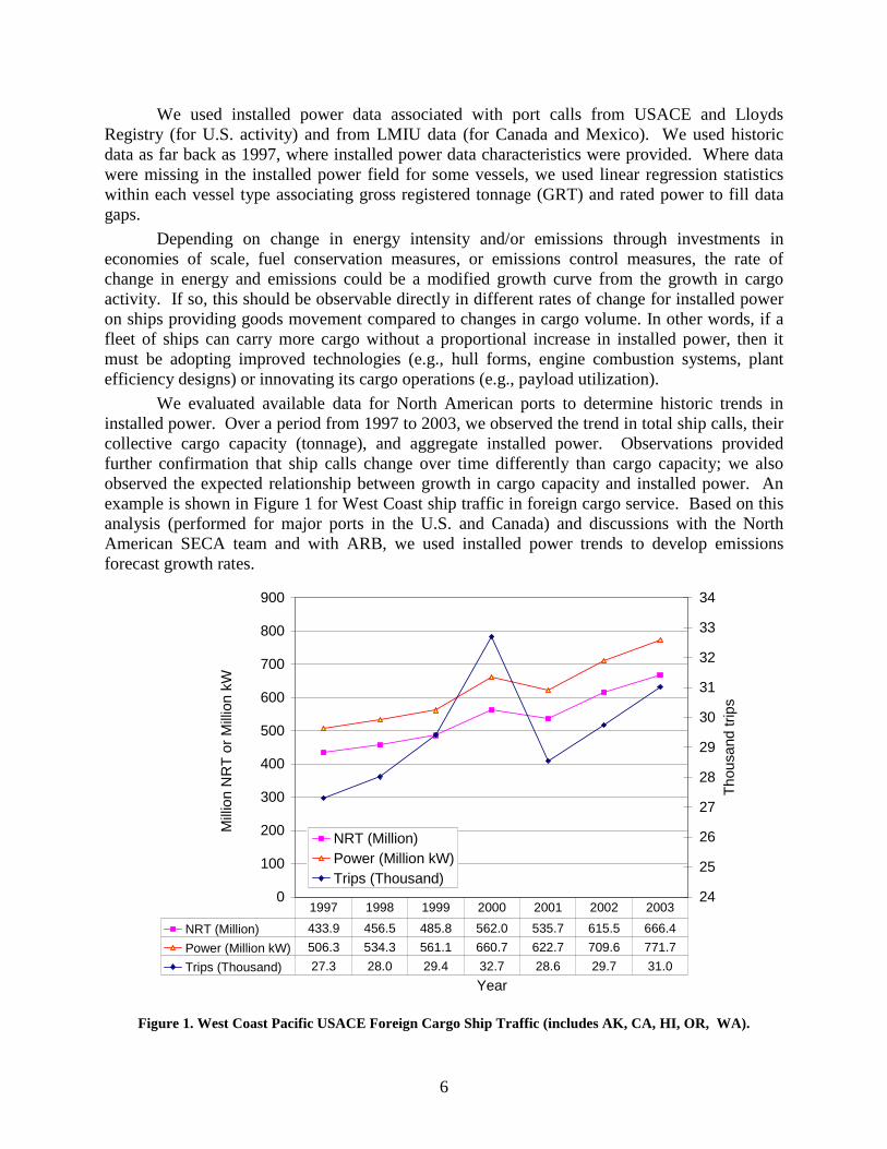
We evaluated available data for North American ports to determine historic trends in installed power. Over a period from 1997 to 2003, we observed the trend in total ship calls, their collective cargo capacity (tonnage), and aggregate installed power. Observations provided further confirmation that ship calls change over time differently than cargo capacity; we also observed the expected relationship between growth in cargo capacity and installed power. An example is shown in Figure 1 for West Coast ship traffic in foreign cargo service. Based on this analysis (performed for major ports in the U.S. and Canada) and discussions with the North American SECA team and with ARB, we used installed power trends to develop emissions forecast growth rates.

0

100

200

300

400

500

600

700

800

900

Year

Mill

ion

NR

T o

r M

illio

n kW

24

25

26

27

28

29

30

31

32

33

34

Tho

usan

d tr

ips

NRT (Million)Power (Million kW)Trips (Thousand)

NRT (Million) 433.9 456.5 485.8 562.0 535.7 615.5 666.4

Power (Million kW) 506.3 534.3 561.1 660.7 622.7 709.6 771.7

Trips (Thousand) 27.3 28.0 29.4 32.7 28.6 29.7 31.0

1997 1998 1999 2000 2001 2002 2003

Figure 1. West Coast Pacific USACE Foreign Cargo Ship Traffic (includes AK, CA, HI, OR, WA).

7

A variety of curves could be fit to the multi-year data, and fitting compound growth curves to historic data points requires some judgment. An unconstrained exponential curve fit would likely overestimate future emissions, particularly given expected shipping cycles (30). As discussed above, a linear growth rate did not match known or expected technology changes relative to cargo growth; a linear trend in energy use would imply less power required to achieve the cargo throughput – where cargo volumes are projected to see compounded growth. We don't believe that average technology in the fleet will change that much from its current path over the next 35 years without strong policy incentive or substantial changes in fleet energy pricing and supply. Overall, fleet propulsion technologies will remain more similar than different to the current profile at least through 2040. Moving more cargo will require more power, in a similar manner to the current fleet (either through larger ships, faster ships, more ships, or some combination). Moreover, we did not identify physical capacity limits to ports or shipping routes (that are not being addressed through infrastructure investment) which would constrain trade growth.

Most forecasts essentially take historic trends for some recent period and extrapolate with adjustment for expected change in trends (e.g., response to economic and population drivers affecting global trade or consumption). Shipping cycles, recessions, and other surprises are likely to produce growth trends less aggressive than simple exponential curve fits. We recognized the need for similar adjustment in our forecasts; however, we could not determine a location in time or the adjustment magnitude for these events. In other words, we expect that future trade growth may not conform to a simple growth rate assumption, but we hesitated to arbitrarily insert an “inflection point” in out-year forecasts corresponding to optimistic or pessimistic assumptions.

A simple exponential curve fit to installed power produced an initial growth rate estimate of 7.1% per year for North America, before averaging with a linear extrapolation. Through discussions with ARB, we agreed that the unconstrained exponential trend and the linear trend define bounding limits for expected change in ship activity. Averaging these curves defines an arbitrary middle-growth trend, which implicitly describes a mix of positive and negative drivers for ship energy requirements without articulating a detailed scenario of conditional events. After adjustment, we estimate a growth trend for North America (including United States, Canada, and Mexico) of about 5.9%, compounded ,

Other freight energy and emissions forecasts Freight transportation, particularly international cargo movement, is an important and

increasing contributor to global and national economic growth, as well as state and regional economic growth in and around major cargo ports. The multimodal and multicargo freight context must be considered when forecasting oceangoing environmental trends. This is because all freight modes respond to common drivers of change (e.g., economic growth, population demographics, energy prices), and cross-mode influences need to be included (e.g., metropolitan road congestion around one port diverting some cargoes to other ports). This applies whether one is considering air emissions or other environmental impacts. Convergence is emerging on global estimates – at least in terms of major insights, through academic dialogue about uncertainty ranges in oceangoing energy and emissions (33).

The U.S. Bureau of Transportation Statistics (BTS) recently released a report that describes North American freight activity and trends (34). This document reports growth rates

8

for North America above 7.4% for international trade and above 7.2% across all measures of value, and states that:

“Since 1994, the value of freight moved among the three countries has averaged almost 8 percent annual growth in both current and inflation-adjusted terms, compared with about 7-percent growth for U.S. goods trade with all countries (table 1). In 2005, both goods trade and gross domestic product (GDP) grew in inflation-adjusted terms. Except in 2001 and 2002, during the past decade, U.S. trade with Canada and Mexico has increased at a faster rate than U.S. GDP.”

Growth in goods movement by dollar value may be expected to differ from growth in the volume of goods moved, and in the change in activity by the multimodal fleets (ships, trucks, trains, and aircraft) moving cargo. This section describes growth trends for freight transportation reported by or derived from available sources that are used to consider the validity of growth trends derived for CMV inventoies.

Economic forecasting of goods movement We confirmed that the contribution of international trade is increasing as a proportion of

U.S. gross domestic product (GDP) – i.e., freight transportation is growing faster than U.S. GDP (34, 35). Economic activity related to imports and exports together contribute about 22% of recent U.S. GDP in recent years; goods movement contributed about 10% of GDP in the 1970s. Moreover, the dominance of containerized cargoes in seaborne trade suggests that truck and containerized shipments may double by 2025 or sooner (36). GDP in the U.S. is growing at ~3.7% CAGR since 1980, and the freight sector is growing at ~6.4% CAGR over the same period (35). This freight-sector growth rate in terms of dollar value is reflected in the observed ~6.3% to 7.2% annual growth rates of “high-value” containerized trade volumes, particularly from Asia (37).

Studies for Southern California (San Pedro Bay) ports agree that growth in cargo volumes equivalent to 6-7% compounding annual growth rates is expected (38-41). However, increased cargo may not produce a corresponding increase in port calls, as some studies interpret (39). Historic data on port calls to San Pedro Bay have shown the number of ship calls remained between 5,000 and 7,000 calls per year since the 1950s (42). This demonstrates that increasing cargo throughput is related to technology innovation (e.g., larger ship sizes, higher speeds, and containerization) that promotes economies of scale, more so than increased cargoes determine the number of voyages. In fact, the trend in cargo growth is more closely related to work and energy, i.e., installed power, than to ship calls.

Activity-based modeling of freight transportation

Seaborne cargo activity has increased at significant rates over time. World seaborne trade growth has increased monotonically except for a short period in the early 1980s (43-46). Containerized trade is growing faster than global rates. Figure 2 illustrates containerized cargo trends 1997-2005. U.S. Maritime Administration (MARAD) statistics include cargo on both government and non-government shipments by vessels into and out of U.S. foreign trade zones, the 50 states, District of Columbia, and Puerto Rico, excluding postal and military shipments; AAPA statistics describe total container throughput, including empty container movements. Containerized cargo throughput (including empty container movements) grew at ~6.5% CAGR since 1985, with imported cargo grow since 1997 at more than 10% CAGR and total cargo TEUs (excluding empty container movements) growing at ~7% CAGR since 1997. Given the high-

9

value nature of containerized cargoes, it is not surprising that these growth trends are most similar to growth in the value of cargo moved, reported by BTS.

0

5

10

15

20

25

30

35

40

45

1980 1985 1990 1995 2000 2005

Mill

ion

TE

Us

TEU throughput Total Cargo TEUs Export TEUs Import TEUs

Figure 2. Container statistics from U.S. Maritime Administration and American Association of Port Authorities (47, 48).

Conceptually, growth in seaborne cargo movement should influence (if not determine) activity growth in the freight modes (truck and rail) carrying imports and exports to or from U.S. metropolitan regions and inland regions. For example, if growth in rail and truck modes is primarily a result of increasing imports, observed in the U.S. to range between 4.6% and 4.8% CAGR for all cargoes and between 6% and 9% for containerized (intermodal) cargoes (~6.5% CAGR for total container throughput including empty containers), then combining these modes should reflect seaborne trade growth rates (48, 49). The multimodal transportation of empty containers presents a unique challenge in understanding how international goods movement affects landside freight modes (50). Moreover, trucking and rail movements include exported and domestic freight movements, which are growing at much lower rates than containerized imports, effectively dampening national growth rates in intermodal freight transportation compared to port throughput. Considering these activities together helps provide an intuitively consistent explanation reconciling steeper seaborne trade trends reported in major ports, and obtained or derived from economic and trade analyses, with less-steep truck and rail freight trends. In other words, we should expect growth rates in goods movement to be shared among modes because freight transportation is an intermodal network of imports, exports, empty repositioning, and domestic freight flows.3

3 This background discussion does not necessarily imply a direct relationship between energy and emission growth rates and seaborne trade growth rates; depending on efficiency gains and economies of scale (e.g., shown for the rail sector), the rate of change in energy and emissions for ships could be different. This background reinforces the purpose of and need for the forecasts analysis presented in this report.

10

The U.S. Department of Transportation launched two of the first federal efforts to consider together multimodal and intermodal freight effects of imported cargoes, generally through its “Assessment of the U.S. Marine Transportation System and spatially through the Freight Analysis Framework (FAF) (51, 52). This work produced a forecast of freight transportation activity based on trade increases, primarily to identify infrastructure needs rather than estimate energy and environmental impacts. According to the Freight Analysis Framework (52),4 domestic freight volumes will grow by more than 65 percent from 1998 levels by the year 2020, increasing from 13.5 billion tons (in 1998) to 22.5 billion tons (in 2020). This represents a ~2.3% compound annual growth rate (CAGR), similar to that obtained from VMT growth rates (not adjusted for sales growth) in MOVES (53). In other reports, truck freight has doubled since 1980 (an average annual increase of 3.7%), while domestic waterborne freight has declined by nearly 30% (an average annual decline of 1.8%) (54).5 These rates represent the lowest growth trends we could find in the literature for goods movement.

Emissions and energy forecasting of goods movement

If growth in GDP and trade volumes is compounded as forecast by economic and transportation demand studies, then growth in energy requirements should be non-linear also. Freight energy use is correlated to increases goods movement, unless substantial energy efficiency improvements are being made within a freight mode (e.g., U.S. rail) or across the logistics supply network. Even assuming that efficiency improvements from economies of scale reduce energy intensity and emissions rather than being directed to larger and faster ships (e.g., containerships), compounding increases in trade volumes outstrip energy conservation efforts unless technological or operational breakthroughs in goods movement emerge.

Proportional relationships between environmental impacts and goods movement trends are reflected in recent port and regional studies of economic activity and goods transportation, particularly those focused on Southern California ports (38, 55-57). Federal energy forecasts also link freight activity (and associated energy consumption) to economic growth projections. For example, the EIA Energy Outlook “uses projections of dollars of industrial output to estimate growth in freight truck travel; industrial output is converted to an equivalent measure of volume output using freight adjustment coefficients” that assume constant average ton-miles per truck-year (58).

Correlations between energy, emissions, and economic activity are observed also in modal emissions forecasts for freight transportation. Until recently, most state and federal studies have considered trucking forecasts to be part of an onroad domain, and other freight modes (e.g., rail and waterborne) to be nonroad, even though containerized freight flows are more typically inter-modal complements rather than multimodal substitutes. EPA’s Emissions Growth Analysis System (EGAS) contains growth factors for on-road mobile source categories, generally computing growth factors based on VMT projections (59, 60). Acknowledging that vehicle miles traveled (VMT) growth factors in EGAS are not differentiated by road classification or vehicle type, EPA suggests that other methods, like travel demand forecasting or regional growth rates may be more accurate. Since then, the EPA has been working to develop improved models specific to mobile sources (61).

4 See Freight Analysis Framework documents at http://ops.fhwa.dot.gov/freight/freight_analysis/faf/. 5 BTS Pocket Guide to Transportation 2003, http://www.bts.gov/publications/pocket_guide_to_transportation/2003/.

11

Currently, growth factors embedded in U.S. mobile source energy and emissions models appear to capture better this economic-driven growth in freight transportation. Growth factors for trucking (single-unit and combination trucks) in the U.S. EPA’s mobile source models include a combination of a population (sales) and VMT growth factors, with adjustments for fuel economy and other operational factors (53). EPA compared rail freight ton-miles with railroad distillate fuel consumption data to indicate substantial improvements in rail freight energy intensity, adjusting emissions based on regulatory requirements (62). And, in its 2003 rulemaking, EPA assumed that freight growth was linked to increased tonnage volume (21).

Historic and future growth rates for particular modes are consistent with coupled growth in economic-energy-emissions trends. For example, EPA projects that truck population and VMT will increase by 4.2% to 4.8% CAGR between 2002 and 2025 (53). For rail, EPA showed that growth rates in cargo ton-miles transported nearly doubled in recent periods, from ~2.4% CAGR between 1980 and 1995 to ~4.8% CAGR between 1990 and 1995 (illustrated in Figure 1-1 in U.S. EPA’s regulatory support document). In fact, updating observed growth rates in cargo ton-miles moved by rail to include more recent years reveal a rail-cargo growth rate of ~3.6% CAGR from 1985 to 2004 (63, 64).

For the marine sector, EPA’s 2003 forecast methodology improved the similarity between economic and emissions forecasts, although emissions forecasts represent a CAGR of about 3.4% (range of 2.8% to 3.8%, depending on pollutant). While shipping growth rates accounted for the effect of increased tonnage in a newer fleet, they do not consider the effect of faster speeds – specifically the additional installed power to meet combined size and speed requirements. Correcting for these factors brings the forecasts for international marine activity into closer agreement with trucking growth rates (especially when rail cargo volume increases are considered), and better describes the role of imports growth on the intermodal freight system.

California studies also describe significant growth expected in commercial marine emissions. The recent Clean Air Action Plan for Southern California ports estimates that emissions of NOx and PM from oceangoing vessels will increase at baseline rates between 5.5% and 6% CAGR, respectively, unless measures are taken to reduce emissions (65).6 These growth rates are consistent with trade growth rates, perhaps modified for IMO-compliant NOx reductions in new vessels expected to call on California ports and descriptive of modest improvements in fuel efficiency through fleet modernization and economies of scale.

Validation of power-based trends

We also compared our power-based trend to early results of a trade-energy model developed along with our work for the SECA team (by RTI under EPA direction). While that work is in draft form, our power-based and their trade-energy-based approaches compare well. In Figure 3, we show bounding curves (exponential and linear) and the average growth curve for Southern California ports. We converted growth trends in comparison studies from the no-net-increase study and from the RTI trade-energy model (38, 66) to describe change in installed power and plotted them in Figure 3 with our extrapolation.7 We observe good agreement at this scale between the draft RTI model and our trends. Moreover, while the no-net-increase (NNI) forecast produces nearly the same result for 2020, neither of these approaches describes the

6The Clean Air Action Plan shows emissions control measures may offset near-term growth (at least through 2011) if fully implemented (see Table 6.4). 7 NNI shows only the Southern California ports of Los Angeles and Long Beach, while the RTI work describes the “South Pacific” ports, which are considered to be mainly LA and LB but could include Oakland.

12

substantial increases estimated by the NNI report in the near-term as a result of planned investment in the port(s) (38). These independent derivations of growth trends describe at least a doubling of commercial marine energy use in California by 2020, corresponding to similar change in the expected port cargo throughput.

0

200

400

600

800

1000

1200

1990 1995 2000 2005 2010 2015 2020 2025 2030

Fo

reca

sted

Tra

nsp

ort

En

erg

y (k

W)

Unconstrained 7-point Trend

Baseline NNI

Average Unconstrained-Linear

Linear Trend

RTI US South Pacific

Figure 3. South Coast (South Pacific) growth rates derived from historic data (1997-2003), showing upper-bound (exponential), lower-bound (linear), and average trends. Also shown are trends derived from the NNI

Task Force and from the draft RTI trade-energy model.

Agreement between the draft trade-energy model by RTI and extrapolation of observed data is even stronger for containerships. As shown in Figure 4, preliminary results from the draft RTI trade-energy forecast are more aggressive than our power-based extrapolation. RTI’s trade-energy model exception to calibrate on inbound containerized cargoes (“heavy-leg” activity) may explain this (66). Note excellent agreement in RTI draft model results with observed power-trend history for containership calls to U.S. ports.

These sources of growth trends and forecasts are consistent with and validate our observed trends in installed power and support our extrapolation of power-based trends to forecast emissions under business-as-usual (BAU) conditions. Using our adjusted extrapolation to forecast growth at ~5.9%, we observe that power-based growth rates derived here are higher than growth rates for land-based freight modes, by about 1% to 2%. This comparison is expected due to the fact that trucking and rail are also engaged in domestic and intra-continental trade with Canada and Mexico that would not require commercial shipping. Moreover, our forecast rates are generally lower than dollar-value growth in North American seaborne trade, and a bit lower than growth in containerized cargo volume. Again, such comparisons are expected given the importance of bulk cargoes (liquid and dry) to North American international trade. In addition, the lower growth in power-based rates compared to cargo activity provide confirming evidence that economies of scale are improving the energy intensity and emissions intensity of international shipping – but perhaps by not more than 1% to 2% overall yet. Additional analysis by vessel type could quantify these improvements in more detail, perhaps discerning relative roles of speed, size, and operational factors (e.g., average payload utilization rate). Lastly, we observe emissions and energy use by the fastest, most powerful ships (containerships) are increasing at the fastest rates, along with demand for containerized trade.

13

0

200

400

600

800

1000

1200

1400

1600

1990 1995 2000 2005 2010 2015 2020 2025 2030

Inst

alle

d P

ow

er E

stim

ate

AverageObserved Container PowerRTI Container

Figure 4. US container growth trends from data extrapolation (1997-2003) and from draft RTI trade-energy model.

14

RESULTS

This section compares results of alternative measures of growth at multiple scales, demonstrating general similarity among power-based and other ocean shipping trends. At the global scale, we evaluate available trends in energy use and/or emissions from published literature with the seaborne cargo and trade data discussed earlier. Eyring et al estimate fuel usage and emissions over a historical period from 1950 to 2000 and forecasts for 2020 and 2050 using an activity-based approach describing a BAU scenario and a number of alternate scenarios combining different ship traffic and technology assumptions (67, 68). For these purposes, we use their BAU scenario for a diesel-only fleet.

We compare world fleet trends in installed power (derived from average power by year of build) with energy trends (Eyring work and fuel sales), with trade-based historical data (tons and ton-miles), and with (preliminary) global results from RTI’s draft trade-energy model. Activity-based energy results for similar base-years (2001 or 2002) are within close agreement (31, 67, 69, 70).8 This allows us to index trends to nearly the same value and year, to index trade-based trends similarly, and to compare these with trends in installed power, as summarized in Figure 5

0

0.5

1

1.5

2

2.5

1950 1960 1970 1980 1990 2000 2010 2020 2030

Seaborne Trade (tons) RTI Trade-energy Model (world)Seaborne Trade (ton-miles) OECD HFO Int'l SalesSeaborne Trade (trend since 1985) World Marine Fuel (Eyring, 2005)Installed Power-This work

Extrapolating trends since ~1980-85 depending on data source

Figure 5. Global trend indices for seaborne trade, ship energy/fuel demand, and installed power.

Three insights emerge from this global comparison.

1) Extrapolating past data (with adjustments) produces a range of business-as-usual trends that is bounded and reveals convergence around a set of similar trends; in other words, one cannot get “any forecast they want” out of the data. If we consider that global trade and technology drivers mutually influence future trends, then we may interpret this convergence as describing a likely forecast of global shipping activity.

2) World shipping activity and energy use are on track to double by about 2030 (~2015 if one considers seaborne trade since 1985, ~2050 if one considers Eyring’s BAU trend).

8 An exception is work by Endresen et al, that tends to adjust parameters to agree with international marine fuel sales statistics; while not considered here, their results are within uncertainty ranges described in other work (3, 33, 71).

15

Growth rates are not likely to be reduced without significant changes in freight transportation behavior and/or changes in shipboard technology.

3) Confirming earlier discussion, trends in installed power are clearly coupled with trends in trade and energy. This reinforces the analysis of installed power as a proxy for forecasting growth, not only for use in baseline inventory estimates.

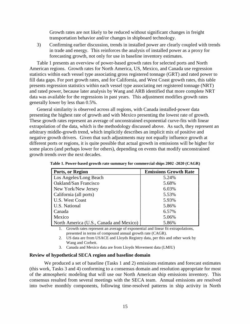
Table 1 presents an overview of power-based growth rates for selected ports and North American regions. Growth rates for North America, US, Mexico, and Canada use regression statistics within each vessel type associating gross registered tonnage (GRT) and rated power to fill data gaps. For port growth rates, and for California, and West Coast growth rates, this table presents regression statistics within each vessel type associating net registered tonnage (NRT) and rated power, because later analysis by Wang and ARB identified that more complete NRT data was available for the regressions in past years. This adjustment modifies growth rates generally lower by less than 0.5%.

General similarity is observed across all regions, with Canada installed-power data presenting the highest rate of growth and with Mexico presenting the lowest rate of growth. These growth rates represent an average of unconstrained exponential curve-fits with linear extrapolation of the data, which is the methodology discussed above. As such, they represent an arbitrary middle-growth trend, which implicitly describes an implicit mix of positive and negative growth drivers. Given that such adjustments may not equally influence growth at different ports or regions, it is quite possible that actual growth in emissions will be higher for some places (and perhaps lower for others), depending on events that modify unconstrained growth trends over the next decades.

Table 1. Power-based growth rate summary for commercial ships 2002 -2020 (CAGR)

Ports, or Region Emissions Growth Rate Los Angeles/Long Beach 5.24% Oakland/San Francisco 5.68% New York/New Jersey 6.03% California (all ports) 5.53% U.S. West Coast 5.93% U.S. National 5.86% Canada 6.57% Mexico 5.06% North America (U.S., Canada and Mexico) 5.86%

1. Growth rates represent an average of exponential and linear fit extrapolations, presented in terms of compound annual growth rate (CAGR).

2. US data are from USACE and Lloyds Registry data, per this and other work by Wang and Corbett.

3. Canada and Mexico data are from Lloyds Movement data (LMIU)

Review of hypothetical SECA region and baseline domain

We produced a set of baseline (Tasks 1 and 2) emissions estimates and forecast estimates (this work, Tasks 3 and 4) conforming to a consensus domain and resolution appropriate for most of the atmospheric modeling that will use our North American ship emissions inventory. This consensus resulted from several meetings with the SECA team. Annual emissions are resolved into twelve monthly components, following time-resolved patterns in ship activity in North

16

America, as discussed in the report for Tasks 1 and 2. The North American inventory estimates for each pollutant uses the following projection parameters from ESRI’s ArcGIS software.

Projection: Equidistant_Cylindrical Parameters: False_Easting: 0.0 – default ESRI parameter False_Northing: 0.0 – default ESRI parameter Central_Meridian: 180.0 degrees – UD defined Standard_Parallel_1: 0.0 – default ESRI parameter Linear Unit: User_Defined_Unit (1000 m) – UD defined Cell Units: kilograms per 16 square kilometers

We delivered inventory files using the following domain: left -1000 km, right 18000 km, top 8000 km, bottom 0 km.

A hypothetical SECA region conforming to the Exclusive Economic Zone (EEZ) for North America was defined for the with-SECA scenarios. Figure 6 shows the model domain and also reproduces the SOx inventory illustration for the base-year 2002. The scale shown for emissions is delineated using units common to forecast inventory illustrations discussed below.

Figure 6. Model domain showing hypothetical with-SECA region and baseline 2002 model results.

Future Emissions without SECA region (Task 3)

Based on trend comparisons discussed above, we use the following ratios for SOx forecasts: For 2010, we multiply the 2002 base year inventory by 1.61 times; for 2020, we multiply the 2002 base year inventory by 2.79 times. This corresponds to a growth rate of 5.9% compounded annually.

For NOx emissions we make adjustment for the introduction of IMO-compliant engines into the international cargo fleet. We use industry data to estimate ~11% percent average reductions in NOx for new engines complying with MARPOL Annex VI (72). Following standard assumptions for the introduction of new engines in the fleet used by ARB (and others), we estimate that about 46% of the fleet in 2010 and about 78% of the fleet in 2020 will be IMO-compliant. This accounts for fleet-weighted NOx reductions of 5% and 8.4% in 2010 and 2020, respectively, resulting in NOx multiplier ratios of 1.53 for 2010 and 2.55 for 2020.

17

Per project scope, we considered whether fuel-sulfur content may change in coming years, e.g., would refining practices result in generally higher fuel-sulfur averages over time as distillate fuels (particularly diesel) removed more sulfur. We chose not to make any adjustments to the average fuel-sulfur content in this work for two reasons. First, we observe very little change in world-average fuel-sulfur content for residual fuels over the past decade; in fact, most of the differences may be attributed to better statistical tracking on behalf of MARPOL Annex VI, more so than real changes in the global average. Second, we recognize that variation is fuel-suflur content regionally may be greater than the average change over time; we understand that EPA is sponsoring study of this issue, and that results of that work are not yet available. If such trends are proven, they can be implemented at the regional level using STEEM in future work.

An illustration of 2020 emissions without applying any SECA reductions is presented in Figure 7. Annual and monthly data files for 2010 and 2020 for all forecasted pollutants (SOx as SO2, NOx as NO2, CO2, PM, CO, and HC) are provided in both raster and ASCII formats at the project website (http://coast.cms.udel.edu/NorthAmericanSTEEM/).

Figure 7. Illustration of 2020 ship SOx emissions without SECA reductions.

Future Emissions with Potential SECA (Task 4)

To produce with-SECA forecast scenarios, uncontrolled inventories for 2010 and 2020 are modified to depict a reduction in average fuel-sulfur content from 2.7% to 1.5%, a SOx emissions reduction of about 44%. Only SOx emissions are assumed to change under this SECA scenario; no additional reductions in primary PM, NOx or other pollutants are calculated. Within GIS, we select the emissions within the hypothetical SECA region and multiply them by 66% (1 minus 44%). Similar to the forecast without SECA, this makes no assumptions for changes in fuel quality or supply between now and 2020. Such changes could occur through regulatory action in addition to an IMO-compliant SECA, or through a combination of fuel supply and price effects not considered in this work. Such considerations could be included in updated forecasts,

18

based on insights from further (ongoing) studies. Figure 8 illustrates annual SOx emissions in 2020 depicting compliance with the hypothetical SECA domain.

An illustration of 2020 emissions with SECA reductions is presented in Figure 8. Annual and monthly files for 2010 and 2020 for SECA-compliant SOx emissions can be found in both raster and ASCII formats at (http://coast.cms.udel.edu/NorthAmericanSTEEM/).

Figure 8. Illustration of 2020 ship SOx emissions with hypothetical SECA region.

It is worth noting that sulfur inventories represent stack emissions of gaseous sulfur dioxide (SO2), not aerosol sulfate. Ours is a stack emissions inventory, before total fate and transport impacts. It is inappropriate to pre-process gaseous emissions from the stack within an inventory using some set of assumptions to estimate total PM (primary plus secondary). Atmospheric modeling will convert the SO2 gas emissions to sulfate particles needed to estimate total PM health effects.

19

SUMMARY AND CONCLUSIONS

Implementing a North American SECA region reducing fuel-sulfur content from 2.7% to 1.5% (whether through fuel changes or through control technology) will reduce future SOx emissions by more than 700 thousand metric tons (~44%) from what they may otherwise grow to be in 2020 (see Figure 9).

Important conclusions from this comparison and validation of independent forecast approaches include the following two points. First, these forecasts are not fundamentally more or less “correct” than comparison forecasts, as they all extrapolate observed trends with adjustments for factors expected to influence future ocean freight activity and ship technologies. In this regard, insights that result from our analysis of independent forecast models reveal a range of future scenarios within which our emissions forecasts fall. Second, all models agree that ship emissions are increasing along with growth in trade, and that these growth trends are non-linear. Using 2002 as a base year, these models agree under BAU scenarios that energy used by ships in global trade will double by or before 2020; some scenarios predict doubling before 2015. Insights support the significant attention that international, federal, state and other agencies are devoting to understanding the impacts and mitigation options for ocean freight in North America.

Figure 9. Forecast reduction in 2020 of annual SOx emissions due to hypothetical SECA.

Figure 10 illustrates the change in SOx forecast for 2020 as a ratio of 2002 base-year emissions and in metric tons difference. Note that Figure 10 depicts only increased ship SOx emissions. Forecasted increases in trade will overcome IMO-compliant reductions in ship SOx

20

emissions in less than two decades (before 2020 at 5.9% CAGR). Specifically, our results forecast more than 2 million metric tons of SOx additional emissions throughout the North American domain, even with an IMO-compliant SECA in 2020. Similar results occur under RTI draft forecasts (at 3.7% CAGR), which under 1.5% sulfur limits will equal base-year emissions in about 2030.

Figure 11 illustrates this further by representing the change in emissions within the EEZ (hypothetical SECA) over time. This helps reveal two insights:

1. There are benefits from an IMO-compliant (1.5% fuel-sulfur SECA) over BAU trends; and

2. Health effects and/or other impacts that may be offset from the 2002 base year by implementing a SECA will return to 2002 levels within one or two decades. (Of course, mitigation benefits will be determined in other work by ARB and the SECA team.)

These insights appear robust, regardless of the range in possible forecasts. Using the forecast trend derived in this work, trade growth offsets emissions under a 1.5% fuel-sulfur SECA by 2012; using lower growth rates from preliminary RTI results, emissions within a North American SECA return to 2002 levels by 2019.

However, Figure 11 also shows that a 0.5% fuel-sulfur limit – such as has been discussed for Europe – provides substantial benefits longer into the future under reasonable growth assumptions. A North American SECA requiring 0.5% fuel-sulfur or control technologies achieving these reductions would offset trade growth continuing to the early 2030s under a 5.9% CAGR or to about 2050 under a 3.7% CAGR, respectively. This conclusion from either growth curve means that long-term emissions reductions are possible from ships operating in North American waters, and that the IMO-compliant SECA requirements (1.5% fuel-sulfur) represents an important first step.

Figure 10. Forecast increases from base-year 2002 inventory in SOx emitted in 2020 with SECA.

Uncertainty and Bounding

There are six types of uncertainty that affect these results. Two primary sources of uncertainty involving parameters directly used in this study include a) uncertainty in the base-year estimates, and b) uncertainty in the trend used to produce the forecasted inventories. Additionally, uncertainty arises from factors not addressed in this work to date – but that could improve future efforts using these methods. Additional detail could be incorporated to describe

21

better underlying drivers of change in freight activity and consumption, to include planned or proposed signals (e.g., policy action) modifying vessel activity and propulsion technology, to make alternate assumptions about fleet response in terms of under- or over-compliance with standards or in terms of price-effects, and to better depict spatially the asymmetric growth among vessel types and trade routes expected within the shipping network.

-

500,000

1,000,000

1,500,000

2,000,000

2,500,000

2000 2005 2010 2015 2020 2025 2030

Met

ric

To

ns

SO

2 in

SE

CA

5.9% Growth (This work) Preliminary RTI Growth (~3.6%)Our Trend With SECA RTI with SECA2002 Baseline 0.5% SECA at 5.9% Growth

Figure 11. Comparison of trends with and without IMO-compliant SECA, and with 0.5% SECA

Base-Year Uncertainty

The baseline inventory effort followed general best practices for calculating emissions inventories, which enables general analysis of uncertainty due to estimating input parameters, as discussed in the report for Tasks 1 and 2, and elsewhere (28, 73). Results show good agreement with other inventories, including the draft trade-energy model estimate for 2001 by RTI (66). National level uncertainty includes four major elements: A) Uncertainty in input parameter assumptions (e.g., emissions factors, engine activity profile, etc.); B) Uncertainty in U.S. domestic shipping not included in foreign commerce vessel movement data; C) Uncertainty in U.S. Army Corp of Engineers data, and in Canadian and Mexican LMIU data; and D) Spatial uncertainty in routing choices, particularly within confined bay and port regions and seasonally for open ocean routes where weather routing may occur. An uncertainty analysis was performed on fundamental input parameters in the model, and potential undercounting of voyages or their misassignment in the routing model was discussed, including opportunities to improve the baseline inventory produced by STEEM for this work.

22

Uncertainty in Trend Extrapolation

These forecasts must be considered to represent what other forecast scenarios often refer to as “business as usual” (BAU). The primary uncertainty in the forecast trend applied to the 2002 baseline inventory can be best understood in terms of backcast validation efforts described above. Improving confidence in extrapolated trends requires longer historic trends, regionally resolved. Improving the nature of extrapolations would require better articulated relationships among drivers and industry trends. However, as shown above, the extrapolated trends developed in this work are within bounded agreement with other forecasts more dependent on trade economics.

A secondary element in trend uncertainty could reside in missing data fields associating installed power with ships calling on North America. For this work, we used linear regressions within each vessel type associating gross registered tonnage (GRT) and installed power to fill data gaps. During later review, we compared overall power-based growth trends using net registered tonnage (NRT) regressions. There was less than 0.6% difference between the regressed power and reported power in registry data for 2002, indicating that both GRT and NRT regressions yield similar results. However, as we move back in time, we note empty fields in the GRT data increase faster than empty fields in the NRT data; this could result in different trend estimates for the same historic ship calls. Upon review, we confirmed that using NRT correlations with installed power could increase the 1997 estimates by less than 9%; none of the other years’ installed power totals changed much. This could decrease the overall growth trends used in this work by less than 1%.

We think this uncertainty in trend extrapolation could be worth further research, but acknowledge that revised trends would still compare well in our validation analysis. No major insights or conclusions would change. Ship emissions activity would still be on track to double before 2020 in North America, and an IMO-compliant SECA would still return to 2002 levels within two decades. A lower growth rate in installed power could indicate slightly greater reductions in energy intensity (e.g., faster decoupling of trade and emissions) over time, but this would still be within the 1% to 2% range reported in this work.

Incorporation of additional detail among drivers affecting change

Underlying drivers of freight activity and the energy systems that produce emissions will continue to merit analysis. For example, growing GDP may remain highly correlated with growth in imports as it has over past decades. This correlation could become stronger in the future, or one might consider how and whether change in population age and demographics could reduce the rate of consumption and trade in North America without a downturn in GDP. These sorts of effects on global and regional shipping are not considered in this work, either directly or through any of the BAU forecast trends considered; a potential exception could be include work by Eyring et al., which modifies growth on major trade routes greater than recent trends and North American analyses would suggest (68). Better consideration of drivers for change in freight transportation represents a rich area for future research, particularly in terms of goods movement.

Incorporation of planned or proposed signals to modify technological change trends

This work explicitly accounts for the expected impacts of NOx emissions limits imposed by MARPOL Annex VI – already in force, as discussed above. In addition to the Annex VI NOx limits, one could consider including fuel switching measures proposed by the State of California

23

for auxiliary engines and/or in a recent proposal by INTERTANKO (74). We forecast emissions without considering such interventions, to compare BAU results with a SECA regime. This enables atmospheric modeling analyses by members of the North American SECA team to consider what reductions may achieve air quality goals in North America. Future work could consider actions (e.g., emissions trading regimes) that could accelerate or out-perform a SECA for North America; recent work has begun to consider these issues (75).

Inclusion of fleet action in response to potential action

Few assumptions about influences of EU regulatory activity, IMO decisions, or changes in marine fuel supply and demand are imposed in forecasts presented here. Moreover, this work assumes full compliance with SECA requirements and no change in fleet logistics associated with these scenarios. Additional modeling of fleet responses to policy or economic signals may reveal motivations for unintended behavior and assess their likelihood. This could help clarify whether increased regulation could deter trade, or whether observations confirming such behavior are mostly anecdotal.

Spatial Limitations and Opportunities for Improvement

Overall the inventories produced for this project using STEEM are shown to be valid geospatial depictions of emissions from commercial ship activity in North America. Some limitations reveal potential for future analyses to become more accurate and descriptive. In particular, we emphasize that this work increased emissions proportionally for all routes on all North American coastlines. This necessarily underestimates growth on the West Coast where emissions from containerized trade are growing faster than the national average and overestimates emissions growth in regions where overall trade growth is slower, such as the Gulf of Mexico served mostly be bulk ships. Consideration of heterogeneous forecast trends separately for different vessel types and trade routes would produce spatial results revealing asymmetry among future trends for liner trades and bulk trades. As such, this work represents a first-order set of spatial forecasts appropriate to consider the value of a SECA for North America but not explicit enough without additional work to apply to other large-scale issues such as port development or regional shifts in traffic.

24

REFERENCES 1. Corbett, J.J. and P.S. Fischbeck, Emissions from Ships. Science, 1997. 278(5339): p. 823-

824. 2. Corbett, J.J. and H.W. Koehler, Updated Emissions from Ocean Shipping. Journal of

Geophysical Research, 2003. 108(D20): p. 4650. 3. Endresen, Ø., et al., Emission from International Sea Transportation and Environmental

Impact. Journal of Geophysical Research, 2003. 108(D17): p. 4560. 4. Endresen, O., et al., Improved modelling of ship SO2 emissions--a fuel-based approach.

Atmospheric Environment, 2005. 39(20): p. 3621-3628. 5. Streets, D.G., G.R. Carmichael, and R.L. Arndt, Sulfur Dioxide Emissions and Sulfur

Deposition from International Shipping in Asian Waters. Atmospheric Environment, 1997. 31(10): p. 1573-1582.

6. Streets, D.G., S.K. Guttikunda, and G.R. Carmichael, The Growing Contribution of Sulfur Emissions from Ships in Asian Waters 1988-1995. Atmospheric Environment, 2000. 24(26): p. 4425-4439.

7. Corbett, J.J., Emissions from Ships in the Northwestern United States. Environmental Science & Technology, 2002. 36(6): p. 1299-1306.

8. Corbett, J.J. and P.S. Fischbeck, Emissions from Waterborne Commerce Vessels in United States Continental and Inland Waterways. Environmental Science and Technology, 2000. 34(15): p. 3254-3260.

9. Corbett, J.J., P.S. Fischbeck, and S.N. Pandis, Global Nitrogen and Sulfur Emissions Inventories for Oceangoing Ships. Journal of Geophysical Research, 1999. 104(D3): p. 3457-3470.

10. Capaldo, K.P., et al., Effects of Ship Emissions on Sulphur Cycling and Radiative Climate Forcing Over the Ocean. Nature, 1999. 400: p. 743-746.

11. Lawrence, M. and P. Crutzen, Influence of NOx Emissions from Ships on Tropospheric Photochemistry and Climate. Nature, 1999. 402(6758): p. 167-170.

12. International Maritime Organization, Report on the outcome of the IMO Study on Greenhouse Gas Emissions from Ships. MEPC 45/8, 2000.

13. International Maritime Organization. Designation of the North Sea area as a SOx Emission Control Area. in MEPC 44/11/4. 1999.

14. Jonson, J.E., L. Tarrason, and J. Bartnicki, Effects of international shipping on European pollution levels. 2000, The Norwegian Metrorological Institute.

15. Commission of the European Communities and Entec UK Limited, Quantification of Emissions from Ships Associated with Ship Movements between Ports in the European Community. 2002, European Commission.

16. Isakson, J., T.A. Persson, and E. Selin Lindgren, Identification and assessment of ship emissions and their effects in the harbour of Goteborg, Sweden. Atmospheric Environment, 2001. 35(21): p. 3659-3666.

17. Kesgin, U. and N. Vardar, A study on exhaust gas emissions from ships in Turkish Straits. Atmospheric Environment, 2001. 35(10): p. 1863-1870.

18. Bailey, D. and G. Solomon, Pollution prevention at ports: clearing the air. Environmental Impact Assessment Review, 2004. 24(7-8): p. 749-774.

19. Murphy, T.M., et al. The Need to Reduce Marine Shipping Emissions: A Santa Barbara County Case Study. in Air & Waste Management Association Conference. 2003.

25

20. CONCAWE, The contribution of sulphur dioxide emissions from ships to coastal deposition and air quality in the channel and the southern north sea area. 1994: Brussels.

21. U.S. Environmental Protection Agency, Final Regulatory Support Document: Control of Emissions from New Marine Compression-Ignition Engines at or Above 30 Liters per Cylinder. 2003.

22. Lloyd's Register, Marine Exhaust Emissions Quantification Study - Mediterranean Sea. 1999.

23. Lloyd's Register and International Maritime Organization, Marine Exhaust Emission Quantification Study - Baltic Sea, in MEPC 45/INF.7. 1998.

24. Environmental Protection Agency, Inventory of U.S. Greenhouse Gas Emissions and Sinks: 1990-2003. 2005, U.S. Environmental Protection Agency: Washington, DC. p. 432.

25. Environmental Protection Agency, National Air Pollutant Emission Trends, 1970-2002. 2005, U.S. Environmental Protection Agency: Washington, DC.

26. Bates, J., et al., Economic Evaluation of Emissions Reductions in the Transport Sector of the EU: Bottom-up Analysis, UPDATED, Final Report. 2001, AEA Technology Environment: Abingdon, UK.

27. California Air Resources Board, Proposed 2003 State and Federal Strategy for California SIP. 2003, California Environmental Protection Agency: Sacramento, CA. p. 157.

28. Corbett, J.J., C. Wang, and J. Firestone, Estimation, Validation, And Forecasts Of Regional Commercial Marine Vessel Inventories, Tasks 1 And 2: Baseline Inventory And Ports Comparison, Final Report. 2006, State of California Air Resources Board and Commission for Environmental Cooperation in North America: Sacramento, CA, and Montreal, Quebec. p. 42.

29. International Maritime Organization, Annex VI of MARPOL 73/78 and NOx Technical Code. IMO-664E ed. 1998, London, UK: International Maritime Organization. 150.

30. Stopford, M., Maritime Economics. Second ed. 1997, London, UK: Routledge, Taylor and Francis Group. 562.

31. Corbett, J.J. and H.W. Koehler, Updated Emissions from Ocean Shipping. Journal of Geophysical Research - Atmospheres, 2003. 108(D20): p. 4650-4666.

32. ICF Consulting, Best Practices in Preparing Port Emission Inventories: Draft for Review, I.C. Louis Browning and E.P.S.L. Kathleen Bailey, Editors. 2005, Prepared for Office of Policy, Economics and Innovation, United States Environmental Protection Agency: Fairfax, Virginia. p. 39.

33. Corbett, J.J., Environmental Impacts of Ocean Shipping in a Freight Context: A Summary of Current Assessments, Future Trends, and Approaches to Mitigation, Draft, Working Group on Transport, Editor. 2006, Organisation for Economic Cooperation and Development (OECD): Paris, France.

34. U.S. Department of Transportation, Research and Innovative Technology Administration, and Bureau of Transportation Statistics, North American Freight Transportation. 2006, Bureau of Transportation Statistics: Washington, DC: 2006.

35. Bureau of Economic Analysis, Table 1.1.6. Real Gross Domestic Product, Chained Dollars, in National Income and Product Accounts Tables. 2006, U.S. Department of Commerce: Washington, DC. p. Today is: 11/3/2006 Last Revised on October 27, 2006 Next Release Date November 29, 2006.

26

36. TRB Executive Committee, G. Giuliano, and S. Godwin, Critical Issues in Transportation. 2006, Transportation Research Board: Washington, DC. p. 12.

37. Vickerman, J., North American Marine Trade and Transportation Trends, in Transystems Industry Presentations. 2006: Kansas City, MO.

38. NNI Task Force, Report to Mayor Hahn and Councilwoman Hahn by the No Net Increase Task Force. 2005, Port of Los Angeles: Los Angeles, CA. p. 603.

39. Mercator Transport Group, Herbert Engineering Corporation, and MDS Transmodal Ltd, Forecast of Container Vessel Specifications and Port Calls Within San Pedro Bay: Final Report. 2005, Cunningham Report: Bellevue, WA. p. 139.

40. Meyer Mohaddes Associates Inc., Port of Los Angeles Baseline Transport Study. 2004, Port of Los Angeles: Los Angeles. p. 70.

41. Parsons Transportation Group, San Pedro Bay Ports Rail Market Study, TM-1b, Draft Report. 2004, Port of Los Angeles: Los Angeles. p. 30.

42. Port of Los Angeles, et al., Control of Ship Emission in the South Coast Air Basin: Assessment of the Proposed Federal Implementation Plan Ship Fee Emission Fee Program. 1994, Port of Los Angeles: Los Angeles, CA.

43. UNCTAD, Review of Maritime Transport 2003. 2003, United Nations: Geneva. p. 158. 44. UNCTAD, Review of Maritime Transport 2002. 2002, United Nations: Geneva. p. 145. 45. UNCTAD, Review of Maritime Transport 1994. 1995, United Nations: New York and

Geneva. 46. UNCTAD, Review of Maritime Transport 2006. 2006, United Nations: Geneva. p. 160. 47. MARAD, Website pages. 2006, U.S. Maritime Administration, Department of

Transportation: Washington, DC. 48. American Association of Port Authorities (AAPA), U.S./Canada Container Traffic in

TEUs 1980-2005. 2006, AAPA: Alexandria, VA. p. spreadsheet sent from MARAD and similar found on website.

49. US Army Corps of Engineers, Waterborne Commerce of the United States: Part 5 – National Summaries. 2005, U.S. Army Corps of Engineers: Alexandria, Virginia. p. 100.

50. Le Dam Hanh, P.I., The Logistics of Empty Cargo Containers in the Southern California Region: Are Current International Logistics Practices a Barrier to Rationalizing the Regional Movement of Empty Containers? 2003, METRANS Transportation Center, University of Southern California, and California State University, Long Beach: Long Beach, CA. p. 40.

51. Slater, R. and MTS Task Force, An Assessment of the U.S. Marine Transportation System: A Report to Congress. 1999, Washington, DC: U.S. Department of Transportation. 104.

52. Federal Highway Administration and B. Lambert, Freight Analysis Framework Overview. 2002, Federal Highway Administration: Washington, DC. p. 2.

53. U.S. Environmental Protection Agency, et al., MOVES2004 Highway Vehicle Population and Activity Data, Draft. 2004, U.S. Environmental Protection Agency: Washington, DC. p. 99.

54. Bureau of Transportation Statistics, Pocket Guide to Transportation. 2004, Bureau of Transportation Statistics: Washington, DC. p. 52.

55. California Air Resources Board, Goods Movement and Ports. 2006, California Air Resources Board: Sacramento, CA.

27

56. Southern California Association of Governments, Goods Movement. 2006, Southern California Association of Governments: Los Angeles, CA.

57. Port of Los Angeles, Goods Movement Projects. 2006. 58. Energy Information Administration, Annual Energy Outlook 2003 With Projections to

2025. 2003, Department of Energy: Washington, DC. 59. E.H. Pechan & Associates Inc., Economic Growth Analysis System: Version 4.0 User's

Guide, Final Draft, G. Stella, Editor. 2001, U.S. Environmental Protection Agency: Research Triangle Park, NC. p. 84.

60. E.H. Pechan & Associates Inc., Economic Growth Analysis System: Version 4.0 Reference Manual, Final Draft, G. Stella, Editor. 2001, U.S. Environmental Protection Agency: Washington, DC. p. 82.

61. Chappell, L., Improving EPA Emissions Forecasting For Regulatory Impact Analyses, Draft. 2006, U.S. Environmental Protection Agency: Research Triangle Park, NC.

62. U.S. Environmental Protection Agency, Locomotive Emissions Standards Regulatory Support Document. 1998, U.S. Environmental Protection Agency: Washington, DC. p. 127.

63. Dennis, S.M., Improved Estimates of Ton-Miles. Journal of Transportation and Statistics, 2005. 8(1).

64. Davis, S., Transportation Energy Data Book: Edition 23. 2003, Oak Ridge National Laboratory: Oak Ridge, TN.

65. Port of Los Angeles (POLA) and Port of Long Beach (POLB), San Pedro Bay Ports Clean Air Action Plan Technical Report: Final. 2006, Port of Los Angeles (POLA) and Port of Long Beach (POLB): Los Angeles and Long Beach, CA. p. 262.

66. RTI International, et al., Unpublished Results. 67. Eyring, V., et al., Emissions from international shipping: 1. The last 50 years. Journal of

Geophysical Research - Atmospheres, 2005. 110(D17): p. D17305. 68. Eyring, V., et al., Emissions from international shipping: 2. Impact of future technologies

on scenarios until 2050. Journal of Geophysical Research - Atmospheres, 2005. 110(D17): p. D17306.

69. Corbett, J.J. and H.W. Koehler, Considering Alternative Input Parameters In An Activity-Based Ship Fuel Consumption And Emissions Model. Journal of Geophysical Research - Atmospheres, 2004. 109(D23303): p. 8.

70. RTI International, EnSys Energy & Systems Inc., and Navigistics Consulting, Global Trade and Fuels Assessment - Future Trends and Effects of Designating Requiring Clean Fuels in the Marine Sector: Task Order No. 1: Draft Report, B. Garelick and R. Smith, Editors. 2006, U.S. Environmental Protection Agency: Washington, DC. p. 72.

71. Endresen, Ø., et al., Substantiation of a Lower Estimate for the Bunker Inventory: Comment on ‘‘Updated emissions from ocean shipping’’ by James J. Corbett and Horst W. Koehler. Journal of Geophysical Research - Atmospheres, 2004. 109(D23302).

72. Wartsila NSD and K. Heim, Forward look at future emissions control measures for Sulzer RTA engines, in Marine News. 2001, Wartsila NSD: Helsinki, Finland. p. 4.

73. Wang, C., J.J. Corbett, and J. Firestone, Modeling Energy Use and Emissions from North American Shipping: an Application of Ship Traffic, Energy and Environment Model. Environmental Science & Technology, 2006. under review.

28

74. Intertanko, Revisions of MARPOL Annex VI, the NOx Technical Code and Relevant Guidelines, in Intersessional Meeting of the BLG-WGAP, BLG Working Group on Air Pollution. 2006, International Maritime Organization: London, UK.

75. Wang, C., J.J. Corbett, and J.J. Winebrake, Reducing Sulfur Emissions from Ships. 2006. in preparation .

29

LIST OF ACRONYMS AAPA American Association of Port Authorities ARB California Air Resources Board BAU Business as usual BTS U.S. Bureau of Transportation Statistics CAGR Compound annual growth rate CEC Commission for Environmental Cooperation in North America CMV Commercial Marine Vessel CO2 Carbon dioxide EEZ Exclusive Economic Zones EGAS Emissions Growth Analysis System EIA Energy Information Administration FAF Freight Analysis Framework GDP Gross Domestic Product GRT Gross Registered Tonnage IMO International Maritime Organization ICOADS International Comprehensive Ocean-Atmosphere Data Set INTERTANKO Independent Tanker Owners And Operators kW Kilowatts MARAD U.S. Maritime Administration MARPOL Maritime Pollution Convention MOVES U.S. EPA Mobile Vehicle Emissions Simulator NNI No net increase NRT Net Register Tonnage NOx Oxides of nitrogen POLA Port of Los Angeles PM Particulate matter RTI Research Triangle Institute, Inc. SECA SOx Emission Control Area SOx Oxides of sulfur STEEM Waterway Network Ship Traffic, Energy and Environment Model USACE U.S. Army Corps Engineers U.S. EPA United States Environmental Protection Agency VMT Vehicle miles traveled