Estimation Using the Generalised Weight Share...

Survey Methodology, December 2001 155 Vol. 27, No. 2, pp. 155169 Statistics Canada, Catalogue No. 12001

Estimation Using the Generalised Weight Share Method: The Case of Record Linkage

Pierre Lavallée and Pierre Caron 1

Abstract More and more, databases are combined using record linkage methods to increase the amount of available information. When there is no unique identifier to perform the matching, a probabilistic linkage is used. A record on the first file is linked to a record on the second file with a certain probability, and then a decision is made on whether this link is a true link or not. This process usually requires a certain amount of manual resolution that is costly in terms of time and employees. Also, this process often leads to a complex linkage. That is, the linkage between the two databases is not necessarily onetoone, but can rather be manytoone, onetomany, or manytomany. Two databases combined using record linkage can be seen as two populations linked together. We consider in this paper the problem of producing estimates for one of the populations (the target population) using a sample selected from the other one. We assume that the two populations have been linked together using probabilistic record linkage. To solve the estimation problem issued from a complex linkage between the population where the sample is selected and the target population, Lavallée (1995) suggested the use of the Generalised Weight Share Method (GWSM). This method is an extension of the Weight Share Method presented by Ernst (1989) in the context of longitudinal household surveys. The paper will first provide a brief overview of record linkage. Secondly, the GWSM will be described. Thirdly, the GWSM will be adapted to provide three different approaches that take into account linkage weights issued from record linkage. These approaches will be: (1) use all nonzero links with their respective linkage weights; (2) use all nonzero links above a given threshold; and (3) choose the links randomly using Bernoulli trials. For each of the approaches, an unbiased estimator of a total will be presented together with a variance formula. Finally, some simulation results that compare the three proposed approaches to the Classical Approach (where the GWSM is used based on links established through a decision rule) will be presented.

1. Pierre Lavallée and Pierre Caron, Statistics Canada, Business Survey Methods Division, Ottawa, Ontario, K1A 0T6. Email: [email protected] and [email protected].

KeyWords: Generalised weight share method; Record linkage; Estimation; Clusters.

1. Introduction

To augment the amount of available information, data from different sources are increasingly being combined. These databases are often combined using record linkage methods. When the files involved have a unique identifier that can be used, the linkage is done directly using the iden tifier as a matching key. When there is no unique identifier, a probabilistic linkage is used. In that case, a record on the first file is linked to a record on the second file with a certain probability, and then a decision is made on whether this link is a true link or not. Note that this process usually requires a certain amount of manual resolution that is costly in terms of time and employees.

We consider the production of an estimate of a total (or a mean) of one target clustered population when using a sample selected from another population linked to the first population. We assume that the two populations have been linked together using probabilistic record linkage. Note that this type of linkage often leads to a complex linkage between the two populations. That is, the linkage between the units of each of the two populations is not necessarily onetoone, but can rather be manytoone, onetomany, or manytomany.

To solve the estimation problem caused by a complex linkage between the population where the sample is selected and the target population, Lavallée (1995) suggested the use of the Generalised Weight Share Method (GWSM). This method is an extension of the Weight Share Method presented by Ernst (1989). Although this last method has been developed in the context of longitudinal household surveys, it was shown that the Weight Share Method can be generalised to situations where a target population of clusters is sampled through the use of a frame which refers to a different population, but somehow linked to the first one.

The problem that is considered in this paper is to estimate the total of a characteristic of a target population that is naturally divided into clusters. Assuming that the sample is obtained by the selection of units within clusters, if at least one unit of a cluster is selected, then the whole cluster is interviewed. This usually leads to cost reductions as well as the possibility of producing estimates on the characteristics of both the clusters and the units.

In the present paper, we will try to answer the following questions:

a) Can we use the GWSM to handle the estimation problem related to populations linked together through record linkage?

mailto:[email protected]

156 Lavallée and Caron: Estimation Using the Generalized Weight Share Method: The Case of Record Linkage

Statistics Canada, Catalogue No. 12001

b) Can we adapt the GWSM to take into account the linkage weights issued from record linkage?

c) Can GWSM help in reducing the manual resolution required by record linkage?

d) If there is more than one approach to use the GWSM, is there a “better” approach?

It will be seen that the answer is clearly yes to (a) and (b). However, for question (c), it will be shown that there is a price to pay in terms of an increase to the sample size, and therefore to the collection costs. For question (d), although there is no definite answer, some approaches seem to generally be more appropriate.

The paper will first provide a brief overview of record linkage. Secondly, the GWSM will be described. Thirdly, the GWSM will be adapted to provide three different approaches that take into account linkage weights issued from record linkage. These approaches will be: (1) use all nonzero links with their respective linkage weights; (2) use all nonzero links above a given threshold; and (3) choose the links randomly using Bernoulli trials. For each of the approaches, an unbiased estimator of a total will be presented together with a variance formula. Finally, some simulation results that compare the three proposed approaches to the Classical Approach (where the GWSM is used based on links established through a decision rule) will be presented.

2. Record Linkage

The concepts of record linkage were introduced by Newcome, Kennedy, Axford and James (1959) and for malised in the mathematical model of Fellegi and Sunter (1969). As described by Bartlett, Krewski, Wang and Zielinski (1993), record linkage is the process of bringing together two or more separately recorded pieces of infor mation pertaining to the same unit (individual or business). Record linkage is sometimes also called exact matching, in contrast to statistical matching. This last process attempts to link files that have few units in common (see Budd and Radner 1969, Budd 1971, Okner 1972, and Singh, Mantel, Kinack and Rowe 1993). With statistical matching, linkages are based on similar characteristics rather than unique identifying information. In the present paper, we will restrict ourselves to the context of record linkage. However, the developed theory could also be used for statistical matching.

Suppose that we have two files A and B containing characteristics relating to two populations A U and , B U respectively. The two populations are somehow related to each other. They can represent, for example, exactly the same population, where each of the files contains a different set of characteristics of the units of that population. They can also represent different populations, but with some natural links between them. For example, one population can be one of parents, and the other population one of

children belonging to the parents. Note that the children usually live in households that can be viewed as clusters. Another example is one of an agricultural survey where the first population is a list of farms as determined by the Canadian Census of Agriculture and the second population is a list of taxation records from the Canadian Customs and Revenue Agency (CCRA). In the first population, each farm is identified by a unique identifier called the FarmID and some additional variables such as the name and address of the operators that are collected through the Census questionnaire. The second population consists of taxation records of individuals who have declared some form of agricultural income. These individuals live in households. The unique identifier on those records is either a social insurance number or a corporation number depending on whether or not the business is incorporated. However, each income tax report submitted to CCRA contains similar variables (name and address of respondent, etc.) as those collected by the Census.

The purpose of record linkage is to link the records of the two files A and B. If the records contain unique identifiers, then the matching process is trivial. For example, in the agriculture example, if both files would contain the FarmID, the matching process could be done using a simple matching procedure. Unfortunately, often a unique identifier is not available and then the linkage process needs to use some probabilistic approach to decide whether two records of the two files are linked together or not. With this linkage process, the likelihood of a correct match is computed and, based on the magnitude of this likelihood, it is decided whether we have a link or not.

Formally, we consider the product space × A B from the two files A and B. Let j indicate a record (or unit) from file A (or population A U ) and k a record (or unit) from file B (or population B U ). For each pair ( , ) j k of , × A B we compute a linkage weight reflecting the degree to which the pair ( , ) j k is likely to be a true link. The higher the linkage weight is, the more likely the pair ( , ) j k is a true link. The linkage weight is commonly based on the ratios of the conditional probabilities of having a match µ and an unmatch µ given the result of the outcome of the compa rison q jk C of the characteristic q of the records j from A and k from B, 1, , . q Q = … That is,

1 2 2

1 2

1 2

( | ) log

( | ) jk jk jk Q jk

jk jk jk jk Q jk

jk jk Q jk jk

P C C C P C C C

µ θ = µ = θ + θ + + θ + θ i

… & …

& & & & …

(2.1)

where 2

( | ) log

( | ) q jk jk

q jk q jk jk

P C P C

µ θ = µ

& for 1, , , q Q = … and

2

( ) log .

( ) jk

jk jk

P P

µ θ = µ

i &

Survey Methodology, December 2001 157


The mathematical model proposed by Fellegi and Sunter (1969) takes into account the probabilities of an error in the linkage of units j from A and k from B. The linkage weight is then defined as

1

Q FS FS jk q jk

q=

θ = θ ∑

where

2

2

log if characteristic of pair ( ) agrees log ((1 ) /(1 )) otherwise

FSjk

q jk q jk

q jk θ = − η − η

with FS q jk P η = (characteristic q agrees | ) jk µ and q jk P η =

(characteristic q agrees | ). jk µ Note that the definition of FSjk θ assumes that theQ comparisons are independent. The linkage weights given by (2.1) are defined on R, the

set of real numbers, i.e., ] , [. jk θ ∈ − ∞ + ∞ & When the ratio of the conditional probabilities of having a match µ and an unmatch µ is equal to 1, we get 0. jk θ = & When this ratio is close to 0, jk θ & tends to . − ∞ It might then be more conve nient to define the linkage weights on [0, [. + ∞ This can be achieved by taking the antilogarithm of . jk θ & We then obtain the following linkage weight : jk θ

1 2

1 2

( | ) .

( | ) jk jk jk Q jk

jk jk jk jk Q jk

P C C C P C C C

µ θ =

µ

……

(2.2)

Note that the linkage weight jk θ is equal to 0 when the conditional probabilities of having a match µ is equal to 0. In other words, we have 0 jk θ = when the probability of having a true link for ( , ) j ik is nul.

Once a linkage weight jk θ has been computed for each pair ( , ) j k of , × A B we need to decide whether the linkage weight is sufficiently large to consider the pair ( , ) j k a link. This is typically done using a decision rule. With the approach of Fellegi and Sunter, we use an upper threshold High θ and a lower threshold Low θ to which each linkage weight jk θ is compared. The decision is made as follows:

High

Low High

Low

link if ( , ) can be a link if

nonlink if .

jk

jk

jk

D j k θ ≥ θ

= θ < θ < θ θ ≤ θ

(2.3)

The lower and upper thresholds Low θ and High θ are determined by a priori error bounds based on false links and false nonlinks. When applying decision rule (2.3), some clerical decisions are needed for those linkage weights falling between the lower and upper thresholds. This is generally done by looking at the data, and also by using auxiliary information. In the agriculture example, variables such as date of birth, street address and postal code, which are available on both sources of data, can be used for this purpose. By being automated and also by working on a probabilistic basis, some errors can be introduced in the

record linkage process. This has been discussed in several papers, namely Bartlett et al. (1993), Belin (1993) and Winkler (1995).

The application of decision rule (2.3) leads to the definition of an indicator variable 1 jk l = if the pair ( , ) j k is considered to be a link, and 0 otherwise. As for the decisions that need to be taken for those linkage weights falling between the lower and upper thresholds, some manual intervention may be needed to decide on the validity of the links. In the case where the files A and B represent the same population (with a different set of characteristics), it is likely that for each unit j from file A, there will be only one unit linked in file B. That is, the units should be linked on a onetoone basis. Note that decision rule (2.3) does not prevent the existence of manytoone, onetomany, or manytomany links. As mentioned before, because of the probabilistic aspect of the record linkage process, which might introduce some errors, there could be more than one link per unit. In practice, this problem is usually solved by some manual intervention. In the agriculture example, it can occur that multiple operators of a farm each submit a tax report to CCRA for the same farm (onetomany). Similarly, an operator who runs more than one farm could submit only one income tax report for his operations (manytoone). Finally, one can imagine a scenario of manytomany links when an operator runs more than one farm, where each farm has a number of different operators. These situations can be represented by Figure 1. In Figure 1, unit 1 j = of A U has a onetoone link to unit 1 k = of ; B U unit 2 j = forms to a onetomany link to units 2 k = and 4; k = and units 2 j = and 3 j = together form a manytoone link to unit 4. k = For the agriculture example, it is clear that deciding on the validity of the links is more difficult than the case of the same population since the former allows the possibility of having true manytoone or onetomany situations.

Figure 1. Example of links.



3. The Generalised Weight Share Method

The GWSM is described in Lavallée (1995). It is an extension of the Weight Share Method described by Ernst (1989) but in the context of longitudinal household surveys. Various implications of using the Weight Share Method for longitudinal household surveys have been described by Gailly and Lavallée (1993). The GWSM can be viewed as a generalisation of Network Sampling and also of Adaptive Cluster Sampling. These two sampling methods are described in Thompson (1992), and Thompson and Seber (1996).

Suppose that a sample A s of A m units is selected from the population A U of A M units using some sampling design. Let A

j π be the selection probability of unit j. We assume > 0 A

j π for all . A j U ∈ Let the population B U contain B M units. This popu

lation is divided intoN clusters where cluster i contains B i M

units. For example, in the context of social surveys, the clusters can be households and the units can be the persons within the households. For business surveys, the clusters can be enterprises and the units can be the establishments within the enterprises. For the agriculture example, the clusters can be households, and the units, persons within the household who file an income tax report to CCRA.

We suppose that there exists a link between the units j of population A U and the units k of clusters i of the population

. B U This link is identified by an indicator variable , , j ik l where , 1 j ik l = if there exists a link between unit A j U ∈ and unit , B ik U ∈ and 0 otherwise. Note that there might be some units j of population A U for which there is no link with any unit k of a cluster i of population , B U i.e.,

1 1 , 0 B i M A N

i k j j ik L l = = ∑ ∑ = = for all . A j U ∈ Also, there can be zero, one or more links for any unit k of a cluster i of popu lation , B U i.e., 1 , 0, 1 A M

j ik j ik ik L l L = ∑ = = = or >1 ik L for any . B k U ∈

With the GWSM, we have the following constraint:

Each cluster i of B U must have at least one link with a unit j of , A U i.e., 1 1 , > 0.

B A i M M

j k i j ik L l = = ∑ ∑ =

This constraint is essential for the GWSM to produce unbiased estimates. We will see in section 4 that in the context of record linkage, this constraint might not be satisfied.

For each unit j selected in , A s we identify the units ik of B U that have a nonzero link with j, i.e., , 1. j ik l = For each

identified unit , ik we suppose that we can establish the list of the B

i M units of cluster i containing this unit. Then, each cluster i represents by itself a population B

i U where 1 . B N B

i i U U = = ∪ Let B Ω be the set of the n clusters identified by the units . A j s ∈

From population , B U we are interested in estimating the total 1 1

B i M B N

i k ik Y y = = ∑ ∑ = for some characteristic y. An important constraint that is imposed in the measurement (or interviewing) process of y is to consider all units within the

same cluster. That is, if a unit is selected in the sample, then every unit of the cluster containing the selected unit is inter viewed. This constraint is one that often arises in surveys for two reasons: cost reductions and the need for producing estimates on clusters. As an example, for social surveys, there is normally a small marginal cost for interviewing all persons within the household. On the other hand, household estimates are often of interest with respect to poverty measures, for example. For the agriculture example, one value of interest is the total farm revenue per household. In that case, we need to interview all persons within the house hold.

By using the GWSM, we want to assign an estimation weight ik w to each unit k of an interviewed cluster i. To estimate the total B Y belonging to population , B U one can then use the estimator

1 1

ˆ B i M n

ik ik i k

Y w y = =

= ∑ ∑ (3.1)

where n is the number of interviewed clusters and ik w is the weight attached to unit k of cluster i. With the GWSM, the estimation process uses the sample A s together with the links existing between A U and B U to estimate the total

. B Y The links are in fact used as a bridge to go from population A U to population , B U and vice versa.

The GWSM allocates to each interviewed unit ik a final weight established from an average of weights calculated within each cluster i entering into ˆ. Y An initial weight that corresponds to the inverse of the selection probability is first obtained for all units k of cluster i of ˆ Y having a nonzero link with a unit . A j s ∈ An initial weight of zero is assigned to units not having a link. The final weight is obtained by calculating the ratio of the sum of the initial weights for the cluster over the total number of links for that cluster. This final weight is finally assigned to all units within the cluster. Note that the fact of allocating the same estimation weight to all units has the considerable advantage of ensuring consistency of estimates for units and clusters.

Formally, each unit k of cluster i entering into ˆ Y is assigned an initial weight ik w′ as follows:

, 1

A M j

ik j ik A j j

t w l

=

′ = π

∑ (3.2)

where 1 j t = if A j s ∈ and 0 otherwise. Note that a unit ik having no link with any unit j of A U has automatically an initial weight of zero. The final weight i w is given by

1

1

B i

B i

M

ik k

i M

ik k

w w

L

=

=

′ =

∑

∑ (3.3)



where 1 , . A M

j ik j ik L l = ∑ = The quantity ik L represents the number of links between the units of A U and the unit k of cluster i of . B U The quantity 1

B i M

k i ik L L = ∑ = then corres ponds to the total number of links present in cluster i. Finally, we assign ik i w w = for all B

i k U ∈ and use equation (3.1) to estimate the total . B Y

Using this last expression, it was shown in Lavallée (1995) that the GWSM is design unbiased. Further, let

/ ik i i z Y L = for all , k i ∈ where 1 . B i M

k i ik Y y = ∑ = Then, ˆ Y can be expressed as

, 1 1 1 1

ˆ B A A i M M N M

j j j ik ik j A A

j i k j j j

t t Y l z Z

= = = =

= = π π

∑ ∑ ∑ ∑ (3.4)

and the variance of ˆ Y is given by

1 1

( ) ˆ Var( ) A A A A A M M

jj j j j j A A

j j j j

Y Z Z ′ ′ ′

′ = = ′

π − π π =

π π ∑ ∑ (3.5)

where A jj′ π is the joint probability of selecting units j and . j′

See Särndal, Swensson and Wretman (1992) for the calculation of A

jj′ π under various sampling designs. The variance ˆ Var( ) Y may be unbiasedly estimated from the following equation:

1 1

( ) ˆ Var( ) . A A A A A M M

jj j j j j j j A A A

j j jj j j

Y t Z t Z ′ ′ ′ ′

′ = = ′ ′

π − π π =

π π π ∑ ∑ (3.6)

Another unbiased estimator of the variance ˆ Var( ) Y may be developed in the form of Yates and Grundy (1953).

In presenting the Weight Share Method in the context of longitudinal surveys, Ernst (1989) proposed the use of constants α in the definition of the estimation weights. In the general context of the GWSM, the use of the same type of constants can be proposed. Let us define , 0 j ik α ≥ for all pairs ( , ), j ik with 1 1 , 1.

B A i M M

j k i j ik = = ∑ ∑ α = α = We can then obtain new estimation weights as follows. For each unit k of cluster i entering into ˆ, Y assign the following initial weight

: ik w α′

, 1

. A M

j ik j ik A

j j

t w α

=

′ = α π

∑ (3.7)

The final weight i w α is given by

, 1 1 1

. B B A i i M M M

j i ik j ik A

k k j j

t w w α α

= = =

′ = = α π

∑ ∑ ∑ (3.8)

Finally, we assign ik i w w α α = for all B i k U ∈ and use

equation (3.1) to estimate the total . B Y In the context of longitudinal surveys, Ernst (1989) noted

that the most common choice for the constants α is the one where each individual receives one of two values: 0, or a nonzero value that is equal for all the remaining units within the cluster. In the present context, this would mean to let , 0 j ik α = for all j and k in a subset 0B

i U of , B i U say, and , j ik α = constant for all j and k in the complement subset

0 . B i U Back to the context of longitudinal surveys, Kalton

and Brick (1995) looked at the determination of optimal values for the α of Ernst (1989) where the optimality is measured in terms of minimal variance. They concluded that: “in the twohousehold case, the equal household weighting scheme minimises the variance of the household weights around the inverse selection probability weight when the initial sample is an equal epsem (equal probabi lity) one.” They also added that “in the case of an approxi mately epsem sample, the equal household weighting scheme should be close to the optimal, at least for the case where the members of the household at time t come from one or two households at the initial wave.” This suggests that, for the GWSM, the choice of letting the constants α being 0 for some units and a positive value that is equal for all the remaining units within the cluster should be close to the optimal.

4. The GWSM and Record Linkage

With record linkage, the links , j ik l are established between files A and B, or population A U and population

, B U using a probabilistic process. As mentioned before, record linkage uses a decision ruleD such as (2.3) to decide whether there is a link or not between unit j from file A and unit ik from file B. Once the links are established, we then have the two populations A U and B U linked together, with the links identified by the indicator variable , . j ik l Note that the decision rule (2.3) does not prevent the existence of complex links (manytoone, onetomany, or manyto many).

Although the links can be complex, the GWSM can be used to estimate the total B Y from population B U using a sample A s obtained from population . A U Therefore, the answer is yes to question (a) stated in the introduction. Note that the estimates produced by the application of the GWSM might however not be unbiased if the constraint mentioned in section 3 is not satisfied. In that case, the use of the estimation weight (3.3) underestimates the total . B Y To solve this problem, one practical solution is to collapse two clusters in order to get at least one nonzero link , j ik l for cluster i. This solution usually requires some manual intervention. Another solution is to impute a link by choosing one link at random within the cluster, or to choose the link with the largest linkage weight , . j ik θ Note that it might also happen that for a unit j of , A U there is no non zero link , j ik l with any unit ik of . B U This is however not a problem since the only coverage in which we are interested is the one of . B U

It is now clear that the GWSM can be used in the context of record linkage. The GWSM with the populations A U and B U linked together using record linkage with the decision rule (2.3) will be referred to as the Classical Approach.



Now, with the Classical Approach, the use of the GWSM is based on links identified by the indicator variable , . j ik l Is it necessary to establish whether there is positively a link for each pair ( , ), j ik or not? Would it be easier to simply use the linkage weights , j ik θ (without using any decision rule) to estimate the total B Y from B U using a sample from

? A U These questions lead to question (b) on whether or not it is possible to adapt the GWSM to take into account the linkage weights θ issued from record linkage.

In the present section, we will see that the answer to question (b) is yes by providing three approaches where the GWSM uses the linkage weights . θ The first approach is to use all the nonzero links identified through the record linkage process, together with their respective linkage weights . θ The second approach is the one where we use all the nonzero links with linkage weights above a given threshold High . θ The third approach is one where the links are randomly chosen with probabilities proportional to the linkage weights . θ

4.1 Approach 1: Using all NonZero Links with their Respective Linkage Weights

When using all nonzero links with the GWSM, one might want to give more importance to links that have large linkage weights , θ compared to those that have small linkage weights. By definition, for each pair ( , ) j ik of

, × A B the linkage weight , j ik θ reflects the degree to which the pair ( , ) j ik is likely to be a true link. We then no longer use the indicator variable , j ik l identifying whether there is a link or not between unit j from A U and unit k of cluster i from . B U Instead, we use the linkage weight , j ik θ obtained in the first steps of the record linkage process. (This assumes that the file with the linkage weights is available. In practice, the only available file is often the linked file obtained at the end of the linkage process, once some manual resolution has been performed. In this case, the linkage weights are no longer available and the three proposed approaches to be used with the GWSM are immaterial to reduce the problem of manual resolution). Note that by doing so, we do not need any decision to be taken to establish whether there is a link or not between two units.

For each unit j selected in , A s we identify the units ik of B U that have a nonzero linkage weight with unit j, i.e., , > 0. j ik θ Let RL, B Ω be the set of the RL n clusters

identified by the units , A j s ∈ where “RL” stands for “Record Linkage”. Note that because we use all nonzero linkage weights, we have RL . n n ≥ We now obtain the initial weight *RL

ik w by directly replacing the indicator variable l in equations (3.2) and (3.3) by the linkage weight . θ

*RL ,

1 .

A M j

ik j ik A j j

t w

=

= θ π

∑ (4.1)

The final weight RL i w is given by

*RL

RL 1

1

B i

B i

M

ik k

i M

ik k

w w =

=

=

Θ

∑

∑ (4.2)

where 1 , . A M

j ik j ik = ∑ Θ = θ Finally, we assign RL RL ik i w w = for

all . B i k U ∈ Note that by being present both at the numerator and denominator of equation (4.2), the linkage weights , j ik θ do not need to be between 0 and 1. They just need to represent the relative likelihood of having a link between two units from populations A U and . B U It is also interesting to note that by letting , , / j ik j ik i α = θ Θ where

i Θ = 1 1 , , B A i M M

j k j ik = = ∑ ∑ θ we obtain, for the estimation weight RL , i w an equivalent formulation to the one given by (3.7)

and (3.8). With the Classical Approach, we stated the constraint

that each cluster i of B U must have at least one link with a unit j of , A U i.e., 1 1 , > 0.

B A i M M

j k i j ik L l = = ∑ ∑ = This constraint is translated here into the need of having for each cluster i of

B U at least one nonzero linkage weight , j ik θ with a unit j of , A U i.e., 1 1 , > 0.

B A i M M

j k i j ik = = ∑ ∑ θ = θ In theory, the record linkage process does not insure that this constraint is satisfied. It might then turn out that for a cluster i of , B U there is no nonzero linkage weight , j ik θ with any unit j of

. A U In that case, the use of the estimation weight (4.2) underestimates the total . B Y To solve this problem, the same solutions proposed in the context of the indicator variables , j ik l can be used. That is, a solution is to collapse two clusters in order to get at least one nonzero linkage weight , . j ik θ Unfortunately, this solution might require some manual intervention, which has been avoided up to now by not using the decision rule (2.3). A better solution is to impute a link by choosing one link at random within the cluster, and then assign arbitrarily a small value for , j ik θ to the chosen link (for example, the smallest calculated non zero linkage weight).

To estimate the total B Y belonging to population , B U one can use the estimator

RL

RL RL

1 1

ˆ . B i M n

ik ik i k

Y w y = =

= ∑ ∑ (4.3)

Following the same steps used to obtain equation (3.4), one can write RL ˆ Y as

RL RL ,

1 1 1

RL

1

ˆ B A i

A

M M N j

j ik ik A j i k j

M j

j A j j

t Y z

t Z

= = =

=

= θ π

= π

∑ ∑ ∑

∑ (4.4)

where RL / ik i i z Y = Θ for all , B i k U ∈ and 1 B i M

k i ik = ∑ Θ = Θ = 1 , . A i M

k j ik = ∑ θ Using this last expression, it can be shown that RL ˆ Y is design unbiased for . B Y The variance of RL ˆ Y is

given by



RL RL RL

1 1

( ) ˆ Var( ) . A A A A A M M

jj j j j j A A

j j j j

Y Z Z ′ ′ ′

′ = = ′

π − π π =

π π ∑ ∑ (4.5)

4.2 Approach 2: Use all NonZero Links Above a given Threshold

Using all nonzero links with the GWSM as in Approach 1 might require the manipulation of large files of size

. A B M M × This is because it might turn out that most of the records between files A and B have nonzero linkage weights . θ In practice, even if this happens, we can expect that most of these linkage weights will be relatively small or negligible to the extent that, although nonzero, the links are very unlikely to be true links. In that case, it might be useful to only consider the links with a linkage weight θ above a given threshold High . θ

For this second approach, we again no longer use the indicator variable , j ik l identifying whether there is a link or not, but instead, we use the linkage weight , j ik θ that are above the threshold High . θ The linkage weights below the threshold are considered as zeros. We therefore define the linkage weight:

, , High ,

if 0 otherwise. j ik j ik T

j ik θ θ ≥ θ

θ =

For each unit j selected in , A s we identify the units ik of B U that have , > 0. T

j ik θ Let RLT, B Ω be the set of the RLT n clusters identified by the units , A j s ∈ where “RLT” stands for “Record Linkage with Threshold”. Note that

RLT RL . n n ≤ On the other hand, we have RLT n n = if the record linkage between A U and B U is done by using the decision rule (2.3) with High Low . θ = θ

The initial weight *RLT ik w is given by

*RL ,

1 .

A M j T

ik j ik A j j

t w

=

= θ π

∑ (4.6)

The final weight RLT i w is given by

*RLT

RL 1

1

B i

B i

M

ik k

i M T ik

k

w w =

=

=

Θ

∑

∑ (4.7)

where 1 , . A T T M

j ik j ik = ∑ Θ = θ Finally, we assign RLT RLT ik i w w = for

all . B i k U ∈ As for Approach 1, it is interesting to note that by letting ,

, , / T T B j ik j ik i α = θ Θ where ,

1 1 , , B A i M T B T M

j k i j ik = = ∑ ∑ Θ = θ we obtain, for the estimation weight RLT , i w an equivalent formulation to the one given by (3.7) and (3.8).

The number of zero linkage weights T θ will be greater than or equal to the number of zero linkage weights θ used by Approach 1. Therefore, the constraint that each cluster i

of B U must have at least one nonzero linkage weight , T j ik θ

with a unit j of A U might be more difficult to satisfy. In that case, the use of the estimation weight (4.7) underestimate the total . B Y To solve this problem, the same solutions proposed before can be used.

To estimate the total , B Y one can use the same estimator as (4.3), where we replace the number of identified clusters

RL n by RLT , n and the estimation weight RL ik w by RL . ik w As

for estimator (4.3), it can be shown that this estimator RLT ˆ Y is design unbiased.

4.3 Approach 3: Choose the Links by Random Selection

In order to avoid making a decision on whether there is a link or not between unit j from A U and unit k of cluster i from , B U one can decide to simply choose the links at random from the set of nonzero links. For this, it is reason able to choose the links with probabilities proportional to the linkage weights . θ This can be achieved by Bernoulli trials where, for each pair ( , ), j ik we decide on accepting a link or not by generating a random number , ~ (0,1) j ik u U that is compared to a quantity proportional to the linkage weight

, . j ik θ In the point of view of record linkage, this approach

cannot be considered as optimal. When using the decision rule (2.3) of Fellegi and Sunter, the idea is to try to minimise the number false links and false nonlinks. The link , j ik l is accepted only if the linkage weight , j ik θ is large enough (i.e., , High j ik θ ≥ θ ), or if it is moderately large (i.e.,

Low High jk θ < θ < θ ) and has been accepted after manual resolution. Selecting the links randomly using Bernoulli trials might lead to the selection of links that would have not been accepted through the decision rule (2.3), even though the selection probabilities are proportional to the linkage weights. Some of the resulting links between the two populations A U and B U might then be false ones, and some units that are not linked might be false nonlinks. The linkage errors are therefore likely to be higher than if the decision rule (2.3) would be used. However, in the present context, the quality of the linkage is of secondary interest. The present problem is to try to estimate the total B Y using the sample A s selected from , A U and not to evaluate the quality of the links. The precision of the estimates of B Y will in fact be measured only in terms of the sampling variability of the estimators, by conditioning on the linkage weights , . j ik θ Note that this sampling variability will take into account the random selection of the links, but not the linkage errors.

The first step before performing the Bernoulli trials is to transform the linkage weights in order to restrict them to the [0,1] interval. By looking at (2.1), it can be seen that the linkage weights , j ik θ & correspond in fact to a logit transformation (in base 2) of the probability

1 2 ( | ). jk jk jk Q jk P C C C µ … Similarly, the linkage weights given by (2.2) depend only on this probability. Hence, one way to transform the linkage weights is simply to use the



probability 1 2 ( | ). jk jk jk Q jk P C C C µ … From (2.1), we obtain this result by using the function 2 /(1 2 ). θ θ θ = + & & % From (2.2), we use /(1 ). θ = θ + θ % When the linkage weights are not obtained through (2.1) nor (2.2), a possible transformation is to divide each linkage weight by the maximum possible value , ,

Max 1, 1, 1 , max . A B

i M N M j i k j ik = = = θ = θ Note

that we assume that the linkages weights are all greater than or equal to zero, which is the case with definition (2.2), but not necessarily in general.

Once the adjusted linkage weights , j ik θ % have been obtained, for each pair ( , ), j ik we generate a random number , ~ (0,1). j ik u U Then, we set the indicator variable

High θ to 1 if , , , j ik j ik u ≤ θ % and 0 otherwise. This process provides a set of links similar to the ones used in the Classical Approach, with the exception that now the links have been determined randomly instead of through a decision process comparable to (2.3). Note that since

, , ( ) , j ik j ik E l = θ % % the sum of the adjusted linkage weights , j ik θ % corresponds to the expected total number of links L

from the Bernoulli process in, , × A B i.e.,

, 1 1 1

. B A i M M N

j ik j i k

L = = =

θ = ∑ ∑ ∑ % (4.8)

For each unit j selected in , A s we identify the units ik of B U that have , 1. j ik l = % Let B Ω % be the set of the n % clusters

identified by the units . A j s ∈ Note that RL . n n ≤ % Unfortu nately, in contrast to RL n and RLT , n the random number of clusters n % is hardly comparable to n.

The initial weight ik w′ % is defined as follows:

, 1 1 1 1

ˆ . B A A i M M N M

j j j ik ik j A A

j i k j j j

t t Y l z Z

= = = =

= = π π

∑ ∑ ∑ ∑ (4.9)

The final weight ik w % is given by

1

1

B i

B i

M

ik k

ik M

ik k

w w

L

=

=

′ ∑

∑

% %

% (4.10)

where 1 , . A M

j ik j ik L l = ∑ = % % The quantity ik L % represents the realised number of links between the units of A U and the unit k of cluster i of population . B U Finally, we assign ik i w w = % % for all . B

i k U ∈ To estimate the total , B Y we can use the estimator

1 1

ˆ . B i M n

ik ik i k

Y w y = =

= ∑ ∑ %

% % (4.11)

By conditioning on the accepted links , l % it can be shown that estimator (4.11) is conditionally design unbiased and hence, unconditionally design unbiased. Note that by conditioning on , l % the estimator (4.11) is then equivalent to (3.1). To get the variance of ˆ , Y % again conditional arguments

need to be used. Letting the subscript 1 indicate that the expectation is taken over all possible sets of links, we have

1 2 1 2 ˆ ˆ ˆ Var ( ) Var ( ) Var ( ). Y E Y E Y = + % % % (4.12)

First, from conditional unbiasedness, we have

2 ˆ( ) . B E Y Y = % (4.13)

Therefore,

1 2 ˆ Var ( ) 0. E Y = % (4.14)

Second, from (3.5), we directly have

2 1 1

( ) ˆ Var ( ) A A A A A M M

jj j j j j A A

j j j j

Y Z Z ′ ′ ′

′ = = ′

π − π π =

π π ∑ ∑ % % % (4.15)

where j Z % is defined as in (3.4) but with the links l replaced by . l % Hence, the variance of ˆ Y % can be expressed as

2 1 1 1

( ) ˆ Var ( ) A A A A A M M

jj j j j j A A

j j j j

Y E Z Z ′ ′ ′

′ = = ′

π − π π = π π

∑ ∑ % % % (4.16)

where the expectation is taken over all possible sets of links. With the GWSM, we stated in section 3 a constraint that

must be satisfied for unbiasedness of the GWSM. In the present approach, by randomly selecting the links, it is very likely that this constraint will not be satisfied. To solve this problem, we can impute a link by choosing the one with the highest nonzero linkage weight , j ik θ within the cluster. If there is still no link because all , 0, j ik θ = it is possible to choose one link at random within the cluster. It should be noted that this solution preserves the design unbiasedness of the GWSM.

4.4 Some Remarks

The three proposed approaches do not use the decision rule (2.3). They also not make use of any manual resolution. Hence, the answer to the question (c) of the introduction is yes. That is, GWSM can help in reducing the manual resolution required by record linkage. Note that there is however a price to pay for avoiding manual resolution.

First, with Approach 1, the number RL n of clusters identified by the units A j s ∈ is greater than or equal to the number n of clusters identified by the Classical Approach, i.e., when the decision rule (2.3) is used to identify the links. This is because we use all nonzero links, and not just the ones satisfying the decision rule (2.3). As a consequence, the collection costs with Approach 1 will be greater than or equal to the ones related to the use of the Classical Approach. It needs then to be checked which ones are the most important: the collections costs or the costs of manual resolution. Note that if the precision resulting from the use of Approach 1 is much higher than one from the Classical



Approach, it might be more of interest to use the former than the latter.

With Approach 2, we have RLT RL n n ≤ and therefore the collection costs of this approach are less than or equal to the ones of Approach 1. If the precision of Approach 2 is comparable to the one of Approach 1, then the former will certainly be more advantageous than the latter. By comparing Approach 2 with the Classical Approach, it can be seen that the collection costs can be almost equivalent if the value of the threshold High θ is chosen to be close to the lower and upper thresholds of the decision rule (2.3). Note that Approach 2 is not using any manual resolution. If the precision of Approach 2 is at least comparable to the one of the Classical Approach, then Approach 2 will have a clear advantage. Note also that if High Low , θ = θ the two approach differs only in the definition of the estimation weights obtained by the GWSM. Approach 2 uses the linkage weights , θ while the Classical Approach uses the indicator variables l. After setting High Low , θ = θ it is certainly of interest to verify which approach has the highest precision.

With Approach 3, the number of selected links will be less than or equal to the number of nonzero links used by Approach 1, i.e., RL . n n ≤ % Hence, the collection costs of Approach 3 will be less than or equal to the ones of Approach 1. In terms of precision, it is not clear which variance is likely to be the smallest between to two approaches. As mentioned before, in opposite to RL n and

RLT n the random number of clusters n % is hardly compa rable to n. The two depends on different parameters: The Classical Approach depends on the thresholds Low θ and High , θ while Approach 3 depends on the adjusted linkage

weights , j ik θ % that correspond to the selection probabilities of the links.

5. Simulation Study

A simulation study was performed to evaluate the proposed approaches against the Classical Approach where the decision rule (2.3) is used to determine the links. This study was made by comparing the precision obtained for the estimation of a total B Y using five different approaches:

Approach 1: use all nonzero links with their respective linkage weights Approach 2: use all nonzero links above a threshold Approach 3: choose the links randomly using Bernoulli trials Approach 4: Classical Approach Approach 5: use all nonzero links, but with the indicator variable l

Approach 5 is a mixture of Approach 1 and the Classical Approach. It is basically to first accept as links all pairs ( , ) j ik with a nonzero linkage weights, i.e., assign , 1 j ik l = for all pairs ( , ) j ik where , > 0, j ik θ and 0 otherwise. The

GWSM described in section 3 is then used to produce the estimate of . B Y Approach 5 was added to the simulations to see the effect of using the indicator variable l instead of the linkage weight θ when using all nonzero links. As for the other approaches, Approach 5 can be shown to be unbiased.

Given that all five approaches yield design unbiased estimates of the total , B Y the quantity of interest for comparing the various approaches was the standard error of the estimate, or simply the coefficient of variation (i.e., the ratio of the square root of the variance to the expected value).

The simulation study was performed based on the agriculture example mentioned throughout the paper. This example corresponds in fact to a real situation occurring at Statistics Canada related to the construction of the Whole Farm Data Base (see Statistics Canada 2000). Note that although the simulation study was based on a real situation, some of the numbers used have been changed for confidentiality reasons. Also, the linkage process did not reflect the exact procedure used within Statistics Canada. For more information on the exact procedure, see Lim (2000). It was felt that these changes do not negate the results of the simulation study. The main purpose of the simulations was to evaluate the proposed approaches against the Classical Approach. It was not intended to solve the problems related to the construction of the Whole Farm Data Base, which could be considered as a secondary goal.

Recall that the agriculture example is one of an agricultural survey where the first population A U is a list of farms as determined by the Canadian Census of Agriculture. This list is from the 1996 Farm Register, which is essentially a list of all records collected during the 1991 Census of Agriculture with all the updates that have occurred since 1991. It contains a farm operator identifier together with some sociodemographic variables related to the farm operators. The second population B U is a list of taxation records from the CCRA. This second list is the 1996 Unincorporated CCRA Tax File that contains data on tax filers declaring at least one farming income. It contains a household identifier (only on a sample basis), a tax filer identifier, and also sociodemographic variables related to the tax filers.

At Statistics Canada, Agriculture Division produces estimates on crops and livestocks using samples selected from the Farm Register (population ). A U To create the Whole Farm Data Base, it is of interest to collect tax data for the farms that have been selected in the samples from the Farm Register. This is done by first merging the Farm Register with the Unincorporated CCRA Tax File (population ) B U and then obtaining the tax data from CCRA. As mentioned before, it turns out that the relationship between the farm operators of the Farm Register and the tax filers from the Unincorporated CCRA Tax File is not onetoone. This is why the GWSM turns out to be a useful approach for producing estimation weights for the tax filers selected through the sample of farm operators from the Farm Register.



Some might argue that there is no need to obtain a set of clusters identified by the units , A j s ∈ since the target population B U is one of tax filers from the Unincorporated CCRA Tax File, which is usually available on a census basis. Note however that this is not totally true. Not all variables of interest are available on this file and Statistics Canada needs to pay for the extra variables requested from CCRA. Also, the data from the Unincorporated CCRA Tax File are not free of errors due to keying, coding, etc., and therefore there are some costs related to cleaning up the data. For these reasons, it is found preferable to restrict the data from the target population B U to a subset only. Since this needs to be done, one way of identifying the set of clusters to be used in the estimate of B Y is simply to do it through the sample A s selected from . A U

Apart from the Classical Approach, all approaches consider the linkage itself between A U and B U as a secondary goal, the first one being to produce an estimate

B Y for the target population . B U However, the application mentioned here is one related to the Whole Farm Data Base, which aims to be an integrated data base. Not having a linkage of good quality between the populations A U and

B U would lead to erroneous microdata analyses between the crops and livestocks variables measured in the sample A s and the tax data obtained from . B U On this aspect, the

authors agree that the proposed approaches, with the exception of the Classical Approach, are not viable in the present context. This is true however in a long term point of view. Because manual resolution is needed when using a decision rule such as (2.3), one could suggest to use the proposed approaches to produce some of the required esti mates from B U in the short term, before the final linkage is available, after manual resolution. Recall that the main purpose of the simulations is to evaluate the proposed approaches against the Classical Approach. The agriculture example has not been chosen because it corresponds to a real situation, but more because of the availability of the data. It could have been any other example such as the other one mentioned in the introduction where A U is a population of parents and B U a population of children belonging to the parents.

For the purpose of the simulations, two provinces of Canada were considered: New Brunswick and Québec. The former can be considered as a small province and the latter a large one. Table 1 provides the size of the different files. Because the household identifier is not available for the entire population , B U for the purpose of the simulations, it has been constructed based on a sample. This sample has the household identifier coded for each tax filer. For the nonsample tax filers, the household identifiers were randomly assigned such that the household sizes correspond to the same proportions of household sizes found in the sample.

Table 1 Agriculture Example

Québec New Brunswick Size of Farm Register ( ) A U 43,017 4,930 Size of Tax File ( ) B U 52,394 5,155 Totoal number of households of B U 22,387 2,194 Total number of Nonzero Linkage Weights

105,113 13,787

The linkage process used for the simulations was a match using five variables. It was performed using the MERGE statement in SAS®. All records on both files were compared to one another in order to see if a potential match had occurred. The record linkage was performed using the following five key variables common to both sources:

– first name (modified using NYSIIS) – last name (modified using NYSIIS) – birth date – street address – postal code

The first name and last name variables were modified using the NYSIIS system. This basically changes the name in phonetic expressions, which in turn increases the chance of finding matches by reducing the probability that a good match is rejected because of a spelling mistake. For more details about NYSIIS, see Lynch and Arends (1977).

Records that matched on all 5 variables received the highest linkage weight ( 60). θ = Records that matched on only a subset of at least 2 of the 5 variables received a lower linkage weight (as low as 2). θ = It should be noted that the levels of the linkage weights were chosen arbitrarily. As mentioned before, it is not really the levels themselves that are important, but rather the relative importance of the linkage weights between each other.

Records that did not match on any combination of key variables were not considered as potential links, which is equivalent as having a linkage weight of zero. Two different thresholds were used for the simulations: High Low 15 θ = θ = and High Low 30. θ = θ = The upper and lower thresholds,

High θ and Low , θ were set to be the same to avoid the grey area where some manual intervention is needed when applying the decision rule (2.3).

Note that the constraint related to the use of the GWSM needed to be satisfied. When for a cluster i of B U there was no nonzero linkage weight , j ik θ between any units k of this cluster and the units from , A U we imputed a link by choosing the link with the largest linkage weight , j ik θ within the cluster. Note that it also happened that for some units j of , A U there was no nonzero linkage weight , j ik θ with any unit ik of , B U this was not considered a problem since the only coverage in which we are interested is the one of . B U Table 1 provides the total number of nonzero links found in each of the two provinces.



For the simulations, we have selected the sample from A U (i.e., the Farm Register) using Simple Random

Sampling Without Replacement (SRSWOR), without any stratification. We also considered two sampling fractions: 30% and 70%. The quantity of interest B Y to be estimated was the Total Farming Income.

Since we have the whole population of farms and taxation records, it was possible for us to calculate the theoretical variance for these estimates. It was also possible to estimate this variance by selecting a large number of samples (i.e., performing a MonteCarlo study), estimating the parameter B Y for each sample, and then calculating the variance of all the estimates. Both approaches were used. For the simulations, 500 simple random samples were selected for each approach for the two different sampling fractions (30% and 70%). The two thresholds (15 and 30) were also used to better understand the properties of the given estimators.

Because we assumed SRSWOR, the theoretical formulas given in section 4 could be simplified. For example, under SRSWOR, the variance formula (4.5) reduced to the following:

RL 2 , RL

(1 ) ˆ Var( ) A Z

f Y M S f

− = (5.1)

where / A A f m M = is the sampling fraction, 2 ,RL 1/ 1 A Z S M = −

RL RL 2 1 ( ) A M

j j Z Z = ∑ − and RL RL 1 1/ . A A M

j j Z M Z = ∑ = The MonteCarlo study involved 500 replicates. For each

of the two sampling fractions (30% and 70%), 500 simple random samples t were selected, and the expectation and variance for each of the five approaches were then estimated using

500

1

1 ˆ ˆ ˆ ( ) 500 t

t E Y Y

=

= ∑ (5.2)

and 500

2

1

1 ˆ ˆ ˆ ˆ ˆ ( ) ( ( )) . 500 t

t V Y Y E Y

=

= − ∑ (5.3)

The estimated coefficients of variation (CVs) were obtained by using

ˆ ˆ ( ) ˆ ˆ ( ) 100 . ˆ ˆ ( ) V Y

CV Y E Y

= × (5.4)

The MonteCarlo process was performed to verify empirically the exactness of the theoretical formulas provided in section 4. The results indicate that all the theoretical formulas provided were exact.

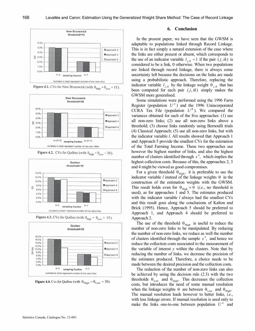
The results of the study are presented in Figures 2.1 to 2.4, Table 2, and Figure 3. Figures 2.1 to 2.4 provide bar charts of the CVs obtained for each of the five approaches. The bar charts are given for the eight cases obtained by crossing the two provinces Québec and New Brunswick, the two sampling fractions 30% and 70%, and the two thresholds 15 and 30. On each bar of the charts, one can find the number of nonzero links between A U and B U for each

of the five approaches. Note that for Approach 3, it corresponds in fact to the expected number of nonzero links. The number of (expected) nonzero links does not change from one sampling fraction to another. Table 2 shows the average number of clusters interviewed by approach, for each of the eight cases, where the average is taken over the 500 samples used for the simulations. The numbers in parenthesis are the standard deviations. They are relatively small compared to the averages and therefore the number of clusters identified through the sample A s does not fluctuate greatly from one sample A s to another. Figure 3 provides scattered plots of the obtained CVs by the average number of clusters identified through the sample , A s for each of the eight cases. By looking at the Figures 2.1 to 2.4, it can be seen that in

all cases, Approach 1 and Approach 5 provided the smallest CVs for the estimation of the Total Farming Income. Therefore, using all nonzero links yield the greatest precision. Note however that by looking at Table 2, we can see that these approaches also lead to the highest number of clusters identified through the sample selected from . A U In fact, we can see that the greater the number of clusters used in the estimation is, the greater the precision of the resulting estimates is. This result is shown in Figure 3 where we can see that the CVs tend to decrease as the average number of clusters identified through A s increases. Although this result is well known in the classical sampling theory, it was not guaranteed to hold in the context of the GWSM. As we can see from equation (3.5), it is not the sample size of A s that increases, but rather the homogeneity of the derived variables . j Z

Now, by comparing Approach 1 and Approach 5, it can be seen that the latter always provided the smallest variance. Therefore, this suggests to use the indicator variable l instead of the linkage weight θ when using all nonzero links. Note that it seems this can be generalised since the same phenomenon occurred with Approach 2 and Approach 4 (Classical Approach). Recall that, because High Low , θ = θ the two approaches differ only in the definition of the estimation weights obtained by the GWSM. Approach 2 uses the linkage weights , θ while the Classical Approach uses the indicator variables l. Note that this results goes along the conclusions of Kalton and Brick (1995) since the optimal choice of letting the constants α being 0 for some units and a positive value that is equal for all the remaining units within the cluster corresponds to the use of the indicator variable l.

We now concentrate on Approach 3. For seven out of the eight histograms of Figures 2.1 to 2.4, Approach 3 produced the highest CVs. The only lower CV was obtained for Québec, with the sampling fraction of 30% and the threshold High 30. θ = It should however be noted that this approach is the one that used the lowest number of nonzero links, and also the lowest average number of clusters identified through . A s Therefore, this result is not totally surprising. Recall that the number of nonzero links



used by Approach 3 does not depend on the threshold High θ and thus the CVs obtained for Québec with 0.3 f = were equal for High 15 θ = and High 30. θ = For High 15, θ = the CV obtained for Approach 3 for Québec was higher than the ones for Approaches 2 and 4, and these two were using more nonzero links, and more clusters. For High 30 θ = the CV obtained for Approach 3 was lower than the ones from approaches 2 and 4, but these two were still using more non zero links, and more clusters. Therefore, there are intermediate situations where with High 15 30, < θ < we should get equal CVs for approaches 3 and 2, and approaches 3 and 4. As a consequence, to get equal CVs between Approach 3 and each of approaches 2 and 4, more nonzero links and more clusters must be used by the latter. This suggests that in some cases, Approach 3 might be more appropriate to use than approaches 2 and 4 because estimates with the same precision can be obtained with lower collection costs.

In order to better compare Approach 3 to the approaches 2 and 4, we forced the number of expected nonzero links to be the same as the number of nonzero links used by approaches 2 and 4. For this, we have transformed the linkage weights , j ik θ to , j ik θ % % in order to have

, 0 1 1 1

B A i M M N

j ik j i k

L = = =

θ = ∑ ∑ ∑ % % (5.5)

where 0 L is the desired number of nonzero links. The transformation used was

, ,

, / if 1

1 otherwise

j ik j ik

j ik

θ θ θ ≤ θ = θ

i i

% % (5.6)

where θ i was determined iteratively such that (5.5) is satisfied. The use of Approach 3 with the transformation (5.6) is referred to as Approach 6. The results of the simulations are presented in Figures 4.1 to 4.4. As we can see, Approach 6 turned out to have the smallest CVs for half of the cases. For the other cases, Approach 4 yielded the best precision. Note that this situation did not occur for a particular province only, nor a particular sampling fraction, and also nor for a particular threshold. It would therefore be difficult in practice to determine in advance which of Approach 6 or Approach 4 would produce the smallest CVs. Because of this, and because of the fact that Approach 6 (and Approach 3) can produce large linkage errors, Approach 4 should be preferred.

Figure 2.2. CVs for NewBrunswick High Low (with 30). θ = θ =

Figure 2.1. CVs for NewBrunswick High Low (with 15). θ = θ =

Figure 2.3. CVs for Québec High Low (with 15). θ = θ =

Figure 2.4. CVs for Québec High Low (with 30). θ = θ =



Table 2 Average Number of Identified Cluster

Threshold Approach Average number of identified clusters (s.e.) Québec New Brunswick

f 0.3 = f 0.7 = f 0.3 = f 0.7 = 1 15,752(58) 21,106(30) 1,709(18) 2,100(7) 2 14,281(49) 20,593(34) 1,310(17) 1,966(13)

15 3 10,930(50) 18,881(47) 1,123(14) 1,869(14) 4 14,281(49) 20,593(34) 1,310(17) 1,966(13) 5 15,752(58) 21,106(30) 1,709(18) 2,100(7) 1 15,752(58) 21,106(30) 1,709(18) 2,100(7) 2 11,310(45) 19,139(37) 1,215(17) 1,924(15)

30 3 10,930(50) 18,881(47) 1,123(14) 1,869(14) 4 11,310(45) 19,139(37) 1,215(17) 1,924(15) 5 15,752(58) 21,106(30) 1,709(18) 2,100(7)

Figure 3. Graphs of CVs versus average number of identified clusters.



Figure 4.4. Cvs for Québec (with High Low 30). θ = θ =

6. Conclusion

In the present paper, we have seen that the GWSM is adaptable to populations linked through Record Linkage. This is in fact simply a natural extension of the case where the links are either present or absent, which corresponds to the use of an indicator variable , 1 j ik l = if the pair ( , ) j ik is considered to be a link, 0 otherwise. When two populations are linked through record linkage, there is always some uncertainty left because the decisions on the links are made using a probabilistic approach. Therefore, replacing the indicator variable , j ik l by the linkage weight , j ik θ that has been computed for each pair ( , ) j ik simply makes the GWSM more generalised.

Some simulations were performed using the 1996 Farm Register (population A U ) and the 1996 Unincorporated CCRA Tax File (population B U ). We compared the variances obtained for each of the five approaches: (1) use all nonzero links; (2) use all nonzero links above a threshold; (3) choose links randomly using Bernoulli trials (4) Classical Approach; (5) use all nonzero links, but with the indicator variable l. All results showed that Approach 1 and Approach 5 provide the smallest CVs for the estimation of the Total Farming Income. These two approaches use however the highest number of links, and also the highest number of clusters identified through , A s which implies the highest collection costs. Because of this, the approaches 2, 3 and 4 might be viewed as good compromises.

For a given threshold High , θ it is preferable to use the indicator variable l instead of the linkage weights θ in the construction of the estimation weights with the GWSM. This result holds even for High 0 θ = (i.e., no threshold is used), as for approaches 1 and 5. The estimates produced with the indicator variable l always had the smallest CVs and this result goes along the conclusions of Kalton and Brick (1995). Hence, Approach 5 should be preferred to Approach 1, and Approach 4 should be preferred to Approach 2.

The use of the threshold High θ is useful to reduce the number of nonzero links to be manipulated. By reducing the number of nonzero links, we reduce as well the number of clusters identified through the sample , A s and hence we reduce the collection costs associated to the measurement of the variable of interest y within the clusters. Note that by reducing the number of links, we decrease the precision of the estimates produced. Therefore, a choice needs to be made between the desired precision and the collection costs.

The reduction of the number of nonzero links can also be achieved by using the decision rule (2.3) with the two thresholds Low θ and High . θ This decreases the collection costs, but introduces the need of some manual resolution when the linkage weights θ are between Low θ and High . θ The manual resolution leads however to better links, i.e., with less linkage errors. If manual resolution is used only to make the links onetoone between population A U and



population , B U then it might not be necessary since the GWSM is particularly appropriate to handle estimation in situations where the links between A U and B U are complex.

When compared to approaches 2 and 4, Approach 3 turned out to be preferable in some cases. Because it would be difficult in practice to determine in advance which of Approach 3 or Approach 4 would produce the smallest CVs, and because of the fact that Approach 3 can produce large linkage errors, Approach 4 should be preferred. Hence, the Classical Approach of using the GWSM with the indicator variable l with links determined using a decision rule such as (2.3) seems the most appropriate approach to estimate the total B Y using a sample selected from . A U

Acknowledgements

The authors would like to thank the Associate Editor and the two referees for their useful suggestions and comments. These have contributed to improve significantly the quality of the paper.

References

Bartlett, S., Krewski, D., Wang, Y. and Zielinski, J.M. (1993). Evaluation of error rates in large scale computerized record linkage studies. Survey Methodology, 19, 312.

Belin, T.R. (1993). Evaluation of sources of variation in record linkage through a factorial experiment. Survey Methodology, 19, 1329.

Budd, E.C. (1971). The creation of a microdata file for estimating the size distribution of income. The Review of Income and Wealth, 17, 317333.

Budd, E.C., and Radner, D.B. (1969). The OBE size distributions series: methods and tentative results for 1964. American Economic Review, Papers and Proceedings, LIX, 435449.

Ernst, L. (1989). Weighting issues for longitudinal household and family estimates. In Panel Surveys, (Eds. D. Kasprzyk, G. Duncan, G. Kalton and M.P. Singh). New York: John Wiley & Sons, Inc., 135159.

Fellegi, I.P., and Sunter, A. (1969). A theory for record linkage. Journal of the American Statistical Association, 64, 11831210.

Gailly, B., and Lavallée, P. (1993). Insérer des nouveaux membres dans un panel longitudinal de ménages et d’individus : Simulations. CEPS/Instead, Document PSELL No. 54, Luxembourg.

Kalton, G., and Brick, J.M. (1995). Weighting schemes for household panel surveys. Survey Methodology, 21, 3344.

Lavallée, P. (1995). Crosssectional weighting of longitudinal surveys of individuals and households using the weight share method. Survey Methodology, 21, 2532.

Lim, A. (2000). Results of the Linkage between the 1998 Taxation Data and the 1998 Farm Register. Internal document of the Business Survey Methods Division, Statistics Canada.

Lynch, B.T., and Arends, W.L. (1977). Selection of a Surname Coding Procedure for the SRS Record Linkage System. Document of the Sample Survey Research Branch, Statistical Reporting Service, U.S. Department of Agriculture, Washington, D.C.

Newcome, H.B., Kennedy, J.M., Axford, S.J. and James, A.P. (1959). Automatic linkage of vital records. Science, 130, 954959.

Okner, B.A. (1972). Constructing a new data base from existing microdata sets: The 1966 merge file. Annals of Economic and Social Measurement, 1, 325342.

Särndal, C.E., Swensson, B. and Wretman, J. (1992). Model Assisted Survey Sampling. New York: SpringerVerlag.

Singh, A.C., Mantel, A.J., Kinack, M.D. and Rowe, G. (1993). Statistical matching: Use of auxiliary information as an alternative to the conditional independence assumption. Survey Methodology, 19, 5979.

Statistics Canada (2000). Whole Farm Database reference manual. Publication No. 21F0005GIE, Statistics Canada, 100 pages.

Thompson, S.K. (1992). Sampling. New York: John Wiley & Sons, Inc.

Thompson, S.K., and Seber, G.A. (1996). Adaptive Sampling. New York: John Wiley & Sons, Inc.

Winkler, W.E. (1995). Matching and record linkage. Business Survey Methods, (Eds. B.G. Cox, D.A. Binder, B.N. Chinnappa, A. Christianson, M.J. Colledge and P.S. Kott), New York: John Wiley & Sons, Inc., 355384.

Yates, F., and Grundy, P.M. (1953). Selection without replacement from within strata with probability proportional to size. Journal of the Royal Statistical Society, B, 15, 235261.

Estimation Using the Generalised Weight Share...

Documents

Transcript of Estimation Using the Generalised Weight Share...